0-realbookstyleandnotation
TRANSCRIPT

Riccardo Rigon
The Real Books:On Style and Notation
R. R
igon
- Il
tav
olo
di
lavo
ro d
i R
emo w
olf
Tuesday, February 26, 13

“Standards are nice if each one of us has his own”
Sandro Marani
Tuesday, February 26, 13
R. Rigon
3
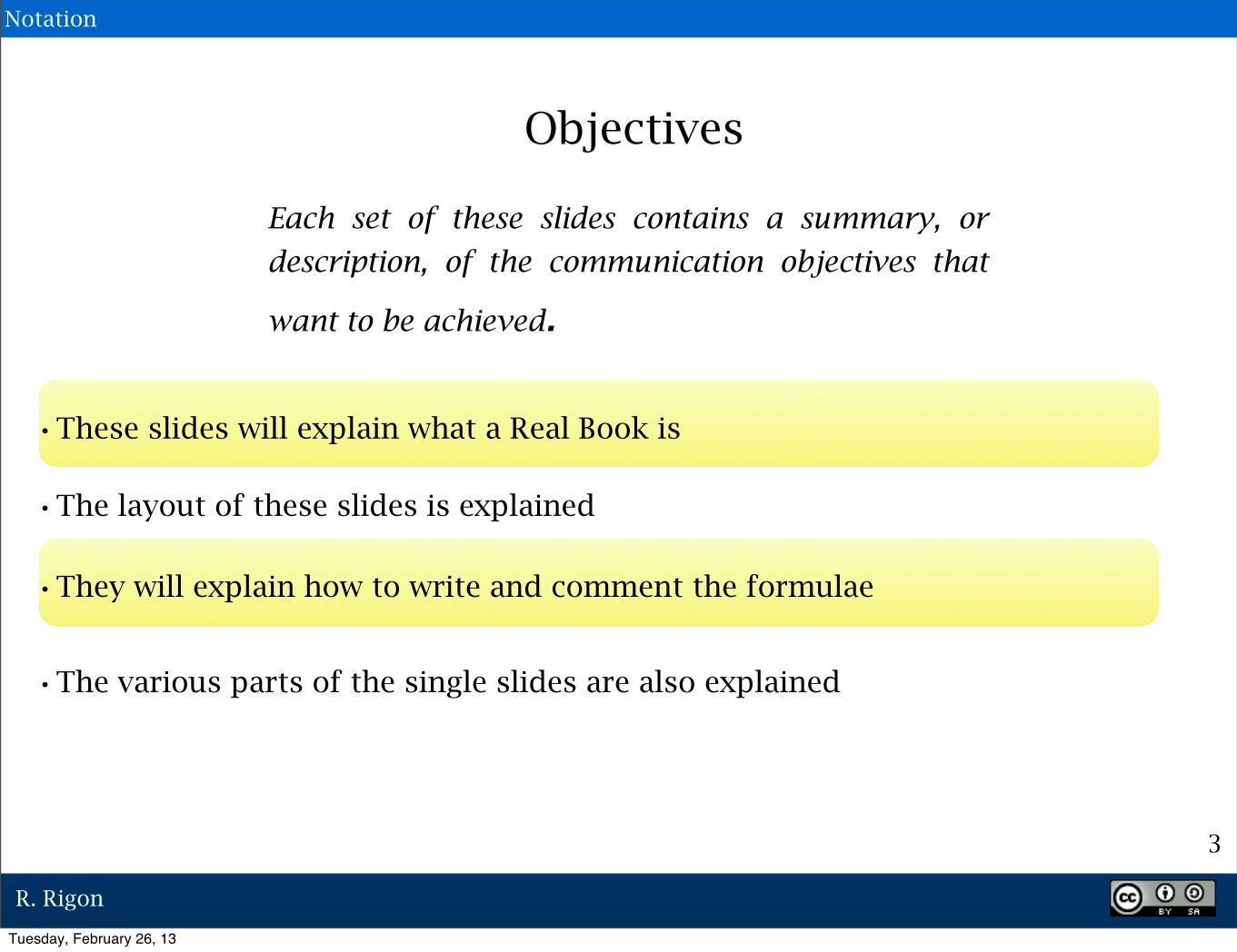
Objectives
Each set of these slides contains a summary, or
description, of the communication objectives that
want to be achieved.
•These slides will explain what a Real Book is
•The layout of these slides is explained
•They will explain how to write and comment the formulae
•The various parts of the single slides are also explained
Notation
Tuesday, February 26, 13

R. Rigon
4
Notes on Style
For these slides I have chosen to use the Lucida Bright font, at 24 point size,
with justified text. The titles have been centred and they have been written in a
36 point Lucida Bright font.
The notes are in 18 point Lucida Bright. The references are in 14 point Lucida
Bright.
The choice of font is linked to the formulae, which are pdf images created
with LaTeX (specifically LaTeXit! for Mac), using the Computer Modern font,
which is very similar to Lucida Bright. The formulae usually use a 36 point font
size. There follows an example.
dM�dt
= P � �H�f
�f
Notation
Tuesday, February 26, 13

R. Rigon
5
dM�dt
= P � �H�f
�f
Conservation of mass of snow
Notes on Style
Experience teaches that, in order to reproduce the communicative effect of
writing by hand on a blackboard, the formulae need to commented. For these
slides I have chosen the following method: the formula is “boxed” in red (2 pt)
and a red arrow points to an explanation in italics.
Notation
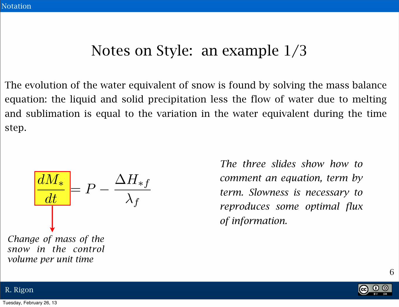
The three slides show how to
comment an equation, term by
term. Slowness is necessary to
reproduces some optimal flux
of information.
Tuesday, February 26, 13
R. Rigon
6
Notes on Style: an example 1/3
The evolution of the water equivalent of snow is found by solving the mass balance
equation: the liquid and solid precipitation less the flow of water due to melting
and sublimation is equal to the variation in the water equivalent during the time
step.
dM�dt
= P � �H�f
�f
Change of mass of the snow in the control volume per unit time
Notation
The three slides show how to
comment an equation, term by
term. Slowness is necessary to
reproduces some optimal flux
of information.
Tuesday, February 26, 13
R. Rigon
7
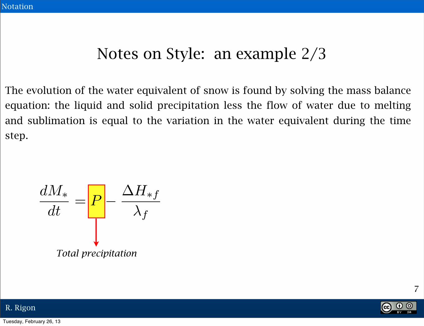
The evolution of the water equivalent of snow is found by solving the mass balance
equation: the liquid and solid precipitation less the flow of water due to melting
and sublimation is equal to the variation in the water equivalent during the time
step.
dM�dt
= P � �H�f
�f
Total precipitation
Notes on Style: an example 2/3
Notation
Tuesday, February 26, 13
R. Rigon
8
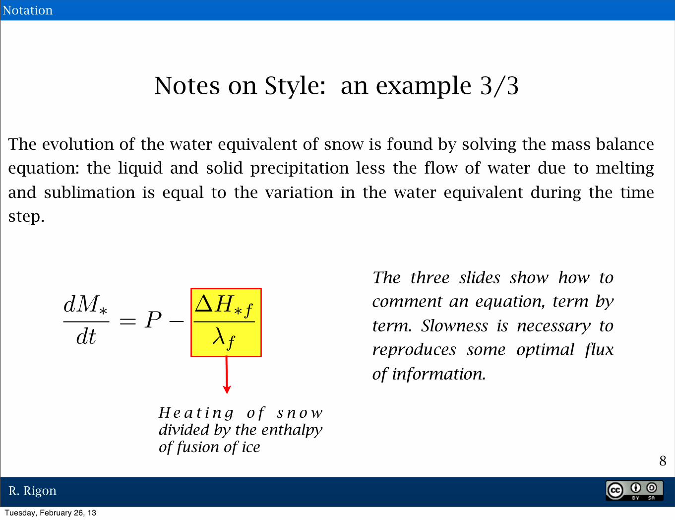
The evolution of the water equivalent of snow is found by solving the mass balance
equation: the liquid and solid precipitation less the flow of water due to melting
and sublimation is equal to the variation in the water equivalent during the time
step.
dM�dt
= P � �H�f
�f
H e a t i n g o f s n o w divided by the enthalpy of fusion of ice
Notes on Style: an example 3/3
Notation
The three slides show how to
comment an equation, term by
term. Slowness is necessary to
reproduces some optimal flux
of information.
Tuesday, February 26, 13

R. Rigon
9
The slides have some standard information: a general index
The slides have some standard information: the authors of the contribution
The slide number: gives the audience a reference point
For these slides a Creative Commons License has been used (http.cc)
Notes on Style:
The centre of the
slide is white: this is
f o r i m p r o v e d
visibility and to avoid
w a s t a g e o f t o n e r
when printing. The
cover slide, on the
other hand, is all blue
with an image.
The slides have some standard information: authors
NotationR
igon
, 20
13
Tuesday, February 26, 13

R. Rigon
10
Other Notes:
The formulae have been written using LaTeXit, and they are alive, in the
sense that dragging them back to LaTeXit, the code that generated them
reappears.
Generally, wherever possible, parts of the calculation code or graphic
generation code are also given.
Notation
Tuesday, February 26, 13
R. Rigon
11
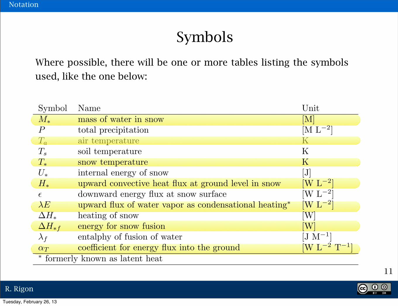
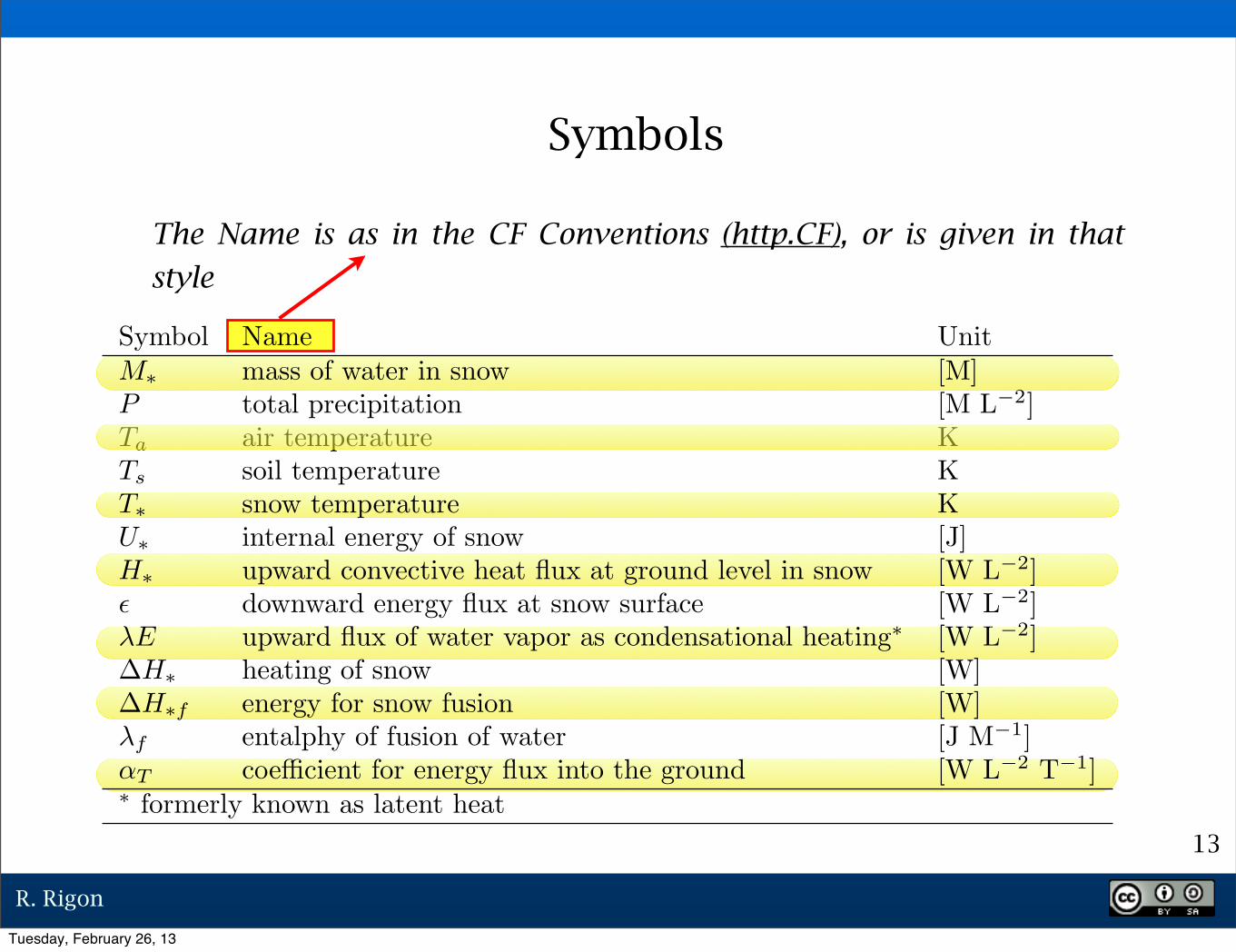
Symbols
Where possible, there will be one or more tables listing the symbols
used, like the one below:
Notation
Tuesday, February 26, 13

R. Rigon
12
Symbols
The aim, wherever possible, is to use standard symbols that are
different for different quantities.
Tuesday, February 26, 13
R. Rigon
13
Symbols
The Name is as in the CF Conventions (http.CF), or is given in that
style
Tuesday, February 26, 13

R. Rigon
14
SymbolsThe unit of measure
should always be shown
Tuesday, February 26, 13

R. Rigon
15
Risorse web
•http.wp - http://en.wikipedia.org/wiki/Real_Book - Last accessed May, 7, 2009
•http.cc - http://creative.commons.org - Last accessed May, 7, 2009
•http.CF -http://cf-pcmdi.llnl.gov/
Tuesday, February 26, 13
R. Rigon
16
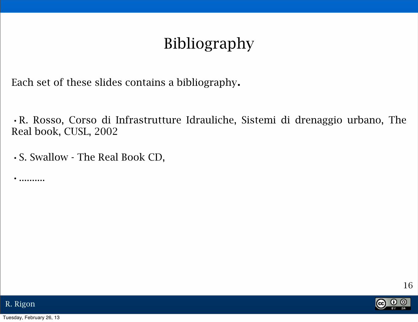
Bibliography
Each set of these slides contains a bibliography.
•S. Swallow - The Real Book CD,
•R. Rosso, Corso di Infrastrutture Idrauliche, Sistemi di drenaggio urbano, The Real book, CUSL, 2002
•..........
Tuesday, February 26, 13

Basic Notation for Scalar, Vector and Tensor Fields, and Matrices
Bru
no M
un
ari
- Li
bri
ill
eggib
ili
Tuesday, February 26, 13

R. Rigon
18
Objectives
•In these slides the notational rules used in the Real Books are defined.
•In particular, explanation is given on how to write the formulae so that the
indices and various graphic aspects can be interpreted univocally.
•However these are guidelines that can be violated in practical cases in favor
of simplicity of notation.
Tuesday, February 26, 13

R. Rigon
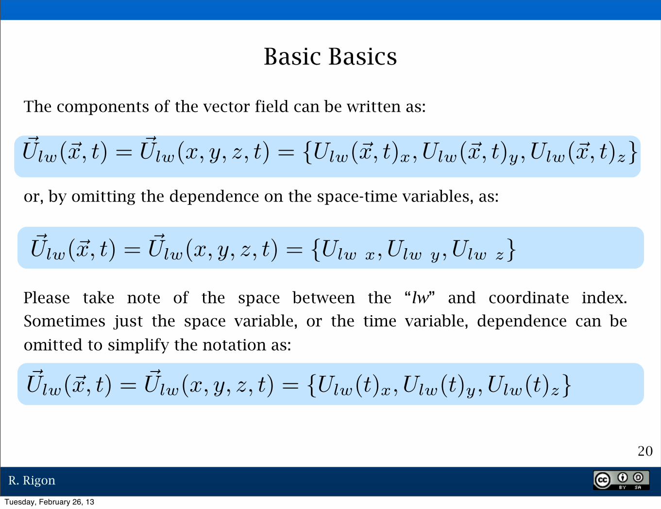
Let Ulw be a space-time field. Then
Ulw(⌥x, t) = Ulw(x, y, z, t)
is a scalar field. The field can be independent of some space variable or
time, which is then omitted. Whether the vector is 2-D or 3-D depends
on the context. On the other hand
is a vector field. Other notations for vectors are possible, but not used.
⌥Ulw(⌥x, t) = ⌥Ulw(x, y, z, t)
⌥Ulw(⌥x, t) = ⌥Ulw(x, y, z, t) = {Ulw(⌥x, t)x, Ulw(⌥x, t)y, Ulw(⌥x, t)z}
Basic Basics
19
Tuesday, February 26, 13
R. Rigon
⌥Ulw(⌥x, t) = ⌥Ulw(x, y, z, t) = {Ulw(⌥x, t)x, Ulw(⌥x, t)y, Ulw(⌥x, t)z}
The components of the vector field can be written as:
or, by omitting the dependence on the space-time variables, as:
⌥Ulw(⌥x, t) = ⌥Ulw(x, y, z, t) = {Ulw x, Ulw y, Ulw z}
Please take note of the space between the “lw” and coordinate index.
Sometimes just the space variable, or the time variable, dependence can be
omitted to simplify the notation as:
⌥Ulw(⌥x, t) = ⌥Ulw(x, y, z, t) = {Ulw(t)x, Ulw(t)y, Ulw(t)z}
Basic Basics
20
Tuesday, February 26, 13
R. Rigon
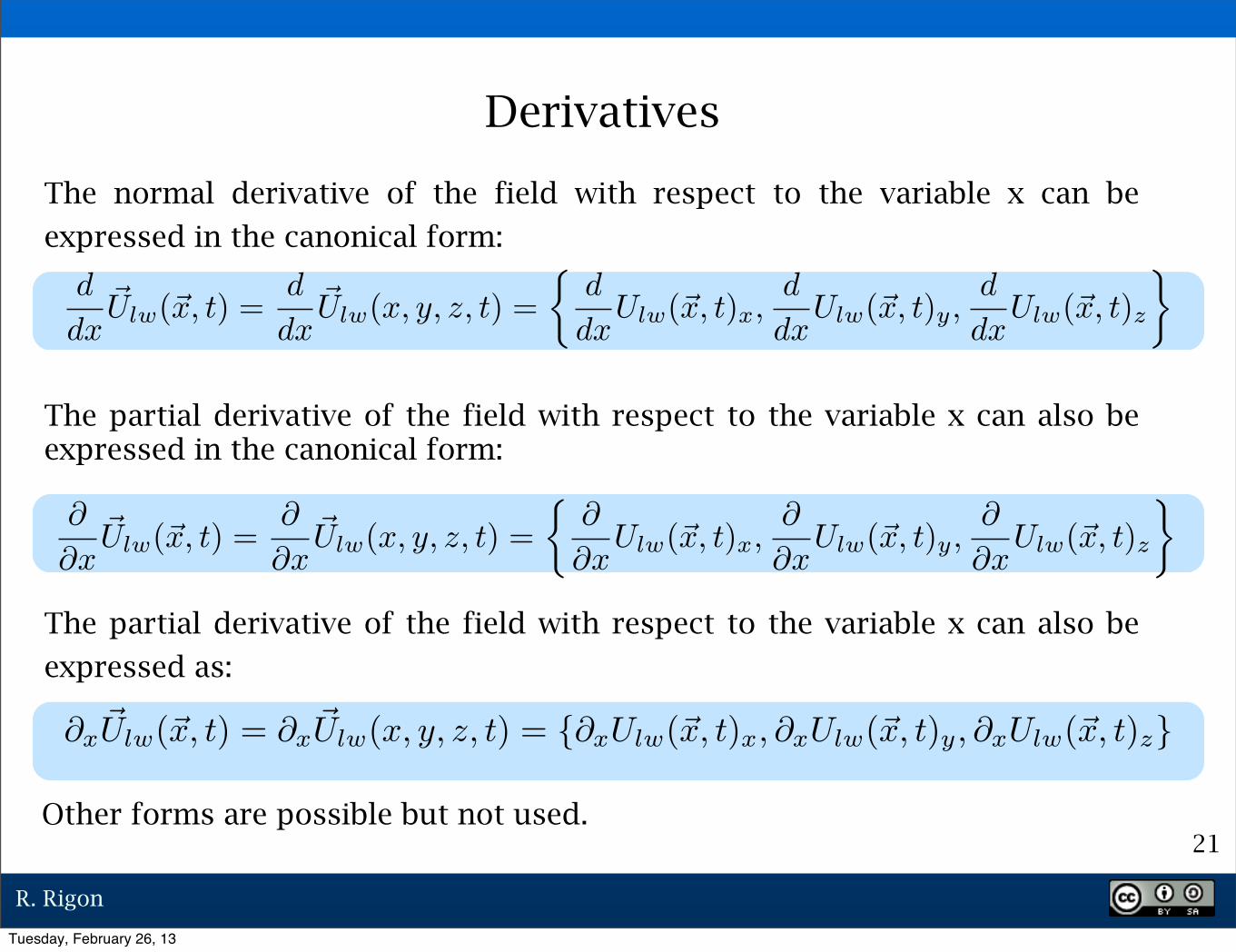
The normal derivative of the field with respect to the variable x can be
expressed in the canonical form:
d
dx�Ulw(�x, t) =
d
dx�Ulw(x, y, z, t) =
�d
dxUlw(�x, t)x,
d
dxUlw(�x, t)y,
d
dxUlw(�x, t)z
⇥
⇥x�Ulw(�x, t) = ⇥x
�Ulw(x, y, z, t) = {⇥xUlw(�x, t)x, ⇥xUlw(�x, t)y, ⇥xUlw(�x, t)z}
The partial derivative of the field with respect to the variable x can also be
expressed as:
The partial derivative of the field with respect to the variable x can also be expressed in the canonical form:
Other forms are possible but not used.
⇥
⇥x�Ulw(�x, t) =
⇥
⇥x�Ulw(x, y, z, t) =
�⇥
⇥xUlw(�x, t)x,
⇥
⇥xUlw(�x, t)y,
⇥
⇥xUlw(�x, t)z
⇥
Derivatives
21
Tuesday, February 26, 13
R. Rigon
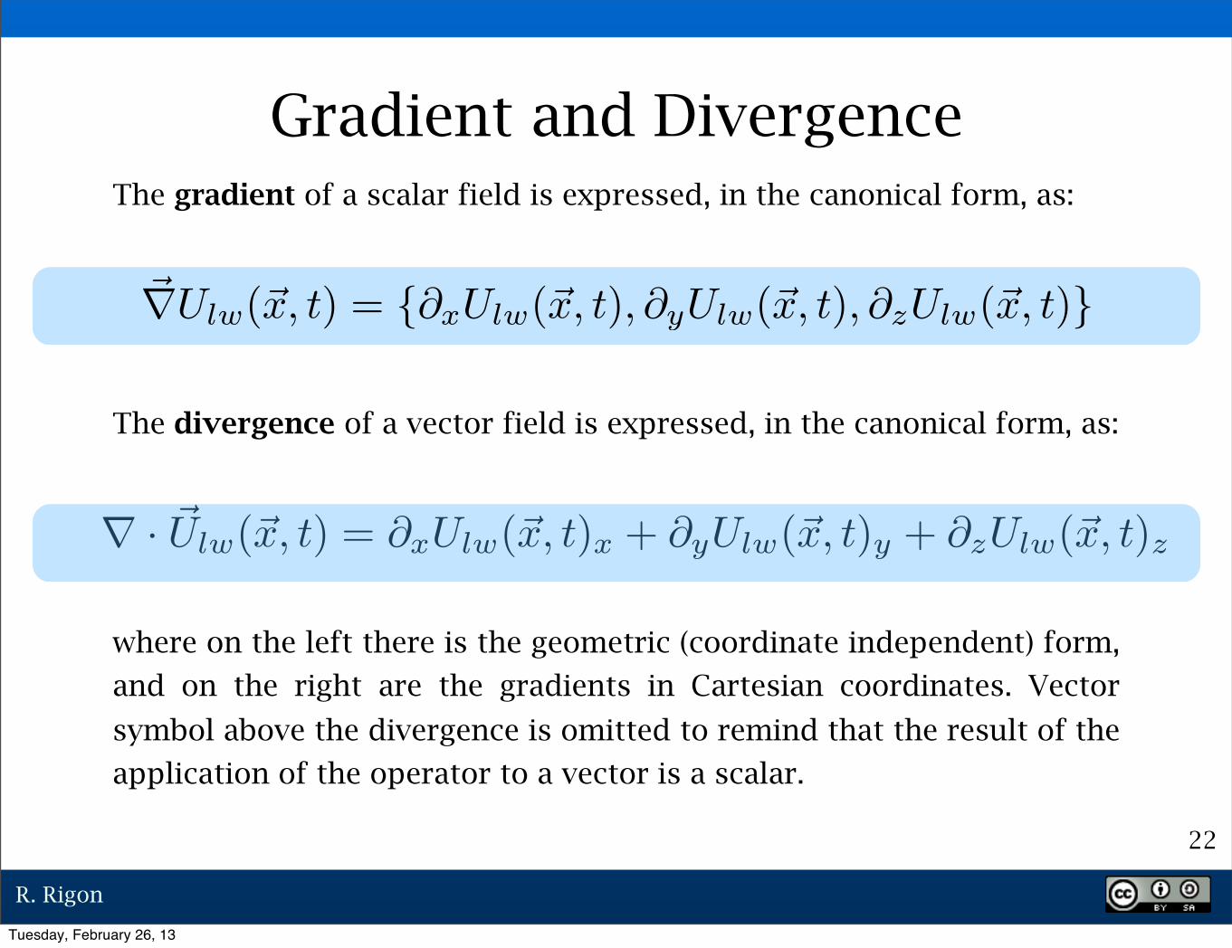
Gradient and DivergenceThe gradient of a scalar field is expressed, in the canonical form, as:
⌃⇤Ulw(⌃x, t) = {⇥xUlw(⌃x, t), ⇥yUlw(⌃x, t), ⇥zUlw(⌃x, t)}
The divergence of a vector field is expressed, in the canonical form, as:
where on the left there is the geometric (coordinate independent) form,
and on the right are the gradients in Cartesian coordinates. Vector
symbol above the divergence is omitted to remind that the result of the
application of the operator to a vector is a scalar.
⇥ · ⌃Ulw(⌃x, t) = ⇥xUlw(⌃x, t)x + ⇥yUlw(⌃x, t)y + ⇥zUlw(⌃x, t)z
22
Tuesday, February 26, 13

R. Rigon
Gradient and Divergence
The divergence can also be expressed in a more compact form using
the Einstein summation convention:
meaning that when an index variable appears twice in a single term,
once in an upper (superscript) and once in a lower (subscript) position,
there is a summation over all of its possible values.
i � {x, y, x}
⇥ · ⌃Ulw(⌃x, t) = ⇥iUlw(⌃x, t)i = ⇥iUlw(⌃x, t)i
23
Tuesday, February 26, 13
R. Rigon
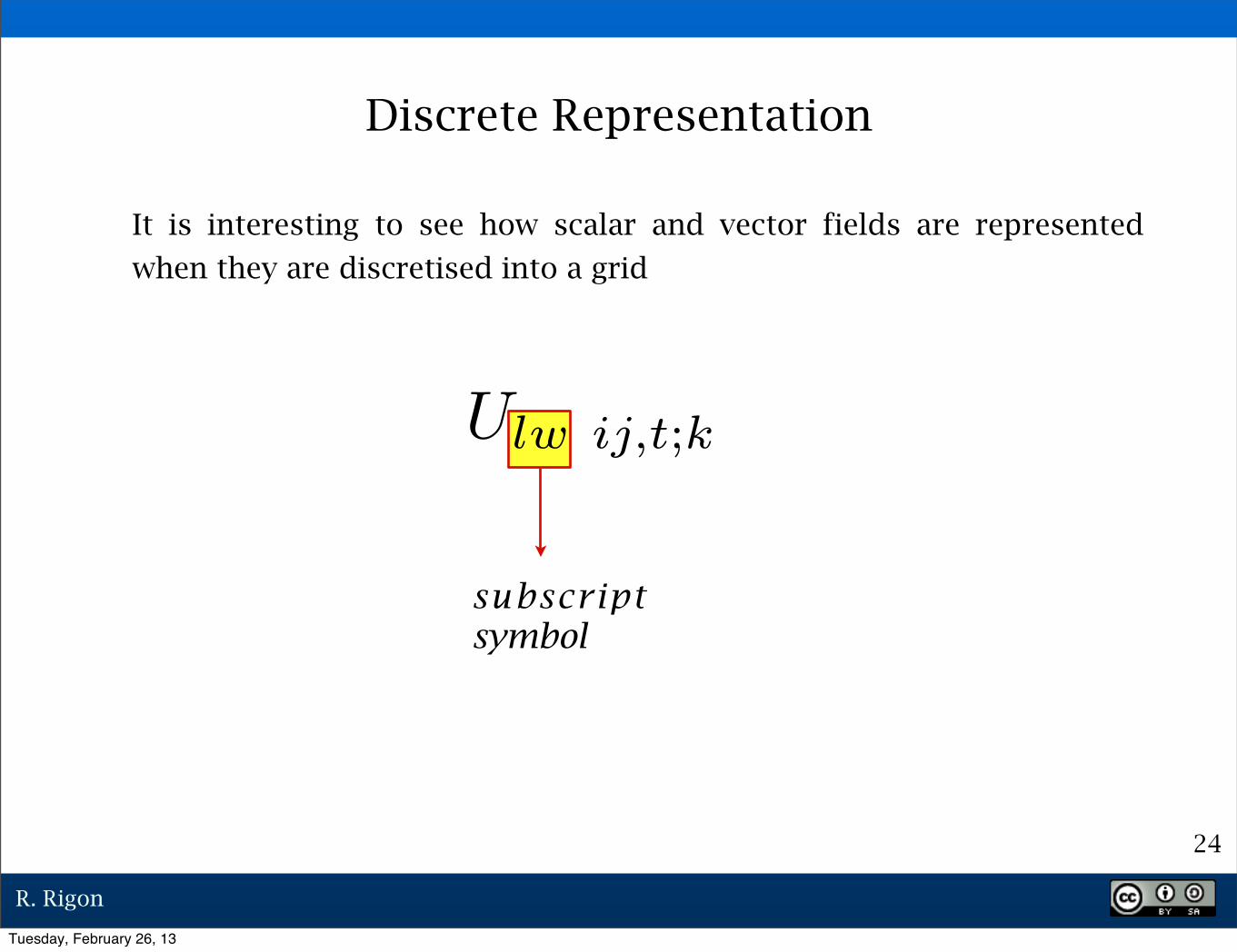
Discrete Representation
It is interesting to see how scalar and vector fields are represented
when they are discretised into a grid
Ulw ij,t;k
subscript symbol
24
Tuesday, February 26, 13

R. Rigon
It is interesting to see how scalar and vector fields are represented
when they are discretised into a grid
Ulw ij,t;k
e m p t y space
Discrete Representation
25
Tuesday, February 26, 13

R. Rigon
It is interesting to see how scalar and vector fields are represented
when they are discretised into a grid
Ulw ij,t;k
spatial index, first index refers to the cell (center) the second to the cell face, which is then j(i). If only one index is present it is a cell index.
26
Discrete Representation
Tuesday, February 26, 13

R. Rigon
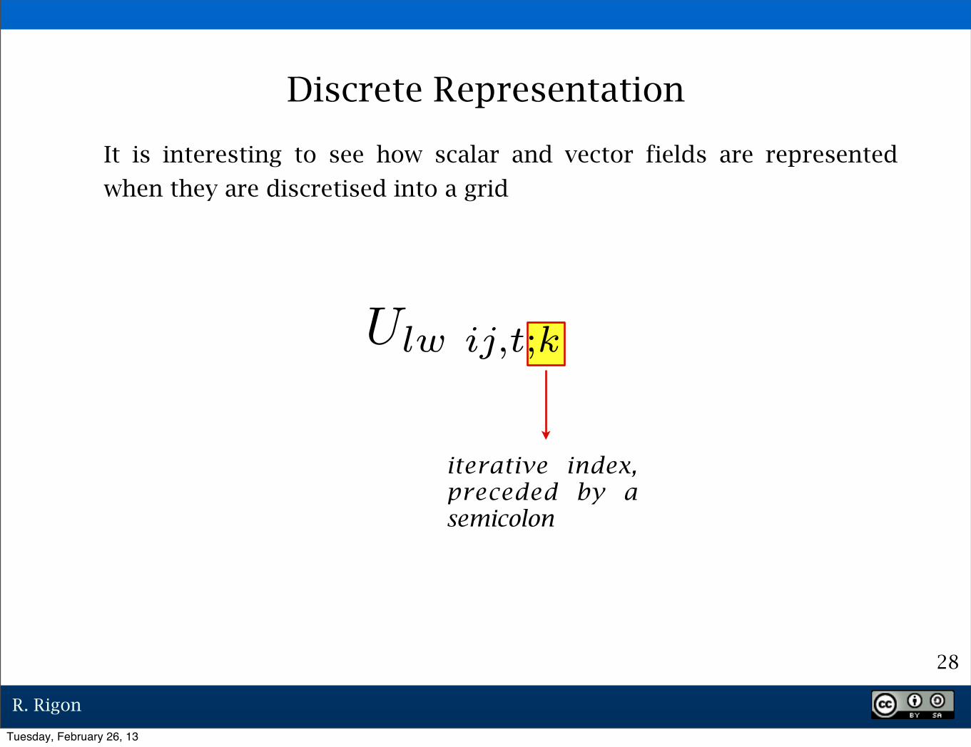
It is interesting to see how scalar and vector fields are represented
when they are discretised into a grid
Ulw ij,t;k
t e m p o r a l i n d e x , preceded by a comma
27
Discrete Representation
Tuesday, February 26, 13
R. Rigon
It is interesting to see how scalar and vector fields are represented
when they are discretised into a grid
Ulw ij,t;k
iterative index, preceded by a semicolon
Discrete Representation
28
Tuesday, February 26, 13
R. Rigon
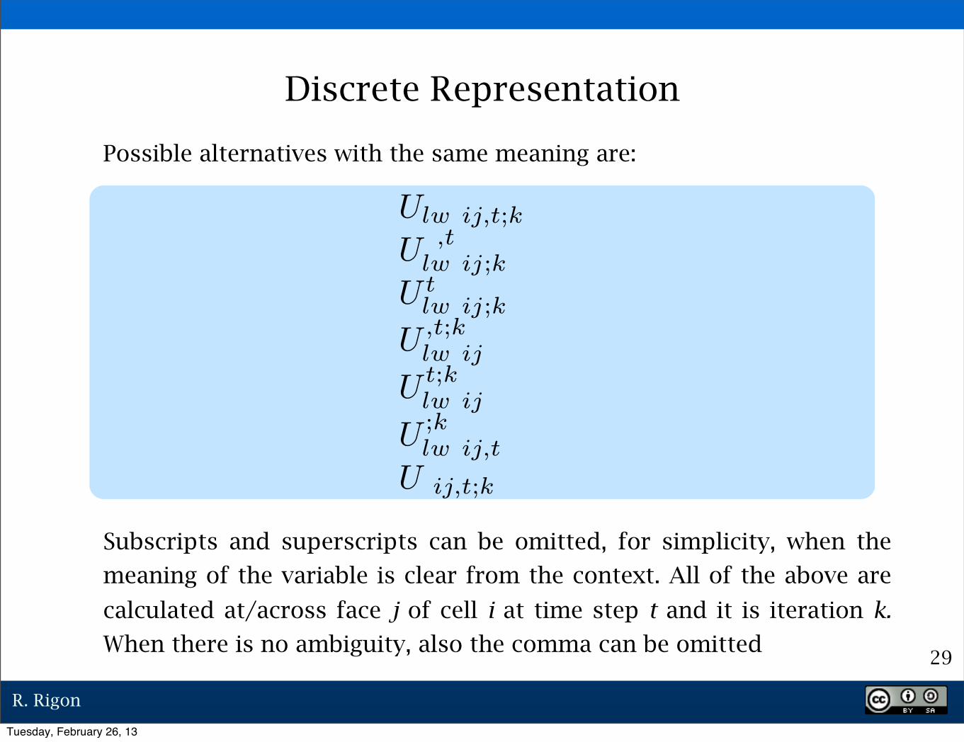
Possible alternatives with the same meaning are:
Subscripts and superscripts can be omitted, for simplicity, when the
meaning of the variable is clear from the context. All of the above are
calculated at/across face j of cell i at time step t and it is iteration k.
When there is no ambiguity, also the comma can be omitted29
Discrete Representation
Tuesday, February 26, 13

R. Rigon
Possible alternatives with the same meaning are:
30
Discrete Representation
All the above quantities are calculated for cell i at time step t and it is
iteration k
Tuesday, February 26, 13

R. Rigon
31
Discrete Representation
When a single index is presented, it can be, for instance
with varying i. Therefore, a “vector”, meaning an array of data, can be built:
Tuesday, February 26, 13

R. Rigon
32
Discrete Representation
where the symbol is used to identify a column vector
Tuesday, February 26, 13

R. Rigon
33
Discrete Representation
where the symbol is used to identify a row type of vector
Tuesday, February 26, 13

R. Rigon
34
Discrete Representation
The two symbols
or “harpoon” are used for distinguishing this type of vector from the spatial euclidean vectors that have certain particular transformation rules upon rotations in space.
Tuesday, February 26, 13
R. Rigon
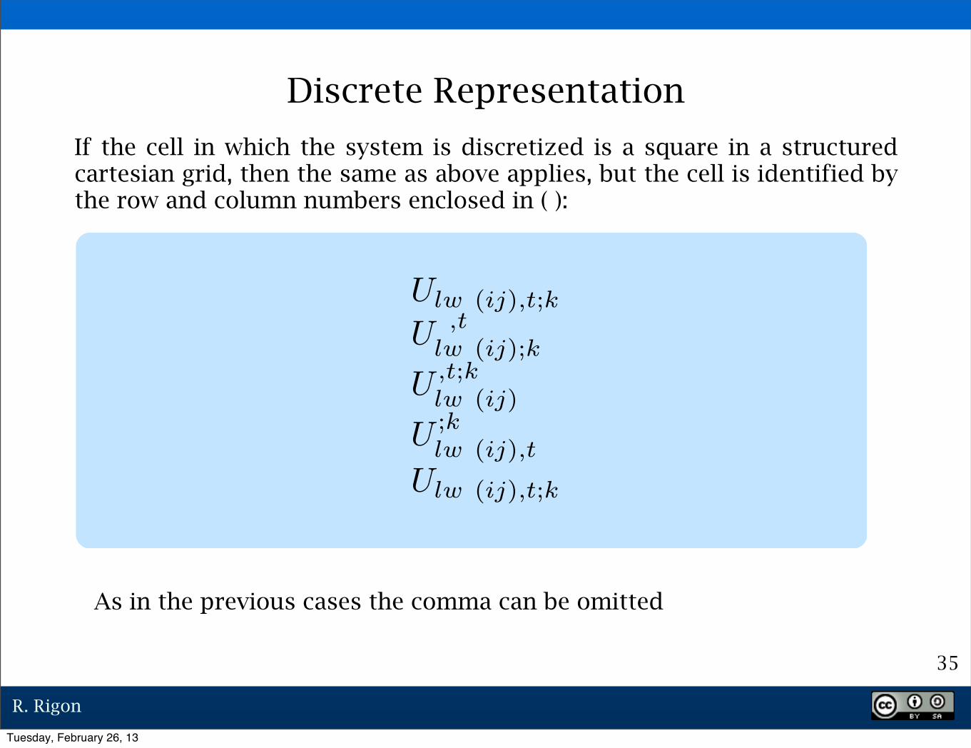
If the cell in which the system is discretized is a square in a structured cartesian grid, then the same as above applies, but the cell is identified by the row and column numbers enclosed in ( ):
Discrete Representation
35
As in the previous cases the comma can be omitted
Tuesday, February 26, 13

R. Rigon
If the cell is a square in a structured cartesian grid, then the same as above applies, but the cell face is identified by the row and column numbers enclosed in ( ) with +1/2 (or -1/2)
36
Discrete Representation
Tuesday, February 26, 13

R. Rigon
Cell points and face points in a structured grid:
37
Discrete Representation
Tuesday, February 26, 13

R. Rigon
If position or time or iteration are identifiable from the context, or they are unimportant or a non-applicable feature, then they can be omitted
means the field Ulw at the face between position i,j and i,j+1 in a cartesian grid at a known time.
Ulw i
means the field Ulw at cell i in an unstructured grid at a known or unspecified time.
U ,tlw
means the field Ulw at a generic cell at time t
Discrete Representation
38
Tuesday, February 26, 13

R. Rigon
⇤Ulw ij,t;k = {Ulw.x ij,t;k, Ulw.y ij,t;k, Ulw.z ij,t;k}
Discrete Representation of Vector Components
These are represented with a straightforward extension of what was used with scalars:
39
Tuesday, February 26, 13

R. Rigon
A tensors field is represented by bold letters (either lower or upper case)
Tensors
Ulw(⌃x, t) = Ulw(x, y, z, t)
In this case Ulw is a 3 x 3 tensor field with components:
�
⇤Ulw(⇧x, t)xx Ulw(⇧x, t)xy Ulw(⇧x, t)xz
Ulw(⇧x, t)yx Ulw(⇧x, t)yy Ulw(⇧x, t)yz
Ulw(⇧x, t)zx Ulw(⇧x, t)zy Ulw(⇧x, t)zz
⇥
⌅
The components are not written with bold characters.
40
Tuesday, February 26, 13

R. Rigon
41
Tensors
However, a tensor by components representation is preferable. So U becomes:
Or, when the notation is not ambiguous (not to be confounded with the (ij) element of a grid) simply:
The context says if the subscripts refer to a grid point or to the component of a tensors. This is deemed necessary to avoid extra
Tuesday, February 26, 13

R. Rigon
All the rules given for scalars and vectors apply consistently to tensors
Tensors
However, bear in mind that scalars, vectors, and tensors are geometric objects which have properties that are independent of the choice of reference system (i.e. independent of the origin, the base, and the orientation of the space-time vector space) and the coordinate system (i.e. cartesian, cylindrical or curvilinear or other).
Tensors are matrices, and matrix notation applies to tensors
42
Tuesday, February 26, 13

R. Rigon
Thus, while tensor indices always refers to space-time, matrix indices do not.
Tensors are matrices, and matrix notation applies to tensors
Remember also that divergence, gradient and curl are themselves geometric objects and obey the same rules as tensors. By changing coordinate system, they change their components but not their geometric properties.
These geometric properties, in fact, should be preserved in a proper discretisation, since they are intimately related to the Conservation Laws of Physics.
43
Tuesday, February 26, 13
R. Rigon
44
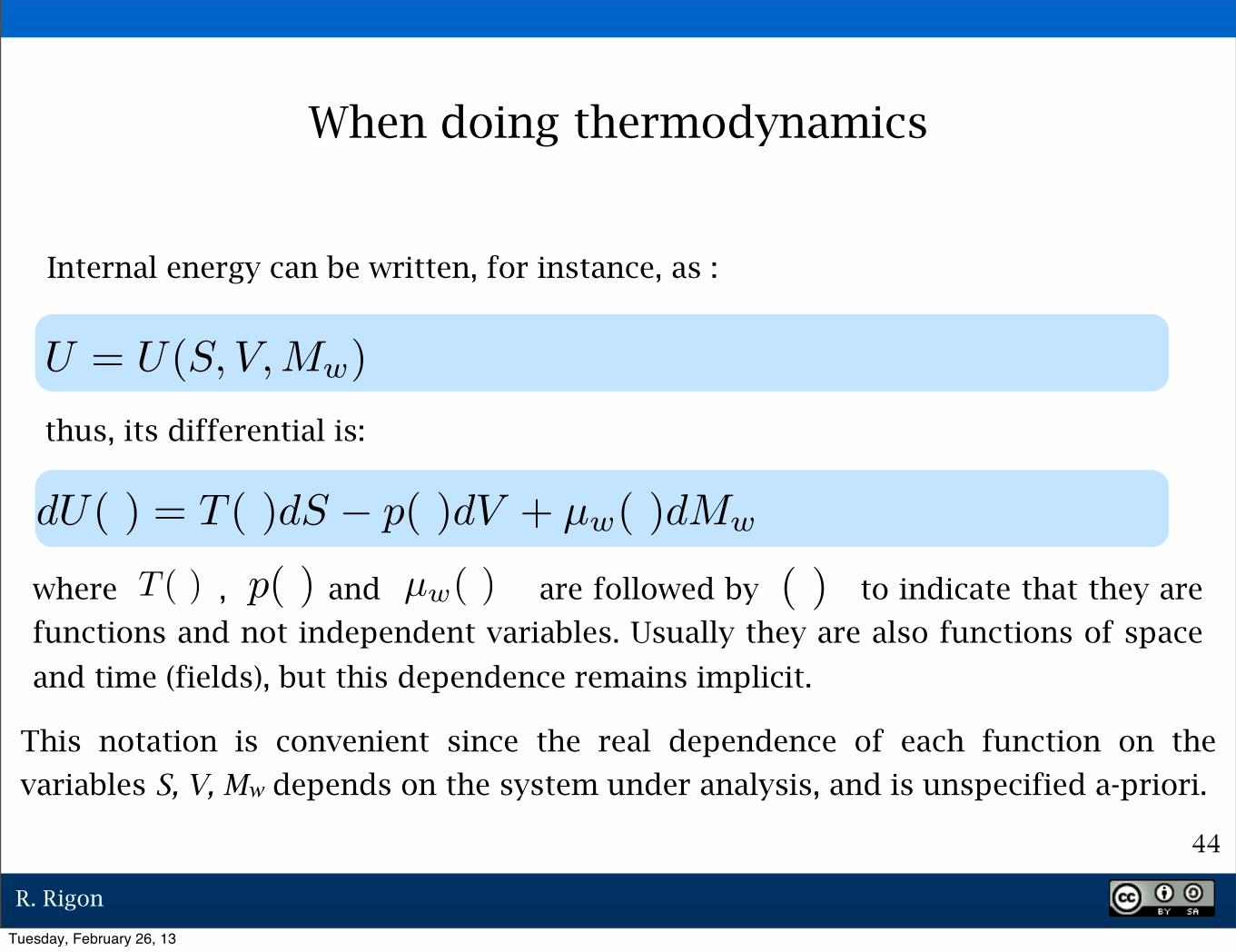
When doing thermodynamics
U = U(S, V, Mw)
thus, its differential is:
Internal energy can be written, for instance, as :
dU( ) = T ( )dS � p( )dV + µw( )dMw
where , and are followed by to indicate that they are
functions and not independent variables. Usually they are also functions of space
and time (fields), but this dependence remains implicit.
µw( )T ( ) p( ) ( )
This notation is convenient since the real dependence of each function on the
variables S, V, Mw depends on the system under analysis, and is unspecified a-priori.
Tuesday, February 26, 13
R. Rigon
Thank you for your attention.
G.U
lric
i, 2
00
0 ?
45
Tuesday, February 26, 13