0 implementing high-performance complex matrix ... · implementing high-performance complex matrix...
TRANSCRIPT

0
Implementing high-performance complex matrix multiplication via the3m and 4m methods
FIELD G. VAN ZEE and TYLER M. SMITH, The University of Texas at Austin
In this article, we explore the implementation of complex matrix multiplication. We begin by briefly identi-fying various challenges associated with the conventional approach, which calls for a carefully-written kernel
that implements complex arithmetic at the lowest possible level (i.e., assembly language). We then set out to
develop a method of complex matrix multiplication that avoids the need for complex kernels altogether. Thisconstraint promotes code reuse and portability within libraries such as BLAS and BLIS and allows kernel
developers to focus their efforts on fewer and simpler kernels. We develop two alternative approaches—onebased on the 3M method and one that reflects the classic 4M formulation—each with multiple variants,
all of which rely only upon real matrix multiplication kernels. We discuss the performance characteristics
of these so-called “induced” methods, and observe that the assembly-level method actually resides alongthe 4M spectrum of algorithmic variants. Implementations are developed within the BLIS framework, and
testing on modern hardware confirms that while the less numerically stable 3M method yields the fastest
runtimes, the more stable (and thus widely applicable) 4M method’s performance is somewhat limited dueto implementation challenges which appear inherent in nature.
CCS Concepts: rMathematics of computing→Mathematical software performance; Computationson matrices;
General Terms: Algorithms, Performance
Additional Key Words and Phrases: linear algebra, DLA, high-performance, complex, matrix, multiplication,micro-kernel, kernel, BLAS, BLIS, 3m, 4m, induced
ACM Reference Format:Field G. Van Zee and Tyler M. Smith. 2016. Implementing high-performance complex matrix multiplicationvia the 3m and 4m methods ACM Trans. Math. Softw. 0, 0, Article 0 ( 2016), 36 pages.DOI: http://dx.doi.org/10.1145/2755561
1. INTRODUCTIONHigh performance matrix multiplication resides near the bottom of the food chain forscientific and numerical applications. Implementations for matrix multiplication arecommonly accessed via the level-3 Basic Linear Algebra Subprograms (BLAS) [Don-garra et al. 1990], a subset of a standardized library API that provides routines forcomputing various types of matrix products, including general matrix-matrix multi-ply (GEMM). Many well-known projects either implement the BLAS directly [Dongarraet al. 1990; Xianyi et al. 2012; Whaley and Dongarra 1998; Van Zee and van de Geijn
This research was partially sponsored by grants from the National Science Foundation (Awards CCF-1320112, ACI-1148125/1340293, and ACI-1550493). Any opinions, findings and conclusions or recommen-dations expressed in this material are those of the author(s) and do not necessarily reflect the views of theNational Science Foundation (NSF).Authors’ addresses: Field G. Van Zee, Department of Computer Sciences and Institute for ComputationalEngineering and Sciences, The University of Texas at Austin, Austin, TX 78712, [email protected] Smith, Department of Computer Sciences, The University of Texas at Austin, Austin, TX 78712,[email protected] to make digital or hard copies of all or part of this work for personal or classroom use is grantedwithout fee provided that copies are not made or distributed for profit or commercial advantage and thatcopies bear this notice and the full citation on the first page. Copyrights for components of this work ownedby others than the author(s) must be honored. Abstracting with credit is permitted. To copy otherwise, orrepublish, to post on servers or to redistribute to lists, requires prior specific permission and/or a fee. Requestpermissions from [email protected]© 2016 Copyright held by the owner/author(s). Publication rights licensed to ACM. 0098-3500/2016/-ART0
$15.00DOI: http://dx.doi.org/10.1145/2755561
ACM Transactions on Mathematical Software, Vol. 0, No. 0, Article 0, Publication date: 2016.

0:2 F. Van Zee and T. Smith
2015; AMD 2012; IBM 2012; Intel 2014]), or build upon the matrix multiplication fa-cilities within the BLAS to perform more sophisticated dense linear algebra (DLA)computations [Van Zee et al. 2009; Anderson et al. 1999; Agullo et al. 2009; Agulloet al. 2010; Poulson et al. 2013; Choi et al. 1992]. Most BLAS operations are specifiedfor both the real and complex domains. And while multiplication of real matrices isemployed by countless applications, the unique properties of complex numbers, suchas their ability to encode both the phase and magnitude of a wave, makes complexdomain computations vitally important to many sub-fields of science and engineering,including signal processing, quantum mechanics, and control theory.
Previous work has shown that one particular algorithm for performing matrix mul-tiplication is ideal for most problem shapes [Goto and van de Geijn 2008a; 2008b; VanZee et al. 2016; Smith et al. 2014], particularly the rank-k update that frequently ap-pears within matrix factorizations (e.g. Cholesky, LU, and QR), inversions (e.g. trian-gular and Hermitian-positive definite), and transformations (e.g. block Householder).Previously expressed as three loops around a monolithic kernel [Goto and van de Geijn2008a], the state-of-the-art formulation of this algorithm consists of five loops1 arounda much smaller micro-kernel [Van Zee and van de Geijn 2015; Van Zee et al. 2016;Smith et al. 2014]. Still, these “micro-kernels” must be implemented very carefully,typically by experts who understand various characteristics of the compute hardware(such as the instruction set, instruction latencies, and the various features of the mem-ory hierarchy). Most of these kernels are implemented in low-level languages suchas machine-specific assembly language2, which unfortunately obscure the mathemat-ics being expressed. To make matters worse, very few modern architectures providemachine instructions that directly implement complex multiplication and addition,forcing kernel developers to orchestrate computation on the real and imaginary com-ponents manually.3 This can be a tedious undertaking, even for those well-versed inassembly language. While still requiring skill and knowledge of the hardware, imple-menting real domain matrix multiplication is a significantly more accessible task.
Much of the scientific computing community’s attention remains fixed on matrixmultiplication in the real domain (usually double precision). Evidence of this canbe seen most prominently in the way the community benchmarks its supercomput-ers [Dongarra et al. 1979; Dongarra et al. 2003; Top500 2015]. These codes consistlargely of an LU factorization with partial pivoting on a double-precision real densematrix. Most of the floating-point operations in an LU factorization are performed,at some level of recursion, within GEMM subproblems. Consequently, when other as-pects of the LU factorization are implemented properly, the performance of the overallbenchmark is largely determined by the performance of the double-precision GEMM(dgemm) implementation. Thus, it is no wonder that we prioritize optimizing real ma-trix multiplication kernels.
1.1. MotivationsWe have set the stage for our present work by observing that, relative to complexmatrix kernels, real matrix kernels are not only objectively easier to implement on
1This newer approach exposes two additional loops which previously, in the original algorithm, were hiddenwithin the monolithic kernel.2Low-level APIs known as vector intrinsics are sometimes used instead, typically because they fit morenaturally within higher-level languages such as C.3A notable exception to this is the IBM Blue Gene/Q architecture, which provides instructions specificallytargeting complex numbers.
ACM Transactions on Mathematical Software, Vol. 0, No. 0, Article 0, Publication date: 2016.

Implementing high-performance complex matrix multiplication via the 3m and 4m methods 0:3
many current architectures, but they are also more ubiquitous4 and quite likely to behighly optimized.
In this article, our goal is to provide a blueprint for simplifying the implementationof complex matrix multiplication, and to do so in such a way that exploits the foun-dational presence of real matrix multiplication in scientific computing environments.Specifically, we set out to investigate whether, and to what degree, real matrix kernelscan be repurposed towards the implementation of complex matrix multiplication. Thisis motivated primarily by three concerns:
— Productivity. Perhaps most obvious is the desire to minimize the number and com-plexity of kernels that must be optimized in order to support high performance withinmatrix multiplication operations. If complex kernels were, in fact, not necessarywhen computing complex matrix multiplication, then DLA library developers couldfocus on a smaller and simpler set of real domain kernels. This reduced set of kernelswould be more easily maintained on existing hardware, and allow developers to morerapidly instantiate BLAS-like functionality on new hardware.
— Portability. At its face, complex matrix multiplication is fundamentally differentfrom real matrix multiplication. (This is primarily because scalar multiplication dif-fers fundamentally in the complex domain.) Thus, if we can avoid reliance upon com-plex matrix kernels, it is not because we have avoided the mechanics of the complexdomain entirely, but rather because we have encoded the notion of complex matrixproduct at a different (higher) level. Expressing complex matrix multiplication at alevel higher than the lowest-level matrix kernel would allow us to encode the ap-proach portably within a library such as the BLAS-Like Library Instantiation Soft-ware (BLIS) framework [Van Zee and van de Geijn 2015; Van Zee et al. 2016]. If suc-cessful, this would allow developers and other experts to effectively induce complexmatrix multiplication “for free” as long as the corresponding real matrix multiplica-tion kernel is present.
— Performance. A hypothetical complex matrix multiplication based on a real domainkernel would likely inherit the performance properties of that kernel; that is, optimiz-ing the real kernel would accelerate both real and complex domain matrix multipli-cation. However, the conventional wisdom among DLA experts suggests that complexmatrix multiplication is expected to slightly outperform matrix multiplication in thereal domain (perhaps by 3-5%). In our current study, several questions arise on thistopic. If real domain kernels can be leveraged towards the implementation of complexmatrix multiplication, what level of relative performance can be realized? What arethe sources of performance degredation, if any? And can these hurdles be overcome?We hope to move toward answering these questions in the course of our study.
1.2. Discussion PreviewThe article is laid out as follows. We begin by briefly enumerating some of the chal-lenges typically encountered when implementing a conventional complex matrix mul-tiplication, wherein complex arithmetic is performed at the lowest possible level. Wethen consider two alternative approaches, each of which casts complex matrix mul-tiplication entirely in terms of real matrix multiplication: the 4M method, which isbased on the fundamental definition of multiplication in the complex domain, and the3M method, which utilizes an alternative expression of complex multiplication that re-quires only three products. Each method yields a family of algorithms, several of which
4It is unclear how to apportion credit for this ubiquity between (1) the emphasis on real domain benchmarks,(2) the prevalence of real domain applications, and (3) the relative ease of coding real domain arithmetic inhardware.
ACM Transactions on Mathematical Software, Vol. 0, No. 0, Article 0, Publication date: 2016.

0:4 F. Van Zee and T. Smith
are discussed in detail. The methods are implemented using the BLIS framework andthen evaluated for performance on two modern architectures. We conclude the articleby observing key properties of the algorithms and listing several challenges that mustbe overcome in order to make further progress in the area.
Before proceeding, we provide a few comments regarding the narrative mechanics ofthe current article.
— In part because of the article’s thorough treatment of details and other practicalconsiderations, recent newcomers to the area may find themselves overwhelmed. Ad-mittedly, our target audience primarily consists of DLA library developers and otherexperts who are relatively well-acquianted with the process of implementing high-performance software for matrix computation. Some “power users” who tinker withDLA libraries may also find the subject matter of interest.
— Some readers will find the relative ordering of Sections 4 and 5 curious. We wish toreassure these readers in advance that our choice of presenting the 3M method priorto the 4M method is intentional and based on subtleties which relate to the overallpresentation of the article.
— While not strictly necessary, we encourage the reader to first read [Van Zee andvan de Geijn 2015] and [Smith et al. 2014]. The former provides a foundational back-ground into BLIS and the insights which lead to its development while the latterfurther discusses the framework in the context of many-threaded parallelism. Also,the loop-based analyses in Sections 4.3 and 5.1 were modeled after similar analysesfound in the second article. Thus, reading that article first will serve to acquaint thereader with the structure and style of discussion in those sections.
1.3. ContributionsThis article makes the following contributions:
— It summarizes some of the issues and challenges associated with the conventional ap-proach to implementing complex matrix multiplication. This provides a basic back-ground to help motivate the study of avoiding, if possible, the encoding of complexarithmetic at the lowest levels of matrix multiplication.
— It provides a detailed discussion of the performance characteristics and relativestrengths and weaknesses of two alternative methods of performing complex ma-trix multiplication—the 3M and the 4M methods—giving special attention to imple-mentation issues such as impact on workspace requirements, packing format, cachebehavior, multithreadability, and programming effort within the BLIS framework.
— It promotes code reuse and portability by focusing on solutions which may be castin terms of real matrix multiplication kernels. This increased leverage has clear im-plications for developer productivity, as it would allow kernel programmers to focustheir efforts on fewer and simpler kernels.5
— It builds on the theme of the BLIS framework as a productivity multiplier [Van Zeeand van de Geijn 2015], showing how select complex matrix multiplication solutionsmay be implemented with relatively minor modifications to the source code, and insuch a way that results in immediate instantiation of complex implementations forall level-3 BLAS-like operations.
5This has implications for architecture design as well. If complex matrix multiplication can be performedonly with real domain kernels, then there is one less reason to provide special (potentially costly) instruc-tions and logic for performing complex arithmetic.
ACM Transactions on Mathematical Software, Vol. 0, No. 0, Article 0, Publication date: 2016.

Implementing high-performance complex matrix multiplication via the 3m and 4m methods 0:5
— It serves as a reference guide to select implementations of the aforementioned alter-native methods for complex matrix multiplication found within the BLIS framework,which is available to the community under an open source software license.6
While the subject matter is relatively fundamental, the contributions presented herestand to improve the accessibility and availability of complex level-3 BLAS implemen-tations for the entire community, especially as new hardware is developed.
1.4. NotationThroughout this article, we will use relatively well-established notation when describ-ing linear algebra objects. Specifically, we will use uppercase Roman letters (e.g. A, B,and C) to refer to matrices, lowercase Roman letters (e.g. x, y, and z) to refer to vectors,and lowercase Greek letters (e.g. χ, ψ, and ζ) to refer to scalars. Subscripts are usedtypically to denote sub-matrices within a larger matrix (e.g. A = ( A0 A1 · · · An−1 ) ).
We will also make extensive use of superscripts to denote the real and imaginarycomponents of a scalar, vector, or (sub-)matrix. For example, αr, αi ∈ R denote the realand imaginary parts, respectively, of a scalar α ∈ C. Similarly, Ar and Ai refer to thereal and imaginary parts of a complex matrix A, where Ar and Ai are themselves ma-trices with dimensions identical to A. Also, at times we will use Ar+i as shorthand forAr + Ai (i.e., the sum of the parts, or “summed” part). Note that while this notationfor real, imaginary, and complex matrices encodes information about content and ori-gin, it does not encode how the matrices are actually stored. We will explicitly addressstorage details as implementation issues are discussed.
Also, at times we will find it useful to refer to the real and imaginary elementsof a complex object indistinguishably as fundamental elements (or F.E.). We also ab-breviate floating-point operations as “flops” and memory operations as “memops”. Wedefine the former to be a MULTIPLY or ADD (or SUBTRACT) operation whose operandsare fundamental elements and the latter to be a load or store operation on a singlefundamental element.7 These definitions allow for a consistent accounting of complexcomputation relative to the real domain.
This article also discusses and references several hypothetical GEMM-like functions.Unless otherwise noted, a call to function FUNC that implements C := C + AB willappear as [ C ] := FUNC( A, B, C ). Similarly, the operations C := A+B and C := A−Bwill appear as [ C ] := ADDM( A, B ) and [ C ] := SUBM( A, B ), respectively.
2. REVIEW2.1. High-performance matrix multiplicationIn this section, we review the general algorithm for high-performance matrix multipli-cation on conventional microprocessor architectures. This algorithm was first reportedin [Goto and van de Geijn 2008a] and further refined in [Van Zee and van de Geijn2015]. Figure 1 illustrates the key features of this algorithm.
As alluded to in Section 1, the current state-of-the-art formulation of the matrixmultiplication algorithm consists of six loops, the last of which resides within a micro-kernel that is typically highly optimized for the target hardware. These loops partitionthe matrix operands using carefully chosen cache (nC , kC , and mC) and register (mR
and nR) blocksizes that result in submatrices residing favorably at various levels of
6The BLIS framework is available under the so-called “new” or “modified” or “3-clause” BSD license.7Later, we generalize our discussion of flops and memops to hardware architectures that support vector in-structions, which implement the execution of multiple flops or memops per instruction, usually in proportionto the length (in units of fundamental elements) of the vector register operands.
ACM Transactions on Mathematical Software, Vol. 0, No. 0, Article 0, Publication date: 2016.

0:6 F. Van Zee and T. Smith
4th loop around micro-kernel
5th loop around micro-kernel
3rd loop around micro-kernel
mR
mR
1
+=
+=
+=
+=
+=
+=
nC nC
kC
kC
mC mC
1
nR
kC
nR
Pack Ai → Ai
~
Pack Bp → Bp
~
nR
A Bj Cj
Ap
Ai
Bp
Cj
Ai
~ Bp
~
Bp
~ Ci
Ci
kC
L3 cache L2 cache L1 cache registers
main memory
1st loop around micro-kernel
2nd loop around micro-kernel
micro-kernel
Fig. 1. An illustration of the algorithm for computing high-performance matrix multiplication, as expressedwithin the BLIS framework [Van Zee and van de Geijn 2015].
ACM Transactions on Mathematical Software, Vol. 0, No. 0, Article 0, Publication date: 2016.

Implementing high-performance complex matrix multiplication via the 3m and 4m methods 0:7
the cache hierarchy, so as to allow data to be reused many times.8 In addition, subma-trices of A and B are copied (“packed”) to temporary workspace matrices (Ai and Bp,respectively) in such a way that allows the micro-kernel to subsequently access matrixelements contiguously in memory, which improves cache and TLB performance. Thecost of this packing is amortized over enough computation that its impact on overallperformance is negligible for all but the smallest problems. At the lowest level, withinthe micro-kernel loop, an mR × 1 micro-column vector and a 1 × nR micro-row vectorare loaded from the current micro-panels of Ai and Bp, respectively, so that the outerproduct of these vectors may be computed to update the correspondingmR×nR subma-trix, or “micro-tile” of C. The individual floating-point operations that constitute thesetiny rank-1 updates are oftentimes executed via vector instructions (if the architecturesupports them) in order to maximize utilization of the floating-point unit.
The algorithm captured by Figure 1 forms the basis for high-performance imple-mentations of the level-3 operations found in the GotoBLAS [Goto and van de Geijn2008b] library, as well as its immediate successor, OpenBLAS [Xianyi et al. 2012]. TheBLIS framework, discussed in the next section, also employs this algorithm (or a closevariant) for each of its level-3 operations.
2.2. The BLIS FrameworkThe BLIS framework is a relatively new infrastructure for rapidly instantiating high-performance BLAS and BLAS-like libraries. The framework’s level-3 operations cor-respond closely to the nine level-3 BLAS: general matrix multiply (GEMM), Hermitianand symmetric matrix multiply (HEMM and SYMM), Hermitian and symmetric rank-k update (HERK and SYRK), Hermitian and symmetric rank-2k update (HER2K andSYR2K), triangular matrix multiply (TRMM), and triangular solve with multiple right-hand sides (TRSM) [Dongarra et al. 1990; Van Zee and van de Geijn 2015]. Gener-ally speaking, each of these operations requires its own carefully optimized (assembly-coded) kernel in order to achieve high performance. While the previous state-of-the-art,as captured in [Goto and van de Geijn 2008b], established some reuse and consolida-tion among similar operations, at least four unique computational kernels (and severalpacking kernels) were still needed in order to provide full level-3 coverage. A key fea-ture of BLIS is that the framework factors out much of the code—corresponding tothe first and second loops around the micro-kernel shown in Figure 1—that resideswithin these assembly-coded kernels. BLIS expresses this code portably, within thehigher-level C99 language, which not only promotes code readability and reuse, butalso significantly reduces the complexity of what remains of the inner-most kernel,which now amounts to a single loop over tiny mR × nR rank-1 updates. Remarkably,this code refactorization also reduces the number of kernels needed to just one. Op-timizing this micro-kernel for a given datatype (domain and precision) facilitates theimmediate instantiation of high-performance implementations of all level-3 operationsof the chosen datatype.9 Thus, when developing BLAS or BLAS-like operations on newhardware, the BLIS framework serves as a substantial productivity multiplier.
Later in this paper, we will use BLIS as a prototyping environment in which to im-plement and test various alternative approaches to complex matrix multiplication. We
8Before proceeding further into the article, the reader may wish to look ahead to the entries labeled “BLISassembly” in Table V to gain a sense of typical values for these cache and register blocksizes.9The kernel developer may optionally optimize an additional two triangular solve micro-kernels, whichyields further optimization for TRSM. The marginal benefit of optimizing these TRSM micro-kernels dependson various factors, such as the hardware design and problem size being tested, but is typically in the rangeof 5-20%.
ACM Transactions on Mathematical Software, Vol. 0, No. 0, Article 0, Publication date: 2016.

0:8 F. Van Zee and T. Smith
will also discuss the amount of programming effort that would be required to imple-ment a given approach within BLIS.
3. CONVENTIONAL APPROACHIn this section, we briefly discuss some of the issues one might expect to encounterwhen attempting to implement high-performance complex matrix multiplication inthe conventional manner. Specifically, we touch upon topics germane to implementingcomplex matrix multiplication via an assembly-coded micro-kernel.
3.1. Potential ChallengesThe conventional approach to implementing complex matrix multiplication entailswriting a low-level kernel that performs complex arithmetic, and then inserting thiskernel into a BLAS-like framework such as BLIS. In order to attain high performance,the kernel developer would typically write this kernel in assembly language. However,since most modern architectures do not natively implement complex domain instruc-tions (i.e., in terms of complex numbers) the developer must express the complex mul-tiplications and additions in terms of suboperations on the complex numbers’ real andimaginary components. This complicates the task considerably, and exposes the ker-nel developer to various hurdles that do not manifest in the case of the real domainmicro-kernel.
3.1.1. Programmability. Programming complex matrix multiplication in assembly lan-guage, (via instructions on real scalars) can be more difficult than for real matrix mul-tiplication. We provide qualitative evidence of this in Figure 2.
The diagrams in Figure 2 (left) show the flow of execution when implementing a4 × 4 rank-1 update for the real domain in a hypothetical assembly language usingvector instructions.10 These pseudo-instructions perform element-wise arithmetic andassume the presence of vector registers capable of holding four scalar elements. Notethat these diagrams capture the body of the inner-most loop in Figure 1 (i.e. the loopbody of the micro-kernel).
Figure 2 (right) shows two similar diagrams for a 2×2 rank-1 update for the complexdomain. From these, we can see that implementing complex arithmetic in assemblylanguage require additional instructions for permuting elements (as well as a specialSUBTRACTADD instruction), and would likely require more careful planning. By con-trast, the pseudo-codes implied by Figure 2 (left) are quite simple, and can be describedconcisely as an outer product (and accumulation) implemented as a series of column-wise AXPY operations on vector register operands. Also notice that the code implied byboth diagrams in Figure 2 (right) require a reordering of the elements after the loop.
3.1.2. Floating-point latency and register set size. Some floating-point units have an in-struction latency that, when combined with a limited number of registers, hobbles theperformance of assembly codes that perform rank-1 update. This happens when allo-cating registers to the loading of (and subsequent computation with) elements of Aand B leaves too few registers with which to accumulate sufficiently large (i.e. flop-rich) mR × nR rank-1 products. If the requisite number of registers simply does notexist, performance will be limited.
Furthermore, unless special (uncommon) functionality is present, complex arith-metic sometimes requires extra registers to hold intermediate results, often producedby certain “swizzle” instructions—those that duplicate, shuffle, or permute elementswithin vector registers, as depicted in Figure 2 (bottom-right).
10While the instructions depicted in Figure 2 (left) are not machine-specific, they roughly correspond tothose found within the Intel AVX instruction set.
ACM Transactions on Mathematical Software, Vol. 0, No. 0, Article 0, Publication date: 2016.

Implementing high-performance complex matrix multiplication via the 3m and 4m methods 0:9
Real rank-1 update (4× 4) Complex rank-1 update (2× 2)
BCAST
β1 β0 β2 β3
β0
β0
β0
β0
β1
β1
β1
β1
β2
β2
β2
β2
β3
β3
β3
β3
α1
α2
α3
α0
LOAD
ADD
γ00
γ10
γ30
γ20
γ01
γ11
γ31
γ21
γ02
γ12
γ32
γ22
γ03
γ13
γ33
γ23
MUL
α0
α1
α3
α2
α0β0
α1β0
α2β0
α3β0
α0β1
α1β1
α2β1
α3β1
α0β2
α1β2
α2β2
α3β2
α0β3
α1β3
α2β3
α3β3
BCAST
β1 β0 β2 β3
β0
β0
β0
β0
β1
β1
β1
β1
β2
β2
β2
β2
β3
β3
β3
β3
α1
α2
α3
α0
LOAD
ADD
MUL
α0
α1
α3
α2
α0β0
α1β0
α2β0
α3β0
α0β1
α1β1
α2β1
α3β1
α0β2
α1β2
α2β2
α3β2
α0β3
α1β3
α2β3
α3β3
γ02‒γ13
γ12+γ03
γ22‒γ33
γ32+γ23
γ00‒γ11
γ10+γ01
γ20‒γ31
γ30+γ21
γ00
γ10
γ20
γ30
γ01
γ11
γ21
γ31
γ02
γ12
γ22
γ32
γ03
γ13
γ23
γ33
γ11
γ01
γ31
γ21
γ13
γ03
γ33
γ23
SUBADD
PERM PERM
(AFT
ER L
OO
P)
BCAST
LOAD
β1 β0 β2 β3
β0
β0
β0
β0
β1
β1
β1
β1
β2
β2
β2
β2
β3
β3
β3
β3
α1
α2
α3
α0
LOAD
ADD
γ00
γ10
γ30
γ20
γ01
γ11
γ31
γ21
γ02
γ12
γ32
γ22
γ03
γ13
γ33
γ23
MUL
α0
α1
α3
α2
β0 β1 β2 β3
α0β0
α1β0
α2β0
α3β0
α0β1
α1β1
α2β1
α3β1
α0β2
α1β2
α2β2
α3β2
α0β3
α1β3
α2β3
α3β3 SUBADD
β0
β0
β2
β2 β1
β1
β3
β3
β2
β2
β0
β0 β3
β3
β1
β1
LOAD
γ00
γ10
γ31
γ21
γ01
γ11
γ30
γ20
α0
α1
α3
α2
α1
α0
α2
α3
SHUF
DUP DUP
PERM
PERM
MUL
ADD
α1
α2
α3
α0
β1 β0 β2 β3
α0β0
α1β0
α2β2
α3β2
α1β1
α0β1
α3β3
α2β3
α0β2
α1β2
α2β0
α3β0
α1β3
α0β3
α3β1
α2β1
α0β0‒α1β1
α1β0+α0β1
α2β2‒α3β3
α3β2+α2β3
α0β2‒α1β3
α1β2+α0β3
α2β0‒α3β1
α3β0+α2β1
γ00
γ10
γ30
γ20
γ01
γ11
γ31
γ21
REORDER (AFTER LOOP)
Fig. 2. Example flow diagrams of AVX-like instructions operating on four-element vector registers to imple-ment a 4×4 rank-1 update in the real domain (left) and a 2×2 rank-1 update in the complex domain (right).The assembly code represented by any graph would constitute the loop body of a BLIS micro-kernel. Thelighter shaded boxes represent the pth column and pth row of the packed micro-panels of Ai and Bp, whichreside in the L2 and L1 caches, respectively, as depicted at the bottom of Figure 1. The darker shaded cellsrepresent vector registers. Since the diagrams on the right do not explicitly label real and imaginary values,we will note here that the micro-column from the current micro-panel of Ai contains the complex values(α0 + iα1
α2 + iα3
)while the micro-row from the current micro-panel of Bp contains
(β0 + iβ1 β2 + iβ3
).
ACM Transactions on Mathematical Software, Vol. 0, No. 0, Article 0, Publication date: 2016.

0:10 F. Van Zee and T. Smith
3.1.3. Instruction set. Certain instructions are key to maintaining throughput withcomplex arithmetic. For example, if the hypothetical architecture depicted in Figure 2(right) lacked the PERMUTE instruction, complex arithmetic would likely be impossibleto implement efficiently with vector instructions.11 Perhaps more likely is the scenarioin which these same instructions exist, but exhibit relatively high execution and/orissue latencies12, leaving high performance out of reach.
Taken together, these issues, when present, can pose additional challenges whenimplementing micro-kernels for complex matrix multiplication. This brings us backto the central question: can we rely on simpler real domain kernels and still achieveacceptable complex domain performance?
4. 3M METHODWe now turn to implementations of complex matrix multiplication that do not requirecomplex matrix kernels, and by proxy do not require complex arithmetic to be encodedin assembly language. Instead, these methods refactor the computation so that it canbe expressed in terms of only real matrix multiplication kernels. Going forward, wewill refer to such algorithms as performing induced complex matrix multiplication.
4.1. BasicsWe begin with the fundamental definition of complex scalar multiplication and addi-tion commonly found in algebra textbooks. Let χ, ψ, ζ ∈ C. We can express the complexscalar product update ζ := ζ + χψ as:
ζ := ζ + χψ =(ζr + iζi
)+(χr + iχi
)(ψr + iψi
)= ζr + χrψr − χiψi + i
[ζi + χrψi + χiψr
](1)
If we translate Eq. 1 into imperative statements in terms of real and imaginary com-ponents, we arrive at:
ζr := ζr + χrψr − χiψi
ζi := ζi + χrψi + χiψr (2)
If ζr and ζi are computed according to Eq. (2), four scalar multiplications, three addi-tions, and one subtraction are required. Since additions and subtractions are typicallycomparable in cost, we will henceforth treat and refer to scalar additions and subtrac-tions indistinguishably as “additions.”
4.2. ReformulationAlternative expressions of Eq. (1) may be derived. Let us focus on one13 in particular:
ζ = ζr + χrψr − χiψi + i[ζi + χrψi + χiψr
]= ζr + χrψr − χiψi + i
[ζi + χrψi + χiψr +
(χrψr − χrψr
)+(χiψi − χiψi
)]= ζr + χrψr − χiψi + i
[ζi +
(χrψr + χrψi + χiψr + χiψi
)− χrψr − χiψi
]= ζr + χrψr − χiψi + i
[ζi +
(χr + χi
)(ψr + ψi
)− χrψr − χiψi
](3)
11We wish to emphasize that instructions shown in Figure 2 (right) do not uniquely enable complex arith-metic; other architectures will offer somewhat different sets of instructions, allowing the construction ofslightly different assembly-level algorithms.12Henceforth, in the context of non-floating-point instructions, we will sometimes use “latency” to refer toboth execution latency as well as the reciprocal throughput (issue latency).13In [Higham 1992], Higham reports that, according to Knuth [Knuth 1981] this formulation was firstproposed by Peter Ungar in 1963.
ACM Transactions on Mathematical Software, Vol. 0, No. 0, Article 0, Publication date: 2016.

Implementing high-performance complex matrix multiplication via the 3m and 4m methods 0:11
Textually, Eq. (3) contains five products. However, since two of the products reoccuronce each, this equation exposes a way to compute the complex scalar product χψ usingonly three unique multiplications. Higham refers to this as the “3M” method [Higham1992].
If we apply 3M to complex matricesA ∈ Cm×k,B ∈ Ck×n, and C ∈ Cm×n, and expressusing imperative statements, we have:
Cr := Cr +ArBr −AiBi
Ci := Ci +(Ar +Ai
)(Br +Bi
)−ArBr −AiBi
If we introduce workspace matrices W ∈ Cm×n, SA ∈ Rm×k, SB ∈ Rk×n, we can reusethe ArBr and AiBi terms once computed, as expressed by:
W r := ArBr, W i := AiBi
SA := Ar +Ai, SB := Br +Bi
Cr := Cr +W r −W i
Ci := Ci + SASB −W r −W i (4)
Notice that while 3M saves one multiplication, it incurs three extra additions, for anet increase of two arithmetic operations. However, when applied to matrix operands,these extra operations have negligible impact on the overall cost because they con-stitute lower-order terms: the 3M method’s intermediate matrix products collectivelyrequire 3 × 2mnk flops while the matrix additions require only 5mn + mk + kn flops.Therefore, asymptotically, 3M incurs nearly 25% fewer flops than the 4 × 2mnk flopsrequired of the conventional approach discussed in Section 3.
Note that implementing 3M at the scalar level forfeits this advantage. At the scalarlevel, there is little or no benefit to reusing the intermediate products χrψr and χiψi,for two reasons. First, modern computers tend to favor computations with a balancednumber of MULTIPLY and ADD instructions; thus, trading a MULTIPLY for two addi-tional ADD instructions may be counterproductive. Second, even when this is not thecase, the relative cost difference typically observed between MULTIPLY and ADD is notenough to merit use of 3M. In general, the 3M method becomes advantageous onlywhen the cost of a multiplication is significantly higher than that of an addition.
A numerical stability analysis of 3M is presented in [Higham 1992]. Higham findsthat 3M, like the closely related Strassen’s Algorithm [Strassen 1969], is slightly lessstable than conventional approaches based on Eq. 2, but stable enough to merit usein many practical settings. Higham’s conclusions are based on the highest level appli-cation of 3M, which we refer to as algorithm 3M H in the next section and beyond. Acomprehensive numerical analysis of 3M when applied to other levels of the matrixmultiplication algorithm is beyond the scope of this article.
Now that we have expressed 3M method in terms of real and imaginary sub-matrices, we can explore how to use 3M to implement complex matrix multiplicationin terms of real matrix multiplication.
4.3. ApplicationPrevious work has focused on applying 3M-like (Strassen-based) approaches at a rel-atively high level [Higham 1990; Demmel and Higham 1992], with BLAS serving asthe building blocks. But if we return to Figure 1, we can see that the 3M method, asrepresented by Eq. 4, can potentially be applied around any one of the loops exposedby the BLIS matrix multiplication algorithm.
In this section, we consider various hypothetical approaches that result from apply-ing 3M within each loop depicted in Figure 1, with special attention given to workspace,
ACM Transactions on Mathematical Software, Vol. 0, No. 0, Article 0, Publication date: 2016.

0:12 F. Van Zee and T. Smith
Algorithm: [ C ] := RGEMM( A, B, C )for ( j = 0 : n− 1 : nC )
Identify Bj , Cj from B,Cfor ( p = 0 : k − 1 : kC )
Identify Ap, Bjp from A,Bj
PACK Bjp → Bp
for ( i = 0 : m− 1 : mC )Identify Api, Cji from Ap, Cj
PACK Api → Ai
for ( h = 0 : nC − 1 : nR )Identify Bph, Cjih from Bp, Cji
for ( l = 0 : mC − 1 : mR )Identify Ail, Cjihl from Ai, Cjih
Cjihl := RKERN( Ail, Bph, Cjihl )
Fig. 3. An abbreviated pseudo-code for implementing the general matrix multiplication algorithm depictedin Figure 1. Here, RKERN calls a real domain GEMM micro-kernel.
Algorithm: [ C ] := 3M H( A, B, C )Acquire workspace SA, SB ,WSA := ADDM( Ar, Ai ) ; SB := ADDM( Br, Bi )W r := RGEMM( Ar, Br, 0 )W i := RGEMM( Ai, Bi, 0 )Ci := RGEMM( SA, SB , Ci )Cr := ADDM( W r, Cr ) ; Cr := SUBM( W i, Cr )Ci := SUBM( W r, Ci ) ; Ci := SUBM( W i, Ci )
Fig. 4. An algorithm for applying the 3M method at the highest level of general matrix multiplication, withthe 5th loop around the micro-kernel becoming the real matrix multiplication primitive (shown here as acall to RGEMM).
packing format, cache performance, programmability, and multithreadability. We willalso note when an application of 3M exhibits properties that complicate (or preclude)extension to other level-3 operations. Note that in targeting the various loops, we areessentially defining different real domain matrix multiplication primitives, varyingfrom the very coarse grain where the primitive is a general-purpose real GEMM, tothe very fine grain where the primitive is a real GEMM micro-kernel. For reference,we provide Figure 3, which shows pseudo-code for real general matrix multiplication(RGEMM) implemented in terms of a real micro-kernel (RKERN). This pseudo-code im-plements the algorithm depicted in Figure 1.
Since we are targeting matrix multiplication in the complex domain, our discussionwill assume that m, k, and n represent problem size dimension in units of complexscalars. However, keep in mind that whilemC , kC , nC are the optimal blocksizes chosenfor RGEMM, those dimensions may also be used to measure dimensions in units ofcomplex scalars, as determined by context.
4.3.1. Outside the algorithm. Perhaps the most obvious place to apply 3M is at the high-est level. This would define our real matrix multiplication primitive to be the 5th looparound the micro-kernel, which would encompass the entire matrix multiplication al-gorithm. We can implement this case by replacing each real matrix product in Eq. 4with a call to RGEMM. Similarly, addition and subtraction with the real or imaginary
ACM Transactions on Mathematical Software, Vol. 0, No. 0, Article 0, Publication date: 2016.

Implementing high-performance complex matrix multiplication via the 3m and 4m methods 0:13
submatrices can be handled with ADDM and SUBM. Note that this is equivalent toapplying Eq. 4 from within the calling application.
Algorithm 3M H in Figure 4 provides pseudo-code which shows the 3M method beingimplemented at this level.
This approach requires workspace matrices W ∈ Cm×n, SA ∈ Rm×k, SB ∈ Rk×n.14
Unfortunately, for large input matrices, the amount of workspace required is consider-able. And while 3M H automatically inherits the multithreadedness of RGEMM, ADDMand SUBM may hinder scalability.15 However, 3M H is easy to implement in BLIS. Also,packing functionality and cache blocksizes need not be changed.
4.3.2. 5th loop around the micro-kernel. Applying 3M inside the 5th loop around themicro-kernel would result in a similar algorithm to that of 3M H. The most substantialdifference is workspace is reduced somewhat when n > nC , with W ∈ Cm×nC , SB ∈Rk×nC . We estimate that encoding this approach in BLIS would be somewhat in-elegant, because it would require specialization and duplication of code that nor-mally would remain completely general. Also, if parallelism around the n dimensionwas desired, multithreading may be somewhat complicated by the computation ofSA := Ar + Ai, which would either need to be computed redundantly among threadsor computed by one thread and then shared. All other properties regarding workspace,packing, and cache blocksizes would remain the same.
We omit showing Algorithm 3M 5 for space reasons.
4.3.3. 4th loop around the micro-kernel. Applying 3M within the 4th loop around themicro-kernel would result in a primitive that implements a single rank-kC update.Here, we assume that the packing of Bjp → Bp occurs three times, once before eachcall to the primitive. This approach would further reduce workspace requirements toW ∈ Cm×nC , SA ∈ Rm×kC , SB ∈ RkC×nC . As of this writing, the BLIS framework doesnot support parallelization of the 4th loop16, so this approach would not complicatemultithreading, nor would the modifications to BLIS be any more (or less) challengingrelative to 3M 5. All other properties remain unchanged.
We omit showing Algorithm 3M 4 for space reasons.
4.3.4. 3rd loop around the micro-kernel. Targeting the body of the 3rd loop around themicro-kernel would result in a primitive that implements a “block-panel” matrix multi-ply, which in BLIS is performed by a functional unit of code known as the macro-kernel.Here, workspace is reduced again, this time to W ∈ CmC×nC , SA ∈ RmC×kC , SB ∈RkC×nC . This reduction is significant because all workspace matrix dimensions arenow bounded by constant blocksizes.
As a practical matter, targeting the 3rd loop would require the packing function tobe adapted so that Bp is packed to contain
(Br Bi Br+i
), where B = Bjp and each of
the three submatrices are packed in the classic micro-panel format described in [VanZee and van de Geijn 2015]. Recall that, while BLIS can separately access the real andimaginary parts of traditionally-stored complex matrices, the purpose of packing is toallow contiguous access of data by the micro-kernel. Since 3M makes use of real and
14 Notice that since Algorithm 3M H uses workspace matrices W r and W i in separate operations, they maybe stored separately as two real matrices, rather than as a single complex matrix with pairs of real andimaginary elements stored contiguously.15We assume that either ADDM and SUBM are single-threaded. Even if these operations were multithreaded,their efficiency would be inherently limited. ADDM and SUBM perform only mn flops but incur 3mn memoryoperations, and thus the available memory bandwidth of modern multicore systems would be saturated witha relatively few number of threads.16Parallelization within the 4th loop is different than the other four loops because it requires mutual exclu-sion to support multiple threads updating identical regions of C.
ACM Transactions on Mathematical Software, Vol. 0, No. 0, Article 0, Publication date: 2016.

0:14 F. Van Zee and T. Smith
imaginary parts (and their sum) as part of separate sub-operations, this change to thepacking facility preserves contiguity at the granularity expected by the micro-kernel.Note that this also gives us an opportunity to hide some of the cost of computing theSB = Br+i term in Eq. 4, since the constituent elements must flow through the memoryhierarchy anyway as part of the packing process. This also means that the workspacerequired by SB simply takes the form of larger packing space for Bp, rather than matrixstorage that must be managed separately.
The packing format of Ai does not change, however, the approach does require thatthe contents packed into Ai may originate from any one of Ar, Ai, and SA = Ar+i whereA = Api. As with Br+i, Ar+i can be computed on-the-fly while it is being packed intoAi, thus eliminating the need to allocate separate space for SA.
Unfortunately, 3M within the 3rd loop promotes poor use of the L3 cache. The secondcall to the primitive (to compute Ai
iBip) results in much of Br
p being evicted from theL3 cache, with similar evictions for Bi
p and Br+ip . To compensate, nC can be reduced by
two-thirds so that all three submatrices can coexist within the L3 cache. However, thismeans that the cost of packing each block Ar, Ai, and Ar+i (i.e. the cost of moving eachfrom main memory into the L2 cache) will be amortized over 66% less computation,since each will be multiplied by a different (now smaller) region of Bp. A silver liningin this reduction to nC is that Bp occupies the same amount of internal workspace asit would in a conventional algorithm, even when the added space for Br+i is taken intoaccount.
Another drawback to this approach is that the 3rd loop around the micro-kernel isoften targeted for parallelism, especially when each processing core has a private L2cache [Smith et al. 2014]. Consequently, the computation of Br+i (which occurs outsidethe 3rd loop) may present complicating issues to multithreading similar to those ofAlgorithm 3M 5, both in terms of performance and programmability.
We omit showing Algorithm 3M 3 for space reasons.
4.3.5. 2nd loop around the micro-kernel. Applying 3M within the 2nd loop around themicro-kernel results in a matrix primitive that multiplies an mC × kC block of A by akC × nR micro-panel of B. This would seem to reduce workspace to W ∈ CmC×nR , SA ∈RmC×kC , SB ∈ RkC×nR . However, as with 3M 3, we will show later how blocksize re-ductions further reduce the workspace required.
For this approach, we need to pack Bjp → Bp to a special format that is differentthan described above for 3M 3. Let Bjp = B, so that we may reclaim the subscript forfurther partitioning. Instead of organizing Bp so that micro-panels of Br, Bi, and Br+i
are grouped together, this format would extract the real, imaginary, and summed partsof the micro-panels and interleave them as ordered “3-tuples” of real micro-panels:
B →(Br
0 Bi0 Br+i
0 Br1 Bi
1 Br+i1 · · · Br
t−1 Bit−1 Br+i
t−1
)where t = dnC/nRe and Bj refers to the jth set of nR columns (i.e. micro-panel) of B.Once again, we would need to reduce nC in order to maintain a similar footprint in theL3 cache.
Because of the nature of our matrix primitive, we would also need to format Ai dif-
ferently, as
Ar
Ai
Ar+i
, where A = Api. Note that this format is simply the transposition
of the format used on to pack Bp for Algorithm 3M 3. And similarly, we would need toreduce mC by approximately two-thirds in order for Ai to occupy the same fraction of
ACM Transactions on Mathematical Software, Vol. 0, No. 0, Article 0, Publication date: 2016.

Implementing high-performance complex matrix multiplication via the 3m and 4m methods 0:15
Algorithm: [ C ] := 3M 1( A, B, C ) [ C ] := VK3M 1( A, B, C )for ( j = 0 : n− 1 : nC )Identify Bj , Cj from B,Cfor ( p = 0 : k − 1 : kC )
Identify Ap, Bjp from A,Bj
PACK3MINTERLEAVED Bjp → Bp
for ( i = 0 : m− 1 : mC )Identify Api, Cji from Ap, Cj
PACK3MINTERLEAVED Api → Ai
for ( h = 0 : nC − 1 : nR )Identify Bph, Cjih from Bp, Cji
for ( l = 0 : mC − 1 : mR )Identify Ail, Cjihl from Ai, Cjih
Cjihl := VK3M 1( Ail, Bph, Cjihl )
Acquire workspace W
Expose A =
Ar
Ai
Ar+i
,
B =(Br Bi Br+i
)W r := RKERN( Ar, Br, 0 )W i := RKERN( Ai, Bi, 0 )Ci := RKERN( Ar+i, Br+i, Ci )Cr := ADDM( W r, Cr )Cr := SUBM( W i, Cr )Ci := SUBM( W r, Ci )Ci := SUBM( W i, Ci )
Fig. 5. Left: Pseudo-code for Algorithm 3M 1. Here, PACK3MINTERLEAVED packs the gth micro-panel of
Bjp = B as(Br
g Big Br+i
g
)and of Api = A as
Arg
Aig
Ar+ig
. Right: Pseudo-code for a virtual micro-kernel
used in Algorithm 3M 1. This virtual micro-kernel assumes that the micro-panel arguments A and B werepacked with separate real, imaginary, and summed sub-panels.
the L2 cache. However, as before, this means that the cost of moving the current Brj ,
Bij , or Br+i
j micro-panel from the L3 cache into the L1 cache is now amortized over lesscomputation, since each must be multiplied by a different (now smaller) region of Ai.
Recall our opening remarks regarding workspace requirements. If Ai and Bp arepacked as described above, separate workspaces for SA and SB are no longer needed,as those intermediate matrices become integrated into Ai and Bp, whose mC and nCdimensions, respectively, have been reduced to compensate. We still need workspaceW ∈ CmC×nR , though, in order to compute and reuse the ArBr and AiBi terms.
The 2nd loop around the micro-kernel is also frequently targeted for parallelism(perhaps even more often than the 3rd loop), especially when the L2 cache is sharedamong processing cores [Smith et al. 2014]. Parallelism at this level is also targetedbecause it yields relatively fine-grain workload balancing, since t is usually quite large.
Now, unlike with Algorithm 3M 3, here the summing of the real and imaginary partsof both Api andBjp occurs entirely within their respective packing routines. Dependingon where parallelism is extracted, this may or may not hinder performance. Paralleliz-ing higher level loops would lead threads to add the real and imaginary sub-matricesof Ai and Bp in parallel. However, parallelizing only within the macro-kernel (2nd or1st loops) would serialize the computation of the (Ar + Ai) and (Br + Bi) terms of the3M method, which may result in poor scaling to many threads.
Applying 3M within the 2nd loop would be moderately disruptive to the existingBLIS code for two reasons. First, it would need to carefully take into account multi-threading, especially within the 1st loop and with regard to workspace W . Secondly,these modifications would need to be made to all level-3 BLIS macro-kernels.
We omit showing Algorithm 3M 2 for space reasons.
4.3.6. 1st loop around the micro-kernel. If we target the first loop around the micro-kernel, our primitive becomes the micro-kernel itself. Here, it makes sense for bothAi and Bp to be packed using the “interleaved” micro-panels approach described for
ACM Transactions on Mathematical Software, Vol. 0, No. 0, Article 0, Publication date: 2016.

0:16 F. Van Zee and T. Smith
Bp within Algorithm 3M 2. This results in s = dmC/mRe triplets of real, imaginary,and summed micro-panels being packed into Ai. If packing is performed in this man-ner, the only workspace required is W ∈ CmR×nR . This tiny micro-tile of workspace issmall enough to be allocated statically (i.e. on the function stack).
Defining the micro-kernel as the primitive comes with other benefits. For example,we can define a “virtual” micro-kernel, written portably in C99, which implements the3M method (in terms of the real micro-kernel) in a separate function. This allows thedetails of the 3M method to remain completely abstracted from the existing level-3macro-kernel code. Thus, Algorithm 3M 1 requires only isolated and relatively modestchanges to support within the BLIS framework.
Yet another benefit is that 3M at this level does not hinder multithreading, sincethe framework is already set up to extract all parallelism above the micro-kernel. Andsince the W ∈ CmR×nR workspace can be allocated statically on the function stack ofthe virtual micro-kernel, no additional workspace issues arise in the context of manythreads.
The main drawback of this algorithm is that kC must be reduced by two-thirds in or-der to maintain the same the cache footprints of the micro-panels. Unfortunately, thismeans that the real domain micro-kernel will be called on micro-panels whose k di-mensions are, in the best of cases, one-third their optimal value. Hence, 3M 1 updatesC three times as frequently as the other 3M algorithms while performing the samenumber of flops. We expect that this reduction of kC will cause a small-to-moderateperformance penalty, depending on the relative cost of memory operations.
Algorithm 3M 1 is shown in Figure 5 (left), with a separate algorithm for the virtualmicro-kernel given in Figure 5 (right).
4.4. Refinements and other implementation details4.4.1. Handling alpha and beta scalars. We have thus far simplified the general matrix
multiplication operation to C := C +AB. However, in practice, the operation is imple-mented as C := βC +αAB, where α, β ∈ C. Let us use Algorithm 3M H, in Figure 4, asan example as we now consider how to modify our 3M algorithms to support arbitraryvalues of α and β.
If β is real, we can pass β into the third call to RGEMM and then replace the ADDMand SUBM operations with calls to an AXPY-like operation: Y := βY +X. If instead β iscomplex, Cr and Ci must be scaled outside of RGEMM and before adding or subtractingby W r and W i. Notice that 3M 1 benefits from the fact that it would scale by β withinthe virtual micro-kernel, which means the operation is automatically done in parallelwhen multithreading.
When α is real, the scaling may be performed by the primitive. Now, at first glance,scaling by complex α would seem problematic. In this situation, a naive approachmight be to scale a copy of A or B. However, this scaling can be folded into the pack-ing of either Ai or the Bp. While the scaling that occurs during packing is not, bydefault, optimized to use vector instructions, we do not see this as much of a problem,for two reasons. First, the limiting factor in packing is the memory operations them-selves, which, compared to MULTIPLY and ADD instructions, are quite costly, especiallywhen data is moved from main memory. Second, the overall cost of packing, which isO(k(m + n)), is small relative to the overall cost of floating-point operations, which isO(2mnk). For these reasons, we would not expect vector instructions to provide muchspeedup.
Thus, with a little extra logic in the primitive and the packing facility, scaling can beincorporated. This logic is conveniently hidden when the primitive is a virtual micro-kernel.
ACM Transactions on Mathematical Software, Vol. 0, No. 0, Article 0, Publication date: 2016.

Implementing high-performance complex matrix multiplication via the 3m and 4m methods 0:17
4.4.2. Alignment of packed matrices. Recall that some of the algorithms for 3M reduceone or more of the cache blocksizes by two-thirds in order to keep the packed matrices’cache footprints similar to what they would be in a classic real domain algorithm, suchas expressed in Figure 1 and RGEMM. But since blocksizesmC , nC , and kC are integers,division by three results in a non-integer value, either truncated or rounded up, whichwill usually not be aligned to a power-of-two memory address. The authors of [Lowet al. 2016] allude to the importance of keeping the micro-panels aligned. We furtherspeculate that micro-panel alignment may be needed on some systems to facilitatemore predictable cache replacement behavior, especially for the L1 cache where it iscrucial that the current micro-panel of Bp remain as the 1st loop executes. In thesecases, padding may be employed to maintain the desired alignment.
4.4.3. Avoiding workspace. The workspace requirements, in one form or another, causea myriad of challenges to the 3M algorithms presented in Section 4.3:
— In Algorithms 3M 5 and 3M 4, the workspace itself is unacceptably large. Even Algo-rithm 3M 3, which bounds workspace by constant blocksizes, requires substantiallymore workspace than the conventional, assembly-level approach.
— In all algorithms except 3M 1, the potential serialization from ADDM and SUBMsubproblems may hinder scalability in many-threaded settings. (Scalability is un-affected, however, if, for applicable algorithms, ADDM and SUBM are fused with thepacking stage and the packing function is parallelized.)
— In Algorithms 3M 3, 3M 2, and 3M 1, the use of packing space to store summed termsrequire awkward blocksize reductions by two-thirds, which may cause alignment is-sues. Those algorithms also use a smaller values of mC , nC , or kC , which in turnmeans the cost of data movement through the cache hierarchy is amortized overfewer flops.
At first glance, it may seem that the workspace requirements, and all of the waysthey complicate the 3M algorithms, are unavoidable. However, there is an optimizationwhich nearly eliminates workspace altogether.
The most straightforward way to explain this optimization is in the context of 3M H.We begin with three separate calls to a slightly modified RGEMM, as depicted in Fig-ure 6 (top-left). Here, the first invocation of RGEMM will focus solely on computing theArBr term of the 3M method, as if Ar and Br were each standalone real matrices.(The second and third invocations of RGEMM will focus on the other two terms of the3M method.) We also pass in a new value q that encodes which of the three “phases”is being executed. The phase value is first used by the packing facility to determinethe appropriate contents of Ai and Bp, as shown in Figure 6 (bottom-left). A modifiedvirtual 3M micro-kernel, shown in Figure 6 (bottom-right), then uses the phase in-formation to determine how the current micro-kernel product is accumulated into thecurrent micro-tile. For example, in the case of the the first phase, Ai and Bp are packedwith Ar
pi Brjp, respectively. Then, within the modified virtual micro-kernel, the inter-
mediate product ArBr is added to the real part of the micro-tile, and also subtractedfrom the imaginary part. The second and third phases proceed in a similar manner.
This modified 3M HW algorithm addresses nearly all of the challenges mentionedabove:
— Workspace is now reduced to only CmR×nR . This workspace is also used only withinthe virtual micro-kernel. As a result, it is typically small enough to be statically allo-cated on the function stack. This greatly simplifies workspace allocation, especiallyin the context of multithreading.
ACM Transactions on Mathematical Software, Vol. 0, No. 0, Article 0, Publication date: 2016.

0:18 F. Van Zee and T. Smith
Algorithm: [ C ] := 3M HW( A, B, C )C := RGEMM3M HW( A, B, C, 0 )C := RGEMM3M HW( A, B, C, 1 )C := RGEMM3M HW( A, B, C, 2 )[ C ] := RGEMM3M HW( A, B, C, q ) [ C ] := VK3M HW( A, B, C, q )for ( j = 0 : n− 1 : nC )
Identify Bj , Cj from B,Cfor ( p = 0 : k − 1 : kC )
Identify Ap, Bjp from A,Bj
Select B from {Brjp, B
ijp, B
r+ijp }
using q and PACK B → Bp
for ( i = 0 : m− 1 : mC )Identify Api, Cji from Ap, Cj
Select A from {Arpi, A
ipi, A
r+ipi }
using q and PACK A→ Ai
for ( h = 0 : nC − 1 : nR )Identify Bph, Cjih from Bp, Cji
for ( l = 0 : mC − 1 : mR )Identify Ail, Cjihl from Ai, Cjih
Cjihl := VK3M HW( Ail, Bph, Cjihl, q )
Acquire workspace WW := RKERN( A, B, 0 )if ( q = 0 )Cr := ADDM( W , Cr )Ci := SUBM( W , Ci )
else if ( q = 1 )Cr := SUBM( W , Cr )Ci := SUBM( W , Ci )
else if ( q = 2 )Ci := ADDM( W , Ci )
Fig. 6. An abbreviated pseudo-code for Algorithm 3M HW (top-left), implemented in terms of RGEMM3M HW(bottom-left) and virtual micro-kernel VK3M HW (bottom-right).
— As with 3M 1, this algorithm benefits from the fact that the ADDM and SUBM compo-nents, which reuse the intermediate product W during the first and second phases,are embedded within the virtual micro-kernel VK3M HW. This means that scalabil-ity is not hindered by those accumulation steps. In fact, multithreading is almostcompletely unaffected.17
— Performing the computation in three phases allows each phase to use unreduced(e.g. optimal) values of kC when packing and computing with micro-panels of A andB. While not as impactful on performance, mC and nC may also be used unmodified.
Since changes are limited to the packing facility and the virtual micro-kernel, 3M HWcauses no significant disruption to the level-3 operation infrastructure within BLIS orthe underlying multithreading framework. The phase information, passed down to themicro-kernel from outside the 5th loop, can be hidden within existing abstractions formost of its journey. And even though we are only packing data from one phase at atime, it is still possible to scale by α ∈ C during packing.18
The most significant drawback of the workspace optimization employed by Algo-rithm 3M HW is that it does not extend to the two-operand level-3 operations TRMM
17 Scalability within Algorithm 3M HW is only hindered somewhat when the number of threads is highrelative to problem size, because parallelism may only occur within the three phases. Threading acrossphases cannot be employed until support is added for multithreading within the 4th loop around the micro-kernel, which will allow multiple threads to update the same region of C in a mutually exclusive manner.18 Notice that scaling during packing may be employed by Algorithm 3M HW, even though any given phaseonly packs the real, imaginary, or summed values. For example, let as assume that we have decided toapply a scalar α ∈ C to matrix A. To accomplish this, during the q = 0 phase Ar
pi would be packed as(αrAr
pi−αiAipi)→ Ai. Then, when q = 1, Ai
pi would be packed as (αrAipi +αiAr
pi)→ Ai. And finally, when
q = 2, Ar+ipi would be packed as
((αr + αi)Ar
pi + (αr − αi)Aipi
)→ Ai.
ACM Transactions on Mathematical Software, Vol. 0, No. 0, Article 0, Publication date: 2016.
Implementing high-performance complex matrix multiplication via the 3m and 4m methods 0:19
and TRSM. This stems from the fact that, in these operations, one of the operands in-volved in the matrix product (matrix B) is being overwritten. Thus, the second andthird stages will not have the necessary input values available in order to perform thecomputation associated with those phases.
It may be of interest to some readers to point out that OpenBLAS (and the Goto-BLAS before it) takes a similar approach to implementing cgemm3m and zgemm3m, exceptthat the workspace optimization is applied to that project’s equivalent of 3M 4. Also,since OpenBLAS encodes the entire macro-kernel in assembly code, an entirely newassembly-coded kernel specific to 3M must be written (and maintained) for each targetarchitecture. In contrast, BLIS allows us to construct our 3M HW algorithm in termsof a portable virtual micro-kernel, which can then leverage existing micro-kernel code.Now, the OpenBLAS approach is slightly more efficient, because those custom kernelscan, based on the current phase being executed, write to the real and imaginary partsof each micro-tile directly from registers. In the BLIS-based approach, the real micro-kernel writes to a temporary mR×nR workspace, and then the virtual 3M micro-kerneluses the phase value to determine how to update C, which requires an extra mRnRmemory operations for each call to the virtual micro-kernel. In practice, though, theseextra mRnR memops come at a relatively minor cost since the workspace micro-tileresides in the L1 cache.
4.4.4. Kernel support for general stride. The BLIS framework exposes separate row andcolumn strides of matrix operands in its native API, and thus tracks both strides in-ternally. The BLIS micro-kernel interface similarly exposes separate row and columnstrides for matrix C, which means that BLIS micro-kernels are required to support ma-trices stored with general stride (such as non-contiguous slices of higher dimensionaltensors). This feature can be used to specify an “in-place” update to only the real, oronly the imaginary part of the micro-tile of C. For example, in VK3M 1, general stridesupport allows the Ar+iBr+i micro-kernel product to be accumulated directly into Ci,without first storing the product to temporary workspace.
However, updating the micro-tile of C in the case of general stride can degradeperformance for two reasons. First, and most obviously, when both row and columnstrides are non-unit, the micro-kernel often cannot employ vector store instructionsto output an entire register’s contents to contiguous memory. Exceptions exist, suchas with the “scatter” instructions found in the KNC instruction set.19 However, whilethese instructions concisely capture the desired operation, their performance is stillpenalized at runtime due to the non-contiguity of the elements being updated. Second,storing elements to (or loading elements from) memory individually can be instruction-intensive, requiring one instruction just to extract an element from a vector registerand another to output that element to memory.20 By contrast, row or column storageof C allows multiple elements to be output to memory with a single vector instruction.
Notice that, in the case of VK3M 1, shown in Figure 5 (right), we can speed up theruntime of the real micro-kernel by instead writing the Ar+iBr+i product to tempo-rary (contiguous) workspace. However, we must then incur the cost of copying thattemporary product to the current micro-tile of C. Thus, it is not clear that the generalstride feature always provides a net benefit. Indeed, whether it is advantageous to up-date the real and imaginary parts of C directly (in-place) probably depends on specificproperties of the hardware.
19AVX2 contains instructions for gathering data from non-contiguous memory locations to a single register,but lacks instructions for the corresponding reverse (scatter) operation.20Using AVX on Sandy Bridge architectures, 9 instructions are needed to output four double-precision ele-ments from a vector register to non-contiguous memory locations, and 15 instructions are needed to outputeight single-precision elements.
ACM Transactions on Mathematical Software, Vol. 0, No. 0, Article 0, Publication date: 2016.

0:20 F. Van Zee and T. Smith
Table I. F.E. memops incurred by various 3M algorithms, broken down by stage of computation.
Alg
orit
hm
F.E. memops required to . . . a
updatebmicro-tilesCi, W r , W i
reusebW r , W i
packAi
formSA
move Ai
from L2 toL1 cache c
packBp
formSB
move Bp
from L3 toL1 cache d
3M H[W] e 4mn kkC
8mn[
kkC
]3 · 2mk n
nC3mk
[nnC
]3 ·mk n
nR3 · 2kn 3kn 3 · kn m
mC
3M 5[W] e 4mn kkC
8mn[
kkC
]3 · 2mk n
nC3mk n
nC3 ·mk n
nR3 · 2kn 3kn 3 · kn m
mC
3M 4 4mn kkC
8mn kkC
3 · 2mk nnC
3mk nnC
3 ·mk nnR
3 · 2kn 3kn 3 · kn mmC
3M 3 f 4mn kkC
8mn kkC
3 · 2mk 3nnC
3mk 3nnC
3 ·mk nnR
5kn 3 · kn mmC
3M 2 f 4mn kkC
8mn kkC
5mk 3nnC
3 ·mk nnR
5kn 3 · kn 3mmC
3M 1 f 4mn 3kkC
8mn 3kkC
5mk nnC
3 ·mk nnR
5kn 3 · kn mmC
Note: We intentionally factor some values as 3 · e. This unsimplified expression occurs wherever the samememop term e is incurred three times as a result of the three intermediate products present in all 3M algo-rithms.a We express the number of iterations executed in the 5th, 4th, and 3rd loops as n
nC, k
kC, m
mC. (The total
number of iterations executed in the 2nd loop also appears as nnR
.) The precise number of iterations alonga dimension x using a cache blocksize xC would actually be d x
xCe. Simlarly, when blocksize scaling of 1
3
is required, the precise value⌈
xbxC/3c
⌉is expressed as 3x
xC. These simplifications allow easier comparison
between algorithms while still providing meaningful approximations.b The memops incurred on Ci during the computation of Ci := Ci + SASB are counted in the columnlabeled “update micro-tiles Ci, W r , W i”. Similarly, the memops incurred by the update of Cr , as well as thesubsequent update of Ci from subtracting W r and W i, are counted in the column labeled “reuse W r,W i”.c d The cost of moving micro-panels of Ai and Bp from the L2 and L3 caches, respectively, to the L1 cache isincurred entirely within the primitive’s real domain micro-kernel, where those memops can be mostly hidden(i.e. executed concurrently with useful flops), especially when prefetching is employed. Therefore, these termsdo not substantially contribute to the overall runtime costs.e Iteration terms enclosed in brackets apply only when the workspace optimization is employed.f Merged table cells for these 3M algorithms indicate that the packing of Ai is merged with the formation ofSA, and/or the packing of Bp is merged with the formation of SB .
Table II. Performance properties of various 3M algorithms.
Alg
orit
hm Total F.E. memops required(Sum of columns of Table I)
Scaling req’dto main-tain cachefootprints
lL1: # of times eachcache line is movedinto L1 cache (perrank-kC update).
kC mC nC lCL1 lAL1 lBL1
3M HW a 12mn(
kkC
)+ 9mk
(nnC
+ 13
nnR
)+ 3kn
(3 + m
mC
)1 1 1 3 3 3
3M 5W a 12mn(
kkC
)+ 9mk
(nnC
+ 13
nnR
)+ 3kn
(3 + m
mC
)1 1 1 3 3 3
3M 4 12mn(
kkC
)+ 9mk
(nnC
+ 13
nnR
)+ 3kn
(3 + m
mC
)1 1 1 3 3 3
3M 3 12mn(
kkC
)+ 9mk
(3nnC
+ 13
nnR
)+ 3kn
(53
+ mmC
)1 1 1/3 3 3 1
3M 2 12mn(
kkC
)+ 5mk
(3nnC
+ 35
nnR
)+ 3kn
(53
+ 3mmC
)1 1/3 1/3 3 1 1
3M 1 12mn(
3kkC
)+ 5mk
(nnC
+ 35
nnR
)+ 3kn
(53
+ mmC
)1/3 1 1 1 1 1
a We assume that the workspace optimization is employed for Algorithms 3M H and 3M 5.
4.5. SummaryIn this section, we have presented a family of algorithms for performing the 3M methodto compute a complex matrix multiplication.
ACM Transactions on Mathematical Software, Vol. 0, No. 0, Article 0, Publication date: 2016.

Implementing high-performance complex matrix multiplication via the 3m and 4m methods 0:21
Algorithm: [ C ] := 4M H( A, B, C )Cr := RGEMM( Ar, Br, Cr ) ; Cr := RGEMM( −Ai, Bi, Cr )Ci := RGEMM( Ar, Bi, Ci ) ; Ci := RGEMM( Ai, Br, Ci )
Fig. 7. An algorithm for applying the 4M method at the highest level of general matrix multiplication.
Table I summarizes the F.E. memops incurred by each 3M algorithm previously dis-cussed. Table II shows the total F.E. memop cost approximations shown in Table I,factored to emphasize their relative differences. The table also shows any cache block-size scaling required as well as the number of times each cache line of each matrixoperand is moved into the L1 cache.
Based on this analysis, we find Algorithms 3M H and 3M 2 to be of particular in-terest. Algorithm 3M H has the lowest F.E. memop cost for very large matrices andamong the lowest for rank-kC updates. 3M H, even with the workspace optimization,is straightforward to implement in BLIS. Algorithm 3M 2, while requiring a less el-egant implementation, maintains a relatively low F.E. memop cost when k = kC andworks for all level-3 operations, including TRMM and TRSM. Both algorithms use unre-duced values for kC , the cache blocksize to which performance is most sensitive. Bycontrast, we can see the steep cost of updating C inherent in Algorithm 3M 1.
In general, employing the 3M method would be most appropriate when performanceis a priority. However, for those many applications that are unwilling or unable to riskany additional numerical instability, the 3M method may be of little utility. Thus, wecontinue our investigation.
5. 4M METHODNotice that we can extend the imperative statements in Eq. 2 to complex matriceswhile forgoing the reformulation shown in Eq. 3:
Cr := Cr +ArBr −AiBi
Ci := Ci +ArBi +AiBr (5)
We call this the 4M method because it casts a complex matrix multiplication in termsof four real matrix multiplications.
While 4M does not provide any opportunities to skip computation (via reuse of inter-mediate products), it avoids the potential for numerical instability that is inherent in3M. Also, unlike the 3M method, 4M employs each real or imaginary submatrix of Aand B twice each, which provides the opportunity to (potentially) reuse each of thoseoperands from some level of cache rather than from main memory.
The 4M method requires 8mnk flops. We can see by analysis and inspection that 4Mcan be implemented as a series of four instances of real domain GEMM, where eachinstance executes 2mnk flops.
5.1. ApplicationAs with 3M, the 4M method can be applied around any of the loops shown in Fig-ure 1. Furthermore, when applied within the 5th, 4th, 3rd, and 2nd loops around themicro-kernel, several orderings of the real/imaginary matrix product subproblems arepossible. A full analysis is beyond the scope of this article, which we leave as an exer-cise for the reader. We will, however, present a small selection of algorithms—enoughto convey the general ideas behind applying 4M.
5.1.1. Outside the algorithm. Like the 3M method, 4M can be applied outside the matrixmultiplication algorithm in a straightforward manner by simply implementing Eq. 5
ACM Transactions on Mathematical Software, Vol. 0, No. 0, Article 0, Publication date: 2016.

0:22 F. Van Zee and T. Smith
Algorithm: [ C ] := 4M 1A( A, B, C ) Algorithm: [ C ] := 4M 1B( A, B, C )for ( j = 0 : n− 1 : nC )
Identify Bj , Cj from B,Cfor ( p = 0 : k − 1 : kC )
Identify Ap, Bjp from A,Bj
PACK4MINTERLEAVED Bjp → Bp
for ( i = 0 : m− 1 : mC )Identify Api, Cji from Ap, Cj
PACK4MINTERLEAVED Api → Ai
for ( h = 0 : nC − 1 : nR )Identify Bph, Cjih from Bp, Cji
for ( l = 0 : mC − 1 : mR )Identify Ail, Cjihl from Ai, Cjih
Let Ail = A, Bph = B, Cjihl = C
Expose A =
(Ar
Ai
), B =
(Br Bi
)Cr := RKERN( Ar, Br, Cr )Cr := RKERN( −Ai, Bi, Cr )Ci := RKERN( Ar, Bi, Ci )Ci := RKERN( Ai, Br, Ci )
for ( j = 0 : n− 1 : nC )Identify Bj , Cj from B,Cfor ( p = 0 : k − 1 : kC )
Identify Ap, Bjp from A,Bj
PACK4MINTERLEAVED Bjp → Bp
for ( i = 0 : m− 1 : mC )Identify Api, Cji from Ap, Cj
PACK4MINTERLEAVED Api → Ai
for ( h = 0 : nC − 1 : nR )Identify Bph, Cjih from Bp, Cji
Let Bph = B, Cjih = C
Expose B =(Br Bi
)for ( l = 0 : mC − 1 : mR )
Identify Al, Cl from Ai = A, C
Expose Al =
(Ar
l
Ail
)Cr
l := RKERN( Arl , Br, Cr
l )Ci
l := RKERN( Ail, B
r, Cil )
for ( l = 0 : mC − 1 : mR )Identify Al, Cl from Ai = A, C
Expose Al =
(Ar
l
Ail
)Cr
l := RKERN( −Ail, B
i, Crl )
Cil := RKERN( Ar
l , Bi, Cil )
Fig. 8. Pseudo-codes for two variations of applying 4M to the 1st loop around the micro-kernel. Here,
PACK4MINTERLEAVED packs the gth micro-panel of Bjp = B as(Br
g Big
)and of Api = A as
(Ar
g
Aig
).
as a series of calls to RGEMM on the real and imaginary submatrices of A, B, and C.This is shown in Figure 7 as Algorithm 4M H.
Notice that the 4M method does not require workspace at any level.Since Algorithm 4M H uses RGEMM unmodified, no changes to cache blocksizes or
packing formats are necessary. Similarly, multithreading within any single invocationto RGEMM is unaffected, with the only limitation being, as with 3M, that multithread-ing may not be extracted across calls to RGEMM unless the 4th loop is multithreaded(which would provide the ability for threads to update the same parts of matrix C in amutually exclusive manner, as mentioned previously in Footnote 17).
Since RGEMM requires no changes, it is quite easy to implement 4M H within theBLIS framework. However, 4M H fails to achieve any significant reuse of the real andimaginary parts of A and B. That is, unless A and B are quite small, the fundamentalelements that would be reused in a subsequent call to RGEMM will have already beenevicted from the L1 and L2 caches.
5.1.2. 1st loop around the micro-kernel. Algorithm 4M 1A in Figure 8 (left) encodes theresult of applying 4M within the 1st loop around the micro-kernel. This applicationis done in a manner similar to that of Algorithm 3M 1, whereby the loop body of the1st loop computes all intermediate 4M products. As with 3M 1, the real GEMM micro-
ACM Transactions on Mathematical Software, Vol. 0, No. 0, Article 0, Publication date: 2016.

Implementing high-performance complex matrix multiplication via the 3m and 4m methods 0:23
kernel serves as the primitive. Note that Algorithm 4M 1A inlines the 4M computationdirectly into the loop rather than abstract those statements into a separate virtualmicro-kernel. (This is only done to allow textual comparison to a different algorith-mic variant, 4M 1B, which we will discuss shortly. A virtual micro-kernel may still beemployed for both algorithms.)
As with Algorithm 3M 1, it makes sense to pack both both Ai and Bp with inter-leaved real and imaginary micro-panels. This format is similar to the one introducedin Section 4.3.5, except here we omit the third micro-panel in the 3-tuple (or third“sub-panel”). This results in s = dmC/mRe pairs of micro-panels packed in Ai andt = dnC/nRe pairs of micro-panels packed in Bp.
Targeting this loop carries some benefits similar to those of 3M 1. For example, theinvocations of the micro-kernel primitive may be hidden within a virtual 4M micro-kernel, which abstracts the 4M details from the macro-kernel code. Similarly, since allparallelism is extracted outside the virtual micro-kernel, multithreading is unaffected.And with only the packing and virtual micro-kernel functions in need of modification,this method fits nicely into the existing BLIS framework. Finally, unlike 4M H, 4M 1Ais able to efficiently reuse the micro-panels’ real and imaginary sub-panels from theL1 cache.
A significant drawback to this algorithm, however, is that kC must be reduced by halfin order to maintain the same L1 cache footprint for micro-panels of Ai and Bp, as wellas the same L2 and L3 cache footprints for Ai and Bp, respectively. This means that, forsufficiently large k, 4M 1A requires twice as many memops to update C compared to4M H, which already executes memops on C twice as often as a conventional algorithmbuilt on an assembly-coded complex micro-kernel. We expect this reduction of kC tocause a noticeable performance penalty.
Algorithm 4M 1B, shown in Figure 8 (right), reorders the 4M computation withinthe 1st loop. The idea here is that instead of computing with the real and imaginarysub-panels of each micro-panel of Ai before moving to the next iteration of the 2ndloop, all computation associated with the hth real sub-panel of Bp is performed beforemoving on to the hth imaginary sub-panel. Only then does the 2nd loop iterate. Inother words, we have applied a loop fission transformation, splitting the 1st loop intotwo loops, one for the real sub-panel of the current micro-panel of Bp, and one forthe imaginary sub-panel. This reordering forfeits reuse of the real and imaginary sub-panels of Ai from the L1 cache, and instead reuses them from the L2 cache. However,since this algorithm does not oscillate back and forth between accessing the real andimaginary sub-panels of the current micro-panel of Bp, those sub-panels’ kC dimensionneed not be reduced by half.21 This means that, for large enough values of k, Algorithm4M 1B updates C half as often as 4M 1A. Unfortunately, Algorithm 4M 1A cannot bebe applied to TRSM, though it may be used for TRMM.
Notice that we could further fissure the two instances of the 1st loop in Algorithm4M 1B into four instances. This would call for a different packing format on Ai similar
to the one employed by Algorithm 3M 2, where Api = A is packed as(
Ar
Ai
)→ Ai.
Also, notice that this hypothetical algorithm 4M 1C (which we omit for space reasons)is equivalent to what would be 4M 2A, since it would essentially expose four instancesof the primitive naturally found in the 2nd loop around the micro-kernel.
21While Algorithm 4M 1B avoids the need to reduce kC , it does require that mC and nC be halved inorder to maintain then footprints of Ai and Bp within the L2 and L3 caches, respectively. However, overallperformance tends to not be as sensitive to these cache blocksizes as it is to kC .
ACM Transactions on Mathematical Software, Vol. 0, No. 0, Article 0, Publication date: 2016.

0:24 F. Van Zee and T. Smith
5.2. Refinements and other implementation details5.2.1. Handling alpha and beta scalars. Generally speaking, arbitrary scalars α and β in
4M-based algorithms may be handled in a manner similar to that of 3M.Note that if α is real, the negation on the AiBi term of Eq. 5 may be implemented
by negating the α scalar, which is passed into each call to the matrix multiplicationprimitive. If α is complex, then the scalar must be applied to a copy of A or B, whichmay be done during packing. In that case, α = −1 can then be passed into the primitiveto negate the AiBi term.
Unfortunately, since 4M does not require workspace, there is no natural place toapply a complex-valued α scalar in algorithms that implement 4M above the levelat which packing takes place. This includes Algorithm 4M H as well as hypotheticalalgorithms that target the 5th loop (i.e. 4M 5A and 4M 5B). Our workaround to this isto employ the same algorithmic structure prescribed by the 3M workspace optimizationdiscussed in Section 4.4.3, which would transform, for example, Algorithm 4M H intoan Algorithm 4M HW capable of handling α ∈ C. The goal here is not be to avoidworkspace needed by the basic (scalar-omitting) algorithms—since those algorithmshave no such requirement to begin with—but rather to avoid introducing workspacefor the sole purpose of supporting complex α scalars. This allows A or B to be scaled asdescribed for q = 0 and q = 1 in Footnote 18.
If β is real, it can be applied during the first updates to Cr and Ci (for example,when ArBr and ArBi, respectively, are computed). If β is complex, C must be scaledseparately, before accumulating the 4M products. Given that these additional memopsmust be incurred, it makes sense to use mR × nR workspace, which facilitates the useof vector instructions for up to half of the memops on the micro-tile.
5.2.2. Alignment of packed matrices. Recall that 4M 1 requires that kC be reduced tomaintain micro-panel L1 cache footprints. Since the reduction factor is 1
2 , and since noextra data is being packed, as in the case of the summed sub-panels for the interleaved3M packing format, alignment of micro-panels does not pose an issue.
5.2.3. Kernel support for general stride. As mentioned previously, 4M does not, strictlyspeaking, require any workspace (except in some cases of applying a complex α scalarat high levels). However depending on the hardware, workspace may improve perfor-mance of the virtual micro-kernel. As discussed in Section 4.4.4, the micro-kernel canseparately access the real and imaginary parts of an output matrix C that stores thosevalues in pairs, as shown in Figure 8. However, doing so typically incurs a performancepenalty. Introducing a small mR × nR workspace would allow the real micro-kernel toemploy vector instructions to accumulate the intermediate results. However, as beforewith 3M, the temporary workspace must then be written back to C. If this technique isapplied to any algorithm above the level targeted by 4M 1A, the number of F.E. mem-ops increases two-fold.22 These additional memory operations may negate some (or all)of the benefit of using contiguous workspace in the first place.
22This two-fold increase in memops, also mentioned in Footnote a of Table III, can be optimized down toa 50% increase for 4M 1A if the real micro-kernel skips the loading of the C micro-tile elements whenthe micro-kernel’s β parameter is zero. This is because the 4M 1A virtual micro-kernel has the uniqueopportunity to update Cr and Ci only after both of their micro-panel products have been accumulated toeach of W r and W i:W r := ArBr ; W r := W r −AiBi;W i := ArBi; W i := W r +AiBr ;C := C +W
ACM Transactions on Mathematical Software, Vol. 0, No. 0, Article 0, Publication date: 2016.

Implementing high-performance complex matrix multiplication via the 3m and 4m methods 0:25
Table III. F.E. memops incurred by various 4M algorithms, broken down by stage of computation, with requiredblocksize scaling.
AlgorithmF.E. memops required to . . .
Scaling req’dto main-tain cachefootprints
update micro-tilesa Cr , Ci
packAi
move Ai fromL2 to L1 cache
packBp
move Bp fromL3 to L1 cache
kC mC nC
4M H4M 5[AB]4M 4[AB]4M 3B
8mn kkC
8mk nnC
4mk nnR
8kn 4kn mmC
1 1 1c
4M 3A 8mn kkC
8mk 2nnC
4mk nnR
8kn 4kn mmC
1 1d 1/2
4M 2[AB]4M 1B
8mn kkC
8mk 2nnC
4mk nnR
8kn 4kn 2mmC
1 1/2 1/2
4M 1A 8mn 2kkC
8mk nnC
4mk nnR
8kn 4kn mmC
1/2 1 1
assembly b 4mn kkC
4mk nnC
2mk nnR
4kn 2kn mmC
− − −
a As described in Section 5.2.1,mR×nR workspace becomes mandatory when βi 6= 0. When workspace isemployed in a 4M-based algorithm, the number of F.E. memops incurred updating the micro-tile typicallydoubles.b An assembly-coded complex implementation may call for different cache blocksize values than in thereal domain. However, this is not particularly remarkable, and so we omit the complex-to-real cacheblocksize ratios for the assembly case.c In the case of 4M 4A, this unreduced value of nC assumes the ArBr and AiBr subproblems are com-puted consecutively, so that Br is fully used before packing Bi (to then compute AiBi and ArBi).d This unreduced value of mC assumes the ArBr and ArBi subproblems are computed consecutively, sothat Ar is fully used before packing Ai (to then compute AiBi and AiBr).
5.3. SummaryIn this section, we have presented a family of algorithms for performing the 4M methodfor complex matrix multiplication.
Table III tallies the total number of F.E. memops required by various 4M-based al-gorithms (including several that were not explicitly presented or discussed). Similarly,Table IV summarizes the main performance properties.
This analysis confirms that 4M 1A suffers from a higher memop cost of updating Cthan its siblings (due to a reduced kC), but reuses F.E. from all matrix operands fromthe L1 cache, and moves matrix cache lines into the L1 cache only once. Its modifi-cations are also limited to the packing function and virtual micro-kernels, making iteasy to implement. Algorithm 4M 1B uses an unreduced kC blocksize and therefore re-quires fewer memops to update C, but exhibits slightly less efficient use of data fromAi. It also requires changes to the macro-kernels, making it somewhat less elegant tosupport. We would expect all other algorithms to perform, to varying degrees, morepoorly than 4M 1B. Also, 4M 1A is the only 4M algorithm that works for TRSM.
While 3M executes many fewer flops, the 4M method should be used instead whennumerical stability must remain undiminished—a common requirement in high-performance computing (HPC) applications. Yet even these more general-purpose 4M-based algorithms have weaknesses which must be thoughtfully considered.
6. PERFORMANCEIn this section we present performance of various implementations of the 3M and 4Mmethods along with conventional implementations based on assembly-coded micro-
ACM Transactions on Mathematical Software, Vol. 0, No. 0, Article 0, Publication date: 2016.

0:26 F. Van Zee and T. Smith
Table IV. Performance properties of various 4M algorithms, including the assembly-based approach.
Alg
orit
hm Total F.E. memops required(Sum of columns of Table III)
Level from which F.E. of matrix Xare reused, and lL1: # of times eachcache line is moved into the L1cache (per rank-kC update).
C lCL1 A lAL1 B lBL1
4M H4M 5[AB]
8mn(
kkC
)+ 4mk
(2nnC
+ nnR
)+ 2kn
(4 + 2m
mC
) MEM 4 MEM 4 MEM 4
4M 4B a MEM 4 MEM 4 MEM 2
4M 4A4M 3B
MEM 4 MEM 4 L3 2
4M 3A 8mn(
kkC
)+ 4mk
(4nnC
+ nnR
)+ 2kn
(4 + 2m
mC
)MEM 4 L2 2 L3 1
4M 2B
8mn(
kkC
)+ 4mk
(4nnC
+ nnR
)+ 2kn
(4 + 4m
mC
) MEM 4 L2 1 L3 1
4M 2A L2 4 L2 1 L1 1
4M 1B L2 2b L2 1 L1 1
4M 1A 8mn(
2kkC
)+ 4mk
(2nnC
+ nnR
)+ 2kn
(4 + 2m
mC
)L1 1b L1 1 L1 1
assembly 4mn(
kkC
)+ 2mk
(2nnC
+ nnR
)+ 2kn
(2 + m
mC
)REG 1 REG 1 REG 1
a In 4M 4B, we assume that the 4th loop is fissured into two loops, the first of which computes ArpB
rjp
and AipB
rjp for all iterations p, and the second of which computes Ar
pBijp and Ai
pBijp.
b This assumes that the micro-tile is not evicted from the L1 cache during the next call to RKERN.
Table V. Register and cache blocksizes used by the various implementations of matrixmultiplication, as configured for an Intel Xeon E5-2680 “Sandy Bridge” processor.
Precision/Domain Implementation mR nR mC kC nC
single real BLIS assembly 8 8 128 384 2048
single complex
BLIS 3M HW 8 8 128 384 2048
BLIS 3M 1 8 8 128 384/3 2048
BLIS 4M HW 8 8 128 384 2048
BLIS 4M 1B 8 8 128/2 384 2048/2
BLIS 4M 1A 8 8 128 384/2 2048
BLIS assembly 8 4 96 256 2048
OpenBLAS 8 4 512 256 16240
double real BLIS assembly 8 4 96 256 2048
double complex
BLIS 3M HW 8 4 96 256 2048
BLIS 3M 1 8 4 96 256/3 2048
BLIS 4M HW 8 4 96 256 2048
BLIS 4M 1B 8 4 96/2 256 2048/2
BLIS 4M 1A 8 4 96 256/2 2048
BLIS assembly 4 4 64 192 2048
OpenBLAS 4 4 256 192 10384
kernels. While we only present empirical results on a single microarchitecture, it hasbeen previously shown that level-3 BLIS implementations generally extend in a rela-tively predictable manner to a range of hardware types [Van Zee et al. 2016].
ACM Transactions on Mathematical Software, Vol. 0, No. 0, Article 0, Publication date: 2016.

Implementing high-performance complex matrix multiplication via the 3m and 4m methods 0:27
6.1. Platform and implementation detailsResults presented in this section were gathered on a single Dell Zeus C8220z com-pute node consisting of two eight-core Intel Xeon E5-2680 processors featuring the“Sandy Bridge” microarchitecture. Each core, clocked at 3.1 GHz, provides a peak per-formance of 24.8 GFLOPS in double precision and 49.6 GFLOPS in single precision.23
Each socket has a 20MB L3 cache that is shared among cores, and each core has aprivate 256KB L2 cache and 32KB L1 (data) cache. Performance experiments weregathered under the CentOS 6.3 operating system running the Linux 2.6.32 (x86 64)kernel. All source code was compiled and linked by the GNU C compiler (gcc), version4.7.1.24 The version of BLIS used in all tests was 0.1.6-51.25
Subsequent performance graphs will include results from experimental BLIS im-plementations of Algorithms 3M HW, 3M 3, 3M 2, 3M 1, 4M HW, 4M 1A, and 4M 1Bas described in Sections 4 and 5. Also included are results based on conventional,assembly-based micro-kernels written by hand for the Sandy Bridge microarchitecturevia GNU extended inline assembly syntax.
All experiments were performed on randomized, column-stored matrices with GEMMscalars held constant: α = −1 and β = 1. In all performance graphs, each datapoint represents the best of three trials. For 3M results, we report the effective rateof computation—in other words, the rate of flops that would have been achieved ifcomplex arithmetic were being performed in the conventional manner (or via 4M).
Blocksizes for each of the implementations tested are provided in Table V. For ref-erence, we also provide the blocksizes for single-precision and double-precision realdomain matrix multiplication, as well as those used by complex GEMM implementa-tions in OpenBLAS 0.2.12.
6.2. Comparing to other implementationsBefore proceeding with the main body of our results, we wish to emphasize that ourgoal is not simply to compare the performance of every 3M and 4M implementationwith that of existing BLAS solutions. Rather, our goal is to study various algorithmsfor the 3M and 4M induced methods by comparing performance primarily within fam-ilies. Nonetheless, we acknowledge the importance of providing some way to judgethe general level of performance of these methods against that of other libraries, andtherefore have included Figure 9. This figure serves two purposes. First, it allows thereader to directly compare the conventional implementations of complex matrix mul-tiplication (zgemm and cgemm) available in BLIS with those provided by OpenBLAS0.2.12 and MKL 11.0 Update 4.26 The graphs clearly show that BLIS’s conventionalcomplex implementations are competitive. Secondly, it introduces data that will recurin subsequent graphs, thus allowing readers to indirectly compare the performance ofany induced method implementation with that of OpenBLAS or MKL. Our aim hereis to facilitate comparison (albeit indirectly) while simultaneously keeping the focuson comparing different implementations within the same framework (BLIS) and alsokeeping the graphs uncluttered and readable.
23This system uses Intel’s Turbo Boost 2.0 dynamic frequency throttling technology. Upon inquiry, systemadministrators informed us that the processors are well cooled and thus typically run at the maximum allow-able frequency of 3.1GHz. This was confirmed by running test drivers through the perf stat performancemonitoring command.24The following optimization flags were used during compilation: -O3 -mavx -mfpmath=sse -march=native.25This version of BLIS may, with high probability, be uniquely identified by the first 10 digits of its git“commit” (SHA1 hash) number: c84286d5ce.26When linking our test drivers to MKL, we continued to use gcc.
ACM Transactions on Mathematical Software, Vol. 0, No. 0, Article 0, Publication date: 2016.

0:28 F. Van Zee and T. Smith
0 500 1000 1500 20000
5
10
15
20
problem size (m = n = k)
GF
LO
PS
gemm, double−precision (1 thread)
dgemm BLIS
zgemm BLIS
zgemm OpenBLAS
zgemm MKL
0 500 1000 1500 20000
10
20
30
40
problem size (m = n = k)
GF
LO
PS
gemm, single−precision (1 thread)
sgemm BLIS
cgemm BLIS
cgemm OpenBLAS
cgemm MKL
Fig. 9. Single-threaded performance of various conventional (i.e., assembly-coded) implementations ofdouble-precision (left) and single-precision (right) complex GEMM on a single core of an Intel Xeon E5-2680“Sandy Bridge” processor. The theoretical peak performance coincides with the top of the graphs.
6.3. Sequential resultsFigure 10 reports performance results for various implementations of double- andsingle-precision complex matrix multiplication on a single core of the Sandy Bridgeprocessor. The x-axes of the graphs denote the problem size and the y-axes show ob-served floating-point performance in units of 109 flops (gigaflops) per second. For thetop graphs, the theoretical peak performance is represented by the dotted line, whilein the bottom graphs, the peak coincides with the top of the graphs. For these results,m = n was bound to the problem size while the k dimension was fixed to the corre-sponding value of kC , as listed in Table V. We justify focusing on this problem shape—rank-kC update—because: (1) it will yield near-optimal performance for all of our im-plementations tested, (2) this type of matrix product frequently occurs within high-performance implementations of more sophisticated DLA operations such as Cholesky,LU, and QR factorizations, and (3) it is the foundation for matrix multiplications whereall three dimensions are large.27
As expected, implementations based on the 3M method yield effective performancethat exceeds the theoretical peak of the processor core. Also, we see that 3M HW out-performs 3M 1. Recall that this outperformance is expected since 3M 1 must use areduced value for kC . This leads to fewer flops being performed per update of C.
In the case of 4M, the situation is reversed: 4M 1A outperforms 4M HW, albeit mod-estly. We attribute this to the fact that the computation in 4M HW is organized in fourphases, where each phase sweeps through the entire matrices to compute one of thefour products in Eq. 5, which leaves very little opportunity for data to be reused fromthe L1 or L2 caches. This poor reuse of data, particularly when updating F.E. of C,is enough to offset the main benefit of 4M HW, which is that the full value of kC canbe used. By contrast, 4M 1A efficiently moves data into the L1 cache, where it is thenreused towards each of the four 4M products. This efficient data reuse from the L1cache is enough to outweigh the penalty incurred from a halved kC . Also, the data for
27The authors of [Goto and van de Geijn 2008a] propose a taxonomy that includes other shape scenariosbesides rank-kC update and large quasi-square multiplication. Some of these other types of matrix prod-uct may favor algorithms that are different from the one depicted in Figure 1. This topic deserves specialtreatment, and thus is beyond the scope of the present article.
ACM Transactions on Mathematical Software, Vol. 0, No. 0, Article 0, Publication date: 2016.

Implementing high-performance complex matrix multiplication via the 3m and 4m methods 0:29
0 500 1000 1500 20000
5
10
15
20
25
problem size (m = n; k = kc)
GF
LO
PS
gemm, double−precision (1 thread)
dgemm assemblyzgemm assemblyzgemm 3m_hw
zgemm 3m_3zgemm 3m_2zgemm 3m_1
0 500 1000 1500 20000
10
20
30
40
50
problem size (m = n; k = kc)
GF
LO
PS
gemm, single−precision (1 thread)
sgemm assemblycgemm assemblycgemm 3m_hw
cgemm 3m_3cgemm 3m_2cgemm 3m_1
0 500 1000 1500 20000
5
10
15
20
problem size (m = n; k = kc)
GF
LO
PS
gemm, double−precision (1 thread)
dgemm assemblyzgemm assembly
zgemm 4m_1b
zgemm 4m_1azgemm 4m_hw
0 500 1000 1500 20000
10
20
30
40
problem size (m = n; k = kc)
GF
LO
PS
gemm, single−precision (1 thread)
sgemm assemblycgemm assembly
cgemm 4m_1b
cgemm 4m_1acgemm 4m_hw
Fig. 10. Single-threaded performance of various implementations of double-precision (left) and single-precision (right) complex GEMM on a single core of an Intel Xeon E5-2680 “Sandy Bridge” processor. Thetheoretical peak performance (in terms of effective GFLOPS) coincides with the dotted line in the top graphsand as the top of the graph in the bottom graphs.
4M 1B show that using an unreduced kC while reusing micro-panels of Ai from the L2cache (instead of the L1 cache) results in a slight net benefit relative to 4M 1A.
We can see from Figure 10 that, while lower level applications of 4M tend to yieldhigher performance, the pattern is reversed for 3M. Recall that, unlike 4M, 3M inher-ently does not reuse any of its input operands, only its intermediate products. In fact,neither 3M 1 nor 3M HW reuse input data beyond what is prescribed by the overallmatrix multiplication algorithm (depicted in Figure 1). Ultimately, 3M 1 suffers be-cause it reorders and interleaves the three phases of 3M HW down to the micro-panellevel. This reordering carries no apparent benefit (beyond compatibility with TRMMand TRSM), but results in lower performance because of the necessarily reduced kC .
The graphs in Figure 10 also report performance for double- and single-precisionreal domain GEMM. These curves provide a reference against which we may judge theoverall success of the 4M (and 3M) implementations. On the Intel Xeon, all 4M imple-mentations fall within 5-10% of their real domain “benchmarks” (i.e., a comparableimplementation of real GEMM using the same matrix primitive or kernel).
ACM Transactions on Mathematical Software, Vol. 0, No. 0, Article 0, Publication date: 2016.
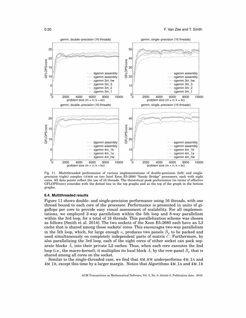
0:30 F. Van Zee and T. Smith
0 2000 4000 6000 8000 100000
5
10
15
20
25
problem size (m = n; k = kc)
GF
LO
PS
/core
gemm, double−precision (16 threads)
dgemm assemblyzgemm assemblyzgemm 3m_hw
zgemm 3m_3zgemm 3m_2zgemm 3m_1
0 2000 4000 6000 8000 100000
10
20
30
40
50
problem size (m = n; k = kc)
GF
LO
PS
/core
gemm, single−precision (16 threads)
sgemm assemblycgemm assemblycgemm 3m_hw
cgemm 3m_3cgemm 3m_2cgemm 3m_1
0 2000 4000 6000 8000 100000
5
10
15
20
problem size (m = n; k = kc)
GF
LO
PS
/core
gemm, double−precision (16 threads)
dgemm assemblyzgemm assembly
zgemm 4m_1b
zgemm 4m_1azgemm 4m_hw
0 2000 4000 6000 8000 100000
10
20
30
40
problem size (m = n; k = kc)
GF
LO
PS
/core
gemm, single−precision (16 threads)
sgemm assemblycgemm assembly
cgemm 4m_1b
cgemm 4m_1acgemm 4m_hw
Fig. 11. Multithreaded performance of various implementations of double-precision (left) and single-precision (right) complex GEMM on two Intel Xeon E5-2680 “Sandy Bridge” processors, each with eightcores. All data points reflect the use of 16 threads. The theoretical peak performance (in terms of effectiveGFLOPS/core) coincides with the dotted line in the top graphs and as the top of the graph in the bottomgraphs.
6.4. Multithreaded resultsFigure 11 shows double- and single-precision performance using 16 threads, with onethread bound to each core of the processor. Performance is presented in units of gi-gaflops per core to provide easy visual assessment of scalability. For all implemen-tations, we employed 2-way parallelism within the 5th loop and 8-way parallelismwithin the 3rd loop, for a total of 16 threads. This parallelization scheme was chosenas follows [Smith et al. 2014]. The two sockets of the Xeon E5-2680 each have an L3cache that is shared among those sockets’ cores. This encourages two-way parallelismin the 5th loop, which, for large enough n, produces two panels Bp to be packed andused simultaneously on completely independent parts of matrix C. Furthermore, byalso parallelizing the 3rd loop, each of the eight cores of either socket can pack sep-arate blocks Ai into their private L2 caches. Thus, when each core executes the 2ndloop (i.e., the macro-kernel), it multiplies its local block Ai by the row-panel Bp that isshared among all cores on the socket.
Similar to the single-threaded case, we find that 4M HW underperforms 4M 1A and4M 1B, except this time by a larger margin. Notice that Algorithms 4M 1A and 4M 1B
ACM Transactions on Mathematical Software, Vol. 0, No. 0, Article 0, Publication date: 2016.

Implementing high-performance complex matrix multiplication via the 3m and 4m methods 0:31
reuse micro-tiles of C from the L1 and L2 caches, respectively, while in 4M HW, whichexecutes in four phases, the F.E. of C are almost never reused from any level of cache.This helps explain the performance shortfall in both the single- and multithreadedcases. We suspect that the much larger shortfall that manifests in the multithreadedcase is due to the system’s memory bandwidth becoming saturated as all 16 threadsvie to update their independent micro-tiles nearly simultaneously.
The double-precision results for 4M 1A and 4M 1B once again fall within 10% of thebenchmark real domain implementation. Surprisingly, in the single-precision case, the4M 1A and 4M 1B implementations track closely with the performance of their realGEMM benchmark.
In general, multithreaded 3M implementations perform somewhat more poorly rel-ative to the single-threaded case. This is likely due to the additional memops consti-tuting a higher percentage of overall runtime cost (relative to 4M), which more quicklyleads to memory bandwidth saturation.
7. FURTHER DISCUSSION7.1. Unifying ObservationsIn light of our theoretical analyses and empirical results, we now offer a series ofobservations which, taken together, begin to condense and unify some of the findingsof this article.
7.1.1. Variance in memops explains relative performance. All 3M and 4M algorithms executethe same number of flops28 as the other algorithms within their respective families,and so each algorithm’s performance relative to others in its family depends on thenumber (and circumstance, which we will comment upon shortly) of memops executed.Tables I and III reveal that the level at which 3M or 4M is applied determines thetotal number of F.E. memops required. In the case of 3M, the loop level determinesthe F.E. memop count in two ways. First, the targeted loop determines the packingstrategy, which sometimes requires blocksize scaling in order to avoid over-occupyingthe various levels of cache. Second, the loop being targeted for 3M determines whetherthe computation of SA and SB can be fused with the packing of Ai and Bp. Blocksizescaling causes the total number of memops to increase, while fusing the computationof SA and SB with packing causes the total number of memops to decrease. In the caseof 4M, only the former effect is applicable. This, combined with a less drastic blocksizescaling factor, results in less variation of F.E. memops across 4M algorithms.
7.1.2. A spectrum of algorithms. Algorithm 4M HW moves each fundamental element ofA, B, and C from main memory to the L1 cache a total of four times each—twice for the4M method, and twice due to incidental spatial (i.e. cache line) proximity—per rank-kC update. And of the reusable elements that are packed to Ai and Bp, none are everreused across calls to RGEMM. Thus, 4M HW makes poor use of each cache line that ismoved through the cache hierarchy.
Algorithm 4M 1A moves each fundamental element of A, B, and C from main mem-ory to the L1 cache only once per rank-kC update. Furthermore, only elements thatare needed are moved; there is virtually no excess data movement due to spacial prox-imity. And as packed micro-panels of Ai and Bp are moved into the L1 cache, they arereused from the L1 cache. Thus, 4M 1A makes very efficient use of each cache line thatis moved through the cache hierarchy.
28In this hypothetical accounting of flops, we assume that the workspace optimization is employed for 3M,and thus the flops involved in the formation of SA and reuse of W r,W i is constant across all 3M algorithmslisted in Table I.
ACM Transactions on Mathematical Software, Vol. 0, No. 0, Article 0, Publication date: 2016.

0:32 F. Van Zee and T. Smith
We can observe, then, that 4M-based algorithms exist along a spectrum with the fol-lowing trade-off properties: (1) The higher the 4M method is applied, the lower the effi-ciency of data movement through the caches, and the lower the 4M method is applied,the higher the efficiency of data movement29; (2) Higher applications can use largerprimitives, while lower applications must use smaller primitives. Larger primitivestend to require fewer modifications to the underlying matrix multiplication frameworkbecause they hide details (particularly with regards to packing and multithreading)that surface when using smaller primitives.30
Notice that data efficiency in the context of 3M is somewhat different. 3M inherentlydoes not reuse any input data beyond that which is already prescribed by the matrixmultiplication algorithm. And we suspect that the total number of F.E. memops re-quired, which exhibits greater variation within the 3M family, generally has a greatereffect on performance than the degree of redundant cache line movements. For exam-ple, our empirical results suggest that, at least in the (important) case of-kC update,the excessive number of F.E. memops incurred by 3M 1 outweighs the combined ben-efit of accessing operands A, B, and C only once each and reusing micro-panels of Ai
and Bp from the L1 cache.
7.1.3. The conventional approach: a special case. The conventional approach discussedin Section 3 corresponds to the special case whereby 4M is applied at the scalar level,within a single rank-1 update of the micro-kernel’s loop. This special case resides at thelowest end of the spectrum of 4M algorithms. Here, efficiency is maximized, as real andimaginary elements are reused only once they have been moved into registers, wherethey are computed upon by an extremely small primitive: a single vector instruction.The cost of this efficiency, though, is that some form of swizzling must be performedat the sub-vector level, sometimes resulting in the programming difficulties suggestedby Figure 2 (right). Note that in the cases of higher level applications (e.g. 4M 1A andhigher), swizzling is somewhat implicit, and is analogous to the referencing of differentreal or imaginary sub-regions of A and B when calling the primitive defined for thatlevel. Of course, this implicit swizzling is not entirely “free” since it often requiresthe data to be rearranged in advance. However, it can be mostly free if packing mustoccur anyway, as is the case with several mid-to-lower level applications of 4M, andwhatever overhead is incurred in the modified packing operation is amortized overplenty of floating-point operations.
7.1.4. The impact of storage. Another contributing factor to the performance of complexmatrix multiplication, one might argue, is actually in the storage of complex numbers.The traditional, interleaved pair-wise storage of real and imaginary values increasesthe potential efficiency of data movement from main memory to registers, and alsounlocks the potential to reuse that data from registers, but the price of realizing thoseefficiencies is assembly-level swizzling. If complex numbers were stored in such a waythat did not favor complex arithmetic being performed in registers, the alternativemethods based on real primitives would be more obvious. Also, the task of express-ing (programming) complex micro-kernels simplifies greatly, as demonstrated by algo-rithm 4M 1A, if we simply forgo pursuit of the best-case scenario of reusing F.E. fromregisters, and instead settle for reuse from the L1 cache. Granted, with this trade-offcomes lower performance. But evidence suggests that the primary cause behind the
29Here, a “higher” or “lower” level application of 4M (or 3M) refers to the targeted loop’s relative positionwithin the overall matrix multiplication algorithm, as depicted in Figure 1.30One exception to this, however, is when 4M is applied a the very lowest level, just outside the micro-kernel.In this case, code changes can remain hidden (within the virtual micro-kernels) and thus those algorithmsrepresent a programming “sweet spot” within the BLIS framework.
ACM Transactions on Mathematical Software, Vol. 0, No. 0, Article 0, Publication date: 2016.

Implementing high-performance complex matrix multiplication via the 3m and 4m methods 0:33
performance drag on 4M algorithms is not reusing F.E. from a more distant level ofcache, but rather the doubling or quadrupling of memops on C, combined with thenon-contiguous nature of those data accesses (which also precludes use of most vectorload and store instructions).31 If there existed an induced method that did not incursuch high costs when updating C, that induced method might perform competitivelywith conventional implementations. Indeed, 4M-based algorithms would be able to up-date C much more efficiently if complex matrices were stored with real and imaginaryparts divided into separate (contiguous row- or column-stored) matrices.32 This sepa-rated storage format would allow the underlying real micro-kernel to always use vectorload and store instructions when accessing the output matrix, thus (largely) avoidingthe performance penalty incurred when accessing only real or only imaginary values.However, this storage scheme is relatively unconventional within the HPC commu-nity, while the traditional interleaved format is quite entrenched. Therefore, it wouldbe unreasonable to expect applications to adapt.
Given these realities, we are left to conclude that, if there exists a better solution, itwill likely not be found through the 4M method.
7.2. Progress and the (challenging) path forwardThe 4M method comes with concrete benefits. It allows developers to focus on fewer andsimpler micro-kernels—reducing coding and maintenance burdens both because thereis less code, and also because that remaining code tends to be more easily expressedin assembly language. And it builds on existing kernels, allowing it to be encodedportably within a BLAS-like framework such as BLIS, where it extends to any level-3 operation with only modest effort. Our experience thus far suggests that 4M caninduce “placeholder” implementations that deliver acceptable (even if short of optimal)performance, which may still be of value in situations where time, resources, and/orexpertise is limited.
Unfortunately, the 4M family of induced algorithms also collectively exhibit real lim-itations which appear inherent in nature. Any future work in this area will be forcedto confront these challenges, or find novel ways of circumventing them altogether:
— Number of calls to primitive. If we assume that virtual micro-kernels are em-ployed to hide implementation details, instantiating 4M algorithms such as 4M 1Acan result in close to a 400% increase in function call overhead relative to a conven-tional assembly-based code. Algorithm 4M H fares even worse with an 800% increase.The small amount of logic present in virtual micro-kernels may also contribute no-ticeable overhead. These extra costs become an issue when they cannot be amortizedacross a sufficient number of floating-point operations, either because the costs them-selves are large or because the L1 cache size limits kC , and thus the number of cyclesworth of computation that can be performed by a single micro-kernel call.
— Inefficient reuse of input data from A, B, and C. Higher and mid-level appli-cations of 4M inefficiently move data from the input matrices through the memoryhierarchy, only to let those elements be evicted from cache before they are reused.
31This observation makes sense when one considers that doubling or quadupling the memop cost on theinput operands (or their packed equivalents) represents a lower order term, mkC + kCn, compared to thepotentially much larger impact from increasing memops on the m× n output matrix C.32The 3M method has a similar affinity towards separate storage of real and imaginary parts. Except sincethe goal of 3M is to reuse intermediate terms, extra memory operations (outside of the micro-kernel) areunavoidable, even if they are performed efficiently via vector instructions. By contrast, separating com-plex matrices into real and imaginary matrices would benefit 4M algorithms by avoiding workspace-relatedmemops and ensuring that the remaining memops on C can execute via vector instructions.
ACM Transactions on Mathematical Software, Vol. 0, No. 0, Article 0, Publication date: 2016.

0:34 F. Van Zee and T. Smith
Only the lowest level algorithms reuse real and imaginary F.E. once they have beenmoved into cache.
— Non-contiguous output to C. 4M-based algorithms must, at some level, updateonly the real and then only the imaginary parts of the output matrix, twice each,which tends to incur a non-trivial increase in runtime cost. Long-term trends inthis area are not favorable to 4M: First, as vector register lengths are extended withnewer architectures and instruction sets, the relative cost of updating individual realor imaginary values will only grow; Second, the cost of memory access relative to thecost of floating-point computation will likely continue its upward trajectory, furthermagnifying the cost of repeatedly accessing the micro-tile of C.
— Reduction of kC . Some algorithms, such as 4M 1A, may require reducing the kCblocksize to maintain cache footprints of packed matrices Ai and Bp as well as indi-vidual micro-panels within those matrices. This causes the real domain micro-kernelto be called on micro-panels with k dimensions that are, at best, half their optimalsize. Consequently, fewer flops are executed per update of C, which means a largerfraction of total runtime is spent accessing elements of the output matrix, thus erod-ing performance.
— Framework accommodation. Many 4M algorithms would require significant anddisruptive changes to BLIS’s underlying code. This effect would likely hold even forother frameworks, because those changes to the framework stem from changes to thematrix multiplication algorithm itself. Ideally, this algorithmic specialization wouldbe avoided.
— Interference with multithreading. Some applications of 4M, particularly those tohigh- and mid-level loops, complicate (or prevent) the ability to express an ideal par-titioning of work and data for many-threaded parallelism, as with Algorithm 4M HW.
— Non-applicability to two-operand operations. Higher level applications, such as4M HW, cannot be used to implement TRMM or TRSM without first making workspace-expensive, performance-degrading copies of the input/output operand B.
These issues conspire to limit (to varying degrees) the achievable performance of4M-based algorithm—a shortfall some may find unacceptable.
8. CONCLUSIONSWe began the article with a brief overview of the conventional approach to implement-ing matrix multiplication in the complex domain. Then, we investigated the 3M methodand provided a detailed analysis of the method’s applicability to each loop within acommonly accepted algorithm for matrix multiplication, exposing several variants inthe process. The more general-purpose 4M method was also discussed, accompaniedby an abbreviated analysis of a select set of possible algorithms. Decent performancewas observed on a modern Intel system. Finally, we identified key familial propertiesof the 3M and 4M algorithms, and summarized their benefits and limitations.
We conclude that while the 3M method can yield effective performance that exceedsthe peak of the machine, some may be wary of its distinct numerical properties. The4M method does not forfeit any numerical advantage over the conventional approach,but often lags slightly behind its real domain benchmarks. Given that conventionally-implemented complex matrix multiplication typically slightly exceeds that of its realdomain counterpart, this lag may be troublesome to many. Still, 4M provides a family ofbackstop solutions—a lower bound on attainable complex performance in the absenceof a complex kernel. Developing an induced method that builds on the performance of4M should be the focus of future work.
ACM Transactions on Mathematical Software, Vol. 0, No. 0, Article 0, Publication date: 2016.

Implementing high-performance complex matrix multiplication via the 3m and 4m methods 0:35
ACKNOWLEDGMENTS
We kindly thank Tze Meng Low for participating in early performance analysis. We also thank the TexasAdvanced Computing Center for providing access to the the Intel Xeon “Stampede” compute cluster on whichSandy Bridge performance data was gathered.33
REFERENCESAGULLO, E., BOUWMEESTER, H., DONGARRA, J., KURZAK, J., LANGOU, J., AND ROSENBERG, L. 2010.
Towards an efficient tile matrix inversion of symmetric positive definite matrices on multicore architec-tures.
AGULLO, E., DEMMEL, J., DONGARRA, J., HADRI, B., KURZAK, J., LANGOU, J., LTAIEF, H., LUSZCZEK, P.,AND TOMOV, S. 2009. Numerical linear algebra on emerging architectures: The PLASMA and MAGMAprojects. Journal of Physics: Conference Series 180.
AMD. 2012. AMD Core Math Library. http://developer.amd.com/tools/cpu/acml/pages/default.aspx.ANDERSON, E., BAI, Z., BISCHOF, C., BLACKFORD, L. S., DEMMEL, J., DONGARRA, J. J., CROZ, J. D.,
HAMMARLING, S., GREENBAUM, A., MCKENNEY, A., AND SORENSEN, D. 1999. LAPACK Users’ guide(third ed.). Society for Industrial and Applied Mathematics, Philadelphia, PA, USA.
CHOI, J., DONGARRA, J. J., POZO, R., AND WALKER, D. W. 1992. ScaLAPACK: A scalable linear algebralibrary for distributed memory concurrent computers. In Proceedings of the Fourth Symposium on theFrontiers of Massively Parallel Computation. IEEE Comput. Soc. Press, 120–127.
DEMMEL, J. W. AND HIGHAM, N. J. 1992. Stability of block algorithms with fast level-3 BLAS. ACM Trans.Math. Soft. 18, 3, 274–291.
DONGARRA, J., BUNCH, J., MOLER, C., AND STEWART, G. 1979. LINPACK Users’ Guide. Society for Indus-trial and Applied Mathematics, Philadelphia.
DONGARRA, J. J., DU CROZ, J., HAMMARLING, S., AND DUFF, I. 1990. A set of level 3 basic linear algebrasubprograms. ACM Trans. Math. Soft. 16, 1, 1–17.
DONGARRA, J. J., LUSZCZEK, P., AND PETITET, A. 2003. The LINPACK benchmark: Past, present, andfuture. concurrency and computation: Practice and experience. Concurrency and Computation: Practiceand Experience 15, 9, 803–820.
GOTO, K. AND VAN DE GEIJN, R. 2008a. Anatomy of high-performance matrix multiplication. ACM Trans.Math. Soft. 34, 3, 12:1–12:25.
GOTO, K. AND VAN DE GEIJN, R. 2008b. High-performance implementation of the level-3 BLAS. ACMTrans. Math. Soft. 35, 1, 1–14.
HIGHAM, N. J. 1990. Exploiting fast matrix multiplication within the level 3 BLAS. ACM Trans. Math.Soft. 16, 4, 352–368.
HIGHAM, N. J. 1992. Stability of a method for multiplying complex matrices with three real matrix multi-plications. SIAM J. Matrix Anal. App. 13, 3, 681–687.
IBM. 2012. Engineering and Scientific Subroutine Library. http://www.ibm.com/systems/software/essl/.INTEL. 2014. Math Kernel Library. http://developer.intel.com/software/products/mkl/.KNUTH, D. E. 1981. The Art of Computer Programming, Volume 2: Seminumerical Algorithms, Second
Edition. Addison-Wesley, Reading, MA, USA.LOW, T. M., IGUAL, F. D., SMITH, T. M., AND QUINTANA-ORTI, E. S. 2016. Analytical modeling is enough
for high-performance BLIS. ACM Trans. Math. Soft. 43, 2, 12:1–12:18.POULSON, J., MARKER, B., VAN DE GEIJN, R. A., HAMMOND, J. R., AND ROMERO, N. A. 2013. Elemental:
A new framework for distributed memory dense matrix computations. ACM Trans. Math. Softw. 39, 2,13:1–13:24.
SMITH, T. M., VAN DE GEIJN, R. A., SMELYANSKIY, M., HAMMOND, J. R., AND VAN ZEE, F. G. 2014.Anatomy of high-performance many-threaded matrix multiplication. In Proceedings of the 28th IEEEInternational Parallel & Distributed Processing Symposium (IPDPS).
STRASSEN, V. 1969. Gaussian elimination is not optimal. Numerische Mathematik 13, 4, 354–356.Top500 2015. Top 500 supercomputer sites. http://www.top500.org/.VAN ZEE, F. G., CHAN, E., VAN DE GEIJN, R., QUINTANA-ORTI, E. S., AND QUINTANA-ORTI, G. 2009.
The libflame library for dense matrix computations. IEEE Computation in Science & Engineering 11, 6,56–62.
33The Stampede system was funded by the National Science Foundation via Award ACI-1134872.
ACM Transactions on Mathematical Software, Vol. 0, No. 0, Article 0, Publication date: 2016.

0:36 F. Van Zee and T. Smith
VAN ZEE, F. G., SMITH, T., IGUAL, F. D., SMELYANSKIY, M., ZHANG, X., KISTLER, M., AUSTEL, V., GUN-NELS, J., LOW, T. M., MARKER, B., KILLOUGH, L., AND VAN DE GEIJN, R. A. 2016. The BLIS frame-work: Experiments in portability. ACM Trans. Math. Soft. 42, 2, 12:1–12:19.
VAN ZEE, F. G. AND VAN DE GEIJN, R. A. 2015. BLIS: A framework for rapidly instantiating BLAS func-tionality. ACM Trans. Math. Soft. 41, 3, 14:1–14:33.
WHALEY, R. C. AND DONGARRA, J. J. 1998. Automatically tuned linear algebra software. In Proceedings ofSC’98.
XIANYI, Z., QIAN, W., AND YUNQUAN, Z. 2012. Model-driven level 3 BLAS performance optimization onLoongson 3A processor. In IEEE 18th International Conference on Parallel and Distributed Systems(ICPADS).
Received May 2015; revised March 2017; accepted December 2017
ACM Transactions on Mathematical Software, Vol. 0, No. 0, Article 0, Publication date: 2016.