MPRAMunich Personal RePEc Archive

Active Hedging Greeks of an OptionsPortfolio integrating churning andminimization of cost of hedging usingQuadratic & Linear Programing

Sinha, Pankaj; Gupta, Akshay and Mudgal, Hemant

Faculty of Management Studies, University of Delhi, Faculty

of Management Studies, University of Delhi, Faculty of

Management Studies, University of Delhi

02. October 2010

Online at http://mpra.ub.uni-muenchen.de/25707/

MPRA Paper No. 25707, posted 07. October 2010 / 11:45

ActiveHedgingGreeksofanOptionsPortfoliointegratingchurningand

minimizationofcostofhedgingusingQuadratic&LinearPrograming

Pankaj Sinha, Akshay Gupta and Hemant Mudgal

Faculty of Management Studies, University of Delhi, Delhi

Abstract

This paper proposes a methodology for active hedging Greeks of an option portfolio integrating

churning and minimization of cost of hedging. In the first section, hedging strategy is implemented

by taking positions in other available options, while simultaneously minimizing the net premium

paid for the hedging and then churning the portfolio to take into account the changed value of

Greeks in the new portfolio. In the second section, the paper extends the model to incorporate the

transaction cost while hedging the portfolio and churning it in Indian Scenario. Both constant and

nonlinear shape of transaction cost has been considered as per the Security Transaction Tax and

Brokerage charges in India. A quadratic programming has been presented which has been

approximated by a linear programming solution. The prototype software has been developed in

MS Excel using Visual Basic.

1. Introduction

Options are one of the most essential instruments being used by the hedgers to reduce the volatility of their

portfolio. However options themselves are volatile. The change in the value of option portfolio can be

described using the Greek variables Delta, Gamma, Vega, Theta and Rho. Due consideration to these values is

essential to formulate any hedging strategy using options portfolio. This is reflected in the research done by

Papahristodoulou [1] who presented a linear programming model to hedge options while incorporating the

Greeks so that one doesn’t need to track the movement of option portfolio with the underlying stocks.

Horasanlı [2] is his work extended the above model to incorporate multi-asset portfolio of options and stocks.

In the past Hull [3] and Rendleman [4] have also discussed ways to hedge an option portfolio. Sinha & Johar

[5] presents a model to hedge Greeks of an existing portfolio by making use of the other available options in

the market while minimizing the premium paid for the construction of hedge.

There are two things which haven’t been discussed in the above mentioned references. Firstly a static view of

portfolio has been considered and secondly transaction costs have been ignored. The value of Greeks changes

continuously over a period of time and hence there is a need to rebalance the portfolio to incorporate the

changed value of Greeks while taking the previous hedged portfolio as input. Transaction costs can play a

significant part in determining whether the benefits of hedging are more than the costs of hedging or not. In

the subsequent sections, we extend the methodology of Sinha & Johar [5] to rebalance the option portfolio

while taking into account the changed value of Greeks and we have further augmented our model by

incorporating transaction costs in Indian Scenario. We present a quadratic programming solution which has

been approximated by a linear programming solution for which a prototype has been developed using MS-

Excel and Visual Basic.

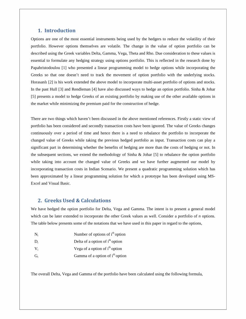
2. Greeks Used & Calculations

We have hedged the option portfolio for Delta, Vega and Gamma. The intent is to present a general model

which can be later extended to incorporate the other Greek values as well. Consider a portfolio of n options.

The table below presents some of the notations that we have used in this paper in regard to the options,

Ni Number of options of ith option

Di Delta of a option of ith option

V i Vega of a option of ith option

Gi Gamma of a option of ith option

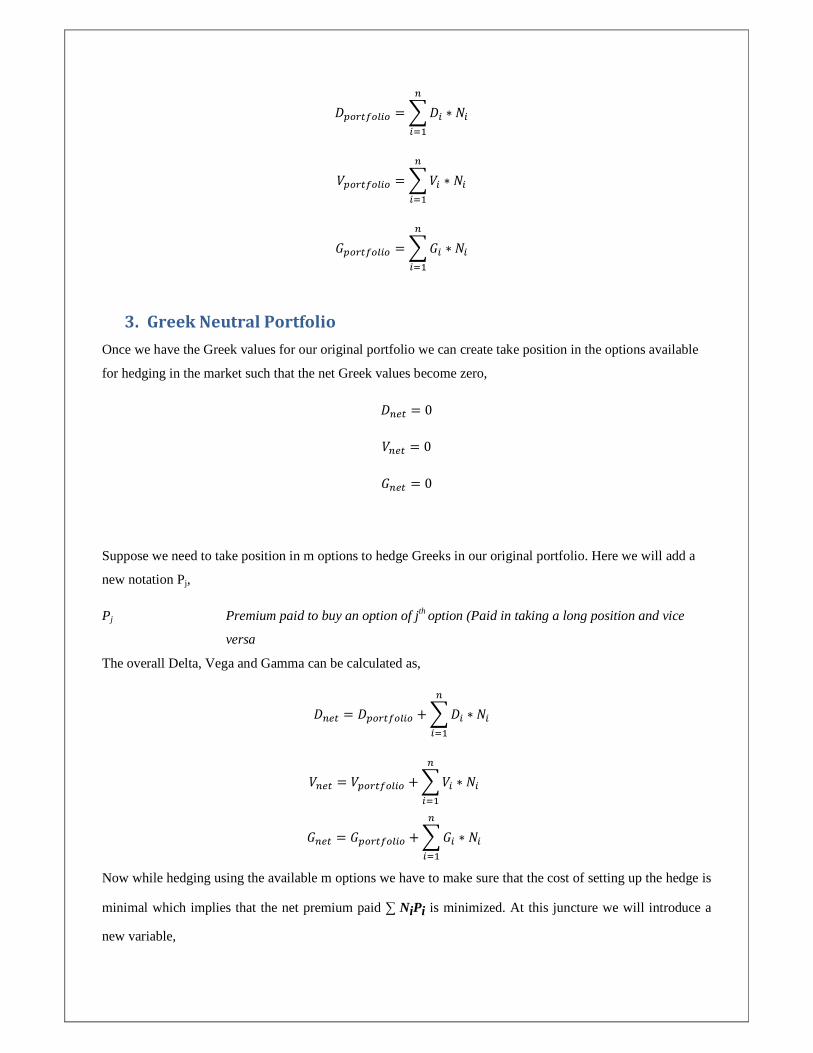
The overall Delta, Vega and Gamma of the portfolio have been calculated using the following formula,

���������� = �� ∗ ��

���

���������� = �� ∗ ��

���

���������� = �� ∗ ��

���

3. Greek Neutral Portfolio

Once we have the Greek values for our original portfolio we can create take position in the options available

for hedging in the market such that the net Greek values become zero,

� �� = 0

� �� = 0

� �� = 0

Suppose we need to take position in m options to hedge Greeks in our original portfolio. Here we will add a

new notation Pj,

Pj Premium paid to buy an option of jth option (Paid in taking a long position and vice

versa

The overall Delta, Vega and Gamma can be calculated as,

� �� = ���������� + �� ∗ ��

���

� �� = ���������� + �� ∗ ��

���

� �� = ���������� + �� ∗ ��

���

Now while hedging using the available m options we have to make sure that the cost of setting up the hedge is

minimal which implies that the net premium paid ∑ NiPi is minimized. At this juncture we will introduce a

new variable,

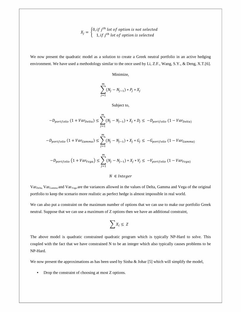
�� =�0, ������� ���! ��"�#"� #$�$% $&1, ������� ���! ��"�##$�$% $&

We now present the quadratic model as a solution to create a Greek neutral portfolio in an active hedging

environment. We have used a methodology similar to the once used by Li, Z.F., Wang, S.Y., & Deng, X.T.[6].

Minimize,

(�� − ��*�+

���) ∗ -� ∗ ��

Subject to,

−����������(1 + �./0���1) ≤ (�� − ��*�+

���) ∗ �� ∗ �� ≤−����������(1 − �./0���1)

−����������(1 + �./31++1) ≤ (�� − ��*�+

���) ∗ �� ∗ �� ≤−����������(1 − �./31++1)

−���������� 41 + �./5�617 ≤ (�� − ��*�+

���) ∗ �� ∗ �� ≤−����������(1 − �./5�61)

� ∈ 9" $:$/

VarDelta, VarGamma and VarVega are the variances allowed in the values of Delta, Gamma and Vega of the original

portfolio to keep the scenario more realistic as perfect hedge is almost impossible in real world.

We can also put a constraint on the maximum number of options that we can use to make our portfolio Greek

neutral. Suppose that we can use a maximum of Z options then we have an additional constraint,

�� ≤ ;

The above model is quadratic constrained quadratic program which is typically NP-Hard to solve. This

coupled with the fact that we have constrained N to be an integer which also typically causes problems to be

NP-Hard.

We now present the approximations as has been used by Sinha & Johar [5] which will simplify the model,

• Drop the constraint of choosing at most Z options.

• Instead of constraining N to be integers we can use the following constraint to impose variance limits

on N,

<�� − =�>"&(��)< ≤ �./? ∗ ��

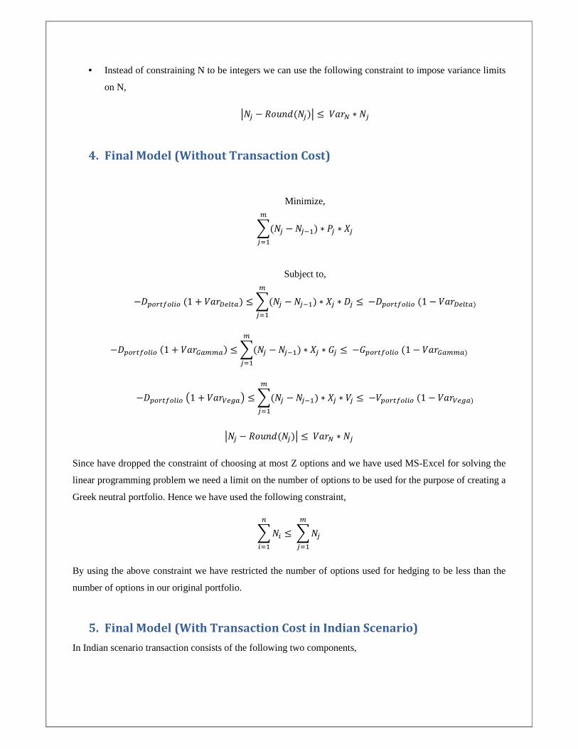
4. Final Model (Without Transaction Cost)

Minimize,

(�� − ��*�+

���) ∗ -� ∗ ��

Subject to,

−����������(1 + �./0���1) ≤ (�� − ��*�+

���) ∗ �� ∗ �� ≤−����������(1 − �./0���1)

−����������(1 + �./31++1) ≤ (�� − ��*�+

���) ∗ �� ∗ �� ≤−����������(1 − �./31++1)

−���������� 41 + �./5�617 ≤ (�� − ��*�+

���) ∗ �� ∗ �� ≤−����������(1 − �./5�61)

<�� − =�>"&(��)< ≤ �./? ∗ ��

Since have dropped the constraint of choosing at most Z options and we have used MS-Excel for solving the

linear programming problem we need a limit on the number of options to be used for the purpose of creating a

Greek neutral portfolio. Hence we have used the following constraint,

�� ≤��+

���

���

By using the above constraint we have restricted the number of options used for hedging to be less than the

number of options in our original portfolio.

5. Final Model (With Transaction Cost in Indian Scenario)

In Indian scenario transaction consists of the following two components,

1. Security Transaction Tax (STT) – As per the Finance Act 2004, and modified by Finance Act 2008

(18 of 2008) STT on the transactions executed on the Exchange is as under, NSE[6].

Sale of an option in securities 0.017% Paid by Seller

Sale of an option in securities, where option is exercised 0.125% Paid by Purchaser

Hence STT per option can be considered to be constant and doesn’t change with the number of

contracts and would only depend on the premium paid or received.

2. Brokerage – Brokerage is charged by the various brokers and is often negotiable. Brokerage charges

generally decrease as the volume of the trade increases.

To incorporate transaction cost in the model discussed in the previous section an additional constraint is

provided to limit the transaction cost below a certain value which can be specified by the user. If S is the

maximum amount that the hedger would like to spend on the transaction cost then the additional

constraint for this model is,

(@A + @BCC) ∗ 4�� − ��*�7 ≤ D

6. Illustration

Prototype software was developed using MS-Excel and Visual Basic to solve the above model.

For the purpose of illustration we have used the same original portfolio as used by Papahristodoulou [1]. The

following two sets of Ericsson options were available as of 13th Feb, 2001. The stock price was trading at

SEK 96 at the Stockholm Stock Exchange. The first set of options corresponds to April options (days to expire

were 66) and the second set corresponds to June options (days to expire were 122). The risk free rate of

interest was 6%. Implicit volatility was estimated as 57% for April options and 55% for June options. The

three and six month volatilities were 68% and 65% respectively.

Our aim is to establish a portfolio for a trader who wishes to hedge a portfolio formed using April options, as

per his trading strategy, with June options.

Option Type Number

of Options

Strike Price

Premium Paid & Received

Delta Gamma Vega

Call 0 95 10.25 0.5815 0.01407 15.944 Call 32 100 7.75 0.5118 0.01436 16.279 Call 0 105 6 0.4442 0.01423 16.126 Call 0 110 4.5 0.3816 0.01373 15.563 Call 28 115 3.1 0.3246 0.01295 14.685 Call 0 120 2.5 0.2736 0.01199 13.586

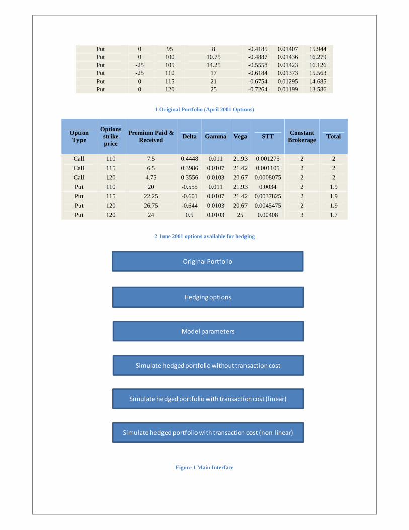
Put 0 95 8 -0.4185 0.01407 15.944 Put 0 100 10.75 -0.4887 0.01436 16.279 Put -25 105 14.25 -0.5558 0.01423 16.126 Put -25 110 17 -0.6184 0.01373 15.563 Put 0 115 21 -0.6754 0.01295 14.685 Put 0 120 25 -0.7264 0.01199 13.586

1 Original Portfolio (April 2001 Options)

Option Type

Options strike price

Premium Paid & Received

Delta Gamma Vega STT Constant

Brokerage Total

Call 110 7.5 0.4448 0.011 21.93 0.001275 2 2

Call 115 6.5 0.3986 0.0107 21.42 0.001105 2 2

Call 120 4.75 0.3556 0.0103 20.67 0.0008075 2 2

Put 110 20 -0.555 0.011 21.93 0.0034 2 1.9

Put 115 22.25 -0.601 0.0107 21.42 0.0037825 2 1.9

Put 120 26.75 -0.644 0.0103 20.67 0.0045475 2 1.9

Put 120 24 0.5 0.0103 25 0.00408 3 1.7

2 June 2001 options available for hedging

Figure 1 Main Interface

Original Portfolio

Hedging options

Simulate hedged portfolio without transaction cost

Simulate hedged portfolio with transaction cost (linear)

Simulate hedged portfolio with transaction cost (non-linear)

Model parameters

1. Without transaction cost

We have constrained the number of options used for hedging to be less than the number of options in the

original portfolio and hence the limit on the number of options which can be used is 110. Now simulating the

hedge without transaction cost for the first time gives us the following results,

The magnified view of the results table is,

Since we haven’t considered the transaction cost in the first simulation hence the transaction cost is zero. The

first row in the table show the various parameters for the option portfolio, the second row show the results

after the second last hedging cycle, the third row show the results after the last hedging cycle, and the last row

show the parameters for the new option portfolio used to hedge the previous portfolio.

Since this is the first simulation the values of the portfolio in the second row is the same as the value in the

first row.

The table below shows the options wise positions that we need to take in order to make our portfolio Greek

neutral,

New options portfolio to be used for hedging

Option

Type Strike Price

Premium Paid/

Received per option

Number of

options

long/short

Call 110 7.5 -54.67275501

Call 115 6.5 -2.661842637

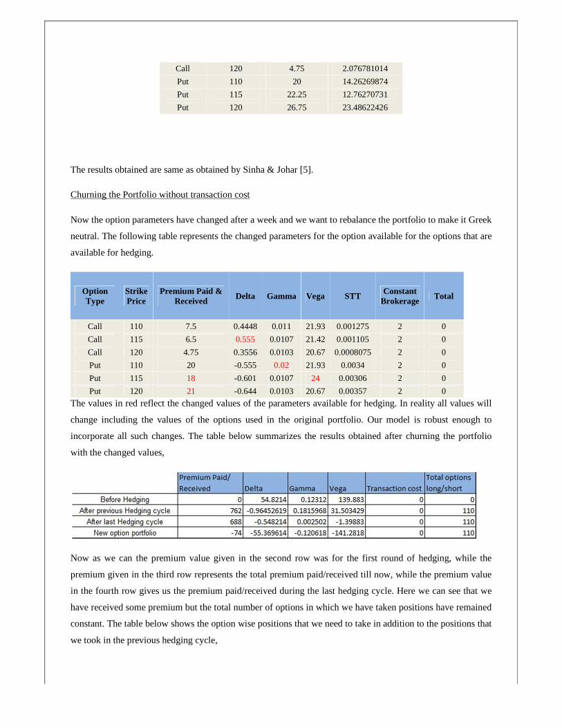
Call 120 4.75 2.076781014

Put 110 20 14.26269874

Put 115 22.25 12.76270731

Put 120 26.75 23.48622426

The results obtained are same as obtained by Sinha & Johar [5].

Churning the Portfolio without transaction cost

Now the option parameters have changed after a week and we want to rebalance the portfolio to make it Greek

neutral. The following table represents the changed parameters for the option available for the options that are

available for hedging.

Option Type

Strike Price

Premium Paid & Received

Delta Gamma Vega STT Constant

Brokerage Total

Call 110 7.5 0.4448 0.011 21.93 0.001275 2 0

Call 115 6.5 0.555 0.0107 21.42 0.001105 2 0

Call 120 4.75 0.3556 0.0103 20.67 0.0008075 2 0

Put 110 20 -0.555 0.02 21.93 0.0034 2 0

Put 115 18 -0.601 0.0107 24 0.00306 2 0

Put 120 21 -0.644 0.0103 20.67 0.00357 2 0

The values in red reflect the changed values of the parameters available for hedging. In reality all values will

change including the values of the options used in the original portfolio. Our model is robust enough to

incorporate all such changes. The table below summarizes the results obtained after churning the portfolio

with the changed values,

Now as we can the premium value given in the second row was for the first round of hedging, while the

premium given in the third row represents the total premium paid/received till now, while the premium value

in the fourth row gives us the premium paid/received during the last hedging cycle. Here we can see that we

have received some premium but the total number of options in which we have taken positions have remained

constant. The table below shows the option wise positions that we need to take in addition to the positions that

we took in the previous hedging cycle,

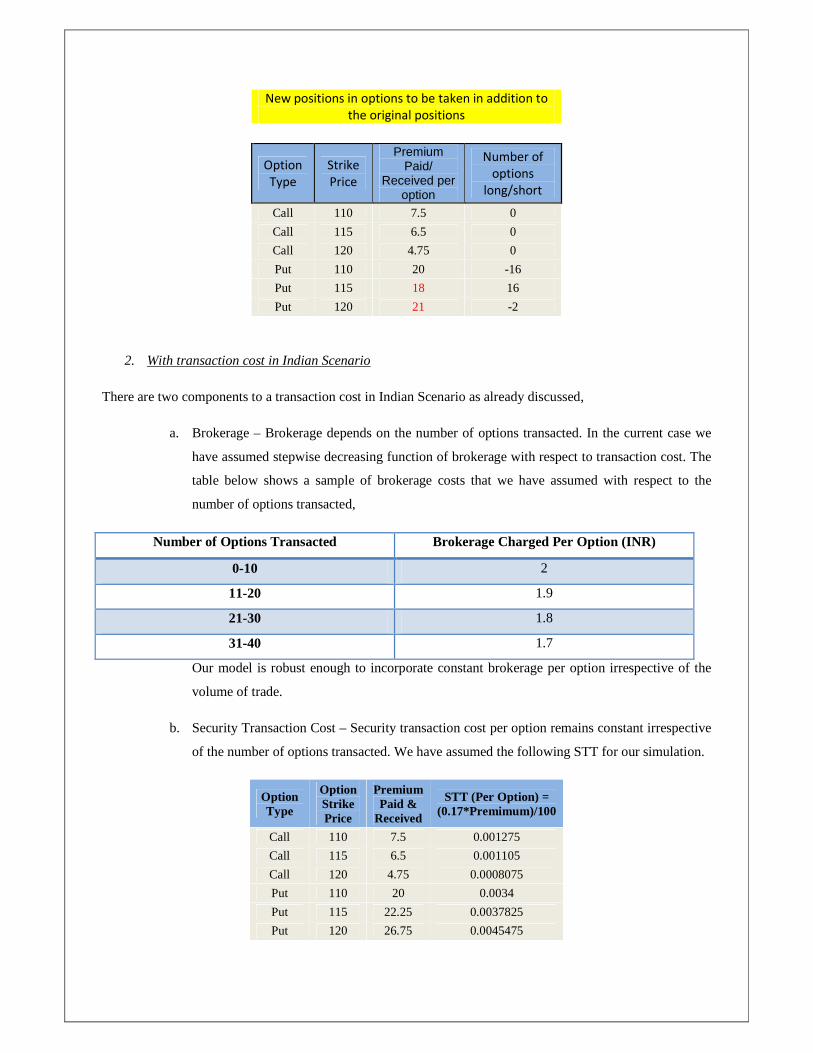
New positions in options to be taken in addition to

the original positions

Option

Type

Strike

Price

Premium Paid/

Received per option

Number of

options

long/short

Call 110 7.5 0

Call 115 6.5 0

Call 120 4.75 0

Put 110 20 -16

Put 115 18 16

Put 120 21 -2

2. With transaction cost in Indian Scenario

There are two components to a transaction cost in Indian Scenario as already discussed,

a. Brokerage – Brokerage depends on the number of options transacted. In the current case we

have assumed stepwise decreasing function of brokerage with respect to transaction cost. The

table below shows a sample of brokerage costs that we have assumed with respect to the

number of options transacted,

Number of Options Transacted Brokerage Charged Per Option (INR)

0-10 2

11-20 1.9

21-30 1.8

31-40 1.7

Our model is robust enough to incorporate constant brokerage per option irrespective of the

volume of trade.

b. Security Transaction Cost – Security transaction cost per option remains constant irrespective

of the number of options transacted. We have assumed the following STT for our simulation.

Option Type

Option Strike Price

Premium Paid &

Received

STT (Per Option) = (0.17*Premimum)/100

Call 110 7.5 0.001275

Call 115 6.5 0.001105

Call 120 4.75 0.0008075

Put 110 20 0.0034

Put 115 22.25 0.0037825

Put 120 26.75 0.0045475

Now we will again consider the same original portfolio and same options available for hedging. However the

difference would be to limit the transaction cost to INR 1000. Simulating the portfolio we get the following

results,

Since the transaction cost limit was set to INR 1000 while to obtain a Greek neutral portfolio only INR 185.2

were required hence the results are similar as in the case of hedging without transaction costs.

Now we will limit the transaction cost to INR 150 and rerun the model from the scratch, i.e. considering the

original portfolio again. We get the following results with the limit,

Now since our transaction cost was limited to INR 150 our Greeks in the hedged portfolio haven’t been

hedged completely and hence showing a more realistic scenario. The options positions that we need to take in

order to hedge our portfolio are,

New positions in options to be taken in addition to

the original positions

Option

Type

Strike

Price

Premium Paid/

Received per lot

Number of

options

long/short

Call 110 7.5 -45

Call 115 6.5 -1

Call 120 4.75 0

Put 110 20 13

Put 115 22.25 13

Put 120 26.75 14

Now we will churn the portfolio again by changing some of the parameters as in the previous case without

transaction costs. The transaction cost has been again given a limit of INR 150. The table below shows the

changed parameter values of the options available for hedging,

Option Type

Option strike price

Premium Paid & Received

Delta Gamma Vega

Call 110 7.5 0.4448 0.011 21.93

Call 115 6.5 0.555 0.0107 21.42

Call 120 4.75 0.3556 0.0103 20.67

Put 110 20 -0.555 0.02 21.93

Put 115 18 -0.601 0.0107 24

Put 120 21 -0.644 0.0103 20.67

Simulating the hedging we get the following results after churning the portfolio,

We can see that the transaction cost in the second round has been INR 117.1 and which is again less than the

limit of INR 150 and the portfolio is almost Greek neutral. The new positions that we need to take in addition

to the original positions are,

New positions in options to be taken in addition to

the original positions

Option

Type

Strike

Price

Premium Paid/

Received per lot

Number of

options

long/short

Call 110 7.5 -9

Call 115 6.5 -3

Call 120 4.75 1

Put 110 20 -13

Put 115 18 28

Put 120 21 -8

Hence we can conclude that the option portfolio can be made Greek neutral using the methodology described

above. In addition to a static view our methodology incorporates an active hedging environment and

transaction costs in Indian Scenario.

7. References

[1] Papahristodoulou, C. (2004). Option strategies with linear programming, European Journal of

Operational Research, 157, 246–256.

[2] Horasanlı, M. (2008). Hedging strategy for a portfolio of options and stocks with linear

programming, Applied Mathematics and Computation, 199, 804–810.

[3] Hull, J. C. (2009). Options, Futures, and Other Derivatives, Prentice Hall.

[4] Rendleman, R. J. (1995). An LP approach to option portfolio selection, Advances in Futures and

Options Research, 8, 31–52.

[5] Sinha, P & Johar, A. (2010). Hedging Greeks for a Portfolio of Options using Linear and Quadratic

Programming, Journal of Prediction Markets. 4(1):17 -26

[6] Li, Z.F., Wang, S.Y., & Deng, X.T. (2000). A linear programming algorithm for optimal portfolio

selection with transaction costs, International Journal of Systems Science, 2000, volume 31, number 1, pages

107 – 117