ASSIGNMENTSPACKET

Assignment 1Article Summary

For this assignment you are asked to read an applied Economics paper (i.e., one using statistical analysis and published in a peer-reviewed Economics journal) of your choosing and summarize its content in a minimum of 1 written page (double-spaced, 12-point font, and 1-inch margins). The purpose of this assignment is to get you started reading papers, summarizing content, and presenting results in front of a group. You will present a 3 minute summary to the class using PowerPoint slides. In your written summary and PowerPoint slides, you need to discuss the following:

1. Why did you choose the article?2. What issue (i.e., theoretical model) does the article address? 3. What data was used in the article and why was this particular data used?4. What empirical model was estimated and what are the main results?5. How might someone extend this line of research?

Some suggestions:

Avoid articles that are so full of mathematics they are unreadable. Note: Most articles in Economics these days contain some degree of mathematics in them. You’re not expected to understand higher-level math. Rather, read the article (especially the introduction, literature summary, and estimation results sections) for key highlights.

Feel free to show me a few articles you are considering. I might be able to steer you towards the most appropriate article.

Your article needs to estimate some sort of econometric (i.e., regression) model.

Assignment 2Practice with Software I

MAKE SURE TO PROVIDE ALL STATISTICAL OUTPUT

For this assignment you are asked to input data into Eviews (or your preferred econometrics package) and perform various tasks. The purpose of this assignment is for you to gain experience working with data, as well as presenting results in tables.

To begin, you need to go to Gallet’s web site (http://www.csus.edu/indiv/g/galletc/) and input the data by clicking on the link labeled GonoData. The data set contains annual California county-level observations for the 2003-2012 period. Because observations vary across county and year, the data set is panel in nature. However, several observations are missing (e.g., there is no data for Alpine County and several years are missing for Sacramento County), making this an “unbalanced” panel data set (consisting of 545 observations). For simplicity, select “unstructured/undated” as the Workfile structure type. Observations on the following variables are contained in the data set:

GONO = Gonorrhea rate (i.e., number of cases per 100,000 population)PUBHLTH = Real per capita spending on public health PHYS = Number of physicians per 1,000 populationP65 = Percent of the population age 65 and olderPDEN = Population density (i.e., population per square mile) PUBLICU = 1 if a CSU or UC campus is located in county i at time t, 0 if notREGION1 = 1 if county i is located in San Francisco Bay Region, 0 if notREGION2 = 1 if county i is located in Southern California (excluding LA) Region, 0 if notREGION3 = 1 if county i is located in Los Angeles Region, 0 if not REGION4 = 1 if county i is located in Central/Southern Farm Region, 0 if notREGION5 = 1 if county i is located in North/Mountain Region, 0 if notREGION6 = 1 if county i is located in Central Valley Region, 0 if not

Note: Each county in California is in one and only one of the 6 regions defined above (e.g., Sacramento County is in Region 6 and not in Regions 1 – 5, while Ventura County is in Region 2 and not in Regions 1 and 3 – 6.

Suppose in the population we believe GONO depends somehow on these variables, and propose three population regression equations, given by:

GONO = β0 + β1PUBHLTH + ε (1)GONO = β0 + β1PUBHLTH + β2PHYS + β3P65 + β4PDEN + β5PUBLICU + ε (2) GONO = β0 + β1PUBHLTH + β2PHYS + β3P65 + β4PDEN + β5PUBLICU + β6REGION1 +

β7REGION2 + β8REGION3 + β9REGION4 + β10REGION5 + ε (3)

Note: Your answers to the sections below need to be typed in Word (double-spaced, 12-point font, and 1-inch margins).

Address the following:

A. In all three equations above, what is the purpose of ε?

B. Regarding the estimation of equation (1), what is the difference between β1 and β̂1?

C. Regarding equation (2), what plausible stories (i.e., hypotheses) can you tell as to how each regressor might affect the regressand in the population? Based on your stories, what do you expect to be the signs of the population parameters (i.e., β1 – β5)?

Hint: Your hypotheses are constructed prior to estimating any regressions. That is, you don’t run regressions and then use the output to form beliefs about the population.

D. Regarding equation (3), why do we not directly include REGION6 in the equation?

E. With the data in Eviews (or your preferred econometrics software package), create a table of descriptive statistics. Specifically, take a look at the template on the next page:1

1 You can go to Gallet’s website, click on the Assignments link, and then easily download the Word file containing this and other tables. You can then copy and paste the templates into your document.

Table 1. Descriptive Statistics

Variables MeanStandardDeviation Minimum Maximum

Dependent Variable:GONO

Independent Variables:

PUBHLTH

PHYS

P65

PDEN

PUBLICU

REGION1

REGION2

REGION3

REGION4

REGION5

REGION6

W

W

W

W

W

W

W

W

W

W

W

W

X

X

X

X

X

X

X

X

X

X

X

X

Y

Y

Y

Y

Y

Y

Y

Y

Y

Y

Y

Y

Z

Z

Z

Z

Z

Z

Z

Z

Z

Z

Z

Z

Note: W, X, Y, and Z are just “place markers” (i.e., they show you where numbers should be entered, down to two decimal places (e.g., 3251.3384 becomes 3251.34, while 12.099 becomes 12.10), such that they align with the variable names in the first column of the table).

Complete this table by providing in the appropriate spaces the mean, standard deviation, minimum, and maximum values of each corresponding variable listed in the table.

F. See the template below for reporting correlation coefficients:

Table 2. Correlation Coefficients

Variables GONO PUBHLTH

PHYS P65 PDEN PUBLICU

GONO 1 A B C D E

PUBHLTH

1 F G H I

PHYS 1 J K L

P65 1 M N

PDEN 1 O

PUBLICU 1

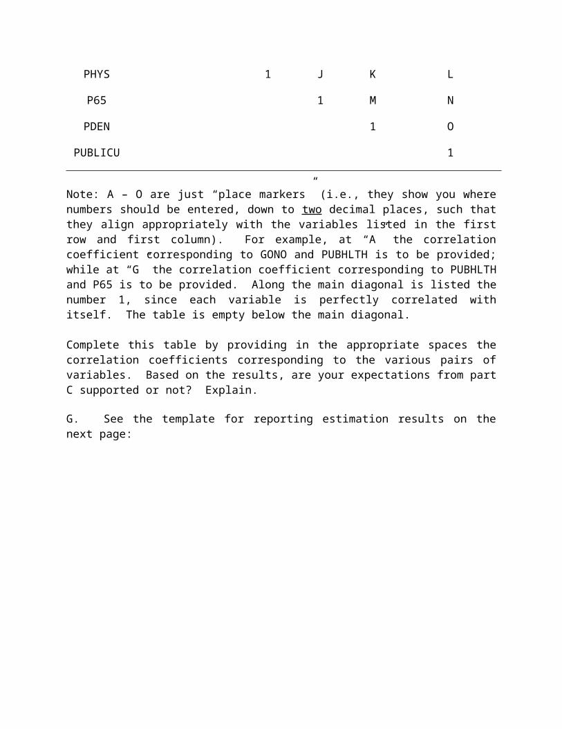
Note: A – O are just “place markers” (i.e., they show you where numbers should be entered, down to two decimal places, such that they align appropriately with the variables listed in the first row and first column). For example, at “A” the correlation coefficient corresponding to GONO and PUBHLTH is to be provided; while at “G” the correlation coefficient corresponding to PUBHLTH and P65 is to be provided. Along the main diagonal is listed the number 1, since each variable is perfectly correlated with itself. The table is empty below the main diagonal.

Complete this table by providing in the appropriate spaces the correlation coefficients corresponding to the various pairs of variables. Based on the results, are your expectations from part C supported or not? Explain. G. See the template for reporting estimation results on the next page:

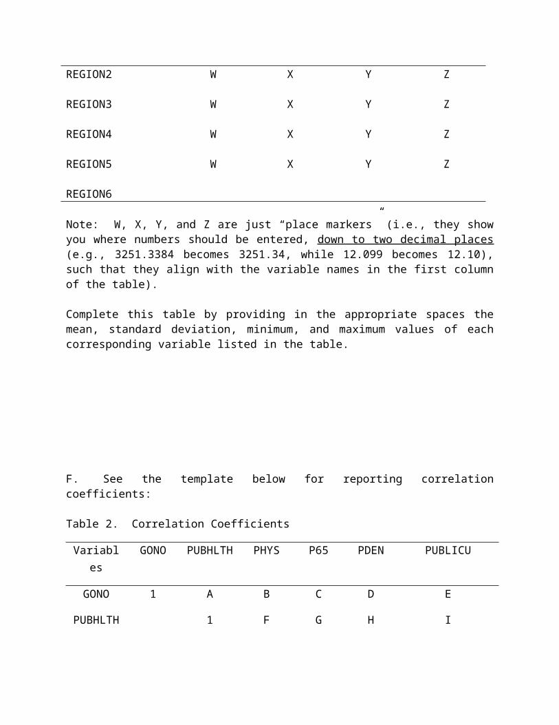
Table 3. Estimation ResultsVariables (1) (2) (3)

Constant

PUBHLTH

PHYS

P65

PDEN

PUBLICU

REGION1

REGION2

REGION3

REGION4

REGION5

A(B)

A(B)

A(B)

A(B)

A(B)

A(B)

A(B)

A(B)

A(B)

A(B)

A(B)

A(B)

A(B)

A(B)

A(B)

A(B)

A(B)

A(B)

A(B)

# obsR2

Adj. R2

CDE

CDE

CDE

Note: Standard errors are in parentheses below coefficient estimates.

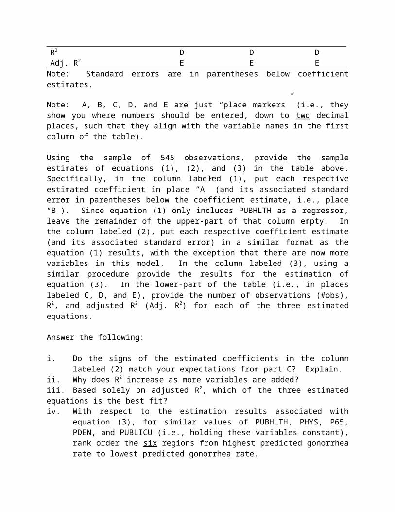
Note: A, B, C, D, and E are just “place markers” (i.e., they show you where numbers should be entered, down to two decimal places, such that they align with the variable names in the first column of the table).

Using the sample of 545 observations, provide the sample estimates of equations (1), (2), and (3) in the table above. Specifically, in the column labeled (1), put each respective estimated coefficient in place “A” (and its associated standard error in parentheses below the coefficient estimate, i.e., place “B”). Since equation (1) only includes PUBHLTH as a regressor, leave the remainder of the upper-part of that column empty. In the column labeled (2), put each respective coefficient estimate (and its associated standard error) in a similar format as the equation (1) results, with the exception that there are now more variables in this model. In the column labeled (3), using a similar procedure provide the results for the estimation of equation (3). In the lower-part of the table (i.e., in places labeled C, D, and E), provide the number of observations (#obs), R2, and adjusted R2 (Adj. R2) for each of the three estimated equations.

Answer the following:

i. Do the signs of the estimated coefficients in the column labeled (2) match your expectations from part C? Explain.

ii. Why does R2 increase as more variables are added?iii. Based solely on adjusted R2, which of the three estimated equations is the best fit? iv. With respect to the estimation results associated with equation (3), for similar values of

PUBHLTH, PHYS, P65, PDEN, and PUBLICU (i.e., holding these variables constant), rank order the six regions from highest predicted gonorrhea rate to lowest predicted gonorrhea rate.

Assignment 3Research Prospectus

For this assignment you are asked to write a research prospectus (2 pages minimum, double-spaced, 12-point font, and 1-inch margins). The purpose of the prospectus is to have you briefly discuss your proposed research topic. Prior to writing the prospectus, you should have read a few studies relevant to your proposed topic so that enough thought has been given to know your project is feasible (i.e., there is relevant data available and the project is neither too narrow nor too broad).

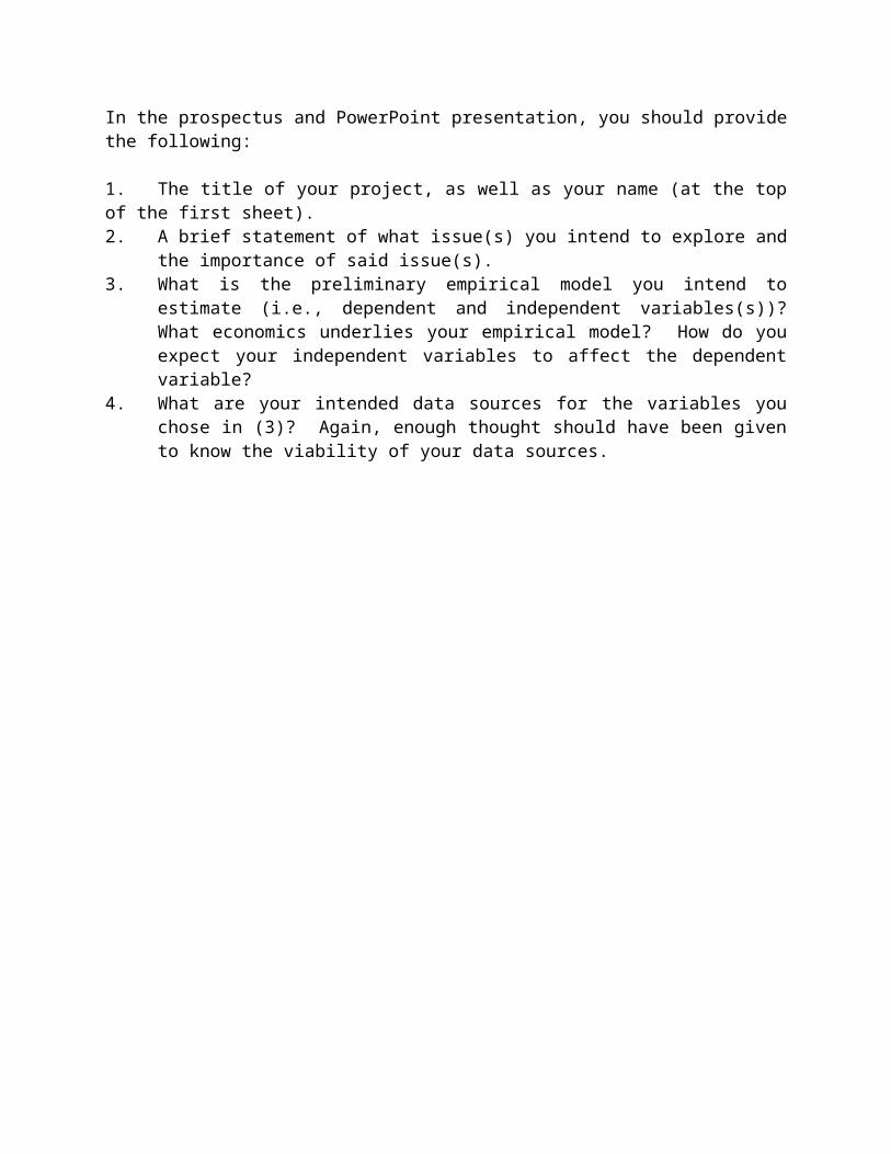
In addition to the written prospectus, you will present a 3-minute PowerPoint presentation of your prospectus to your peers. In the prospectus and PowerPoint presentation, you should provide the following:

1. The title of your project, as well as your name (at the top of the first sheet).2. A brief statement of what issue(s) you intend to explore and the importance of said

issue(s). 3. What is the preliminary empirical model you intend to estimate (i.e., dependent and

independent variables(s))? What economics underlies your empirical model? How do you expect your independent variables to affect the dependent variable?

4. What are your intended data sources for the variables you chose in (3)? Again, enough thought should have been given to know the viability of your data sources.

Assignment 4Practice with Software II

MAKE SURE TO PROVIDE ALL STATISTICAL OUTPUT

For this assignment you are asked to analyze various regression specifications using Eviews (or your preferred econometrics package). The purpose of this assignment is for you to gain further experience estimating regressions, as well as interpreting and presenting results in tables.

To begin, we will work with the same data set used for the Assignment 2 (i.e., the data set labeled GonoData on Gallet’s web site). Recall, we considered three potential population regressions, given by:

GONO = β0 + β1PUBHLTH + ε (1)GONO = β0 + β1PUBHLTH + β2PHYS + β3P65 + β4PDEN + β5PUBLICU + ε (2) GONO = β0 + β1PUBHLTH + β2PHYS + β3P65 + β4PDEN + β5PUBLICU + β6REGION1 +

β7REGION2 + β8REGION3 + β9REGION4 + β10REGION5 + ε (3)

Note: Your answers to the sections below need to be typed in Word (double-spaced, 12-point font, and 1-inch margins).

A. For each of the three equations above, you are to test the significance of the individual estimated coefficients. Specifically, for each coefficient consider the following:

1H0: βi = 0 i = 1, 2,…10HA: βi ≠ 0

Using conventional values of α of 0.01 (i.e., test at the 1% level of significance), 0.05 (i.e., test at the 5% level of significance), and 0.10 (i.e., test at the 10% level of significance), determine which estimated coefficients are significantly different from zero (and at what value of α), as well as which coefficients are insignificantly different from zero.

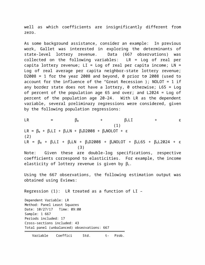
As some background assistance, consider an example: In previous work, Gallet was interested in exploring the determinants of state-level lottery revenue. Data (667 observations) was collected on the following variables: LR = Log of real per capita lottery revenue; LI = Log of real per capita income; LN = Log of real average per capita neighbor-state lottery revenue; D2008 = 1 for the year 2008 and beyond, 0 prior to 2008 (used to account for the influence of the “Great Recession”); NOLOT = 1 if any border state does not have a lottery, 0 otherwise; L65 = Log of percent of the population age 65 and over; and L2024 = Log of percent of the population age 20-24. With LR as the dependent variable, several preliminary regressions were considered, given by the following population regressions:

LR = β0 + β1LI + ε (1)LR = β0 + β1LI + β2LN + β3D2008 + β4NOLOT + ε (2)

LR = β0 + β1LI + β2LN + β3D2008 + β4NOLOT + β5L65 + β6L2024 + ε (3)

Note: Given these are double-log specifications, respective coefficients correspond to elasticities. For example, the income elasticity of lottery revenue is given by β1.

Using the 667 observations, the following estimation output was obtained using Eviews:

Regression (1): LR treated as a function of LI –

Dependent Variable: LRMethod: Panel Least SquaresDate: 10/27/17 Time: 09:00Sample: 1 667Periods included: 17Cross-sections included: 43Total panel (unbalanced) observations: 667

Variable Coefficient Std. Error t-Statistic Prob.

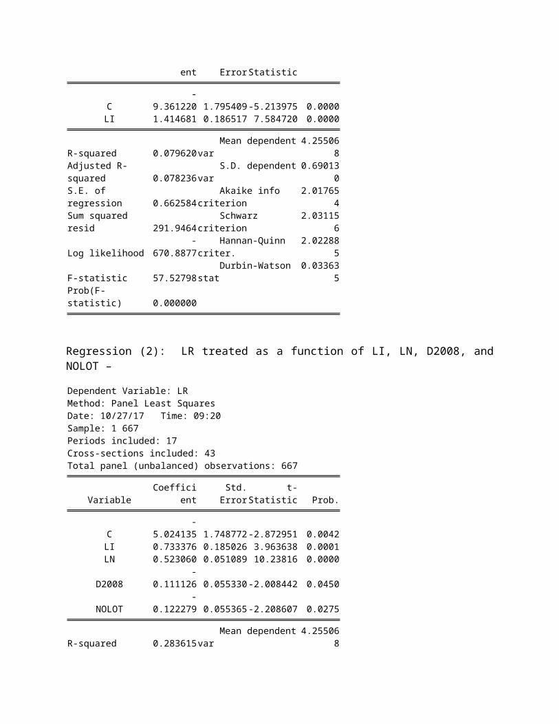
C -9.361220 1.795409 -5.213975 0.0000LI 1.414681 0.186517 7.584720 0.0000

R-squared 0.079620    Mean dependent var 4.255068Adjusted R-squared 0.078236    S.D. dependent var 0.690130S.E. of regression 0.662584    Akaike info criterion 2.017654Sum squared resid 291.9464    Schwarz criterion 2.031156Log likelihood -670.8877    Hannan-Quinn criter. 2.022885F-statistic 57.52798    Durbin-Watson stat 0.033635Prob(F-statistic) 0.000000

Regression (2): LR treated as a function of LI, LN, D2008, and NOLOT –

Dependent Variable: LRMethod: Panel Least SquaresDate: 10/27/17 Time: 09:20Sample: 1 667Periods included: 17Cross-sections included: 43Total panel (unbalanced) observations: 667

Variable Coefficient Std. Error t-Statistic Prob.

C -5.024135 1.748772 -2.872951 0.0042LI 0.733376 0.185026 3.963638 0.0001LN 0.523060 0.051089 10.23816 0.0000

D2008 -0.111126 0.055330 -2.008442 0.0450NOLOT -0.122279 0.055365 -2.208607 0.0275

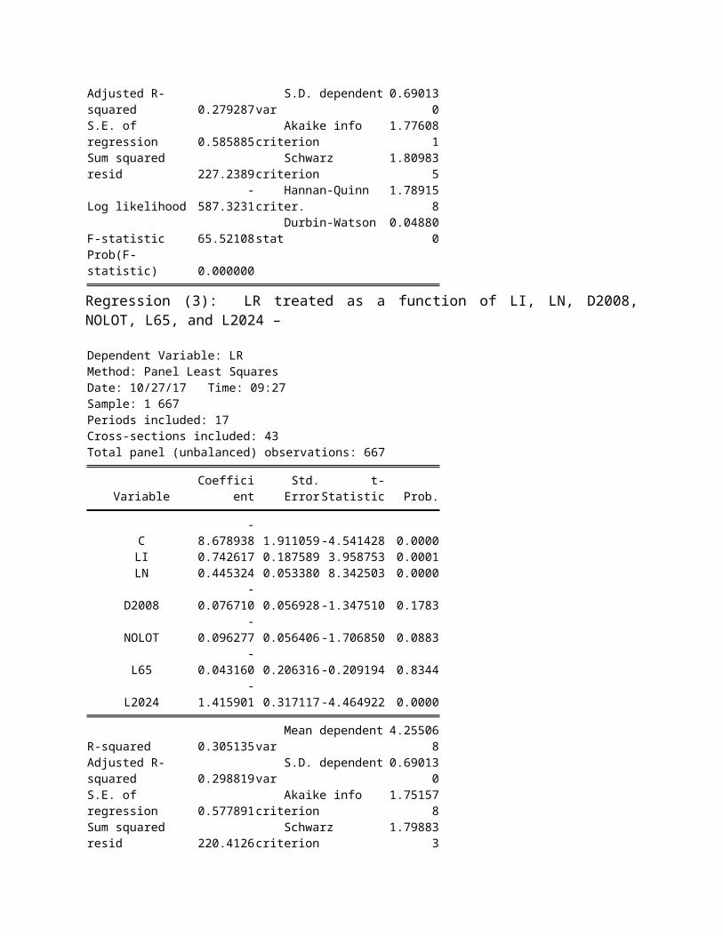
R-squared 0.283615    Mean dependent var 4.255068Adjusted R-squared 0.279287    S.D. dependent var 0.690130S.E. of regression 0.585885    Akaike info criterion 1.776081Sum squared resid 227.2389    Schwarz criterion 1.809835Log likelihood -587.3231    Hannan-Quinn criter. 1.789158

F-statistic 65.52108    Durbin-Watson stat 0.048800Prob(F-statistic) 0.000000

Regression (3): LR treated as a function of LI, LN, D2008, NOLOT, L65, and L2024 – Dependent Variable: LRMethod: Panel Least SquaresDate: 10/27/17 Time: 09:27Sample: 1 667Periods included: 17Cross-sections included: 43Total panel (unbalanced) observations: 667

Variable Coefficient Std. Error t-Statistic Prob.

C -8.678938 1.911059 -4.541428 0.0000LI 0.742617 0.187589 3.958753 0.0001LN 0.445324 0.053380 8.342503 0.0000

D2008 -0.076710 0.056928 -1.347510 0.1783NOLOT -0.096277 0.056406 -1.706850 0.0883

L65 -0.043160 0.206316 -0.209194 0.8344L2024 -1.415901 0.317117 -4.464922 0.0000

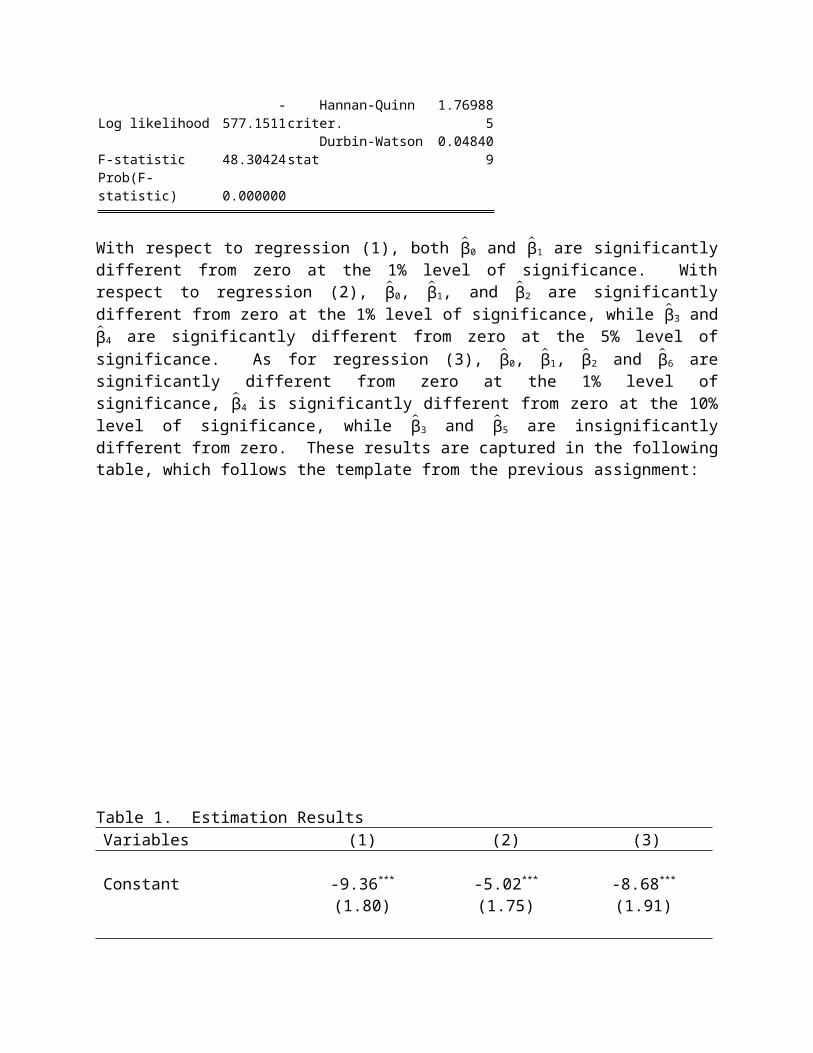
R-squared 0.305135    Mean dependent var 4.255068Adjusted R-squared 0.298819    S.D. dependent var 0.690130S.E. of regression 0.577891    Akaike info criterion 1.751578Sum squared resid 220.4126    Schwarz criterion 1.798833Log likelihood -577.1511    Hannan-Quinn criter. 1.769885F-statistic 48.30424    Durbin-Watson stat 0.048409Prob(F-statistic) 0.000000

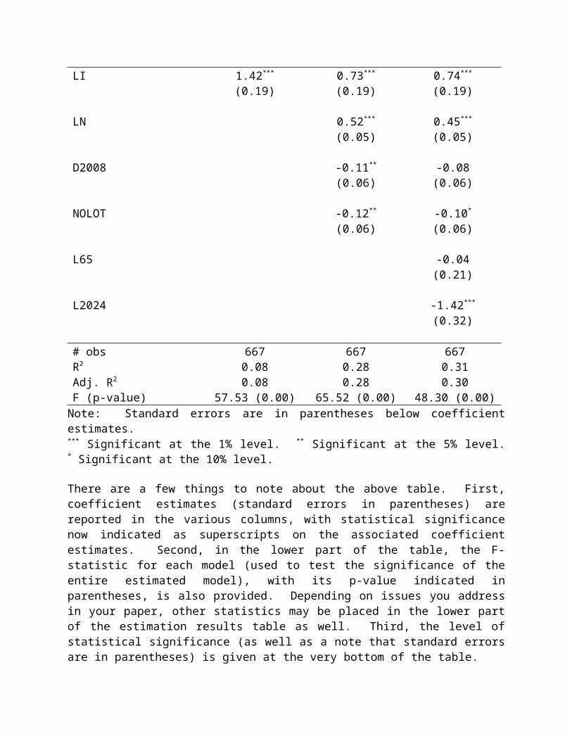
With respect to regression (1), both β̂0 and β̂1 are significantly different from zero at the 1% level of significance. With respect to regression (2), β̂0, β̂1, and β̂2 are significantly different from zero at the 1% level of significance, while β̂3 and β̂4 are significantly different from zero at the 5% level of significance. As for regression (3), β̂0, β̂1, β̂2 and β̂6 are significantly different from zero at the 1% level of significance, β̂4 is significantly different from zero at the 10% level of significance, while β̂3 and β̂5 are insignificantly different from zero. These results are captured in the following table, which follows the template from the previous assignment:

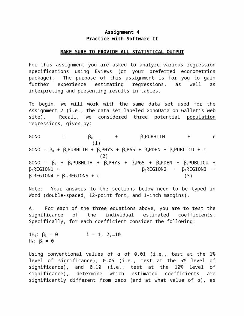
Table 1. Estimation ResultsVariables (1) (2) (3)

Constant

LI

LN

D2008

NOLOT

L65

L2024

-9.36***

(1.80)

1.42***

(0.19)

-5.02***

(1.75)

0.73***

(0.19)

0.52***

(0.05)

-0.11**

(0.06)

-0.12**

(0.06)

-8.68***

(1.91)

0.74***

(0.19)

0.45***

(0.05)

-0.08(0.06)

-0.10*

(0.06)

-0.04(0.21)

-1.42***

(0.32)

# obsR2

Adj. R2

F (p-value)

6670.080.08

57.53 (0.00)

6670.280.28

65.52 (0.00)

6670.310.30

48.30 (0.00)Note: Standard errors are in parentheses below coefficient estimates.*** Significant at the 1% level. ** Significant at the 5% level. * Significant at the 10% level. There are a few things to note about the above table. First, coefficient estimates (standard errors in parentheses) are reported in the various columns, with statistical significance now indicated as superscripts on the associated coefficient estimates. Second, in the lower part of the table, the F-statistic for each model (used to test the significance of the entire estimated model), with its p-value indicated in parentheses, is also provided. Depending on issues you address in your paper, other statistics may be placed in the lower part of the estimation results table as well. Third, the level of statistical significance (as well as a note that standard errors are in parentheses) is given at the very bottom of the table.

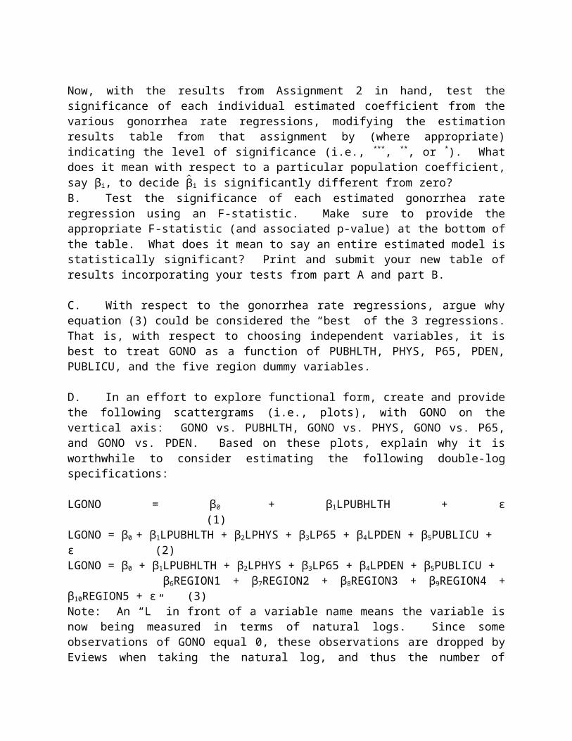
Now, with the results from Assignment 2 in hand, test the significance of each individual estimated coefficient from the various gonorrhea rate regressions, modifying the estimation results table from that assignment by (where appropriate) indicating the level of significance

(i.e., ***, **, or *). What does it mean with respect to a particular population coefficient, say βi, to decide β̂i is significantly different from zero? B. Test the significance of each estimated gonorrhea rate regression using an F-statistic. Make sure to provide the appropriate F-statistic (and associated p-value) at the bottom of the table. What does it mean to say an entire estimated model is statistically significant? Print and submit your new table of results incorporating your tests from part A and part B.

C. With respect to the gonorrhea rate regressions, argue why equation (3) could be considered the “best” of the 3 regressions. That is, with respect to choosing independent variables, it is best to treat GONO as a function of PUBHLTH, PHYS, P65, PDEN, PUBLICU, and the five region dummy variables.

D. In an effort to explore functional form, create and provide the following scattergrams (i.e., plots), with GONO on the vertical axis: GONO vs. PUBHLTH, GONO vs. PHYS, GONO vs. P65, and GONO vs. PDEN. Based on these plots, explain why it is worthwhile to consider estimating the following double-log specifications:

LGONO = β0 + β1LPUBHLTH + ε (1)LGONO = β0 + β1LPUBHLTH + β2LPHYS + β3LP65 + β4LPDEN + β5PUBLICU + ε (2)LGONO = β0 + β1LPUBHLTH + β2LPHYS + β3LP65 + β4LPDEN + β5PUBLICU + β6REGION1 + β7REGION2 + β8REGION3 + β9REGION4 + β10REGION5 + ε (3)

Note: An “L” in front of a variable name means the variable is now being measured in terms of natural logs. Since some observations of GONO equal 0, these observations are dropped by Eviews when taking the natural log, and thus the number of observations used to estimate these three equations is slightly lower than the linear versions estimated before.

Estimate each of the regressions corresponding to these 3 regressions above, providing your results in a new “estimation results” table (providing coefficient estimates, standard errors, R2, etc., etc.). In each column of this new table, be sure to indicate which coefficients are significantly different from zero (indicating at either the 1%, 5%, or 10% levels of significance). Also, test the significance of each respective model in its entirety by reporting F-statistics and associated p-values. That is, this new table should mimic the table you created in part B above.

Discuss the results. Is the elasticity of GONO with respect to PUBHLTH elastic or inelastic? E. Suppose you are interested in exploring whether or not the elasticity of GONO with respect to PUBHLTH differs across the 6 regions of California. To do this, modify equation (3) above and estimate the following:

LGONO = β0 + β1LPUBHLTH + β2LPHYS + β3LP65 + β4LPDEN + β5PUBLICU + β6REGION1 + β7REGION2 + β8REGION3 + β9REGION4 + β10REGION5 + β11REGION1∙LPUBHLTH + β12REGION2∙LPUBHLTH + β13REGION3∙LPUBHLTH + β14REGION4∙LPUBHLTH +

β15REGION5∙LPUBHLTH + ε

The elasticity of GONO with respect to PUBHLTH in each of regions 1 – 5 is then given by the following:Region 1: β1 + β11 Region 2: β1 + β12

Region 3: β1 + β13

Region 4: β1 + β14

Region 5: β1 + β15

Estimate the above equation and create a modified version of your estimation results using the following template:

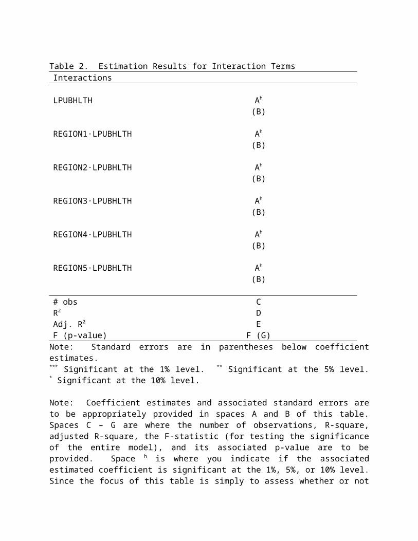
Table 2. Estimation Results for Interaction TermsInteractions

LPUBHLTH

REGION1∙LPUBHLTH

REGION2∙LPUBHLTH

REGION3∙LPUBHLTH

REGION4∙LPUBHLTH

REGION5∙LPUBHLTH

Ah

(B)

Ah

(B)

Ah

(B)

Ah

(B)

Ah

(B)

Ah

(B)

# obsR2

Adj. R2

F (p-value)

CDE

F (G)Note: Standard errors are in parentheses below coefficient estimates.*** Significant at the 1% level. ** Significant at the 5% level. * Significant at the 10% level.

Note: Coefficient estimates and associated standard errors are to be appropriately provided in spaces A and B of this table. Spaces C – G are where the number of observations, R-square, adjusted R-square, the F-statistic (for testing the significance of the entire model), and its associated p-value are to be provided. Space h is where you indicate if the associated estimated coefficient is significant at the 1%, 5%, or 10% level. Since the focus of this table is simply to assess whether or not this elasticity differs across regions, there is no need to report the results

associated with LPHYS, LP65, etc. (i.e., just report the coefficients, standard errors, etc. for the variables listed in the table above).

Comparing Region 6 to each of the other five regions, based solely on t-tests argue whether or not there are noticeable differences in the elasticity of GONO with respect to PUBHLTH. Which regions is Region 6 more or less similar to in terms of this elasticity? Explain.

Based solely on the estimated coefficients, calculate the estimated elasticity of GONO with respect to PUBHLTH in each of the six regions of California. In which region is the gonorrhea rate most responsive to county public health spending, and in which region is the gonorrhea rate least responsive to county public health spending? As a policymaker, how could such results be useful?

Assignment 5Preliminary Literature Summary and Reference List

For this assignment you will complete a preliminary version of your literature summary, as well as provide a preliminary list of studies cited. At this point, you are expected to have searched (using EconLit, Google Scholar, or some other search engine), read, and reasonably understood a minimum of 6 articles published in peer-reviewed Economics journals.

I. Literature Search

Obviously, before you summarize a literature, you have to identify some studies. To do this, you will need to do some sort of literature search. Regarding your search, consider:

The articles you choose should relate in some way to your research topic. For example, if you want to study the determinants of STD rates, such as you did in Assignments 2 and 4, then your articles should relate to this topic in some way. For instance, a reasonable paper to cite might be Chesson et al. (2000), entitled “Sex under the influence: The effect of alcohol policy on sexually transmitted disease rates in the United States”, which was published in the Journal of Law and Economics. An unreasonable paper to cite would likely be Waldfogel (1993), entitled “The deadweight loss of Christmas”, which was published in the American Economic Review. Waldfogel’s paper has nothing to do with STD, and thus is irrelevant to this topic.2

What makes a paper worthy of being cited? First, it could be the paper directly explores your issue in some way, such as the paper by Chesson et al. (2000) if your interest is in exploring STD rates. Second, it could be the paper explores a different issue from what you propose, but uses a similar empirical procedure you use in your analysis. For instance, Gallet and Doucouliagos (2014) use various methods to assess “publication selection bias” in the air travel demand literature. These same methods are used by Gallet and Doucouliagos (2017) to assess “publication selection bias” in the health outcomes literature. Although the topics are different, because the methods used are similar, the later study cites the earlier study. Third, a study of a topic different from yours, but using the same dataset, might be worth citing. For example, List and Lucking-Reiley (2002) use data collected from a field experiment in Florida, which is also used by List (2004). Thus, it is not surprising that the second paper cites the first paper.

Using either EconLit or Google Scholar, you can easily copy and paste the APA formatted citation of a study into Word. For example, in a Google Scholar search for

2 Regarding the citation of studies within the body of your paper, use the standard approach of author (year). For example, “Waldfogel (1993) finds…”. If there are two authors, list both author names. For example, “Saffer and Chaloupka (1999) find…”. If there are more than two authors, use et al. after the first author’s name. For example, “Chesson et al. (2000) find…”.

Chesson et al. (2000), you’ll see ” at the bottom of that particular listed study. Click on this and then you can copy and paste the APA formatted citation, which is:

Chesson, H., Harrison, P., & Kassler, W. J. (2000). Sex under the influence: The effect of alcohol policy on sexually transmitted disease rates in the United States. The Journal of Law and Economics, 43(1), 215-238.

You can then easily incorporate this into your reference list, making your writing go a lot quicker.

As you know, Economics is a highly-mathematical discipline. When reading papers, don’t get frustrated at trying to understand all the “mathematical gymnastics”. You’re an undergraduate major in Economics, and thus you are not expected to understand “differential equations”, “Lagrange multipliers”, “Hessian matrices”, etc. etc.

With this in mind, the best way to grasp the essence of a paper is to read its abstract and introduction (to get the “big picture” of what the study is addressing), read its literature summary (to see if there are other studies out there you might want to cite), glance at the statistical output (to identify the sign and significance of variables similarly used in your analysis), and then read the summary of its findings. Note whether or not the study finds results that are consistent with other studies or run counter to other studies.

It’s expected that you will search for studies, glance at them, and realize they are not worthy of your literature summary. Don’t simply search using EconLit or Google Scholar, pick off the first 6 studies listed, and then incorporate them somehow into your literature review. You need to read studies to see if they should be included or not.

II. Writing the Literature Summary

Regarding your literature summary, it needs to be at minimum 6 pages in length (double-spaced, 12-point font, and 1-inch margins). The last page will consist of your reference list. Consider the following:

The best way to begin writing a literature summary is to read. What I mean by that is in the papers you read you will notice how others structure their literature summaries. Mimic their style, but don’t plagiarize!

Don’t write your literature summary in the following way:

“The first study I read was by Chesson et al. (2012). They looked at…. Then I read Waldfogel (1993), who did…. The third paper I read was…”

A literature summary should be structured not according to the sequence in which you read papers, but rather by (i) how the literature has chronologically progressed or (ii) by themes within the literature, or (iii) perhaps some combination of (i) and (ii).

Some literature summaries will be chronological, in that they discuss the earliest work on an issue first, and then discuss key progressions in the literature over time. Other literature summaries will separate studies into various groupings, based on common themes. For instance, a literature summary might discuss how studies A, B, and C focus on issue D, while studies E, F, and G focus on a different issue, say issue H.

As suggested in Section I, your literature summary might include studies directly related to your topic, or indirectly related, via the use of similar empirical procedures or data.

Your literature summary should relate to the empirical model you propose to estimate. If in your empirical model you plan on assessing how X, Y, and Z affect W, then you should summarize studies that have examined issue W, as well as studies that have explored the roles played by X, Y, and Z.

For example, Gallet’s (2014) meta-analysis (which was provided to you) addresses the impacts of study characteristics on estimated price elasticities of demand for illicit drugs. In his empirical model, amongst other factors, he estimates how the price elasticity of demand is sensitive to (i) the type of drug being studied (i.e., marijuana, cocaine, and heroin), (ii) how quantity demanded is measured, and (iii) how price data is obtained. The literature summary is then built around these and other features of the literature. That is, effort is given to summarizing what the literature has found in terms of differences in price elasticities between marijuana, cocaine, and heroin, as well as differences in terms of how quantity is measured and how price data is collected.

Similar to Assignment 1, for the studies you summarize consider discussing such topics as: (i) the issue(s) addressed in the study, (ii) the data used in the study, (iii) the empirical model estimated in the study, and (iv) the key estimation results presented in the study.

In the final part of your literature summary you should discuss limitations of the literature and how your model addresses these limitations. Perhaps there are issues that the literature has not addressed thus far, or perhaps you propose to address similar issues as the literature but with different data or empirical techniques.

For example, Gallet (2017) mentions that several studies have examined how county-level spending on public health affects a variety of health outcomes, such as perceived health status and years of life lost. However, no study has addressed the impact of such spending on STD rates. The lack of literature in this area was one of the motivations for that study.

Bottom line, you have to argue that your model adds to the literature in some way and does not simply copy what others have done.

III. Reference List

The last page of this assignment will be a list of the papers you have cited thus far (with the word “REFERENCES” centered in bold at the top of the page). Following APA style, studies need to be listed in alphabetical order, based on the last name of the first author of the study. For multiple studies by the same author(s), the studies need to be listed chronologically. A study by a single author (e.g., List), who is a co-author of another study (e.g., List and Lucking-Reiley), needs to be listed first. Come see me to get more information on formatting if you like. You can also check out Nikolov (2013) for assistance. Based on the studies cited in this document, the reference list is given on the next page.3

3 Notice that Gallet and Doucouliagos have publications in 2014 and 2017. Rather than write their names twice, for the second study “_____” is used instead of their names. However, List has two publications, one on his own and one with Lucking-Reiley. Since the set of authors differs across these two studies, we do not use “_____” in the second study.

REFERENCES

Chesson, H., Harrison, P., & Kassler, W. J. (2000). Sex under the influence: The effect of alcohol policy on sexually transmitted disease rates in the United States. Journal of Law and Economics, 43(1), 215-238.

Gallet, C. A. (2014). Can price get the monkey off our back? A meta‐analysis of illicit drug demand. Health economics, 23(1), 55-68.

Gallet, C. A. (2017). The impact of public health spending on California STD rates. International Advances in Economic Research, 23(2), 149-159.

Gallet, C. A., & Doucouliagos, H. (2014). The income elasticity of air travel: A meta-analysis. Annals of Tourism Research, 49, 141-155.

_____. (2017). The impact of healthcare spending on health outcomes: A meta-regression analysis. Social Science & Medicine, 179, 9-17.

List, J. A. (2004). Young, selfish and male: Field evidence of social preferences. Economic Journal, 114(492), 121-149.

List, J. A., & Lucking-Reiley, D. (2002). The effects of seed money and refunds on charitable giving: Experimental evidence from a university capital campaign. Journal of Political Economy, 110(1), 215-233.

Nikolov, P. (2013). Writing Tips For Economics Research Papers.

Saffer, H., & Chaloupka, F. (1999). The demand for illicit drugs. Economic Inquiry, 37(3), 401-411.

Waldfogel, J. (1993). The deadweight loss of Christmas.  American Economic Review, 83(5), 1328-1336.

Assignment 6Preliminary Empirical Model and Data Summary

For this assignment you will provide a preliminary version of your empirical model and a summary of your data. It needs to be at minimum 5 pages in length (double-spaced, 12-point font, and 1-inch margins). There should be two sections to this assignment, say A and B. See each section below.

A. Empirical Model

In Section A, you are to present your empirical model. Specifically, you should discuss the dependent variable(s) and independent variable(s) of your model, as well as your testable hypotheses (i.e., how do you think the independent variables affect the dependent variable?). You should also discuss the theory which underlies your hypotheses.

For example, going back to Assignment 2, let’s say the focus is on the influence of county-level public health spending on the rate of gonorrhea. However, we also control for the influence of a variety of other factors on the gonorrhea rate. Accordingly, we propose the following relationship in the population:

GONO = β0 + β1PUBHLTH + β2PHYS + β3P65 + β4PDEN + β5PUBLICU + ε (1)

This is the preliminary model. You will need to define each of the variables corresponding to your version of equation (1), just as we did at the top of Assignment 2. Further, with respect to equation (1) above, how do you think each variable should affect GONO? For example, if we believe each of these variables has some influence on the rate of gonorrhea, then that corresponds to the coefficient of each variable not being zero in the population (i.e., β i ≠ 0 for i = 1, 2, 3, 4, 5).4 Accordingly, for equation (1) above, we will have 5 sets of testable hypotheses, given as:

HA: βi = 0HO: βi ≠ 0 for i = 1, 2, 3, 4, 5

Also, you will want to test the significance of the entire model. This corresponds to another set of null and alternative hypotheses, with respect to equation (1) above, given as:

HA: β1 = β2 = β3 = β4 = β5 = 0HO: at least one of the slope coefficients is not zero

Next, you will want to discuss alternative treatments of your model you plan to explore to see if the results are “robust”. At a minimum, you should mention you will explore how

4 You might want to go a step further and specify expected signs of the coefficients. However, in this case, you will be doing a one-sided t-test when testing a claim about a specific coefficient. If you like, come and see me for the proper technique to follow in this case.

sensitive results are to model specification. For example, with respect to equation (1) above, since the focus is on the role played by PUBHLTH, this could involve (i) seeing if the estimate of β1 (and its standard error) is sensitive to the omission or inclusion of combinations of other variables in the model (e.g., see equations (1) and (3) of Assignment 2) and (ii) seeing if the results are sensitive to functional form (e.g., recall the linear and double-log results in Assignments 2 and 4).5 Finally, although very specific to your model and data, you will need to mention other issues you plan to explore to check the robustness of your results. Issues such as multicollinearity, serial correlation (particularly if using time-series data), heteroscedasticity (particularly if using cross-section data), stationarity (if using time-series data), and the influence of fixed effects (if using panel data) may need to be addressed.

B. Data Summary

After discussing the empirical model in Section A, in Section B you will discuss your data. Specifically, now that you have defined the variables in Section A, you need to discuss the following:

What are the sources of your data? Is your data cross-sectional, time-series, or panel? What time periods and/or cross-sections does your data cover? What unit of observation are you working with (e.g., household, county-level, state-

level, etc.) and how many observations do you have? Are you missing any observations and/or did you drop any observations (and for what

reason(s))? Are you using any proxy variables?

It is worthwhile to have a table with variable names, definitions, and data sources provided. With respect to the gonorrhea rate regressions of Assignment 2, for example, a useful table is given on the next page.6, 7

5 Hint: Don’t simply try to replicate with your data what we did in Assignments 2 and 4. The issues you address will be different from what we did in those assignments, and thus will require you to think about what issues you should address in your model. Come and talk to me so that I can help you with your empirical model. 6 In the tables (and/or plots) you create in Assignments 6 and 7, place each one on a separate sheet at the end of the assignment. For example, in what follows I present two tables. These two tables should be placed on the last two pages of this assignment. At the end of the semester, all the tables you create will then be placed on the last few pages of your final paper. 7 Consider a few words of caution. It’s easy to go “overboard” with reporting lots and lots of descriptive stuff. Keep in mind this is not the most important part of your final paper. You don’t need to provide and discuss every conceivable descriptive statistic or plot. Try to keep it simple. Beyond basic descriptive statistics, such as the mean, standard deviation, etc., ask yourself if providing another statistic or plot adds sufficient value to your estimation results section to warrant discussing it.

Table 1. Variable Names, Definitions, and Data SourcesVariables Definition

Dependent Variable:GONO

Independent Variables:

PUBHLTH

PHYS

P65

PDEN

PUBLICU

REGION1

REGION2

REGION3

REGION4

REGION5

REGION6

Gonorrhea rate (i.e., number of cases per 100,000 population)

Real per capita spending on public health

Number of physicians per 1,000 population

Percent of the population age 65 and older

Population density (i.e., population per square mile)

= 1 if a CSU or UC campus is located in county i at time t, 0 if not

= 1 if county i is located in San Francisco Bay Region, 0 if not

= 1 if county i is located in Southern California (excluding LA) Region, 0 if not

= 1 if county i is located in Los Angeles Region, 0 if not

= 1 if county i is located in Central/Southern Farm Region, 0 if not

= 1 if county i is located in North/Mountain Region, 0 if not

= 1 if county i is located in Central Valley Region, 0 if not

Note: Data on GONO came from the California Department of Public Health (http://www.cdph.ca.gov), while data on PUBHLTH came from the California State Controller’s Office (http://www.sco.ca.gov/index.html). Data on PHYS and PDEN came from Rand California (http://ca.rand.org/stats/statistics.html), while data on P65 came from CDC Wonder (http://wonder.cdc.gov/). Region designations were based on a report from the California Department of Social Services (2002). PUBLICU, REGION1, REGION2, REGION3, REGION4, REGION5, and REGION6 were constructed by the author.

Note: Now that you provide data sources, you will need to appropriately include them in the reference list you created in the last assignment.

Next, you need to provide and discuss descriptive statistics. At a minimum, you need to provide a table with the mean, standard deviation, minimum, and maximum values of each variable. For instance, with respect to Assignment 2, recall we created the table provided on the next page.

Table 2. Descriptive Statistics

Variables MeanStandardDeviation Minimum Maximum

Dependent Variable:GONO

Independent Variables:

PUBHLTH

PHYS

P65

PDEN

PUBLICU

REGION1

REGION2

REGION3

REGION4

REGION5

REGION6

40.77

61.76

1.99

13.24

365.32

0.39

0.17

0.11

0.02

0.22

0.37

0.12

36.89

33.27

1.04

3.69

695.92

0.49

0.37

0.31

0.13

0.42

0.48

0.32

0

2.96

0.30

6.48

1.70

0

0

0

0

0

0

0

166.20

174.91

6.20

23.30

3910.80

1

1

1

1

1

1

1

Depending on your topic, it will be worthwhile to refer to your descriptive statistics table and discuss some features of your data. For example, with respect to the above table, while the mean gonorrhea rate is roughly 41, a few less-populated counties (e.g., Colusa, Del Norte, Modoc, Mono, and Trinity) periodically reported no cases of gonorrhea. The maximum rate of roughly 166 was reported in Fresno County in 2006. Further, the lowest (highest) per capita spending on public health was observed in Stanislaus (Inyo) County, while Region 5 (3) has the greatest (least) share of counties.

Depending on your issue, you might also want to provide some plots of your data. For example, if you’re working with time-series data, plotting your variables over time would be useful to show the reader any trends in observations. You might also consider creating a table of correlations or creating scattergrams to illustrate preliminary relationships between variables. But, again, consider footnote 7.

Assignment 7Preliminary Estimation Results

For this assignment you will provide a preliminary discussion of your estimation results. It needs to be at minimum 5 pages in length (double-spaced, 12-point font, and 1-inch margins).8 Use the table template from Assignment 4 to construct your table(s) of estimation results. You should discuss the following:9

Do the coefficient estimates make sense? That is, do they support your expectations from Assignment 6? Do they support some theory? How do they compare with other studies in the literature?

Do your models explain much of the variation in your dependent variable (i.e., discuss R2 and/or adjusted R2)?

Which coefficient estimates are significantly different from zero (i.e., t-test results)? What can we then say about relationships in the population?

Are the estimated models significant (i.e., F-test results)? Are your results robust to alternative specifications? Are your regressions sensitive to other issues, such as serial correlation,

heteroscedasticity, and multicollinearity? If so, what happened to the results when you corrected for these issues?

Are there any results that surprise you? What might be plausible reasons for such results?

Assignment 88 Before reporting results, there are a few things to consider. First, you don’t have to estimate endless different regressions and report endless numbers of results. Estimate your initial proposed regression from Assignment 6, and then consider a few alternatives to address specification issues. Second, it’s not pleasing to the reader to decipher unusually small or large values. Try to report results only to a few decimal places. In the event that your coefficient estimates are very small or very large, you might want to change some units of measurement. For example, let’s say you include per capita income as a regressor (measured in dollars), obtaining an estimated coefficient of 0.00001. Rather than report such a small value, you could re-scale income to thousands of dollars, and by doing so obtain an estimated coefficient of 0.01.9 Similar to Assignment 6, place each table you create on a separate sheet at the end of the document you create. These tables will then be placed at the end when you assemble your final paper.

Preliminary Introduction, Conclusion, and Title Page

For this assignment you will provide preliminary versions of your introduction, conclusion, and title page. The introduction (1 page minimum) and conclusion (1.5 page minimum) should be relatively short, no more than 3.5 pages total. The title page will be 1 page in length. Similar to all other assignments, your document must be double-spaced, 12-point font, and 1-inch margins.

I. Introduction

In this section you “welcome” the reader to your paper. As such, it is important to grab the reader’s interest. Begin by mentioning the topic that you are studying and explain why it is an important topic. Do not cite too much literature in this section, as that is the purpose of your literature summary. Depending on your topic, though, you might cite a statistic or two that helps “sell” the importance of your topic.

It is important in this section to mention what your main contribution is to the literature. That is, you might say something like “While much of the literature has addressed the impact of X on Y using approach Z, my paper is unique in that it considers….”.

Towards the end of this section you should briefly mention the key results of your study (perhaps a paragraph). Then in the last sentence of the introduction say something to the effect that “the remaining sections of the paper provide a literature summary, empirical model and data summary, and estimation results. The paper concludes with a summary of the findings and recommendations for further analysis.”

II. Conclusion

In this section you should begin by mentioning the topic that you addressed and the key results of your analysis (perhaps a paragraph or two). You might also mention how your results are useful. For example, if your results have policy implications, it would be worthwhile mentioning them here, which could easily fill a paragraph or two.

Near the end of the conclusion you should mention limitations of your study (e.g., perhaps data was lacking to address an important issue, etc.), as well as suggestions for future research to consider.

III. Title Page

On the title page (see sample paper I provided) you need to first provide the title of your paper, then your name, your affiliation (i.e., California State University at Sacramento), and then May 2018 (i.e., the month you submit your paper). Then provide a maximum 150 word abstract.

The abstract is meant to be a very short statement covering the main points of your paper. You should briefly mention the key findings and how these compare to the literature in general.

IV. References

Now that you have the preliminary versions of each section of your paper complete, make sure to also provide a final list of references with this assignment.