CHAPTER SEVEN

PRECESSIONAL THEORY

ECE2 theory gives an exact description of light deflection due to gravity and also of

planar orbital precession, as described in UFT342 and UFT325, where a fundamental new

hypothesis was introduced, one that imposed an upper bound on the Lorentz factor. It was

shown in UFT325 that massive particles such as electrons can travel at the speed of light

without violating fundamental laws. This fact is well known experimentally at accelerators

such as SLAC and CERN, which routinely accelerate electrons to c. The new hypothesis of

UFT325 also means that photons with mass can travel at c. In UFT328 planar orbital

precession was described without additional hypothesis simply by simultaneously solving the

hamiltonian and lagrangian ofECE2 theory. None of these methods use the incorrect and

obsolete Einstein theory.

The planetary precession of the perihelion is known experimentally with claimed

accuracy, although there have been severe criticisms by Myles Mathis and others, developed

in the UFT papers on www.aias.us {1- 12}. Accepting the experimental claims for the sake

of argument, the experimental data are summarized empirically as follows:

( -;_ d.. .. - - ( 'J \ t E- (oS (;r8)

~ ,jM.(r -7(

c'lr£ in plane polar coordinates ( r, e ). Here M is the mass of an object around which an

object m orbits. G is Newton's constant, cis the universal constant known as the vacuum

speed of light and rL is the half right latitu~e of the orbit, for example a precessing

ellipse and f is the eccentricity. Both J and t are observable with precision. In

the solar system x is very close to unity.

As in previous chapters the ECE2 lagrangian is:

J LC H ---Y\o\ c.,.. -. -~

and the ECE2 hamiltonian is:

') t-li ~ - O~v -

in which the Lorentz factor is: - t/J.

Note carefully that v _tJ

is the Newtonian velocity. The experimentally observable

velocity is always the relativistic velocity:

--In these equations U is the potential energy of attraction between m and M. The Euler

Lagrange analysis ofUFT325 and UFT328 defines the relativistic angular momentum: "') .

l -:=. \{ V',_( 8 - c-,) which is a constant of motion:

The Newtonian and non precessing planar orbit is:

' __1-- - ( ") \-\- ~c~>se

and is described by the non relativistic hamiltonian:

and non relativistic lagrangian:

In this case the non relativistic angular momentum:

., e· \_ () ':.. ~{ 0

is the constant of motion:

0.

The relativistic angular velocity is

and the non relativistic angular velocity is:

CJo

The relativistic orbital velocity is defined as follows in terms ofthe relativistic

angular momentum: ) (Jvf ) < -\- -JJ

From Eqs. ( i_. ) and ( \L ):

- ,L - )

<

Eq. ( b ) means that:

From Eq. ( ~ ):

--

It follows from Eqs. ( \~ ), ( \(

J L

1 ,L 1- 0.

1 -----")--< ~

an equation which is analyzed numerically and graphically later in this chapter. It is

demonstrated that r l6) from Eq. ( )J! ) is a precessing ellipse. This confirms the results

ofUFT328 and shows that ECE2 relativity produces a precessing ellipse directly from the

lagrangian and hamiltonian, without any additional assumption. This theory is Lorentz

covariant in a space of finite torsion and curvature and is part of the ECE2 generally

covariant unified field theory.

In UFT343 the Thomas and de Sitter precessions are developed with ECE2

relativity. In the standard physics, Thomas precession is the rotation of the Minkowski line

element and de Sitter precession is the rotation ofthe Schwarzschild line element. In previous

UFT papers { 1 - 12} it has been shown that the derivation of the Schwarzschild li.ne element

is riddled with errors, notably it is based on an incorrect geometry without torsion. The

Thomas frame rotation in the Newtonian limit is:

where (,.) e is the constant angular velocity of frame rotation. The angle e t is that of

a rotating plane polar coordinate system denoted ( r' e I ). The total angular velocity is

defined by:

GJ -\ -

and the classical lagrangian is:

where:

The Euler Lagrange equations are:

d~L - . c)Q. \

and

Ji, Z)c

--

-

-(u)

)f. (:J-5) ~ ]I~~'

- CJ0 JJ, ~ - .. Jl ~(

from which the conserved angular momentum in the rotating frame is: '") ") L, -=- Y\-.( {._9, ... L + W 13 fh-(

-(:n)

where:

Jl

L -=- V)..() M - (l~ Ji

is the conserved angular momentum of the static frame ( r, e ). Both L and L \

constants of motion.

are

where:

is the gravitational potential. As shown in Note 343(2) the hamiltonian produces the rotating

conic section:

(n which the time is defined by:

-Eqs. ( ~ \ ) and ( 3>l ) can be solved simultaneously by computer algebra to giver in

terms of e _,

-:... Cos ~\

\ -

an equation that can be inverted numerically to give a plot of r against theta, the required

orbit.

The orbit of de Sitter precession follows immediately as:

where it is known experimentally that:

)( -

The halfright latitude ofthe rotating frame is: ( [\

I .~ L;· - ~~ ~\ -~m.(s.·

\'\... -and the eccentricity in the rotating frame is: )

1_ + )_H_, L_, -----=­~ ~ WL") & ., ~-

f,

The reason for Eq. ( ~'--\- ) is that de Sitter or geodedic precession is defined by rotating the

plane polar coordinates system in which the precession of the planar orbit is observed. The

original method by Sitter was much mor complicated and based on the incorrect Einstein

field equation.

In contrast, Eq. ( ~~ ) is rigorously correct and much simpler, and based on the

theory ofECE2 relativity.

The orbital velocity from Eq. ( 3 \ ) is:

~ L~

in which the relativistic velocity is:

The relativistic velocity is the one defined by Eq. ( 3 ~ ):

~~ ~ ~~ ( It follows that:

l -l -

in which both L and L I are constants of motion. Here 8 I is defined by:

~I "" e -\- Wll t. ~ ( 4-:)

--

~ _ ( ~~~)"l 7"} + ~·, s•~ 1 and the Thomas angular velocity (the relativistic angular velocity) is: \ ·

SL-\ -C~Lt) This was used in UFTll 0 to define the Thomas phase shift.

In the numerical analysis and graphics ofUFT343 it is shown that the Thomas

precession produces a precessing orbit, which is therefore produced by rotating the plane

polar coordinate system.

Planetary precession can also be thought of as a Larmor precession as described in

UFT344, it is the Larmor precession produced by the torque between the gravitomagnetic

field of the sun and the gravitomagnetic dipole moment ofthe planet. In general any

astronomical precession can be be explained with the ECE2 gravitational field equations.

This goes beyond what the obsolete Einstein theory was capable of. In UFT318 the ECE2

gravitational field equations were derived in a space in which equation are Lorentz covariant,

and in which the torsion and vurvatire are both non zero. This is known as -ECE2 covariance.

In UFT117 and UFT119 the gravitomagnetic Amp~re la~ was used to describe the earth's

gravitomagnetic precession and the {ecession of the equinox.

Consider the magnetic dipole moment of electromagnetism:

-where -e is the charge on the electron, m its mass and L its orbital angular momentum. The -following torque:

\'\f ---

is produced between m and a magnetic flux density B. Such a torque is animated by the well - -known Evans Pelkie animation on www.aias.us and youtube. The Larmor pecessional

frequency due to the torque is:

-=-- ~o t ~

d..~ where g is the Land{ factor described in previous chapters.

This well known theory can be adapted for planetary precession by calculating the

gravitomagnetic dipole moment and using the orbital angular momentum of a planet. The

charge-e on the electron is replaced by the orbiting mass m, so the gravitomagnetic dipole

moment is:

L - -L l -(4-<i\ l- :J

and is a constant of motion. The orbital angular momentum is defined by:

L .~ { )'.." ' - --- -

where vis the orbital velocity of m and where r is the distance between m and M. Therefore:

In general this theory is valid for any type of orbit, but for a planar orbit:

L = V\-< --r { ( ~0 -A torque is formed between.:<>;) amd the gravitomagnetic field ~ ofECE2

general relativity:

'~ ------ _(s~

resulting in the gravitomagnetic Larmor precession frequency:

I where O '( is the gravitomagnetic Lande factor. The precession frequency of a planet in

this theory is the gravitomagnetic Larmor precession frequency. For example consider the

sun to be a rotating sphere. It rotates every 27 days or so around an axis tilted to the axis of

rotation of the earth, so h {c:vett is not parallel to k $""'"'- and there is a non

zero torque. The gravitomagnetic field ofthis rotating sphere in the dipole approximation is:

Q --s~

--

~

Here r is the distance from the sun to the earth. The rotation axis of the sun is tilted by 7.25

to the axis of the earth's orbit, so to a good approximation:

L s~ · ' -D - (ssj

and in this approximation:

--s~

The torque is therefore:

and is non zero if and only if1:.~~ and\,.~'\!. are not parallel, where ~"'It is the

angular momentum of the earth's spin and ks~ is that of the sun's spin. The angle

sub tended by l and b is approximately 7.25 °. -.q~ s"-The magnitude of the angular momentum of the sun can be modelled in the first

approximation by that of a spinning sphere:

:l --- s where I is the moment of inertia and R the radius ofthe sun. Therefore the magnitude of the -

'fY\ fs ~ .. ......,.,..

gravitomagnetic field of the sun is:

s c.."') (<.

where G.:> is its angular velocity. After a rotation of :l.1r radians:

where Tis about 27 days. Therefore:

.L where:

and where the radius ofthe sun is: C,

Q -::. 6 . '\ S l ')(. \o

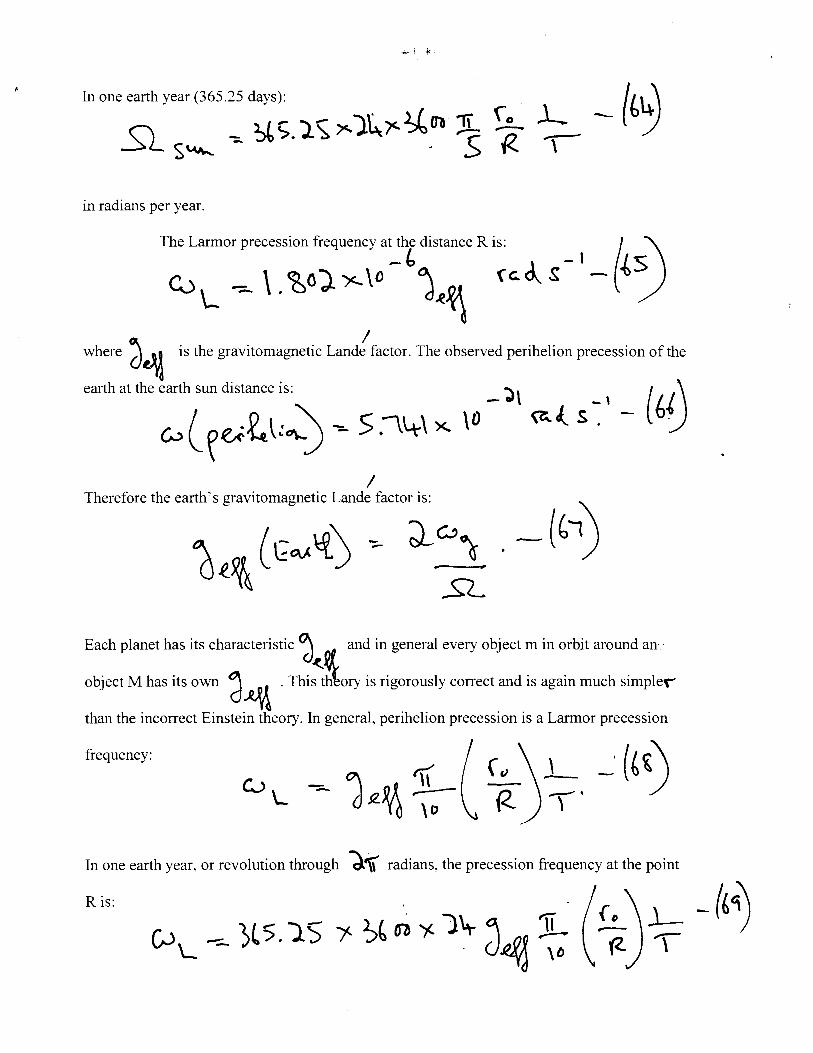
In one earth year (365.25 days):

n -==- ~ S. l ~ :><-)~ :><-~ 01 :!L ~L s~ · S

in radians per year.

J.._

\

- b .1 -' ~s The Larmor precession frequency at the distance R is: (. 0 C0 L _,_ \. ~ o). ')<.. \ o j .(~ {c. <:>... & -

I where d~ is the gravitomagnetic Lande factor. The observed perihelion precession of the

earth at the earth sun distance is: _ } I _ 1

(

1\

w ( ~~t \:~ ""- s .\4-\ X. \0 (?;. .{_ s . 6~ I

Therefore the earth's gravitomagnetic Lande factor is:

Each planet has its characteristic j.(_pJ_ and in general every object min orbit around an

object M has its own j~ . This fu{ory is rigorously correct and is again much simpler

than the incon-ect Einstein theory. In general, perihelion precession is a Larmor precession

frequency:

' -----. ' In one earth year, or revolution through ~'\\ radians, the precession frequency at the point

R is:

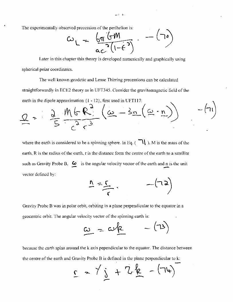
The experimentally observed precession of the perihelion is:

CJL -- ~~rrr·&M . - (,'";\ "':\ \ -E- ")) /

C\.v Later in this chapter this theory is developed numerically and graphically using

spherical polar coordinates.

The well known geodetic and Lense Thirring precessions can be calculated

straightforwardly in ECE2 theory as in UFT345. Consider the gravitomagnetic field of the

earth in the dipole approximation { 1 - 12}, first used in UFT 11 7:

Q ~. ~ ~~~~ (~-s~(~·~)) -- c . ':). . ~

....? -(__ ·C

where the earth is considered to be a spinning sphere. In Eq. ( \\ ), M is the mass ofthe

earth, R is the radius of the earth, r is the distance form the centre ofthe earth to a satellite

such as Gravity Probe B, W - is the angular velocity vector of the earth and n is the unit -vector defined by:

f\ -::::.. \ - _.. ' .----(

Gravity Probe B was in polar orbit, orbiting in a plane perpendicular to the equator in a

geocentric orbit. The angular velocity vector of the spinning earth is:

CJ -- -because the earth spins around the k axis pependicular to the equator. The distance between

the centre of the earth and Gravity Probe B is defined in the plane perpendicular to k:

-

so:

(\- ~~: i -?'~ i .- (t~ < '(

b The experimental inclination of Gravity Probe B was almost exactly 90 .

Therefore in the dipole approximation, as in UFT117:

") ' -~i.) ~ -~Yz ~ Q ~ Yf\&~ ~

---------; ') ") -s c.-'") < "( '<

-r-ij

The Gravity Probe B spacecraft carried precision gyroscopes which are currents of massand

which are therefore gravitomagnetic dipole moments ( rh ). The torque between the earth -and the spacecraft is:

---

This is known in the standard literature as Lense Thirring precession .. The relevant data are

as follows:

At the equator:

":>lt {p,._ M --=-. s. q ~ ~ \Ob 0

(2. -=. b . t>l ')<.. \ 0 b "" ~ _ 1 .o :l )(. \o ~~ _, c - :l. ~ <\ <6 '>< \~ \\ ~ s- l - ')

~ -=- {,. bf )<.. \O 6 .s s. .J -I

w -=--I . :l.<\.).."' \ o - ~{;\. S

- -

-1 !<

and the magnitud f h . eo t e gravitomagnetic field ofthe earth fro E ( _.,b . • m q. \ ) IS:

.Jl -=. \ • ~ ~ )<.. \0 --1\.,. ~.!..._ S- I - (~ ~

expenmental value from UFT117 of: compared with the · .. s~.t~V ..,_ \ . 'lb><- 1 o- '4-~ s ~ ' - ( ~:0 More generally: ~· ~ ~ ~wi -(<{V and:

1 ~l~· ~) ~ ~ 7,~ '(

It follows that:

"\-

~i,_ ~ -;:_ 1t (•fe -=- 1 -{~) 0 ---I -< <

Defining:

then: ~ _:>~ ( ~. ~) ~w (~3s•:: e !__ -~s,·~.-8 r6sB i . -(0 Therefore the Lense Th. . . . Irnng precessiOn Is:

_Q_LI ~ ~~~.,~J -[ (\-)s~~e)! ->si~.Br·sBj_ \. Later in this chapter an average value of the precession is worked out and the - ( ~l

latitude identified for precise agreement with Gravity Probe B. In general the Lense Thirring

precession depends on latitude, so it is assumed that the experimental result is an average. It

is not clear from the literature how the Lense Thirring effect is isolated experimentally from

the geodetic precession. For the sake of argument we accept the experimental claims.

where r 0 is the magnetic permeability in vacuo. In Eq. ( g q ) m is the magnetic -dipole moment:

---The gravitomagnetic vacuum permeability ofthe ECE2 field equations is:

u. .,__ 4u (, - C "0 / 0 (,.. "1. ')

G-

so:

where the gravitomagnetic dipole moment ~ ~ is defined in analogy to Eq. (

Yh -=- l- L ( q~ -c )... -· ~

qo )by

The angular momentum of the spinning spherical earth is:

L --so:

--

The geodetic precession is is calculated from the same starting equation as the

Lense Thirring precession:

'IV\& ~ ......

:lc? ( The vector \is defined by Eq. ( \ '-T ) because Gravity Probe B was in polar orbit once

every 90 minutes, giving an angular velocity of:

c., -=-

As seen from a frame of reference fixed on Gravity Probe B, the earth rotates at a given

angular velocity, generating the angular momentum:

--for an assumed circular orbit, a good approximation to the orbit of Gravity Probe B. If it is

assumed that:

-perpendicular to the polar orbit, then:

For the earth:

If it is assumed that r is the distance from the centre of the earth to Gravity Probe B then:

. b ( . ( -:::._ \. ol )(_ \o ~ - \bJ.)

-1 !<

g1vmg:

The experimental claim is:

5L l .a::ci) - \ . 0 lb )<... \0

The theory is in good agreement with the experimental claim. It has been assumed

that the angular momentum needed for Eq. ( OU, ) is generated by a static earth in a

rotating frame. This is the passive rotation equivalent to the active rotation of Gravity Probe

B around the centre of the earth in a polar orbit once every ninety minutes. Exact agreement

I with the experimental data can be obtained by assuming an effective gravitomagnetic Lande

factor, or by assuming that the rotation is described more generally by:

--- -and

( -Later on in this chapter, computer algebra and graphics are used to evaluate the magnitude:

x-=- \ ~- ~~(~ • ~)\ -(lol) from Eqs. ( \0 S ) and ( \ () ~ ). Therefore exact agreement with Gravity Probe B can

be obtained from the gravitational field equations of ECE2.

These field equations can be used to explain any astronomical precession in terms

of magnitude of vorticity and the result can be expressed in terms of the tetrad and spin

connection of Cartan geometry. This theory can be applied to the Lense Thirring, geodetic

and perihelion precessions to give exact agreement in each case in terms of the vorticity of

the underlying mathematical space of the ECE2 theory. Th~ perihelion precession in this

type of theory is developed in terms of the orbital angular momentum of the sun as seen from

the earth. In general any precession can be developed in terms of the magnitude of the

vorticity spacetime, which can be expressed in terms of a well defined combination of tetrad

and spin connection. This combination appears in the ECE2 gravitational field equations.

As shown in Notes 346(1) to 346(3) any precession can be described in the dipole

approximation in terms of angular momentum L:

( L

When this equation is applied to perihelion precession of the earth about the sun, r is the -distance from the earth to the sun. If the sun is considered to rotate about an axis k, the plane -tl of the earth's orbit is inclined to the plane perpendicular to k at an angle of 7.25 . So as in

Note 346(3):

The observed precession ofthe earth's perihelion is: _ \$. «} _ \ (\\~

.s:L_ .,_ ( o .o~ !._ o. o\:l.)'' "'- 'j~ -=-I .b ~\ ><- \o c s. - )

From the emth, the sun appears to be orbiting with an angular momentum:

where M is the mass of the sun, and where ~ is the angular frequency of the orbit. The - .., earth rotates around the sun once every year, or P. \5, ~ \0 XC, so:

~J__ ~- ~ -(\\d) - -, 3. \~'><. \0

--

Using:

the perihelion precession is found to be:

. - 'S -' SL -=. 0 . q_ X\ ~ \0 . ~<l s. .

Exact agreement can be found by using an effective angular momentum L The above theory -~

has used a circular orbit in the first approximation.

The fundamental assumption is that the orbit of the earth about the sun produces a

torque:

where ~";) is the gravitomagnetic dipole moment:}_ l

fl\6 ~-and where is the gravitomagnetic field. Here L is the orbital angular momentum. -The gravitomagnetic field is the curl of the gravitomagnetic vector potential:

..Q - "'! '!'-.. ~~ -(\\~ - ,---- - '

so: & \_ ')<.. ( -(\;},_0 w -:::.... -· --) ;) "') _!,

(._..(

In direct analogy, the Lense Thirring precession of the earth with respect to the sun is due to

to the latter's spin angular momentum about its own axis. !he sun spins once every 27 days

about its axis, so the relevant angular momentum in this case is the spin angular momentum

ofthe sun:

--L -~

Similarly the Lense Thirring precession of Gravity Probe B is due to the spin of the earth

every 24 hours. This spin produces a mass current and a gravitomagnetic dipole moment:

~d ur0 ~ ~_s _(\:D.) due to spin angular momentum.

The perihelion precession of the earth is a geodetic precession caused by an

orbital angular momentum, the orbital angular momentum of the sun, which is observed in ·a

frame of reference fixed on the earth.

As in previous chapters the magnetic flux density B of ECE2 theory can be -defined by curvature through theW potential: -

--- -The ~_potential is defined by torsion, and S-.S is the spin connection vector. In precise

where:

and where J:"Q is the scalar potential of gravitation. Note that ~j has the units of

linear velocity, so:

---

which defines the gravitomagnetic field as a vorticity in analogy with fluid dynamics. This

analogy is developed later in this book in chapters eight and nine. The vorticity is that of

spacetime, or the aether or vacuum.

It follows that any precession can be defined precisely as follows:

52_ ~ ~ \ _g \ ~ ~ \ 'i~ ~~\-(\d) so all precessions of the universe are due to the vorticities of ECE2 spacetime, vacuum or

aether. If it is assumed that:

0

then the spacetime is inviscid, and in chapters 8 and 9 it is shown that spacetime is in general

a fluid. The field equations of fluid dynamics can be unified with those of electrodynamics

and gravitation.

The equations of gravitomagnetostatics are:

'I ~.2. - Y\ ')(.. ~ -- ~ ~ ~· 2~ - (\l") (._..

where:

---Here) is the current density of mass, q is the tetrad vector. ~ .S is the spin connection

-Y\o-. (o) -vector, and where ( is a scalar with units of metres. It follows from Eq. ( \~~)that

~ . 'J '-,(.. _SL - '4 . \;( )<.. ..S2. -:- 0 . - ( H'0 - -- --Now use:

"'3_·('1-~~J - ~. ( ~ ')(-~)- \((· l '}_ --~-~) - --{\!>)) - 0 -

so:

One possible solution is:

- ~ \(( - ~--where:

Therefore the ECE2 equation of any precession is:

where:

These are generally valid equations without any approximation, and are based on Cartan

geometry.

In the dipole approximation:

_Q_ -:-~ 'l_ ~ - ~c]

and comparing Eqs. ( \?t ) and ( \b ~ ):

~ -=- ~ • L ~.£ . - ( t~~ --o ~z(b

This is also an expression for theW potential. Finally: ~

~-=-~·'i-,c.c~~~ ~/'!-~(~~) ~c, ~) .(

_( \'+o\

which shows that any precession is due to Cartan geometry, Q.E.D . . Later in this chapter a numerical analysis w_ith graphics is given using computer

algebra to check the above calculations.

Using ECE2 relativity and the minimal prescription the hamiltonian for a particle

in the presence of a gravitomagnetic potential can be defined. The lagrangian can be

calculated from the hamiltonian using the canonical momentum and the relevant Euler

Lagrange equations used to derive the gravitomagnetic Lorentz force equation. In the absence

of gravitomagnetism this equation reduces to the Newton equation. The precession frequency

of the Lorentz force equation is an rbital precession frequency of any kind. This method

gives a simple general theory of precession in ECE2 relativity.

Consider the gravitomagnetic minimal prescription:

in which the linear momentum of a particle of mass m is incremented by the gravitomagnetic

vector potential:

The free particle hamiltonian becomes: '") "') L jL

\~ ~ L (~ \-V\-.'Ld'j·(f \-~~\-:-.+-+-I~'\[) ti-· -" ~n... - - ) d."' - (l~\

where the orbital angular momentum is: ,..... )

-(\~ l --- -and the gravitomagnetic field is the vorticity:

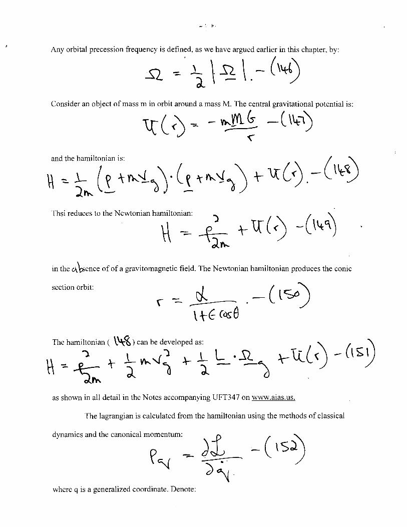
Any orbital precession frequency is defined, as we have argued earlier in this chapter, by:

Q \ \ ~ \ . - ( \~) Consider an object of mass min orbit around a mass M. The central gravitational potential is:

~r<L (:. -C \4,1)

in the V\ \,;ence of of a gravitomagnetic field. The Newtonian hamiltonian produces the conic

section orbit:

d._ .. -(lSP) \ tf (ose

The hamiltonian ( \~<6) can be developed as: _ ) ( _ 9 "') \ ~1 '- J_ L ._st -t-lll< - l~\

~ -=-~ t- - V\o.. ) .,.- 'l - -~ ~~ ~ 0 '

as shown in all detail in the Notes accompanying UFT347 on \Vww.aias.us.

The lagrangian is calculated from the hamiltonian using the methods of classical

dynamics and the canonical momentum:

where q is a generalized coordinate. Denote:

then:

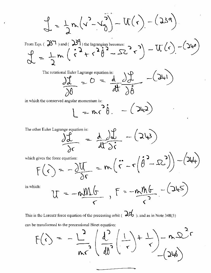
-The lagrangian is therefore:

In general:

and

'l-"'-~ ~ !L. - - c\~~ So:

~! =-~\l(<)-~ ((~. ~J~d T~ ~(~x 'idV . The right hand side ofEq. ( \$')is: - ( \~ 1.')

c\ r )'1 ,_ ~ (vr-.( - 11\o.._ '{"'\ - (\'~ 1[~~ JS - o) / -

Now define:

and:

to find the gravitomagnetic Lorentz force equation:

~ ~- - - Jr._ ( s) f -where:

--

is the gravitomagnetic analogue of the acceleration due to gravity in ECE2 relativity.

The precession of any orbit is therefore governed by the gravitomagnetic force law

( \'\ \ ) with precession frequency ( \~).

From Eqs. ( \t~) and ( \~l ):

r~ .,. and it follows that:

--

so:

"'l

<

The gravitomagnetic Lorentz force is therefore:

.e.

") (

_,

-(t'fj - -n-.m&-- ~<"+"' ~~d < ') JI

••

-- -

where: \ ---

In the absence of a gravitomagnetic field Eq. ( \1b) reduces to the Newtonian:

-~m~ .:t., -(n~ -••

-- < For a planar orbit it is well known that: •

• --

in the absence of a gravitomagnetic field. The acceleration in the absence of a

~ !_ ( r i_, ~ (8 .i-e) Jr -(t"'o)

gravitomagnetic field is: •• ( -- -

an expression which gives rise to the well known centrifugal and Coriolis forces. So the

gravitomagnetic force terms occur in addition to these well known forces, and result in

precession, whereas the centrifugal and Coriolis terms do not result in a precessing orbit as is

well known.

The gravitomagnetic field is governed by the gravitational equivalent of the -' Ampere Law { 1 - 12}:

- - - .S:11 ~> ~d -(\<6~ ·c...-

where ~~is the localized current densi~ of mass, analogous to electric current density in

electrodynamics. The gravitomagnetic vacuum permeability is:

~&- _( \'6l) ')

(_.. and the gravitomagnetic four potential is:

In UFT328 it was shown that simultaneous solution of the hamiltonian and lagrangian leads

to orbital precession. The above analysis confirms that finding.

It can be shown as follows that a new type of precessing ellipse emerges from the

hamiltonian ( \ \." ), so this is the simplest way of describing any precession. The

precessing ellipse obtained in this way is a rigorous and accurate description of the

experimentally observed orbit because the observed precession frequency is used in the

equations. The calculated precessing ellipse is similar in structure to:

\ t E cas Cxe) -(\~~')

but in this new theory xis no longer a constant. For a uniform gravitomagnetic field the

Lorentz force equation reduces to a precessional Binet equation. The orbit calculated from

the hamiltonian can be used in this precessional Binet equation to give the force law. Later on

in this chapter a description is given with graphics of the methods used to produce the

precessing orbit.

For a uniform gravitomagnetic field: "')

'\.[~ -:=... .

where Sl.. is the observed precessional frequency. As in the Notes for UFT347 on

\V"\Vw.aias.us The h .1 . \\,(/ ami to man ( \ "t1) ) may be developed as.

\-\ ~ ~V\-(./ A-'-'~) +~t+-W(<) -(t~ where L is the constant magnitude of the angular mo mentum:

~= ~~l _(\n)

and where n ° ~'- IS the observed rec . P esswn frequency .d . ' consi ered to b L

precessiOn frequency. E ( \<1\S e a armor qs. ) and ( \~b ) give

H ~ \_ '1\.. C--.~") + SL., ~.,) + .Q \.. \-- -q--( <) -(m)

where: "4 ") -= ( ~ )") \-- () ( ~ ).-(\~<\) .

Therefore the hamiltonian is: ~ ~iVh(l~) ~<~ll~) +~ +S'-\_\-\t{<)-{t~ \\\ = \\ -SLL ~ ~~( (~)~ i- / ( ~~j +u:( ~ -(t0

where

A hamiltonian of type ( \ C\\ ) 1 . eads to a come ~ction orbit: -

\ -=- J. . . - (to0\ t-t- f cosB, )

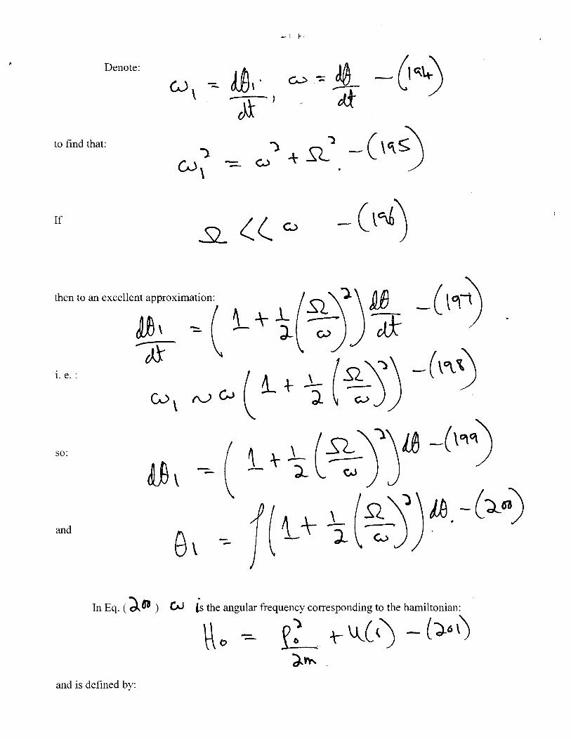
Denote:

to find that:

If

In Eq. ( ~ c11 ) C.V • ls the ang 1 ~ u ar lrequency c \ \ orresponding t h t\ - ") o t e hamiltonian:

0 - ~ t-\l._l() - (~6\)

and is defined by: d."'

In Eq. ( ~0 }):

therefore:

~ ----"'). Q

and

e\

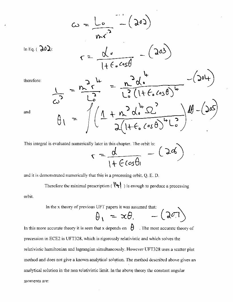
This integral is evaluated numerically later in this chapter. The orbit is:

rJ - -=------:----\ t EcosB,

and it is demonstrated numerically that this is a precessing orbit, Q. E. D.

Therefore the minimal prescription ( \'t\ ) is enough to produce il precessing

orbit.

In the x ilieory of previous 9~ pa:s i~ae ~sumed ili: ( J_ 0 .1)

In this more accurate theory it is seen that X depends on e . The most accurate theory of

precession in ECE2 is UFT328, which is rigorously relativistic and which solves the

relativistic hamiltonian and lagrangian simultaneously. However UFT328 uses a scatter plot

method and does not give a known analytical soh~tion. The method described above gives an

analytical solution in the non relativistic limit. In the above theory the constant angular

momenta are:

- (:lo~

the half right latitudes are: J.

_! -=- L ..., , \}._ - ") fr\ (s-

f\-

and the eccentricities are:

and

--

In general:

and this integral can be valuated analytically as shown later in this chapter. If it is assumed

that:

then:

)C.

and the orbit can be put into the form of an orbit of x theory { 1 - 12}:

\ -=- J, . _( ").ll.t-)

\t f (dJ (?c6) The orbit ( ~Ob ) is graphed later in this chapter and is shown to precess, Q. E.

D. It is generated by the orbital Lorentz force equation:

f -=- ~r·-=- -~m& i., +_~.Jy_d -Y't>i. ~_g_ -(:l~J - <~ ~t

in which the canonical momentum is:

"'-~ -- !_ -\- Vh. ;(_') _- (Hr) In the absence of a gravitomagnetic vector potential v Eq. (} \ t ) reduces to the Leibnitz

force equation: •, l "')) rt\ (; R

in which:

1=- "" ' - 't - '('" ----=-C r 6 e ":-- - V'c-.-. --('"

\ ~'~ J -•• ---

<k.'L -Jl

_()t<t) ( J_\ '\)

(.

Therefore the Leibnitz equation is:

-=- r( <) - ( ')_~~ and can be transfromed to the Binet equation:

The Leibnitz equation give the non precessing conic section:

( - ~

- r.-_/ f (<) - (:P~ c

To develop this equation consider the Lagran d . . ge envattve:

~'-! ?< ""- J'ix .-\- ~}.IV- -\- - .. - (_)~ '\ J1 d\: 6t )X :J

then to first order: ~')(_- ~ ~ -t-l~. ~ \~ -(:l)$\ ~ell- at -) -:;

where ~ -:.- ~ ~ -\-L ~ ~ ~ ~ - ( :1")() -- ~r\: ~t -- ?Jt --·

It follows that:

and

and:

for a planar orbit. Therefore the orbital Lorentz fi . orce equatiOn becomes:

•

- -=- - ~m& ~("- (g_. ~- ~d {"')

-\fh\ - ---

in which the canonic:m~men~~: ~ ( '{_ >, ~~) -:_ ~ ( g~ + '{ ~)

- -C~) The lagrangian corresponding to this general equation is developed in Note 348(3).

The hamiltonian ( \~ ) and the orbit ( }o~ ) are based on the assumption of a

uniform gravitomagnetic field defined by:

--=-- ~ ')<.. )!__) _( ",)__\~)

- l- ..sl ~ -' - (__ ).bi'l - d.-- . /

and:

As in Note 34 7(2):

"). - ' SL """ ' . .sL. ~ ~ '-J"o - ~ - -

which can be written as:

\ ---\+.

Sl) /-(~·i)(~·£) -( ).~')

i ~)~("~-.~~~-\A(()- (u~ _ v C<) -C),

in which the conserved angular momentum is:

"). - (~:1\ L -=--- \'),. < a . LJ

The other Euler Lagr1iuation i~ ~-) t _ ( ")_ ~) ~ Kd<

which gives the force equation: ( ~ - ~ ( r)- _Q ")) \ - {~ f(~c:.-~~-~~ ~

in which: { YhJ- c ").4$" "'\ 1r -=- -~MJs f ~ -~____, - '_} lA ) -":) '

' (

This is the Lorentz force equation of the precessing orbit ( l.d.o ), and as in Note 348(5)

can be transformed to the precessional Binet equation: