Γ-type estimates for the one-dimensional Allen-Cahn’s action

Giovanni Bellettini∗ Al-hassem Nayam† Matteo Novaga‡

Abstract

In this paper we prove an asymptotic estimate, up to the second order included, onthe behaviour of the one-dimensional Allen-Cahn’s action functionals, around a periodicfunction with bounded variation and taking values in {±1}. The leading term of thisestimate justifies and confirms, from a variational point of view, the results of Fusco-Hale[11] and Carr-Pego [8] on the exponentially slow motion of metastable patterns coexistingat the transition temperature.

1 Introduction

In this paper we are interested in the asymptotic behaviour as ε→ 0+ of the one-dimensionalAllen-Cahn’s action functionals

Fε(u) :=∫

T

(ε

2(u′)2 +

W (u)ε

)dx,

where T is the one-dimensional unit torus, W is a smooth double well potential with zeroesat ±1, and u : T → R. These functionals arise in several models of phase transitions inmaterials science, see for instance [4, 12, 13, 11, 8] and references therein. In particular, twophases u = ±1, coexisting at the transition temperature, exhibit metastable patterns whichslowly evolve according to the L2-gradient flow of Fε,

ut = ε2uxx −W ′(u), (1.1)

where a time rescaling has been performed. Equation (1.1) is perhaps the simplest partialdifferential equation modelling nonlinear relaxation to equilibrium in the presence of com-peting stable states. In [11, 8] the authors showed that, as ε → 0+, a solution u of (1.1) islocally equal to ±1 and the transition points evolve, exponentially slowly, in accordance to aspecific system of ODEs (see [11, Eq. (3.11)] and [8, Eq. (1.2)]). The exponential speed isdictated by the qualitative properties of W , in particular by its nondegeneracy at ±1.In this paper we aim to provide a variational couterpart of the dynamical results of [11, 8],recovering an analogous ODEs system obtained as a by-product of the behaviour, at the∗Dipartimento di Matematica, Universita di Roma Tor Vergata, via della Ricerca Scientifica 1, 00133 Roma,

Italy. E-mail: belletti@mat.uniroma2.it†The Abdus Salam International Center of Theoretical Physics-ICTP, Mathematics Section, Strada

Costiera 11, 34100, Trieste, Italy. E-mail: anayam@ictp.it‡Dipartimento di Matematica, Universita di Pisa, largo Pontecorvo 5, 56127 Pisa, Italy E-mail: no-

vaga@dm.unipi.it

1

leading order, of the action functionals Fε for ε << 1, around piecewise constant functionsu with values in {±1}, which correspond to the metastable patterns in the two-phase modeldescribed above. It is well-known [10, 14] that the sequence (Fε) is equicoercive in L1(T) andΓ-L1(T)-converges, as ε→ 0+, to the functional F0 : L1(T)→ [0,+∞] defined as

F0(u) :={N(u)σ if u ∈ BV (T; {±1}),+∞ otherwise,

(1.2)

where N(u) is the number of jump points of u, and where

σ := inf{∫

R

(12

(v′)2 +W (v))dy : v ∈ H1

loc(R), v(0) = 0, limy→±∞

v(y) = ±1}

(1.3)

is sometimes called surface tension.The main results of this paper are the following asymptotic estimates. Firstly (Theorem 6.1)we prove that

Fε(vε) ≥N(v)σ − α+κ2+

N(v)∑k=1

e−α+dεkε − α−κ2

−

N(v)∑k=1

e−α−dεkε

+ o

N(v)∑k=1

e−α+dεkε

+ o

N(v)∑k=1

e−α−dεkε

(1.4)

as ε → 0+, where (vε) is any sequence converging to v ∈ BV (T; {±1}) in L1(T), α±, κ±are constants1 depending on W , in particular α± :=

√W ′′(±1), and dεk is the distance

between the k-th and the (k + 1)-th transition of vε (see (5.9) and (6.2)). Notice that theterms appearing on the right-hand side of (1.4) scale differently in ε, as soon as the limitsdk(v) := limε d

εk are different for different k’s, and in particular we cannot substitute the

approximate distance dεk with the distance dk(v) = xk+1(v)− xk(v) between the consecutivek-th and (k + 1)-th jump point of the limit function v. Estimate (1.4) is sharp, in the sensethat for any v ∈ BV (T; {±1}) there exists a sequence (vε) such that the equality holds in(1.4) (Theorem 6.5).Secondly (Theorem 8.1) we show that if W is a parabola near ±1 then we can improve (1.4),obtaining the (sharp) estimate

Fε(vε) ≥N(v)σ − α+κ2+

N(v)∑k=1

e−α+dεkε − α−κ2

−

N(v)∑k=1

e−α−dεkε

+ o

N(v)∑k=1

e−3α+

2

dεkε

+ o

N(v)∑k=1

e−3α−

2

dεkε

.

(1.5)

Observe that (1.5) provides a sort of second order asymptotic expansion (with vanishingsecond order term) of Fε around functions v ∈ BV (T; {±1}), which is reminiscent of a Γ-expansion of Fε in the sense of [1, 2, 5, 6]. However, our results cannot be straightforwardly

1κ± are defined in (3.7), (3.8).

2

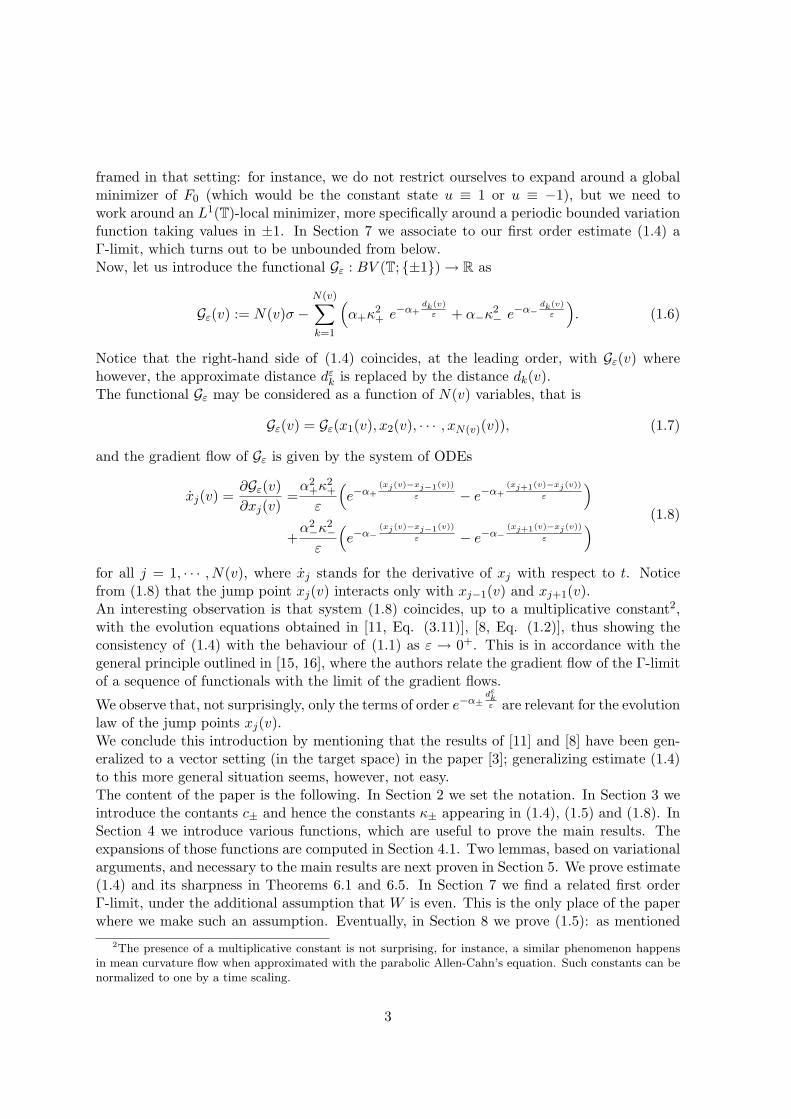
framed in that setting: for instance, we do not restrict ourselves to expand around a globalminimizer of F0 (which would be the constant state u ≡ 1 or u ≡ −1), but we need towork around an L1(T)-local minimizer, more specifically around a periodic bounded variationfunction taking values in ±1. In Section 7 we associate to our first order estimate (1.4) aΓ-limit, which turns out to be unbounded from below.Now, let us introduce the functional Gε : BV (T; {±1})→ R as

Gε(v) := N(v)σ −N(v)∑k=1

(α+κ

2+ e−α+

dk(v)

ε + α−κ2− e−α−

dk(v)

ε

). (1.6)

Notice that the right-hand side of (1.4) coincides, at the leading order, with Gε(v) wherehowever, the approximate distance dεk is replaced by the distance dk(v).The functional Gε may be considered as a function of N(v) variables, that is

Gε(v) = Gε(x1(v), x2(v), · · · , xN(v)(v)), (1.7)

and the gradient flow of Gε is given by the system of ODEs

xj(v) =∂Gε(v)∂xj(v)

=α2

+κ2+

ε

(e−α+

(xj(v)−xj−1(v))

ε − e−α+(xj+1(v)−xj(v))

ε

)+α2−κ

2−

ε

(e−α−

(xj(v)−xj−1(v))

ε − e−α−(xj+1(v)−xj(v))

ε

) (1.8)

for all j = 1, · · · , N(v), where xj stands for the derivative of xj with respect to t. Noticefrom (1.8) that the jump point xj(v) interacts only with xj−1(v) and xj+1(v).An interesting observation is that system (1.8) coincides, up to a multiplicative constant2,with the evolution equations obtained in [11, Eq. (3.11)], [8, Eq. (1.2)], thus showing theconsistency of (1.4) with the behaviour of (1.1) as ε → 0+. This is in accordance with thegeneral principle outlined in [15, 16], where the authors relate the gradient flow of the Γ-limitof a sequence of functionals with the limit of the gradient flows.

We observe that, not surprisingly, only the terms of order e−α±dεkε are relevant for the evolution

law of the jump points xj(v).We conclude this introduction by mentioning that the results of [11] and [8] have been gen-eralized to a vector setting (in the target space) in the paper [3]; generalizing estimate (1.4)to this more general situation seems, however, not easy.The content of the paper is the following. In Section 2 we set the notation. In Section 3 weintroduce the contants c± and hence the constants κ± appearing in (1.4), (1.5) and (1.8). InSection 4 we introduce various functions, which are useful to prove the main results. Theexpansions of those functions are computed in Section 4.1. Two lemmas, based on variationalarguments, and necessary to the main results are next proven in Section 5. We prove estimate(1.4) and its sharpness in Theorems 6.1 and 6.5. In Section 7 we find a related first orderΓ-limit, under the additional assumption that W is even. This is the only place of the paperwhere we make such an assumption. Eventually, in Section 8 we prove (1.5): as mentioned

2The presence of a multiplicative constant is not surprising, for instance, a similar phenomenon happensin mean curvature flow when approximated with the parabolic Allen-Cahn’s equation. Such constants can benormalized to one by a time scaling.

3

above, we are able to show this estimate supposing that W is a parabola near its minimumpoint, and this makes easy to treat the various singular integrals involved (in particular, thederivative of the function D+, defined in (4.5), evaluated at the point s = 1.

2 Notation

The assumptions on the double well potential W are the following:

(W1) W : R→ [0,+∞) and W ∈ C∞(R);

(W2) W−1(0) = {±1};

(W3) W ′′(±1) > 0. We set

α+ :=√W ′′(1), α− :=

√W ′′(−1). (2.1)

Notice that we do not suppose that W is even. We define

β± := W ′′′(±1).

A Taylor expansion around s = 1 gives

2W (s) = α2+(1− s)2

[1 +

β+

3α2+

(s− 1)]

+ o((1− s)3

)as s→ 1−, (2.2)

and similarly in a right neighborhood of −1 with α− replacing α+ and β− replacing β+.From (2.2) it follows 1√

2W (s))= 1

α+(1−s)

(1 + β+

6α2+

(1− s) + o(1− s))

as s→ 1−, so that

1√2W (s))

− 1α+(1− s)

=β+

6α3+

+ ρ(s), (2.3)

where the reminder

ρ : [0, 1]→ R is continuous, lims→1−

ρ(s) = 0.

We defineφ(η) :=

∫ η

−1

√2W (s) ds, η ∈ [−1, 1], (2.4)

It is known that σ in (1.3) satisfies

σ = φ(1) = σ− + σ+,

where we have set

σ− :=∫ 0

−1

√2W (s) ds, σ+ :=

∫ 1

0

√2W (s) ds.

Remark 2.1. Our assumptions on W ensure that for η ∈ (0, 1) (resp. η ∈ (−1, 0)) sufficientlyclose to 1 (resp. to −1) we have

W (η) < W (s), s ∈ (0, η) (resp. s ∈ (η, 0)),

and W ′(η) < 0 (resp. W ′(η) > 0).

4

2.1 Periodic BV functions

Let T be the one-dimensional unit torus. We denote by BV (T; {±1}) the space of functionsof bounded variation in T taking values ±1. For a function u ∈ BV (T; {±1}) with nonemptyjump set S(u) ⊂ T, we write S(u) = {x1(u), · · · , xN(u)(u)}, where N(u) ∈ (0,+∞) is thenumber of the jump points of u, and

x1(u) < x2(u) < · · · < xN(u)(u) < xN(u)+1(u) := x1(u). (2.5)

We let N+(u) be the number of increasing jumps from −1 to 1 (resp. N−(u) be the numberof decreasing jumps from 1 to −1). Due to the periodicity of functions in BV (T; {±1}), N(u)is even (or zero) and N+(u) = N−(u). If S(u) = ∅ we set N(u) = N+(u) = N−(u) = 0.

Definition 2.2. Let u ∈ BV (T; {±1}) be nonconstant. We define{dk(u) := xk+1(u)− xk(u), k = 1, · · · , N(u)− 1,dN(u) := 1− (xN(u) − x1(u)) = d0(u),

(2.6)

andI+(u) :=

{k ∈ {1, · · · , N(u)} : u jumps from − 1 to 1 at xk(u)

},

I−(u) :={1, · · · , N(u)} \ I+(u).

2.2 The functionals Fε and the minimizer γ

For any ε ∈ (0, 1) let Fε : L1(T)→ [0,+∞] be defined by

Fε(u) :=

∫

T

(ε

2(u′)2 +

W (u)ε

)dx if u ∈ H1(T) and W (u) ∈ L1(T),

+∞ otherwise.(2.7)

When I is a measurable subset of T, we denote by Fε(·, I) the localization of Fε(·) on I(obtained by replacing T with I in (2.7)) and we set Fε(·,T) = Fε(·).If J ⊂ R is a bounded interval and v ∈ H1(J), we set

F(v, J) :=∫J

(12

(v′)2 +W (v))dy, (2.8)

and for v ∈ H1loc(R), we let F(v) :=

∫R(

12(v′)2 +W (v)

)dy.

It is well-known that the infimum in (1.3) is a minimum and is attained by the functionγ ∈ C∞(R) solving {

γ′ =√

2W (γ) in R,γ(0) = 0.

(2.9)

5

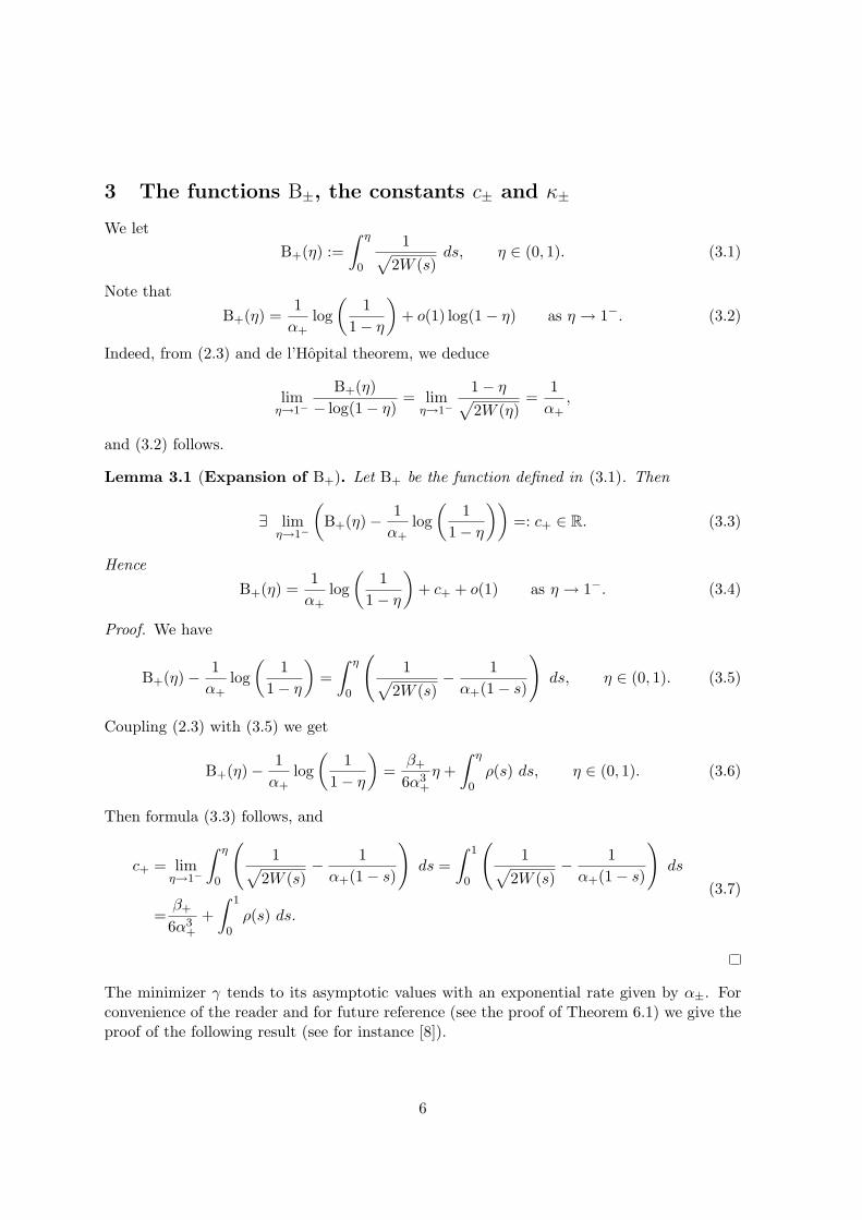
3 The functions B±, the constants c± and κ±

We letB+(η) :=

∫ η

0

1√2W (s)

ds, η ∈ (0, 1). (3.1)

Note that

B+(η) =1α+

log(

11− η

)+ o(1) log(1− η) as η → 1−. (3.2)

Indeed, from (2.3) and de l’Hopital theorem, we deduce

limη→1−

B+(η)− log(1− η)

= limη→1−

1− η√2W (η)

=1α+

,

and (3.2) follows.

Lemma 3.1 (Expansion of B+). Let B+ be the function defined in (3.1). Then

∃ limη→1−

(B+(η)− 1

α+log(

11− η

))=: c+ ∈ R. (3.3)

Hence

B+(η) =1α+

log(

11− η

)+ c+ + o(1) as η → 1−. (3.4)

Proof. We have

B+(η)− 1α+

log(

11− η

)=∫ η

0

(1√

2W (s)− 1α+(1− s)

)ds, η ∈ (0, 1). (3.5)

Coupling (2.3) with (3.5) we get

B+(η)− 1α+

log(

11− η

)=

β+

6α3+

η +∫ η

0ρ(s) ds, η ∈ (0, 1). (3.6)

Then formula (3.3) follows, and

c+ = limη→1−

∫ η

0

(1√

2W (s)− 1α+(1− s)

)ds =

∫ 1

0

(1√

2W (s)− 1α+(1− s)

)ds

=β+

6α3+

+∫ 1

0ρ(s) ds.

(3.7)

The minimizer γ tends to its asymptotic values with an exponential rate given by α±. Forconvenience of the reader and for future reference (see the proof of Theorem 6.1) we give theproof of the following result (see for instance [8]).

6

Corollary 3.2 (Asymptotic behaviour of γ). There exist the limits

limy→+∞

1− γ(y)e−α+y

=: κ+ ∈ (0,+∞), limy→−∞

1 + γ(y)eα−y

=: κ− ∈ (0,+∞). (3.8)

Proof. We consider the case y > 0, the case y < 0 being similar. From (2.9) it follows∫ y

0

γ′√2W (γ)

dz = B+(γ(y)) = y, y > 0. (3.9)

Therefore, using (3.4) we find y = − 1α+

log(1 − γ(y)) + c+ + o(1) as y → +∞. This impliesthe assertion in (3.8) with

κ+ = eα+c+ . (3.10)

We set B−(η) :=∫ 0η

1√2W (s)

ds for η ∈ (−1, 0), and

c− := limη→1−

∫ η

0

(1√

2W (−s)− 1α−(1 + s)

)ds, κ− := eα−c− .

4 The functions Q±, A±, D±, L±From Remark 2.1 we have that the function

Q+(η) :=∫ η

0

1√2W (s)− 2W (η)

ds, η ∈ (0, 1) close enough to 1 (4.1)

is well defined (one checks that 1√2W (·)−2W (η)

∈ L1(0, η)).

We letA+(η) :=

1α+

∫ η

0

1√(1− s)2 − (1− η)2

ds, η ∈ (0, 1). (4.2)

Setting 1 − η = ξ, changing variable with 1 − s = t and then t/ξ = x we get A+(η) =1α+

∫ 11−η

11√x2−1

dx. With a direct integration we have

A+(η) =1α+

log

(1− η

1−√

1− (1− η)2

), η ∈ (0, 1). (4.3)

Hence3

A+(η) =1α+

log(

21− η

)+ o(1) as η → 1−. (4.4)

For η ∈ (0, 1) sufficiently close to 1, we also consider the difference

D+(η) := Q+(η)−A+(η). (4.5)3Notice that if we put η = 1 inside the integrand of (4.2) we get 1

α+

R η0

11−s ds, which is not equal to the

leading term on the right hand side of (4.4).

7

Finally

L+(η) :=∫ η

0

√2W (s)− 2W (η) ds, η ∈ (0, 1] close enough to 1, (4.6)

Notice thatlimη→1−

L+(η) = L+(1) = σ+,

andL′+(η) = −W ′(η)Q+(η), η ∈ (0, 1) close enough to 1. (4.7)

We set Q−(η) :=∫ 0η

1√2W (s)−2W (η)

ds, L−(η) :=∫ 0η

√2W (s)− 2W (η) ds, and D−(η) :=

Q−(η)−A−(η) for η ∈ (−1, 0) sufficiently close to−1, whereA−(η) := 1α−

∫ 0η

1√(1−s)2−(1−η)2

ds

for η ∈ (−1, 0).

4.1 Expansions of D+, Q+ and L+

We shall need the following result.

Lemma 4.1 (Expansion of D+). Let c+ be as in (3.3). Then

limη→1−

D+(η) = c+ = D+(1). (4.8)

Proof. Recalling (2.2), write

f(x) := 2W (x)− α2+(1− x)2 − β+

3(x− 1)3, x ∈ R.

For s < η < 1 we write f(s)− f(η) = f ′(ξ)(s− η) for a suitable ξ ∈ (s, η): for s sufficientlyclose to 1 we deduce

2W (s)− 2W (η)

=α2+

((1− s)2 − (1− η)2

)+β+

3

((s− 1)3 − (η − 1)3

)+(2W ′(ξ) + 2α2

+(1− ξ)− β+(1− ξ)2)(s− η)

=α2+

((1− s)2 − (1− η)2

)(1 +

β+

3α2+

ψ(s, η) +R(s, η)),

(4.9)

whereψ(s, η) =

(s− 1)3 − (η − 1)3

(1− s)2 − (1− η)2= −(1− s)2 + (1− s)(1− η) + (1− η)2

(1− s) + (1− η),

R(s, η) =

(2W ′(ξ) + 2α2

+(1− ξ)− β+(1− ξ)2)

α2+ (s+ η − 2)

.

(4.10)

Since 1− η ≤ 1− s we haveψ(s, η) ≤ 3(1− s). (4.11)

8

Taylor expanding W ′ around s = 1, we have

2W ′(ξ) + 2α2+(1− ξ)− β+(1− ξ)2 =

W′′′′

(ζ)6

,

for a suitable ζ ∈ (ξ, 1). Hence

R(s, η) =O((1− ξ)3

)2− (s+ η)

= O((1− s)2

).

It then certainly follows from (4.9)

1√2W (s)− 2W (η)

=1 +O(1− s)

α+

√(1− s)2 − (1− η)2

.

Therefore, for s < η and as (s, η)→ (1−, 1−),

1√2W (s)− 2W (η)

− 1α+

√(1− s)2 − (1− η)2

=O(1− s)√

(1− s)2 − (1− η)2. (4.12)

For η ∈ (0, 1) sufficiently close to 1 we have

D+(η) =∫ η

0

(1√

2W (s)− 2W (η)− 1α+

√(1− s)2 − (1− η)2

)ds

= η

∫ 1

0

(1√

2W (sη)− 2W (η)− 1α+

√(1− sη)2 − (1− η)2

)ds.

(4.13)

From (4.12) applied with sη in place of s it follows∣∣∣∣∣ 1√2W (sη)− 2W (η)

− 1α+

√(1− sη)2 − (1− η)2

∣∣∣∣∣ ≤ C(1− sη)√(1− sη)2 − (1− η)2

=C√

1−(

1−η1−sη

)2,

for a suitable absolute positive constant C. Since the function η ∈ (0, 1) → 1r1−“

1−η1−sη

”2

is decreasing, the integrands on the right member of (4.13) are equiintegrable. Thus, byLebesgue’s dominated convergence theorem, we can pass to the limit in (4.13) as η → 1− andobtain

limη→1−

D+(t) =∫ 1

0

(1√

2W (s)− 1α+

√(1− s)2

)ds = c+. (4.14)

Lemma 4.2 (Expansion of Q+ at first order). Let Q+ be the function defined in (4.1).Then

Q+(η) =1α+

log(

11− η

)+

log 2α+

+ c+ + o(1) as η → 1−. (4.15)

9

Proof. Using (4.4) and (4.5) we have

Q+(η) =1α+

log(

21− η

)+D+(1) + o(1) as η → 1−, (4.16)

and the assertion follows from (4.8).

Lemma 4.3 (Expansion of L+ at first order). Let L+ be the function defined in (4.6).Then

L+(η) =σ+ −α+

2(1− η)2 log

(1

1− η

)− α+

2

(log(2κ+) +

12

)(1− η)2 + o

((1− η)2

)as η → 1−.

(4.17)

Proof. Using de l’Hopital theorem, (4.7), (2.2) and (4.15), we compute

limη→1−

L+(η)− σ+ + α+

2 (1− η)2 log(

11−η

)(1− η)2

=12

limη→1−

W ′(η)Q+(η) + α+(1− η) log(

11−η

)− α+

2 (1− η)

1− η

=12

limη→1−

−α2+(1− η)

[1α+

log(

11−η

)+ log 2

α++ c+

]+ α+(1− η) log

(1

1−η

)− α+

2 (1− η)

1− η

=− α+

2

[log 2 + α+c+ +

12

].

Then formula (4.17) follows, recalling also (3.10).

We shall use expansions (4.15) and (4.17) in formulas (6.13) and (6.16) below.

5 Two useful lemmas

In this section we prove two useful lemma, which are preliminary for the results of Section 6.

10

Lemma 5.1 (The functions zε). Let v ∈ BV (T; {±1}) be a function with N(v) > 0. Forany k = 1, · · · , N(v) with k even, suppose that v = −1 in (xk−1(v), xk(v)) and v = 1 in(xk(v), xk+1(v)). For any k = 1, · · · , N(v), let (xεk) ⊂ T be a sequence of points convergingto xk(v) as ε→ 0+, where we set kεN(v)+1 := xε1. Let

s0 ∈ (−1, 0), (5.1)

and define

Aεk(s0) :={z ∈ H1(xεk, x

εk+1) : z(xεk) = 0, z(xεk+1) = 0, (−1)kz(x) ≥ s0 for any x ∈ (xεk, x

εk+1)

}.

Then there exists a function zε ∈ H1(T; (−1, 1)) with the following properties:

(i) for any k = 1, · · · , N(v)

F(zε, (xεk, x

εk+1)

)= min

z∈Aεk(s0)Fε(z, (xεk, x

εk+1)

); (5.2)

(ii) there is a positive constant C depending only on W and v such that

supε∈(0,1)

Fε(zε) ≤ C; (5.3)

(iii) for any k = 1, · · · , N(v) we have zε ∈ C1,1([xεk, xεk+1]);

(iv) for any k = 1, · · · , N(v) we have that, for ε ∈ (0, 1) sufficiently small, zε ∈ C∞(xεk, xεk+1)

is a classical solution to−εz′′ε + ε−1W ′(zε) = 0 in (xεk, x

εk+1),

zε(xεk) = zε(xεk+1) = 0,zε > 0 in (xεk, x

εk+1) if k is even,

zε < 0 in (xεk, xεk+1) if k is odd.

(5.4)

Morover, zεk is even with respect to the mid point of (xεk, xεk+1);

(v) for any k = 1, · · · , N(v)limε→0+

maxx∈[xεk,x

εk+1]|zε(x)| = 1. (5.5)

Proof. Given k = 1, · · · , N(v), the minimum problem on the right hand side of (5.2) has asolution zεk by direct methods. Hence4, setting

zε := zεk on [xεk, xεk+1], k = 1, · · · , N(v),

we have that zε satisfies (i); note that, by truncating with the constants −1 and 1, we cansuppose that zε(x) ∈ [−1, 1] for any x ∈ T.

4If a < b < c < d, u ∈ H1(a, c), v ∈ H1(c, d), and u(c) = v(c), then the function w defined in (a, d) asw := u in (a, b) and w := v in (c, d) belongs to H1(a, d).

11

Assertion (ii) follows by comparing Fε(zε) with the value of Fε, on each interval (xεk, xεk+1), of

a competitor which, for k even (resp. k odd) takes values in [0, 1] (resp. in [−1, 0]) and grows(resp. decreases) linearly from 0 to 1 (resp. from 0 to −1) in (xεk, x

εk + ε), it is 1 (resp. −1)

in (xεk + ε, xεk+1− ε), and then decreases (resp. grows) to 0 (resp. to −1) in (xεk+1− ε, xεk+1).Let us show (iii) and (iv). Without loss of generality, we fix k even. The minimality ofzε in (xεk, x

εk+1) entails −εz′′ε + ε−1W ′(zε) ≥ 0 in the distributional sense in (xεk, x

εk+1). It

follows that z′′ε ≤ ε−2 mins∈[−1,1]W′(s) in the distributional sense in (xεk, x

εk+1). Therefore

zε is semiconcave [7] in (xεk, xεk+1) and, even more, it is semiconcave in [xεk, x

εk+1]. As a

consequence, the inequality −εz′′ε + ε−1W ′(zε) ≥ 0 holds in [xεk, xεk+1] in the viscosity sense.

We also have that zε is classical solution to −εz′′ε + ε−1W ′(zε) = 0 in the set {zε > s0} ∩(xεk, x

εk+1) and, in particular, −εz′′ε + ε−1W ′(zε) ≤ 0 in the viscosity sense in {zε > s0} ∩

(xεk, xεk+1), so that

zε ∈ C1,1({zε > s0} ∩ (xεk, x

εk+1)

)∩ C∞

({zε > s0} ∩ (xεk, x

εk+1)

).

On {zε = s0} ∩ (xεk, xεk+1), the function zε has a minimum, and therefore −z′′ε ≤ 0 in the

viscosity sense. Coupled with the previous observation, we deduce

zε ∈ C1,1([xεk, xεk+1]).

The energy conservation implies that ε (z′ε)2

2 − ε−1W (zε) is constant in any interval containedin {zε > s0} ∩ (xεk, x

εk+1), therefore

ε(z′ε)

2

2− ε−1W (zε) is a constant e(zεk) in [xεk, x

εk+1]. (5.6)

In particularε−1W (zε) ≥ −e(zεk) in [xεk, x

εk+1]. (5.7)

We claim thatzε > s0 in [xεk, x

εk+1]. (5.8)

Suppose by contradiction that {zε = s0}∩(xεk, xεk+1) 6= ∅. From (5.6) it follows that −e(zεk) =

ε−1W (s0) because on the set {zε = s0} there holds z′ε = 0. We deduce from (5.7)

Fε(zε, (xεk, xεk+1)) ≥ ε−1W (s0)(xεk+1 − xεk) > C,

for ε ∈ (0, 1) sufficiently small depending only on v and s0, in contradiction with (5.3). Weconclude that {zε = s0} ∩ (xεk, x

εk+1) = ∅, and this proves our claim (5.8). Notice that the

same argument shows that zε cannot have critical points in {zε < 0} ∩ (xεk, xεk+1), hence in

particularzε > 0 in (xεk, x

εk+1).

The proof of the validity of the ordinary differential equation in (5.4) then follows, and henceby uniqueness zε(x) ∈ (−1, 1) for any x ∈ T.Let us show that zεk is even with respect to the mid point of (xεk, x

εk+1). Let x ∈ (xεk, x

εk+1) be

a point where zεk takes the maximum value in [xεk, xεk+1]. Observe that zεk(x) := zεk(2x − x)

solves the ordinary differential equation in (5.4), with zεk(x) = zεk(x) and zε′k (x) = zεk′(x) = 0.

Hence by uniqueness zεk = zεk. If by contradiction x is not the mid point of (xεk, xεk+1), we

have that zεk vanishes somewhere in (xεk, xεk+1), which is impossible, because zεk > 0 by (5.4).

Assertion (v) follows, because contradicting (5.5) would contradict estimate (5.3).

12

Note that assertions (ii)-(v) are valid independently of s0; we shall make use of s0 in thesecond case of the proof of the next lemma. We need the following preliminary observation.Let v ∈ BV (T; {±1}) and (vε) ⊂ H1(T) be a sequence converging to v in L1(T) as ε → 0+.The continuity of vε and the convergence of (vε) to v imply that, for any k = 1, · · · , N(v),there exists a sequence (xεk) ⊂ T of points converging to xk(v), such that

vε(xεk) = 0, (5.9)

where xεN(v)+1 := xε1.

Lemma 5.2 (Action comparison between vε and zε). Let v be as in Lemma 5.1. Let(vε) ⊂ H1(T) be a sequence converging to v in L1(T) as ε → 0+. For any k = 1, · · · , N(v),select a sequence (xεk) ⊂ T of points converging to xk(v) such that vε(xεk) = 0, where we haveset xεN(v)+1 := xε1. With s0 as in (5.1), let (zε) be the sequence of functions given by Lemma5.1. Then

Fε(vε, (xεk, xεk+1)) ≥ Fε(zε, (xεk, xεk+1)), k = 1, · · · , N(v) (5.10)

for ε ∈ (0, 1) small enough.

Proof. Without loss of generality, let us fix k even. We divide the proof into two cases.Case 1. vε ≥ s0 in (xεk, x

εk+1).

In this case we have that vε ∈ Aεk(s0), and (5.10) follows by the minimality of zε (see (5.2)).Case 2. Suppose that vε(x) < s0 for some x ∈ (xεk, x

εk+1).

We have

Fε(vε, (xεk, x

εk+1)

)≥∫

(xεk,xεk+1)

√2W (vε)|v′ε| dx =

∫(xεk,x

εk+1)|φ(vε)′| dx

≥ (φ(0)− φ(mεk)) + (φ(M ε

k)− φ(mεk)) + (φ(M ε

k)− φ(0))=2 (φ(M ε

k)− φ(mεk)) ,

where φ is defined in (2.4), and

M εk := max{vε(x) : x ∈ [xεk, x

εk+1]} > mε

k := min{vε(x) : x ∈ [xεk, xεk+1]}.

Since φ is strictly increasing and mεk < s0, we deduce

Fε(vε, (xεk, x

εk+1)

)≥ 2 (φ(M ε

k)− φ(s0)) ≥ 2 (φ(1)− φ(s0)) + o(1) (5.11)

as ε→ 0+, where in the last inequality we have used that limε→0+ ‖vε − 1‖L1(xεk,xεk+1) = 0.

For any k = 1, · · · , N(v)− 1 let now dεk := xεk+1 − xεk and dεN(v) := 1− (xεN(v) − xε1), so that

limε→0+ dεk = dk(v).Define

zεk(x) :=

γ(x−xεkε

)if x ∈ (xεk, x

εk + dεk

2 ),

γ(xεk+1−x

ε

)if x ∈ (xεk + dεk

2 , xεk+1),

13

where γ solves (2.9). We have zεk ∈ Aεk(s0) and, as ε→ 0+,

Fε(zεk, (x

εk, x

εk+1)

)= 2

(φ

(max

x∈[xεk,xεk+1]

zεk(x)

)− φ(0)

)= 2 (φ(1)− φ(0)) + o(1). (5.12)

In addition, by minimality,

Fε(zεk, (x

εk, x

εk+1)

)≥ Fε

(zε, (xεk, x

εk+1)

). (5.13)

Then (5.10) follows from (5.11), (5.12) and (5.13) provided ε > 0 is sufficiently small since,being φ strictly increasing and s0 ∈ (−1, 0),

Fε (vε, (xεk, xεk)) ≥2(φ(1)− φ(s0)) + o(1) > 2(φ(1)− φ(0))

=Fε(zεk, (xεk, x

εk+1)) + o(1) ≥ Fε(zεk, (xεk, xεk+1)) + o(1).

6 First order estimate for Fε

In this section we prove the first order expansion for Fε, in the sense specified by Theorems6.1 and Theorem 6.5.

Theorem 6.1 (First order estimate from below). Suppose that assumptions (W1) −(W3) hold. Let (vε) ⊂ H1(T) be a sequence converging in L1(T) to a non constant functionv ∈ BV (T; {±1}). Then, for any k = 1, · · · , N(v), there exists a sequence (dεk) satisfyinglimε→0+

dεk = dk(v) such that

Fε(vε) ≥N(v)σ − α+κ2+

N(v)∑k=1

e−α+dεkε − α−κ2

−

N(v)∑k=1

e−α−dεkε

+ o

N(v)∑k=1

e−α+dεkε

+ o

N(v)∑k=1

e−α−dεkε

as ε→ 0+.

(6.1)

Proof. Without loss of generality, we can assumeN(v) ≥ 2, and that v = −1 in (xk−1(v), xk(v))and v = 1 in (xk(v), xk+1(v)) for any k = 1, · · · , N(v), k even. For any k = 1, · · · , N(v) se-lect a sequence (xεk) of points of T satisfying limε→0+ xεk = xk(v) and equality (5.9), wherexεN(v)+1 := xε1.Now, let dεk be defined as{

dεk := xεk+1 − xεk, k = 1, · · · , N(v)− 1,dεN(v) := 1− (xεN(v) − x

ε1) =: dε0,

(6.2)

and set

Iεk(xεk) :=(xεk −

dεk−1

2, xεk +

dεk2

).

From inequality (5.10) of Lemma 5.2 it follows

14

Fε(vε) =N(v)∑k=1

Fε(vε, (xεk, x

εk+1)

)≥

N(v)∑k=1

Fε(zε, (xεk, x

εk+1)

)=Fε(zε) =

N(v)∑k=1

Fε (zε, Iεk(xεk)) ,

(6.3)

for ε ∈ (0, 1) small enough. With the change of variable x = εy + xεk we get

Fε (zε, Iεk(xεk)) =∫

1εIεk(0)

(ε2

2(z′ε(εy + xεk)

)2 +W (zε(εy + xεk)))dy, (6.4)

where1εIεk(0) =

(−dεk−1

2ε,dεk2ε

). (6.5)

Let wεk ∈ H1(

1εIεk(0)

)be the function defined as

wεk(y) := zε(εy + xεk), y ∈ 1εIεk(0), (6.6)

where we set wε0 := wεN(v). We deduce

Fε (zε, Iεk(xεk)) =∫

1εIεk(0)

(12

(wεk′(y))2 +W (wεk(y))

)dy = F

(wεk,

1εIεk(0)

), (6.7)

where F is defined in (2.8). Hence, from (6.3),

Fε(vε) ≥N(v)∑k=1

F(wεk,

1εIεk(0)

)=

∑k∈I+(v)

F(wεk,

1εIεk(0)

)+

∑k∈I−(v)

F(wεk,

1εIεk(0)

),

(6.8)

for ε ∈ (0, 1) small enough. Observe from (5.4) that wεk solves{−wεk ′′ +W ′(wεk) = 0 in

(−dεk−1

2ε ,dεk2ε

)\ {0},

wεk(0) = 0.(6.9)

Moreover, from (5.5) we get

limε→0+

∣∣∣∣wεk (−dεk−1

2ε

)∣∣∣∣ = limε→0+

∣∣∣∣wεk (dεk2ε

)∣∣∣∣ = 1. (6.10)

Define e(wεk−1) and e(wεk) as the (conserved) energy densities of wεk in(−dεk−1

2ε , 0)

and(

0, dεk

2ε

)respectively, namely

e(wεk−1) :=(wεk

′−(0))2

2−W (0) = −W

(wεk

(−dεk−1

2ε

))< 0,

e(wεk) :=(wεk

′+(0))2

2−W (0) = −W

(wεk

(dεk2ε

))< 0,

(6.11)

15

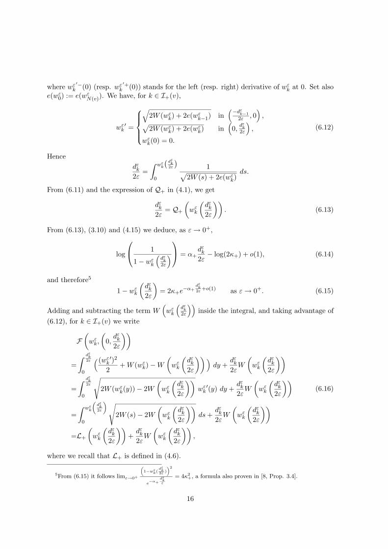
where wεk′−(0) (resp. wεk

′+(0)) stands for the left (resp. right) derivative of wεk at 0. Set alsoe(wε0) := e(wεN(v)). We have, for k ∈ I+(v),

wεk′ =

√

2W (wεk) + 2e(wεk−1) in(−dεk−1

2ε , 0),√

2W (wεk) + 2e(wεk) in(

0, dεk

2ε

),

wεk(0) = 0.

(6.12)

Hencedεk2ε

=∫ wεk

(dεk2ε

)0

1√2W (s) + 2e(wεk)

ds.

From (6.11) and the expression of Q+ in (4.1), we get

dεk2ε

= Q+

(wεk

(dεk2ε

)). (6.13)

From (6.13), (3.10) and (4.15) we deduce, as ε→ 0+,

log

1

1− wεk(dεk2ε

) = α+

dεk2ε− log(2κ+) + o(1), (6.14)

and therefore5

1− wεk(dεk2ε

)= 2κ+e

−α+dεk2ε

+o(1) as ε→ 0+. (6.15)

Adding and subtracting the term W(wεk

(dεk2ε

))inside the integral, and taking advantage of

(6.12), for k ∈ I+(v) we write

F(wεk,

(0,dεk2ε

))

=∫ dεk

2ε

0

((wεk′)2

2+W (wεk)−W

(wεk

(dεk2ε

)))dy +

dεk2εW

(wεk

(dεk2ε

))

=∫ dεk

2ε

0

√2W (wεk(y))− 2W

(wεk

(dεk2ε

))wεk′(y) dy +

dεk2εW

(wεk

(dεk2ε

))

=∫ wεk

„dεk2ε

«0

√2W (s)− 2W

(wεk

(dεk2ε

))ds+

dεk2εW

(wεk

(dεk2ε

))=L+

(wεk

(dεk2ε

))+dεk2εW

(wεk

(dεk2ε

)),

(6.16)

where we recall that L+ is defined in (4.6).

5From (6.15) it follows limε→0+

„1−wεk(

dεk2ε )

«2

e−α+

dεkε

= 4κ2+, a formula also proven in [8, Prop. 3.4].

16

Substituting (4.17) and (2.2) into (6.16) we deduce, using also (6.14) and (6.15),

F(wεk,

(0,dεk2ε

))

=σ+ −α+

2

(1− wεk

(dεk2ε

))2

log

1

1− wεk(dεk2ε

)

− α+

2

(log(2κ+) +

12

)(1− wεk

(dεk2ε

))2

+dεk2εα2

+

2

(1− wεk

(dεk2ε

))2

+ o

((1− wεk

(dεk2ε

))2)

=σ+ −α+

2

(log(2κ+) +

12− log(2κ+)

)(1− wεk

(dεk2ε

))2

+ o

((1− wεk

(dεk2ε

))2)

=σ+ − α+κ2+e−α+

dεkε + o

(e−α+

dεkε

)as ε→ 0+.With similar arguments one can prove that

F(wεk,

(−dεk−1

2ε, 0))

= σ− − α−κ2−e−α−

dεk−1ε + o

(e−α−

dεk−1ε

).

Hence, for k ∈ I+(v) we get

F(wεk,

1εIεk(0)

)= σ − α+κ

2+e−α+

dεkε − α−κ2

−e−α−

dεk−1ε + o

(e−α+

dεkε

)+ o

(e−α−

dεk−1ε

).

(6.17)Similarly, for k ∈ I−(v), we have

F(wεk,

1εIεk(0)

)= σ − α−κ2

−e−α−

dεkε − α+κ

2+e−α+

dεk−1ε + o

(e−α−

dεkε

)+ o

(e−α+

dεk−1ε

).

(6.18)From (6.8), (6.17) and (6.18) the assertion of the theorem follows.

Remark 6.2 (W even). When W is even, in order to prove Theorem 6.1 there is no needto introduce s0 as in (5.1), and there is no need to use Lemmas 5.1 and 5.2. Indeed, if W iseven, we can define zεk a a solution to (5.2) where s0 is replaced by 0, and we can directlyprove inequality (5.10), since

Fε(vε, (xεk, xεk+1)) = Fε(|vε|, (xεk, xεk+1)) ≥ Fε(zεk, (xεk, xεk+1)).

17

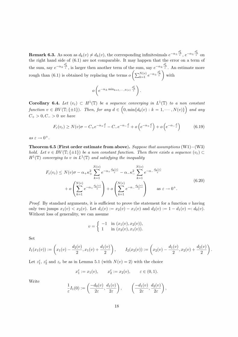
Remark 6.3. As soon as dk(v) 6= dh(v), the corresponding infinitesimals e−α±dεkε , e−α±

dεhε on

the right hand side of (6.1) are not comparable. It may happen that the error on a term of

the sum, say e−α±dεkε , is larger then another term of the sum, say e−α±

dεhε . An estimate more

rough than (6.1) is obtained by replacing the terms o(∑N(v)

k=1 e−α±dεkε

)with

o

(e−α±mink=1,··· ,N(v)

dεkε

).

Corollary 6.4. Let (vε) ⊂ H1(T) be a sequence converging in L1(T) to a non constantfunction v ∈ BV (T; {±1}). Then, for any d ∈

(0,min{dk(v) : k = 1, · · · , N(v)}

)and any

C+ > 0, C− > 0 we have

Fε(vε) ≥ N(v)σ − C+e−α+

dε − C−e−α−

dε + o

(e−α+

dε

)+ o

(e−α−

dε

)(6.19)

as ε→ 0+.

Theorem 6.5 (First order estimate from above). Suppose that assumptions (W1)−(W3)hold. Let v ∈ BV (T; {±1}) be a non constant function. Then there exists a sequence (vε) ⊂H1(T) converging to v in L1(T) and satisfying the inequality

Fε(vε) ≤ N(v)σ − α+κ2+

N(v)∑k=1

e−α+dk(v)

ε − α−κ2−

N(v)∑k=1

e−α−dk(v)

ε

+ o

N(v)∑k=1

e−α+dk(v)

ε

+ o

N(v)∑k=1

e−α−dk(v)

ε

as ε→ 0+.

(6.20)

Proof. By standard arguments, it is sufficient to prove the statement for a function v havingonly two jumps x1(v) < x2(v). Let d1(v) := x2(v) − x1(v) and d2(v) := 1 − d1(v) =: d0(v).Without loss of generality, we can assume

v ={−1 in (x1(v), x2(v)),1 in (x2(v), x1(v)).

Set

I1(x1(v)) :=(x1(v)− d2(v)

2, x1(v) +

d1(v)2

), I2(x2(v)) :=

(x2(v)− d1(v)

2, x2(v) +

d2(v)2

).

Let zε1, zε2 and zε be as in Lemma 5.1 (with N(v) = 2) with the choice

xε1 := x1(v), xε2 := x2(v), ε ∈ (0, 1).

Write1εI1(0) :=

(−d0(v)

2ε,d1(v)

2ε

),

(−d1(v)

2ε,d2(v)

2ε

),

18

and let wε1 ∈ H1(1εI1(0)) and wε2 = wε0 ∈ H1(1

εI2(0)) be defined as in (6.6). Then wε1 and wε2satisfy (6.11) and (6.12). We define

vε(x) :=

wε2

(x2(v)−x

ε

)if x ∈ I2(x2(v)),

wε1

(x−x1(v)

ε

)if x ∈ I1(x1(v)).

Then vε ∈ H1(T), (vε) converges to v in L1(T) as ε→ 0+, and

Fε(vε) = Fε(vε, I1(x1(v))) + Fε(vε, I2(x2(v))). (6.21)

With the change of variable y = x−x2(v)ε , we have Fε(vε, I2(x2(v))) = F

(wε2,

1εI2(0)

), and, as

in (6.16),

F(wε2,

(0,d2(v)

2ε

))=L+

(wε2

(d2(v)

2ε

))+d2(v)

2εW

(wε2

(d2(v)

2ε

)). (6.22)

Then the proof follows along the same lines as the proof of Theorem 6.1.

Remark 6.6. With slight modifications in the proof of Theorem 6.5, one can show that forany sequence (dεk) converging to dk(v), there exists a sequence (vε) ⊂ H1(T) converging to vin L1(T) and satisfying the equality in (6.1) with dεk = dk(v) for any k = 1, · · · , N(v).

Remark 6.7. From Theorems 6.1 and 6.5 it follows that, given γ > 0, for any v ∈BV (T; {±1}) with N(v) > 0 and for any sequence (vε) ∈ H1(T) such that vε → v in L1(T)as ε→ 0+, there holds

lim infε→0+

Fε(vε)−N(v)σεγ

≥ 0,

with the equality along a particular sequence. Hence the Γ-expansion of the functionals Fεin the sense of [5], whose zeroth-order is given by N(·)σ, contains no terms of order εγ forany γ > 0.

7 Γ-convergence

Throughout this short section, N ∈ N and m > 0 are fixed, and we assume for simplicitythat W is even. We set α := α− = α+ (see (2.1)) and κ := κ− = κ+ (see (3.10)). For anyε ∈ (0, 1] we define the functionals TN,mε : L1(T)→ (−∞,+∞] as

TN,mε (v) := eαmε

(Fε(v)−Nσ

).

Observe that TN,mε may take negative values.

19

Remark 7.1. Let (vε) ⊂ H1(T) be such that

supε∈(0,1]

TN,mε (vε) < +∞. (7.1)

Then supε∈(0,1]

Fε(vε) < +∞. Hence (vε) admits a (not relabeled) subsequence converging in

L1(T) to a function v ∈ BV (T; {±1}), and

N(v)σ ≤ Γ−L1(T) lim infε→0+

Fε(v) ≤ lim supε→0+

Fε(vε) ≤ Nσ,

where the last iequality follows from (7.1). Hence

N ≥ N(v).

Theorem 7.2 (First order Γ-limit). Suppose that assumptions (W1) − (W3) hold, andthat in addition W is even. Then the sequence (TN,mε ) Γ-L1(T)-converges, as ε→ 0+, to thefunctional TN,m : L1(T)→ [−∞,+∞] given by

TN,m(v) =

0 if v ∈ BV (T; {±1}), N = N(v) and m < m(v),−∞ if v ∈ BV (T; {±1}), N = N(v) and m ≥ m(v),+∞ if v ∈ BV (T; {±1}) and N < N(v),−∞ if v ∈ BV (T; {±1}) and N > N(v),+∞ if v ∈ L1(T) \BV (T; {±1}),

where, for any v ∈ BV (T; {±1}), we have set m(v) := min{dk(v) : k = 1, · · · , N(v)}.

Proof. Set T+ := Γ− L1(T) lim supε→0+

TN,mε and T− := Γ− L1(T) lim infε→0+

TN,mε . Let v ∈ L1(T),

and let (vε) ⊂ H1(T) be a sequence satisfying (7.1) and converging to v in L1(T). Thenv ∈ BV (T; {±1}) and N ≥ N(v), so that T−(v) = +∞ if

either v ∈ L1(T) \BV (T; {±1}) or v ∈ BV (T; {±1}) and N < N(v), (7.2)

and thereforeΓ− L1(T) lim

ε→0+TN,mε (v) = +∞ if v satisfies (7.2).

We can assume from now on that v ∈ BV (T; {±1}). The continuity of vε and the convergenceof (vε) to v imply that there exist an infinitesimal sequence (δε) ⊂ (0, 1) and, for any k =1, · · · , N(v), a sequence of points (xεk) ⊂ T, such that for any ε ∈ (0, 1),

|xk(v)− xεk| ≤ δε,

and (5.9) holds. From Theorem 6.1, (6.1), and dεk = xεk+1 − xεk ≥ xk+1(v) − xk(v) − 2δε ≥m(v)− 2δε, we have

Fε(vε) ≥ N(v)σ − 2ακ2#{k = 1, · · · , N(v) : dk(v) = m(v)

}e−α

m(v)−2δεε + o

(e−α

m(v)−2δεε

)

20

since the contribution due to the remaining jump points is of higher order. Moreover

TN,mε (vε) =eαmε

(Fε(vε)−Nσ

)≥eα

mε (N(v)−N)σ − 2ακ2#

{k = 1, · · · , N(v) : dk(v) = m(v)

}eα

m−m(v)+2δεε

+ o(eα

m−m(v)+2δεε

).

HenceN = N(v), m < m(v) ⇒ T−(v) ≥ 0. (7.3)

If now (vε) denotes the sequence constructed in Theorem 6.5, we have

TN,mε (vε) ≤ eαmε

(N(v)−N

)σ − 2ακ2

N(v)∑k=1

eαm−dk(v)

ε + o

N(v)∑k=1

eαm−dk(v)

ε

. (7.4)

Therefore, for a v satisfying (7.3), we have limε→0+ TN,mε (vε) = 0, hence T+(v) ≤ 0,which coupled with (7.3) gives

N < N(v), m < m(v) ⇒ Γ− L1(T) limε→0+

TN,mε (v) = 0.

If either N > N(v) or N = N(v) and m > m(v), from (7.4) it follows lim supε→0+ TN,mε (vε) =

−∞, so that T+(v) = −∞. Eventually, from the L1(T)-lower semicontinuity of T+, we deduce

N = N(v), m ≥ m(v) ⇒ T+(v) = −∞.

8 Second order estimate for Fε

This section is devoted to prove estimate (1.5). In what follows, beside the hypotheses on Wlisted at the beginning of Section 2, we shall suppose also that there exists δ ∈ (0, 1) so that

W (s) =α2−2

(1− s)2, s ∈ (−1− δ,−1 + δ),

W (s) =α2

+

2(1− s)2, s ∈ (1− δ, 1 + δ).

(8.1)

Notice that, in this case, we haveβ± = 0. (8.2)

21

Theorem 8.1 (Second order estimate from below). Suppose that assumptions (W1)−(W3) hold, and that in addition (8.1) holds. Let (vε), v, k and (dεk) be as in Theorem 6.1.Then

Fε(vε) ≥N(v)σ − α+κ2+

N(v)∑k=1

e−α+dεkε − α−κ2

−

N(v)∑k=1

e−α−dεkε

+ o

N(v)∑k=1

e−3α+

2

dεkε

+ o

N(v)∑k=1

e−3α−

2

dεkε

(8.3)

as ε→ 0+.

We start the proof of Theorem 8.1 with the following result.

Lemma 8.2 (Computation of D′+(1)). We have

D′+(1) := limη→1−

D′+(η) = 0. (8.4)

Proof. Using the additional assumption (8.1) on W , for η ∈ (1−δ, 1) we have for the functionD+ defined in (4.5),

D+(η) =∫ 1−δ

0

{1√

2W (s)− 2W (η)− 1α+

√(1− s)2 − (1− η)2

}ds,

and therefore D+ is of class C∞ in a left neighbourhood of η = 1. Differentiating under theintegral sign we get

D′+(η) =∫ 1−δ

0

{W ′(η)

(2W (s)− 2W (η))3/2+

1− ηα+((1− s)2 − (1− η)2)3/2

}ds,

and the assertion follows passing to the limit under the integral sign.

Corollary 8.3 (Second order expansion of Q+ and L+). We have

Q+(η) =1α+

log(

21− η

)+ c+ + o(1− η),

L+(η) =σ+ −α+

2(1− η)2 log

(1

1− η

)− α+

2

(log(2κ+) +

12

)(1− η)2 + o

((1− η)3

)as η → 1−.

(8.5)

as η → 1−.

Proof. The formula for Q+ follows from (4.16), (4.8) and Lemma 8.2. The formula for L+

follows by a direct computation as in the proof of Lemma 4.3, considering

limη→1−

L+(η)− σ+ + α+

2 (1− η)2 log(

11−η

)+ α+

2

(log(2κ+) + 1

2

)(1− η)2

(1− η)3,

applying de l’Hopital’s Theorem and using the expansion of Q+ in (8.5) instead of (4.15),and (8.2).

22

Following the notation of equations (6.15) and (6.14), we have the following expansions.

Lemma 8.4. Let k ∈ S+(v). Then

1− wε(dεk2ε

)= 2κ+e

−α+dεk2ε + o

(e−α+

dεkε

), (8.6)

and

log

1

1− wε(dεk2ε

) = α+

dεk2ε− log(2κ+) + o(1). (8.7)

Proof. We prove only the first expansion, the other being similar. From (3.10), (6.13) and(8.5) it follows

1− wε(dεk2ε

)= 2κ+e

−α+dεk2ε e

o

„1−wε

„dεk2ε

««. (8.8)

Hence, from (8.8) it follows

1− wε(dεk2ε

)= 2κ+e

−α+dεk2ε + o

(e−α+

dεkε

).

Now, let (vε), v, k and and dεk be as in Theorem 6.1. Following the notation and the proofof the same theorem (see in particular (6.16)), we have to expand the quantity

L+

(wεk

(dεk2ε

))+dεk2εW

(wεk

(dεk2ε

)). (8.9)

In view of the computations in the proof of Theorem 6.1, using (8.2) it is sufficient to isolate

the coefficients of the terms of order e−α+3dεk2ε in (8.9), and (8.3) follows, thus showing Theorem

8.1.We conclude the paper with following result, the proof of which follows along the same linesof Theorem 8.1, in a much simpler way.

Theorem 8.5 (Second order estimate from above). Suppose that assumptions (W1)−(W3) hold, and that in addition (8.1) holds. Let v and (vε) be as in Theorem 6.5. Then

Fε(vε) ≤N(v)σ − α+κ2+

N(v)∑k=1

e−α+dk(v)

ε − α−κ2−

N(v)∑k=1

e−α−dk(v)

ε

+ o

N(v)∑k=1

e−3α+

2

dk(v)

ε

+ o

N(v)∑k=1

e−3α−

2

dk(v)

ε

(8.10)

as ε→ 0+.

23

References

[1] G. Anzellotti, S. Baldo, Asymptotic development by Γ-convergence, Appl. Math. Opti-mization 27 (1993), 105-123.

[2] G. Anzellotti, S. Baldo, G. Orlandi, Γ-asymptotic development, the Cahn-Hilliard func-tional and curvatures, J. Math. Anal. Appl. 197 (1996), 908-924.

[3] F. Bethuel, G. Orlandi, D. Smets, Slow motion for gradient systems with equal depthmultiple-well potentials, J. Differ. Equations 250 (2011), 53–94.

[4] V. Bongiorno, L.E. Scriven, H.T. Davis, Molecular theory of fluid interfaces, J. ColloidInterface Sci. 57 (1976), 462-475.

[5] A. Braides, L. Truskinovsky, Asymptotic expansion by Γ-convergence, Cont. Mech.Therm. 20 (2008), 21-62.

[6] A. Braides, C.I. Zeppieri, Multiscale analysis of a prototypical model for the interactionbetween microstructure and surface energy, Interface Free Bound. 11 (2009), 61-118.

[7] P. Cannarsa and C. Sinestrari, Semiconcave Functions, Hamilton-Jacobi Equations, andOptimal Control, Progress in Nonlinear Differential Equations and Their Applications,58. Boston, Birkhauser, 2004.

[8] J. Carr, R.L. Pego, Metastable patterns in solutions of ut = ε2uxx − f(u), Comm. PureAppl. Math. 42 (1989), 523-576.

[9] G. Dal Maso, An introduction to Γ-convergence, Birkhauser, Boston (1993).

[10] E. De Giorgi, T. Franzoni, Su un tipo di convergenza variazionale, Atti Accad. Naz.Lincei Rend. Cl. Sci. Fis. Mat. Natur. 58 (1975), 842–850.

[11] G. Fusco, J.K. Hale, Slow motion manifolds, dormant instability, and singular perturba-tions, Dyn. Diff. Equation 1 (1989), 75-94.

[12] M.E. Gurtin, On the two-phase Stefan problem with interfacial energy and entropy, Arch.Ration. Mech. Anal. 96 (1986), 199–241.

[13] M.E. Gurtin, On phase transitions with bulk, interfacial, and boundary energy, Arch.Ration. Mech. Anal., 96 (1986), 243–264.

[14] L. Modica, S. Mortola, Un esempio di Γ−-convergenza, Boll. Un. Mat. Ital. 14B (1977),285-299.

[15] E. Sandier, S. Serfaty, Gamma-convergence of gradient flows with applications toGinzburg-Landau, Comm. Pure Appl. Math. 57 (2004), 1627–1672.

[16] S. Serfaty, Gamma-convergence of gradient flows on Hilbert and metric spaces and ap-plications, Disc. Cont. Dyn. Systems A 31 (2011), 1427–1451.

24