Введение в кластеризацию - sas...partitive clustering reference vectors...
TRANSCRIPT

Copyright © 2010, SAS Institute Inc. All rights reserved.
Введение в кластеризацию

2
Кластеризация
Кластеризация – процедура автоматического разбиения
некоторого множества объектов на группы (кластеры) на
основе степени их схожести
Кластеризация – обучение без учителя (целевая
переменная не требуется, нужны лишь характеристики
объектов)
Признаки «хорошего» кластера:
● близость объектов внутри кластера
● удаленность от остальных кластеров

3
Процедуры кластеризации в SAS/STAT
Variable SelectionVARCLUS
Plot DataPRINCOMP, MDS
PreprocessingACECLUS, STDIZE,
DISTANCE
Hierarchical ClusteringCLUSTER
Partitive Clustering
Parametric ClusteringFASTCLUS
Non-Parametric Clustering
MODECLUS
SAS/STAT содержит богатый набор процедур для подготовки
данных, широкий выбор алгоритмов кластеризации и
оценки результатов моделирования
НО... ЗАЧЕМ ВООБЩЕ НУЖНА КЛАСТЕРИЗАЦИЯ?

4
Example: Clustering for Customer Types
While you have thousands of customers, there are really
only a handful of major types into which most of your
customers can be grouped.
Bargain hunter
Man/woman on a mission
Impulse shopper
Weary parent
DINK (dual income, no kids)

5
Example: Clustering for Store Location
You want to open new grocery stores in the U.S.
based on demographics. Where should you locate
the following types of new stores?
low-end budget grocery stores
small boutique grocery stores
large full-service supermarkets

6
Профилирование кластеров
Профилирование – это попытка вывести «бытовой»
смысл группировки конкретных объектов в кластер
Цель – определить уникальные черты (или их
комбинации), характеризующие объекты в кластере

7
Виды кластеризации

8
Иерархическая кластеризация
Аггломеративная Дробящая

9
Partitive clustering
reference vectors (seeds)
X XX
X
Initial State
observations
Final State
XX X X
X
XX
X
PROBLEMS!
– make you guess the number of clusters present
– make assumptions about the shape of the clusters
– influenced by seed location, outliers, and order of reading
observations
– impossible to determine the optimal grouping, due to the
combinatorial explosion of potential solutions.

10
Partitive clustering: Heuristic Search
1. Generate an initial partitioning (based on the seeds)
of the observations into clusters.
2. Calculate the change in error produced by moving
each observation from its own cluster to each of the
other clusters.
3. Make the move that produces the greatest reduction.
4. Repeat steps 2 and 3 until no move reduces error.

11
Меры сходстваобъектов

12
Principles of a Good Similarity Metric
Properties of a good similarity metrics:
1. symmetry:
d(x,y) = d(y,x)
2. non-identical distinguishability:
d(x,y) 0 → x y
3. identical non-distinguishability:
d(x,y) = 0 → x = y
4. triangular inequality:
d(x,y) d(x,z) + d(y,z)
13
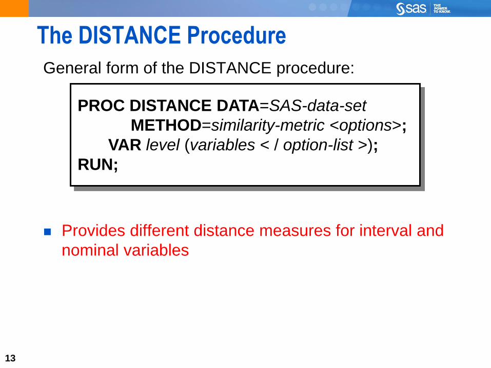
The DISTANCE Procedure
General form of the DISTANCE procedure:
Provides different distance measures for interval and
nominal variables
PROC DISTANCE DATA=SAS-data-set
METHOD=similarity-metric <options>;
VAR level (variables < / option-list >);
RUN;

14
Simple popular Distance Metrics (Interval Vars)
Euclidean distance
City Block Distance
Correlation
k
i
iiE wxD1
2wx
d
i
iiM wxD1
1

15
Distance between Clusters: density-based
During more complex clustering processes one must not
only calculate distances between objects, but also
calculate distances between sub-clusters
Density-based methods define similarity as the distance
between derived density “bubbles” (hyper-spheres).
similarity
Density estimate 1
(cluster 1)Density estimate 2
(cluster 2)

16
Оценка качествакластеризации

17
От кластеров к классам
Perfect
Типичные кластеры
Это – не
кластеризация
Идеальные кластеры
Если часть объектов выборки относится к разным классам, то это можно использовать для оценки качества кластеризации

18
От кластеров к вероятностям классов
The probability that a cluster represents a given class is
given by the cluster’s proportion of the row total.
Frequency Probability
19
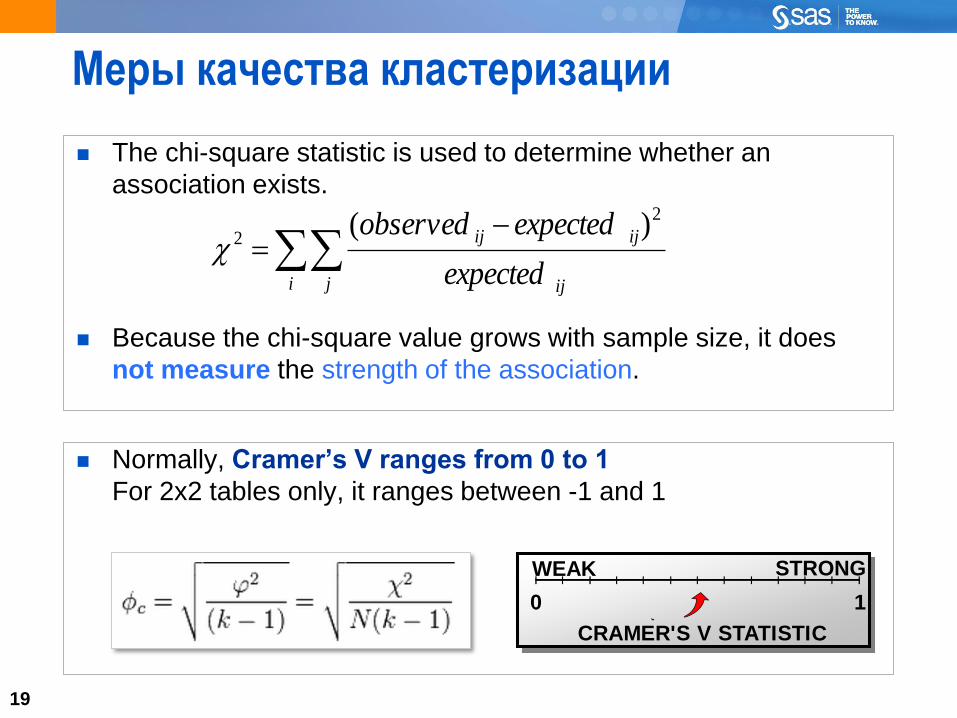
Меры качества кластеризации
The chi-square statistic is used to determine whether an
association exists.
Because the chi-square value grows with sample size, it does
not measure the strength of the association.
i j ij
ijij
expected
expectedobserved 2
2) (
Normally, Cramer’s V ranges from 0 to 1
For 2x2 tables only, it ranges between -1 and 1
WEAK STRONG
0 1
CRAMER'S V STATISTIC

20
Подготовка и разведочный анализ
данных

21
The Challenge of Opportunistic Data
Getting anything useful out of tons of data
22
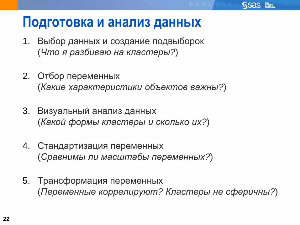
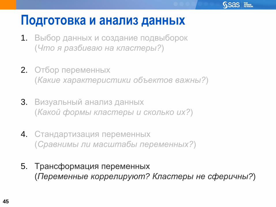
Подготовка и анализ данных1. Выбор данных и создание подвыборок
(Что я разбиваю на кластеры?)
2. Отбор переменных
(Какие характеристики объектов важны?)
3. Визуальный анализ данных
(Какой формы кластеры и сколько их?)
4. Стандартизация переменных
(Сравнимы ли масштабы переменных?)
5. Трансформация переменных
(Переменные коррелируют? Кластеры не сферичны?)
22

23
Data and Sample Selection
Not necessary to cluster a large population if you use
clustering techniques that lend themselves to scoring
(for example: Ward’s, k-means)
It is useful to take a random sample for clustering and
score the remainder of the larger population
23
CLUSTER
IT, BEBE!
THEN SCORE
THESE GUYS!

24
Подготовка и разведочный анализ
данных
Отбор переменных
25
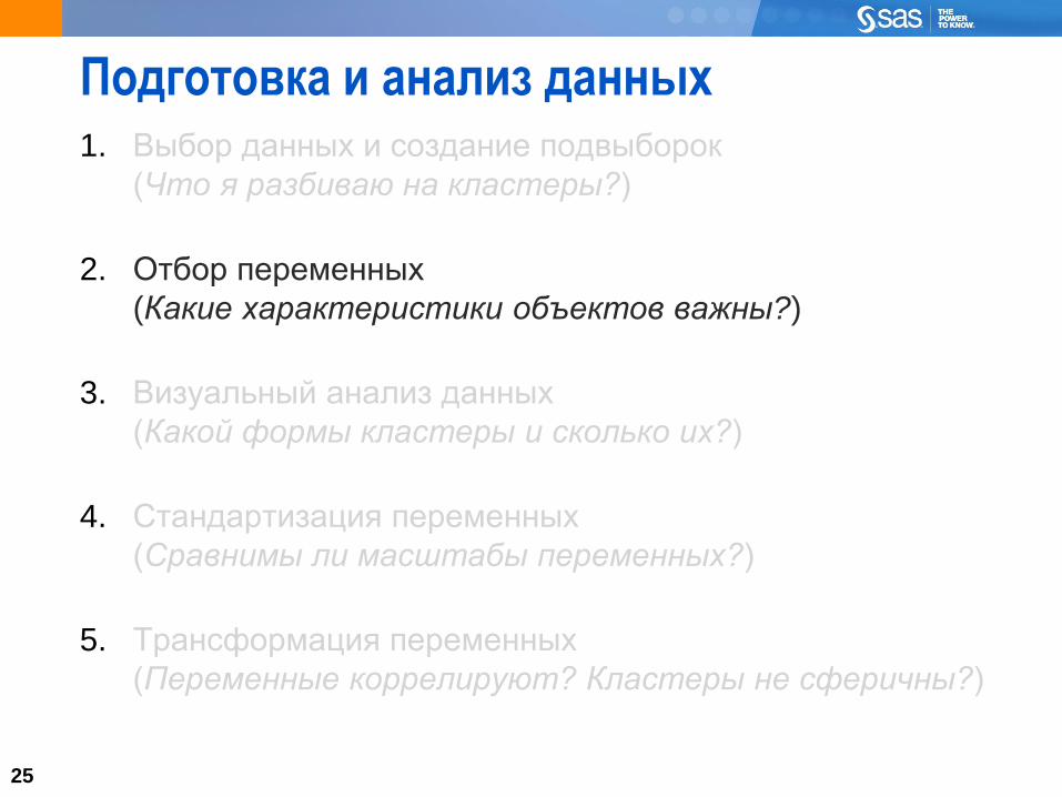
Подготовка и анализ данных1.
2. Отбор переменных
(Какие характеристики объектов важны?)
3.
4.
5.
25
26
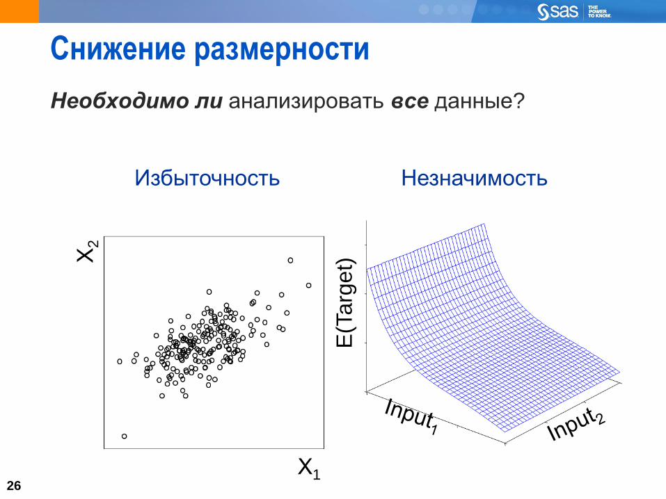
Снижение размерности
Необходимо ли анализировать все данные?Х
2
Х1
Избыточность
E(T
arg
et)
Незначимость
27
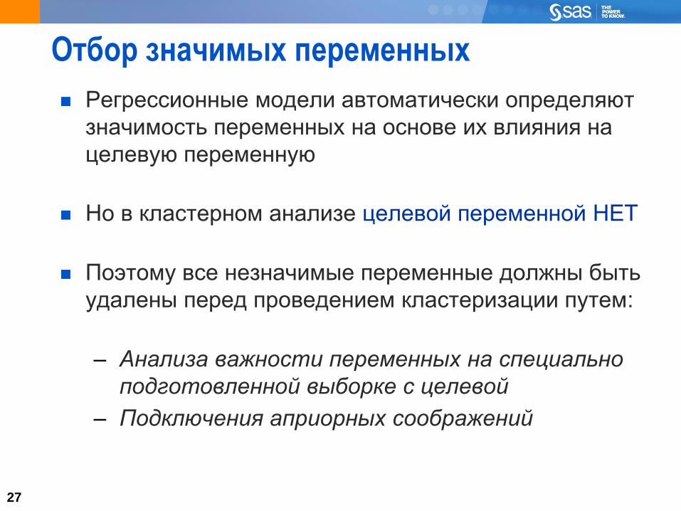
Отбор значимых переменных
Регрессионные модели автоматически определяют
значимость переменных на основе их влияния на
целевую переменную
Но в кластерном анализе целевой переменной НЕТ
Поэтому все незначимые переменные должны быть
удалены перед проведением кластеризации путем:
– Анализа важности переменных на специально
подготовленной выборке с целевой
– Подключения априорных соображений
27

28
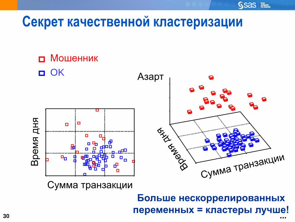
Секрет качественной кластеризации
OK
Мошенник
Сумма транзакции
...

29 ...
Секрет качественной кластеризации
OK
Мошенник
Сумма транзакции
30 ...
Секрет качественной кластеризации
OK
Мошенник
Сумма транзакции
Больше нескоррелированных
переменных = кластеры лучше!
Азарт

31
Удаление избыточных переменных
31
PROC VARCLUS DATA=SAS-data-set <options>;
BY variables;
VAR variables;
RUN;
PROC VARCLUS группирует избыточные переменные
Из каждой группы выбирается по одному
представителю, а остальные переменные удаляются,
тем самым снижая коллинеарность и число
переменных
32
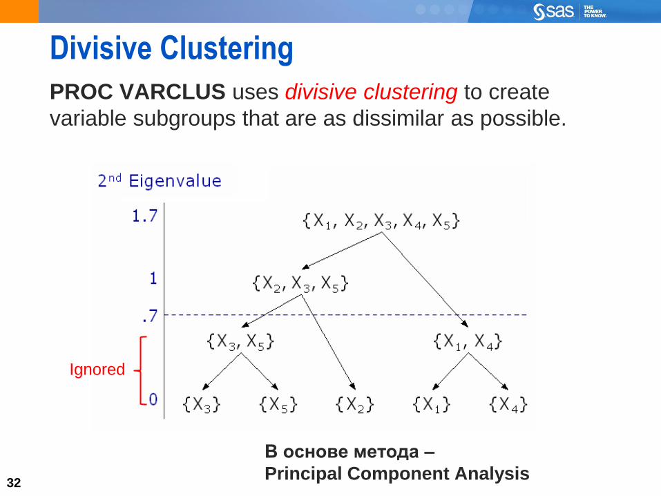
Divisive Clustering
PROC VARCLUS uses divisive clustering to create
variable subgroups that are as dissimilar as possible.
32
Ignored
В основе метода –
Principal Component Analysis

3333
clus02d01.sas
Ignored
Keep them

34
Подготовка и разведочный анализ
данных
Визуальный анализ

35
Подготовка и анализ данных1.
2.
3. Визуальный анализ данных
(Какой формы кластеры и сколько их?)
4.
5.
35
36
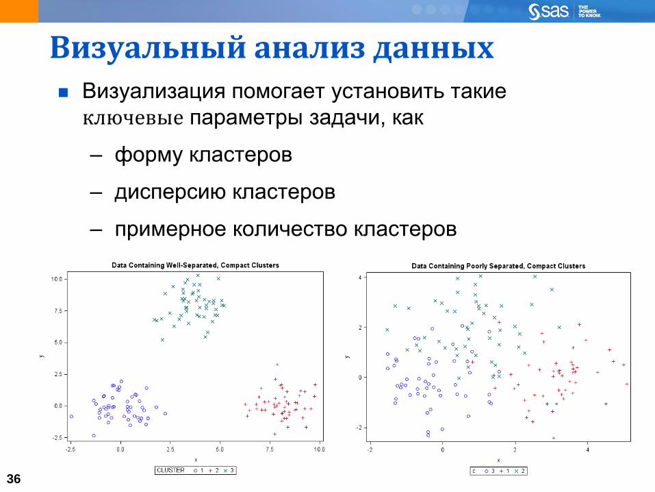
Визуальный анализ данных Визуализация помогает установить такие
ключевые параметры задачи, как
– форму кластеров
– дисперсию кластеров
– примерное количество кластеров

37
Principal Component Plots
x1
x2
Eigenvector 2
Eigenvector 1Eigenvalue 1
Eigenvalue 2
PROC PRINCOMP DATA=SAS-data-set <options>;
BY variables;
VAR variables;
RUN;

38
Multidimensional Scaling Plots
PROC MDS DATA=distance_matrix <options>;
VAR variables;
RUN;

39
Подготовка и разведочный анализ
данных
Стандартизация переменных

40
Подготовка и анализ данных1.
2.
3.
4. Стандартизация переменных
(Сравнимы ли масштабы переменных?)
5.
40
41
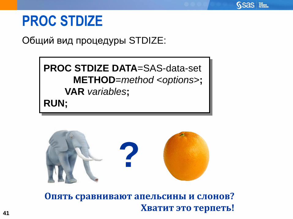
PROC STDIZE
Общий вид процедуры STDIZE:
41
PROC STDIZE DATA=SAS-data-set
METHOD=method <options>;
VAR variables;
RUN;
?Опять сравнивают апельсины и слонов?
Хватит это терпеть!
42
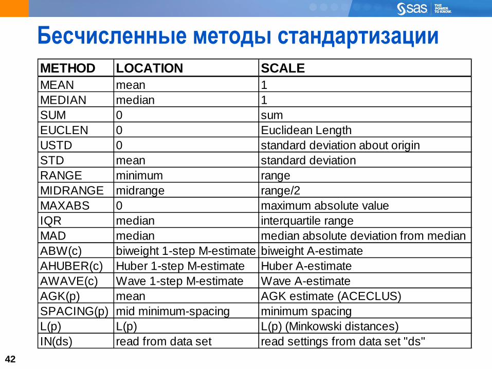
Бесчисленные методы стандартизации
42
METHOD LOCATION SCALE
MEAN mean 1
MEDIAN median 1
SUM 0 sum
EUCLEN 0 Euclidean Length
USTD 0 standard deviation about origin
STD mean standard deviation
RANGE minimum range
MIDRANGE midrange range/2
MAXABS 0 maximum absolute value
IQR median interquartile range
MAD median median absolute deviation from median
ABW(c) biweight 1-step M-estimate biweight A-estimate
AHUBER(c) Huber 1-step M-estimate Huber A-estimate
AWAVE(c) Wave 1-step M-estimate Wave A-estimate
AGK(p) mean AGK estimate (ACECLUS)
SPACING(p) mid minimum-spacing minimum spacing
L(p) L(p) L(p) (Minkowski distances)
IN(ds) read from data set read settings from data set "ds"
4343
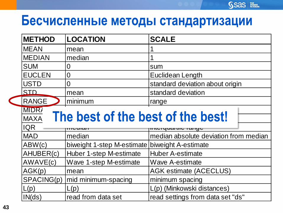
METHOD LOCATION SCALE
MEAN mean 1
MEDIAN median 1
SUM 0 sum
EUCLEN 0 Euclidean Length
USTD 0 standard deviation about origin
STD mean standard deviation
RANGE minimum range
MIDRANGE midrange range/2
MAXABS 0 maximum absolute value
IQR median interquartile range
MAD median median absolute deviation from median
ABW(c) biweight 1-step M-estimate biweight A-estimate
AHUBER(c) Huber 1-step M-estimate Huber A-estimate
AWAVE(c) Wave 1-step M-estimate Wave A-estimate
AGK(p) mean AGK estimate (ACECLUS)
SPACING(p) mid minimum-spacing minimum spacing
L(p) L(p) L(p) (Minkowski distances)
IN(ds) read from data set read settings from data set "ds"
Бесчисленные методы стандартизации
The best of the best of the best!

44
Подготовка и разведочный анализ
данных
Трансформация переменных
45
Подготовка и анализ данных1.
2.
3.
4.
5. Трансформация переменных
(Переменные коррелируют? Кластеры не сферичны?)
45
46
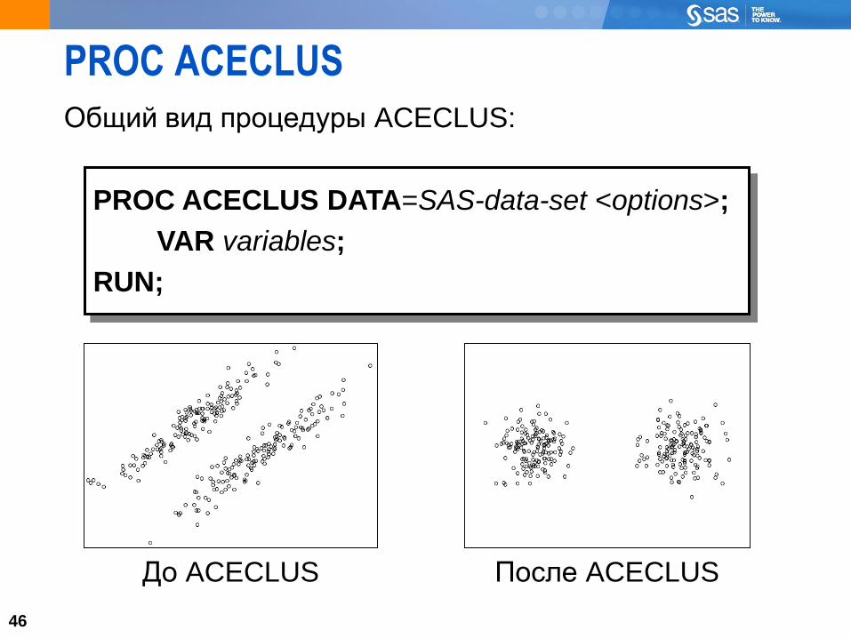
PROC ACECLUS
Общий вид процедуры ACECLUS:
46
PROC ACECLUS DATA=SAS-data-set <options>;
VAR variables;
RUN;
До ACECLUS После ACECLUS
47
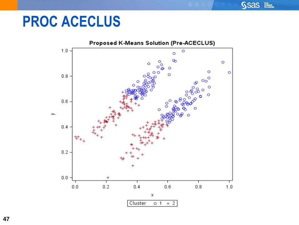
PROC ACECLUS
47

4848
PROC ACECLUS

49
Partitive Clustering
50
Partitive Clustering
Алгоритм К-Means

51
Partitive Clustering: optimization Кластеризация разделением оптимизирует
некоторую штрафную функцию, например:
– межкластерное расстояние
– внутрикластерную однородность (похожесть)
51
52
Оптимизирующие естественный критерий
группировки(K-means)
Параметрическое семейство алгоритмов
(Expectation-Maximization)
Непараметрическое семейство алгоритмов
(Kernel-based)
52
Семейства алгоритмов

53
Критерий естественной группировки
Поиск наилучшего разбиения множества объектов на
кластеры можно практически всегда можно свести к
оптимизации критерия естественной группировки:
– Максимизировать межкластерную сумму квадратов
расстояний, или
– Минимизировать внутрикластерную сумму
квадратов расстояний между объектами.
Большое межкластерное расстояние говорит о хорошей
разделенности кластеров
Малое внутрикластерное расстояние – признак
однородности объектов внутри группы
53
54
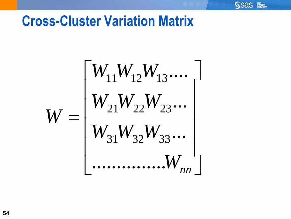
Cross-Cluster Variation Matrix
54
nnW
WWW
WWW
WWW
W
...............
...
...
....
333231
232221
131211

55
The Trace Function
Trace summarizes matrix W into a single number by adding
together its diagonal (variance) elements.
Simply adding matrix elements together makes trace very
efficient, but it also makes it scale dependent
Ignores the off-diagonal elements, so variables are treated
as if they were independent (uncorrelated).
Diminishes the impact of information from correlated variables.
55
+
-
56
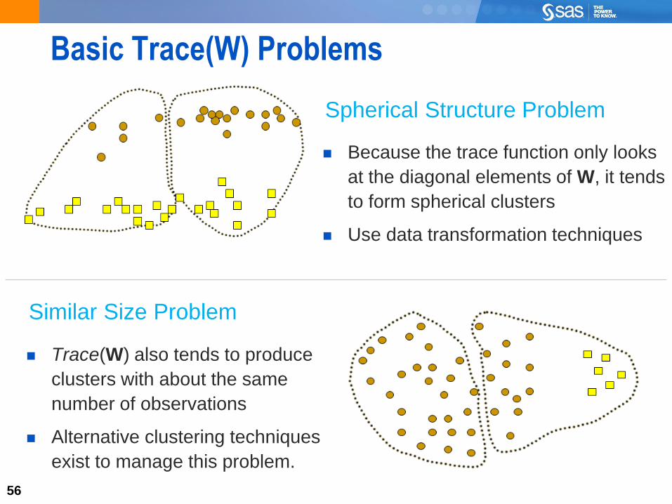
Basic Trace(W) Problems
Because the trace function only looks
at the diagonal elements of W, it tends
to form spherical clusters
Use data transformation techniques
56
Trace(W) also tends to produce
clusters with about the same
number of observations
Alternative clustering techniques
exist to manage this problem.
Spherical Structure Problem
Similar Size Problem
57
Partitive Clustering
Алгоритм К-MeansPROC FASTCLUS
58
The K-Means Methodology
The three-step k-means methodology:
1. Select (or specify) an initial set of cluster seeds
58
59
The K-Means Methodology
The three-step k-means methodology:
1.
2. Read the observations and update the seeds (known
after the update as reference vectors). Repeat until
convergence is attained
59
60
The K-Means Methodology
The three-step k-means methodology:
1.
2.
3. Make one final pass through the data, assigning
each observation to its nearest reference vector
60

61
k-Means Clustering Algorithm
1. Select inputs.
2. Select k cluster centers.
3. Assign cases to closest
center.
4. Update cluster centers.
5. Re-assign cases.
6. Repeat steps 4 and 5
until convergence.

62
k-Means Clustering Algorithm
1. Select inputs.
2. Select k cluster centers.
3. Assign cases to closest
center.
4. Update cluster centers.
5. Re-assign cases.
6. Repeat steps 4 and 5
until convergence.

63
k-Means Clustering Algorithm
1. Select inputs.
2. Select k cluster centers.
3. Assign cases to closest
center.
4. Update cluster centers.
5. Reassign cases.
6. Repeat steps 4 and 5
until convergence.
...

64
k-Means Clustering Algorithm
1. Select inputs.
2. Select k cluster centers.
3. Assign cases to closest
center.
4. Update cluster centers.
5. Reassign cases.
6. Repeat steps 4 and 5
until convergence.
...

65
k-Means Clustering Algorithm
1. Select inputs.
2. Select k cluster centers.
3. Assign cases to closest
center.
4. Update cluster centers.
5. Reassign cases.
6. Repeat steps 4 and 5
until convergence.
...
66
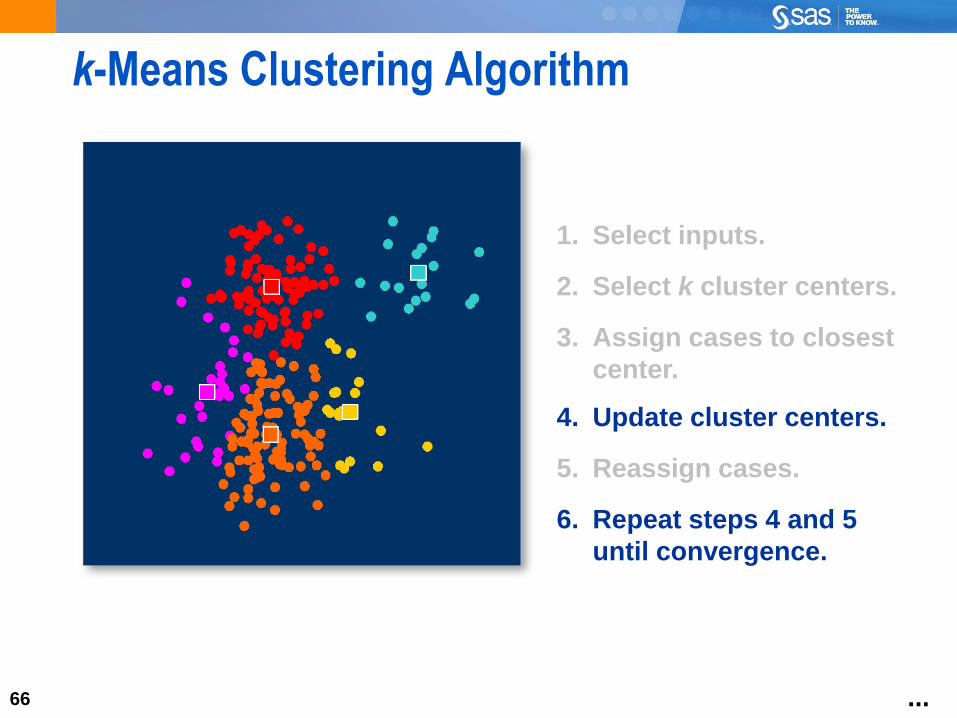
k-Means Clustering Algorithm
1. Select inputs.
2. Select k cluster centers.
3. Assign cases to closest
center.
4. Update cluster centers.
5. Reassign cases.
6. Repeat steps 4 and 5
until convergence.
...
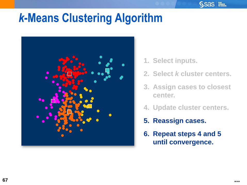
67
k-Means Clustering Algorithm
1. Select inputs.
2. Select k cluster centers.
3. Assign cases to closest
center.
4. Update cluster centers.
5. Reassign cases.
6. Repeat steps 4 and 5
until convergence.
...

68
k-Means Clustering Algorithm
1. Select inputs.
2. Select k cluster centers.
3. Assign cases to closest
center.
4. Update cluster centers.
5. Reassign cases.
6. Repeat steps 4 and 5
until convergence.
...

69
k-Means Clustering Algorithm
1. Select inputs.
2. Select k cluster centers.
3. Assign cases to closest
center.
4. Update cluster centers.
5. Reassign cases.
6. Repeat steps 4 and 5
until convergence.
...

70
k-Means Clustering Algorithm
1. Select inputs.
2. Select k cluster centers.
3. Assign cases to closest
center.
4. Update cluster centers.
5. Reassign cases.
6. Repeat steps 4 and 5
until convergence.
...

71
Segmentation Analysis
When no clusters exist,
use the k-means algorithm
to partition cases into
contiguous groups.

72
The FASTCLUS Procedure
General form of the FASTCLUS procedure:
Because PROC FASTCLUS produces relatively little
output, it is often a good idea to create an output data set,
and then use other procedures such as PROC MEANS,
PROC SGPLOT, PROC DISCRIM, or PROC CANDISC to
study the clusters.
72
PROC FASTCLUS DATA=SAS-data-set
<MAXC=>|<RADIUS=><options>;
VAR variables;
RUN;

73
The MAXITER= Option
The MAXITER= option sets the number of K-Means
iterations (the default number of iterations is 1)
73
X
XX
X
X
XX X
XX
XX
X
XX X
X
XX
X
XX XX
XX
X
… Time nTime 0 Time 1

74
The DRIFT Option
The DRIFT option adjusts the nearest reference vector as
each observation is assigned.
74
X
XX
X
X
XX X
XX
XX
X
X
XX X
X
XX
X
XX XX
X
…Time 0 Time 1 Time 2

75
The LEAST= Option
The LEAST = option provides the argument for the
Minkowski distance metric, changes the number of
iterations, and changes the convergence criterion.
75
Option Distance Max Iterations Converge=
default EUCLIDEAN 1 .02
LEAST=1 CITY BLOCK 20 .0001
LEAST=2 EUCLIDEAN 10 .0001

76
What Value of k to Use?
The number of seeds, k, typically translates to the final
number of clusters obtained. The choice of k can be made
using a variety of methods.
Subject-matter knowledge (There
are most likely five groups.)
Convenience (It is convenient to
market to three to four groups.)
Constraints (You have six products
and need six segments.)
Arbitrarily (Always pick 20.)
Based on the data (combined with
Ward’s method).

77
Problems with K-Means
Не всегда оптимальное
разбиение пространства
Плотность выборки?
Нет, не слышал!

78
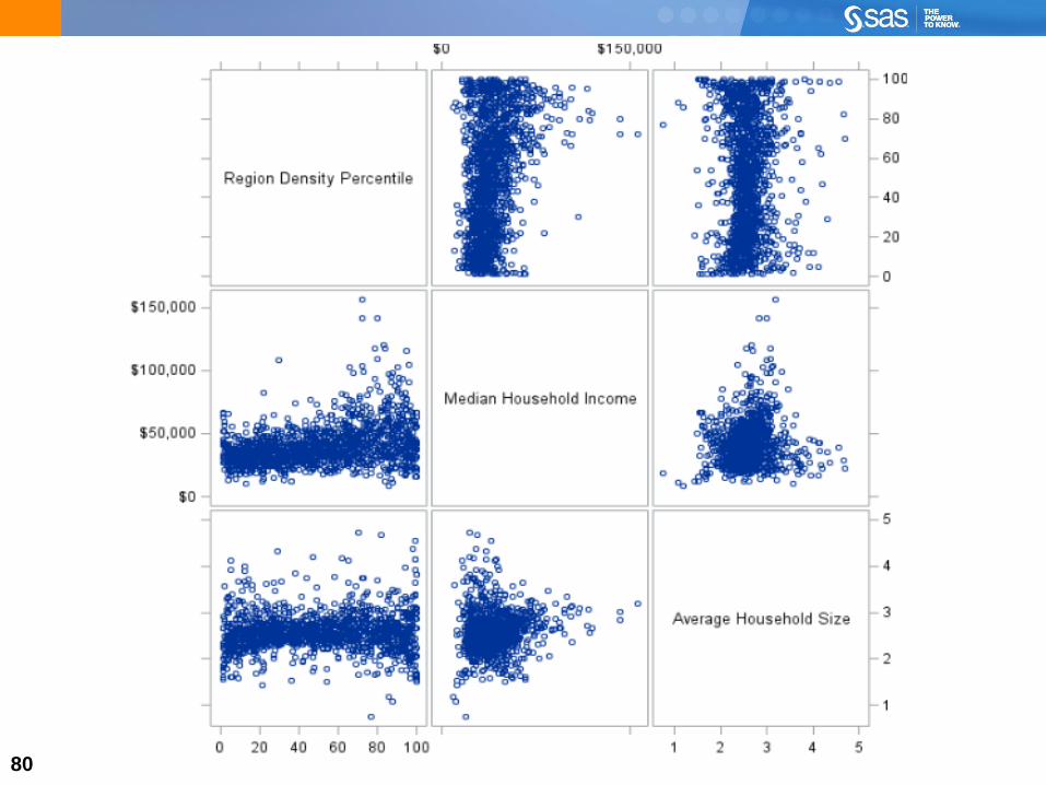
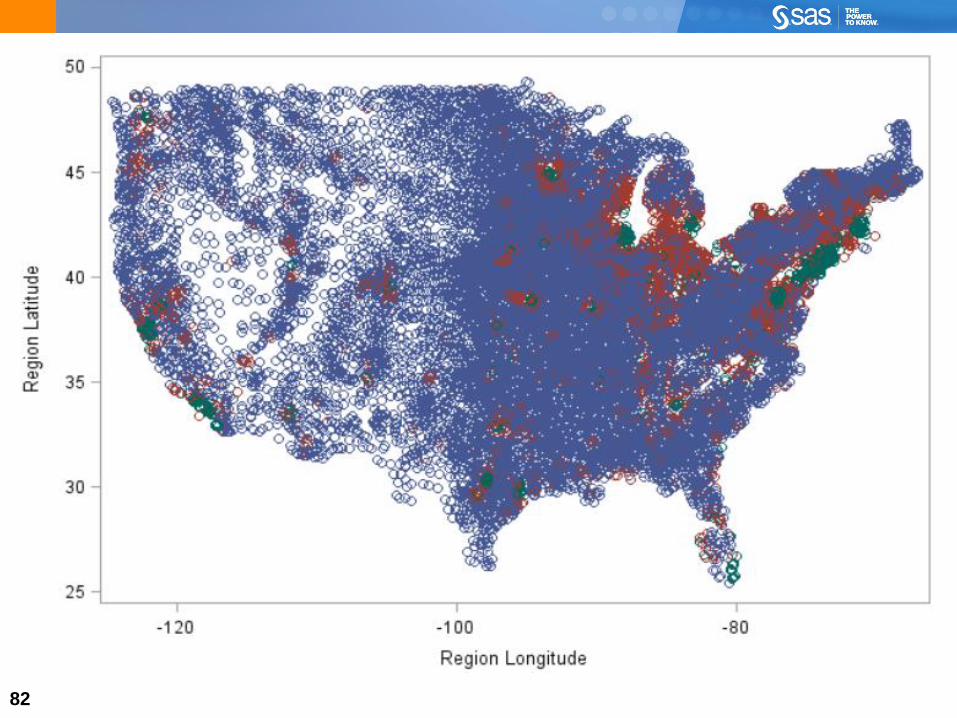
Grocery Store Case Study: Census Data
Analysis goal:
Where should you open new grocery store locations?
Group geographic regions based on income,
household size, and population density.
Explore the data.
Select the number of segments to create.
Create segments with a clustering
procedure.
Interpret the segments.
Map the segments.
Analysis plan:

79
K-Means Clustering for Segmentation
This demonstration illustrates the concepts
discussed previously.
79
8080

8181
8282
83
Partitive Clustering
Непараметрическая кластеризация

84
Parametric vs Non-Parametric Clustering
84
Параметрические алгоритмы плохи на density-based кластерах
Expectation-Maximization (+) Expectation-Maximization (-)
85
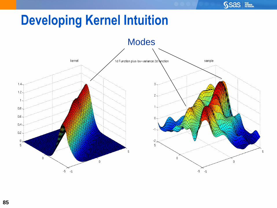
Developing Kernel Intuition
85
Modes
86
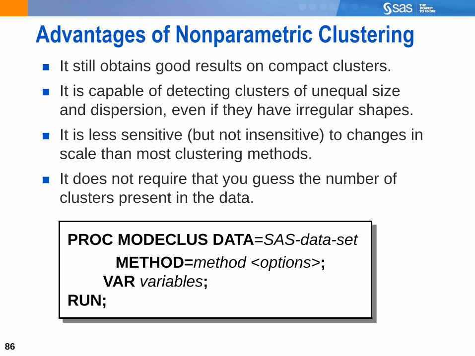
Advantages of Nonparametric Clustering
It still obtains good results on compact clusters.
It is capable of detecting clusters of unequal size
and dispersion, even if they have irregular shapes.
It is less sensitive (but not insensitive) to changes in
scale than most clustering methods.
It does not require that you guess the number of
clusters present in the data.
86
PROC MODECLUS DATA=SAS-data-set
METHOD=method <options>;
VAR variables;
RUN;

87
Significance Tests
If requested (the JOIN= option), PROC MODECLUS
can hierarchically join non-significant clusters.
Although a fixed-radius kernel (R=) must be specified,
the choice of smoothing parameter is not critical.
87
88
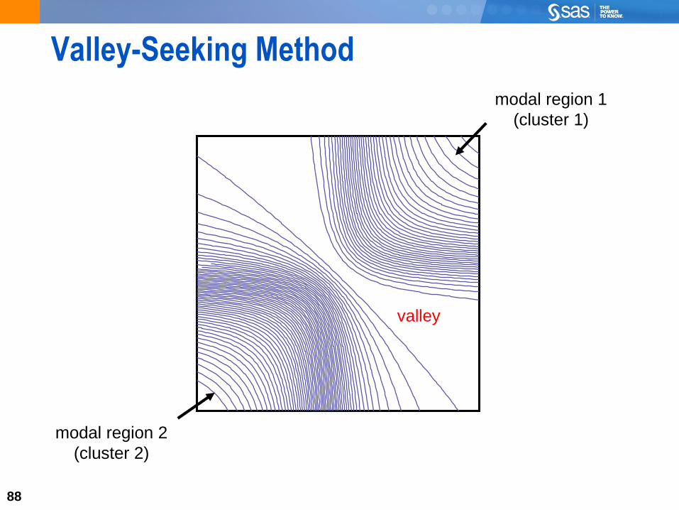
Valley-Seeking Method
88
valley
modal region 1
(cluster 1)
modal region 2
(cluster 2)
89
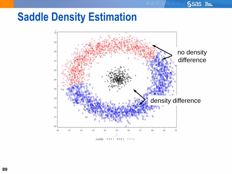
Saddle Density Estimation
89
no density
difference
density difference
90
Hierarchically Joining Non-Significant Clusters
This demonstration illustrates the concepts
discussed previously.
90

9191

9292

93
Иерархическаякластеризация

94
Hierarchical Clustering
94
95
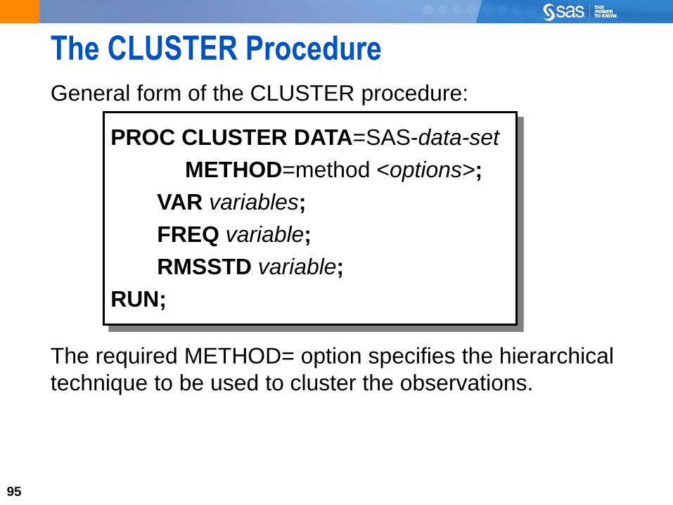
The CLUSTER Procedure
General form of the CLUSTER procedure:
The required METHOD= option specifies the hierarchical
technique to be used to cluster the observations.
95
PROC CLUSTER DATA=SAS-data-set
METHOD=method <options>;
VAR variables;
FREQ variable;
RMSSTD variable;
RUN;

96
Cluster and Data Types
96
Hierarchical MethodDistance Data
Required?
Average Linkage Yes
Two-Stage Linkage Some Options
Ward’s Method Yes
Centroid Linkage Yes
Complete Linkage Yes
Density Linkage Some Options
EML No
Flexible-Beta Method Yes
McQuitty’s Similarity Yes
Median Linkage Yes
Single Linkage Yes

97
The TREE Procedure
General form of the TREE procedure:
The TREE procedure either
displays the dendrogram (LEVEL= option), or
assigns the observations to a specified number
of clusters (NCLUSTERS= option).
97
PROC TREE DATA=<dendrogram> <options>;
RUN;

98
Иерархическаякластеризация
Параметры алгоритма

99
Average Linkage
The distance between clusters is the average distance
between pairs of observations.
99
K LCi Cj
ji
LK
KL xxdnn
D
, 1
CKd(xi, xj)
CL

100
Two-Stage Density Linkage
A nonparametric density estimate is used to determine
distances, and recover irregularly shaped clusters.
100
2. Apply single linkage
modal cluster K
modal cluster L
modal cluster K
modal cluster L
DKL
1. Form ‘modal’ clusters
101
The Two Stages of Two-stage
The first stage, known as density linkage, constructs a
distance measure, d*, based on kernel density
estimates and creates modal clusters.
The second stage ensures that a cluster has at least
“n” members before it can be fused. Clusters are fused
using single linkage (joins based on the nearest points
between two clusters).
The measure d* can be based on three methods. This
course uses the k-nearest neighbor method.
101
102
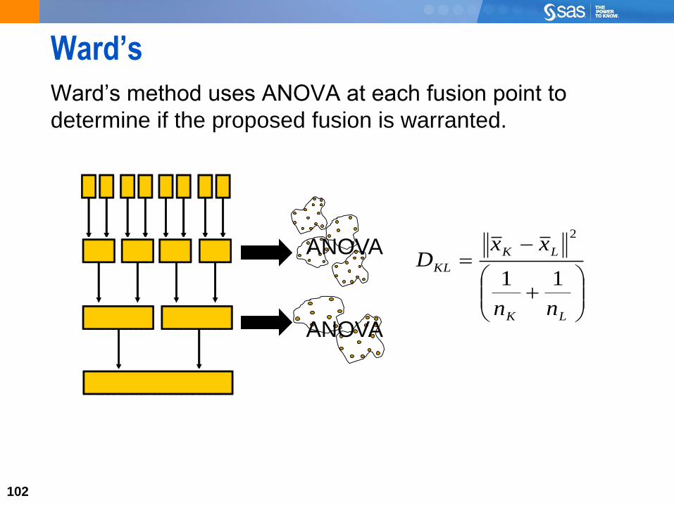
Ward’s
Ward’s method uses ANOVA at each fusion point to
determine if the proposed fusion is warranted.
102
LK
LK
KL
nn
xxD
11
2
ANOVA
ANOVA

103
Additional Clustering Methods
Centroid Linkage
Complete Linkage
Density Linkage
Single Linkage
103
X
XCK
CL
CK
CL
CK
CLCK
CL

104
Centroid Linkage
The distance between clusters is the squared Euclidean
distance between cluster centroids and .
104
KxLx
2
LKKLD xx
X
XDKL
CK
CL
105
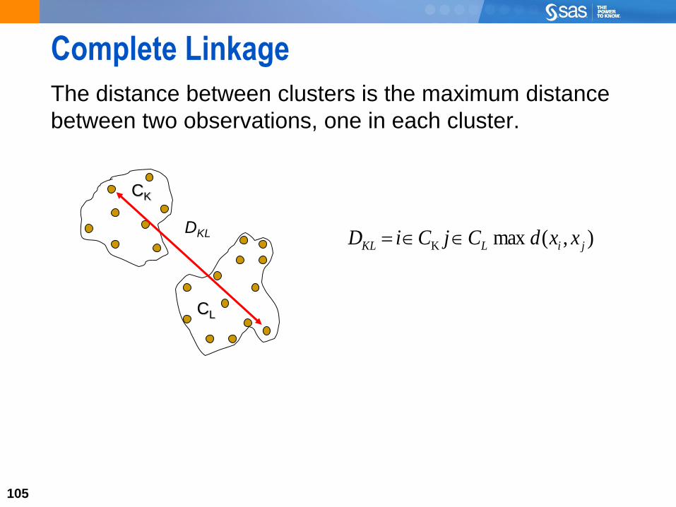
Complete Linkage
The distance between clusters is the maximum distance
between two observations, one in each cluster.
105
),(max K jiLKL xxdCjCiD DKL
CK
CL

106
Density Linkage
1. Calculate a new distance metric, d*, using k-nearest
neighbor, uniform kernel, or Wong’s hybrid method.
2. Perform single linkage clustering with d*.
106
)(
1
)(
1
2
1,*
ji
jixfxf
xxdd*(xi,xj)
CK
CL
107
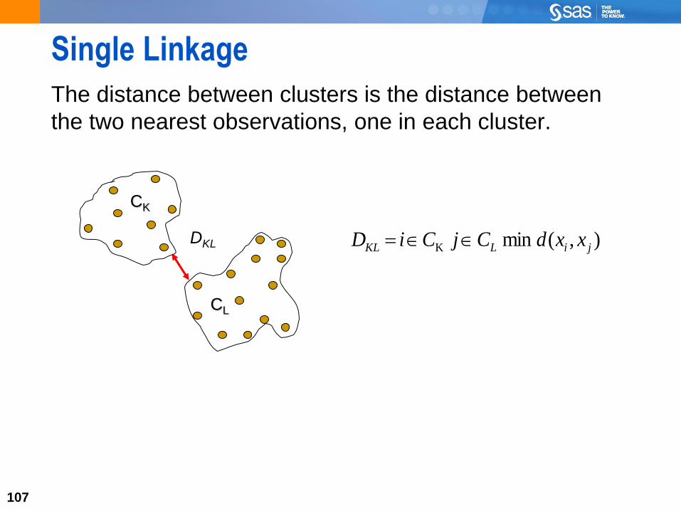
Single Linkage
The distance between clusters is the distance between
the two nearest observations, one in each cluster.
107
),(min K jiLKL xxdCjCiD DKL
CK
CL

108
Оценка результатов кластеризации
Оптимальное количество кластеров
109
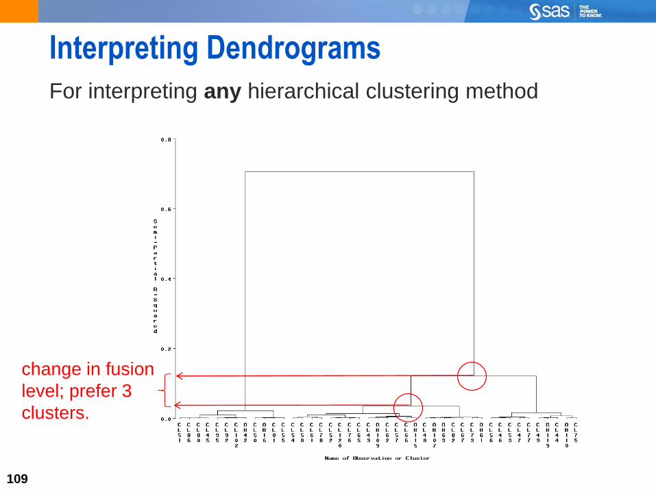
Interpreting Dendrograms
For interpreting any hierarchical clustering method
change in fusion
level; prefer 3
clusters.
110
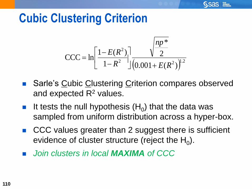
Cubic Clustering Criterion
Sarle’s Cubic Clustering Criterion compares observed
and expected R2 values.
It tests the null hypothesis (H0) that the data was
sampled from uniform distribution across a hyper-box.
CCC values greater than 2 suggest there is sufficient
evidence of cluster structure (reject the H0).
Join clusters in local MAXIMA of CCC
2.122
2
)(001.0
2
*
1
)(1lnCCC
RE
np
R
RE

111
Other Useful Statistics
Pseudo-F Statistics
Pseudo-T2 Statistics
/( 1)PSF
/( )
g
n g
B
W
PST2
( 2)
m k l
k l k ln n
W W W
W W
Join clusters
if T2 statistics is in local
MINIMUM
Join clusters
if statistics is in local
MAXIMUM

112
Interpreting PSF and PST2
candidates
candidates
Read in this
Direction
Pseudo-F Statistics
Pseudo-T2 Statistics

113
Оценка результатов кластеризации
Профилирование кластеров
114
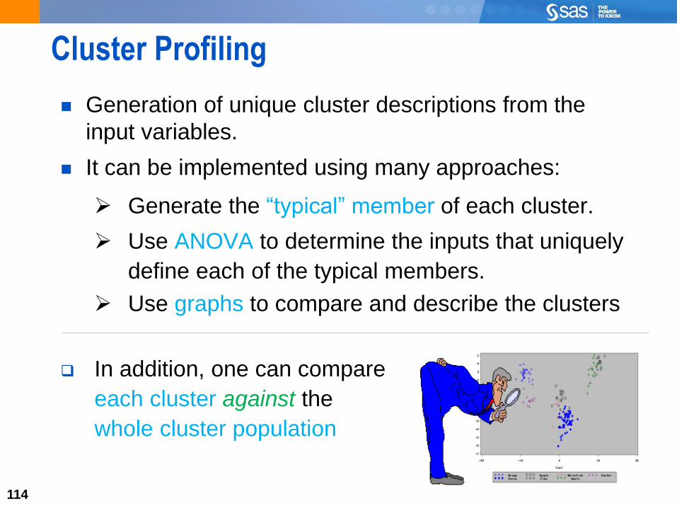
Cluster Profiling
Generation of unique cluster descriptions from the
input variables.
It can be implemented using many approaches:
Generate the “typical” member of each cluster.
Use ANOVA to determine the inputs that uniquely
define each of the typical members.
Use graphs to compare and describe the clusters
In addition, one can compare
each cluster against the
whole cluster population
115
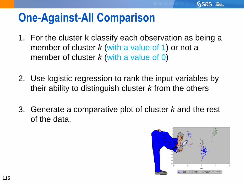
One-Against-All Comparison
1. For the cluster k classify each observation as being a
member of cluster k (with a value of 1) or not a
member of cluster k (with a value of 0)
2. Use logistic regression to rank the input variables by
their ability to distinguish cluster k from the others
3. Generate a comparative plot of cluster k and the rest
of the data.

116
Оценка результатов кластеризации
Применение модели кластеризации к новым
наблюдениям
117
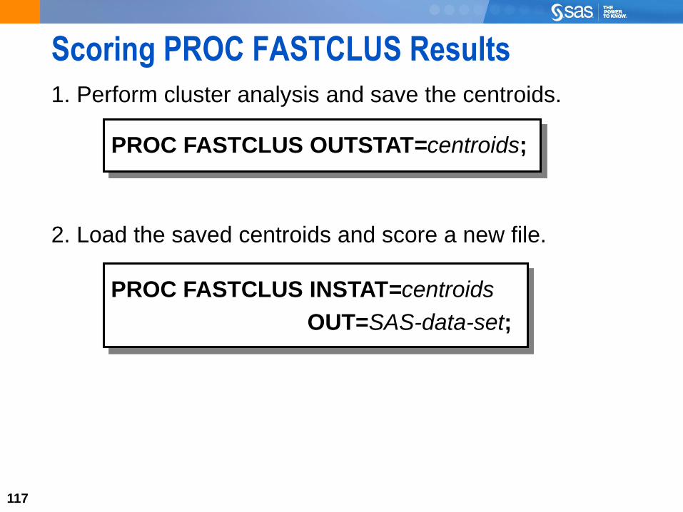
Scoring PROC FASTCLUS Results
1. Perform cluster analysis and save the centroids.
2. Load the saved centroids and score a new file.
PROC FASTCLUS OUTSTAT=centroids;
PROC FASTCLUS INSTAT=centroids
OUT=SAS-data-set;

118
Scoring PROC CLUSTER Results
1. Perform the hierarchical cluster analysis.
2. Generate the cluster assignments.
PROC CLUSTER METHOD= OUTTREE=tree;
VAR variables;
RUN;
PROC TREE DATA=tree N=nclusters OUT=treeout;
RUN;
continued...
119
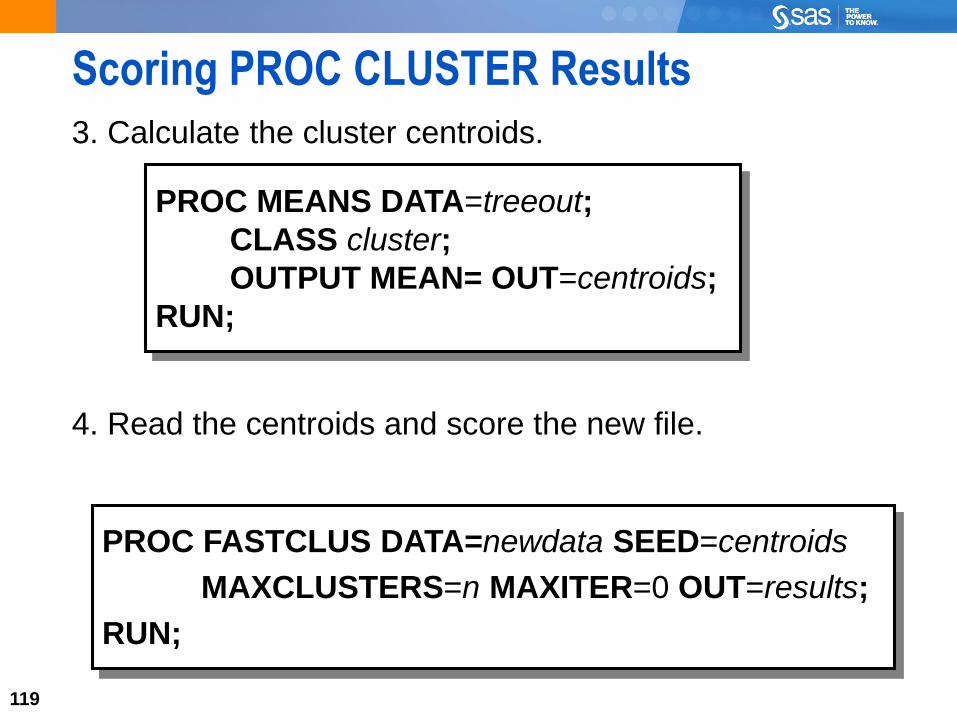
Scoring PROC CLUSTER Results
3. Calculate the cluster centroids.
4. Read the centroids and score the new file.
PROC MEANS DATA=treeout;
CLASS cluster;
OUTPUT MEAN= OUT=centroids;
RUN;
PROC FASTCLUS DATA=newdata SEED=centroids
MAXCLUSTERS=n MAXITER=0 OUT=results;
RUN;

120
Кейс
Happy Household Study

121
The Happy Household Catalog
A retail catalog company with a strong online presence
monitors quarterly purchasing behavior for its customers,
including sales figures summarized across departments
and quarterly totals for 5.5 years of sales.
HH wants to improve customer relations by
tailoring promotions to customers based on
their preferred type of shopping experience
Customer preferences are difficult to ascertain
based solely on opportunistic data.
122
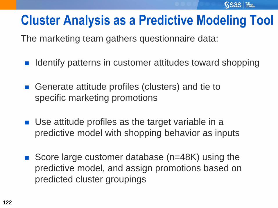
Cluster Analysis as a Predictive Modeling Tool
The marketing team gathers questionnaire data:
Identify patterns in customer attitudes toward shopping
Generate attitude profiles (clusters) and tie to
specific marketing promotions
Use attitude profiles as the target variable in a
predictive model with shopping behavior as inputs
Score large customer database (n=48K) using the
predictive model, and assign promotions based on
predicted cluster groupings

123
Preparation for Clustering
1. Data and Sample Selection
2. Variable Selection (What characteristics matter?)
3. Graphical Exploration (What shape/how many
clusters?)
4. Variable Standardization (Are variable scales
comparable?)
5. Variable Transformation (Are variables correlated?
Are clusters elongated?)

124
Data and Sample Selection
A study is conducted to identify patterns in customer
attitudes toward shopping
Online customers are asked to complete a questionnaire
during a visit to the company’s retail Web site. A sample
of 200 complete data questionnaires is analyzed.

125
Preparation for Clustering
1. Data and Sample Selection (Who am I clustering?)
2. Variable Selection
3. Graphical Exploration (What shape/how many
clusters?)
4. Variable Standardization (Are variable scales
comparable?)
5. Variable Transformation (Are variables correlated?
Are clusters elongated?)
126
Variable Selection
This demonstration illustrates the concepts
discussed previously.
clus06d01.sas
127
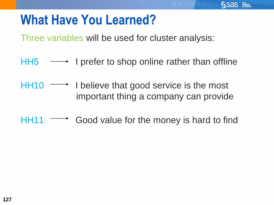
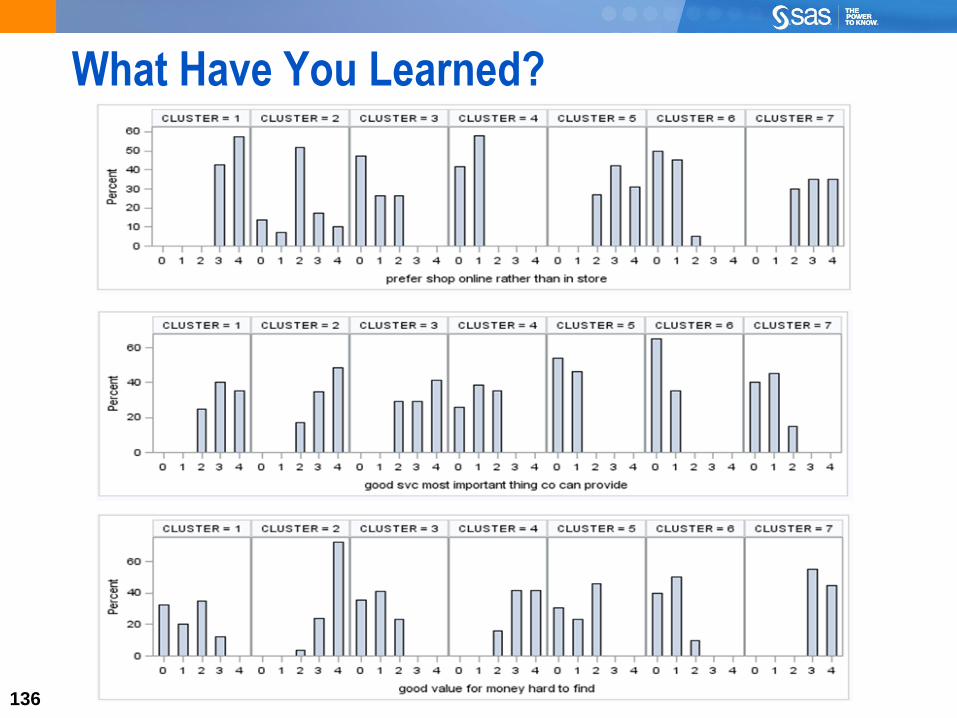
What Have You Learned?
Three variables will be used for cluster analysis:
HH5 I prefer to shop online rather than offline
HH10 I believe that good service is the most
important thing a company can provide
HH11 Good value for the money is hard to find

128
Preparation for Clustering
1. Data and Sample Selection (Who am I clustering?)
2. Variable Selection (What characteristics matter?)
3. Graphical Exploration
4. Variable Standardization (Are variable scales
comparable?)
5. Variable Transformation (Are variables correlated?
Are clusters elongated?)
129
Graphical Exploration of Selected Variables
This demonstration illustrates the concepts
discussed previously.
clus06d02.sas

130
Preparation for Clustering
1. Data and Sample Selection (Who am I clustering?)
2. Variable Selection (What characteristics matter?)
3. Graphical Exploration (What shape/how many
clusters?)
4. Variable Standardization
5. Variable Transformation

131
What Have You Learned?
Standardization is unnecessary in this example
because all variables are on the same scale of
measurement
Transformation might be unnecessary in this example
because there is not evidence of elongated cluster
structure from the plots, and the variables have low
correlation.

132
Selecting a Clustering Method
With 200 observations, it is a good idea to use a
hierarchical clustering technique.
Ward’s method is selected for ease of interpretation
Select number of clusters with CCC, PSF and PST2
Use cluster plots to assist in providing cluster labels
133
Hierarchical Clustering and Determining the Number of Clusters
This demonstration illustrates the concepts
discussed previously.
clus06d03.sas
134
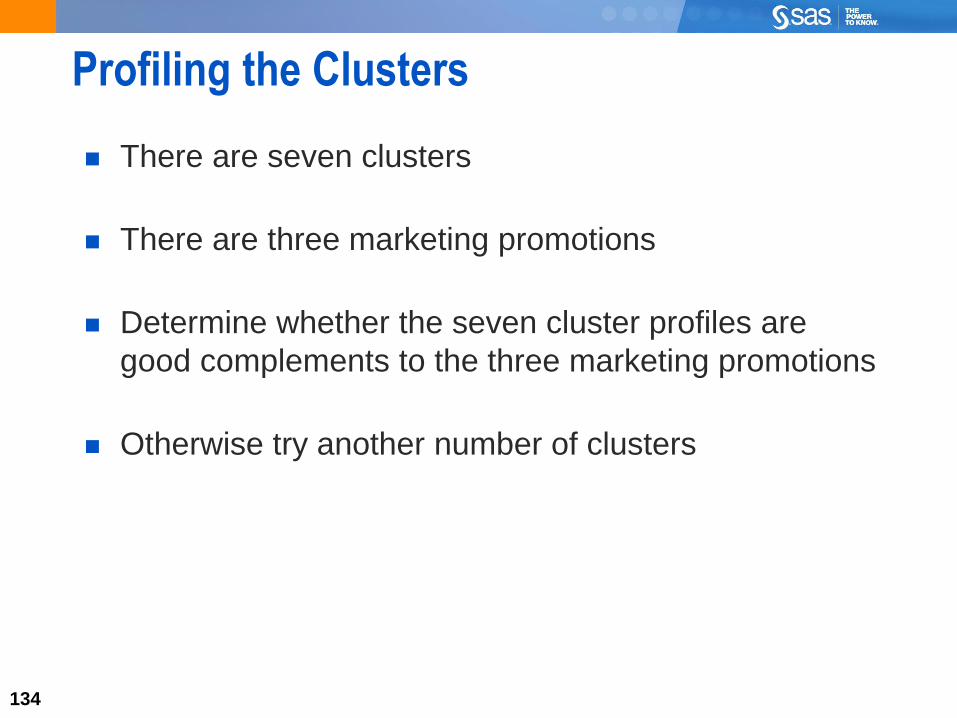
Profiling the Clusters
There are seven clusters
There are three marketing promotions
Determine whether the seven cluster profiles are
good complements to the three marketing promotions
Otherwise try another number of clusters
135
Profiling the Seven-Cluster Solution
This demonstration illustrates the concepts
discussed previously.
clus06d04.sas
136
What Have You Learned?

137
What Have You Learned?
138
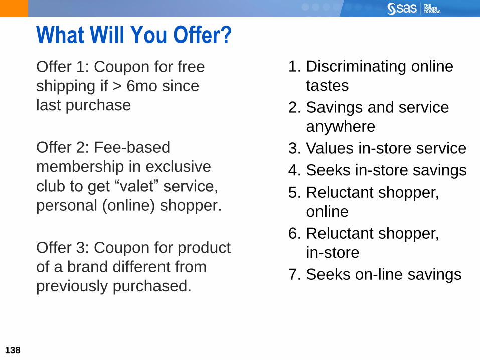
What Will You Offer?
Offer 1: Coupon for free
shipping if > 6mo since
last purchase
Offer 2: Fee-based
membership in exclusive
club to get “valet” service,
personal (online) shopper.
Offer 3: Coupon for product
of a brand different from
previously purchased.
1. Discriminating online
tastes
2. Savings and service
anywhere
3. Values in-store service
4. Seeks in-store savings
5. Reluctant shopper,
online
6. Reluctant shopper,
in-store
7. Seeks on-line savings

139
What Will You Offer?
Offer 1: Coupon for free
shipping if > 6mo since
last purchase
Offer 2: Fee-based
membership in exclusive
club to get “valet” service,
personal (online) shopper.
Offer 3: Coupon for product
of a brand different from
previously purchased.
1. Discriminating online
tastes
2. Savings and service
anywhere
3. Values in-store service
4. Seeks in-store savings
5. Reluctant shopper,
online
6. Reluctant shopper,
in-store
7. Seeks on-line savings
Offer will be made based on cluster classification
and a high customer lifetime value score.

140
Predictive ModelingThe marketing team can choose from a variety of predictive
modeling tools, including logistic regression, decision trees,
neural networks, and discriminant analysis
Logistic regression and NN should be neglected because of
the small sample and large number of input variables
Discriminant analysis is used in this example
PROC DISCRIM DATA=data-set-1;
<PRIORS priors-specification;>
CLASS cluster-variable;
VAR input-variables;
RUN;
141
Modeling Cluster Membership
This demonstration illustrates the concepts
discussed previously.
clus0605.sas

142
Scoring the Database
Once a model has been developed to predict cluster
membership from purchasing data, the full customer
database can be scored.
Customers are offered specific promotions based on
predicted cluster membership.
PROC DISCRIM DATA=data-set-1
TESTDATA=data-set-2 TESTOUT=scored-data;
PRIORS priors-specification;
CLASS cluster-variable;
VAR input-variables;
RUN;

143
Let’s Cluster the World!