rec1p1ent s fhw affx-95/1333-lf
TRANSCRIPT

Technical Report Documentation Page
l. Report No. . Rec1p1ent s
FHW AffX-95/1333-lF 4. T1 e an u ti e 5. Report ate
RECYCLING CRUMB RUBBER MODIFIED ASPHALT PAVEMENTS
May 1995 Revised: July 1995
gan1Zati0n Co e
William W. Crockford, Danai Makunike, Richard R. Davison, Tom Scullion, and Travis C. Billiter
ormmg aniZation ame an
Texas Transportation Institute The Texas A&M University System College Station, Texas 77843-3135 1 . ponsormg Agency ame an Address
Texas Department of Transportation Research and Technology Transfer Office P. 0. Box 5080 Austin, Texas 78763-5080
15. Supp ementary Notes
11.
Study No. 0-1333
Research performed in cooperation with the Texas Department of Transportation and the U.S. Department of Transportation, Federal Highway Administration. Research Study Title: Recycling Second Generation Asphalt Rubber Pavements
There has been concern that the legislative mandate to use waste rubber in paving applications will result in a severe environmental problem when it becomes necessary to recycle these pavements. If successful recycling is possible, the long term performance of these pavements becomes a concern. The results of this study indicate that it is possible to recycle this material. However, some techniques for conventional asphalt mixture design, material processing, and construction must be modified to ensure this success, and some techniques may not be appropriate when waste rubber is present in the mixture to be recycled. Many of the results presented in this study are based on experiences in Tyler and San Antonio, Texas, where two of the earliest crumb rubber recycling operations in the United States have transpired.
17. Key or
Crwnb Rubber, Asphalt, Pavements
.7 (8-72)
18. Distri ution tatement
No Restrictions. This docwnent is available to the public through NTIS: National Technical Information Service 5285 Port Royal Road Springfield, Virginia 22161
. nee
Reproduction of completed page authorized


RECYCLING CRUMB RUBBER MODIFIED ASPHALT PAVEMENTS
by
William W. Crockford Danai Makunike
Richard R. Davison Tom Scullion
and Travis C. Billiter
Research Report 1333-lF Research Study Number 0-1333
Research Study Title: Recycling Second Generation Asphalt Rubber Pavements
Sponsored by the Texas Department of Transportation
In Cooperation with U.S. Department of Transportation,
Federal Highway Administration
May 1995 Revised: July 1995
TEXAS TRANSPORTATION INSTITUTE The Texas A&M University System College Station, Texas 77843-3135


IMPLEMENTATION STATEMENT
Study results provide the department with evidence that plant recycling of crumb
rubber modified asphalt pavements is possible with RAP contents up to 30 percent. These
results are based on a recycling project in the San Antonio District on Interstate 10. The
recycle was required because of a premature failure of a crumb rubber modified overlay.
The continued good performance of the materials placed in the last portion of the original
overlay indicates that the design philosophy used for the recycle operation could improve
virgin CRM materi_al as well. These sections were designed using a coarse matrix, high
binder concept, and they are still performing well.
v

DISCLAIMER
The contents of this report reflect the views of the authors who are responsible for the
opinions, findings, and conclusions presented herein. The contents do not necessarily reflect
the official views or policies of the Texas Department of Transportation or the Federal
Highway Administration (FHW A). This report does not constitute a standard, specification,
or regulation, nor is it intended for construction, bidding, or permit purposes.
No warranty is made by the Texas Department of Transportation, the Federal Highway
Administration, the Texas Transportation Institute, or the authors as to the accuracy,
completeness, reliability, usability, or suitability of testing equipment and its associated data
and docwnentation. No responsibility is asswned by the above parties for incorrect results
or damages resulting from use of the equipment.
The engineer in charge of the study was William W. Crockford, PhD, P.E. #67547.
vu
ACKNOWLEDGMENT
TTI appreciates the support given by TxDOT and FHW A during the course of this
study. Mike Coward, Earl Leaverton, and Patrick Downey of TxDOT provided valuable
assistance in the field and provided summaries of field and plant measurements. The air
quality and leachate tests were conducted by Southwestern Laboratories. David Kight of
TxDOT (retired) provided invaluable assistance on mix design issues.
Vlll

TABLE OF CONTENTS
LIST OF FIGURES ............................................. XI
LIST OF TABLES . . . . . . . . . . . . . . . . . . . . . . . . . . . . . . . . . . . . . . . . . . . . xiv
ABBREVIATIONS . . . . . .. . . . . . . . . . . . . . . . . . . . . . . . . . . . . . . . . . . . . . . . xvi
SUMMARY . . . . . . . . . . . . . . . . . . . . . . . . . . . . . . . . . . . . . . . . . . . . . . . . xvii
I. INTRODUCTION . . . . . . . . . . . . . . . . . . . . . . . . . . . . . . . . . . . . . . . . . . . 1
LITERATURE REVIEW . . . . . . . . . . . . . . . . . . . . . . . . . . . . . . . . . . . . . 3
LEGISLATIVE MANDATE FOR USE OF WASTE TIRE RUBBER . . . . . . 11
SURVEY OF STATES' EXPERIENCE WITH CRM PAVEMENTS ....... 13
OVERVIEW OF SEQUENCE OF CONSTRUCTION . . . . . . . . . . . . . . . . . 18
IL PROCESS AND MATERIALS EVALUATION . . . . . . . . . . . . . . . . . . . . . . 23
ENVIRONMENT AL ISSUES . . . . . . . . . . . . . . . . . . . . . . . . . . . . . . . . . 23
PERFORMANCE RELATED CHARACTERISTICS . . . . . . . . . . . . . . . . . 26
BINDER CHARACTERISTICS . . . . . . . . . . . . . . . . . . . . . . . . . . . . . . . . 42
III. CONCLUSIONS . . . . . . . . . . . . . . . . . . . . . . . . . . . . . . . . . . . . . . . . . . . 55
ENVIRONMENT AL . . . . . . . . . . . . . . . . . . . . . . . . . . . . . . . . . . . . . . . 55
DESIGN AND CONSTRUCTION PRACTICE . . . . . . . . . . . . . . . . . . . . . 55
PERFORMANCE . . . . . . . . . . . . . . . . . . . . . . . . . . . . . . . . . . . . . . . . . 56
PERMEABILITY . . . . . . . . . . . . . . . . . . . . . . . . . . . . . . . . . . . . . . . . . . 57
BINDER PROPERTIES . . . . . . . . . . . . . . . . . . . . . . . . . . . . . . . . . . . . . 57
IV. RECOMMENDATIONS . . . . . . . . . . . . . . . . . . . . . . . . . . . . . . . . . . . . . . 59
ENVIRONMENT AL . . . . . . . . . . . . . . . . . . . . . . . . . . . . . . . . . . . . . . . 59
PERFORMANCE . . . . . . . . . . . . . . . . . . . . . . . . . . . . . . . . . . . . . . . . . 59
PERMEABILITY . . . . . . . . . . . . . . . . . . . . . . . . . . . . . . . . . . . . . . . . . . 59
DESIGN AND CONSTRUCTION . . . . . . . . . . . . . . . . . . . . . . . . . . . . . . 60
V. REFERENCES . . . . . . . . . . . . . . . . . . . . . . . . . . . . . . . . . . . . . . . . . . . . . 63
APPENDIX A - TEST PROCEDURES USED IN THIS STUDY ............ A-1
CORPS OF ENGINEERS GYRATORY TEST ..................... A-1
IX

WATER PERMEABILITY OF CRM ASPHALT :MIXTURES .......... A-4
METHOD I: DETERMINATION OF THE PERMEABILITY OF CRUMB
RUBBER MODIFIED ASPHALT (Constant Head) . . . . . . . . . . . . . . . . . . A-5
METHOD II: FALLING HEAD TEST PROCEDURE
(for mixtures with greater than 3% air voids) ...................... A-12
PRINCIPLES OF GROUND PENETRATING RADAR ............... A-15
APPENDIX B - CONSTRUCTION MONITORING DATA ................. B-1
SAN ANTONIO PAVEMENTS ................................ B-1
ENVIRONMENTAL MONITORING ............................ B-8
PERFORMANCE . . . . . . . . . . . . . . . . . . . . . . . . . . . . . . . . . . . . . . . . B-11
LABORATORY STUDIES .................................. B-13
FIELD STUDIES ......................................... B-34
APPENDIX C - ASPHALT RUBBER RECYCLING GUIDELINES ........... C-1
CONSTRUCTION ALTERNATIVES ............................ C-1
STORAGE AND HANDLING OF CRM .......................... C-3
HOT :MIX EQUIPMENT AND PRODUCTION ..................... C-4
PAVING EQUIPMENT ..................................... C-4
OTHER CONSTRUCTION GUIDELINES ........................ C-5
LAYDOWN AND COMPACTION ............................. C-6
RELATED PUBLICATIONS .................................. C-7
SCOPE ................................................. C-8
EVALUATE RAP ........................................ C-10
EVALUATE VIRGIN MATERIAL ............................ C-12
DESIGN NEW BLEND .................................... C-12
APPENDIX D - ALTERNATIVE USES OF RECYCLED RUBBER . . . . . . . . . . D-1
ENERGY CONVERSION ...... ·. . . . . . . . . . . . . . . . . . . . . . . . . . . . . D-1
WHOLE TIRE APPLICATIONS . . . . . . . . . . . . . . . . . . . . . . . . . . . . . . D-1
SHREDDED RUBBER APPLICATIONS . . . . . . . . . . . . . . . . . . . . . . . . D-2
x

Figure 1.
Figure 2.
Figure 3.
Figure 4.
Figure 5.
Figure 6.
Figure 7.
Figure 8.
Figure 9.
Figure 10.
Figure 11.
Figure 12.
Figure 13.
Figure 14.
Figure 15.
Figure 16.
Figure 17.
Figure 18.
LIST OF FIGURES
Page
IH-10 Recent Traffic Growth . . . . . . . . . . . . . . . . . . . . . . . . . 18
IH-10 Daily Traffic Counts . . . . . . . . . . . . . . . . . . . . . . . . . . . 19
IH-10 Monthly Traffic Counts . . . . . . . . . . . . . . . . . . . . . . . . . 19
Dense Gradation Used on Original IH-10 (59.6% Retained
on the 2 mm Sieve) . . . . . . . . . . . . . . . . . . . . . . . . . . . . . . . . 27
Gap Gradation Used on Original IH-10 (81.1% Retained
on the 2 mm Sieve) . . . . . . . . . . . . . . . . . . . . . . . . . . . . . . . . 27
Compactibility Index For Materials Tested in the Experiment . . . . 33
Ending Gyrograph Reading and Hveem Stability (All Mixes
in the Experiment Combined) . . . . . . . . . . . . . . . . . . . . . . . . . 33
Air Voids vs. Gyratory Revolutions. . . . . . . . . . . . . . . . . . . . . . 34
Air Voids vs. Gyrations at 689 kPa ( 100 psi) Compaction
Level (after Roberts et al. 1991) . . . . . . . . . . . . . . . . . . . . . . . 35
Permeability of CRM Asphalt vs. Air Voids
(Gradient= 0.1, Falling Head Method) . . . . . . . . . . . . . . . . . . . 37
Permeability vs. Gradient and Velocity (Falling Head Method) . . . 39
Variation of Creep Stiffness with Percentage CRM RAP . . . . . . . 40
Variation of Compressive Strength with CRM RAP Content . . . . 41
Viscosity Data of Nitrogen-Aged Samples . . . . . . . . . . . . . . . . . 43
Carbonyl Area Data of Nitrogen-Aged Samples . . . . . . . . . . . . . 43
GPC Data of Nitrogen-Aged SHRP ABM-1 ............... 44
GPC Data of Nitrogen-Aged SHRP ABM-1 and
Rouse-0.425 mm Mesh Blend ......................... 44
GPC Data of Curing Study (Fina AC-5, Tire
Gator -0.425 mm Mesh) . . . . . . . . . . . . . . . . . . . . . . . . . . . . . 45
Xl

Figure 19.
Figure 20.
Figure 21.
Figure 22.
Figure 23.
Figure 24.
Figure 25.
Figure 26.
Figure 27.
Figure 28.
Figure 29.
Figure 30.
Figure 31.
Figure A-1.
Figure A-2.
Figure A-3.
Figure A-4.
Figure A-5.
Figure B-1.
GPC Data of SHRP ABM-1 and Tire Gator -0.425 mm Mesh
Blend POV-Aged at 93°C with 2,068 kPa of Oxygen . . . . . . . . . 46
GPC Data of SHRP ABM-1 and Tire Gator -0.425 mm Mesh
Blend Oven-Aged at 163°C with 101 kPa of Air . . . . . . . . . . . . 46
GPC Data of SHRP ABM-1 and Rouse -0.425 mm Mesh Blend
Oven-Aged at 49°C with 101 kPa of Air . . . . . . . . . . . . . . . . . 47
SHRP ABM-1 Fraction POV-Aged at 93°C with
2,068 kPa of Oxygen . . . . . . . . . . . . . . . . . . . . . . . . . . . . . . . 48
GPC Data of SHRP ABM-1 Fraction and Tire Gator -0.425 mm
Mesh Blend POV-Aged at 93°C with 2,068 kPa of Oxygen . . . . . 48
GPC Data of SUN 125 and Tire Gator-40 Mesh Blend
POV-Aged at 93°C with 101 kPa of Air . . . . . . . . . . . . . . . . . . 50
Change of Hardening Susceptibilities with POV
Temperature for SHRP ABM-1 Blends . . . . . . . . . . . . . . . . . . . 50
Hardening Susceptibilities of SHRP ABM-1 and Blends
Oven-Aged at 163°C with 101 kPa of Air . . . . . . . . . . . . . . . . . 51
Hardening Susceptibilities of SHRP ABM-1 and Blends POV-Aged
at 82°C with 2,068 kPa of Oxygen . . . . . . . . . . . . . . . . . . . . . . 51
Hardening Susceptibilities of SHRP ABM-1 and Blends
Oven-Aged at 49°C with 101 kPa of Air . . . . . . . . . . . . . . . . . 52
Aging Rates of Diamond Shamrock AC-5 and Blends . . . . . . . . . 53
Aging Rates of SHRP ABM-1 and Blends . . . . . . . . . . . . . . . . 53
Hardening Rates of SHRP ABM-1 and Blends . . . . . . . . . . . . . . 54
Assembly Diagram of GTM. . . . . . . . . . . . . . . . . . . . . . . . . . A-3
Constant Head Permeameter Schematic .................. A-11
Falling Head Apparatus ............................ A-14
Principles of Ground Penetrating Radar ................. A-16
Typical GPR Waveform ............................ A-16
Rolling Pattern Determinations for Recycled CRM
Taken on October 6, 1993 ........................... B-7
Xll
Figure B-2.
Figure B-3.
Figure B-4.
Figure B-5.
Figure B-6.
Figure B-7.
Figure B-8.
Figure B-9.
Figure B-10.
Figure B-11.
Figure B-12.
Figure B-13.
Figure B-14.
Figure B-15.
Figure B-16.
Figure B-17.
Figure B-18.
Figure C-1.
Comparison of the Impact of Specimen Height on
Creep Response .................................. B-29
Thickness of Asphalt Concrete Layer Measured by GPR . . . . . . B-3 7
Dielectric Property for Layer 1 (CRM RAP) .............. B-38
Dielectric Property for Layer 2
(Original Conventional Asphalt) . . . . . . . . . . . . . . . . . . . . . .B-38
Dielectric Property for Layer 3 (Base Course) .............. B-39
IR Temperature History at Test Point 1 ................. B-40
IR Temperature History at Test Point 2 ................. B-40
IR Temperature History at Test Point 3 ................. B-41
Asphalt Content for Original CRM RAP Project . . . . . . . . . . . B-41
Air Voids for Original CRM Project . . . . . . . . . . . . . . . . . . . B-42
Percent Passing 2 mm Sieve for Original CRM Project ....... B-42
Percent Passing 0.075 mm Sieve for Original CRM Project ... B-43
Laboratory Density for Original CRM Project ............. B-43
Asphalt Content for CRM RAP Project (October 1993) ....... B-44
Air Voids for CRM RAP Project (October 1993) ........... B-44
Percent Passing 2 mm Sieve for CRM RAP Project
(October 1993) .................................. B-45
Percent Passing 0.075 mm Sieve for CRM RAP
Project (October1993) ............................. B-45
Chart for Selecting Asphalt Blends . . . . . . . . . . . . . . . . . . . . . C-25
Xlll

Table la.
Table lb.
Table 2.
Table 3.
Table 4.
Table 5.
Table 6.
Table 7.
Table A-1.
Table B-1.
Table B-2.
Table B-3.
Table B-4.
Table B-5.
Table B-6.
Table B-7.
Table B-8.
Table B-9a.
Table B-9b.
Table B-9c.
Table B-9d.
Table B-9e.
LIST OF TABLES
Page
Survey of CRM Use in State Highway Departments . . . . . . . . . . 15
Survey of CRM Use in Texas Districts . . . . . . . . . . . . . . . . . . . 17
Statistical Analysis of Air Emissions Data at
Two Texas CRM Plants . . . . . . . . . . . . . . . . . . . . . . . . . . . . . 24
Factorial Design for Compaction Study . . . . . . . . . . . . . . . . . . . 30
Results of Gyratory Testing . . . . . . . . . . . . . . . . . . . . . . . . . . 31
Dependence of k on Air Voids Interconnectivity . . . . . . . . . . . . 3 8
Uniaxial Creep Test Results ... ·. . . . . . . . . . . . . . . . . . . . . . . 40
Compressive Strength Test Results . . . . . . . . . . . . . . . . . . . . . . 41
Typical Dielectrics for Highway Materials ................ A-17
Verification of CRM Mix Design by TxDOT Division of Materials
and Tests (IH-10--Bexar County, June 1992) ............... B-2
Gradation Percent Retained for Coarse Matrix, High
Binder (CMHB) Material (Colorado Materials) ............. B-3
Daily Monitoring of Mix Properties for Recycled
IH-10 Construction ................................ B-4
Daily Construction Data at End of Original IH-10 Job ........ B-5
Weights of Vibratory Roller .......................... B-6
Summary of Findings from Stack Monitoring .............. B-9
Statistical Analysis of Air Emissions Data . . . . . . . . . . . . . . . . B-10
Rut Depths Measured in Wheel Path of Original IH-10
CRM Overlay (8 Oct. 1993, Prior to CRM RAP Recycle) . . . . . B-11
Binder Viscosity Data, 25°C, 0.1 Rad/sec, 5% Strain . . . . . . . . B-13
Binder Viscosity Data, 25°C, 0.9796 Rad/sec, 5% Strain ...... B-14
Binder Viscosity Data, 60°C, 0.1 Rad/sec, 5% Strain . . . . . . . . B-15
Binder Viscosity Data, 60°C, 1.0 Rad/sec, 5% Strain ........ B-16
Bending Beam Rheometer Data for Asphalt Rubber Blends . . . . B-17
XIV

Table B-lOa.
Table B-lOb.
Table B-11.
Table B-12.
Table B-13.
Table B-14.
Table B-15.
Table B-16.
· Table C-1.
Table C-2.
Table C-3.
Table C-4.
Table C-5.
Gradations for Original IH-10 Construction . . . . . . . . . . . . . . . B-18
Gradations for Tyler CRM Job ....................... B-21
Indirect Tensile Data for Molded Specimens from IH-20 ...... B-24
Results of Laboratory Testing of GTM Samples at TTI ....... B-25
Final Data for Air Voids at Increments of 10 Gyration
(max. 250 Gyrations) .............................. B-27
Falling Head Permeability Data for Molded CRM
Asphalt Specimens . . . . . . . . . . . . . . . . . . . . . . . . . . . . . . . . B-30
Falling Weight Deflectometer Data Taken Before and
After the CRM RAP Inlay .......................... B-35
Field Densities Obtained During Construction of
Original IH-10 Overlay . . . . . . . . . . . . . . . . . . . . . . . . . . . . B-36
Tabular Summary of Equations C-1 and C-2
(y=2.65 g/cm3, Smax=0.9525 cm) ....................... C-16
Example of Aggregate Data . . . . . . . . . . . . . . . . . . . . . . . . . C-18
Component Material Gradations . . . . . . . . . . . . . . . . . . . . . . . C-18
Weight Proportioning Calculations ..................... C-19
Data for Asphalt Content Determination ................. C-20
xv
AC
AASHTO
CMHB
CRM
DOT
FWD
FHWA
I STEA
POV
SH
SMA
TxDOT
VPD
ABBREVIATIONS
Asphalt Content
American Association of State Highway and Transportation Officials
Coarse Matrix High Binder
Crumb Rubber Modifier
Department of Transportation
Falling Weight Deflectometer
Federal Highway Administration
Intermodal Surface Transportation Efficiency Act
Pressure Oxygen Vessel
State Highway
Stone Matrix Asphalt
Texas Department of Transportation
Vehicles Per Day
xvi

SUMMARY
At the start of this study, few states, with notable exceptions such as Arizona and
Florida (and Ontario, Canada), had much experience with using waste tire rubber, and all
states were facing a legislative mandate to use specific minimum quantities of this material
in paving applications. Justifiable concern was expressed concerning long-term performance
of these pavements and the recyclability of failed pavements made with an unfamiliar and
essentially unproven material and process. The results of this study suggest that the material
is recyclable and that the recycled material, if properly designed and constructed, should
have acceptable long-term performance. It also suggests that, at least in Texas, proper
design and construction requires some adjustment of normal procedures used for
conventional asphalt concrete. For instance, conventional hot in-place recycling equipment
without emission control systems are not acceptable for this material. Mix design
procedures must take the rubber into account both in the design of the blended aggregate
gradation and in the design of the blended binder. This report presents a proposed mix
design procedure. It recommends existing TxDOT tests methods and specifications for use
where possible. The proposed mix design procedure is suggested for use in conjuction with
these existing specifications and procedures.
It appears that leaching of harmful materials into groundwater systems is no worse
with rubber modified asphalt than with conventional asphalt and that current drinking water
standards are maintained in leachate tests. Air quality does not seem to be any more severe
a problem than it is with conventional asphalt. However, a common difficulty with air
emission studies appears to be that experiment design and adhering to the design in field
experiments leaves something to be desired. In some cases, the rubber actually seems to
reduce certain emissions, while in others it may increase emissions over conventional
asphalt. Statistically, CRM RAP seems no worse than conventional asphalt in the hot mix
plant, but there also appears to be potential for confounding in the analysis.
xvii

Permeability measurements in the laboratory and radar measurements in the field
indicate that the CRM RAP material is not impermeable. Since this is a characteristic of
virtually all asphalt concrete materials, blame should not be placed on the rubber or the
CRM RAP in particular. This is merely another demonstration of concepts that have led
important leaders such as H.R Cedergren to champion the incorporation of drainage
evaluation in the design phase. An inlay type of design appears to be inappropriate in this
application in which no positive drainage system has been incorporated.
xviii

I. INTRODUCTION
Interest in developing alternative uses for scrap tires has emerged from the enormous
quantities of waste tires currently stockpiled in the U.S. An estimated 285 million waste car
and truck tires are discarded annually. Of that figure, 33 million are retreaded, 22 million
are resold, and 42 million are incorporated in alternative uses. The remaining 188 million
tires are added to stockpiles, landfills, or illegal dumps and are considered scrap (Hughes
1993). This annual dumping has resulted in an estimated 2 to 3 billion tires that are
currently in stockpiles, which pose two significant threats to the public: as a fire hazard
because blazing stockpiles are difficult to extinguish, and as a health hazard when water
ponds in tires and provides an ideal breeding ground for mosquitoes.
To date, researchers have experimented with a wide range of technologies for
disposing of large quantities of scrap tires. One important application is the combustion of
tires for fuel energy in industries such as cement kilns and paper mills, which in 1992
consumed 57 million scrap tires (Hughes 1993). Another technology recycles ground tire
rubber in the processing of other rubber products, for which a relatively small market exists.
These efforts are, for the most part, the initiative of manufacturing and processing industries.
The growing dilemma of waste tire management has impacted not only the
manufacturers and processors, but service agencies, which are major consumers of raw and
processed materials as well. In highway construction, the development of technology to use
rubber tires is a priority. In whole tire applications, scrap tires are valuable as backfill
material, retaining walls, drainage layers, subgrade insulation, and subgrade support. Also,
ground tire rubber, which in this document will be termed crumb rubber modifier, can be
utilized as an additive or aggregate in the mix design of asphalt pavement. A growing
number of state transportation departments use this application. While legislation in at least
44 states has mandated the recycling of tire rubber, it is the federal government that has
enacted legislation of the greatest impact to scrap tire use in hot mix asphalt (FHW A 1993).
The Intermodal Surface Transportation Efficiency Act of 1991 (ISTEA) specifically
addresses the use of crumb rubber modifier (CRM) by requiring the Department of
1
Transportation (DOT) and the Environmental Protection Agency (EPA) to study and
determine:
1. The performance, recycling, and health and environmental aspects of CRM;
and
2. A minimum CRM utilization requirement beginning in 1994.
The implementation schedule has been pushed back by recent legislation.
Asphalt treated with CRM is technically described as "crumb rubber modified
asphalt," but for the sake of simplicity the term "asphalt rubber" will be used here. In
validating the use of asphalt rubber, researchers should anticipate that this pavement material
will eventually require recycling either at the end of its life span or at some intermediate
stage when rehabilitation or reconstruction becomes necessary. It is thus vital to determine
not only the suitability of the asphalt rubber as a virgin material, but also to evaluate the
performance of this material when used in its second generation, as a recycled material. The
performance of reclaimed asphalt rubber pavement (RAP) and the environmental impact
thereof is the focus of this study.
The principal objectives of this study were to:
Identify potential problems with current mix design and construction techniques
that might preclude the possibility of successfully recycling pavements
containing rubber.
Develop recommendations to resolve any problems identified.
Develop recycling guidelines for department use.
Evaluate alternative uses for rubber in transportation applications.
The project was undertaken by the Texas Transportation Institute (TTI) in conjunction
with the Texas Department of Transportation (TxDOT). This study has monitored CRM
mixtures paved in 1992 and 1993 in San Antonio, Texas. The premature failure of the
pavement within one year was followed by a recycling phase, during which the pavement
2

was milled to provide RAP to be combined with virgin materials for the laydown of a
recycle test section on Loop 1604, just northwest of metropolitan San Antonio.
In the construction of CRM pavements, air quality and long-term pavement
performance are two major concerns with a significant relationship because air quality is
controlled by temperature, while temperature during construction is a key determinant of
performance. Because lower temperatures improve air quality, but typically result in poor
compaction by standard procedures, the mix design is problematic. Gyratory compaction
tests were used to quantify changes in physical characteristics of CRM mixtures during the
densification process.
LITERATURE REVIEW
While the pavement industry is always developing improved, alternative materials,
research on the use of CRM in asphalt has gained significance only in the last few decades
with the birth of a global effort to conserve and recycle resources in all industries. Because
most rubberized pavements are not old enough to have provided material for recycling
operations, there is essentially no literature on the performance of recycled rubber asphalt.
Nonetheless, this report provides a brief survey on conventional recycled asphalt pavement
(RAP), as was found relevant to this project.
In 1977, Piggot wrote on the extent of the rubber-asphalt concrete interaction, the
effect of rubber on void content, stability, and the flexural properties of asphalt concrete
(AC). In this paper, the use of devulcanized rubber is dated back to 1959, where some city
streets in London, Ontario were laid with hot mix asphalt (HMA) containing 0.25% rubber.
Devulcanizing adds to the cost of cryogenically ground rubber, which at that time cost 7
cents per 0.45 kg (1 lb). Part of this cost increase may be attributed to the author's
suggestion that vulcanized rubber needs to interact with asphalt for 30 minutes at 2oo·c for
full effect.
In the rubber-AC mixture, the interaction between organic fluid (the AC) and polymer
(the rubber) was thought to be manifested by the swelling of the polymer. To verify this,
the viscosity was measured, since any swelling of the rubber should increase the viscosity
3

of the mixture. At low mixing temperatures (l I0°C - 120°C), 30% vulcanized rubber
increased the viscosity by a factor of more than 20, and at 200°C, the effect of prolonged
heating on viscosity was minimal. From this, he determined that any swelling of rubber was
minimal upon heating, suggesting that there is no significant interaction between rubber and
asphalt concrete. Piggot (1977) also found that for mixtures containing vulcanized rubber,
Marshall stabilities of rubber mixtures were low, although road tests were good. In addition,
flexural tests showed improved ductility.
In 1978, Westerman performed a cost-benefit analysis of tire rubber used in asphalt
using the program TIREC, which provided results supporting the following:
1. Alternatives that reduce tire solid waste are economically pref er able to
engineering resource recovery alternatives;
2. Repair of roads using tire asphalt rubber is the economically preferable large
scale end use (disposal method); and
3. Tire resource recovery by pyrolysis (incineration with energy recovery) cannot
be operated at a profit.
Due to the high cost of processing, the conclusion from this analysis was that federal solid
waste management programs are the best alternative.
This study goes on to suggest the use of worn tire rubber by cryogenic recovery and
mixing crumb rubber modifier (CRM) with asphalt in proportions of 25% rubber to 75%
asphalt. Asphalt rubber repair projects have been carried out since the late 1960s in Arizona
and are now present in almost every state. In 1978, the EPA established a four-year project
on asphalt rubber, from which the following conclusion was drawn: asphalt rubber is not
economical. In 1978 each tire processed resulted in a $1.19 loss. However, the net benefit
was greater than with pyrolysis, incineration and landfill disposal (Westerman 1978).
In 1979 in Texas, FHWA demonstration projects were built in the Waco district and
in El Paso, using an experimental seal coat called Overflex, which contained 25% reclaimed
tire rubber. The rubber was ground into particles passing the 1.18 mm sieve and retained
on the 0.711 mm sieve. After one to two years of service, the pavements were in
4

satisfactory condition, with minimal reflective cracking. Some stripping due to water
entrapment was observed, as well as some flushing of the outside lane due to abrasion of
the cover stone, requiring resurfacing after two years. The author suggested a longer study
time for a complete evaluation of the durability of AC mixtures containing rubber (Hankins
1979).
A study by Estakhri et al. ( 1992) docwnented the use of CRM by the Texas
Department of Transportation (TxDOT). In order of CRM conswnption, the four main
applications were: chip seal or stress-absorbing membrane (SAM) construction, stress
absorbing membrane interlayer (SAMI) construction, crack or joint sealing, and hot mixed
asphalt concrete (HMAC) pavement construction.
Part of the Texas Senate Bill 1516 of 1989 mandated that if TxDOT used asphalt
rubber, it should use scrap tires converted to CRM within the state, and that the department
should give preference to bids using CRM if the materials cost did not exceed that of
conventional materials by more than 15%. Experimental CRM asphalt pavements were built
in McAllen and Amarillo at a cost of $80 and $52 per 907 kg (1 ton), respectively,
compared to $35 per 907 kg for conventional mixes. It was concluded that the greatest
hesitation in CRM use was the cost. In Florida, cost estimates by the Florida Department
of Transportation indicated an increase in cost of $4.80 per 907 kg of mix, about a 15%
increase, when using CRM compared to $32 per 907 kg of conventional mix (Page et al.
1992).
In Australia, the field performance of pavements using CRM was evaluated by
monitoring test sections laid in 1989. The asphalt mixture used contained 2.5% scrap rubber,
and this was compared with control sections that contained no rubber. The evaluation
showed that the mix with rubber had a greater resistance to fatigue cracking than
conventional mixes (Williamson 1990).
In 1991, T akallou and T akallou wrote about the benefits of recycling waste tire rubber
in asphalt pavements. Their report explained that rubber modified mixes to date had not
achieved widespread use due to two main factors:
5
1. Capital cost for modified mixes is higher than for conventional mixes by 40 -
80%; and
2. Highway constructors lack information regarding the properties and
performance of rubber-modified mixes.
The report discussed two major techniques used to process CRM in asphalt which are
outlined here. Crumb rubber is obtained from one of two sources: from tire buffings or
peelings, or from whole-tire processing. When a used tire is buffed of remaining tread, the
removed material is sent to processors and is ground to various mesh sizes. Because the
material is from the tread portion only, it is free of steel and fabric. The second technique
uses CRM from whole-tire processing, in which mechanical granulation equipment grinds
the whole tire into rubber particles passing sieve sizes from 6.3 mm to the 0.425 - 0.18 mm
mesh. Steel is removed by magnetic separation and free fabric is removed by air vacuum.
Once granulated, CRM is incorporated into asphalt through what have been termed
the "Dry Process" and the "Wet Process." The rubber used in the wet process is usually a
fme material with 100% passing the 2 mm (No. 10), or even smaller sieve. In the projects
discussed here, the wet process was used. The introduction of the rubber has a tendency to
reduce the temperature susceptibility of the asphalt binder. While some maintain that the
lighter fractions of the asphalt cement are taken up by the rubber and the rubber then swells,
others suspect that this swelling occurs only the first time the binder is mixed, and that the
swelling process becomes less obvious during recycling of CRM pavements.
Dry Process
In the dry process, which was developed in Sweden in the 1960s, fme rubber
particles replace part of the dry aggregate. The need to increase flexibility and durability and
to overcome reflective cracks in resurfaced asphalt pavements led to the adaptation in the
U.S. of this technology, which is patented under the name Plus Ride. Plus Ride typically
uses 3% CRM by weight of the total mix, and an aggregate gradation that has a gap to
6
provide space for rubber granules to be uniformly dispersed throughout the paving mixture.
This paving mix usually requires 1.5% - 2.0% more asphalt than conventional mix.
Reports from the Alaska Department of Transportation and Public Facilities showed
that Plus Ride gave a good surface texture due to protruding rubber granulate, which gave
improved skid resistance over conventional asphalt concrete during icy conditions.
H.B. Takallou (Takallou and Takallou 1991) further advanced the dry process in 1989
by developing the Generic System. In this process, the aggregate gradation is compatible
with conventional dense graded aggregate gradations at 1, 2, or 3% rubber, or 10, 20, and
30 kg/metric ton (20, 40 and 60 lb/ton) of mixture. The average net yield of rubber from
a used tire, after steel and fabric removal, is 5.4 kg (12 lb). Projects constructed in 1989 in
New York and Canada used 30 kg/metric ton (60 lb/ton), requiring the recycling of five
used tires per ton of mixture.
Modifications for Mix Production and Laydown
While batch, continuous, and drum-dryer plants have been used, the batch plant, where
quantities of rubber, asphalt and aggregate can be measured exactly and added separately
to the pugmill mixing chamber, is preferred. In continuous and drum-dryer mixing, the
operation goes on continuously rather than in batches, and the rubber is added from a
separate bin with a belt feed. Any process operations require no modification or addition
to the conventional equipment. Laydown and compaction equipment for CRM asphalt is the
same as conventional equipment.
Wet Process
In this alternative, hot asphalt cement is mixed with a known percentage of CRM by
weight of the binder. Experimental work and field trials in several states (Arizona,
California, and Colorado) have used 18 - 22% finely ground CRM, passing the 1.18 mm
(No. 16) sieve and retained on the 0.6 mm (No. 30) sieve, reacted with various grades of
asphalt. At 149°C (300°F) - 204°C (400°F) for periods of 30 minutes to I hour, the reaction
7

forms a thick elastic-type material which is diluted with 5% kerosene to aid in application.
The result is a thick slurry, which at room temperature becomes a tough rubbery, and elastic
binder material. Those rubber particles which are undissolved behave as aggregate, and the
dissolved ones modify the binder.
The production of this mix differs from that of conventional mix in that the rubber
1s pre-blended with the asphalt in insulated trucks and tanks. Also, the production
temperatures for CRM mixes are higher than for typical mixes, i.e., 177°C (350°F) - 204°C
(400°F). The asphalt and CRM are combined and mixed in the blender unit, pumped into
an agitated storage tank, then reacted for a minimum of 45 minutes from the time the rubber
is added. The wet process requires specialized equipment such as a heating tank, an asphalt
rubber blender for homogenous mixing, and an asphalt rubber storage tank which maintains
the right temperature.
An economic analysis showed that high initial and capital costs, a lack of information
transfer between states, and the lack of used-tire processing technology have hindered
widespread use of rubberized asphalt in the U.S. The leading conclusion in this paper was
that the generic system proves to be the most promising alternative for CRM asphalt
(Takallou 1991).
Recent papers from the Transportation Research Board have investigated the
interactions and properties of asphalt rubber mixtures. According to Stroup-Gardiner et al.
(1993), the primary goal of the dry process is to provide solid elastomeric inclusions within
the asphalt-aggregate matrix. This asphalt rubber interaction is influenced by the
concentration of rubber present, binder grade and binder chemistry, type of rubber (natural
vs. synthetic), viscosity as affected by aging, and pretreatment of the rubber.
In a study by Khedaywi et al. (1993) to determine asphalt rubber properties, mixtures
were prepared using 0, 5, 10, 15, and 20% rubber by weight of the mix. In evaluating the
effect of rubber content on physical properties, it was found that Marshall stability
decreased with increasing rubber content, while flow and voids in the mineral aggregate
(VMA) increased.
Recent findings from crumb rubber use have been both promising and discouraging.
In a report to Congress in 1994, the EPA and FHW A concluded that:
8

1) There is no reliable evidence that the manufacture, application or use of CRM
asphalt increases the threat to human health or to the environment, compared
to conventional mixes;
2) No evidence shows that CRM asphalt cannot be recycled as much as
conventional HMA; and
3) No evidence shows that CRM asphalt does not perform adequately.
Although Section 1038 of ISTEA mandated a minimum use of CRM for 1994,
lobbying by state highway officials, aggregate producers, and asphalt contractors has resulted
in Congress withholding the necessary funds to implement the legislation (Drake 1994).
Among those opposing Section 103 8 is the American Association of State Highway and
Transportation Officials (AASHTO). AASHTO advocates flexibility in how states choose
to dispose of their waste materials, and it finds that the added costs of CRM use exceed the
benefits of using the material.
Accordingly, AASHTO has adopted another CRM mandate resolution that requests
that Congress allow credit for other scrap tire uses; convert the mandate to an incentive
program instead of a sanctioned program; and allow usage waivers to states where the cost
of using CRM is greatest. While environmentalists are trying to restore funding, forty-three
state highway departments are trying to get Section 1038 repealed.
Initial costs for CRM are 20% - 100% higher than for conventional mix; these costs
are expected to decrease if CRM asphalt is used more widely. As for performance, CRM
technology (design and construction) is not always correctly applied, which may explain
why performance fluctuates from project to project.
Recyclability of CRM Asphalt
CRM RAP is documented in only two projects in North America, and although these
pavements have not been in service long enough to evaluate long-term monitoring,
performance so far is satisfactory (Drake 1994). Because there is little or no documentation
9

on the recycling of rubberized asphalt pavements, this section discusses literature on
conventional reclaimed asphalt. It has been estimated that the demand for RAP will grow
by 4.1 % per year between 1993 and 1998, as a result of increased waste disposal costs,
growing efforts to reclaim solid waste, product innovation, and legislative mandates (Drake
1994). Kari (1979) stressed that hot mix recycling must satisfy the following economic,
technical, and environmental needs of the engineer:
1) The operation must utilize existing hot asphalt plant equipment with minimal
modifications;
2) Productivity levels thereof should be at least equal to those from conventional
mixes;
3) Stability of the mix should be comparable to conventional mix stabilities; and
4) The operation should be environmentally acceptable.
Cold milling is another important recycling technique, defined as the process of partial
depth removal and profiling of asphaltic and/or portland cement concrete pavement by
grinding or milling (Van Deusen 1979). No effective equipment existed for this technology
until 1976. Assuming that the original mix had a quality aggregate (i.e., not so soft as to
result in too many fines during milling), the material resulting from the cold milling
operation of an asphalt concrete surface is usually of equal or even superior quality, because
of a higher percentage of crushed material in the milled aggregate. Also, this aggregate is
partially coated with asphalt cement, thus ensuring thick films of binder and thus greater
durability.
A more recent paper (Better Roads 1993) deals with the current status of RAP
recycling, describing the four main recycling methods: cold planing, hot recycling, cold in
place recycling, and full-depth reclamation. Cold Planing is automatically-controlled
removal of asphalt pavement to a desired depth and the restoration of the surface to a
desired grade and slope, or to a desired surface texture to improve skid resistance. A self
propelled rotary drum cold planing machine is used, and the RAP is transferred to trucks
for stockpiling. In Hot Recycling, RAP from cold planing or a crushing operation is
10

combined with new aggregate and asphalt concrete or recycling agent to produce hot mix
asphalt. Both batch and drum·type plants can be used, and the placement and compaction
of the product are the same as for conventional HMA. The ratio of RAP to virgin aggregate
depends on the final mix properties desired and the type of hot mix plant. Typical blends
of RAP to virgin materials are 10:90 and 30:70, with a maximum of 50:50. Thanks to recent
microwave technology (e.g., Cyclean) for heating and modifications to conventional
processes (e.g., Rapmaster), the use of up to 100% RAP without smoke problems is
becoming a reality. Hot In-place Recyling involves heating and scarifying deteriorated
asphalt pavement to a specified depth, and then adding new hot mix and a recycling agent
to the RAP. Cold In-place Recycling involves pulverizing existing pavement without heat,
and in Full Depth Reclamation, all the asphalt pavement and some of the underlying
material are treated to produce a stabilized base course.
A survey (Estakhri et al. 1992) of routine RAP use primarily in Texas and a
laboratory study determined the following:
1) Conventional mix design does not always apply to mixes of 100% RAP,
perhaps because the RAP is already at the optimum AC content;
2) Properties of RAP are significantly improved when blended with virgin asphalt
mixtures;
3) RAP mixtures are generally more susceptible to moisture damage than virgin
asphalt mixtures; and
4) Hveem stability appeared to be the best test for characterizing RAP and RAP
blends in terms of expected performance.
LEGISLATIVE MANDA TE FOR USE OF WASTE TIRE RUBBER
The passage of the Intermodal Surface Transportation Efficiency Act (!STEA) of
1991, Section 1038, set the stage for state mandates on the use of CRM in asphalt
pavements. The provisions of this legislation required the DOT and the EPA to conduct a
study to determine ( 1) the threat to human health and the environment associated with the
11

production and use of asphalt pavement containing recycled rubber, (2) the degree to which
asphalt pavement containing recycled rubber can be recycled, and (3) the performance of
the asphalt pavement containing recycled rubber under various climate and use conditions.
The term 11asphalt pavement containing recycled rubber" means any hot mix or spray applied
binder in asphalt paving mixture that contains rubber from whole scrap tires which is used
for asphalt pavement base, surface course or interlayer, or other road uses, and contains not
less than 9 kg (20 lbs) of recycled rubber per 907 kg (1 ton) of hot mix or 136 kg (300 lb)
of recycled rubber per 907 kg (1 ton) of spray applied binder.
In addition, the DOT and state departments would jointly conduct a study to determine
the economic savings; technical performance qualities, threats to human health and the
environment, and environmental benefits of using recycled materials in highway devices and
appurtenances and highway projects. This would include an examination of how states use
various technologies and the current practices of all states relating to the reuse and disposal
of materials in federally assisted highway projects.
The legislation Section 1038 requires each state to use a minimum percentage of
recycled rubber in each ton of asphalt pavement laid in the state and financed in whole or
in part by any assistance pursuant to title 23, United States Code. Beginning on January 1,
1995 the requirement shall be: (a) 5 percent for the year 1994, (b) 10 percent for the year
1995, (c) 15 percent for the year 1996, and (d) 20 percent for the year 1997 and each year
thereafter.
The Secretary of the DOT may waive the utilization requirement for any 3-year period
on a determination that there is reliable evidence that (a) the manufacture, application, or
use of asphalt containing recycled rubber substantially increases the threat to human health
or the environment as compared to the threats associated with conventional pavement, (b)
asphalt pavement containing recycled rubber cannot be recycled to substantially the same
degree as conventional pavement, or ( c) asphalt pavement containing recycled rubber does
not perform adequately as a material for the construction or surfacing of highways and
roads.
One of the main purposes of incorporating ground tire rubber into asphalt concrete,
at least from a political and environmental standpoint, is to reduce the solid waste problem.
One might expect that the cost of such usage of waste materials would be quite reasonable.
12

Such is not the case. The costs are quite inflated for new CRM mixtures. The original San
Antonio job had two bid items, one CRM mix (18% crumb rubber by weight of the binder)
and one standard mix without rubber. The cost of the conventional mix (1992) was $23 per
907 kg for 7,711,070 kg (8,500 tons), while the cost of the CRM mix was $45 per 907 kg
for 23,586,803 kg (26,000 tons). The cost of the recycle with 30% RAP (1993) was $31.50
per 907 kg for 17,236,510 kg (19,000 tons).
SURVEY OF STATES' EXPERIENCE WITH CRM PAVEMENTS
Highway departments in the US and Canada were surveyed to determine if any state
had experience with recycling asphalt rubber mixtures. While most states reported in 1992
that they had built at least one CRM pavement, plans to recycle were only documented in
Arkansas, California, Illinois, and New Hampshire. Results from the survey are shown in
Table la.
The study supervisor made several contacts with Canadian researchers from the
Ontario Ministry of Transport and the National Research Council in Ottawa. A study
completed in Canada that was similar to our project examined compaction problems with
CRM use and provided an environmental assessment thereof.
A survey was conducted for all districts in Texas, from which certain districts were
identified as having candidate sites to conduct recycling. The study supervisor met with
District 10 personnel and obtained milled material from an asphalt rubber pavement on I-20
between Longview and Tyler. In a limited evaluation of the milled material and the layer
below, the rubber mix appeared to be slightly stripped. Table 1 b shows the experience of
Texas districts with CRM use, as documented in the summer of 1993. Most districts have
existing CRM pavements and plan to recycle them in the future. Those districts that do not
already have CRM pavements generally have plans to experiment with them in the future.
The existing pavements have used CRM either in hot mix, seal coat, or crack seal
applications. District 15 (San Antonio) reported extreme difficulty faced in using CRM
asphalt in conventional mix design. On a lighter note, the same district reported experience
with hot in-place recycling of a CRM asphalt layer to be 90% successful.
13

TTI was present at a CRM recycling job on loop 1604 and on IH-10 in San Antonio
during 1993. No notification was received for the hot in-place recycle in Tyler, so TTI was
not present for that operation. However, pictures presented by the Materials and Tests
Division indicated, at least subjectively, that there was a significant problem with air
emissions (opacity, i.e., smoke). Standard hot in-place recycling equipment is not
recommended for this material. However, equipment such as Pyrotech with emission
controls on the equipment train might be successful in hot in-place recycling operations. The
counter flow drum plant used in San Antonio seemed to work quite well in all facets of that
recycling operation. It appears that there have been so many construction problems
associated with each CRM job that it is difficult to say whether performance problems
should be attributed to mix design or to construction practice.
14

....... Vt
Table la. Survey of CRM Use in State Highway Departments.
:state 111.,,.1<.M rest Specs !'or MIX Recycled :success Roads Section CR, RB, RM Design Roads Rate Built
Alaooma u N N N N
Alaska Many s y s N Arizona Many s y M N ArKansas I N N N y <;;v70
uu11om1a Many s y :s N
Colorado N N N N N N N N
Delaware N N N N rmnaa y y y y uooa Georgia y s M N
Hawau u N N N N
1aano u N :s tl N
llltnOIS z y s s N lnaiana I N s H N Iowa 6 y y M y Moaerate 11.ansas () y y :s y 4U•OU'ro
Kentucky 0 N N N N LouJSlana 2 s s s N Mame I y :s H N
Mary1ana I y s :s N Massachusetts v N N N N
M1ch1gan 3 s s s y 20-40% Minnesota u N N N N M1ss1ss1pp1 Few N y N N
MISSOUTI u N N N N Montana I s s H N Nebraska 0 N N N N
Nevada I N N N N New Hampsmre 2 N :s M N New Jersey I N s ~ N
New Mexico u N N N New York Many I y y y IYIOUCrate Nortll i.;arolma 2 :s s N N Nortn uakota Few N s N N unm 4 :s y y y OIJYO
uK1anoma I y s
~ u N N
IF$vama Many s y Gooo
stand u N N
Test P1ans wnen Locatmn Test RAP Section? to Scheduled Section? Owner-
Recycle ship
N c N :s N E y . ,. Kusseu- y h
wood y l'tV, L.A. y c
~ c E
c y N c
N c N c y lU yrs cent.111. y :s N c N c N c N E
N c y S yrs Shreve P. N s N c N c N h
N c N c N c N c N E N :s y 10-15 yrs c y :i yrs :s N c N
:s y :>-1u yrs AU Over N N
N c N c N s
s y 3 Yrs Scranton :s c N

Table la. (Cont.)
State #CKM nst specs 1•or MIX Recycled success Test Plans wnen Location Test
~I Roads Section CR, RB, RM Design Roads Rate Section? to Scheduled Section? Built Recycle
1Soutn carotma I y y N N N
1Soutn uaKota l'eW y s N N N s Tennessee 0 N N N N N c utan rew N N N N N s Vennont u N N N N N 1S v1rg1ma 1 N 1S N N N (.;
Washington 5 y y N N N ~
west v1rg1ma u N N N N s w1sconsm u N N N N t;
wyommg 4 N N N N N c Y - Yes; N= No; S= Some; E= 1:mner; Su Supplemental; St= STAIB; c- Contractor M= Marshall; H= Hveem

Table lb. Survey of CRM Use in Texas Districts.
District Existing CRM Type (HM, Future Plans to Ever Recycled Success Max% RAP Pavements SC, Use CRM (New or CRM Rate(%) Used
Other) Recycled)? Pavements
Abilene (8) y SC Aug 1993 - 0 Amarillo (4) y HM,SC - N -Atlanta (19) y SC Aug 1994 N Austin (14) y SC N N 0 Beaumont (20) y SC 1994 N 75 Brownwood (23) * Bryan (17) * Childress (25) N - Future N 20 Corpus Christi ( 16) y SC Sep 1993 N 0 Dallas (18) * El Paso (24) y SC Future N 0 Fort Worth (2) N - Never 35 Houston (12) y SC 1996 N 100 Laredo (22) * Lubbock (5) y HM Future N 30 Lufkin ( 11) * Odessa (6) y SC 1994 N 0 Paris (1) y - Future N 0 Pharr (21) y SC - N 50 San Angelo (7) N - Future N 0 San Antonio (15) y HM,SC - y 90 60 Tyler (10) y HM, SC Mar 1993 y 25 0 Waco (9) N - - N 25 Wichita Falls (3) y HM,SC N N 0 Yoakum (13) y SC Future N 100
- no info. provided Y=Yes; N=No * survey not submitted HM=Hot Mix; SC=Seal Coat
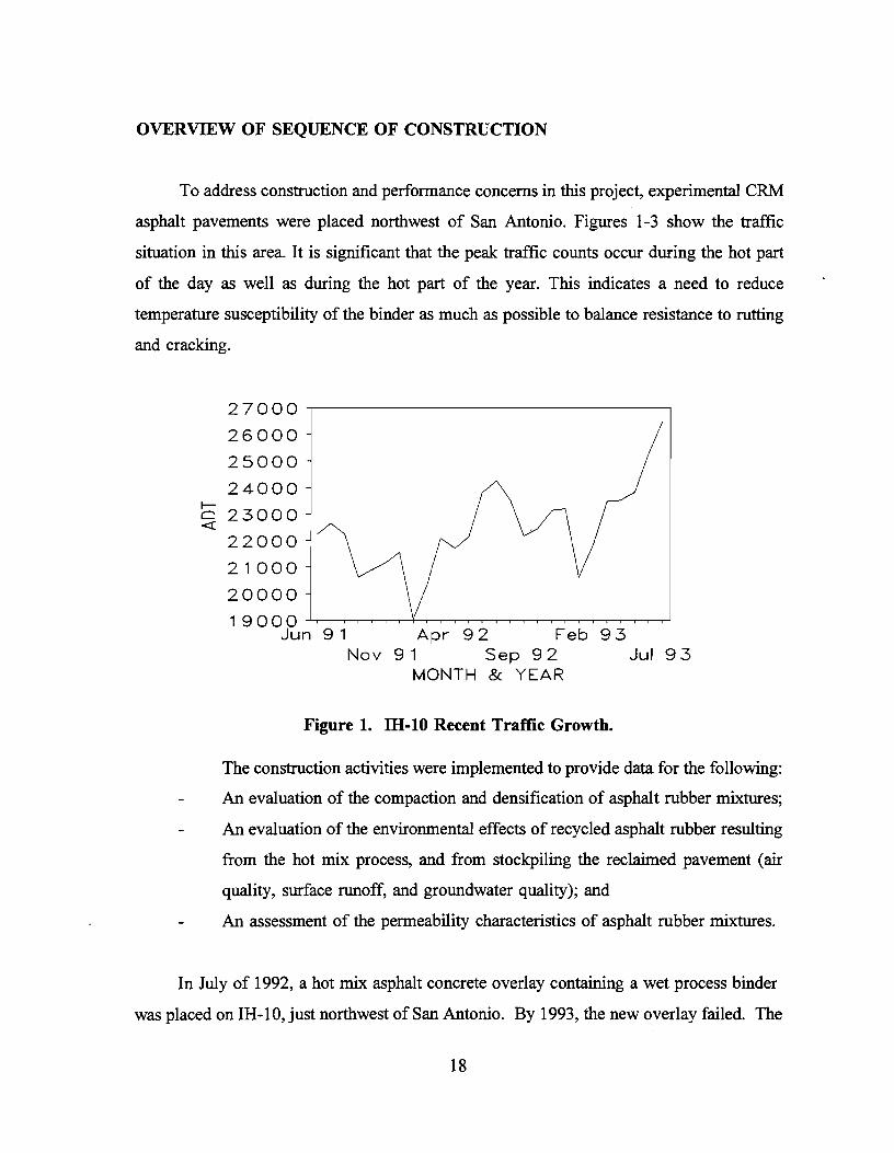
OVERVIEW OF SEQUENCE OF CONSTRUCTION
To address construction and performance concerns in this project, experimental CRM
asphalt pavements were placed northwest of San Antonio. Figures 1-3 show the traffic
situation in this area. It is significant that the peak traffic counts occur during the hot part
of the day as well as during the hot part of the year. This indicates a need to reduce
temperature susceptibility of the binder as much as possible to balance resistance to rutting
and cracking.
1--0 <(
27000
26000
25000
24000
23000
22000
21000
20000
19000 Jun 9 1 Apr 92 Feb 93
Nov 9 1 Sep 92 Jul 93 MONTH & YEAR
Figure 1. IB-10 Recent Traffic Growth.
The construction activities were implemented to provide data for the following:
An evaluation of the compaction and densification of asphalt rubber mixtures;
An evaluation of the environmental effects of recycled asphalt rubber resulting
from the hot mix process, and from stockpiling the reclaimed pavement (air
quality, surface runoff, and groundwater quality); and
An assessment of the permeability characteristics of asphalt rubber mixtures.
In July of 1992, a hot mix asphalt concrete overlay containing a wet process binder
was placed on IH-10, just northwest of San Antonio. By 1993, the new overlay failed. The
18

2000 l 1600
I- 1200 0 <:( 800
400
0 ..J....,-~-~~~--~~~-~~~~-r-'
1--Cl <:(
00 04 08 1 2 16 20
25000
24000
23000
22000
21000
20000
19000
02 06 10 14 1 8 22 HOUR OF DAY
)( Weekdays -- Weekends
Figure 2. IH-10 Daily Traffic Counts.
\
Dec Feb Apr Jun Jan Mar May Jul
Aug Oct Sep Nov
MONTH
Figure 3. IH-10 Monthly Traffic Counts.
19

signs of distress included alligator cracking, rutting, and pumping of fine material. Right
wheel path rut depths at four locations averaged between 0.8 and 14.7 mm (0.03-0.58 in.)
with the deepest rut measurement being 27.7 mm (l.09 in.). These same symptoms were
noticed at other locations, including on a section of IH-20 between Longview and Tyler.
Some have attributed these problem areas to the rubber in the mixtures. However, the
presence of rubber alone cannot be the sole perpetrator of the problems as the following
observations show: (1) many overlays that do not contain any rubber at all exhibit the same
symptoms of distress which may be related not only to the material characteristics but also
to characteristics of the bond between the overlay and the previously existing surface, and
(2) rubberized seal coats and some hot mix asphalt concrete (e.g., Loop 323 in Tyler, and
the frontage road on IH-10) appear to be performing well.
On IH-20 in Tyler, a small size, dense graded siliceous aggregate was used in the mix.
On the original IH-10 job, a small size aggregate was used at the start of the job, but by the
end of the job, a larger limestone aggregate was in use and the gradation had been changed
from dense to what may be described as a gap graded material, and the binder content was
increased to give the desired film thickness. This basic concept for ensuring stone on stone
contact throughout the aggregate fraction retained on the 2 mm (No. 10) sieve, and for
ensuring sufficient binder to give the desired film thickness to resist environmental damage
is the background for the material that the Texas Department of Transportation (TxDOT)
now refers to as CMHB (Coarse Matrix, High Binder) mixtures. It turns out that one of the
advantages of the rubber in the mix is that it helps to prevent drain-down of the asphalt
binder in these high binder mixtures.
By the end of the San Antonio overlay job, it had become apparent that the coarser
matrix material would be a better performer. Not only was the stone skeleton more
substantial in this mix, but the compaction process was better as well. The finer, dense
graded material used at the start of the IH-10 job was difficult to compact and resulted in
high and spatially variable air void contents, probably due to both rebound of the rubberized
mix and bridging across the uneven transverse profile of the previously existing surface by
the drum rollers. It is thought that the high air void contents connote higher permeabilities
which can lead to moisture assisted damage in the layer of interest as well as at the interface
20

between the overlay and the previously existing pavement. When the overlay later failed,
the starting point for the new mix design was the coarse, gap graded material used at the
end of the first job. TxDOT conducted extensive laboratory work on the designs and placed
a test section on Loop 1604 in the spring of 1993. Based on the favorable results from the
last portion of the first IH-10 job, the Loop 1604 test section, and additional laboratory
testing, the decision was made to recycle the mix in the failed sections on IH-10. The plan
was to mill the outer lane of the failed material and to take this reclaimed asphalt to a plant
where it would be added to new aggregate and asphalt in such a way that a material similar
to a CMHB would result for placement in the inlay. The plan was implemented in the fall
of 1993, and the material is performing satisfactorily at this time. The surface texture is
coarse, and water drains from the pavement for a considerable time after a rainfall event,
but no distress is apparent at this time. The final mix used on the recycle contained 30%
RAP, 5.7% asphalt, and 79.6% (by weight) aggregate retained on the No. 10 (2 mm) sieve.
21

II. PROCESS AND MATERIALS EVALUATION
ENVIRONMENTAL ISSUES
There has been some concern that the mandated use of waste tire rubber will create
an even worse environmental problem when the material must be recycled in the future than
now exists. Specifically, air quality might be adversely affected during the production
process, and water quality might be affected due to leaching in RAP stockpiles and under
the pavements. Aged or weathered asphalt pavement is different from new asphalt pavement,
and the addition of modifying agents to restore asphalt properties will change the chemical
composition of manufacturing and application emissions. In general, aging is accompanied
by reactions which essentially increase the asphaltene content. Asphaltenes are large,
complex nonpolar molecules (Bloomquist 1993).
While the number of detections possible in a volatile emissions sampling operation
can be phenomenal, the evaluation of their impact concentrated on a few materials are
known to be hazardous to the environment. Among these are polyaromatic hydrocarbons
(PAHs) which include naphthalene, fluorene, anthracene and benzopyrenes. Other
compounds are volatile organic compounds (VOCs), benzene, styrene, 1-2 butadiene,
phenanthrene, and particulates (Bloomquist 1993).
For the first generation of the IH-10 construction, the CRM asphalt concrete was
produced by the wet process in a drum mixer at the Redland Stone Products Company in
San Antonio. Southwestern Laboratories (SWL) sampled the hot mix operation and tested
for air emissions using standard EPA sampling techniques. The plant was equipped with a
baghouse rather than a scrubber and operated at a production rate of 351,080 kg/hr (387
tons/hr) during the sampling. For comparison, samples were also taken at the Duininck
Brothers hot mix plant. Testing was achieved in three separate sampling trains. Condition
1 was at a high temperature of 163°C (325°F) with a CRM mix; Condition 2 was at a low
temperature of 149°C (300°F) with a CRM mix; and Condition 3 was at a high temperature
23

with a conventional mix containing no CRM. Three trials were conducted for each test
condition. Trials for volatile organic sampling train (VOST) chemicals lasted 20 minutes,
and trials for other compounds lasted 60 minutes. Emission rates were calculated as pounds
per hour.
Emission rates at the Redland Stone plant are shown in Appendix B. The only
semivolatile organic chemicals detected in the conventional hot mix were 2-methyl
naphthalene, naphthalene, and phenanthrene. Emissions of VOST compounds decreased with
temperature and were higher during the mixing of CRM asphalt concrete than during the
conventional mix operation. A statistical analysis of variance of the air emissions data
showed that overall, there is very little difference in emissions from CRM plants versus
standard asphalt plants, as shown in Table 2.
Table 2. Statistical Analysis of Air Emissions Data at Two Texas CRM Plants.
Factor v Benzene Styrene Naph- 2- Phenan- Butadiene Particu- Opacity 0 thalene Methyl- threne !ates c Naphthalene
Plant N s N N s s s N N
Temperature N s N N N s N N N
%CRM N N N N N s N N N
N = not statistically different, S = statistically different
The only case in which 18% rubber resulted in higher emissions than no rubber was
for phenanthrene, but this may be attributed to the fact that 44% of the total possible
number of observations was missing for this compound. In some cases, measurements
showed a higher concentration of a compound at the low temperature condition than at the
high temperature condition, which is highly unlikely. A discrepancy of this sort may well
24

be the result of some variation in the hot mix plant operation itself or in the experimental
technique, rather than the chemistry of the materials. It should be noted that hot-mix asphalt
production is, by nature, a highly variable process, dependent on parameters such as the
fueling rate of the dryer, mix temperature, asphalt throughput rate, and asphalt binder
content, which are all themselves subject to variation (Bloomquist 1993).
In light of this high variability, it can at least be argued that for most chemicals, the
effect of CRM on emissions may be relatively small compared to the effects of other
variables. In two Ontario studies of environmental emissions, the levels of P AH emissions
were higher during the mixing of rubber-modified asphalt concrete than during the mixing
of conventional hot mix asphalt, while VOC emissions were lower. A Parmer County,
Texas, study showed that VOC emissions were slightly lower for the rubber mixture. The
limited sampling performed in this study was inadequate to assess emissions from mixing
of asphalt pavements with satisfactory precision, as is shown by the erratic nature of the
sampling results. Extensive sampling would be required to determine emission rates with the
degree of precision necessary to differentiate between emissions from conventional and
modified asphalt pavements.
Southwestern Laboratories (SWL) also performed leachate testing to determine the
potential for CRM to contaminate surface runoff and groundwater. From the recycled asphalt
rubber stockpiled at the Colorado Materials site in New Braunfels, Texas, a sample was
transported to the laboratory and was subjected to a simulated precipitation leachate which
is expected to represent the lifetime cumulative effect of acid rainwater leaching. The
simulated precipitation leachates were analyzed for trace metals, volatile organic compounds,
and semivolatile organic compounds.
Results from the leachate analysis showed that the only constituent occurring at levels
above the detection limit was mercury, which was detected at 0.0011 mg/I. This level is
below the current EPA drinking water limit for mercury (0.002 mg/I). A table of all the
trace metals tested for is provided in Appendix B, which shows that all other compounds
tested for were below the analytical detection limit. From these findings, it can be concluded
that trace metals, volatile organics, and semivolatile organics may be leached from asphalt
rubber, but at levels too low to be environmentally significant or hazardous.
25

SWL performed emissions sampling for the recycled CRM mix at the Colorado
Materials Company site in New Braunfels, Texas, during the months of October and
November 1993. Conditions were similar to the Redland Stone operation: Condition 1 - low
temperature - <149°C (300°F) with recycled CRM; Condition 2 - high temperature > 149°C
(300°F) with recycled CRM; Condition 3 - high temperature >149°C (300°F) with
conventional hot mix asphalt. The CRM mix consisted of 30% RAP, and both mixes had
an average asphalt content of 5.3%. Because temperature requirements at the field site
limited the low temperature range of the mix, no testing was performed on Condition 1.
PERFORMANCE RELATED CHARACTERISTICS
Original IB-10
Most of the studies concerning long-term performance of the mix were done in the
laboratory. The original IH-10 overlay built in July 1992 had a mixture design consisting
of 7.5% AC-10 and 18% crumb rubber by weight of the binder in the wet process. During
construction, samples of hot mix CRM asphalt were obtained and sieve analyses were run
in the field lab. Cores molded from the samples were also tested for density and specific
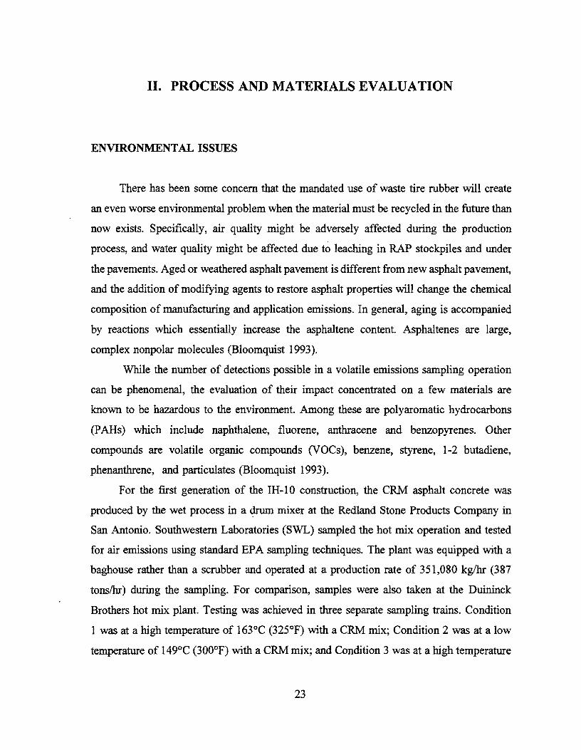
gravity. The mixture varied from a dense gradation (59% retained on the No. 10 sieve) to
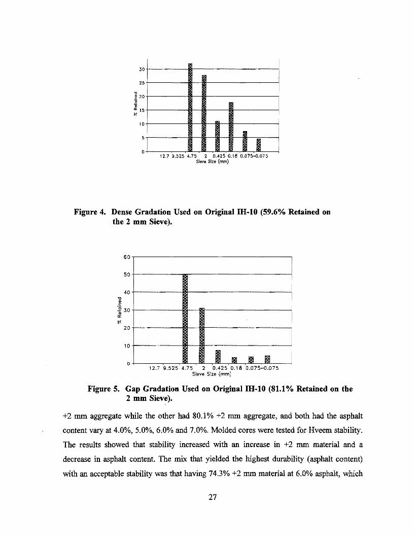
a gap gradation (81.1% retained on the No. 10 sieve) at the end of the job, with asphalt
contents ranging from 7.0 to 8.5%. Figures 4 and 5 show a comparison of these gradations.
Samples were taken from the truck at Redland Stone to the District Materials and
Tests Division Lab, molded into cores, and tested for Hveem stability, Rice specific gravity,
and gradations. In San Antonio, residency personnel obtained thirty cores from different
positions relative to the wheel path and took nuclear density measurements.
Recycle Test Pavement
David Kight performed experimental mix designs at the Redland Division Laboratory
in March of 1993. Two gap graded mixes using 30% RAP were compared. One had 74.3%
26
30
25
10
5
0 I 12.7 9.525 4.75 2 0.425 0.18 0.075-0.075
Sieve Size (mm)
I I
I
Figure 4. Dense Gradation Used on Original IH-10 (59.6°/o Retained on the 2 mm Sieve).
60
50
40 "O ., c: ] 30 ., 0::
~
20
10
0 I rm I I
12.7 9.525 4.75 2 0.425 0.18 0.075-0.075 Sieve Size (mm)
I
Figure 5. Gap Gradation Used on Original IH-10 (81.1% Retained on the 2 mm Sieve).
+2 mm aggregate while the other had 80.1% +2 mm aggregate, and both had the asphalt
content vary at 4.0%, 5.0%, 6.0% and 7.0%. Molded cores were tested for Hveem stability.
The results showed that stability increased with an increase in +2 mm material and a
decrease in asphalt content. The mix that yielded the highest durability (asphalt content)
with an acceptable stability was that having 74.3% +2 mm material at 6.0% asphalt, which
27

gave a stability of 38. Specification values usually range from 30-37 minimum. A test
section was constructed on Loop 1604 with a final mix design that contained 30% RAP,
5.8% asphalt cement, and 74.3% limestone aggregate retained on the 2 mm sieve.
CRM Recycle
Prior to the recycling phase, several type "C" CMHB mix designs were experimented
with, using 30% RAP, AC-20, and a gap gradation. For a particular mixture containing 79%
+2 mm material, five asphalt contents were varied from 4.5% to 6.0%. Hveem stability,
Rice specific gravity, and VMA were measured. Finally, in October 1993, the outer lane of
the failed overlay was milled and sent to Colorado Materials Co. in New Braunfels, where
it was used in a mix containing 30% CRM RAP, 5.7% AC-10, and 79.6% aggregate
retained on the 2 mm sieve. Sieve analyses were run on material entering the cold feed bins.
Samples from the hot mix operation were molded into cores that were analyzed for
gradation and tested for Hveem stability, specific gravity, nuclear asphalt content, and creep.
The percent +2 mm aggregate and the Hveem stability were plotted against air voids, creep
strain, and creep stiffness, but no definite relationships were found.
Compaction Studies
To quantify changes in physical characteristics of CRM mixtures during the
densification process, a factorial design was implemented. Three mix designs and several
construction conditions were included in the design, giving a total of 51 tests. The tests
performed were in general accordance with the ASTM D3387: Standard Test Method for
Compaction and Shear Properties of Bituminous Mixtures by Means of the U.S. Corps of
Engineers Gvratorv Testing Machine (GTM). The U.S. Army Engineer Waterways
Experiment Station (WES) undertook this task.
WES provided data on GTM revolutions, unit weight, and a gyratory stability index
(GSI) for each test at a frequency of 10 revolutions for a total test period of 250 revolutions.
28

Some background on this test procedure is presented here so as to enhance understanding
of the significance of the results obtained by WES and the conclusions drawn.
The development of the GTM originated at WES and has continued at the Engineering
Developments Company (EDCO) (McRae 1993). The GTM is a combination compaction
and plane strain, simple shear testing machine for use on soils, base course materials, and
bituminous type-paving materials. The gyratory shear it provides is a more uniform shear
strain than the direct shear and triaxial shear achieved with conventional testing equipment.
Two of its several applications include:
1) Providing a testing machine in which theoretical vertical stress at any depth
within the structure can be introduced for compaction and shear testing; and
2) The production of test specimens by a kneading compaction process which
gives stress-strain properties representative of actual compacted bituminous
pavement.
TxDOT uses a version of the Hveem stability to evaluate the adequacy of asphalt
mixtures. A stability of 35 is often recommended as a minimum for adequate performance.
Specification values usually range from 30-37 minimum, depending on the expected traffic
for which the pavement is being designed. Because CRM mixtures sometimes have low
stabilities when measured with the standard test, and because the stability test does not
provide much information with respect to compaction, additional tests were conducted to
further explore the material behavior.
Samples of the original IH-10 CRM overlay, the Loop 1604 CMHB and 30% RAP
mixes, and the final IH-10 inlay materials were tested in the GTM. For the experiment
design, thirteen combinations of three loading pressures and three temperatures were used.
The low (L ), medium (M), and high (H) pressures were 517 k:Pa (75 psi), 1034 k:Pa (150
psi), and 2068 k:Pa (300 psi), to simulate a range of traffic wheel loads. To simulate truck
(T) and roller (R) compaction, loading pressures of 1207 k:Pa (175 psi) and 1551 k:Pa (225
psi) were used. The L, M, and H temperatures were 60°C (140°F), 121°C (250°F), and
l 60°C (320°F) to cover the range of temperatures expected from hot summer pavement
29

temperatures to temperatures during laydown. Table 3 shows the experiment design. Table
4 shows the ending gyratory strain, the GSI, and the GCI for each sample. Figures 6 and
7 illustrate that the mixtures are easy to compact and that there is a relationship, albeit
accompanied by high variability, between Hveem stability and the gyratory shear strain (a
form of engineering shear strain) at the end of the compaction. The GSI measured in the
GTM was greater than 1.0 in all except one test. That test was a 517 kPa (75 psi) test, and
our computations indicate that a 36,287 kg (80 kip) truck would be closer to a 1207 kPa
(175 psi) vertical pressure in the GTM. Values of GSI greater than 1.0 generally indicate
excess asphalt content or some other physical characteristic that results in undesirable
plasticity.
Table 3. Factorial Design for Compaction Study.
RAP PRESSURE TE1\.1PERA TURE (°F) CONTENT (%)
(kPa) (psi) 6o·c 121 ·c 16o·c (320°F) (140°F) (250°F)
517.l 75 SLM 0
1034 150 SML SMM SMH
2068 300 SHM
517.1 75 SLM
30 1034 150 SML SMM SMH
2068 300 SHM
517.l 75 SLM
100 1034 150 SMM
2068 300 SHM
1207 175 STL STM 30
1551 225 SRL SRM
IL= low M =medium H= high T =truck R =roller I
30

Table 4. Results of Gyratory Testing.
Specimen ID CRMRAP Gyratory GCI GSI Gg (psi) Content Angle
(%) (degrees)
SHMO.Rl 0 2.81 0.9930 2.23 4247 SHMO.R2 0 2.54 0.9894 2.14 4027 SHMO.R3 0 2.36 0.9894 1.95 3385
SMHO.Rl 0 1.82 0.9678 1.51 2403 SMHO.R2 0 1.72 0.9763 1.39 3154 SMHO.R3 0 1.94 0.9763 1.60 3462
SMMO.Rl 0 2.13 0.9797 1.68 2915 SMMO.R2 0 2.10 0.9813 1.66 3301 SMMO.R3 0 1.94 0.9784 1.54 3481
SMLO.Rl 0 1.94 0.9751 1.54 3993 SMLO.R2 0 2.01 0.9717 1.51 3933 SMLO.R3 0 1.95 0.9721 1.48 3550
SLMO.Rl 0 1.34 0.9650 1.01 3759 SLMO.R2 0 1.34 0.9676 1.01 3693 SLMO.R3 0 1.30 0.9650 0.96 4270
SHM3.Rl 30 2.61 0.9914 1.79 4126 SHM3.R2 30 2.17 0.9906 1.60 4369 SHM3.R3 30 3.03 0.9916 1.70 6315
SMH3.Rl 30 2.26 0.9850 1.54 2376 SMH3.R2 30 2.17 0.9809 1.51 2557 SMH3.R3 30 2.34 0.9863 1.72 1918
SMM3.Rl 30 2.26 0.9875 1.61 2563 SMM3.R2 30 2.37 0.9825 1.62 2285 SMM3.R3 30 2.06 0.9771 1.46 3277
SML3.Rl 30 2.18 0.9751 1.49 2800 SML3.R2 30 2.44 0.9761 1.64 2672 SML3.R3 30 2.35 0.9775 1.58 2637
31
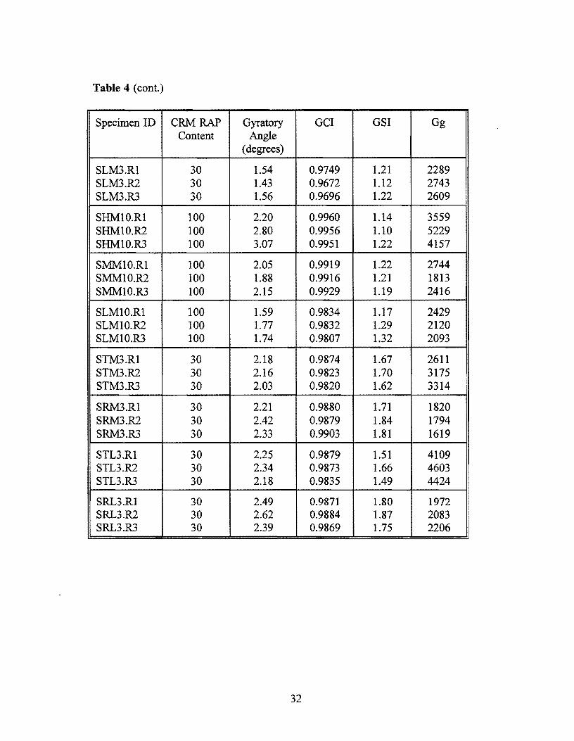
Table 4 (cont.)
Specimen ID CRM RAP Gyratory GCI GSI Gg Content Angle
(degrees)
SLM3.Rl 30 1.54 0.9749 1.21 2289 SLM3.R2 30 1.43 0.9672 1.12 2743 SLM3.R3 30 1.56 0.9696 1.22 2609
SHMlO.Rl 100 2.20 0.9960 1.14 3559 SHM10.R2 100 2.80 0.9956 1.10 5229 SHM10.R3 100 3.07 0.9951 1.22 4157
SMMlO.Rl 100 2.05 0.9919 1.22 2744 SMM10.R2 100 1.88 0.9916 1.21 1813 SMM10.R3 100 2.15 0.9929 1.19 2416
SLMlO.Rl 100 1.59 0.9834 1.17 2429 SLM10.R2 100 1.77 0.9832 1.29 2120 SLM10.R3 100 1.74 0.9807 1.32 2093
STM3.Rl 30 2.18 0.9874 1.67 2611 STM3.R2 30 2.16 0.9823 1.70 3175 STM3.R3 30 2.03 0.9820 1.62 3314
SRM3.Rl 30 2.21 0.9880 1.71 1820 SRM3.R2 30 2.42 0.9879 1.84 1794 SRM3.R3 30 2.33 0.9903 1.81 1619
STL3.Rl 30 2.25 0.9879 1.51 4109 STL3.R2 30 2.34 0.9873 1.66 4603 STL3.R3 30 2.18 0.9835 1.49 4424
SRL3.Rl 30 2.49 0.9871 1.80 1972 SRL3.R2 30 2.62 0.9884 1.87 2083 SRL3.R3 30 2.39 0.9869 1.75 2206
32

a.994
CL 99 t o. 986
~ o. 962 t " "'
0.97S
t .:1.974
o. 97
30 100
RAP Content. {$)
Figure 6. Compactibility Index For Materials Tested in the Experiment.
G ~
"' o. a ~ < .d ... ~
"' 0. 6
~ " -;; !: 0 .• .. " ..
o. 2
10 zc 30 40 50
llvee• Stability
Figure 7. Ending Gyrograph Reading and Hveem Stability (All Mixes in the Experiment Combined).
33

These findings raise some question as to the prospects for rutting and flushing of the mix
and the associated safety and performance degradation. Further testing was performed at TTI
to determine specific gravity, air voids, and Hveem stability. The summary in Appendix B
provides data on these tests. The results show that generally, the air voids decrease as the
pressure increases from 517 kPa (75 psi) to 2068 kPa (300 psi) at a given temperature in
the gyratory test. As Figure 8 illustrates, the finer graded 100% RAP shows a more rapid
reduction in air voids than the larger, coarser CMHB (0% RAP). For the 100% RAP
material at 250 gyrations, 2068 kPa (300 psi) and 121°C (250°F), the air void content is
essentially zero (0.17%), while at 517 kPa (75 psi) and 1034 kPa (150 psi), the air voids
were 2.8% and 1.4% for the same mix.
18
16
14 GTM Data @2068 kPa @ 121 C
12 ,-.. ~ ......, U1 10 0 0 > 8 a:: <{
6
4
2
50 100 150 200 250 GYRATIONS
I~ 0% RAP -+- 30% RAP """"*""" 100% RAP
Figure 8. Air Voids vs. Gyratory Revolutions.
34

This trend indicates that the recycled CRM asphalt would be suitable for car and light
truck traffic, but may show rutting or bleeding under heavy truck traffic. These results may
be compared with the results shown by Roberts et al. (1991) and illustrated in Figure 9. The
satisfactory performance of recycled CRM mixtures thus seems to depend on ensuring stone
on-stone contact. This might best be achieved by gap- and open-graded mixtures such as
CMHB or SMA (Stone Matrix Asphalt) materials. The potential for segregation in this type
of mixture seems to be alleviated by thick films of asphalt and by the presence of CRM,
which helps prevent draindown of the binder.
8
en 7 Cl i5 > I- 6 z w u a:: w CL 5
4
• ~!5 BLOWS. PLANT lMECHJ
•
• ---· 3a~----~I0~----~2~0--------:;3~0:-----::4~Q------:5~0:----:6~0-------,.,l70 NUMBER OF GYRATIONS
Figure 9. Air Voids vs. Gyrations at 689 kPa (100 psi) Compaction Level (after Roberts et al. 1991).
Permeability Characteristics
Water permeability of paving mixtures has always been important. Construction of
zero permeability paving materials is elusive if not impossible. However, surfaces can be
made with very low permeabilities and geometries that effectively make the pavement
impermeable. At the other extreme, materials can be placed that have permeabilities high
enough to act as drainage facilities and which do not support high pore pressures because
there are relatively continuous paths through the pore structure to an exit. Between these
35

two extremes lies the material that allows water into its internal structure and then proceeds
to self-destruct under the cycling of pore pressure caused by traffic (augmented in some
locations by damage associated with freeze-thaw cycles). The CMHB material actually has
some of the characteristics of both of the extremes. The gradations used for the CMHB
begin life with porous characteristics. Then the pore structure is filled with the fine
aggregate fraction and rubberized binder.
Since there is no outlet for water on the San Antonio IH-10 test section because of
the inlay technique, near zero permeability is necessary to prevent waterlogging in layers
below the wearing course. An important factor affecting the permeability of asphalt
pavements is the air void ratio, so it was of interest to define a relationship between air void
ratio and permeability. Since there is no standard test procedure to test the permeability of
bituminous mixtures, a procedure was developed as a modification of ASTM D 2434:
Permeability of Granular Soils (Constant Head). The modified procedure prescribes a
constant head method for dense mixes with less than 3% air voids, and a falling head
method for open mixtures with higher air void contents.
The test method determines the coefficient of permeability for the laminar flow of
water through the asphalt rubber. To ensure laminar flow under constant-head conditions,
the ideal test conditions necessary are:
1) Continuity of flow with no volume change during a test,
2) Flow with the air voids saturated with water, and
3) Flow in the steady state with no changes in hydraulic gradient.
The permeameter used in this study was built in the TTI machine shop, with a minimum
internal diameter of 5.0 cm (2.0 in.) and a maximum of 10.0 cm (4.0 in.), which is the size
of standard molded specimens of asphalt concrete. Details of the test procedure are provided
in Appendix A. From the determination of air void ratios on the mixes tested by WES,
specimens with the highest and lowest air void ratios were selected for permeability tests.
Nine samples were tested for permeability in multiple runs. Five of the specimens
were GTM samples, and the sixth was a field core cut from the original CRM mix laid on
36

IH-10. The range of air void ratios for all six specimens (0.292 to 3.049) was too small to
realize any trends occurring, so it was necessary to mold new specimens having higher air
void ratios. Five additional points were thus obtained from cores molded at 4.5%, 5.0%,
6.0%, 8.3%, and 10.0%. A multiple regression analysis was performed on the data, giving
an R2 value of 0.98 and the following linear relationship:
logk - -2.31 + 0.41 logvoids+ 1.95 loggradient. (1)
Figure 10 shows a graph of how permeability would vary with percentage air voids at a
fixed gradient of 0.1. The results exhibit an expected overall relationship of permeability
increasing with air void ratio, the k values for all eleven data points falling below 104
emfs.
0.00016
0.00014 • ,,..-.._ 0.00012 •
(/) • ""' 0.0001 • E (.) .r .._,__,,
SE-05 ~ •
6E-05 • • 4 E -0 5 1a9 k = -2.31 + 0.41 log voids + 1.95 log gradient
2E-QS-1--..--~~~~~~~___.
0 2 4 6 8 10 % Air Voids
Figure 10. Permeability of CRM Asphalt vs. Air Voids (Gradient= 0.1, Falling Head Method).
37

While permeability and air void content are often assumed to be directly proportional,
it must be stressed that a mixture with high air voids could easily have a low permeability,
due to certain size dimensions of the individual voids and the lack of interconnection of the
voids (Zube 1962). In Figure 10, the value of k appears to level off as air void content
increases, suggesting that for the very open mixtures where the voids were connected at a
maximum, the coefficient of permeability was limited by the maximum flow rate attainable
by the apparatus. For the denser mixtures, the smaller the number of air voids present, the
more the permeability depends on those few voids being well-connected. This explains why
for two samples with comparable air void contents, the coefficient of permeability may be
vastly different, as seen in Table 5. Apparently, the 30% RAP specimens have thicker
asphalt films and thus fewer interconnected voids than those with 100% RAP at comparable
air void contents. This reduction in permeability from first to second generation is favorable
to the specific drainage needs of the recycle test section, which would be prone to moisture
assisted damage if the inlaid pavement were highly permeable.
Permeability and average velocity were plotted against average gradient. The
relationship obtained appears to be linear where the gradient ranges from 0 to 0.4, as shown
in Figure 11. This confirms laminar flow for low gradients and validates the use of Darcy's
Law in this region.
Table 5. Dependence of k on Air Voids Interconnectivity.
I % RAP in Sample I Air Voids(%) I k (emfs) I 100 (original 1-10) 1.345 7.124x 10⁻⁴
30 (recycled) 0.996 1.048 x 10⁻⁴
100 (original) 3.3 1.403 x 10'3
30 (recycled) 3.049 5.537 x 10·5
38

Permeability vs. Gradient, Velocity - For CRM RAP, varying % rubber r.n Q
"'- 1.OE-01 1 .OE+OO -E x iii ::: r.n ~x
- "'-1 .OE-02 - -u -- E 1 .0 E-0 1 E '--"" x
1 .OE-03 'Ii !:= u ~ ~ 1 .0 E-0 2
'--""
1 .OE-04 • >-•X -x 1 .OE-03 u
1 .OE-05 0 ().)
!.... 1 .OE-06 1 .OE-04 > ().)
0 0.4 0.8 1 .2 1 .6 CL
Gradient
- Permeability x Velocity
Figure 11. Permeability vs. Gradient and Velocity (Falling Head Method).
Creep and Compression Characteristics
CRM asphalt concrete is viscoelastic, possessing both an elastic component and a
time-dependent viscous component that causes this material to flow gradually when subject
to traffic. Creep testing measures time-dependent permanent deformation of CRM asphalt
concrete. The unconfined compression strength is a measure of the maximum vertical load
sustainable by a specimen before failure. The GTM compacted specimens which were tested
for permeability were also tested for creep and compression strength in accordance with test
methods TEX-231-F and AASHTO T-167. Table 6 provides a summary of the results from
the creep test. More extensive data from creep testing of field cores and additional lab
molded specimens can be found in the Appendix B. The variation of creep stiffness with
CRM RAP content is shown in Figure 12.
Data from compression testing is given in Table 7, and Figure 13 shows the variation
of compression strength with RAP content.
39

Table 6. Uniaxial Creep Test Results.
Specimen CRMRAP Total Strain Pennanent Slope of Creep Creep ID Content Strain SS portion Compliance Stiffness
(%) (1/sec) (1/kPa) Modulus smlx (kPa)
SLMO.R3 0 6.649x10⁻⁴ 2.047x10⁻⁴ 2.100x10"8 9.724x10.., 102835
PAVE 0 l.367x10·3 4.288x10⁻⁴ 5.200xl0·8 2.007x10⁻⁴ 49835
SML3.Rl 30 2.317x10·3 1.417xl0·3 1.640xl0·7 3.378xl0-4 29599
STL3.R3 30 1.845x10·3 l.197x10·3 1.490x10"7 2.697x10⁻⁴ 37080
SRM3.R3 30 l.747xl0·3 l.022xl0·3 l.080xl0·7 2.549xl0-4 39231
SHM10.R3 100 3.315x10·3 2.054x10·3 2.260xt0·7 4.830x10⁻⁴ 20705
120000
100000
'O' a.. .:::=..
80000 (/) ::I
"5 -0 0
::E
"' (/) 60000
"' :E v; 40000 0.
"' "' ... u
20000
0 0 0 30 30 30 100
CRM RAP CONTENT (%)
Figure 12. Variation of Creep Stiffness with Percentage CRM RAP.
40

Table 7.
3.R3
STL3.R3
SRM3.R3
SPEC.3
SHMIO.R3
Compressive Strength Test Results.
5000
c Q.
04000 .s: a. " ..
<7i 3000 .. > ;; .. .. ~2000 0
<..>
1000
0
CRM RAP Content (%)
0
0
30
30
30
100
Q 30 30· 30 CRM RAP Conlent (%)
pression Strength
4806.2
4302.5
4983.0
5840.0
4983.0
4559.7
4488.5
100 30
Figure 13. Variation of Compressive Strength with CRM RAP Content.
41

BINDER CHARACTERISTICS
. Asphalt-rubber samples (asphalt meaning either asphalt or recycling agent) were aged
under numerous conditions. The samples were POV-aged under 345 kPa (50 psia) of
nitrogen and 93°C (200°F), under atmospheric air and 93°C (200°F), or under 2068 kPa
(300 psia) of oxygen and 82°C (180°F) or 93°C (200°F). The samples were oven-aged with
atmospheric air at either 49°C (120°F) or 163°C (325°F). To fully understand the
difficulties of aging asphalt-rubber, a detailed explanation of research to date is required.
Nitrogen-Aged Samples
Asphalt-rubber samples were nitrogen-aged to determine if the samples cure, defined
as an increase in viscosity without a corresponding increase in carbonyl area, when exposed
to high temperatures. If the samples were found to cure at the high temperatures found in
the POV, it would drastically complicate using the POV for an aging test. Diamond
Shamrock AC-5, SHRP ABM-1, and blends of 10% and 18% or 20% of each asphalt were
aged under 345 kPa (50 psia) of nitrogen and 93°C (200°F). The viscosity and the carbonyl
area of the asphalts and the asphalt-rubber blends were determined to remain constant with
aging time. This can be seen in Figure 14 and Figure I5, respectively. GPC analysis of
the samples that were incubated under nitrogen also shows that no type of curing or aging
occurs. This is shown in Figure I6 for the SHRP ABM-I asphalt and in Figure I 7 for the
18% by weight Rouse -0.425 mm mesh and SHRP ABM-I asphalt-rubber. The asphalt acts
like a solvent for the rubber, and because the rubber is crosslinked, it cannot dissolve or
degrade, but can only swell. Apparently the swelling is caused by the rubber-asphalt bonds
forming and/or replacing the strong secondary bonds of the rubber. However, the
crosslinked polymers are not soluble because the solvent cannot overcome primary valence
crosslinks, and thus the dissolution or degradation of the rubber does not occur. This
contrasts with what occurs during mixing, with the material of the 20 to 25 retention time
region increasing with mixing. This is shown in Figure I8 for a Fina AC-5 asphalt and Tire
Gator -0.425 mm mesh mixing (curing) study. From the curing studies, it is known that a
binder's viscosity increases and the carbonyl area remains constant when mixing under a
42

t> IP "' 15000 ::0
----b·------------~----~ ~~
l!! -e-DSAC·S -i3 · 10190, TG.-40, OS AC-5 - ~ • 20180, TG -40, OS AC-5
ol5 10000
Aged with 34S kPa (SO psia) of Nitrogen at 93'C (200'F)
• ·X • • SHRP ABM·1 -
u c c IQ
• i:-
· · + · · 10/90, RS -40, SHRP ABM· 1 --t.- • 18182. RS -40, SHRP ABllA·1
....... ·+· ...... ·+· ....... -t •....... + ....... . 5000 0
----~----~--------~------------x--------x-~~-----X--------x--------
1.-- - -a- - ~ - ~- - cr- - ~~ 0 ~~~~ ......... ~~~---'-~~~~.._~~~--"-~~~---'
0 , 2 3 4 5
TIME (DAYS)
Figure 14. Viscosity Data of Nitrogen-Aged Samples.
< w a: <
, -. ..J > z 0 Ill
~ 0.5 0
0 D
Aged with 34S kPa (SO psia) of Nitrogen at 93 'C (200'F)
-e-DSAC-5 ·. -i3 · 10/90, TG -40, OS AC-5 -:- ._ • 20/80, lG -40, OS AC-5 - • x • "SHRP ABllA-1 · · + · · 1o,go, RS -40, OS AC-5 --t.- • 18182, RS -40, OS AC-5
-~----~----- ~ ::IC- =-=- =-;: =.: -·c- - ~ - - ! v Q II
' I I
2 3 4 5
TIME (DAYS)
Figure 15. Carbonyl Area Data of Nitrogen-Aged Samples.
43

0.8
w i:n 0.6 -
·Z 0 ll. i:n w-c: E
Ill
0.4 -c: ... o.!:" ... > 0.2 oE w-... w 0
0 c:
--NEAT - - • 1 DAY · · · · ·3 DAY ········· SDAY
20
Aged with 345 kPa (50 psia] of Nitrogen at 93•c (200"F)
25 30 35 40
TIME (MINUTES)
45
Figure 16. GPC Data of Nitrogen-Aged SHRP ABM-1.
0.6
0.5 w U)
z 0.4 0 ll. (I) 0.3 w-a: E
Ill c: .. 0.2 o.!:" ... > oE 0.1 w-... w 0 0
ir -0.1
-0.2 15
--NEAT - - • 1 DAY • • · ~ · 2 DAY · • · · ·3 DAY - · -· ·4 DAY
20
Aged with 345 kPa (SO psia) of Nitrogen at 93•c (200°F)
25 30 35 40 TIME (MINUTES) .
45
Figure 17. GPC Data of Nitrogen-Aged SHRP ABM-1 and Rouse-0.425 mm Mesh Blend.
44

w Cl) z 0 ll. Cl)
0.8 ...------1---........... --....---....----. --FINA AC-5, NEAT - ·CURED3HR • - - • • CURED 6 HR · ·.
0.6 ·---·CURED12HR · · • • • CURED22HR - - • CURED30HR - · - · • CURED 41 HR
Cured under Nitrogen Blanlcct at 163°C (3SO"F)
~E o.4 Ill
a: .. oE' ..,.> oE w-... w Q
a:
-0.2 __ __. ____________ ....._......__.....__ _ ___,
15 20 25 30 35 40 45
TIME (MINUTES)
Figure 18. GPC Data of Curing Study (Fina AC-5, Tire Gator -0.425 mm Mesh).
nitrogen blanket at 177°C (350°F). It is theorized that the high mixing temperature
enhances the rubber's degrading or reacting with the asphalt. At such a high mixing
temperature, the entropy factor of the Gibbs free energy change equation, LiG= LiH-Li TS,
dominates and thus makes the change in the Gibbs free energy negative, increasing the
spontaneity of the reaction. Additionally, the mixing apparently supplies the continual
dispersement that helps the rubber and the asphalt to chemically bond.
Oven or POV-Aged Samples
GPC Analysis
Asphalt-rubber samples were aged under various combinations of pressure and
temperature. Decomposition of the rubber into the asphalt part of the asphalt-rubber binder
occurs at all combinations of pressure and temperature. This is shown in Figures 19-21 for
SHRP ABM-1 asphalt-rubber blends, with Figure 19 representing high temperature and high
oxygen pressure conditions, Figure 20 representing high temperature and atmospheric
45

0.6 ""I
0.5 --NEAT POV Aged with 2,068 kPa (300 psia) w Ui - - • 1 DAY of Oxygen at 93°C (200°F) :z 0.4 ·····2DAY 0 • • • • • 3 DAY ll.
- ·- ··5DAY Ui 0.3" w-- ·········6DAY cc E • cct; 0.2 o-..,> oE 0.1 w-... w 0 Q
i:C ·0.1
·0.2 15 20 25 30 35 40 45
TIME (MINUTES)
Figure 19. GPC Data of SHRP ABM-1 and Tire Gator -0.425 mm Mesh Blend POVAged at 93°C with 2,068 kPa of Oxygen.
--SHRP ABU.1. NEAT - • 10i90. TG -40, SHRP ABM·1. NEAT • - • • • S DAY ·····12DAY · • • • • 160AY - - ·21 DAY
w Ui 0,4 :z 0 ll. 0.3 Cl) w--a: E
0.2 = cco o-..,> 0.1 uE w-... 0 w Q
£C -o. 1
-0.2 15
I
, :::-:f'' / ,' /, . , /
Oven Aged with 101 kPa (IU psia) of Air at 163°C (325"1')
1::.·~/_f
20 25 30 35 40
TIME (MINUTES)
45
Figure 20. GPC Data of SHRP ABM-1 and Tire Gator -0.425 mm Mesh Blend OvenAged at 163°C with 101 kPa of Air.
46

0.6 r---.---,---,.--~r-----.----.
w (f)
0.5
5 0.4 t1.
fil- 0.3 a: E
Ill
a: a. 0.2 -~> g! 0.1 ,...
--NEAT - - • 18 DAYS • • • - • 30 DAYS
. ••·••·•·· 40 DAYS
~ 0 ..,__ ___ _
·O. 1
Oven Aged with 101 k:Pa (14.7 psia) of Air at 49°C (l 20°F)
·0.2 :----:'::---:"-~----.,.....l..----'L....i;::..._---l. __ _j 15 20 25 30 35 40 45
TIME (MINUTES)
Figure 21. GPC Data of SHRP ABM-1 and Rouse -0.425 mm Mesh Blend Oven-Aged at 49°C with 101 kPa of Air.
oxygen pressure conditions, and Figure 2 I representing road conditions of summer road
temperature and atmospheric oxygen pressure. It is theorized that the decomposition of the
rubber into the asphalt is caused by oxidation involving chain scission of the completely
substituted carbon. This contrasts with what occurs in the mixer, where the rubber degrades
by thermal energy, and with what occurs in the POV under nitrogen, where the rubber does
not degrade, apparently because of the lack of oxygen.
Furthermore, the GPC analysis showed that the interaction of the rubber and the
asphalt depends largely upon the composition of the asphalt. Figures 19, 20, and 21 are
data of the decomposition of the rubber into the asphalt, SHRP ABM-I, that has significant
percentages of each of the four asphalt groups: asphaltenes, saturates, napthene aromatics,
and polar aromatics. Figures 22 and 23 are data of the POV-aging of SHRP ABM-1
Fraction and rubber/SHRP ABM-I Fraction, respectively. The SHRP ABM-1 Fraction is
a supercritical fraction of the SHRP ABM-I asphalt with the fraction being nearly saturate
and asphaltene-free. Figure 22 shows that the SHRP ABM-1 Fraction produces only small
47

LIJ Cl)
z 0 Q. U> LIJ -a: E
Ill a: .. o~ .,_> oE w-... w Q
a:
0.8
0.6
0.4 -
0.2
0
--1DAY - - -2DAY • • · • • 3 DAY ·······SDAY -·-··6DAY
Oven Aged with 2,068 kPa (300 psia) of Oxygen at 93°C (200"F)
·0.2 ,__ __ ..__ __ ....._ __ ..J.---....L---.....:.....--....1 is 20 25 30 35 40 45
TIME {MINUTES)
Figure 22. SHRP ABM-1 Fraction POV-Aged at 93°C with 2,068 kPa of Oxygen.
0.8
w CD 0.6 z 0 ll. (I) w-a: E
Ill
0.<4
a: .. o~ t-> ci:2 oE w-... w Q
0 c:
-0.2 15
--1DAY - - ·2DAY • • - • • 3 DAY ·••·•·· S DAY -· -··6DAY
20
Oven Aged with 2,068 kPa (300 psia) ·of Oxygen at 93•c (200°F)
25 30 35 40 TIME (MINUTES}
<45
Figure 23. GPC Data of SHRP ABM-1 Fraction and Tire Gator -0.425 mm Mesh Blend POV-Aged at 93°C with 2,068 kPa of Oxygen.
48

quantities of asphaltenes with aging. Figure 23 shows that the rubber decomposed into the
binder during curing and was further decomposed during aging, with the mass from the neat
binder curing peak being systematically moved into the longer retention time region with
aging time. Note the lack of influx of mass from the rubber with aging time as with the
whole asphalt/rubber binder. It is theorized that the lack of rubber decomposition during the
aging stage is caused by the absence of asphaltenes in the ABM-1 Fraction. Additionally,
Tire Gator -0.425 mm mesh rubber was cured with SUN Hydrolene 125, a recycling agent
containing manufacturer reported values of0.1%asphaltenes,13.5% polar aromatics, 70.9%
napthene aromatics, and 15.5% saturates. Figure 24 shows that the rubber in the SUN
125/rubber blend did not decompose upon aging, supporting the earlier theory that
asphaltenes must be present if the rubber is to be compatible with or soluble in the asphalt.
Hardening Susceptibilities
Previous work has shown that asphalt hardening susceptibilities, the slope of a log
viscosity versus corrected carbonyl area plot, are independent of POV temperature.
However, this work shows that asphalt-rubber hardening susceptibilities are dependent on
POV temperature. Figure 25 shows this for the SHRP ABM-1 and Tire Gator -2 mm mesh
blend. Similar results were obtained for all other POV-aged blends. It can be
mathematically proven that for the hardening susceptibility of the asphalt to be independent
of temperature, the activation energy of each of the components of the asphalt -
asphaltenes, polar aromatics, napthene aromatics, and saturates -- must be equal. In the
case of the rubber and asphalt blend, with the hardening susceptibilities being dependent
upon the temperature, the rubber and the asphalt must have different activation energies.
The addition of rubber improves the hardening susceptibilities of binders at all POV
and oven conditions tested. This is shown for ABM-I and ABM-I blends in Figures 26 (at
I63°C and IOl kPa air), 27 (at 82°C and 2,068 kPa oxygen), and 28 (at 49°C and 101 kPa
air). Furthermore, the higher the rubber content, the better the improvement in the hardening
susceptibilities. This improvement with rubber content can be observed in Figure 27 and
Figure 28. It is theorized that the rubber has a lower activation energy than the asphalt and
is thus the sacrificial anode that is more susceptible to oxidation. Visual inspection of the
49

0.8 .----...----""T"'""--....,....--.~---.----. ...,,---...
~ 0.6 z 0 Q. Ill ~e o.4 -
Ill a::;, o;:: . t; E 0.2 w-1-w 0
--NEAT - - • 1 DAY • - • • • 2 DAY • • • • · 3 DAY
POV Aged with IOI kPa (14.7 psia) of Air at 93 'C (200'F)
0 1----
·0.2 .__ __ ...._ __ _,__.;___....1-__ ......:...---l _ __J'----.I
15 20 25 30 35 .110 .115 TIME (MINUTES)
Figure 24. GPC Data of SUN 125 and Tire Gator-40 Mesh Blend POV-Aged at 93°C with 101 kPa of Air.
ID .; - - • • y • '40248 • e"{027911x} R· 0.81941
,S-; • y • 12696 • e"I0.5158x) R· 0.8ll3B
g 105 .!! ~ . .. ... d .., 0 10~
0
0
"' •
• SHRP AShM, TANK • 18182, SHRP ABM·1. TG ·10. TANK
--6-SHRP ASh.1-1. T·180oF& T· 2000F
• ·O· • 18182, SHRP ABM·1, TG ·10. T-180 OF --Ii "18182, SHRP AB~l-1. TG ·10, T·200 OF
103 Ll...Ju....J'-1..J...J..L...L.1...U...U..L.l...L..L..J.L!:i:=r:::==c::cc::c:::::c:::1:::::i::::::i:::=::::c::;;r--~ 0 0.5 1 1.5 2 2.5 3 3.5
CORRECTED CARBONYL AAEA
Figure 25. Change of Hardening Susceptibilities with POV Temperature for SHRP ABM-1 Blends.
50

0 0
0 cc "O c: = 0 Cl Ol :c = ... q ....
• SHRP ABM-1. TANK
Oven Aged with 101 kPa (14.7 psia)
• lDl!IQ, TG ..ao. SHFIP ABM-I. T of Air at 163°C (325°F)
···'9··· 1DISIO. TG ..&D. SHFIP ABM-1
• •
--y ~ .4138.68 • eA(2.2525x) A .. 0.99639
······-· y • 3289.5 • e"(1..326h'.) A· 0.99189
CARBONYL AREA
Figure 26. Hardening Susceptibilities of SHRP ABM-1 and Blends Oven-Aged at 163 °C with 101 kPa of Air.
0 0
0 cc "O c = 0 Cl ell
=a ! .... 0
--V-- SHRP ABM-1 e SHRP ABM-1. TANK
--9 • Sl95, TG ..ao, SHRP ABllM POV Aged with 2,068 kPa (300 psia) oi Oxygen at 74°C (IS0°F)
• $115. TG ..tO, SHRP ASM-1, TANK · -e • • 10!90. TG ...t0. SHAP ABM-1 1-r---,----.----.
+ 10/9G, TG ..ao. SHRP ABM-1. T ····l:r--· 1518$. TG ..&O, sHRP ABM-I
~ 15185. TG ..&D. SHRP ASM-1. T
• •
--y • 555.36 • eA(1.3433x) A· 0.96918
- ·y • 2437.8 • eA(0.72742x) R· 0.99828
• • - • • y .. 5175,9 • e"(0.50493x) R· 0.99073 . ........ y • 12722 • e"(0.25555x) R· 0.91011
1000 '::""~--:-~~':-7_;."""'"".~~--l.~~-L~~..J....~--l 0.5 , 1.5 2 2.5 3 3.5 4
CARBONYL AREA
Figure 27. Hardening Susceptibilities ofSHRP ABM-1 and Blends POV-Aged at 82°C with 2,068 kPa of Oxygen.
51

() CD Cll ;:; Ill .. C! ..... 'C c Cl
0 .. 0 CD
@I
i::-
105
, 04
ABM·1 AND BLENDS
Oven Aged with 101 kPa (14.7 psia} of Air at 49°C (120°F}
•
-&-SHRP ABM·1 - -a- - 10190, RS-40 MESH. SHRP ABM·1 - ·a·· 18182, RS -40 MESH. SHRP ABM·1
• SHRPA9M·1,NEAT • 10190, RS -40 MESH. SHRP ABM·1. NEAT ~ 18182, RS -40 MESH, SHRP A9M·1, NEAT
--y • 1401.2 • e 4 (1.4516x) A· 0.96198
• • - - • • y • 6621.4 • e 4 (o.nonxi R. o.99139 -·-··y • 1'4417 • e4(0.619~x) R .. 0.81308
1000":"--:"':-~..._~;...L:::--:-~·~~~· ~-1..·~-.1.~_J 0.6 0.8 , .2 1.4 1.6 1.8 2 2.2
CARBONYL AREA
Figure 28. Hardening Susceptibilities ofSHRP ABM-1 and Blends Oven-Aged at49°C with 101 kPa of Air.
POV-aged samples shows that the asphalt-rubber binders maintain flexibility; whereas, the
straight asphalts become brittle and glass-like.
Aging Rates
The aging rate, the slope of a carbonyl area versus time plot, was found to increase
with rubber content. This is shown in Figure 29 for the Diamond Shamrock AC-5 blends
and in Figure 30 for the ABM-I blends. Initially, the antioxidants in the rubber help inhibit
oxidation, with the carbonyl area of the blends being less than the carbonyl area of the
straight asphalt. After the antioxidants are exhausted, the rubber acts as a catalyst to speed
aging, with the carbonyl area of the blends being greater than the carbonyl area of the
straight asphalt. However, in the overall aging picture, this is negligible since the hardening
susceptibility of a blend is much lower than the hardening susceptibility of the
corresponding asphalt. Thus, the hardening rate, the slope of a log viscosity versus time
plot, for an asphalt-rubber is lower than the hardening rate for the corresponding asphalt.
This is shown in Figure 31 for SHRP ABM- I and blends.
52

2.2
< -- y • 1.085 + .0.06737x R· 0.9695 w Ir 2 - - y • 1.006 + 0.08691 x R· 0.9835 . < .J - - • y • 0.9765 + 0.0834x R· 0.9905 • > 1.8 z 0 m Ir 1.6 < 0 POV Conditions: Q 74°C (lSO•F). 2,()68 kPa (.lOO p$ia), 3 PID's w 1.4 ;.-' I- / - D.S. AC·5, 12193 0 ? w a: 1.2 -;?// - • 20/80, TG ·10, D.S. AC-5 a: 0 ......
- +- • 20180. TG -40, D.S. AC·S 0 a 1
0 2 4 6 8 10 12 14 TIME (DAYS)
Figure 29. Aging Rates of Diamond Shamrock AC-5 and Blends.
4
< -sHRPABM-1 w -• 18182, TG • 10, SHRP ABM· 1
, a:
, - +- • 18182, TG-40, SHRP ABM·1
, "./ . <
,.
..J 3.5 •• ,,. •• 18/82, AS-40, SHRP ABM·1 •'~
> ~ z . *9""· • 0 m .· 7 Ir
3 < .,,,., 0 ·. p POV Conditions:
Q / ...-, 74°C (180°F), 2,068 kPa (300 psia), 3 PID's w ""''(/ --y • 2..252 + 0.1236x A .. 0.979 I-0 /,i' w 2.5 ,(' ""' , 1a - • y .. 2.005 + 0.1441x A· 0.9879 a: a: ~, - '"'." • Y • 2.169 + 0.1257x Ra 0.9734. 0 , 0 "' • - • - • y ... 1.907 + 0.1615x A· 0.9925
2 0 2 4 6 8 10 12 14
TIME {DAYS)
Figure 30. Aging Rates of SHRP ABM-1 and Blends.
53

106 ........................................................................................................ ,.......,...,... ....... .,.....,...,......,......,.....,
"iP Ill
0 e:. u fl) Ill
=a E ,... 105 0 olS ..
0 0
0 U)
-· - 'I" 8835.8 • e'(0.21124x) R· 0.90176
- • y .. 69194 • e•(0:042748x) R· 0.114817
- - ·'I" 43035 • e"(O.D60193lt} R· 0.9763
- - • • - y • 49706 • e•(0.044487x} R· 0.93759 POV Conditions: 74•c (180°F), 2.068 kPa (300 psia), 3 PID's
o_ o-- - -·· o,..,...,-e--e: :.: :.: e· =- - =rI .
-sHRPABM·1 --e · 111/82. TG-10 MESH, SHRP ABM-1 - 0- • 111182. TG-40 MESH, SHRP ABM·1 • ·A· • 18182. RS -40 MESH. SHRP ABM· 1
104 Li.....1-.i....l...1-.1.....1....L.L..;J....1....Li...i.!::c::::c:::J::::c:::::i:::::C:::i::::::ic:::;::::J:::;:::;:::::;::r---' o .ci s a 10 12 1.c1
TIME (DAYS)
Figure 31. Hardening Rates of SHRP ABM-1 and Blends.
54

III. CONCLUSIONS
ENVIRONMENTAL
Environmental testing showed that there was very little difference between the
emissions from the limited nwnber of CRM and standard asphalt plants tested in this study.
For the recycled CRM mixture, VOC emissions were lower than the range for standard
HMA. Variations in the conditions of a hot mix operation sometimes confound the effect
of CRM on emission rates. Trace metals, volatile organics, and semivolatile organics may
be leached from asphalt rubber, but at levels too low to be environmentally significant or
haz.ardous under current guidelines.
DESIGN AND CONSTRUCTION PRACTICE
Mix Design
A proposed mix design procedure is presented in Appendix C. The mix should
maintain stone-on-stone contact and adequate space to accommodate the rubber and the
RAP; and sufficient rubber and fines must be present to prevent draindown. If the aggregate
and aggregate gradation are good, if the binder can be rejuvenated, and if the RAP is not
too wet, it may be be possible to recycle 100% CRM RAP mixtures.
Pavement Design
The use of higher permeability materials in an inlay application in which no drainage
outlets exist and in which the inlaid material is surrounded by significantly lower
permeability materials will result in the retention of water in the inlaid section and/or
infiltration into lower layers in the pavement.
55

Construction Practice
The surface texture remaining after a cold milling operation is excellent. A plant mix
seal prior to overlay on such a surface seems unnecessary. A moderate to heavy tack coat
would seem to be adequate on the milled surface. If vibratory rolling is used, at least two
coverages must be applied. At 30% CRM RAP content, rubber-tired pneumatic rollers
perform reasonably well with standard release agents. Even though CRM mixtures often
cool more rapidly than standard mixtures in the laboratory, long (on the order of 1 hour)
hauls of hot recycled materials from the plant to the laydown site do not result in
unacceptable temperature reduction during typical warm weather construction season
operations in Texas.
Plant recycling appears to be the most viable option for recycling hot mix at present.
Counter-flow drums appear to work well in this application. Hot in-place recycling/repaving
without environmental emission control systems on the recycling train appears to be
unacceptable in terms of opacity. The Pyrotech equipment might be successful in a hot in
place recycling operation. Cold in-place recycling as a base course is a viable option.
PERFORMANCE
Evaluation of mix designs used in the original IH-10 overlay, the Loop 1604 test
section, and the IH-10 recycling showed that a C:MHB or SMA type mix design gives a
higher durability with acceptable Hveem stability than dense-graded mixes. Such mixes had
+2 mm fractions of around 75% and asphalt contents of 5% - 6%.
Results from creep testing showed that the permanent strain increases with increasing
CRM RAP content, and had no discernible relationship with air void content. An increase
in permanent strain implies a greater susceptibility of CRM asphalt concrete to permanent
deformation. Creep compliance increased with increasing CRM RAP content. No such trend
was seen with increasing air void content. Compression strengths decreased as the CRM
RAP content increased, and no trend was observed with air void content. However, these
reductions in performance indicators with increasing CRM RAP content are confounded with
56

mix design issues and may have more to do with gradations than with the rubber or even
the RAP content.
The values for OSI and GCI showed that the CRM mixtures have low gyratory
stabilities and are easy to compact. A relationship exists between the Hveem stability of a
CRM specimen and its fmal gyrograph angle on the GTM. Thus a regression equation can
be used to estimate gyratory strain equivalents when only the standard Hveem stabilometer
is available for testing. No relationship was found between the Hveem stability versus air
voids and creep. The authors do not agree with the philosophy of reducing the specification
requirements for Hveem stability with CRM RAP mixes. Proper mix design does not seem
to require such questionable changes for material acceptance.
PERMEABILITY
Results from permeability testing determined the permeabilities of CRM mixtures to
be low, ranging from 6. 7 x 1 o·6 to 2.53 x 10·2 cm/s. As the interconnection of the air voids
in the pore structure approaches a maximum, the permeability of the CRM mixture is
limited by the maximum flow rate attainable by the apparatus. Permeability decreases with
increasing asphalt film thickness and decreasing air voids. It follows that a recycled mixture
used in an overlay or inlay will not worsen durability by allowing any more percolation than
was previously experienced, provided that the design of the mixture incorporates thick films,
stone-on-stone contact, and appropriate air void contents.
BINDER PROPERTIES
The addition of rubber improves the oxidative properties of a binder relative to the
base asphalt. The rubber apparently has a lower activation energy than the base asphalt and
thus reacts more rapidly than the base asphalt. This is good, since the product of the
oxygen/rubber reaction is less detrimental to the binder than the product of the
oxygen/asphalt reaction. Furthermore, the extent of the benefits received by the addition
of rubber is dependent upon the composition of the asphalt. However, the difference in
57

activation energies makes the hardening susceptibility dependent upon the temperature, and
thus material aged at high temperatures, 77+ °C (170+ °F), is not representative of material
aged at road conditions. This complicates the process of aging sufficient quantities of
asphalt-rubber to establish guidelines for the selection of recycling agents for recycling old
asphalt-rubber pavements. Additionally, because the oxidation interaction of the asphalt and
the rubber is so dependent upon the composition of the asphalt, the composition of the
asphalt is the most important variable in the study of the oxidative aging and thus the
recycling of asphalt-rubber binder. Furthermore, the dissolution of the rubber into the
asphalt base with oxidation complicates the process of selecting the type and amount of
recycling agent.
58
IV. RECOMMENDATIONS
ENVIRONMENTAL
If comparisons are to be made between plants for air emissions from hot mix
operations, operating conditions should be equalized during sampling to keep plant
production rates and temperatures consistent. Also, sampling operations should be scheduled
within days of each other, rather than weeks, in order to minimize variability due to varying
ambient conditions, and fuel and feedstock properties.
For a satisfactory statistical analysis of levels of air emissions and leachates, the scale
of the sampling operation should be increased to examine more plants, more temperature
conditions, and more than three replications for each sampling condition.
PERFORMANCE
The Imx design procedure given in Appendix C is recommended to improve
performance. Alternatively, a combination of existing TxDOT CMHB and CRM design
procedures could be used.
PERMEABILITY
In determining the permeability of CRM mixtures, we observed that the values
determined early in the study for the coefficient of permeability were much lower than those
presented in the literature. The constant head apparatus used in the early stages had a
limiting flow rate, probably due to narrow orificies or due to a contaminated porous disk
at the bottom of the permeameter. These limitations could imply other confounders such as
a wall friction factor, or even flow that is turbulent instead of laminar. To minimize these
possibilities prior to running tests, trial runs should be made to ensure that the permeability
apparatus used will accommodate the range of permeabilities to be determined.
59

The permeability test should account for three key mechanisms. First, it is thought that
the pore pressures generated in a laboratory permeability test are much greater than those
ever experienced in the field under traffic, even just after a rainfall. Second, the degree of
saturation in the lab is essentially 100% percent. This is not usually attained in the field.
Third, it is possible that the confinement of the sample in the permeameter does not
accurately simulate confinement in situ. Further studies may examine the correlation
between pore pressure, degree of saturation, and confinement generated in the field versus
the lab.
It must be noted that the test specimens that had greater than 3% air voids were
fabricated at TTI, separate from the GTM specimens which had lower air void contents. To
confirm the relationship between permeability and air voids found in this study, it would
be valuable to test samples that were all identically fabricated, at one time. Because the test
procedure is still somewhat experimental, future permeability testing should include several
replications.
It is recommended that a database be developed as more recycling takes place. This
database should include permeability and air void measurements along with film thickness
determinations so that permeabilities can be predicted on the basis of surrogate tests.
DESIGN AND CONSTRUCTION
It is recommended that inlay designs be used only after mandatory drainage
evaluations and that appropriate actions be based on those evaluations.
The method of bonding the recycled material to the existing surface should be
evaluated (e.g., tack coat versus underseal versus membrane/interlayer).
Standard methods for cold in-place recycling as a base course are recommended. Hot
in-place recycling should only be done with equipment trains having effective emission
control systems on them (e.g., Pyrotech). Standard plants with effective emission control
devices appear to be adequate when incorporating up to 30% CRM RAP in the mixture.
Counterflow drums may be slightly more environmentally friendly. The Rapmaster system
should be evaluated.
60

Standard compaction equipment (including pneumatic rubber-tired rollers) may be
used. Coverages by vibratory drum rollers should never be less than two, and should be an
even number if possible. While rubber-tired equipment operated well at 30% CRM RAP in
the mix, it is unknown at what CRM RAP percentage tire pickup will become a problem.
This should be evaluated and various release agents should be formulated and tried on jobs
with higher CRM RAP percentages. For environmental reasons, cold or very low heat
milling is preferred over hot milling.
61


V. REFERENCES
Better Roads (August 1993). "A Look at Asphalt Recycling and Reclamation Methods." p. 31-34.
Bloomquist, D., Diamond, G., Oden, M., Ruth, B., and Tia, M. (1993). "Engineering and Environmental Aspects of Recycled Materials for Highway Construction." Final Report FHWA-RD-93-088.
Brown E.R., Collins, R., and Brownfield, J.R. (1989). "Investigation of Segregation of Asphalt Mixtures in State of Georgia." Transportation Research Record, 1217, pp. 1-8.
Collins, J. (1992). "Assimilation of Wastes and By-Products into the Highway System: Status Report and Regulatory Influences." Proc., Second Interagency Symposium on Stabilization of Soils and other Materials.
Crockford, W.W., and Yang, W.S. (1990). "Subsurface Drainage Design." Texas Transportation Institute, Research Report 11 73.
Crumb Rubber Wins Points in Alternative Uses. Asphalt Contractor, January 1994.
Davidson, D.D., Canessa, W., and Escobar, S.J. (1977). "Recycling of Substandard or Deteriorated Asphalt Pavements - A Guideline for Design Procedures." Proc. AAPT, Vol 46, p. 496.
Drake, B. "Limited Study Finds No Fault with Crumb Rubber Asphalt." Pit & Quarry, April 1994.
Estakhri, C.K., Button, J.W., and Fernando, E.G. "Use, Availability, and Cost-Effectiveness of Asphalt Rubber in Texas." In Transportation Research Record 1339. TRB, National Research Council, Washington, D.C., January 1992, pp. 30-37.
Estakhri, C.K., and Button, J.W. "Routine Maintenance Uses for Milled Reclaimed Asphalt Pavement (RAP)." FHWA-TX-93/1272-1, December 1992.
Epps, J.A., Little D.N., Holmgreen, R.J., and Terrel, R.L. (1980). "Guidelines for Recycling Pavement Materials." NCHRP 224.
Epps, J.A. (1990). "Cold-Recycled Bituminous Concrete Using Bituminous Materials." NCHRP Synthesis 160.
Epps, J.A. (1994). "Use of Recycled Rubber Tires in Highways." NCHRP Synthesis 198.
63

FHWA (1993). "A Study of the Use of Recycled Paving Material - Report to Congress." Final Report, FHWA-RD-93-147.
Ford M.C. (1988). "Pavement Densification Related to Asphalt Mix Characteristics." Transportation Research Record, 1178, pp. 9-15.
Hankins, K.D., and Nixon, J.F. (March 1979). "Discarded Tires in Highway Construction -Texas." FHWA-DP-37-1.
Heitzman, M.A. "State of the Practice - Design and Construction of Asphalt Paving Materials with Crwnb Rubber Modifier." FHWA-SA-92-022, May 1992.
Hughes, C.S. (February 1979). "Evaluation of Recycled Asphaltic Concrete." Final Report FHWA-DP-39-14.
Hughes, C.S. (1993). Scrap Tire Utilization Technologies, NAPA, Information Series 116.
Khedaywi, T.S., Tamimi, A.R., Al-Masaeid, H.R. and Khamaisen, K. (1993). "Laboratory Investigation of Properties of Asphalt-Rubber Concrete Mixtures." Transportation Research Record 1417, pp. 93-98.
Kari, W.J., Santucci, L.E., and Coyne, L.D. (1979). "Hot Mix Recycling of Asphalt Pavements." Proc. AAPT, Vol 48, p.192.
Maser, K. R. and Scullion, T. (1991). "Automated Detection of Pavement Layer Thicknesses and Subsurface Moisture Using Ground Penetrating Radar." Transportation Research Board Presentation.
Maser, K. R., Scullion, T. and Briggs, R. (1991). "Use of Radar Technology for Pavement Layer Evaluation." Texas Transportation Institute, Research Report 930-SF.
McRae, J. L. (1993). Gyratory Test Machine Technical Manual. Engineering Development Company, Inc., Vicksburg, Mississippi.
Page, G.C., Ruth, B.E., and West, R.C. (1992). "Florida's Approach Using Ground Tire Rubber in Asphalt Concrete Mixtures." In Transportation Research Record 1339, pp. 16-22.
Piggot, M.R., Ng, W., George, J.D. and Woodhams, R.T. (1977). "Improved Hot Mix Asphalts Containing Reclaimed Rubber." Proc. AAPT, Vol 46, p. 481.
Prendergast~ J. (July 1991). "Anatomy of Asphalt." Civil Engineering, pp. 57-59.
Roberts, F.l., Kandhal, P.S., Brown, E.R., Lee, D-Y., and Kennedy, T.W. (1991). Hot Mix Asphalt Materials, Mixture Design, and Construction, NAP A.
64

Shuler, T.S., Pavlovich, R.D. and Epps, J.A. (1985). "Field Performance of RubberModified Asphalt Paving Materials." Transportation Research Record 1034.
Stroup-Gardiner, M., Newcomb, D.E. and Tanquist, B. (1993). "Asphalt-Rubber Interactions." Transportation Research Record 1417, pp. 99-108.
SWL (1993). "Air Pollutant Emissions Test Asphalt Baghouse Stack- San Marcos, Texas." Test Report to Texas DOT, SWL Project 54-9308-007.
SWL (1993). "Leachate Test of Crumb Rubber RAP Mix." Test Report to Texas DOT, SWL Project 54-9310-204.
SWL (1992). "Sampling Report for Crumb Rubber Testing - San Antonio, Texas." Report to H.B. Zachry Company, SWL Project 54-9206-366.
Takallou, M.B., and Takallou, H.B. (1991). "Benefits of Recycling Waste Tires in Rubber Asphalt Paving." Transportation Research Record 1310.
U.S. Department of Transportation, Federal Highway Administration (1993). "Crumb Rubber Modifier Workshop Notes."
Van Deusen, C. (1979). "Cold Planing in Asphalt Pavements." Proc. AAPT, Vol 48, p. 251.
Westerman, R.R. (1978). "Tires: Decreasing Solid Wastes and Manufacturing Throughput. Markets, Profits, and Resource Recovery." EPA-600/5-78-009.
Williamson, S.D. (1990). "Field Performance of Asphalt Using Modified Binders." Proc., 15th ARRB Conference, Vol 15 part 2, pp. 127-136.
Zube, E. (1962). "Compaction Studies of Asphalt Concrete Pavement as Related to the Water Permeability Test." Highway Research Board Bulletin, 358, pp. 12-37.
65

APPENDIX A - TEST PROCEDURES USED IN THIS STUDY
CORPS OF ENGINEERS GYRATORY TEST
ASTM D3387 is used with asphalt mixtures, or tar and aggregate. The test method
employs two separate modes of operation of the GTM, namely a) the fixed roller mode and
b) the GTM oil-filled roller mode. The first mode is employed in testing for compaction and
strain indices only, while the latter is employed in testing for strength properties as well as
compaction and strain indices. The following definitions are key to gaining a full
understanding of the test procedure and its measurements:
gyrograph - a recording of shear strain experienced by the bituminous mixture during
the compaction test.
gyratory angle - a measure of the magnitude of gyratory strain, where
h0 = initial gyratory angle or shear strain, and
h;, h.nax = minimum and maximum gyratory angles or shear strains.
gyratory stability index (GSI) - the ratio of~ to ht·
gyratory compactibility index (GCI) - the ratio of the unit mass (total mix) at 30
revolutions of the GTM to the unit mass (total mix) at 60 revolutions of the GTM.
gyratory shear strength (SG) - the shear resistance of a specimen.
gyratory shear factor (GSF) - the ratio of the measured gyratory shear strength to
the approximate theoretical maximum induced shear stress.
A-1

The use of this method for guidance in the selection of the optimum bitumen content
is applicable to mixtures that are susceptible to the development of excess pore pressure
when the voids become overfilled with bitumen, or asphalt binder. Such is the case for the
asphalt rubber tested. A GSI of greater than one indicates a progressive increase in plasticity
during densification. Thus an increase in this index indicates an excessive asphalt binder
content for the compaction pressure employed and predicts instability of the asphalt rubber
for the loading employed.
The three design mixtures tested at WES were as follows: a) l 00% RAP, which is
actually the original CRM material that was placed on IH-10 in 1992; b) 30% RAP,
obtained from milling IH-10, and 70% conventional asphalt mixture - this mix was actually
placed on the Loop 1604 recycle test section; and c) 0% RAP, a virgin CMHB asphalt
mixture. The specimens used were molded cylindrical cores, with a 100 mm ( 4 in.)
diameter, and an approximate height of 6.25 cm (2.5 in.).
An assembly drawing of the GTM is shown in Figure A-1. The test procedure is
presented here in abbreviated detail. Using the oil-filled roller, h0 is set at 1°, and is adjusted
using a trial batch of mix. The GTM heater is set at 60°C (140°F) at least 15 minutes before
starting the compaction test, and the mold and base plate are preheated. The asphalt rubber
mixture is poured into the mold, with paper disks in the bottom of the mold and on top of
it to prevent adhesion of the specimen to the end plates. Then the mold is placed in the
machine and a vertical pressure applied just sufficient to retain the specimen while the front
of the mold chuck is securely tightened. The vertical pressure is now increased to the full
compaction test pressure.
The gyrograph recorder pin is brought in contact, and the roller carriage is actuated
until 29 revolutions have been applied. At the completion of 29 revolutions, the carriage is
stopped and the specimen height and roller pressure readings at positions 1, 3, and 4 are
recorded, thus completing 30 revolutions. Then, additional revolutions are applied until a
total of 59 is reached, readings are taken once again, and, thus, 60 revolutions are
completed. In this study, automated recording was used out to 250 revolutions.
A-2

GYROGRAPH RCCOROCRl-------11
Sit'/ rel(£ S ----'i.J
RAN PRCSSllRC RCliULAroR
_.). .. /I· · ---~ -
I
I SPCCIMC,...-----. ,_J LCVCLING L£Y.{!Ij · CARRIAGC-:l DRIVE liC d./!J OIL Fill UPPCR ROU..ER
riff'DRAULIC
l PUMP FOR WALL lf:fllCrtON JACKS
I '
CHUCK SVPPORr SP1l'fM:i~d4
NOLOC~
~-1--.,4t-.n.:4 l L FRIC rtON YOKE
SIDE VIEW- PART SECTION f'ROHT Vlflt- PART SCCTl~H
-RAN -.svPPORr
~IX.UR
1ARRIAC£ DRIVE
LUrCH
Figure A-1. Assembly Diagram of GTM.
UCTIOI! Tl!RU_ GYRATIHO DEVICE

WATER PERMEABILITY OF CRM ASPHALT MIXTURES
The permeability of virgin and recycled CRM was investigated at TTL Since there is
no outlet for water on the IH-10 test section because of the inlay technique, near zero
permeability is necessary to prevent waterlogging in layers below the wearing course. An
important factor affecting the drainage of asphalt pavements is the air void ratio, so it was
of interest to observe how this factor affects permeability. While there is no standard test
procedure in place to test permeability of bituminous mixtures, the procedure developed is
in accordance with ASTM D2434.
Permeability of Granular Soils (Constant Head)
This test method determines the coefficient of permeability for the laminar flow of
water through the asphalt rubber. To ensure laminar flow under constant-head conditions,
the ideal test conditions are:
1) Continuity of flow with no volume change during a test,
2) Flow with the air voids saturated with water, and
3) Flow in the steady state with no changes in hydraulic gradient.
According to Darcy's equation for laminar flow at steady state, the coefficient of
permeability, k, is determined by the relationship
k QL/Ah
where Q is the flow rate through the area of the top of the sample (emfs), L is the height
of the specimen (cm), A is the cross-sectional area of the sample (cm2), and h/L, or i, is the
gradient (Crockford and Yang 1990).
A-4

METHOD I: DETERMINATION OF THE PERMEABILITY OF CRUMB
RUBBER MODIFIED ASPHALT (Constant Head)
Scope
This test method describes the procedure for the determination of the coefficient of
permeability, k, of crumb rubber modified asphalt mixtures. A constant head method is
employed for the laminar flow of water through this material, with the use of a standard
Texas triaxial cell apparatus, which utilizes a kerosene-water interface to supply both
confining pressures and pore pressures. This procedure is applicable to mixtures with no
more than 3% air voids.
Referenced Documents
I. ASTM Standard: 02434-68 Standard Test Method for Permeability of
Granular Soils (Constant Head).
2. ASTM Standard: 04767-88 Standard Test Method for Consolidated
Undrained Triaxial Compression Test on Cohesive Soils.
Apparatus
Water Deaeration Device, to remove air from the water used to saturate the
specimen.
Vacuum Pump, for evacuating air and saturating specimen under full vacuum.
Permeameter, consisting of:
a 102 mm ( 4 in.) diameter triaxial cell fitted at the bottom with a mounting
base containing a porous disk of a permeability greater than that of the
A-5
specimen(> 10-4 cm/s), but with openings small enough to prevent
movement of particles;
manometer outlets for measuring head loss, h, over specimen length I;
a top platen of a 102 mm diameter fitted with a porous disk in the face in
contact with the specimen, and a tube fitting threaded into the top face.
Constant Head Filter Tank, which supplies flow to the sample and is regulated
either manually or by a vacuum regulator.
Volume Change Measurement Device, a burette containing a kerosene-water
interface to measure volume of water entering or leaving the specimen.
Rubber Membrane and Compatible 0-rings, used to encase the specimen and
seal off lateral flow into or out of the specimen. Two thickness of membranes are
recommended to allow for double sheathing.
Test Specimen Preparation
Specimen Size and Form
Specimens shall be cylindrical CRM cores molded by a compaction method or
drilled from the field, whose air void content has been previously determined. The
standard compacted mold will have a 102 mm diameter, and a height of 63.5 mm (2.5
in.). Record the exact height of the specimen.
Saturation of Specimen
The purpose of saturating the specimen is to remove air in the voids in the
material, and to fill them with water as completely as possible before the test is run. This
is achieved by de-airing water in the deaeration device and using this water to submerge
the specimen and porous stones in a dessicator flask. The air-tight flask is connected to
A-6

the vacuum pump, and a partial vacuum is applied for about 20 minutes, or at least until
vigorous bubbling of air has visibly ceased. The flask is then vented, and its contents are
allowed to saturate for a 24-hour period.
Mounting of Specimen
The specimen should be checked to ensure that the top and bottom faces are not
rough or ravelling, to ensure close contact with the porous stones. If the face edges have
any pits, the pits should be sealed with molding clay worked to restore cylindrical form
to the sample. Such seals are suitable on the circumference only, and should not be used
on the cross-sectional faces of the specimen as they inhibit permeability. Cap the top and
bottom of the specimen with 10.2-cm porous stones, and roll on a thin rubber membrane
of sufficient length to encase the specimen, the 2 porous stones, the mounting base, and
the top platen when stacked in a column. This first membrane is necessary to protect an
outer membrane from piercing due to rough edges in the specimen, since even the
slightest pressure leak will void the test. Slip the thicker membrane over the first one,
mount the stack on the base in the triaxial cell, and cover it with the top platen. Seal the
entire stack with rubber 0-rings at the base and top platen. With the specimen in place,
fill the cell with water and seal it.
Procedure (See diagram of test apparatus (Fig A-2)).
A. Filling Triaxial Cell
1. Connect the triaxial cell to the constant head filter tank and burette apparatus.
2. In the following order, open valves E (main water supply), F, C, C2, on the panel
board, and T1, T5, and T6 on the triaxial cell. Water should start flowing into the
triaxial cell.
3. Control the flow of water with T1 so no air bubbles are entrapped in the water as
the cell fills. If it is necessary to lower the water level to remove air bubbles, close
T1 and open T4•
A-7
4. When sufficient water flows out of T5 and T6 to carry out the air entrapped
beneath the cap of the cell, close T 1, then close T 5 and T 6•
5. Close valve F. This is very important, because if the valve is not closed, ensuing
operations may damage the entire system. The cell can now be pressurized to the
desired confining pressure.
B. Adjusting Confining Pressure
I. Open valves C, C2, and I (leading to Bourdon gage). Pressure should be zero.
2. Open valve T 1•
3. Slowly open valve C1 and open the air supply valve K.
4. Adjust the confining pressure regulator to the desired confining pressure as
observed on the Bourdon gage. The confining pressure may be measured on the
gage by opening valve C, but must always be shut before opening valve D to
measure the pore pressure. This pressure will seal off the sides of the specimen
such that all flow measurements result from vertical flow through the sample, and
not around it.
5. Close valve C when the desired confining pressure is achieved.
C. Adjusting Pore Pressure
1. Open valves D, D1, D2, and the pore pressure inlet valve T3 to the specimen.
2. Apply a pore pressure to the specimen, adjusting and regulating it with the
pressure regulator. The pore pressure must be less than the confining pressure.
Keep valve T 2 opened to drain the specimen.
D. Measuring Flow Through the Specimen
1. Watch the tubing within the cell to trace outflow from the specimen. If there is a
steady flow of air bubbles through it, the flow is transient. Thus the specimen is
A-8

incompletely saturated and more time should be allowed to void the specimen of
air so as to achieve steady state flow. From the time that pressure is applied to the
specimen, the first observation of transient outflow may occur in as little as a few
minutes or in as much as several hours, depending on the permeability of the
specimen or how well the specimen was initially de-aired. The time it takes to first
observe this will not be known until at least one typical specimen has been tested.
2. Once continuous, steady state is achieved, close valves T 2 and T 3 to the specimen
and take an initial burette reading. Take enough timed readings of volume changes
in the burette to determine a steady volumetric flow rate through the specimen.
3. If the flow in the burette runs too fast to allow the observer to take timed readings,
the pore pressure may be reduced until the volume change is slow enough to read.
If the problem still occurs at the lowest regulated pore pressure, say, 6.9 kPa, the
regulator should be shut off (valve D1). Then the pore pressure should be generated
and measured as follows:
a. Determine the difference in height (cm) between the water level in the
·constant head overflow tank and the bottom of the specimen where pore
pressure is applied.
b. Open valve F leading to the overflow tank, keeping valves D and D2 open.
This will apply a gravity-driven pore pressure to the specimen.
c. When outflow from the specimen has reached steady state, shut off valve T 3
·and take an initial burette reading. Then open the valve again, and measure
the volume changes over an appropriate time interval, say, 30 seconds.
Repeat this step three times to get an average·flow rate. If it becomes
necessary to draw up the kerosene-water interface in the burette, do this by
shutting off all valves and disconnecting the tubing to the specimen at valve
T3.
d. Immerse the end of the tubing in a water bottle and, with valves A, D, and
D2 open, apply a back.pressure to the burette by turning the handwheel
counterclockwise until the water column sufficiently displaces the kerosene.
A-9

e. Shut valves A, D, and D2 and reconnect the tubing at valve T 3• The
apparatus is now ready for the next run.
Calculation
For each specimen tested, plot graphs of volume change (cm3) against time (sec).
At steady state, laminar flow, an approximately linear plot should be obtained, whose
slope can be found by a linear regression. This slope is the volume flow rate, Q, in
cm3/s. According to Darcy's equation,
khA Q--l
where k is the coefficient of permeability, h is the head difference in cm, A is the
cross-sectional area, I is the height of the specimen in cm, and h/l or i, is the hydraulic
gradient. The head difference, h, across the specimen is the difference between pore
pressure at the bottom and pore pressure at the top. Since the pore pressure at the top of
the specimen is essentially zero, h is equal to that pressure supplied by the pore pressure
regulator.

~ ..... .....
TO PRESSURE REGULATORS
H
c
AIR/WATER INTERFACES
BOURDON G
7AGE
/" SURETTE
D
Ta
D
Figure A-2. Constant Head Permeameter Schematic.
TRIAXIAL CELL
<.___ SPECIMEN
T2
~
T4

METHOD II: FALLING HEAD TEST PROCEDURE (for mixtures with greater
than 3% air voids)
Since mixtures with high air void ratios are very permeable, the flow of a fluid
through them may be impeded by the narrow orifices in the commonly available constant
head apparatus. Thus for highly permeable mixes, a falling head test is more appropriate to
measure permeability.
Apparatus
Plexiglass specimen cylinder with a 100 mm (4 in.) inside diameter. The base of
the cylinder should be fitted with a platen of 100 mm (4 in.) outside diameter, and
62.5 mm (2 in.) inside diameter. Bolt the platen into the cylinder wall to form a
water-tight seal.
Top aluminum platen - 62.5 mm (2 in.) inside diameter, 100 mm (4 in.) outside
diameter. Inside diameter should be threaded to match lower end of acrylic tubing.
Acrylic tubing (1.8 m (6 ft) long and 62.5 mm (2 in) diameter), with threads at
lower end.
2 bronze porous stones, 62.58 mm (2 in.) diameter.
62.5 mm (2 in.) PVC coupling fitted with 1/4 - turn valve.
Flexible rubber tubing.
Measuring tape.
Overflow Bucket.
Stop Watch.
Test Specimen Preparation
The specimen should be of the same size and form as with the constant head test.
Saturate the specimen as described earlier.
A-12
Mounting the Specimen
Screw one end of the PVC coupling onto the plexiglass tubing. Then screw the
plexiglass platen onto the other end of the coupling, and use a sealant to prevent leaks.
Clamp the entire assembly vertically to a stand or a wall for support.
Cap the top and bottom of the specimen with the bronze stones, and slip a rubber
membrane over the stack. Mount the stack into the specimen cylinder, then make a seal
between the top stone and the inside wall of the cylinder with the silicone rubber adhesive.
Allow the adhesive to cure for several hours.
When the silicone has cured, place the specimen cylinder on a stand under the
clamped apparatus, and fit the platen over the top porous stone. Then make a seal between
the platen and the cylinder as with the porous stone. Allow to cure overnight.
Procedure
See diagram of test apparatus (Figure A-3).
1. Supply water by the rubber hose from a water inlet to the 1.8 m (6 ft) plexiglass
column. Check to see that there is no leak. Remove all the air bubbles.
2. Open the valve and allow water to flow for some time to saturate the specimen.
Close the valve.
3. Measure the head difference, h1 (cm).
4. Open the valve again and, with a stop watch, record time (t) until the head
difference becomes equal to h2, in cm.
5. Close the flow of water through the specimen by closing the valve.
6. Add more water to the column to make another run. Repeat steps 1-4. Record the
temperature of the water.
A-13

,. i '. · h • ;
Figure A-3. Falling Head Apparatus.
A-14

Calculation
The coefficient of permeability can be expressed by the relation:
al h1 k - 2.303 - log-
At h2
where a = inside cross-sectional area of tubing, A = cross-sectional area of the
specimen, h1 and h2 are the initial and final head differences, and t =time in seconds.
PRINCIPLES OF GROUND PENETRATING RADAR
Ground Penetrating Radar operates by transmitting short pulses of electromagnetic
energy into the pavement. These pulses (as shown in Figure A-4) are reflected back to the
antenna with the amplitude and arrival time that is related to the electrical properties of the
pavement layers. The incident wave is reflected at each layer interface and plotted as return
voltage against time of arrival in nanoseconds. The reflected energy is collected and
displayed as a waveform; Figure A-5 shows a typical example showing amplitudes and
arrival times of reflections. Peaks A, B, and C are reflections from the surface, top of the
base, and top of the subgrade, respectively. This is a flexible pavement consisting of 17.5
cm (7 in.) of hot mix over a 15-cm (6-in.) granular base over a clay subgrade. The large
peak A at 6 nanoseconds is the energy reflected from the surface; peaks Band C represent
reflections from the top of the base and subgrade, respectively. The time interval between
peaks A and B is the travel time for the radar wave to travel from the surface to the top of
the base and back (twice the asphalt thickness). The speed with which the electromagnetic
radar wave travels in a particular layer is related to the dielectric constant of that layer. The
dielectric constant also determines what percentage of the energy is transmitted and reflected
at each layer interface.
A-15
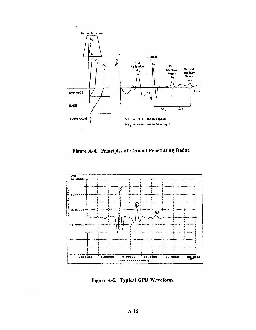
Radar Antenna
End Fleflectlon
Ao.
Surface Echo
A, First
ln1erflt.ce Return
SeC01\d Interface F;eturn
SURFACE
" • .. -0 >
SASE
SUBGRADE I J;. t, •.travel time in 2$proall
J;. t 2
.. travel time in b2$e layer
Figure A-4. Principles of Ground Penetrating Radar.
-18.8888 • • . . • . t
-•••~•• ' 4.••~•• •·••'•• ' 12.a~aa ' 1'·•••• 2e.eeae .. :ce
Figure A-5. Typical GPR Waveform.
A-16

In pavements, the parameter that most influences the dielectric properties of materials
is the moisture content. Table A-1 shows dielectrics for typical pavement materials. As can
be seen from this table, the addition of moisture to any of these materials will have a
significant influence on the dielectric properties of that layer. For example, a dry limestone
base course with 4% by weight of moisture will have a dielectric of around 6; if the
moisture content increases to 10%, then the dielectric of the layer would increase to around
11. The impact of a wet base on the trace shown in Figure A-5 would be to increase the
amplitude of peak B and to increase the travel time between peaks B and C.
The fact that GPR is sensitive only to changes in dielectric, which mostly equates to
changes in layer moisture content, is of major significance. Without these differences in
electrical properties, no energy will be reflected at interfaces. Several cases exist in
pavements where the layers are so similar electrically that no significant reflections will be
detected. Cases like this are common, such as granular base over sand subgrade, or concrete
over cement stabilized bases. In these cases, the electrical difference between layers may
not be sufficient to permit layer thickness estimates.
Table A-1. Typical Dielectrics for Highway Materials.
Material Dielectric Constant
Air 1
Water 81
Asphalt 3-6
Concrete 6 - 11
Limestone 4-8
Clays 5 - 40
Dry Sand 3 - 5
Saturated Sand 20 - 30
A-17
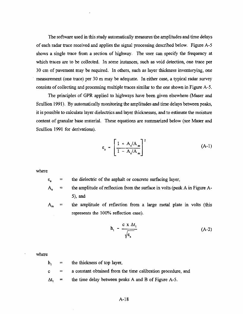
The software used in this study automatically measures the amplitudes and time delays
of each radar trace received and applies the signal processing described below. Figure A-5
shows a single trace from a section of highway. The user can specify the frequency at
which traces are to be collected. In some instances, such as void detection, one trace per
30 cm of pavement may be required. In others, such as layer thickness inventorying, one
measurement (one trace) per 30 m may be adequate. In either case, a typical radar survey
consists of collecting and processing multiple traces similar to the one shown in Figure A-5.
The principles of GPR applied to highways have been given elsewhere (Maser and
Scullion 1991 ). By automatically monitoring the amplitudes and time delays between peaks,
it is possible to calculate layer dielectrics and layer thicknesses, and to estimate the moisture
content of granular base material. These equations are summarized below (see Maser and
Scullion 1991 for derivations).
where
=
~ =
where
h, = c = At1 =
[ 1 + A IA ]
2
e = 0 m
a 1 - A/Am (A-1)
the dielectric of the asphalt or concrete surfacing layer,
the amplitude of reflection from the surface in volts (peak A in Figure A-
5), and
the amplitude of reflection from a large metal plate in volts (this
represents the 100% reflection case).
c x At1 h - --!
the thickness of top layer,
a constant obtained from the time calibration procedure, and
the time delay between peaks A and B of Figure A-5.
A-18
(A-2)

where
where
=
=
M =
I - [~]' + [~] I - [ ~:r -[ ~J
the dielectric of the base layer, and
(A-3)
the amplitude of reflection from the top of the base layer in volts (peak
B in Figure A-5).
M~ F. - 1 - y(f. - 1)
F. - 1 -y(f"s - 22.2)
the moisture content of base (% of total wt.),
(A-4)
e5 solids dielectric constant (varies from 4 to 8 depending on source
material), and
y dry density Yd (lbs/:ft3) divided by density of solids Ys (-165 lbs/ft3).
Note that equation A-4 assumes that the density along a highway remains constant.
This clearly is not the case and will limit the accuracy of moisture content estimation.
However, the moisture content is the major factor which influences measured base dielectric
constant i::b. The relative dielectric constants of air, dry granular base, and water are
approximately 1, 6, and 81, respectively. High base dielectrics are almost certainly
attributable to high moisture contents. The accuracy of equation A-4 is yet to be
determined.
A-19

The above equations serve as the basis for analysis of the data collected during this
study, as described below. They are based on the asswnption that the layer materials are
non-conductive and homogenous. This asswnption means that the imaginary component of
the dielectric constant tends to zero, and the mediwn does not attenuate the radar signal.
Therefore, all of the energy is either reflected or transmitted and none is lost in heating free
water in the layer. The asswnption of a very low imaginary dielectric from laboratory tests
at the Texas Transportation Institute appears to be reasonable for asphalt concrete hot mix.
However, it does not seem to be the case for either concrete or wet base course material.
Because of the higher attenuation, it is thought that the accuracy of layer thickness estimates
for both concrete layers and granular base layers may be less than for hot mix layers. The
layer thickness estimates for hot mix asphalts were found to be very good (Maser, Scullion,
and Briggs 1991). The accuracy on granular base courses was reasonable, but this was also
tied to the inability to physically measure the thickness of existing bases given the intrusion
of subgrade materials. The accuracy of these equations for measuring concrete thicknesses
is the subject of current research efforts.
A-20

APPENDIX B - CONSTRUCTION MONITORING DATA
SAN ANTONIO PAVEMENTS
In February 1992, H.B. Zachry was awarded the contract to overlay 14.75 km (9.167
miles) on IH-10 from the Kendall County line to 4 km (2.5 miles) north of Loop 1604 in
San Antonio. Two test sections were constructed: a control section and an experimental
section containing rubber-modified asphalt cement. The pavement depth was approximately
1.75 mm. By 1993, the new overlay failed, showing signs of alligator cracking, rutting, and
pumping of fine material. Right wheel path rut depths at four locations averaged between
0.8 - 14.7 mm (0.03 - 0.58 in.) with the deepest rut measurement being 27.7 mm (1.09 in.).
Following this failure, the outer lane of the overlay was milled, and the RAP material was
taken to Colorado Materials Company, where it was added to new aggregate and asphalt to
form a recycled CRM asphaltic concrete mix. The Roto-Mill was 4 m (13 ft.) wide x 64
mm (2.5 in.) deep.
On the original IH-10 job, a small size aggregate was used at the start of the job, but
by the end of the job, a larger limestone aggregate was in use, the gradation had been
changed from dense to gap-graded, and the binder content was increased to give the desired
film thickness. Because the coarser material gave better compaction and performance than
the dense graded material at the beginning of the original IH-10 job, the recycled mix design
used a coarse, gap-graded material.
Prior to laying down the recycled CRM mix as an inlay, an undersea! was placed
using a tack coat with precoated aggregate over the milled existing pavement. This undersea!
was later found to be unfavorable since it collected dust and did not particularly enhance
the milled surface texture, possibly reducing the potential for bonding with the surface
course. The inlay technique was potentially problematic since it had no outlet for stormwater
runoff. It was therefore important to maintain near zero permeability to prevent excess water
from ponding under the inlay and subsequently leading to stripping and freeze-thaw
destruction of the layers below.
B-1

CRM Mix Design
Control Mix (Original IH-10):
340 Type D asphaltic concrete with AC-20.
Experimental Mix (Original IH-10):
340 Type D asphaltic concrete containing a rubber-modified asphalt cement,
consisting of 82 % Fina AC-10 and 18% Tiregator Type II granulated vulcanized
rubber additive.
Final CRM Mix (Recycled IH-10):
30% CRM RAP, 5.7% asphalt, 79.6% aggregate (by weight) retained on the 2 mm
sieve. The following materials were incorporated in the CRM RAP Project:
1) Roto Mill - Item 3822 Plain Asphaltic Concrete Pavement (5 cm to 7.62 cm).
2) Seal Coat - Item 316 Aggr. (TY PF GR4).
Item 316 Asph (AC, HFRS-2P, CRS-2P or MC-2400 LTX.
3) Asphalt Item 3834 Asph. Concrete (Recycled Rubber) (Surf).
Table B-1 presents the laboratory results generated by the Materials and Test Division
verification of the mix design.
Table B-1. Verification of CRM Mix Design by TxDOT Division of Materials and Tests (IB-10--Bexar County, June 1992).
Asphalt Avg. Hveem Perm. Rubber Avg. Gr Ge Density VMA Stability Strain Binder Ga (cm/cm) (%)
6.5 2.242 2.369 2.596 94.6 20.9 1.3x10⁻³
7.0 2.292 2.350 2.592 97.5 19.6 48 0.5x10⁻³
7.5 2.263 2.345 2.606 96.5 21.0 38 0.3x10⁻³
8.0 2.257 2.342 2.623 96.4 21.6 32 0.6x10⁻³
8.5 2.231 2.301 2.587 96.9 23.0 1.0x10⁻³
B-2
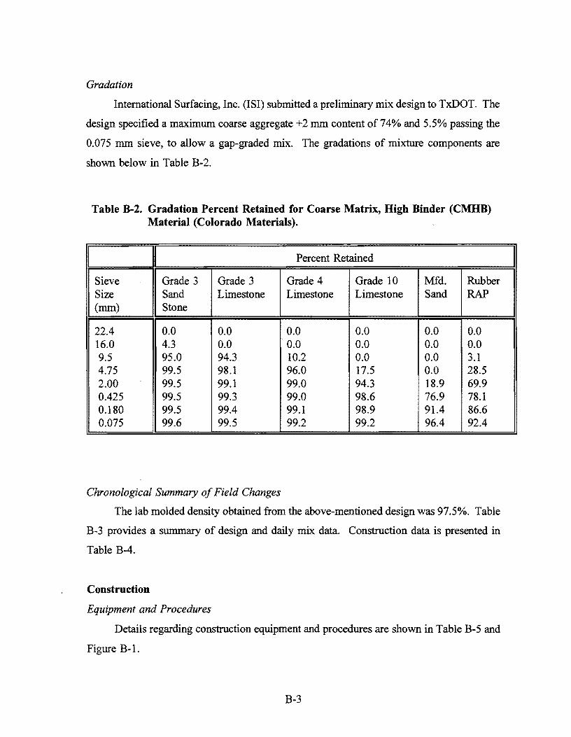
Gradation
International Surfacing, Inc. (ISI) submitted a preliminary mix design to TxDOT. The
design specified a maximum coarse aggregate +2 mm content of 74% and 5.5% passing the
0.075 mm sieve, to allow a gap-graded mix. The gradations of mixture components are
shown below in Table B-2.
Table B-2. Gradation Percent Retained for Coarse Matrix, High Binder (CMHB) Material (Colorado Materials).
Percent Retained
Sieve Grade 3 Grade 3 Grade 4 Grade 10 Mfd. Rubber Size Sand Limestone Limestone Limestone Sand RAP (mm) Stone
22.4 0.0 0.0 0.0 0.0 0.0 0.0 16.0 4.3 0.0 0.0 0.0 0.0 0.0 9.5 95.0 94.3 10.2 0.0 0.0 3.1 4.75 99.5 98.1 96.0 17.5 0.0 28.5 2.00 99.5 99.1 99.0 94.3 18.9 69.9 0.425 99.5 99.3 99.0 98.6 76.9 78.l 0.180 99.5 99.4 99.l 98.9 91.4 86.6 0.075 99.6 99.5 99.2 99.2 96.4 92.4
Chronological Summary of Field Changes
The lab molded density obtained from the above-mentioned design was 97.5%. Table
B-3 provides a summary of design and daily mix data. Construction data is presented in
Table B-4.
Construction
Equipment and Procedures
Details regarding construction equipment and procedures are shown in Table B-5 and
Figure B-1.

Table B-3. Daily Monitoring of Mix Properties for Recycled IH-10 Construction.
Date Ga Gr %2 Hveem %Air Total Creep Comp. Creep Permanent Recovery Slope of SS Y Intercept mm+ Stab Voids Strain (llkPa) Stiffness Strain Efficiency Curve (x 1000)
(kPa) (x 1000) (%) (l/s xlO')
10-4-93 2.374 2.414 79.2 38 1.657001 1.5 2.16xl0-5 46229.3 0.35 75.8 3 1.4
10-5-93 2.368 2.406 81.1 36 1.579385 1.3 1.84x10⁻⁵ 54489.3 0.33 73.8 2.4 1.2
10-5-93 2.372 2.418 77.1 27 1.902399 1.2 l.78x10-5 56254.3 0.43 64.9 3.8 I.I
10-6-93 2.353 2.416 80.2 35 2.607616 1.7 2.45x10⁻⁵ 40837.6 0.63 63.5 5.4 1.5
10-7-93 2.354 2.397 77.8 35 1.793909 2.2 2.98x10·5 33570.6 0.66 69.7 3.8 2.1
10-8-93 2.365 2.43 81. l 41 2.674897 1.4 2.0lxl0-5 49690.5 0.38 73 2.9 1.3
10-11-93 2.365 2.394 79 34 1.211362 2 2.18xl0-5 35549.4 0.53 73.5 4.1 1.9
10-12-93 2.379 2.395 77.7 35 0.668058 1.5 2.14x10⁻⁵ 46836.1 0.38 74.6 3.4 1.4
10-12-93 2.378 2.403 78.9 43 1.040366 1.5 2. IOxl0-5 47553.1 0.4 71.8 3.7 1.3
10-13-93 2.343 2.411 80.4 38 2.820406 1.7 2.54x10⁻⁵ 39327.7 0.51 70.8 4.9 1.6
10-14-93 2.355 2.414 82 40 2.444076 1.5 2.16x10⁻⁵ 46367.2 0.35 76.7 3.3 1.4
10-14-93 2.367 2.413 81 39 1.906341 1.3 l.96x10-4 50952.3 0.42 69.l 3.6 1.2
10-15-93 2.359 2.403 78.4 39 1.831045 1.4 2.03x10⁻⁵ 49304.4 0.38 71.6 3.2 1.2
10-15-93 2,362 2.412 80.6 40 2.072968 1.8 2.53x10⁻⁵ 39548.3 0.43 75.2 2.9 1.7

Table B-4. Daily Construction Data at End of Original IH-10 Job.
Date Sieve Size %Asphalt- Density Rice Ga VMA Avg.Core% Stiffness Strain Slope (1993) Rubber (%) (%) Air Voids (kPa) (l/sec)
9.5- 4.15- +2mm -.075 mm 4.15 mm 2mm
1115 37.7 32.3 70.0 6.1 6.8 97.2 2.370 2.304 19.0 11.4 - - -1115 - . - 7.3 - - - - 13.0 . - -7/16 39.2 31.9 71.1 6.6 7.9 98.5 2.339 2.304 20.0 13.0 . - -1111 39.7 33.4 73.1 6.5 1.1 98.2 2.338 2.296 20.1 . . . . 1111 39.7 33.4 73.1 6.5 7.2 96.7 2.356 2.278 20.3 . 19160.5 1.80 17.0 7120 43.7 33.7 77.4 6.2 1.1 98.2 2.346 2.304 19.8 6.8 - . -7/23 46.6 30.9 11.5 5.9 7.6 98.5 2.349 2.314 19.3 8.4 4467U 0.40 2.2 7124 42.0 34.9 76.9 4.9 7.6 98.1 2.356 2.311 19.4 12.0 45098.6 0.30 2.6 1125 47.6 28.1 76.2 5.6 1.1 98.1 2.357 2.312 19.5 9.3 52179.5 0.40 2.l 1121 45.0 32.I 77.1 5.1 8.1 91.1 2.349 2.295 20.4 9.3 44926.2 0.40 2.4 7128 44.4 33.2 77.8 3.9 7.3 98.9 2.355 2.329 18.6 8.7 49711.2 0.35 3.2 7131 46.2 29.7 15.9 5.3 8.l 98.4 2.352 2.314 19.8 - 48904.5 0.32 2.4 7131 49.5 29.4 78.9 5.0 1.1 96.9 2.383 2.309 19.6 - 44402.2 0.40 3.3 813 50.2 30.9 81.1 4.3 8.4 97.2 2.356 2.290 20.9 - 47546.2 0.46 2.5 816 47.8 32.3 80.l 6.3 8.7 98.7 2.331 2.301 20.8 5.3 34411.7 0.50 3.1 816 44.6 33.9 78.5 6.7 9.6 98.8 2.312 2.284 21.2 6.0 37652.3 0.60 3.5 816 - . - . 8.6 - - - . 8.8 . - -811 46.6 33.8 80.4 4.2 8.2 97.9 2.324 2.275 22.0 6.4 29316.5 0.80 8.1

Table B-5. Weights of Vibratory Roller
Two Wheel Vibratory Roller Caterpillar CB-614
Total Weight: 11,340 kg Front Wheel 5,466 kg Rear Wheel 5,874 kg
Dynamic Force per Drum:
High Amplitude 9,525 kg Low Amplitude 5,670 kg
Total Applied Force per Drum:
High Amplitude 15,195 kg Low Amplitude 11,567 kg
kg/linear cm at Front Drum:
Static 134 kg/cm Dynamic 233 kg/cm Total Applied 367 kg/cm
kg/linear cm at Rear Drum:
Static 144 kg/cm Dynamic 233 kg/cm Total Applied 377 kg/cm
Three Wheel Roller Ingram 12 ton EB
Total Unballasted Weight: 8,834 kg Rear Wheel Steer Wheel 5,985 kg
Compression: Rear Wheel 2,275 kPa Steer Wheel 986 kPa
Total Ballasted Weight: 11,754 kg Rear Wheel 8,014 kg Steer Wheel 3,741 kg
Compression: Rear Wheel 3,047 kPa Steer Wheel 1,289 kPa
B-6

Breakdown Roller: Smaller Roller: DD-10 DD-90 19.8-cm width 13.7-cm Diameter Amplitude 3
16.8-cm Width 12.2-cm Diameter Amplitude 3
Frequency 2500 VPM Frequency 1850-2600 VPM Force 83716 N Force 115742 N Weight 11612 kg Weight 9108 kg
1400
1300
......... , 200 E 0..
$ 3 Wheel
c: 1 1 00 :::> 0 u .... 1000 0
..!!:! 0 :::> .. Two Wheel z 900
800
700 0 2 4 2 4
Total Number Roller Posses
Figure B-1. Rolling Pattern Determinations for Recycled CRM Taken on October 6, 1993.
B-7

Problems Encountered and Solutions (Original CRM Job from Materials and Test Division
Records)
1) Difficulty with uniform compaction: Because the old existing pavement surface
had wheel path rutting depths of 1.87 to 2.5 cm (0. 75 to 1.0 in), uniform compaction was
very difficult to achieve. Personnel from Redland Stone Products recommended a flush coat
of emulsified asphalt be applied to the surface of the pavement in areas where inadequate
compaction yielded high air voids, to reduce excessively high water and air permeabilities.
2) Insufficient film thickness: The preliminary mix design offered by ISI produced
a somewhat tender and dry mix with low film thickness, causing placement and compaction
to be difficult. This was remedied by increasing binder contents from a low of 7 .2% to as
much as 8.5% towards the end of the job.
3) Shoving of mix under the roller: This was found to be caused by a low coarse
aggregate fraction (70% +2 mm material). The problem was alleviated by cutting the
discharge temperature of the paver from 149° to 138°C (300° to 280°F), and increasing the
+2 mm fraction from 70% to 74%.
4) Substitution of Coastal AC-10 for Fina AC-10: At station number 392+94, Coastal
AC-10 replaced Fina AC-10 because Fina was unable to produce any more AC-10 which
would meet specifications.
5) Low road densities: This problem was addressed by varying mix temperature,
asphalt content, and gradation, as well as continuously reminding the contractor about the
rollers keeping up with the laydown machine.
ENVIRONMENTAL MONITORING
On June 17, 1992, a pretest meeting was held in Austin to discuss an air pollutant
emissions test program to be conducted by Southwestern Labs, Inc.. Representatives of
TxDOT, the Texas Air Control Board, Redland Stone, the H.B. Zachry Company, and
International Surfacing, Inc. attended the meeting. It was determined to test several
parameters of the emissions under three operating conditions in the baghouse stack of
Redland Stone Products Company, producer of the mix. Results are shown in Tables B-6
and B-7.
B-8

Table B~6. Summary of Findings from Stack Monitoring.
Temp Percent Plant Rubber
H 0 D H 0 D H 0 D L 18 D L 18 D L 18 D H 18 D H 18 D H 18 D
H 0 R H 0 R H 0 R L 18 R L 18 R L 18 R H 18 R H 18 R H 18 R
H 0 c H 0 c H 0 c H 18 c H 18 c
18 c
H =High Temperature (163°C) L =Low Temperature (149°C)
voe Benzene
9.0196e-OS 6.8303e-07 l.083le-04 2.7806e-03 8.3103e-OS 2.313le-03 l.140le-04 3.5029e-03 I.I 189e-04 2.7813e-03 1.1461e-04 l.1636e-04 5.1968e-OS 9.9153e-04 8.6278e-05 2.7768e-03
2.7146e-05 2.0361e-04 3.4492e-05 2.2194e-04 3.1544e-05 l.5665e-04 3.4363e-05 l.6361e-04 6.7639e-06 l.2429e-04 7.3330e-06 l.2800e-04 l.9086e-04 l.5303e-04 1.2372e-04 l.0245e-04
t.1744e-05 l.8187e-04 2.0210e-06 6.6408e-05 2.0161e-06 l.4432e-04 4.6316e-06 3.3172e-04 3.6775e-06 2.2340e-04 4.2405e-06 3.5306e-04
D = Duininck Bros;
Emission Rate (kg/kg mix)
Styrene Naphthalene 2-Methyl-naphthalene
l.S774e-10 S.142Se-07 8.8337e-07 l.2323e-06 4.0130e-07 6.4303e-07 l.2386e-07 3.S2S2e-07 S.716Se-07 l.2Sl7e-07 2.56S3e-07 4.9296e-07 6.9164e-08 2.51 IOe-07 5.7889e-07 2.7912e-07 4.9989e-07 6.l 185e-07
3.4395e-07 1.0617e-06 4.8747e-08 l.8555e-07 5.9912e-07 l.0633e-07 2.6969e-07 6.0409e-07
-1.6422e+OI 2.4314e-07 l.2183e-06 9.0533e-09 4.0222e-07 l.8365e-06 8.0184e-09 4.0868e-07 1.8106e-06 2.5866e-09 3.4919e-07 l.7330e-06
2.7289e-07 l.4226e-06 2.9617e-07 l.S908e-06
2.2762e-08 4.5524e-07 2.0951e-06 2.8116e-07 3.8540e-07 l.7847e-06 2.6125e-08 3.0651e-07 l.6554e-06
l.9915e-08 5.2416e-09 l.3473e-08 7.5604e-09 l.0282e-08 2.9666e-09 2.5163e-08 l.0603e-08 2.5673e-09 3.0428e-08 l.5915e-08 2.1299e-08 1.963 le-08 l.7477e-08
R = Redland Stone; C Colorado Materials
Phenanthrene Butadiene Particulates Opacity (% / 907 kg)
l.8929e-08 4.8900e-07 2.33S6e-OS 4.6604e-02 4.8978e-08 4.1868e-07 3.0987e-OS 6.1832e-02 4.9226e-08 4.79S6e-07 2.6212e-05 S.2304e-02
4.6824e-07 2.3548e-05 4.6987e-02 3.8643e-07 2.7984e-OS 5.5839e-02
9.4618e-09 6.9228e-07 2.7707e-05 5.5286e-02 7.6957e-08 5.2141e-07 8.2080e-05 1.6378e-01
4.3558e-07 l.8266e-OS 3.6448e-02 3.9297e-07 3.4544e-OS 6.8930e-02
l.4718e-06 3.4027e-05 5.1097e-02 1.8106e-07 7.6951e-07 5.1370e-05 4.2581e-02 1.7977e-07 7.6563e-07 7.4313e-05 5.2129e-02
5.3413e-07 l.8261e-05 4.8516e-02 8.6134e-07 9.8549e-06 5.4968e-02 9.4023e-07 l.0799e-05 5.0065e-02
2.3280e-07 l.8986e-06 l.3528e-05 5.9613e-02 2.0046e-07 5.1732e-07 l.3256e-05 6.1419e-02 2.0305e-07 l.4912e-06 l.1860e-05 7.8452e-02
7.7228e-JO l.298le-07 l.1347e-07 9.4340e-03 2.3617e-09 l.1809e-07 6.2439e-07 l.2459e-02
l.4771e-07 3.6482e-07 1.2579e-02 l.7760e-09 1.7603e-07 2.9309e-06 2.1661e-03
l.9621e-07 1.2619e-06 2.1583e-03 l.6599e-07 1.1840e-06 4.3956e-03

Table B-7. Statistical Analysis of Air Emissions Data.
Conventional HMA (Oo/•) Modified HMA (18%)
Mean Standard Mean Standard Modified: Error Dev. Conventional
HMA
voe 0.009242 0.007338 0.008462 0.008347 0.000781 0.023434 0.004033 0.004023 0.010497 0.009148 1.2575
Benzene 0.000332 0.000223 0.000353 0.000303 0.000057 0.000182 0.000066 0.000144 0.000131 0.000048 0.432291
Styrene 0.000061 0.000043 0.000039 0.000047 0.000009 0.00004 0.000015 0.00005 0.000035 0.000015 0.737662
Naphthalene 0.000032 0.000035 0.000033 0.000002 0.00001 0.000021 0.000021 0.000017 0.000005 0.521635
2-Methyl- 0.000027 0.000006 0.000005 0.000013 0.00001 naphthalene
0.000002 0.000005 0.000004 0.000003 0.000001
Butadiene 0.000351 0.000392 0.000331 0.000358 0.000025 0.000259 0.000236 0.000295 0.000263 0.000024 0.735021
Particulates 0.005848 0.002S18 0.002363 0.003576 0.001608 0.000226 0.001246 0.000728 0.000733 0.000416 0.205079
to I -0

PERFORMANCE
Rut depth measurements taken prior to recycling are shown below in Table B-8.
Table B-8. Rut Depths Measured in Wheel Path of Original lli-10 CRM Overlay (8 Oct. 1993, Prior to CRM RAP Recycle).
Location Distance LRUT RRUT
(m) (ft) (mm) (mm)
TP4 0 0 0 1.5875 TP4 3.05 10 0 6.35 TP4 6.10 20 1.5875 12.7 TP4 9.15 30 6.35 14.2875 TP4 12.20 40 6.35 19.5 TP4 15.25 50 0 6.35 TP4 18.30 60 0 6.35 TP4 21.35 70 0 11.1125 TP4 24.40 80 0 12.7 TP4 27.45 90 0 12.7 TP4 30.50 100 1.5875 9.525 TP4 33.55 110 0 15.875 TP4 36.60 120 1.5875 6.35 TP4 39.65 130 0 9.525 TP4 42.70 140 1.5875 9.525 TP4 45.75 150 1.5875 17.4625
TP5 0 0 0 7.9375 TP5 3.05 IO 0 7.9375 TP5 6.10 20 0 7.9375 TP5 9.15 30 0 7.9375 TP5 12.20 40 0 7.9375 TP5 15.25 50 0 7.9375 TP5 18.30 60 0 7.9375 TP5 21.35 70 0 7.9375 TP5 24.40 80 0 7.9375 TP5 27.45 90 0 7.9375 TP5 30.50 100 0 7.9375 TP5 33.55 110 0 7.9375 TP5 36.60 ' 120 0 7.9375 TP5 39.65 130 0 7.9375 TP5 42.70 140 0 7.9375 TP5 45.75 150 0 7.9375
B-11

Table B-8. (Cont.)
Location Distance LRUT RRUT
TP6 0 0 (mm)
3.175 (mm)
3.96875 TP6 3.05 10 3.175 2.38125 TP6 6.10 20 3.96875 0 TP6 9.15 30 4.7625 3.96875 TP6 12.20 40 3.96875 3.175 TP6 15.25 50 2.38125 2.38125 TP6 18.30 60 3.175 3.96875 TP6 21.35 70 3.175 3.175 TP6 24.40 80 2.38125 2.38125 TP6 27.45 90 3.175 0.79375 TP6 30.50 100 3.175 0.79375 TP6 33.55 110 0.79375 3.175 TP6 36.60 120 0.79375 1.5875 TP6 39.65 130 1.5875 1.5875 TP6 42.70 140 2.38125 3.175 TP6 45.75 150 3.175 3.175
TP7 0 0 1.5875 3.175 TP7 3.05 10 17.4625 3.175 TP7 6.10 20 9.525 14.3875 TP7 9.15 30 10.31875 27.78125 TP7 12.2 40 15.08125 19.05 TP7 15.25 50 26.19375 11.1125 TP7 18.3 60 7.9375 5.55625 TP7 21.35 70 7.14375 7.14375 TP7 24:40 80 16.66875 12.7 TP7 27.45 90 17.4625 14.2875 TP7 30.50 100 11.90625 19.05 TP7 33.55 110 18.25625 19.05 TP7 36.6 120 18.25625 22.225 TP7 39.65 130 16.66875 14.2875 TP7 42.70 140 3.96875 23.8125 TP7 45.75 150 11.1125 17.4625
B-12

LABORATORY STUDIES
Rheological data for CRM and control binders are shown in Tables B-9a through B-
9e.
Binder
Table B-9a. Binder Viscosity Data, 25°C, 0.1 Rad/sec, 5% Strain.
v........,. Dala
~ionc: 25 C:.lslus, 0.1 radls.c, 5% strain Glop: 5DO ................. II'!(, -·
1000 -- lat $'!(, - 10'1. 40 - -1500 ............ lat 1$%, 111"l(.. - 20ll. 40 - --
1500 ....,_,at$'!(, - 10'!r. 10 - -2000 mic7Dns tor 1$%.. 18"lf.. and 20ll. 10 - -.
Noto: TG • T ... Gae< - TJ?O. RS•~ A.- TJ?O
ABM-1 -Tn>O ~ -Con!---~ "-1iHllJnilsl 0%1 5% 10% 15%( ,.G.1omes11 Visc:asity (poise) ,2•13000~ 4052000 5508000 51>610001
d("-l 86.7 711.32 6<1.P4 59.13 G•lsift(al <~cm•21 2•1700.802 •137117.764 608038.078 604485.52
,.G·40- V-11J*MJ :14130001 3027000 •18•000 51118000 11(~1 86.7 77.2• 68.31 61.28
a•111infil) 1e1yne1cm•2l 241700.802 31036'.916 •50281.401 591576.1>52 Rs.40mesll v.....,;iy tpoial 2'1300;1 3464000 3535000 2853000
il~I 86.7 75.'7 611.28 61.51 a·•sinlil\ 1~cm·21 241700.802 357845.27' 380515.42$ 324610.328
ABL-2 -T,;ie ~ -Con!---~ ..._,,... !Unl!•l II'!(, 5%1 1""' 15%
,.G·10- v.......ay (poiM)
!::~:~~~ 7750001 1635000 3688000 did-I 71.01> 51.32 50.3
G•11inlil) fdyneicm'2l 308 0
81921.4246 19•2•0.1197 '7fl335.11P
TG. '° -1 VISCOSily jp<IOM) I 30•100 730500 161>1>000 30630001 i(d-1 80.21 70.~I 60.7• 51.llS
a·•slftlil) 1~cm·21 30859.31>33 77296.456 194747.121 38811'5.857
l'IS-40- V-y (poiM) :1041001 63'6001 12420001 23820001 d(d-) 80.21 1•.•2 M.•8 53.58
a•1sinCil) fd.,,...cm':Zl 30851>.3033 65880.7155 137627.1' 2"016.0!IS
DIAMOND SHAMROCK AC-5 -Trpe ~ -eoni.... --Site "'-lie• llJnilSI 0'1o 10% 15%
TG.· 10- V-1 fpOiael 436100 8130001 11360001 d(d-) 8'.H 71.•6 65.1>2
a•ISin!il) (C1r'*cm•21 Y0•0.7512 50.306<& 102521 .833
TG·40-, V-r~) •:16100 8610001 0070001 •1"-l 81 .118 t50.02 65.12
G.·1smrai 1-c:m·21 .U0•0.7512 !02213.2695 99978.91184
MADE AC-5 -Trpe1~ -c-.... .....,.._,sc.., "-iec l\JMSI
°""' 5% 10% 15%1 TG.·10- V~(poiMJ 5721>00i 1'00000 1517000 1$1>8000
a(~I 89.01 I 72.llS 61> 51>.H G•Jainlal 1e1r'*cm•21 51298.5545 1360•1> ""' 1624112.751> 18453!0.830
TG·<&Q- v ........ , (poiM)
smo~I a:i::~: 020000 1!1 6000 ii~) 80.01 70.117 64.01
G•1,.;m<!) 1e1..-cm•21 5721>8.SS•S 6•SS3. 1>7311.6K7 1011105.711
YBF, AC-20 I I
18% 6385000
5'.PS 7617!>6.367
3808000 55.76
<&60633.551 4586000
55.18 558621.•65
1""" 4P'8000
··~•9 703934.518
3825000 46.05
S312P0.31>• 3463000
•6.81 '"'sn.2os
20% 1305000
SS.71 151132.075
l>OJOOO 51>.37
105523.121
20% 1658000
53.•2 206469.268
856000 SfUP
91>665.832
I 20%1
TG. "° _, y,._.,, tpo.MJ I 1&2•0001 7641000
1 760SOoo~I
i ,.,_, 8'.117 68.5£ 62.76 G·1sin<ol '"-'cm•21 183133.583 820!IOIU1' 855362.605
62:100001 51 500001 57.711 51 .H
736•0o a:i es• 776 , es
B-13

Table B-9b. Binder Viscosity Data, 25°C, 0.9796 Rad/sec, 5% Strain.
v-.,.Dca Condlians: 25 C.ls!us,
G.,: 0.9796 radlsec, 5% strain
500 - .... C% -· 1000 micrDM IOf $% - lD'X. 40 IMSh-. 1!i00 rnlcrcns tor 15%. 1!'11.. and 20'1. 40 lllHb -· 1500 micnlnslOt 5% an<l 1D'X. 10 - -.
2!)00 - '"' 15%. 111%. - 20'l(, 10 - -· Noto: TG • T .. Galer R.ct- Tr,>o. RS • - ,,._ TJl>O
ABM·1 -Typt ~ R\lt>bet Ccntltftl --Sl:e -iooslUnilsl 0% 5% 10% 15% TG-10,,_,. V"""'5ily (l>OiNJ 2395000 29•5000 )004000 2676000 .,._, 7i.48 73.89 62.33 58.07
G"l$lnrai 1e1y.,..,em·2l 2403291.93 30028•2.~1 332271 S.S3 3088755.52 TG·.&O,,_,. v_, (poisel 23QSOOO 2111000 2321000 237•000
·•(ffV'MI 77.•8 69.Sl 61 .81 57.37 G"lsil\faJ fdy-em•21 24032;1.93 226•208.59 2579633.59 276U03.•7
Rs..&0- v_, (l>odel 2395000 2377000 2016000 13$13000 i(d-l 77.•8 75«7 63.48 62.1.t
G"ISi..iil ldr_,.,,,,.2l 2C0:!291 .Si') 240$44.C .63 2207109.81 15<13•85.66
ABL·2 "-Typo ~ I R-C-ent --&r.. "'-ies tun1111 I 0"41 5% 10% 15%1 TG·10,,_,. v-r IJ>OiSel I 2165001 •20000 &'8000 12150001
•i~l 74.28 64.2 5•.28 '7.67 G"Jsirl!a\ tdr...,cm•2) 22032•.201 •56985.016 78\1165.959 1609967 .82
TG·<IO- V-ylJ>OiMI 216500 3P<OOO 706000 '0•200:1
i(~l 7'.28 63.83 S.t.<3 •7.911 G"'lsinCC) ld'f'1\elcm•21 22032•.201 <300•6.ll• 850250.018 1373762.2<1
RS-40- Viscos.lly (paiMI 216500 3611000 ~9000 8270001
··~) 74.:;!B 65.P3 ss .. 11 •S.65 G"'Jsinfa") ld.,.-em•2i 22032 .. 201 395896.618 5•5007 .775 1079183,14
DIAMOND SHAMROCK AC-5 -TJ!>O ~ -e--•nc!-S... -iesnJ-\ 0 ... 5% 10...f is% TG·10- V-ylJ>OiH) n•3oo 341000 <230001 •20000
•1~1 76.89 71.3 $6.36 60.0 G"lsint11) (dyn41:1c:m•21 326185.~6 35U60.573 •52329.072 •no .. •.6•7
TG·<IO- V&S<:DSity (.pO<M) 32<300 413000 •3•0001 '12000 .,._, 76.11!1 70.12 65.07 61.33 G"/Sin(i!) (Gy-c:m•21 326185.P•6 t.3C2'12.664 •&8830.615 •S991l1.515
MADE AC·5 _T,,,_1~ Ruot>ef Comem
--- -;,,,, nJnllsl 0% 5%1 10% 15%1
TG • 10 -, V""°""l' (pc.NJ 55$.400 8160001 88•000 73&8001 • 1o.or-i 85.23 70.'8 68.•8 61.3$1
G"tsinla\ tovnoJcm•2J ~•5960.813 8•8098.•25 noes7. 1112 82•386.1169
TG·..0-1 V-y (-l SH•ool 6220001 ssiooo 47200~1 •1--1 SS.23 76.!5 70,15 6".llS
G"'ISinfa"I lO,..nel'cm•21 S45060,813 626•9•.0'8 564270.3'1 S10371L2B3
YBF, AC-20 _r,,,. ,~ Ruct>e-t Com4f'l'\1
""" - Sin .._ ... IUMsl O':. 5% '°"' 1$%
TG·~-1 v...,.,.,.,(_I , .. , , 000 3969000 .3493000 2657000 acd_..1 75.;2 52.88 51.23 ~1.::!i
G'"Jsmt.11 fdVMJcm ... 21 "2S02S.12 •876053.15 •3&&7:!i .9a 33346,•.98
B-14
18% 2832000
57.72 ne136t.ta
162:)000 S6.~
18H019.S9 1887000
SS.~4
22.&'1311 .23
18%
1"8•000 44.02
2091966.7 1183000
•5.61 1621712.88
1061000 •<.72
1477107.88
20% 503000
~s
601523.3•7 363000
57 .6" •201171.037
20% 6•5000
5S.1S 769928.3•9
;)8&000 &0.2
'3S'l'•6.S38
20% insooo
5""2 2"2228.47

Table B-9c. Binder Viscosity Data, 60°C, 0.1 Radlsec, 5°/o Strain.
v-,.o.. Condil....., 6tJ Calslus, O. i l"llcl/s•c:, S% stniln
Go;>: 500 - 1 ... C'4 rubber. 1000 mic:ronS lor 5% and 10% ~ - -. 1500 mic:ronS lar 15'r.. 111'X.. anct zp% ~ _,, -.
1500 "'"""""'"' 5% - 107. 10 ... - --2000 - lar 15"1.. 1n:., - 2P% 10 - -
No••: TG • Tn Golor ~ TYPll. RS• Ac.a. -T\'P9
ABM-1
TG • 10 ,,_ V-.lly (l>aiMI
il !.S.V-! G"Jsinfa) ! cm•2)
TG • 4ll ,_ VGCOOity !J>Cdel 'i!d-)
G "/sinl a) I e1,_ic:m•21 RS- 4ll ...-. v........iry (poise)
il!~I G"Jsinla) 10yno.1cm•21
0%
211)21 80.U
219.200164 211l2 81l.93
210.200164 21;2 Bil.SJ
2H.20016'
5'11. 57118
86.28 581.024248
5302 86.38 83.55
531.26004 llBS.ll4088 5880 ll776
88.34 M.08 S88.2•681l3 982.8'1743
ABL-2
TG • 10 ,_ V........ay (poise)
TG-~..-.
ilC6-l G"/sin(a) fClyM/Cm'
Vis<>ooity (j>oise) I 11(6-1
G"Jsl!\lal '""""""'•2i v........ay (poise!
11(6-l G"lslnla) (11yM1<::m•21
'44.6768011 1221 3205
111.86 811.41 122.100365 320.516"8
DIAMOND SHAMROCK AC-5 R.-TYPll ~ I R-Conlem ~MesnSi:r• P""""'iff l\.lnllsl I 0% 5'11. 10'11. TG-10.-
v.....iiy (paiMJ I 7Z3.8 161l1 2570 il(CI-) H.H 81.114 113.42
G"lsin!O! IC!yMl='2l 72.3801336 170.787101 258.704166 TG-40,,_
Visc:cclly (poMI I 72.l.8 2138i 31621
a'""""'"'' H.89 86.68 11:2.511 G"Jsinlll) lclvM'Cm'2l 72.3801336 214.15114•8 318.162981
MADE AC-5
TG • 10 ,_ V-1 (poMI 88•.8 il~l 90.08
G"laiftfll) l-Cftl·2l H.•800861 TG • V.._, i-1 804.8
i ,.,.._, 90.08 G•Ja.JnC~ ht,.,n9icm•2\ 68.•8008&1
YBF, AC-20 R-T-~ -c----Sii• "-"'" tvnilsl o...I 5%1 '°"" TG-41l,,,_ V-y(-1 26Hj 161461 30660
il (Cl"9'MI 8Q.88 12.7• 76.11 G'lsinfal IC1v,,.,cm•2J 2U.80DSQ2 1s21.r..;211 3157.5'03•
B-15
15 ... 3721)0 H.72
4318.115'5 18180 i7.35
•863.22843 21850 67.53
236-t.5154'
15% 508PO 68.59
5466.21385
15% 4575 71.5
482.430401 5473
72.75 573.077228
15'!0;l ... ,,0, 67.2$
•139.17998
18% 60070 54.5
7373.117674
'7550 55.4
5776.68885 37530 64.49
4158.40395
18% 114200
'1.4 13007.0923
100500
68.39
20'11. 111170 60.18
137S.681SP 10300 64.27
11'3.36533
20% 47,80 "l!.02
6387.0512 24810 SI.OS
3100.'l99
2ll'll.
702110 58.011
8279.15'11

Table B-9d. Binder Viscosity Data, 60°C, 1.0 Rad/sec, 5o/o Strain.
V-,.Dma Condllionc 60 C.lslus, 1 .0 r.adlsec, S% strain
~ soo...-1 .... 0%..-. 1000 ......_ lor $%and 10% •O mun-· 1500-.... lor 15'1(.. 1e'J.. and= 40......,, --
1500 micronS tor$% and 10% 1D - -· 2000 .....,_. lor 1$%. 111%. and 20'r. 10 .._11 -.
Nole: TG • Tn Golar - Tr;H. AS• """'- -T!'P'
ABM-1 AubbetTr;:>e ~ Flubbe< Comenl
and_, Size Prooet1"'11 f\Jnilsl °"" 5% 10% 15%
TG • 10 -, v_, (poiM) UDll '10125 ,.6201 111150 i(devrM) 85.7• '":es 67.03
G"lsin(il) lcl,.,..,cm•21 •'38.6<'78 16372.1111 20799. 11101
TG·"'O- V-y (poiM) ·•312 7811' 13•50
ild-1 81.S1 77.77 G"/siftfi) (dv...,cm•21 79ES.23796 13762.3381
AS-40mosn Viscm:ily (l>OiMJ 7371 1211601 ilcl-J 81.93 65.03
ci·1sinl0l ld,.,..,cm' 7U•.72'15 13879.::ZS68
ABL-2 -T- Rhoolopical Rubi* Cantenl --Size """"""""' llJnll•l °"" 5% 10 ... 15%1
TG·1D- v-r~I 1211 306 130•0 ::Zll750l i(d-) H.6 8•.12 59.73 65.::ZB
G"lsinlOJ fclV"•IC:,,.•21 1::Z11.36164 3514.491•6 15098.5•89 ::12751.2651
TG·"°- v..-., (pOiM) 1211 321131
86>2 226101 il"-l 88.6 83.311 75.65 70.57
G"lsinlil fC!_..,.,.,...•21 1211.361&4 331~.03654 8835.77191> 23Si~_,.t31
RS-411- v..-., IPoial I 12111 2656 60901
1700:1 ild-J 88.6 86.ll8 82.81 73.ll6 G"Jsinlil 1.,...,,.,cm•z1 1211.'616< 265Uill31l5 6138.2688• 17688.64'3
DIAMOND SHAMROCK AC-5 A.-Tr;:ie ~
and""""" Size p....,.., ... !Unitsl
TG·10- v.......,, l)x>iaMtl .,.,_, G•1sintal (ttyneilcm"'2'1
TG·'ll..-i V-y (Poial I il~I
G"Jsineil'I id,.,..,cm"2l
l'l-T-1~ ..... -Sil:• """"""'" tunOsl TG • 'll -1 V..._.,y tpas<t)
••o~•l G•Jsin!il fctY"-'cm•2J
Rubi* Coruent
0%1 5%1 10%1 15%1
726.•1 1189~ 181'1 305:1 H.35 llS.11 8•.06 77 .ei 726.4'67S8 11$2.05082 1$23.711252 3127.~176•
726.41 16041 23'11 358Dt H.35 85.113 82.27 76.4'7
726.•.&67511 1608.055$3 2362.•6635 3662. 19077
MADE AC-5
15%
100801 62.3
11384.712~
6373 66.•6
US1.•P599
YBF, AC-20
15 ... 25280 66.7-'
27!'16 C87S
B-16
U!%
26•70 62.38
2987•.•513 21'80 61.311
24469.8375 21180 67.03
::Z3004.D128
1e.._
53<20 57.211
63•8S.213.& .C2720 55.12
52075.2653 35•00 62.58
398110.391\)
2trl'.
Sll•O 70.711
6-184.72957
5111>• 6P.2S
6302.83<31
20%
16610 55.2•
202'711552 Si814
59.25 -:icis.si ss
20 ... 338110 60.81
:i&e1s ess1
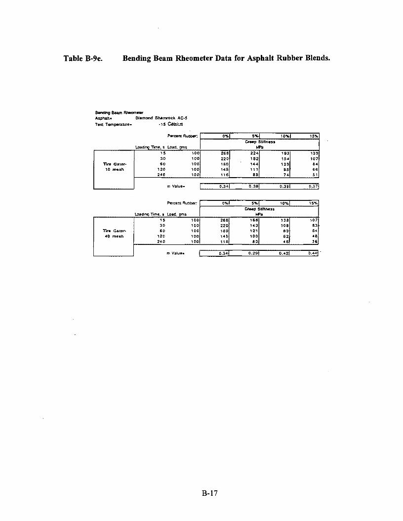
Table B-9e. Bending Beam Rheometer Data for Asphalt Rubber Blends.
Banding Beam Ri'leom•l81' Asphan• Diamond St..mrock AC·S
Test TemperallJ:r&- ·15 Celsius
Percern Au:3ber: O'Y. 5% 10% 15"4 Cree;:> Silliness
t.oadina Time. s Lead. 9"'S M"a 15 100 2Ei8 224 193 133 30 100 220 182 154 107
Tir• Gator• 60 100 180 144 123 84 10 mesh 120 100 145 111 FIS 66
240 100 116 es 74 51
m va,ue. I 0.341 0.38j 0.381 0.37j
Percent Ft1.o-:t.>er: 0%! 5"4 10% 1S"4
Creep Silliness L.oadinc:l nme. s Ll>ad. i;ims .......
is 100 26S 166 138 107 30 100 220 143 108 83
Tire Gator• 60 100 ieo 121 83 64 40 mesh 120 100 HS 100 62 48
240 100 116 80 46 36
m V•lu&- I 0.341 0.29. 0.1.21 0.44l
B-17
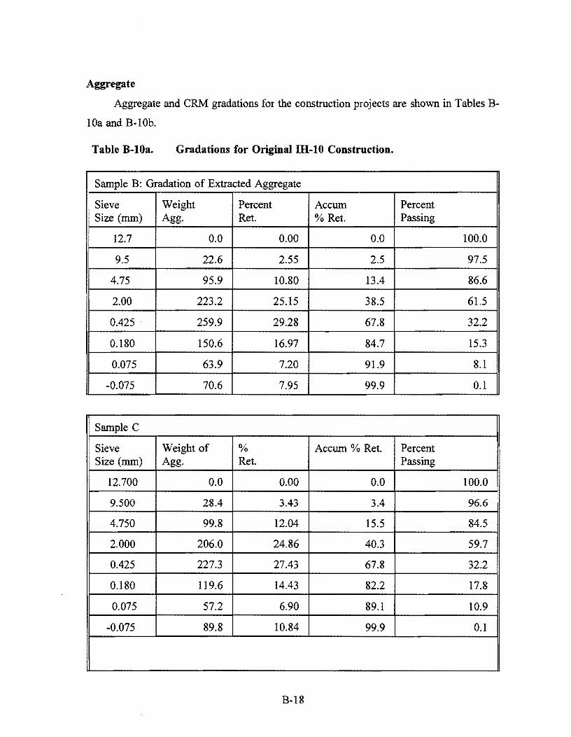
Aggregate
Aggregate and CRM gradations for the construction projects are shown in Tables B
lOa and B-lOb.
Table B-lOa. Gradations for Original lli-10 Construction.
Sample B: Gradation of Extracted Aggregate
Sieve Weight Percent A cc um Percent Size (mm) Agg. Ret. % Ret. Passing
12.7 0.0 0.00 0.0 10
9.5 22.6 2.55 2.5 97.5
4.75 95.9 10.80 13.4 86.6
2.00 223.2 25.15 38.5 61.5
0.425 259.9 29.28 67.8 32.2
0.180 150.6 16.97 84.7 15.3
0.075 63.9 7.20 91.9 8.1
-0.075 70.6 7.95 99.9 0.1
Sample C
Sieve Weight of % Accum % Ret. Percent Size (mm) Agg. Ret. Passing
12.700 0.0 0.00 0.0 100.0
9.500 28.4 3.43 3.4 96.6
4.750 99.8 12.04 15.5 84.5
2.000 206.0 24.86 40.3 59.7
0.425 227.3 27.43 67.8 32.2
0.180 119.6 14.43 82.2 17.8
0.075 57.2 6.90 89.1 10.9
-0.075 89.8 10.84 99.9 0.1
B-18
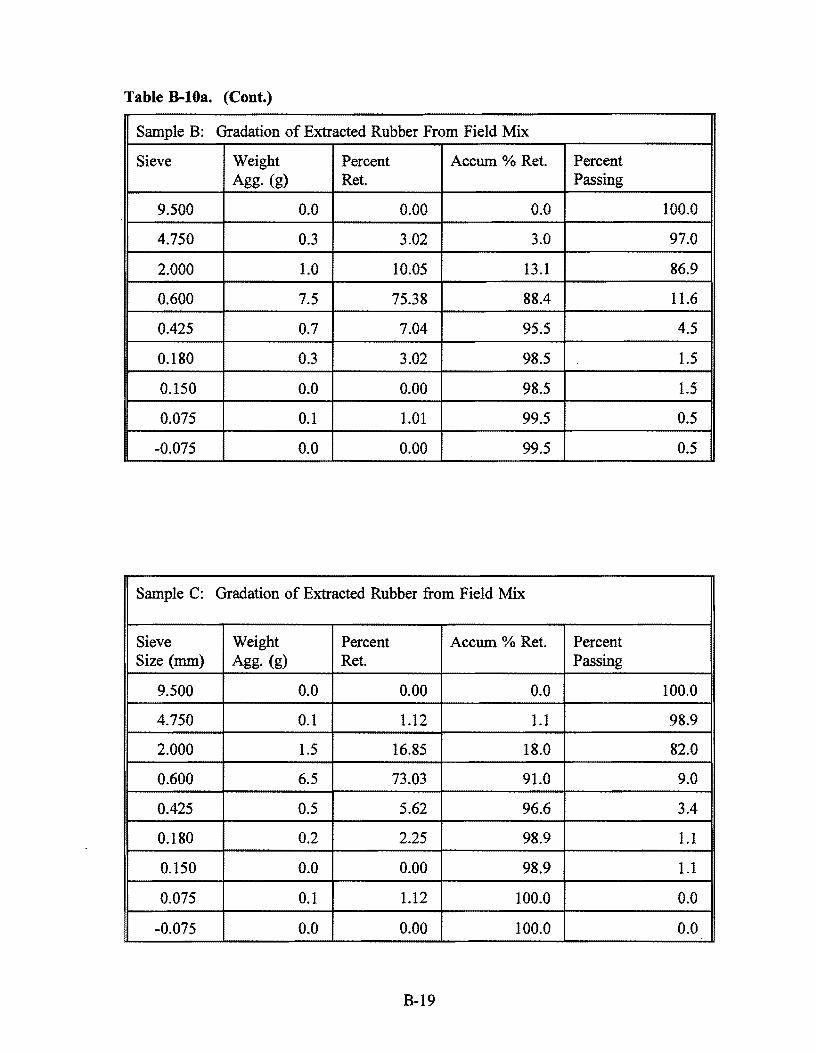
Table B-lOa. (Cont.)
Sample B: Gradation of Extracted Rubber From Field Mix
Sieve Weight Percent Accum % Ret. Percent Agg. (g) Ret. Passing
9.500 0.0 0.00 0.0 100.0
4.750 0.3 3.02 3.0 97.0
2.000 1.0 10.05 13.l 86.9
0.600 7.5 75.38 88.4 11.6
0.425 0.7 7.04 95.5 4.5
0.180 0.3 3.02 98.5 1.5
0.150 0.0 0.00 98.5 1.5
0.075 0.1 1.01 99.5 0.5
-0.075 0.0 0.00 99.5 0.5
Sample C: Gradation of Extracted Rubber from Field Mix
Sieve Weight Percent Accum % Ret. Percent Size (mm) Agg. (g) Ret. Passing
9.500 0.0 0.00 0.0 100.0
4.750 0.1 1.12 1.1 98.9
2.000 1.5 16.85 18.0 82.0
0.600 6.5 73.03 91.0 9.0
0.425 0.5 5.62 96.6 3.4
0.180 0.2 2.25 98.9 1.1
0.150 0.0 0.00 98.9 1.1
0.075 0.1 1.12 100.0 0.0
-0.075 0.0 0.00 100.0 0.0
B-19

Table B-lOa. (Cont.)
Gradation of New Rubber • (never been extracted)
Sieve Weight of Percent Cumulative % % Size (mm) Aggr. (g) Retained Retained Passing
9.500 0.0 0.00 0.0 100.0
4.750 0.0 0.00 0.0 100.0
2.000 0.0 0.27 03 99.7
0.600 5.5 50.00 50.3 49.7
0.425 2.4 21.82 72.1 27.9
0.180 2.3 20.91 93.0 7.0
0.150 0.1 0.91 93.9 6.1
0.075 0.5 4.55 98.5 1.5
-0.075 0.1 0.91 99.4 0.6
B-20

Table B-lOb. Gradations for Tyler CRM Job.
DATE 10-15-92 l\1ECHANICAL ANALYSIS OF EXTRACTED AGGREGATE
SAMPLE NO. 1
Sieve Size Wt. of % Retained Accum % Passing (mm) Aggregate (g) %Retained
12.700 0 0.00 0.00 100.00
! 9.500 65.8 6.98 6.98 93.02
4.750 367.5 38.97 45.95 54.05
2.000 227.6 24.14 70.08 29.92
0.425 128.3 13.61 83.69 16.31
0.180 51.8 5.49 89.18 10.82
0.075 66.9 7.09 96.28 3.72
-0.075 31 3.29 99.57 0.43
DATE 10-15-92
l\1ECHANICAL ANALYSIS OF EXTRACTED AGGREGATE
SAMPLE NO. 2 I
Sieve Wt. of % Retained Accum. % % Passing Size (mm) Aggregate (g) Retained
12.700 0 0.00 0.00 100.00
9.500 58.9 6.25 6.25 93.75 i 4.750 373.1 39.57 45.82 54.18
2.000 229.8 24.37 70.19 29.81 i
0.425 124.9 13.25 83.43 16.57
0.180 50.3 5.33 88.77 11.23
0.075 68.9 7.31 96.08 3.92
-0.075 35.3 3.74 99.82 0.18
B-21
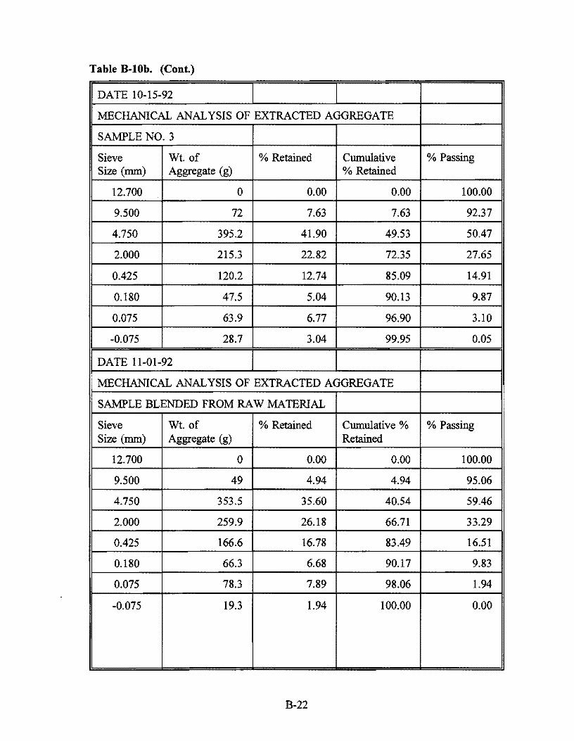
Table B-lOb. (Cont.)
DATE 10-15-92
MECHANICAL ANALYSIS OF EXTRACTED AGGREGATE
SAMPLE NO. 3
Sieve Wt. of % Retained Cumulative % Passing Size (mm) Aggregate (g) % Retained
12.700 0 0.00 0.00 100.00
9.500 72 7.63 7.63 92.37
4.750 395.2 41.90 49.53 50.47
2.000 215.3 22.82 72.35 27.65
0.425 120.2 12.74 85.09 14.91
0.180 47.5 5.04 90.13 9.87
0.075 63.9 6.77 96.90 3.10
-0.075 28.7 3.04 99.95
DATE 11-01-92
I MECHANICAL ANALYSIS OF EXTRACTED AGGREGATE
SAMPLE BLENDED FROM RAW MATERIAL
Sieve Wt. of % Retained Cumulative% % Passing Size (mm) Aggregate (g) Retained
12.700 0 0.00 0.00 100.00
9.500 49 4.94 4.94 95.06
4.750 353.5 35.60 40.54 59.46
2.000 259.9 26.18 66.71 33.29
0.425 166.6 16.78 83.49 16.51
0.180 66.3 6.68 90.17 9.83
0.075 78.3 7.89 98.06 1.94
-0.075 19.3 1.94 100.00 0.00
B-22

Table B-lOb. (Cont.)
i DATE 11-01-92
i MECHANICAL ANALYSIS OF EXTRACTED RUBBER
Sieve Wt. of % Retained Cumulative % % Passing Size (mm) Aggregate (g) Retained
12.700 0 0.00 0.00 100.00
9.500 0 0.00 0.00 100.00
4.750 0 0.00 0.00 100.00
2.000 0.07 0.53 0.53 99.47
0.600 8.862 66.76 67.29 32.71
0.425 1.608 12.11 79.40 20.60
0.180 2.484 18.71 98.12 1.88
PAN 0.25 1.88 100.00 0.00
DATE 11-01-92
MECHANICAL ANALYSIS OF ORIGINAL RUBBER
• Sieve Wt. of % Retained Cumulative% % Passing Size (mm) Aggregate (g) Retained
4.750 0 0.00 0.00 100.00
2.000 0 0.00 0.00 100.00
0.600 0.8 5.33 5.33 94.67
0.425 0.965 6.43 11.77 88.23
0.180 10.652 71.01 82.78 17.22
0.150 1.028 6.85 89.63 10.37
0.075 1.023 6.82 96.45 3.55
-0.075 0.48 3.20 99. 0.35
B-23
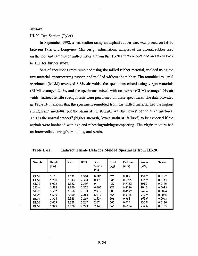
Mixture
IH-20 Test Section (Tyler)
In September 1992, a test section using an asphalt rubber mix was placed on IH-20
between Tyler and Longview. Mix design information, samples of the ground rubber used
on the job, and samples of milled material from the IH-20 site were obtained and taken back
to TTI for further study.
Sets of specimens were remolded using the milled rubber material, molded using the
raw materials incorporating rubber, and molded without the rubber. The remolded material
specimens (MLM) averaged 6.8% air voids; the specimens mixed using virgin materials
(RLM) averaged 2.4%, and the specimens mixed with no rubber (CLM) averaged 0% air
voids. Indirect tensile strength tests were performed on these specimens. The data provided
in Table B-11 shows that the specimens remolded from the milled material had the highest
strength and modulus, but the strain at the strength was the lowest of the three mixtures.
This is the normal tradeoff (higher strength, lower strain at 'failure') to be expected if the
asphalt were hardened with age and reheating/mixing/ compacting. The virgin mixture had
an intermediate strength, modulus, and strain.
Table B-11. Indirect Tensile Data for Molded Specimens from ffi-20.
Sample Height Rice BSG Air Load Deform Stress Strain (cm) Voids (kg) (mm) (kPa)
(%)
CLM 5.151 2.332 2.330 0.086 376 0.889 437.7 0.0182 CLM 5.210 2.332 2.328 0.172 388 0.6985 448.9 0.0143 CLM 5.093 2.332 2.339 0 427 0.7112 505.3 0.0146 MLM 5.532 2.360 2.202 6.695 821 0.4140 894.3 0.0085 MLM 5.552 2.360 2.178 7.712 800 0.4572 867.4 0.0094 MLM 5.519 2.360 2.218 6.017 864 0.3175 942.9 0.0065 RLM 5.398 2.328 2.269 2.534 596 0.381 665.6 0.0078 RLM 5.403 2.328 2.267 2.62 660 0.635 735.8 0.0130 RLM 5.347 2.328 2.278 2.148 668 0.6604 752.6 0.0135
B-24
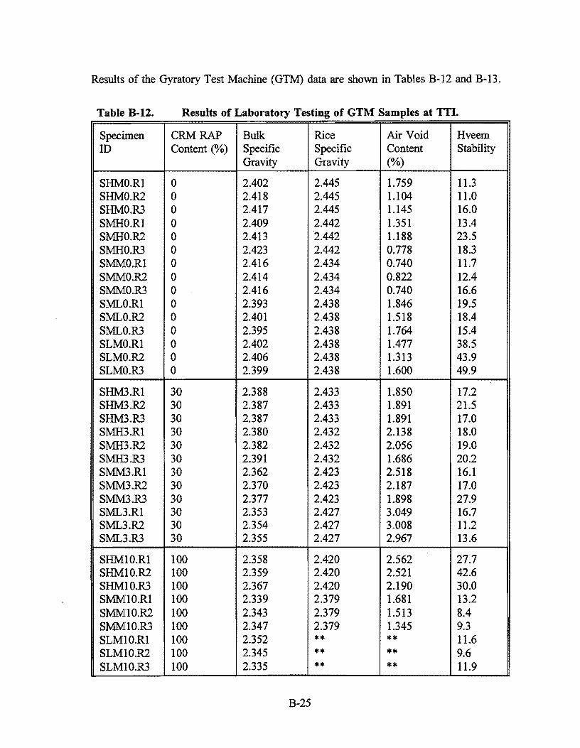
Results of the Gyratory Test Machine (GTM) data are shown in Tables B-12 and B-13.
Table B-12. Results of Laboratory Testing of GTM Samples at TTI.
Specimen CRM RAP Bulk Rice Air Void Hveem ID Content(%) Specific Specific Content Stability
Gravity Gravity (%)
SHMO.Rl 0 2.402 2.445 1.759 11.3 SHMO.R2 0 2.418 2.445 1.104 11.0 SHMO.R3 0 2.417 2.445 1.145 16.0 SMHO.Rl 0 2.409 2.442 1.351 13.4 SMHO.R2 0 2.413 2.442 1.188 23.5 SMHO.R3 0 2.423 2.442 0.778 18.3 SMMO.Rl 0 2.416 2.434 0.740 11.7 SMMO.R2 0 2.414 2.434 0.822 12.4 SMMO.R3 0 2.416 2.434 0.740 16.6 SMLO.Rl 0 2.393 2.438 1.846 19.5 SMLO.R2 0 2.401 2.438 1.518 18.4 SMLO.R3 0 2.395 2.438 1.764 15.4 SLMO.Rl 0 2.402 2.438 1.477 38.5 SLMO.R2 0 2.406 2.438 1.313 43.9 SLMO.R3 0 2.399 2.438 1.600 49.9
SHM3.Rl 30 2.388 2.433 1.850 17.2 SHM3.R2 30 2.387 2.433 1.891 21.5 SHM3.R3 30 2.387 2.433 1.891 17.0 SMH3.Rl 30 2.380 2.432 2.138 18.0 SMH3.R2 30 2.382 2.432 2.056 19.0 SMH3.R3 30 2.391 2.432 1.686 20.2 SMM3.Rl 30 2.362 2.423 2.518 16.1 SMM3.R2 30 2.370 2.423 2.187 17.0 SMM3.R3 30 2.377 2.423 1.898 27.9 SML3.Rl 30 2.353 2.427 3.049 16.7 Sl\1L3.R2 30 2.354 2.427 3.008 11.2 Sl\1L3.R3 30 2.355 2.427 2.967 13.6
SHMlO.Rl 100 2.358 2.420 2.562 27.7 SHM10.R2 100 2.359 2.420 2.521 42.6 SHM10.R3 100 2.367 2.420 2.190 30.0 SMMlO.Rl 100 2.339 2.379 1.681 13.2 SMM10.R2 100 2.343 2.379 1.513 8.4 SMM10.R3 100 2.347 2.379 1.345 9.3 SLMlO.Rl 100 2.352 ** ** 11.6 SLM10.R2 100 2.345 ** ** 9.6 SLM10.R3 100 2.335 ** ** 11.9
B-25

Table B-12. (Cont.)
Specimen CRM RAP Bulk Rice Air Void Hveem ID Content(%) Specific Specific Content Stability
Gravity Gravity (%)
SLM3.Rl 30 2.313 ** ** 19.0 SLM3.R2 30 2.329 ** ** 13.9 SLM3.R3 30 2.321 ** ** 17.5
STM3.Rl 30 ** 2.416 ** ** STM3.R2 30 2.403 2.416 0.538 17.4 STM3.R3 30 2.404 2.416 0.497 22.7
SRM3.Rl 30 2.400 2.401 0.042 ** SRM3.R2 30 2.410 2.401 -0.375 17.5 SRM3.R3 30 2.394 2.401 0.292 12.1
STL3.Rl 30 2.376 2.409 1.370 16.0 STL3.R2 30 2.391 2.409 0.747 16.5 STL3.R3 30 2.385 2.409 0.996 13.0
SRL3.Rl 30 2.406 2.409 0.125 17.8 SRL3.R2 30 2.396 2.409 0.540 14.2 SRL3.R3 30 2.397 2.409 0.498 20.1
PAVE2 0 2.309 2.387 3.268 ** SPEC 1 30 2.275 2.424 6.147 17.3 SPEC2 30 2.270 2.424 6.353 ** SPEC 3 30 2.216 2.424 8.581 ** SPEC4 30 2.222 2.424 8.333 13.8 SPEC 5 30 2.181 2.424 10.025 9.9 SPEC 6 30 2.203 2.424 9.117 ** SPEC lA 30 2.320 2.424 5.000 26.4 SPEC 2A 30 2.320 2.424 4.500 22.3
** Data unavailable
B-26

Table B-13. Final Data for Air Voids at Increments of 10 Gyrations (max. 250 Gyrations).
SLMO SMLO SMMO SMHO SHMO SLM3 SML3 SMM3 SMH3
Gyrations
1 23.586 22.543 17.826 20.327 16.553 20.991 20.764 19.332 16.301 10 16.796 12.667 9.260 10.463 6.842 15.093 11.473 9.510 8.309 20 13.301 9.431 6.425 7.386 4.460 12.124 8.566 6.697 5.721 30 11.302 7.724 4.941 5.789 3.431 10.398 7.027 5.281 4.402 40 9.944 6.614 3.987 4.747 2.968 9.212 6.012 4.479 3.655 50 8.943 5.792 3.370 4.026 2.706 8.351 5.294 3.945 3.183 60 8.165 5.161 2.977 3.523 2.513 7.683 4.767 3.586 2.853 70 7.538 4.683 2.727 3.158 2.356 7.142 4.367 3.313 2.607 80 7.019 4.313 2.543 2.890 2.218 6.694 4.045 3.099 2.416 90 6.587 4.032 2.389 2.679 2.096 6.314 3.789 2.929 2.257
100 6.219 3.805 2.257 2.510 1.985 5.996 3.572 2.790 2.126 110 5.904 3.614 2.139 2.367 1.880 5.727 3.383 2.673 2.009 120 5.630 3.461 2.036 2.242 1.782 5.493 3.226 2.570 1.906 130 5.386 3.325 1.941 2.130 1.683 5.283 3.082 2.473 1.816 140 5.167 3.204 1.851 2.027 1.589 5.102 2.954 2.384 1.730 150 4.966 3.097 1.770 l.934 1.497 4.934 2.842 2.303 1.651 160 4.788 2.998 1.689 1.847 1.408 4.789 2.740 2.217 1.583 170 4.624 2.908 1.612 1.767 1.321 4.610 2.643 2.138 1.517 180 4.475 2.823 1.535 1.691 1.233 4.533 2.553 2.063 1.453 190 4.337 2.740 1.465 1.620 1.148 4.420 2.469 1.990 1.398 200 4.214 2.823 1.399 1.554 1.058 4.316 2.385 1.928 1.339 210 4.100 2.588 1.333 1.488 0.971 4.221 2.303 1.866 1.293 220 3.991 2.518 1.272 1.427 0.881 4.133 2.226 1.809 1.249 230 3.894 2.448 1.210 1.370 0.790 4.051 2.151 1.758 1.200 240 3.796 2.380 1.149 1.313 0.700 3.976 2.078 1.703 1.159 250 3.708 2.317 1.090 1.255 0.610 3.908 2.014 1.641 1.119
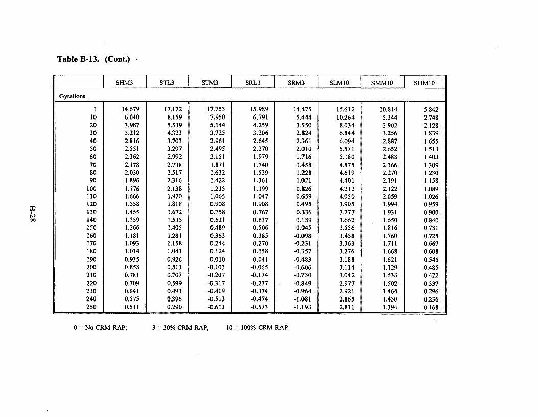
tJ:J I
N 00
Table B-13. (Cont.)
SHM3
Gyrations
1 14.679 10 6.040 20 3.987 30 3.212 40 2.816 50 2.551 60 2.362 70 2.178 80 2.030 90 1.896
100 1.776 110 1.666 120 1.558 130 1.455 140 1.359 150 1.266 160 1.181 170 1.093 180 1.014 190 0.935 200 0.858 210 0.781 220 0.709 230 0.641 240 0.575 250 0.511
0 = No CRM RAP;
STL3 STM3
17.172 17.753 8.159 7.950 5.539 5.144 4.323 3.725 3.703 2.961 3.297 2.495 2.992 2.151 2.738 1.871 2.517 1.632 2.316 1.422 2.138 1.235 1.970 1.065 1.818 0.908 1.672 0.758 1.535 0.621 1.405 0.489 1.281 0.363 1.158 0.244 1.041 0.124 0.926 0.010 0.813 -0.103 0.707 -0.207 0.599 -0.317 0.493 -0.419 0.396 -0.513 0.290 -0.613
3 = 30% CRM RAP;
SRL3 SRM3 SLMlO SMMlO SHMlO
15.989 14.475 15.612 10.814 5.842 6.791 5.444 10.264 5.344 2.748 4.259 3.550 8.034 3.902 2.128 3.206 2.824 6.844 3.256 1.839 2.645 2.361 6.094 2.887 1.655 2.270 2.010 5.571 2.652 1.513 1.979 1.716 5.180 2.488 1.403 1.740 1.458 4.875 2.366 1.309 1.539 1.228 4.619 2.270 1.230 1.361 1.021 4.401 2.191 1.158 1.199 0.826 4.212 2.122 1.089 1.047 0.659 4.050 2.059 1.026 0.908 0.495 3.905 1.994 0.959 0.767 0.336 3.777 1.931 0.900 0.637 0.189 3.662 1.650 0.840 0.506 0.045 3.556 1.816 0.781 0.385 -0.098 3.458 1.760 0.725 0.270 -0.231 3.363 1.711 0.667 0.158 -0.357 3.276 1.668 0.608 0.041 -0.483 3.188 1.621 0.545
-0.065 -0.606 3.114 1.129 0.485 -0.174 -0.730 3.042 1.538 0.422 -0.277 -0.849 2.977 1.502 0.337 -0.374 -0.964 2.921 1.464 0.296 -0.474 -1.081 2.865 1.430 0.236 -0.573 -l.193 2.811 1.394 0.168
10 = 100% CRM RAP

It was found during the course of this study that, if the laboratory creep test is conducted
on short (e.g., 50.8·63.5 mm tall) specimens, end effects are significant (especially if the
specimens are capped). This is illustrated in Figure B·2 where it is shown that a 152.4 mm
tall specimen enters tertiary creep at the same load level applied to a 50.8 mm tall specimen
which does not enter tertiary creep. The shorter specimens are more convenient from a
compaction and coring standpoint. However, the end effects demonstrated here suggest that
the results of the test should be treated as test properties, not material properties, and that
specimen preparation must be consistent and precise. The role of aggregate size versus
height of the specimen has not been studied here, but its effect on creep results should be
studied in the future.
40 1 00% CRM RAP (Tyler) 15.24cm height
35
30
1 0
5
1 0. 16 cm diameter
----------~5.08cm height
O+-----------------------------l
-5+----~----.-----~---~---~------<
0 200
400 600
Time (sec)
800 1200 1000
Figure B-2. Comparison of the Impact of Specimen Height on Creep Response.
B-29
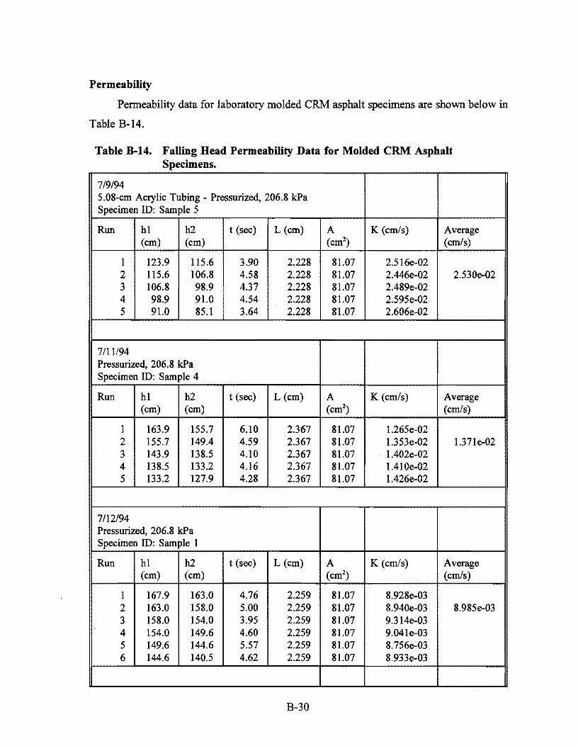
Permeability
Permeability data for laboratory molded CRM asphalt specimens are shown below in
Table B-14.
Table B-14. Falling Head Permeability Data for Molded CRM Asphalt Specimens.
7/9/94 5.08-cm Acrylic Tubing - Pressurized, 206.8 kPa Specimen ID: Sample 5
Run hl h2 t (sec) L (cm) A K (emfs) Average (cm) (cm) (cm2
) (emfs)
I 123.9 115.6 3.90 2.228 81.07 2.516e-02 2 115.6 106.8 4.58 2.228 81.07 2.446e-02 2.530e-02 3 106.8 98.9 4.37 2.228 81.07 2.489e-02 4 98.9 91.0 4.54 2.228 81.07 2.595e-02 5 91.0 85.1 3.64 2.228 81.07 2.606e-02
7111/94 Pressurized, 206.8 kPa Specimen ID: Sample 4
Run hl h2 t (sec) L (cm) A K (emfs) Average (cm) (cm) (em2
) (emfs)
1 163.9 155.7 6.10 2.367 81.07 l.265e-02 2 155.7 149.4 4.59 2.367 81.07 l.353e-02 1.37le-02 3 143.9 138.5 4.10 2.367 81.07 l.402e-02 4 138.5 133.2 4.16 2.367 81.07 l.410e-02 5 133.2 127.9 4.28 2.367 81.07 l.426e-02
7112194 Pressurized, 206.8 kPa Specimen ID: Sample 1
Run hl h2 t (sec) L (cm) A K (emfs) Average (cm) (cm) (cm2
) (emfs)
1 167.9 163.0 4.76 2.259 81.07 8.928e-03 2 163.0 158.0 5.00 2.259 81.07 8.940e-03 8.985e-03 3 158.0 154.0 3.95 2.259 81.07 9.314e-03 4 154.0 149.6 4.60 2.259 81.07 9.041e-03 5 149.6 144.6 5.57 2.259 81.07 8.756e-03 6 144.6 140.5 4.62 2.259 81.07 8.933e-03
B-30

Table B-14. (Cont.)
7/13/94 Pressurized, 206.8 kPa Specimen ID: SML3.Rl
Run hl h2 t (sec) L (cm) A K (cm/s) Average (cm) (cm) (cm2
) (cm/s)
1 156.3 155.9 83 2.377 81.07 4.661e-05 2 155.8 155.4 76 2.377 81.07 5.107e-05 5.537e-05 3 155.3 154.8 85 2.377 81.07 5.728e-05 4 154.7 154.2 89 2.377 81.07 5.491e-05 5 154.0 153.4 88 2.377 81.07 6.697e-05
7/15/94 Pressurized, 206.8 kPa Specimen ID: SRM3 .R3
Run hl h2 t (sec) L (cm) A K (cm/s) Average (cm) (cm) (cm2
) (cm/s)
1 158.8 158.5 336 2.512 81.07 8.979e-06 2 158.5 158.3 302 2.512 81.07 6.670e-06 6.766e-06 3 158.3 158.1 416 2.512 81.07 6.062e-06 4 158.0 157.8 304 2.512 81.07 6.648e-06 5 157.7 157.5 370 2.512 81.07 5.472e-06
7116194 Pressurized, 206.8 kPa Specimen ID: PA VE.2
Run hl h2 t (sec) L (cm) A K (cm/s) Average (cm) (cm) (cm2
) (cm/s)
1 152.4 151.0 5.54 1.309 81.07 1.385e-03 2 151.0 149.6 5.50 1.309 81.07 1.408e-03 1.403e-03 3 149.6 148.1 5.80 1.309 81.07 1.445e-03 4 148.1 146.7 5.64 1.309 81.07 1.400e-03 5 146.7 145.1 6.62 1.309 81.07 1.377e-03
B-31

Table B-14. (Cont.)
7/19/94 Pressurized, 206.8 k:Pa Specimen ID: STL3
Run hl h2 t (sec) L (cm) A K (cm/s) Average (cm) (cm) (cm2
) (cm/s)
1 165.2 164.2 80 2.495 81.07 l.203e-04 2 164.2 163.2 90 2.495 81.07 l.076e-04 l.048e-04 3 163.2 162.4 84 2.495 81.07 9.270e-05 4 162.4 161.6 81 2.495 81.07 9.66le-05 5 161.6 160.7 83 2.495 81.07 l.066e-04
8/1/94 Pressurized, 206.8 k:Pa Specimen ID: SHMIO.R3
Run hl h2 t (sec) L (cm) A K (cm/s) Average (cm) (cm) (cm2
) (cm/s)
1 163.1 158.6 46.9 2.217 81.07 8.400e-04 2 158.6 157.3 15.4 2.217 81.07 7.526e-04 7.124e-04 3 157.3 156.0 15.6 2.217 81.07 7.491e-04 4 156.0 154.7 15.8 2.217 81.07 7.458e-04 5 152.9 152.2 15.6 2.217 81.07 4.142e-04 6 152.2 150.9 15.8 2.217 81.07 7.645e-04 7 150.9 149.7 15.6 2.217 81.07 7.207e-04
8/1/94 Pressurized, 206.8 k:Pa Specimen ID: SLMO.R3
Run hl h2 t (sec) L (cm) A K (cm/s) Average (cm) (cm) (cm2
) (cm/s)
1 165.0 164.0 75 2.155 81.07 l.109e-04 2 164.0 162.9 60 2.155 81.07 1.535e-04 1.406e-04 3 162.9 161.8 60 2.155 81.07 l.546e-04 4 161.8 160.8 60 2.155 81.07 l.414e-04 5 160.8 159.8 60 2.155 81.07 1.423e-04
B-32

Table B-14. (Cont.)
8/2/94 Pressurized, 206.8 kPa Specimen ID: Sample IA
Run hl h2 t (sec) L (cm) A K (cm/s) Average (cm) (cm) (cm2
) (emfs)
1 173.8 169.0 7.40 2.182 81.07 5.245e-03 2 169.0 163.6 8.20 2.182 81.07 5.488e-03 5.417e-03 3 163.6 158.6 7.94 2.182 81.07 5.418e-03 4 158.6 153.5 8.43 2.182 81.07 5.373e-03 5 146.3 141.4 8.49 2.182 81.07 5.56le-03
8/2/94 Pressurized, 206.8 kPa Specimen ID: Sample 2A
Run hi h2 t (sec) L (cm) A K (emfs) Average (cm) (cm) (cm2
) (emfs)
1 169.6 165.4 6.72 2.165 81.07 5.13 le-03 2 165.4 161.0 6.92 2.165 81.07 5.358e-03 5.357e-03 3 159.4 155.4 6.54 2.165 81.07 5.344e-03 4 155.4 151.1 7.20 2.165 81.07 5.359e-03 5 151.1 146.8 7.10 2.165 81.07 5.591e-03
B-33

FIELD STUDIES
NDT (ARAN, FWD, Radar, Pavement Evaluation)
Table B-15 presents data from falling weight deflectometer (FWD) testing. As was
expected at the time this testing was proposed, the FWD does not show any statistically
significant differences between the deflections measmed before and after the inlay at 55
MPa plate loading. The inlay is relatively thin and the measmements were taken within a
few months of each other under similar environmental conditions, so the FWD would not
be expected to show much difference in this scenario. If long term FWD monitoring had
been started several years before the inlay and then continued for several years after the
inlay, the FWD data might have been useful from the standpoint of providing information
on the rate of change of response variables.
Mixture
Table B-16 shows the field densities obtained dming construction of the overlay.
In a demonstration test, the researchers employed two relatively new techniques to
study the job in San Antonio. These two tools were infrared (IR) video and ground
penetrating radar (GPR). The IR video was used to study plant and laydown operations
while the radar was used to study the finished in-place materials.
The CRM RAP mix design resulted in a mix that was similar in natme to a CMHB
in that it appeared to be rich in asphalt and somewhat open or coarse. There was some
concern that the material might be permeable to water. Since this was an inlay application
with no positive drainage installation, a permeable material could result in moistme
accelerated damage with eventual deterioriz.ation of the thick binder films as well as
moistme induced problems in lower layers. The material provided good surface textme for
friction, but this same textme that is beneficial for friction tends to retain water and
increases the time required for a given water particle to reach the pavement edge over that
required to reach the edge on a pavement with the same crown but a smoother textme.
The evaluation of moistme within the pavement layers was evaluated using ground
penetrating radar. Most of the radar study was performed between mile markers 551 and
553 in the westbound lane and just west of the Camp Bullis exit in the eastbound lane. At
B-34

Table B-15. Falling Weight Deflectometer Data Taken Before and After the CRM RAP Inlay.
ime1 Station Load (MPa) Dfl (mm) Df2 (mm) Df3 (mm) Df4 (mm) Df5 (mm) Df6 (mm) Df7 (mm)
A 0.552 55.78745 0.21825 0.08375 0.044 0.031 0.02425 0.01825 0.01375 A 1.123 57.07681 0.28275 0.14075 0.05975 0.02975 0.019 0.01275 0.00975 A l.551 55.10484 0.2465 0.1195 0.05775 0.03425 0.02575 0.0195 0.015 A 3.55 54.28434 0.26625 0.138 0.069 0.03925 0.02725 0.02 0.01575 A 4.552 54.69114 0.22225 0.10375 0.051 0.0325 0.0265 0.019 0.01475 A 7.552 55.0221 0.21025 0.08125 0.0475 0.03375 0.027 0.0205 0.0165
B 0.552 55.87708 0.22125 0.0845 0.044 0.03125 0.02425 O.ot8 0.01375 B 1.072 55.73229 0.2065 0.07275 0.032 0.022 0.02 0.01475 0.01125 B 1.551 55.07037 0.249 0.12 0.0575 0.03475 0.026 0.01925 0.01475 B 3.55 54.24297 0.26975 0.13875 0.069 0.03925 0.02775 0.0205 0.01575 B 4.552 54.84283 0.22625 0.105 0.0515 0.03325 0.026 0.019 0.01475 B 7.552 54.93936 0.2135 0.08075 0.04775 0.03375 0.02675 0.0205 0.01675
1A=After CRM RAP inlay, B=Before inlay.

to I
VJ
°'
Table B-16. Field Densities Obtained During Construction of Original IH-10 Overlay.
Sample Core# Location Nuclear Core (WB Lane) Density Density
(kg/m3) (kg/m3
)
15-92-537 1 471+04 2'R 2143 2098 II 2 421+84 2'R 2166 2087 II 3 369+05 2'R 2134 2038
15-92-542 4 474+64 8'R 2169 2105 II 5 454+44 8'L 2130 1988 " 6 434+59 8'L 2151 2052
15-92-574 7 286+03 2'L 2105 2185 II 8 284+60 8'L 2098 2191 II 9 278+06 4'L 2097 2105
15-92-583 10 248+42 12'L 2042 2203 II 11 238+57 4'L 2001 2145 " 12 224+06 4'L 1972 2126
15-92-584 13 165+02 8'R 2018 2055 II 14 141+62 12'R 1994 2028 II 15 97+67 12'R 1964 2111
% Air Voids
11.4 11.9 14.0 10.6 15.5 12.8 6.8 6.6
10.3 6.4 8.9 9.7 12.4 13.5 10.0
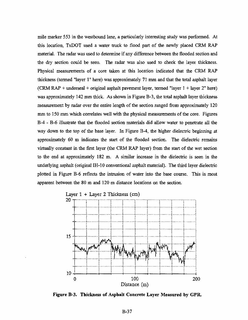
mile marker 553 in the westbound lane, a particularly interesting study was performed. At
this location, TxDOT used a water truck to flood part of the newly placed CRM RAP
material. The radar was used to determine if any difference between the flooded section and
the dry section could be seen. The radar was also used to check the layer thickness.
Physical measurements of a core taken at this location indicated that the CRM RAP
thickness (termed "layer l" here) was approximately 71 mm and that the total asphalt layer
(CRM RAP+ undersea!+ original asphalt pavement layer, termed "layer 1 +layer 2" here)
was approximately 142 mm thick. As shown in Figure B-3, the total asphalt layer thickness
measurement by radar over the entire length of the section ranged from approximately 120
mm to 150 mm which correlates well with the physical measurements of the core. Figures
B-4 - B-6 illustrate that the flooded section materials did allow water to penetrate all the
way down to the top of the base layer. In Figure B-4, the higher dielectric beginning at
approximately 60 m indicates the start of the flooded section. The dielectric remains
virtually constant in the first layer (the CRM RAP layer) from the start of the wet section
to the end at approximately 182 m. A similar increase in the dielectric is seen in the
underlying asphalt (original IH-10 conventional asphalt material). The third layer dielectric
plotted in Figure B-6 reflects the intrusion of water into the base course. This is most
apparent between the 80 m and 120 m distance locations on the section.
Layer 1 + Layer 2 Thickness (cm) 20
t·:·· :::1 :··:··· :•1: :·••::• :1:::. • :•::I:::::::: f ::: : : : ::: :::::::: :: 1::: ::: ::: t:: •: :•:: 1:: :: •: :: :1
········l·········l·········1········+······+········l·········I········+ .. ····+········, 15 ·: : :: : :1 :::::::: r :: : :: r:::: +::::: :: 1 :: ::::: ! · : .. :·. :: F· . f ·: •-: • :· f .. : ·: • :: I
10 l i l l i i I l I I 0 100 200
Distance (m)
Figure B-3. Thickness of Asphalt Concrete Layer Measured by GPR.

Dielectric Property Index, Layer 1
10
: :.: ·1: :::::r::::.r:::::F::: '. ··:::·· ,·::::::: : ::·:.·r:::] :.: .. : ........ ~-·~··················· ·········-:····•+••··::--··-······1·~····
4 -+-~-l-~-·1--~-1--~~\~--+l~--+l~___.~~!--~J-------l 0 100
Distance (m)
Figure B-4. Dielectric Property for Layer 1 (CRM RAP).
0 100 Distance (m)
200
200
Figure B-5. Dielectric Property for Layer 2 (Original Conventional Asphalt).
B-38

. . . l
::::l :: ········-r·········1 ........ r···· .. ·: i
200
Figure B-6. Dielectric Property for Layer 3 (Base Course).
It is apparent that this permeability and air void content are not low enough to keep
water from entering the pavement system. It remains to be seen how detrimental such water
intrusion will be to the life of the pavement. However, it is clear that a positive drainage
system would have improved its chances for a long life.
The infrared video provided interesting data on equipment and material temperature
and operating characteristics. It is obvious from the videotape that the hand.held IR
thermometers and mercury thermometers are vastly inferior to IR video for temperature
measurement of the mat. Problems with the laydown machine and the freshly laid material
that were invisible to the naked eye were easily identified with IR video. Limited laboratory
investigation using surface temperature measurements on CRM RAP specimens with varying
percentages of RAP content had indicated that the specimens with higher rubber contents
cooled faster than those with lower rubber contents (50% and 100% CRM RAP mixtures
were compared). Because the haul from the plant to the construction site was so long, there
was some concern that the mix would be too cool at laydown. IR video was used to track
a load of material from the plant to laydown and compaction. Figures B-7 - B-9 illustrate
the temperature change of this load of material. Even for this haul length, heat retention
seemed to be adequate in the environmental conditions encountered during the job.
B-39

Windrow
140
~ 120 x Q) x 5 0 100 a; Cl... E ~ 80
60
X Laydown a: Compoctton
x
xx x
x
40-+-~~....-~--,-~~-...-~~.....-~~.,--~--,~~.........-~~....,-~~....-~-x'--'!
140
~ 120 Q)
5 0 100 a; ~ ~ 80
60
0 50 100 150 200 250 300 350 400 450 500 Time (min)
Figure B-7. IR Temperature History at Test Point 1.
Windrow
X L.aydown &: Compaction
x
x x
x x
x
40-r-~~,...-~--,~~-,...~~-r-~~-.-~--,,.--~--..~~-,-~~...,.-~---:
0 50 1 00 150 200 250 300 350 400 450 500 Time (min)
Figure B-8. IR Temperature History at Test Point 2.
B-40

8: 120 ., 5 ~ 100
~ E ,'! 80
60
isr ...... L-)1(
)(
tEll'Sldt~Roilr'
- i<-sio. )(
40+---..-~-..--~--...---,--.--..---.-----1
0 50 100 150 200 250 300 350 400 450 500 Time (min)
Figure B-9. IR Temperature History at Test Point 3.
Therefore, although long hauls are not recommended, they are feasible when properly
undertaken.
The effect of plant variability on several different mixture parameters can be seen in
Figures B-10 through B-18.
9.5
,..... 9 ~
~ 8.5
~ = 8 l
Asphalt Con1enl
.: 7.5
7
6.5 _.__,___,.__,-..--..--....--.-....-~-...--,.---.,...--..--,-,......J 7-15 17 23 25 28 31 6 7
Days Plant Run
Figure B-10. Asphalt Content for Original CRM RAP Project.
B-41

13 • No air voids for this dote
1 2 .. -~ 11 I '-'
(/)
"O ·o > ....
<{ ..... c C>
E C> > 0 a..
10
I 9
J 8
7 ~
• * • * 6
7-15 17 23 25 28 31 6
July Doys Plont Run
August
Figure B-11. Air Voids for Original CRM Project.
Cl)
>
28
ill 26
E E
N 24 C> c ·;;;
"' ct' 22 ~
20
7
18-'---r-----r~--.-~-,-~-..---.~--.-~-,-~..,----,~.....,-~-,-~..,.----,r---r-'
7-15 17 23 25 28 31 6 7 Days Plont Run
Figure B-12. Percent Passing 2 mm Sieve for Original CRM Project.
B-42

6.5
E 6 E
I,()
~ 5.5 0 Ol
.E 5 "' "' 0
a.. ~ 4.5
4
assing 0.075mm
\ 3.5-'--~~~~~~~~~~~~~~~~~~~~....--~~~~
7-15 17 23 25 28 31 6 7 Days Plant Run
Figure B-13. Percent Passing 0.075 mm Sieve for Original CRM Project.
100
99.5
99
98.5
..?::- 98 ·v; c: ~ 97.5 ..0 0 97 .....I
96.5
96
95.5
95 7-15 17 23 25 28 31 6 7
Days Plant Run
Figure B-14. Laboratory Density for Original CRM Project.
B-43

7.5
7
~6.5 .__...
<: 6 Cll
<: 8 5.5 ..... c 5 ..c a_
"' <( 4.5
4
3.5
3~~~~~~~~~~~~~~~~~~~~~~~~~~
10-04 05 06 08 Days Plant Run
Figure B-15. Asphalt Content for CRM RAP Project (October 1993).
10
9 -
8-..-.. ~ 7-.__...
"' "'C 6 -"Ci
>
/ '- 5-<{
c 4-Cl>
E Cl> > 3 -c
a..
2 -
1 -
0 10-04 05 06 08
October Days Plant Run
Figure B-16. Air Voids for CRM RAP Project (October 1993).
B-44

30
28
26 Q)
~ 24 i.ii E 22 Pessin mm E
N 20 Cl c:
18 -·v; V> 0
0.. 16 ~
14
12
10 10-04 05 06 08
October Days Plant Run
Figure B-17. Percent Passing 2 mm Sieve for CRM RAP Project (October 1993).
o~..,..---,~--..-~-.-~.,.----.~-.-~-.-~..----..~-,-~-.-~...----..~--..-~
10-04 05 06 08 Days Plant Run
Figure B-18. Percent Passing 0.075 mm Sieve for CRM RAP Project (October 1993).
B-45


APPENDIX C - ASPHALT RUBBER RECYCLING GUIDELINES
CONSTRUCTION ALTERNATIVES
Epps et al. (1980) identify twenty-four alternatives for recycling asphalt concrete
pavements. Recycling methods are generally used to improve surface distress, structural
inadequacy, ride quality, and skid resistance of a pavement. The differences are primarily
in the depth of the recycle, the presence or absence of heat, and the presence or absence of
new binder in the recycle. These alternatives are divided into three broad categories:
surface, in-place, and central plant recycling.
Surface Recycling
This technique involves reworking the surface of a pavement to a depth of less than
25 mm (I in.). This procedure is presently the most popular form of recycling to address
a wide variety of pavement distress, including rutting, raveling, flushing, and corrugation.
However, it has only a very limited effectiveness in repairing severely rutted roads or in
significantly increasing the load-carrying capacity of the roadway.
The equipment used in recycling techniques requiring heat are heater planers, heater
scarifiers, and hot millers. Cold recycling uses cold planers and cold millers. A guide to
equipment alternatives is provided below.
Heater Planer
The heater planer maintains longitudinal grade and transverse cross slope, and is ideal
for heating and planing a pavement prior to overlay. Also, to correct poor skid resistance
in flushing or bleeding asphalt rubber mixes, the heater is used to heat the pavement while
a seal-coat aggregate is spread and imbedded into the distressed pavement with a steel-wheel
roller.
C-1

Heater Scarifiers
Heater scarifiers remove pavement surface regularities. When a new wearing course
is desired after scarification, the heater scarifier may improve the bond between old
pavement and new asphalt rubber overlay.
Hot and Cold Millers
Milling operations improve the surface texture of the roadway. This improved surface
texture increases skid resistance as well as the shear strength between the old surface and
a new overlay. The millings can be treated either in-place or at a central plant, and can be
used for unstabilized base courses or stabilized base and surface courses. With asphalt rubber
mixes, the use of heat often results in milled rubber particles sticking to equipment, so cold
milling provides a less problematic alternative.
Cold Planers
Cold planing is commonly used to remove corrugations and improperly constructed
chip seals. While it does not provide a surface appearance as smooth as heater planing, heat
free planing does not result in high emission levels of air pollutants, making it the most
environmentally safe alternative.
In-Place Surface Recycling
In-place surface recycling has resulted from the development of pulverizing equipment
and processing techniques, and has a major advantage of improving the load-carrying
capability of the pavement without changes in the geometry of the roadway. Two basic
approaches can be used, depending on the thickness of the asphalt concrete surface. If the
surface is about 125 mm (5 in.) thick or less, pulverization equipment can be used without
preliminary ripping and breaking. For a thicker surface, scarifiers, dozers, or compactors
may be used for the initial breakup, followed by a pulverization process.
The disadvantages of in-place surface recycling are that quality control is not as good
as with central plant operations, and traffic disruption may be relatively high.
C-2

Central-Plant Recycling
The pavement is ripped and broken to a size to be received by the primary crusher
prior to loading onto the haul units. The pavement can be reduced in size in-place and then
hauled to the central plant, or can be removed from the site and then sized using other
equipment. When reused at the plant, the recycled hot mix process involves the use of
additional heat and recycling agents.
Central-Plant sizing can be performed with conventional, fixed, and portable crushing
and screening equipment. It maintains good quality control, although at a high cost.
Selection of central plant recycling alternatives depends on the availability of plant
equipment, the need for structural improvement, and the distance of haul to new aggregate
and existing plants. With CRM asphalt mixes, the plant should have the necessary
modifications to allow for sticky rubber at high mixing temperatures. The following
guidelines are owed in large part to recommendations taken from the FHW A Crumb Rubber
Modifier workshop of 1993.
STORAGE AND HANDLING OF CRM
Crumb rubber is commonly packaged in polyethylene bags of approximately 27 kg
(60 lbs), or larger bulk of approximately one ton in capacity. Both forms of rubber
packaging are pelletized and require tied-down plastic sheeting for additional moisture
protection during storage. Crumb rubber pellets are handled with forklifts and standard
conveyor belts are used for polyethylene bags. The rubber is generally fed into the weigh
hopper or pug mill of a batch plant or the RAP feed system on a drum plant. Where graded
CRM is used, dispersion of the rubber throughout the hot mix must be ensured.
C-3

HOT MIX EQUIPMENT AND PRODUCTION
A conventional hot mix asphalt mixing facility can be modified with automatic
controls that coordinate proportioning, timing, and discharge of the mixture. The facility
shall be capable of uniformly feeding and measuring the amount of crumb rubber placed
into the mixing chamber, with the capability to heat binder supply lines.
When a drum plant is used, the metering equipment is hooked up by installing a two
or three-way valve in the feed line on the output side of the asphalt pump. The metering
equipment is then plumbed to the valve to feed the asphalt rubber binder accurately to the
hot mix plant. Special pumps are used to prevent damage to conventional pumps.
When a batch plant is used, the valve is installed directly onto the supply line leading
to the weigh bucket and the metering equipment is plumbed as described above.
Asphalt rubber shall not be transported on rubber belts. Cold CRM RAP may be
transported on rubber belts.
The crumb rubber shall not be added to the aggregate cold feed system, but will be
added beyond the drying and heating section of the mixing chamber. CRM RAP must be
crushed to a size that can be adequately heated in the drum. This is usually done at the
beginning of the feed system to the RAP collar.
PAVING EQUIPMENT
Distributor
The distributor shall be capable of uniformly applying the asphalt rubber binder at the
specified temperature and application rate, while providing continuous circulation of the
binder in the tank for homogeneity until it is metered into the hot mix facility mixing
chamber.
C-4

Aggregate Spreader
The aggregate spreader shall be self-propelled and of sufficient capacity to apply the
aggregate within the specified time.
Hauling Equipment and Rollers
The hauling equipment and compaction rollers may be thinly coated with a light
application of non-petroleum based wetting agent such as soapy water or silicone emulsion
to reduce sticking of the mixture to the equipment. Oiling the surfaces with kerosene or
diesel fuel will not be permitted. The rollers shall be steel-wheeled and capable of reversing
without backlash. Each tire shall be inflated to a minimum of 700 kPa (100 psi) and carry
a minimum of 1,360 kg (3,000 lb). Pneumatic-tired rollers may only be used with surface
treatments containing asphalt rubber binder, and with mixtures having up to 30% CRM RAP
content. Beyond 30% CRM RAP, the use of rubber-tired rollers should be considered
experimental until sufficient data indicates otherwise.
OTHER CONSTRUCTION GUIDELINES
Weather
For a compacted thickness less~ 38.1 mm (1.5 in.), the application of an asphalt
rubber surface treatment shall only be permitted at a minimum surface and ambient air
temperature of 15°C (60°F). For a compacted thickness 3.81 cm (1.5 in.) and greater, the
minimum temperature requirements shall be l0°C (50°F).
Delays
When a delay in surface treatment application occurs, the asphalt rubber binder shall
be allowed to cool. Just prior to use, the asphalt rubber shall be reheated to the specified
C-5
mixing temperature, thoroughly mixed, and the viscosity checked. The asphalt rubber binder
shall be rejected if the viscosity fails specifications.
Application of the Binder
The binder viscosity may be adjusted to improve spray application by adding a
kerosene diluent. This should occur in the distributor immediately prior to the spray
application. When a diluent is used, the binder temperature for spraying shall not exceed
1so·c (300°F).
LAYDOWN AND COMPACTION
Temperature
The following temperature ranges are common for asphalt rubber hot-mix applications:
(a) Hot plant mixing temperature 138 to 154°C (280 to 310°F)
(b) Laydown temperature 132 to 149°C (270 to 300°F)
(c) Compaction temperature above 115°C (240°F)
At lower CRM RAP contents (e.g., 30%), temperatures are similar to conventional mixtures
without rubber.
Breakdown Rolling
Use two to four passes in the vibratory mode (full width of mat) with a double drum
steel wheel roller, high frequency , low amplitude. Pneumatic rollers should NOT be used
on new (100%) CRM pavements. Steel drums should be equipped with pads and a watering
system.
C-6
RELATED PUBLICATIONS
ASTM C29, Test Method for Unit Weight and Voids in Aggregate.
ASTM C127, Test Method for Specific Gravity and Absorption of Coarse Aggregate.
ASTM Cl28, Test Method for Specific Gravity and Absorption of Fine Aggregate.
ASTM D5, Penetration of Bituminous Materials.
ASTM D1856, Recovery of Asphalt from Solution by Abson Method.
ASTM D4887, Practice for Preparation of Viscosity Blends for Hot Recycled Bituminous Materials.
ASTM D4791, Test Method for Flat or Elongated Particles in Coarse Aggregate.
Chehovits, J.G., "Binder Design Procedures," Crumb Rubber Modifier Workshop Notes, Design Procedures and Construction Practices, FHWA, Session 9.
Cooper, K.E., S.F. Brown, and G.R. Pooley, "The Design of Aggregate Gradings for Asphalt Basecourses," Asphalt Paving Technology, AAPT, Vol. 54, pp. 324-345.
Epps, J.A., "Uses of Recycled Rubber Tires in Highways," NCHRP Synthesis of Highway Practice 198, 1994.
Lovering, W. R. and J. Matthews, "Design and Control of Asphalt Mixes," Institute of Transportation Studies, Course Notes, University of California, Berkeley, May 1978.
Roberts, F.L., P.S. Kandhal, E.R. Brown, D-Y Lee, and T.W. Kennedy, Hot Mix Asphalt Materials, Mixture Design, and Construction, NAPA, 1991.
AASHTO TP7, Standard Method for Determining the Permanent Deformation and Fatigue Cracking Characteristics of Hot Mix Asphalt (HMA) Using the Simple Shear Test (SST) Device.
Tex-200-F, Sieve Analysis of Fine and Coarse Aggregate.
Tex-201-F, Bulk Specific Gravity and Water Absorption of Aggregate.
Tex-206-F, Method of Compacting Test Specimens of Bituminous Mixtures.
Tex-210-F, Determination of Asphalt Content of Bituminous Mixtures by Extraction.
C-7

Tex-211-F, Recovery of Asphalt from Bituminous Mixtures by the Abson Process.
Tex-224-F, Determination of Flakiness Index.
Tex-231-F, Static Creep Test.
Tex-232-F, Mixture Design Procedure for Crumb Rubber Modified Asphaltic Concrete.
Tex-234-F, Mixture Design Procedure for Coarse Matrix High Binder Asphaltic Concrete.
Tex-404-A, Determination for Unit Weight of Aggregate.
Tex-405-A, Determination for Percent Solids and Voids in Aggregate for Concrete.
Tex-410-A, Abrasion of Coarse Aggregate by Use of the Los Angeles Machine.
Tex-502-C, Test for Penetration of Bituminous Materials.
Texas Construction Specification Item 300, Asphalts, Oils and Emulsions.
Texas Construction Specification Item 340, Hot Mix Asphaltic Concrete Pavement.
Tunnicliff, D.G., "A Review of Mineral Filler," Proceedings of The Association of Asphalt Paving Technologists, Volume 31, 1962, pp. 118-150.
SCOPE
The goal of this procedure is to provide guidance for the design of bituminous
mixtures containing crumb rubber reclaimed asphalt pavement (RAP). It should be used in
conjunction with applicable Texas Construction Specifications such as Items 300 and 340.
In most cases, the RAP is available because the pavement is performing inadequately. This
inadequate performance is usually caused either by improper mixture design or improper
construction techniques. Both sources of difficulty are addressed in the procedure.
The first objective is to design a mixture which will ensure that the load is carried by
the stone skeleton. For aggregate blending purposes, meeting this objective implies that any
rubber particle greater in size than the asphalt film thickness should be considered as part
of the aggregate. Note that the previous statement does not necessarily mean that the rubber
influences the behavior of the mix in the same way as the aggregate; rather the intent is to
C-8

provide sufficient room within the aggregate skeleton for the rubber to act primarily as a
binder modifier. In order to facilitate portability of the procedure between the laboratory
and the plant, the procedure emphasizes RAP and virgin material stockpile characteristics
at the plant. Therefore, the second objective is to ensure that the aggregate in the largest
stockpile to be used in the mixture actually participates in carrying the load. This objective
can be generalized to all stockpiles to be used in the mix if more than one stockpile is used.
The third objective is to provide for adequate binder film thickness for the intended use of
the material without allowing draindown. The design procedure is intended for use with
standard hot mix applications as given in the example, but can be easily modified for use
in special applications such as open-graded drainage or friction courses by choosing the
correct stockpile characteristics and employing crumb rubber to reduce draindown and
possibly oxidation problems. Therefore, in standard mix applications using this procedure,
it is expected that no rubber will be added with the new material; the only rubber in the mix
will be that already present in the RAP. For open-graded designs, however, additional
crumb rubber may be necessary. In the latter case, it is anticipated that the wet process will
be used to incorporate the rubber.
The final objective is to provide a binder that has the desired performance
characteristics. This can be done through asphalt binder blending tests. Successfully
reaching this objective should not affect the aggregate blending calculations. However, there
is one case in which it will affect the aggregate blending calculations. That case is the one
in which the addition of virgin binder and/or rejuvenator required to reach the desired
asphalt binder performance characteristics overfills the available voids. In the event this
problem arises, the recommended actions are, in order of preference, (1) decrease the RAP
content, (2) decrease the viscosity of the virgin binder/rejuvenator, and/or (3) use a virgin
stockpile that has a gradation favoring an increased asphalt content but still meets the stone
on-stone contact requirements.
The philosophy adopted in this procedure implies that there is no specified minimum
or maximum RAP content in the final mix. This means that, for example, an 80% RAP
content may result from the design. In practical terms, such a high RAP content requires
that conventional plant production rates must be reduced if the RAP is either wet or not
C-9

sufficiently crushed. Relatively new recycling equipment1 has been or is being developed
to address the challenges presented by higher RAP content mixtures.
EVALUATE RAP
1. Prepare specimens of the RAP (100% RAP, no modification to the reclaimed
material). Evaluate these specimens with the specifications and design criteria of T ex-231-F
and Tex-232-F. If stripping is suspected, evaluate the RAP using Tex-530-C and Tex-531-C
as well.2 If the RAP passes these criteria, it is assumed that the material is acceptable to
TxDOT and that the reason the material failed was because of improper construction
techniques. In this case, it is unnecessary to modify the RAP prior to reuse; a 100% RAP
recycle is feasible (assuming any moisture problems can be overcome in the plant, and
assuming that any underlying pavement structural problems have been corrected), and no
further testing is required under this procedure. However, if the RAP does not meet current
TxDOT criteria and specifications, the remainder of this procedure must be accomplished.
2. Obtain an approximate asphalt content (Tex-210-F), crumb rubber size, and sieve
analysis of the RAP (Tex-200-F).3 When performing the extraction of Tex-210-F, pay
particular attention to the notes on crumb rubber. It may be necessary to add steps to
recover the. rubber as well. This is usually done by floating the rubber using a sodium
1e.g. RAPMaster, Pyrotech, Cyclean.
2Recent advances in more fundamental tests for bond characteristics in the presence of fluids such as water will probably result in an improved method that will replace these test methods in the near future.
31t has been found (e.g., Epps 1994 p. 30, as well as in study 1333) that an accurate measure of asphalt and rubber content and properties is not possible with most current solvent extraction tests. This is thought to be a result of the interaction of the solvent with the rubber and asphalt and is related to the swelling of the rubber as well as small quantities of rubber going into solution in the asphalt over time. Therefore, asphalt and rubber contents and properties obtained through solvent extraction methods should be considered to be approximate. Performance based tests and specifications refine this approximation. It has also been found in California that nuclear gauges should not be used for determination of total binder content (Epps 1994).
C-10

bromide solution. However, citrus terpene has been used for floating with some success.
After extraction, the asphalt should be recovered (Tex-211-F). Reblend the recovered
asphalt and floated rubber particles. At this point, the normal procedure would be to
measure the viscosity of the recovered asphalt rubber blend (Tex-528-C) for use in viscosity
blending (ASTM 04887).4 However, this viscosity measurement may not be possible for
some blends, and it has already been shown that current extraction procedures alter the
characteristics of the asphalt and rubber. Therefore, simply save the recovered and
reblended CRM asphalt binder for later use in blending tests. Enough binder should be
extracted, recovered, and reblended with the recovered rubber to perform 4 penetrations at
25°C (l 10°F), and 1 additional penetration at 35°C (160°F). Finally, one additional
extraction should be performed to obtain a sample of aggregate and rubber. Recovery of
this asphalt is not necessary, but the rubber must be recovered as part of the aggregate for
use in the vibration tests later in the procedure.
3. Perform a sieve analysis on the aggregate from the extraction. Using the clean
aggregate (no rubber) from the extraction, determine the RAP size at 50% passing (i.e., D50
size) by linear interpolation between the two sieve sizes on either side of the 50% passing
mark.
4. Measure the dry bulk specific gravity and absorption (Tex-201-F, ASTM Cl27,
Cl28) of the extracted aggregate-rubber blend.
5. For purposes of this procedure, the crumb rubber is assumed to have a specific
gravity of 1.15, and a surface area of 150 cm2/g (60 in2/g) (see gas absorption results given
by Chehovits 1993). However, if 100% of the crumb rubber will not pass through a 0.635
cm (.25 in) sieve, a sieve analysis should be conducted on the rubber and the surface area
should be either calculated using the surface area factor methodology or measured.
6. Measure the penetration of the recovered asphalt rubber blend at 25°C (l 10°F).
4lt is expected that in the near future, performance grading type analyses using rheometers will become preferred methods of determining blending needs. However, some rheometers do not currently have the capacity to test crumb rubber modified asphalt binders, and procedures using rheometers that do have that capacity at present are still in the development stage (e.g., plate spacings on torsional shear rheometers is still somewhat subjective).
C-11

EVALUATE VIRGIN MATERIAL
1. Using the sieve analyses from the plant stockpiles that will be used on the job,
select the stockpile(s) of virgin material having a D50 size that is greater than the D50 size
of the RAP. For open graded applications, it may be necessary to select a stockpile with
even larger materials instead.
2. Measure the dry bulk specific gravities and absorption (Tex-201-F, ASTM C127,
C128) of each stockpile of material that may be a candidate for use in the final bituminous
mixture.
3. Measure the penetration of the available potential rejuvenating agents and/or virgin
asphalts at 25°C ( 110°F). 5 Of the available potential rejuvenating agents and virgin
asphalts, it is thought that those having the higher aromatic-to-saturate ratios and lower
asphaltene contents from a Corbett analysis of the asphalt fractions will provide lower
hardening susceptibility.
DESIGN NEW BLEND
1. Perform the following modified tests using the LA Abrasion (or ball mill)
equipment if available.
(a) Wash the largest stockpile material on a 9.5 mm (3/8 in) sieve and dry the
+9.5mm (3/8 in) material. Run the LA abrasion using the steel balls. Wash the abraded
material on the 9.5 mm (3/8 in) sieve. Compute the modified LA abrasion. This portion
of the procedure is a surrogate test for a fracture mechanics type test on the large aggregate.
It is intended to quantify the friability of the material and give some qualitative indication
5Potential rejuvenators include a wide range of materials such as low viscosity asphalts and asphalts which have viscosities that have been reduced by the addition of proprietary solutions. In this procedure, the term rejuvenating agents refers to additives such as these proprietary solutions or even solutions containing crumb rubber. Asphalts, regardless of grade, are considered to be virgin asphalt cements only if they contain no additives or modifiers.
C-12

of any tendency toward breakdown of the larger particles under compaction equipment or
traffic.
(b) Combine the stockpiles so as to give a gradation curve that falls between the 0.5
and 0.7 Fuller power curve gradation (the power curve formula is given in Equation C-3
later in the procedure). Split the sample in half and perform a sieve analysis on one of
these two samples. Take the other half and run 5 minutes in the LA machine without the
steel balls (the wet ball mill Tex-116-E without the water and without the balls is an
acceptable substitute for the LA machine). Sieve the abraded material.6 This portion of
the procedure is intended to simulate the action of the hot mix plant. The change in
gradation from the original to the abraded material will affect asphalt content.
2. For each stockpile of material and for the aggregate-rubber blend extracted from
the RAP, perform the following measurements on dry aggregate samples.
(a) Vibrate the dry aggregate in a suitably sized container (e.g., a unit weight bucket)
that has a weighted lid which will follow the material as it rearranges its particle orientation
to a more dense state. If a vibratory table is not available, use a tamping or jigging
procedure as in ASTM C29 (Tex-404-A7), or a high capacity sieve shaker may suffice. At
the end of the densification process, measure and record the height of the lid at three points
120° apart. Remove the lid and loosen the aggregate. Repeat the vibration and
measurements two more times. After the third vibration test, do not loosen the material,
simply remove the lid and, if a water measurement is desired (optional for this procedure),
fill the container with water up to the average level of the irregular aggregate surface.
Weigh the container, aggregate, and water. Compute the weight of the water by subtraction
using the data from step (a) above. Compute the volume of this water. Compute the
volume taken up by the aggregate plus air and the volume of the air in the densified state
using the previously measured dry bulk specific gravity of the aggregate and the average of
6Recovering the material from the LA machine implies that the door on the drum is essentially air tight so that fines are not lost during the test. This often requires modification to the door (e.g., weatherstrip application).
7Note that this procedure differs from Tex-404-A in that a full measure is not required because measurements are taken of the compacted height of the specimen.
C-13

the 9 height measurements. Record both the volume of water (if measured) and the volume
of air (from height measurements).
The intent is to fill as much of the available volume as possible with the next smaller
aggregate size stockpile and continue that process down through the stockpiles. However,
before this next smaller stockpile can be used, it is necessary to determine if the largest
particle size in this stockpile will separate the particles of the large stockpile and tend to
decrease the effectiveness of this stockpile in the stone skeleton. Based on computations of
available void size using several geometric configurations (e.g., spherical particles in a
hexagonal close packed configuration, elongated particles in a triangular configuration), the
following guidelines for acceptability of the aggregate in the next smaller size stockpile,
DMAXi• were formulated. For uncrushed, rounded gravel type aggregates, the size at 50%
passing (i.e., D50 size) of the second stockpile must be equal to, or smaller than, 0.15 times
the D50 size of the largest size in the first (larger) stockpile. For cubical (ratio of all lengths
are 1: 1) aggregate with at least one crushed face, the D50 size of the second stockpile must
be equal to, or smaller than, 0.29 times the D50 size in the first (larger) stockpile. For
elongated particles (ASTM D4791 uses 2:1 as the length to width ratio), the D50 size of the
second stockpile must be equal to, or smaller than, 0.40 times the D50 size in the first
(larger) stockpile. For this test procedure, it is adequate to determine the prevailing shape
in the largest stockpile subjectively, and to use the factor corresponding to that shape for
calculations involving all other stockpiles (in the future, a relationship between this factor
and fractal dimensions of the aggregate from digitized video imaging should be developed).
The 0.40 factor is used in the example. Note that D50 and DMAxi are rounded to two decimal
places in cm units before the decision to accept or reject the stockpile is made.
Each stockpile that meets the size restrictions is then used in the proportioning
process. The proportioning can be done on a volumetric or on a weight basis. Each size
fraction is adjusted for differences between the laboratory and the plant during the final
blend gradation computations. In the research program, this adjustment was made by
computing the ratio of the percent passing a particular size after LA abrasion to that passing
prior to LA abrasion. If measurements are not available to compute this ratio, the following
equation may be used to approximate the ratio. Note that this equation was developed for
C-14

a limestone and bank run sand material and may not be representative for materials that do
not have comparable LA abrasion values (on the order of 21 % was measured for the
limestone). The equation is valid for S:s;S.08 cm (use a ratio of 1.0 for larger particles
unless measurements indicate a larger value):
R1P - 1.242 (5.08-Smax +S)-0·133 (C-1)
where s is the square sieve opening size in cm, smax is the size of the largest sieve that has
less than 100% passing (all sieves having 100% passing are arbitrarily assigned a value of
R1P=l.O), and R1P is the lab-to-plant adjustment ratio.
3. After the acceptable stockpile(s) have been used to fill the open volume, the
remaining free volume is that available for binder assuming nonabsorptive aggregate and
zero air voids. The initial choice of binder content is based on surface area factors using
Equation C-2. Later in the design process, these surface area factors are applied to the
percent retained as modified by the LA Abrasion tests (ratio of percent passing each size
after abrasion to percent passing before abrasion) to obtain the surface area of the size
fraction under study. Surface area factors have been computed on the basis of a cube with
the same dimensions as the square sieve opening, a sphere having a diameter equal to the
opening size, and a prolate spheroid (football shape) with the long axis along (but shorter
than) the diagonal measurement for the square sieve opening size. The surface area factor
formula for the cube and sphere is the same and can be obtained by the very simple formula
6 SAF- -Sy
(C-2)
where SAF is the surface area factor in cm2/g, and y is the unit weight of the aggregate in
g/cm3• A tabular summary of the surface area factors and lab to plant adjustment ratios
based on the equations presented above is given in Table C-1.
The asphalt content is determined by specifying a desired film thickness. The desired
film thickness is assumed to be a function of the gradation (and rubber content). Therefore,
one must compute the exponent of the gradation resulting from the stockpile blending
C-15
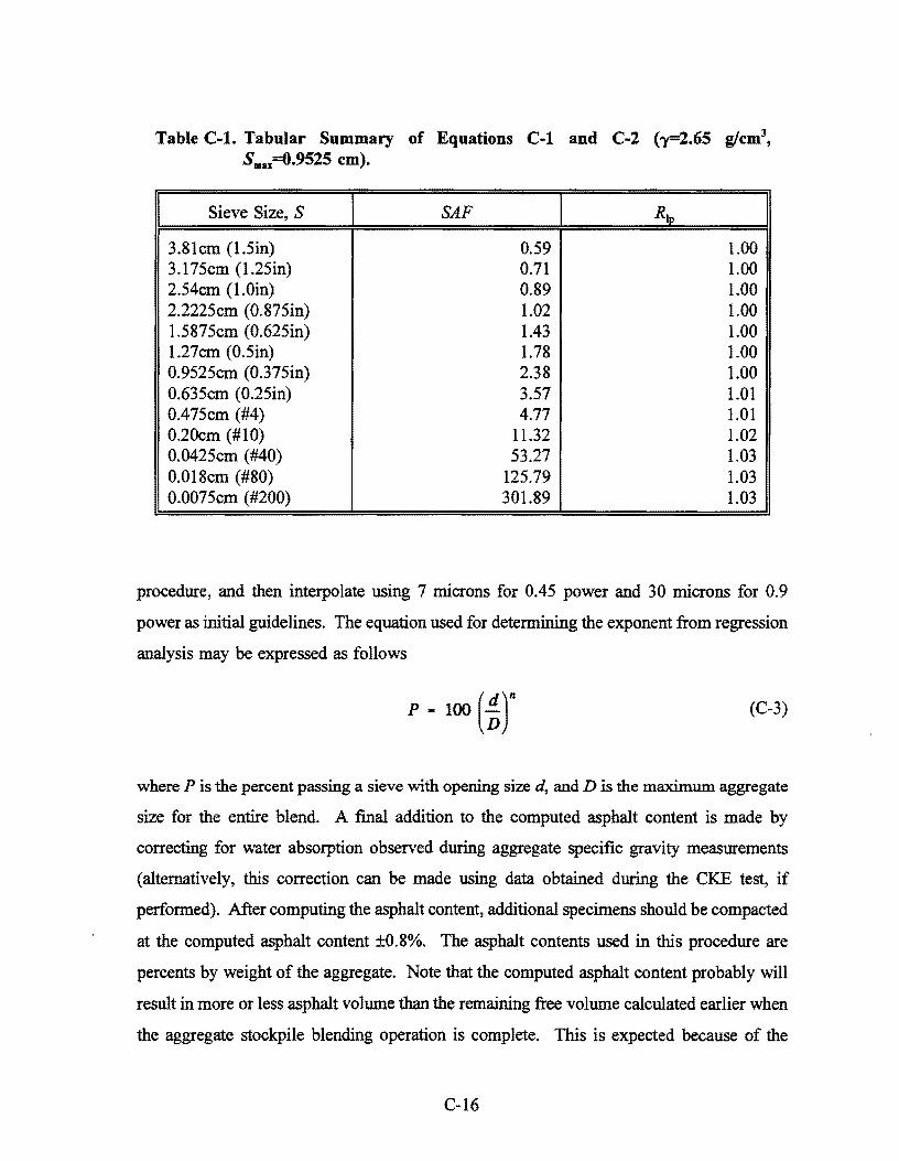
Table C-1. Tabular Summary of Equations C-1 and C-2 (')'=2.65 g/cm3,
smax=0.9525 cm).
Sieve Size, S SAF R1p
3.81cm (I.Sin) 0.59 LOO 3.175cm (1.25in) 0.71 1.00 2.54cm (l.Oin) 0.89 1.00 2.2225cm (0.875in) 1.02 1.00 l.5875cm (0.625in) 1.43 LOO 1.27cm (0.5in) 1.78 1.00 0.9525cm (0.375in) 2.38 1.00 0.635cm (0.25in) 3.57 1.01 0.475cm (#4) 4.77 1.01 0.20cm (#10) 11.32 1.02 0.0425cm (#40) 53.27 1.03 0.018cm (#80) 125.79 1.03 0.0075cm (#200) 301.89 1.03
procedure, and then interpolate using 7 microns for 0.45 power and 30 microns for 0.9
power as initial guidelines. The equation used for determining the exponent from regression
analysis may be expressed as follows
p _ 100 (~r (C-3)
where P is the percent passing a sieve with opening size d, and D is the maximum aggregate
size for the entire blend. A final addition to the computed asphalt content is made by
correcting for water absorption observed during aggregate specific gravity measurements
(alternatively, this correction can be made using data obtained during the CKE test, if
performed). After computing the asphalt content, additional specimens should be compacted
at the computed asphalt content ±0.8%. The asphalt contents used in this procedure are
percents by weight of the aggregate. Note that the computed asphalt content probably will
result in more or less asphalt volume than the remaining free volume calculated earlier when
the aggregate stockpile blending operation is complete. This is expected because of the
C-16

approximate nature of the computations (e.g., no integration is performed for individual
stockpile gradation and shape effects; air void content is not part of the design computation
at this time, and the selection of film thickness is somewhat subjective). If the computed
asphalt content minus 0.8% results in an asphalt volume that is greater than the available
free volume, it is suggested that a fourth asphalt content be included in the set of compacted
specimens. The fourth asphalt quantity would be (a) that which fills the available remaining
free volume while allowing for the desired air voids, or (b) the computed asphalt content
minus 1.6%, whichever is greater. It is suggested that agencies retain data on available free
volume, asphalt volume (both corrected and uncorrected for absorption), and air voids of
the compacted mix for use in developing a technique to reduce the number of compacted
mixtures in the mix design process if air void content is specified.
4. The following data and computations are provided as an example of the process.
Table C-2 summarizes the basic data on the aggregates and the measurements from vibration
tests with these aggregates. The volume calculation given in this table is computed after
vibrating the dry material in a suitable container. The interior dimensions of the container
are used in conjunction with the measured thickness of a surcharge plate (resulting in
approximately 1-2 k:Pa pressure simply to ensure that the vibration causes compaction and
the weight does not allow decompaction) to compute the volume of the material below the
surcharge after vibration (i.e., the average of three distance measurements from the top of
the container to the top of the surcharge plus the surcharge thickness, subtracted from the
total depth of the container when empty is the height of the aggregate plus air. Multiply
the height of the aggregate plus air by the internal cross sectional area of the container to
obtain the volume measurement). The weight of water listed in the table is for an
alternative method of measuring the void volume by filling to the average level of the
aggregate and computing the volume corresponding to the weight of water required to fill
to this level. The water method should not be used unless a correction is made for
absorption in the computations. The gradations of the individual components of the mix are
given in Table C-3.
Table C-4 presents the results of the fundamental calculations required to define the
stockpile blending proportions. First, the D50 size is computed for each stockpile by linearly
C-17

Table C-2. Example of Aggregate Data.
Stockpile Bulk % Volume2 ( cm3
) Weights (g) Specific Absorption1
Gravity1
1 2.630 1.91 Total: 3,027.65 Aggregate: 4,443 Aggregate: Water: 1,395
1,689.35 Air: 1,338.30
RAP 2.579 1.11 Total: 2,028.16 Aggregate: 3,614 Aggregate: Water: 601
1,401.32 Air: 626.84
1 Average of 3 measurements. 2 Average of 9 height measurements used in total volume computation (3 measurements after each of 3 vibration tests)
Table C-3. Component Material Gradations.
Sieve Size (cm) Percent Passing
Stockpile 1 RAP Rubber
3.81 100.00 100.00 100.00 3.175 100.00 100.00 100.00 2.54 100.00 100.00 100.00 2.2225 100.00 100.00 100.00 1.5875 100.00 100.00 100.00 1.27 100.00 100.00 100.00 0.9525 87.37 97.01 100.00 0.635 75.37 91.30 100.00 0.475 27.37 85.59 97.93 0.2 4.19 60.58 84.48 0.0425 2.38 32.23 3.95 0.018 1.99 16.53 1.32 0.0075 1.41 9.48 0.25
C-18

Table C-4. Weight Proportioning Calculations.
I Item I Stockpile I I RAP I Blend I Rubber I Dso 0.55 0.14 0.48 0.13 DMAXi 0.22 0.06 0.19 ----
Aggregate Wt (g) 4,443.00 2,384.98 6,827.98 ----Aggregate Vol 1,689.35 924.82 2,614.17 ----(cm3) 0.651 0.349 1.000 ----Weight Proportion
interpolating between the two sizes that bracket the 50% passing size. This number is
rounded to two decimal places in centimeters. Then the DMAXi size is computed as 0.4D50
assuming the elongated particle shape factor (rounded to two decimal places in centimeters
again). Once the decision has been made concerning how many of the available stockpiles
will be used, it is a relatively simple process to compute the weight proportions for the
blend. The process assumes that there are no significant interaction effects that would
preclude usage of the air volume data from vibrating individual stockpile materials in the
blend. The calculation sequence adheres to the following logic. Start with the largest
stockpile (#1) aggregate weight, aggregate volume and air volume from Table C-2. Proceed
down through the stockpiles as follows.
(a) From the vibration test, compute the fraction of the volume of the RAP stockpile
that is aggregate (1,401.32/2,028.16=0.691).
(b) Completely fill the available volume in stockpile I (1,338.51cm3) with the RAP.
From step (a), only 69. l % of the available volume will be filled with aggregate
which results in an aggregate volume and weight of RAP material of 924.82 cm3
and 2,384.98 g, respectively (the small difference in hand computed values from
the table is the result of more significant figures used in the spreadsheet program
used to compute these values).
C-19

( c) Any additional stockpiles can be used to fill the remaining free volume by
repeating steps (a) and (b). In this case, no other stockpiles are necessary.
(d) Total the aggregate weight (6,827.98).
(e) Compute the stockpile proportions (e.g., 2,384.98/6,827.98=0.349). This is the
blend recommended to ensure stone-on-stone contact with the stone skeleton
created by the virgin stockpile playing a significant role in the load carrying
capacity of the material.
Once the blend has been established, the final plant mix gradation is obtained by
simply proportioning the materials according to the laboratory sieve analysis and the
proportions of each size from step ( e) above and multiplying the result by the lab-to-plant
adjustment ratio, R1P. This has been done in the final gradation computation given in Table
C-5. In addition, computations of ln(d/D) and ln(P/100) have been performed for use in
regression analysis on a spreadsheet to compute n in Equation C-3 (if regression analysis
Table C-5. Data for Asphalt Content Determination.
Sieve Size Plant Gradation ln(d/D) ln(P/100) Surface Area (cm) (% Passing by (cm2
)
weight)
3.81 100.00 0.00 0.00 0 3.175 100.00 0.00 0.00 0 2.54 100.00 0.00 0.00 0 2.2225 100.00 0.00 0.00 0 1.5875 100.00 0.00 0.00 0 1.27 100.00 0.00 0.00 0.165426 0.9525 90.79 -0.29 -0.10 0.218201 0.635 81.68 -0.69 -0.20 1.196791 0.475 48.36 -0.98 -0.73 1.150033 0.2 24.41 -1.85 -1.41 1.309653 0.0425 13.16 -3.40 -2.03 3.22482 0.018 7.27 -4.26 -2.62 3.771168 0.0075 4.35 -5.13 -3.14 13.48976
C-20

tools are not available, use 0.0015 cm for the film thickness as an approximation). Using
the data shown in the table, and forcing the intercept to zero, linear regression on a
spreadsheet results in a value of 0.62 for n. Interpolating for film thickness between n=.45
(film thickness assumed to be 0.0007 cm), and n=0.9 (assumed film thickness 0.0030 cm)
results in a film thickness of 0.0016 cm for this gradation. With regard to film thickness,
it is noted that film thickness varies with the size particle, s9 the computed value is a crude
approximation of the average for the blend. Also, thicker films may be used as rubber
content increases. Concerning the role of fines, it has been suggested by other authors (e.g.,
Tunnicliff 1962) that fine particles with dimensions smaller than the film thickness often act
as extenders of the fluid binder.
To the surface area of the aggregate, the surface area of the rubber must be added.
By using the percent rubber in the RAP asphalt cement, the percent asphalt in the RAP, and
the estimated surface area of 150 cm2/g, the surface area of the rubber is found to be 0.576.
The total surface area of the blended material then becomes 25.1 cm2/g, which results in an
asphalt content of 4.02% by weight of the aggregate using the equation
(C-4)
where AC% is the percent asphalt by weight of the aggregate, SA is the total surface area
per gram, TF is the film thickness in cm, and Ya is the unit weight of asphalt (assumed to be
1.03 g/cm3 in this example). To this quantity, one must add a correction for absorption
which is accomplished by adding the absorptions for each stockpile. This is approximated
by multiplying the weight fraction of the stockpile by the water absorption (e.g., for
stockpile #1, 1.91*0.651=1.24). Finally, the total asphalt necessary is 4.02+1.63=5.65%.
The asphalt available from the RAP for this blend is 1.92%, which implies that the virgin
asphalt cement required is 3.73%.
5. The final step in designing the blend is to blend the asphalts to obtain suitable
binder properties. At this time, penetrations are used for selecting the asphalt blend.
(a) Compute the percent asphalt available from the RAP (1.92/5.65=34.0%). On
Figure C-1, move up from the baseline (0% CRM RAP AC) to 34% and draw
C-21

a horizontal line. 8
(b) Prepare the following 4 blends for penetration at 25°C (110°F):
1. 0% rejuvenating agent, 66% virgin AC, 34% CRM RAP AC,
2. 0% virgin AC, 66% rejuvenating agent, 34% CRM RAP AC,
3. 20% rejuvenating agent, 46% virgin AC, 34% CRM RAP AC, and
4. 20% virgin AC, 46% rejuvenating agent, 34% CRM RAP AC.
These four blends were selected to give a reasonably complete view of the
variation of the penetration of the blends along the CRM RAP AC = 34% line.
( c) At each point for which penetration measurements have been taken (i.e., at each
vertex and the four points from step b ), mark the point and label it with the
appropriate value of loguJ>en. Select the combination that has the desired
penetration (e.g., a 60 Pen material would be 1.778 on the chart) by interpolating
between the two nearest points. 9
( d) In addition to the desired penetration, it is also recommended that the
temperature sensitivity of the material be tested by conducting an additional
penetration test using the selected blend at 35°C (160°F) and at 25°C (110°F).
Compute Pfeiffer and van Doormaal' s slope, A, as
8The easiest way to understand this figure is to recognize that the scale for CRM RAP AC goes from 0 to 100 when going vertically from the baseline to the vertex. Each of the other two scales is interpreted in the same way, and this is easiest to see by simply rotating the page so that each legend is right side up in sequence.
9This technique essentially reduces to that used in ASTM D4887 if only two components are to be used. Although linear interpolation is used in this proposed procedure to find the final combination, it does not assume that the relationship between loguf'en and the percent recycling agent is linear as is done in the ASTM procedure with log10 Vis. It has been observed that, in many cases, the lines are not necessarily straight as implied by the ASTM procedure. The additional 5 penetration measurements should help refine the interpolation process, especially ifthe user elects to plot contour lines using all 7 data points. Of course, in the two component mix problem, a maximum of four penetrations would be conducted with only three of the four actually being used in the final analysis (e.g., the two ends of the rejuvenating agent = 0% baseline and the intersection of that line with the 34% CRM RAP AC line).
C-22

A log1o-Pen35 - log1o-Pen25
35-25
and the penetration index, PI, as
PI = 20-500A 1+50A
(C-5)
(C-6)
Most unmodified asphalts have a PI between +l and -1, with a value of below -2
indicating potential temperature susceptibility problems.
6. Perform an initial check on the effective utiliz.ation of the largest stockpile of
material (stockpile 1) and the compaction effort by computing the voids in the coarse
aggregate stockpile material in the compacted asphalt mixture. This computation is simply
the bulk specific gravity, Gbs, of the compacted mixture times the weight fraction of the
aggregate in the total mix times the weight fraction of the stockpile # 1 material. The result
of this calculation is the unit weight of the material from stockpile # 1 in the total mix; this
number should be greater than or equal to the unit weight of this material computed from
Table C-2 (4,443/3,027.65=1.467g/cm3).
7. Perform the mixture analysis test( s) desired. Either or both of the two tests are
recommended for performance analysis: (1) the axial creep test (Tex-231-F), or (2) the
repeated shear test. If axial creep is used, it is recommended (optional) that radial strains
be measured and/or multiple confining pressures be used so that stone-on-stone contact can
be reevaluated along with the analyses for long term performance. If repeated shear testing
is performed, it should be done at constant height, and the axial load required to keep the
height constant should also be recorded for the stone-on-stone contact analysis. Poisson's
ratio is expected to equal or exceed 0.5 for mixes with good stone-on-stone contact.
Materials with good stone-on-stone contact will have higher axial loads to maintain height
in the shear test. The previous two statements should only be interpreted as identifying
superior mixtures if the other portion of the analysis indicates that long term performance
C-23

is acceptable (i.e., impending failure can also be accompanied by high Poisson's ratios and
high axial loads in the shear test under certain circumstances).
8. If the analysis procedure indicates that the mixture will not perform adequately,
the following suggestions are offered for correction of the problem. Remove any stockpile
that has the same D50 size as the DMAXi size of the next larger stockpile, change the
compaction·effort to increase the unit weight of the mix (within the limits of what available
compaction equipment will realistically be able to accomplish at the site, which will also be
affected by characteristics of the platform against which the material will be compacted),
and modify the asphalt with materials such as fillers or polymer modifiers (which may not
cost effectively enhance resistance to rutting). If the problem is due to breakdown of the
·aggregate during mixing and/or compaction, a different parent material source for the
aggregate must be selected. The performance evaluation does not evaluate moisture effects.
This can be done through surface chemistry related tests and/or water permeability tests with
leachate analysis.
9. If moisture effects are not measured, pick the highest asphalt content that gives the
desired indication of long term performance from step 7 (minus the expected variability of
asphalt content at the plant). If moisture effects are measured, select the lowest asphalt
content that meets both moisture and performance requirements (plus the plant variability).
C-24
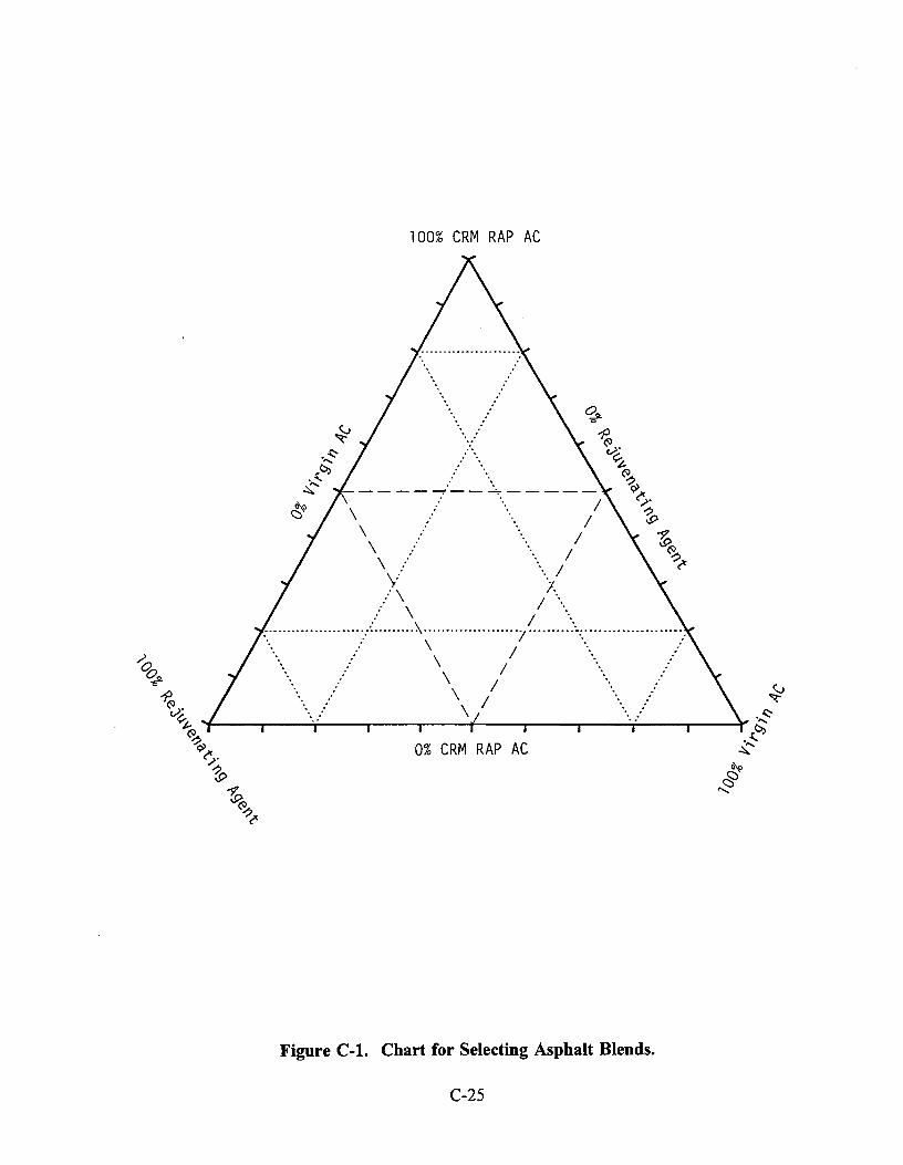
100% CRM RAP AC
. . ----~--~-----. .
\ I \ ! I
\ : I " I \ . ..
\ : "·I / \ 1.
\ I \.
-;, \------ _:/ \~ --- / \::- -- :: l:2s \ I o~ / \ I ~
~- : \ I " ~~ "'1-~---,r--~~._r .. ~~r-~--.-~~+-~---..~~-.--~__:·~·~~-r-~~·~ ~ ~
9> 0% CRM RAP AC .;._" 0· ~ ~ ~ ~ ~?
I<
Figure C-1. Chart for Selecting Asphalt Blends.
C-25


APPENDIX D - ALTERNATIVE USES OF RECYCLED RUBBER
To address the problem of waste tire disposal to satisfactory utilization levels,
alternative use of waste rubber should be under constant evaluation. The uses of tire rubber
can be divided into three broad categories: energy conversion, whole tire applications, and
shredded rubber applications. Suggestion of the following alternative uses is based on
experiences reported by state agencies across the U.S. which have been documented by Epps
(1994). The State of Minnesota estimates that it will exhaust its supply of waste tires within
a few years primarily because of high volume use as fuel and as lightweight fill.
ENERGY CONVERSION
Tires are currently being burned as a fuel source. Tire Derived Fuel (TDF) is either
produced in a facility solely dedicated to tires-to-energy operations, or is more directly used
in electric power generation, production of cement in cement kilns, and for paper milling.
WHOLE TIRE APPLICATIONS
Retaining Walls
Tires are placed in parallel rows and backfilled with permeable material and covered
behind, under, and over the tires with engineering fabric to prevent soil erosion. A thick
layer of native soil is placed on top of the last layer of engineering fabric to encourage
vegetation.
Impact Attenuators
Vehide impact attenuators can be constructed using tires anchored together and filled
with sand.
D-1

Safety Hardware
Whole tires can be used as bases for tubular traffic control markers and bases for
vertical panel supports.
Fills and Embankments
Whole tires can be laid in a single or double layer over an existing roadbed as fill
material in areas where the naturally occuring soil is peat or other soft soil.
Windbreaks
To reduce blowing sand and wind damage to young seedling trees in desert areas,
woven tire walls and mats of tires can be constructed.
Culverts
Culverts can be built from tires bound together with steel reinforcing bars.
SHREDDED RUBBER APPLICATIONS
Lightweight Fill and Embankment
Tire chips are placed on excavated soil and compacted. A filter fabric is placed on the
chips followed by a depth of earth fill.
Drainage Layer
Existing base material can be replaced with rubber chips laid in thicknesses of several
centimeters covered by a layer of gravel. The tire chips can prevent capillary rise of ground
water and thus minimize base contamination from the underlying subgrade.
D-2

Membranes
Membranes have been made with asphalt rubber binders and used for pond liners and
to control moisture content in swelling clay soil subgrades.
Miscellaneous
Playgrounds, sidewalks, horse stall bedding, and potting soil amendments are some
additional uses of the material. It is being considered for structural components and signs.
Noise attenuating barrier walls can be constructed in high noise areas using the rubber as
the attenuating medium in the structure.
D-3