THE EFFECT OF LENGTH ON TENSILE STRENGTHPARALLEL-TO—GRAIN IN STRUCTURALLUMBER_

Karen L. Shcwalter

Thesis submitted to the Faculty of the

V Virginia.Polytechnic'Institute and State University

4 in partial fulfillment of the requirements for the degree of

· _ Master of ScienceE in

Agricultural Engineering '

APPROVED:

» Frank E. Woeste, Chairman

E KWJL c· DA!-Z Ä12.,%/1.KennethC. Diehl .Theo A. Dillaha

July 8, 1985 ‘

Blacksburg, Virginia —

OI 4 ll °’¤

T «T\_ .

THE EFFECT OF LENGTH ON TENSILE STRENGTHPARALLEL-TO-GRAIN IN STRUCTURAL LUMBFR p

l

byKaren L. Showalter

Frank E. Woeste, Chairman _l

Agricultural Engineering

. (ABSTRACT)0

Two sizes (2x4 and 2x10) and two grades (2250f-1.9E and' No. 2 KDl5) of Southern Pine lumber having three different

.4_ test span lengths of 30, 90 and 120 inches were tested in

_

tension parallel-to-grain. Results obtained from the tests

indicated that the tensile strengths of the 30-inch test

specimens were significantly higher than the tensile

strengths of the 90- and 120-inch test specimens.

· A tensile strength-length effect model was developed for

V' generating tensile strength ‘values of lumber taking thel

length effect into consideration. The model generates

tensile strength values for lumber longer than 30 inches inh _

multiples of 30 inches, ie. 60-, 90- 120-inch lengths. The

two sizes and two grades of Southern Pine lumber formed the

data base for developing the model.

The tensile strength-length effect model utilized an MOE ·

_ variability model which generated serially correlated MOE's

along 30-inch segments for a piece of lumber using a second-

order Markov model. The segment MOE values were then used

in a first-order Markov model to generate serially correlated

tensile strength residuals for each 30-inch segment. The

segment MOE values and the segment tensile strength residuals

were then inputted into a weighted least squares regression

to obtain the tensile strength parallel-to-grain for each

30-inch segment. The tensile strength of the generated pieceU

of lumber was then determined using the weakest·link concept;

the minimum segment tensile strength value was selected as

the tensile strength of the generated piece of lumber.

Acknowledgements _ liv

TABLE OF CONTENTS

CHAPTER I. INTRODUCTION 1

V CHAPTER II. REVIEW OF LITERATURE ...... . . . . 42.1 Weakest-Link Applications in Lumber ....... 6

2.1.1 Bending Strength ......._....... 8

2.1.2 Tensile Strength Perpendicular-to-Grain . . . 9

2.1.3 Shear Strength ............... 1O

2.1.4 Tensile Strength Parallel-to—Grain ..... 11

2.2 Stochastic Models . . . . ............ 122.2.1 First Order Markov Process ......... 12

2.2.2 Higher Order Markov Model .......... 13

2.3 Weighted Least Squares Regression Model ..... 16

CHAPTER III. EXPERIMENTAL DESIGN .......... 18

3.1 Description of Material ............. 18

3.1 Conditioning ......_ ........... 19

3.1.2 Assignment to Treatment Groups ....... 21

3.1.3 Measurement of MOE ............. 25

3.1.4 Tension Testing ............... 26

3.2 Data Analysis .................. 28

CHAPTER IV. MODEL DEVELOPMENT ..... . ...... 46

4.1 Development of a Model Assuming Independent Segments 47

Table of Contents v

4.2 Development of a Model of Correlated Segments . 61

4.2.1 Generation of Segment MoE's ......... 61

4.2.2 Weighted Least Squares Regression ...... 68

4.2.3 Specimen Tensile Strength .......... 78

4.3 Preliminary Validation Results ......... 79

4.3.1 Independent Segments Model ......‘. . . 79

4.3.2 Correlated Segments Model .......... 8O

CHAPTER V. MODEL REFINEMENTS ............ 86

5.1 Modeling of the Residual ............ 86

5.2 Generation of Residuals ............. 89

CHAPTER VI. RESULTS ................. 93

CHAPTER VII. APPLICATION OF THE LENGTH EFEECT MODEL 115

7.1 Development of a Tensile Strength Length Adjustment 115

7.2 Applications of the Tensile Strength Length Ad-1

justment ..................... 129

CHAPTER VIII. SUMMARY AND CONCLUSIONS ....... 132

8.1 Summary .................... 132

8.2 Conclusions .................. 133

APPENDIX A. PROGRAM LISTING OF THE MODIEIED MOE VARI-

ABILITY MODEL. .................. 136

Table of Contents vi

APPENDIX B. PROGRAM LISTING OF THE TENSILEL

STRENGTH—LENGTH EFFECT MODEL. ........... 14O

REFERENCES ..................... 145

VITA ..................... . . . 147

Table of Contents vii

LIST OF TABLES V

Tablepage

3.1 The "regraded" lumber groups, their allowablebending stresses and the number of specimensin each group. . . .°............. 20

3.2 The number of specimens in each grade group andtreatment group of visually graded 2x4 areshown. .................... 22

3.3 The number of specimens in each grade group andtreatment group of visually graded 2xlO areshown. .................... 23

3.4 Required arrangement of tensile specimens in thetensile grips. ................ 27

3.5 Mean tensile strength in psi of visually graded2x4 lumber sample. .............. 29

3.6 Mean tensile strength in psi of visually graded2xlO lumber sample............... 30

3.7 Mean tensile strength in psi of 2250f—1.9E lumber. 31

3.8 Coefficient of variation of the tensile strengthin visually graded 2x4 lumber sample...... 37

3.9 Coefficient of variation of the tensile strengthin visually graded 2xlO lumber sample. .... 38

3.10 Coefficient of variation of the tensile strengthof the 2250f-1.9E lumber............ 39

3.11 Summary of hypothesis test illustrating thecorrelation of the ultimate tensile stress insegments "l" and "4" of the 30-inch groups atthe 0.05 significance level. ......... 45

4.1 The minimum and maximum 30·inch segment MOE valuesfor each grade and size group used in thedevelopment of the MOE variability model (Klineet al, 1985).................. 63

viii

5.1 The estimated lag-3 serial correlation and thecalculated lag-1 serial correlation for eachsize and grade group.............. 90

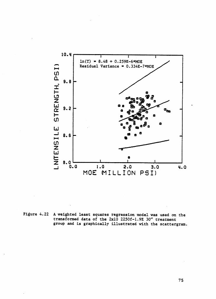
6.1 Listing of the eight groups of tensile strengthvalues simulated by the tensile strength-length effect models.............. 94

6.2 Lag—3 serial correlation of tensile strength bysize and grade................. 112

6.3 Fifth percentile values of tensile strength inpsi by size and grade. ............ 114

7.1 Fifth percentile tensile strength and lengthadjustment, Y, for 2x4 225f·1.9E Southern Pine. 119

7.2 Fifth percentile tensile strength and lengthadjustment, Y, for 2x10 225f·1.9E SouthernPine...................... 120

7.3 Fifth percentile tensile strength and lengthadjustment, Y, for 2x4 No. 2 KD15 SouthernPine...................... 121

7.4 Fifth percentile tensile strength and lengthadjustment, Y, for 2xlO No. 2 KD15 SouthernPine...................... 122

7.5 Estimated parameters A, B, and C of Equation 2for the tensile length adjustment model. . . . 124

ix

LIST OF FIGURES

Figure ·a e

_ 3.1 Location of four 30—inch segments for MOEmeasurements and the loading configuration forSegment "1". ................. 25

3.2 Mean tensile strength of the 2x4 2250f-1.9E MSRSouthern Pine versus length of the test span. . 32

3.3 Mean tensile strength of the 2xlO 2250f-1.9E MSRSouthern Pine versus length of the test span. . 33

3.4 Mean tensile strength of the 2x4 No. 2 KD15· Southern·Pine versus length of the test span. . 34

p 3.5 Mean tensile strength of the 2xlO No. 2 KD15Southern Pine versus length of the test span. . 35

3.6 5th percentile tensile strength of the 2x42250f-1.9E MSR Southern Pine versus length ofthe test span. ................ 40

3.7~ 5th percentile tensile strength of the 2xlO2250f-1.9E MSR Southern Pine versus length ofthe test span. ........‘. ....... 41

3.8 5th percentile tensile strength of the 2x4 No. 2KDl5 Southern Pine versus length of the testespan. ..................... 42

3.9 5th percentile tensile strength of the 2xlO No. 2KDIS Southern Pine versus length of the testspan. ..................... 43

4.1 A lognormal distribution is superimposed on thehistogram of the tensile strength of the 2x42250f-1.9E MSR 30" treatment group. ...... 49

4.2 A lognormal distribution is superimposed on thehistogram of the tensile strength of the 2xlO2250f-1.9E MSR 30" treatment group. ...... 50

x

4.3 A lognormal distribution is superimposed on thehistogram of the tensile strength of the 2x4No. 2 KD15 30" treatment group. ........ 51

4.4 A lognormal distribution is superimposed on thehistogram of the tensile strength of the 2xlONo. 2 KD15 30" treatment group. ........ 52

4.5 The probability distribution with n=3 issuperimposed onto the histogram of theultimate tension of the 2x4 2250f-1.9E MSR 90"treatment group. ............... 53

4.6 The probability distribution with n=3 issuperimposed onto the histogram of the

„ ultimate tension of the 2xlO 2250f—1.9E MSR90" treatment group. «.„............ 54

4.7 The probability distribution with n=3 is ·superimposed onto the histogram of theultimate tension of the 2x4 No. 2 KD15 90" »treatment group. _............... 55

4.8 The probability distribution with n=3 issuperimposed onto the histogram of theultimate tension of the 2xlO No. 2 KD15 90"

A treatment group- ............... 56

4.9 The probability distribution with n=4 issuperimposed onto the histogram of theultimate tension of the 2x4 2250f·l.9E MSR120" treatment group. ............. 57

4.lO The probability distribution with n=4 issuperimposed onto the histogram of theultimate tension of the 2xlO 2250f·l.9E MSR120" treatment group. ............. 58

4.11 The probability distribution with n=4 issuperimposed onto the histogram of theultimate tension of the 2x4 No. 2 KD15 120"treatment group. ............... 59

4.12 The probability distribution with n=4 issuperimposed onto the histogram of theultimate tension of the 2xlO No. 2 KD15 l20"treatment group. ............... 6O

xi

4.13 A lognormal distribution is superimposed onto thehistogram of MOE values measured from the 2x4 ‘2250f—1.9E MSR 30" treatment group. ...... 64

4.14 A lognormal distribution is superimposed onto thehistogram of MOE values measured from the 2xlO ’2250f-1.9E MSR 30" treatment group. ...... 65

4.15 A 3-parameter Weibull distribution issuperimposed onto the histogram of MOE valuesmeasured from the 2x4 No. 2 KD15 30" treatmentgroups.. ............... 66

· 4.16 A 3-parameter Weibull distribution is _superimposed onto the histogram of MOE valuesmeasured from the 2xl0 No. 2 KD15 30"treatment groups. ....<. .......... 67 _

4.17 Results of weighted least squares regression 'analysis on the 2x4 2250f—l.9E 30" treatmentgroup of the tensile strength—MOE relationship. 70

. 4.18 Results of weighted least squares regressionanalysis on the 2xlO 2250f-1.9E 30" treatmentgroup of the tensile strength-MOE relationship. 71

4.19 Results of weighted least squares regressionanalysis on the 2x4 No. 2 30" treatment groupof the tensile strength-MOE relationship. . . . 72

A4.20 Results of weighted least squares regression

analysis on the 2xlO No. 2 30" treatment groupof the tensile strength—MOE relationship. . . . 73

4.21 A weighted least squares regression model wasused on the transformed data of the 2x42250f-1.9E 30" treatment group. ........ 74

4.22 A weighted least squares regression model wasused on the transformed data of the 2xlO2250f-1.9E 30" treatment group. ........ 75

4.23 A weighted least squares regression model wasused on the transformed data of the 2x4No. 2 30" treatment group. .......... 76

I pxii

4.24 A weighted least squares regression model was— used on the transformed data of the 2xlO —No. 2 30" treatment group. .......... 77

4.25 The histogram of the ultimate tension of the 2x4. 2250f-1.9E 90" treatment group with the

· correlated segment model probability curvesuperimposed. ................. 81

4.26 The histogram of the ultimate tension of the 2x42250f-1.9E l20" treatment group with thecorrelated segment model probability curvesuperimposed. ................. 82

4.27 The histogram of the ultimate tension of the 2x4No. 2 90" treatment group with the correlatedsegment model probability curve superimposed. . 83

4.28 The histogram of the ultimate tension of the 2x4No. 2 l20" treatment group with the correlatedsegment model probability curve superimposed. . 84

5.1 A simulated scattergram of the tensile strengthMOE relationship. ............... 87

6.1 A lognormal distribution is superimposed onto thehistogram of the generated tensile strengthvalues from the length effect model of the 90"2x4 2250f-1.9E MSR Southern Pine. ....... 95

6.2 A lognormal distribution is superimposed onto thehistogram of the generated tensile strengthvalues from the length effect model of the120" 2x4 2250f-1.9E MSR Southern Pine. .... 96

6.3 A lognormal distribution is superimposed onto thehistogram of the generated tensile strengthvalues from the length effect model of the 90"

1 2xlO 2250f-1.9E MSR Southern Pine. ...... 97

6.4 A lognormal distribution is superimposed onto thehistogram of the generated tensile strengthvalues from the length effect model of thel20" 2xlO 2250f-1.9E MSR Southern Pine. .... 98

7 xiii

6.5 A lognormal distribution is superimposed onto thehistogram of the generated tensile strengthvalues from the length effect model of the 90"2x4 No. 2 KD15 Southern Pine. ......... 99

6.6 A lognormal distribution is superimposed onto thehistogram of the generated tensile strengthvalues from the length effect model of the120" 2x4 No. 2 KDl5 Southern Pine. ...... 100

6.7 A lognormal distribution is superimposed onto thehistogram of the generated tensile strengthvalues from the length effect model of the 90"2x10 No. 2 KD15 Southern Pine. ........ 101

6.8 A lognormal distribution is superimposed onto thehistogram of the generated tensile strengthvalues from the length effect model of the120" 2x10 No. 2 KD15 Southern Pine. ..... 102

6.9 The model generated tensile strength-lengtheffect probability curve is superimposed ontothe histogram of ultimate tension of the 2x42250f-1.9E MSR 90" treatment group. ..... 104

6.10 The model generated tensile strength-lengtheffect probability curve is superimposed ontothe histogram of ultimate tension of the 2x42250f-1.9E MSR 120" treatment group. ..... 105

6.11 The model generated tensile strength-lengtheffect probability curve is superimposed ontothe histogram of ultimate tension of the 2xlO2250f-1.9E MSR 90" treatment group. ..... 106

6.12 The model generated tensile strength-lengtheffect probability curve is superimposed ontothe histogram of ultimate tension of the 2xl0

_ 2250f-1.9E MSR 120" treatment group. ..... 107

6.13 The model generated tensile strength-lengtheffect probability curve is superimposed ontothe histogram of ultimate tension of the 2x4No. 2 90" treatment group. .......... 108

xiv

6:14 The model generated tensile strength-lengtheffect probability curve is superimposed onto Athe histogram of ultimate tension of the 2x4No. 2 l20" treatment group. ......... 109

6.15 The model generated tensile strength-lengtheffect probability curve is superimposed ontothe histogram of ultimate tension of the 2x10No. 2a9o“ treatment group. .......... 110

6.16 AThe model generated tensile strength-lengtheffect probability curve is superimposed ontothe histogram of ultimate tension of the 2x10

» No. 2 120" treatment group. ......... 111

7.1 Length adjustment, Y, for 2x4 2250f-1.9E SouthernPine. .................... 125

7.2 Length adjustment, Y, for 2x10 2250f-1.9ESouthern Pine- ................ 126

7.3 Length adjustment, Y, for 2x4 No. 2 KD15 Southern„ ‘ Pine. .................... 127

7.4 Length adjustment, Y, for 2x10 No. 2 KD15Southern Pine. ................ 128

Aßä ‘ „

* xv

CHAPTER I. INTRODUCTION

By current design practice (National Forest Products

Association, 1982), trusses of all lengths have the same im-

plied safety. Failure experience, however, indicates that

long-span trusses have a higher incidence of failure than

short-span trusses. While there are many factors involved,

it is believed that a decreasing tensile strength with an

increase in the lower chord length may be one factor. Be-

cause of the poor performance, many manufacturers will not

design or produce trusses longer than 60 to 80 feet. An em-

pirical evaluation of the effect of length on tensile l

strength will provide the basis for a model that can be used

for safety adjustments in long-span truss design.

A tensile length model will be useful for several addi-u

tional applications:

1. During a recent cooperative research project between

Virginia Tech and the U. S. Forest Products Laboratory (EPL)

(Bender, 1980), a computer—based model was developed for the

reliability of glued-laminated (glulam) beams at room tem-

perature and when exposed to fire.. In the process of cali-

„ brating the room temperature portion of the developed model

with some existing glulam beam data, it was discovered that

, adding a length adjustment significantly improved the

strength comparisons between the model and available data.l

l

· The length adjustment was included to account for the dif-

ference in the length of the tensile specimens used as data

input for the model, and the length of the various test beams

subject to maximum moment.

Unpublished test results from Trus Joist Corp. indicate

a signicant reduction in tensile strength with increasing

lengths of MICRO=LAM (Trus Joist Corp., 1979). It was hy-

pothesized that lumber, with larger defects, should be more

sensitive to length„ Since no tensile strength length ad-

justment was known for structural lumber, it was assumed that

lumber behaved as a weakest link type structure when stressed

”in tension parallel to grain (Bender, 1980).

Bohannan (1966 a,b) studied the effect of volume on the

bending strength of laminated timber beams. The volume ef-

fect is based on the "weakest-link theory." In applying

weakest link theory to wood beams the volume is replaced by

the beam aspect area (Liu, 1981). To obtain bending strength

results for beams of different lengths and depths, the stress

function is integrated over the area of the beam. An alter-

nate approach to integrating a stress function over an area

is to evaluate the bending strength of the laminated beam by

Monte Carlo simulation (Bender, 1980). The stress in each

piece of lumber between end joints is calculated and compared

to a strength. value. Hence tensile strength. values for

pieces of lumber of various lengths are needed.

2

2. In the Canadian glulam computer simulation model

(Eoschi, 1980), 6-inch—long finite elements are used: hence

tension information on 6-inch lengths of lumber is needed for

that model. Six-inch lengths of full-size lumber are diffi-

cult, if not impossible to test in tension parallel-to-grain.

As a compromise the length model can be used to predict the

30-inch tensile strength.‘

3. The In-Grade testing program provides data on lim-

ited lengths. If a length tensile model is verified, it can

be used to make adjustments to In-Grade tensile data.

Tensile strength data from various studies have been col-

lected on specimens of different lengths. Data to adjust forldifferent gage lengths would be useful in comparing tensile

strength results.

The objectives of this study were to:

1. Determine if there is a length effect on tensile

strength parallel-to-grain in two sizes (2x4 and

2x10) and two grades (2250f-1.9E and No. 2 KDIS)

of Southern Pine lumber.

2. Develop a length effect model for tensile strength

parallel-to-grain for the two sizes and two grades

of Southern Pine lumber.

3. Demonstrate the application of the tensile

strength-length effect model.

3

CHAPTER II. REVIEW OF LITERATURE

In current design practice, the stiffness of a piece of

lumber indicates some average stiffness value for the whole

piece and the strength indicates the stress capacity of the

whole piece of lumber. Because a piece of lumber usually

contains defect areas such as knots and grain deviations

along the piece, presumably a more accurate representation

of lumber strength or stiffness would include variability in

strength or stiffness with size. Several researchers have

documented a variability of strength of a wood member with

size.

Buchanan (1983) reports that the strength of wood

flexural members decreases as the size of the test specimen

V increases. Bohannan (1966) also confirms that bending

strength of wood beams decreases as the size of the beam in-

creases. Bohannan‘s results for clear, straight—grained,

Douglas-fir beams having sizes ranging from 1 inch deep by

14 inches long to 31-1/2 inches deep by 48 feet long shows a

decrease in the average modulus of rupture with increasing

length and depth.V

Recently, Kunesh and Johnson (1974) carried out axial

tension tests on clear Douglas-fir lumber and identified a

pronounced size effect, with the average strength cxf 2xlO

lumber being only 81% of the strength of 2x4 lumber. Since

4

all specimens were 12 feet long, no conclusions regarding a

length effect were possible. Buchanan (1983) also cites4

other investigations where a trend of increasing tensile

strength with decreasing size was identified.

A size effect on shear strength of wood beams was noted

by Liu (1980) during a study on glued—laminated 0ouglas·fir

beams. Liu's test results showed that the mean failure shear

stress decreased with increasing volume.

Barrett (1974) reports that a similar size effect exists

when testing tensile strength perpendicular-to-grain of

Douglas-fir. Barrett's report consists of tensile strength

results for uniformly loaded glued-laminated Douglas-fir

blocks of commercial material for clear Douglas—fir blocks

loaded perpendicular-to-grain. In both cases, the average

strength of the material decreases with increasing volume.

More specifically, the results also show a decrease in the

. average tensile strength when only the length is increased.

The following three sections describe models which can

be used to aid in the explanation of the size effect on

strength of lumber specimens. The first section discusses

Weibull's weakest link theory. Several applications of the

weakest link theory are provided. The second section de-

scribes the use of stochastic models to model the variability

of strength and stiffnessxhn a lumber specimen. The final

section discusses a regression approach used by (Woeste et

15

al, 1979) to model and generate by the computer a compatible

set of strength and stiffness values.

2.1 WEAKEST-LINK APPLICATIONS INLUMBERThe

relationship between the size and strength of a wood

member has been the subject of research for many years. It

is apparent that as size increases in a wood member the

strength of the member decreases. Assuming that wood is a

perfectly brittle material, that is, a material in which

total failure occurs when fracture occurs at the weakest

point, the size effect can be explained by the statistical

theory of material strength, or, the "weakest-link theory"

(Weibull, 1939).

According ‘¤¤ Weibull (1939), the probability that a

chain of n links will have strength greater than or equal to .

X is given by:

- _ ¤ =1 - E¤(x) - [1 F(x)] Sn (2.1)

where Fn(x) is the probability distribution of strength for

chains of n links, and Sn is the survival probability. Tak-

ing logarithms:

ln[1 - F¤(x)] = —B = n*ln[1 - F(x)] (2.2)

_ Generally, the stress distribution within a body varies

with position. In this case, the value of B becomes

6

B = —{§n(x)dv (2.3)

where n(x) = ln[l-E(x)] from Equation 2.2. The form of the

function, n, must fit the cumulative distribution of strength

and describe the strength property being investigated.

Bohannan (1966) used the material function

n(x) = kxm (2.4)

in which k and m are material constants, in his study of the

size effect on bending strength. Barrett (1974) described

the material function to be

n(x) = l(x - xl)/mlm (2-5)

where xl is an arbitrarily lower limit or minimum strength,

m and x„ are material properties, m being a dimensionless

"shape parameter" and x„ being a "scale parameter" with unitsof stress. Assuming xl = O (Barrett, 1974), let (1/x„)m = k

and Equation 2.5 is the same as Equation 2.4.

Substitution of Equations 2.3 and 2.5 into Equation 2.2

gives the cumulative distribution function (CDE) of strength

to„be

E(x) = 1 - exp(-B) = 1 — exp[-f§(x/x„)mdv] (2.6)

If the stress distribution is assumed to be uniform then,

E(x) = 1 — exp(-B) = 1 — exp[-V(x/x„)m] (2.7)

7

which is the two-parameter Weibull distribution.

The "weakest-link theory" has been used in many appli-

cations to explain the size effect on strength of lumber,

mainly in the form of the two-parameter Weibull distribution

· (Equation 2.7). The following sections discuss the applica-

tion. of Vthe "weakest-link theory" on different strengthproperties.

2.1.1 BENDING STRENGTH

Bohannan (1966) used the statistical theory of strength

of materials to explain the relationship between size and

bending strength of wood members. Using the linear stress

theory to determine the stress distribution of failure,

Bohannan found the CDE for a beam with uniform volume under

two-point loading. The theoretical CDE was compared to an

observed CDE of three sets of data of clear straight-grained

Douglas-fir. The comparison showed some disagreement between

theory and the observed data.U

. V

A modified statistical strength theory was then derived

to better explain the size effect on bending strength in wood

members with uniform volume (Bohannan, 1966). By rational-

izing that the size effect on modulus of rupture is inde-.

pendent of the beam width, Bohannan developed an expression

for the CDE of bending strength dependent only on length and

depth of the beam. Comparing the theoretical and exper-

· 8

imental modulus of rupture using the same data showed rea-

sonably good agreement between theory and observed data

(Bohannan, 1966). _

. According to Liu (1981), the "weakest-link theory" can

also be used to analyze the size effect on bending strength

of tapered wood beams under arbitrary loading conditions.

Like Bohannan (1966), Liu adopted the linear bending stress

distribution to determine the CDF of bending strength. Liu

also developed the analysis of the size-strength relationship

of wood beams by considering only the aspect area as an ef-

fect on the bending strength. ‘

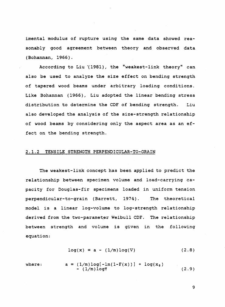
2.1.2 TENSILE STRENGTH PERPENDICULAR-TO-GRAIN

The weakest—link concept has been applied to predict the

relationship between specimen volume and load-carrying ca-

pacity for Douglas-fir specimens loaded in uniform tension

perpendicular—to-grain (Barrett, 1974). The theoretical

model is a linear log-volume to log-strength relationship

derived from the two—parameter Weibull CDF. The relationship

between strength and volume is given in the followingAequation:log(x)

= a · (1/m)log(V) (2.8)

where: a = (1/m)log[-1n(1—F(x))] + log(x„) .- (1/m)logY (2.9)

9

Y = constant depending on stress distributionand shape parameter, m _

The validity of the weakest link model was tested using the

results of tests on uniformly loaded Douglas-fir specimens.

The hypothesis that the weakest-link concept applies was ac-

cepted on the basis of the high coefficients of determination

obtained by least-sguares regression relating log-volume to

log-strength (Barrett, 1974).

2.1.3 SHEAR STRENGTH

Liu (1980) developed a model to describe the size effect

on shear strength in wood members by applying Weibull's sta-

tistical theory (1939). Assuming that the shear stresses are

uniformly distributed over a uniform volume, Equation 2.3

becomes

B = BV(x„/W„)m (2.10)

in which

Wu = %k(¤)%lF(r¤ + 1)/1”(m + 3/2)]-1/m

where F = the Gamma function;B is based on the shear force diagram

Substituting Equation 2.10 into Equation 2.6 gives the CDE

F(x) = 1 - exp[-BV(x/W„)m] (2.11)

10

The data set used to test and compare to the weakest- .

link model was shear failure results of 5 samples of glued-(

laminated Douglas-fir beams. A comparison of the theoretical

model to the observed data provided adequate evidence that

the weakest-link analysis interprets the size effect in shear

strength (Liu, 1980).

2.1.4. TENSILE STRENGTH PARALLEL-TO-GRAIN

Poutanen (1984) discusses the possibility of a length

effect on tensile strength parallel-to-grain in lumber. Al-

though he does not have data to verify the length effect, he

theoretically claims that an increased beam length results

in a decrease in tensile strength. Assuming that a defect

has cumulative strength distribution function F, and the wood

member has n defects, Poutanen describes the probability for

survival at stress level cl as:

P1 = (1 — F(¤1))° (2-12)

·If size is increased k times, the number of defects increases

r times. Assuming k = r when only the length is increased,

the probability of survival becomes

· kPa = (1 ' F(°z)) n (2·l3)

at stress level cz. Since all sizes fail with equal proba-

bility, P2 == P1, which implies E(c2)<F(c1). Subsequently,

11

if F(oz)<F(o,), then ¤2<c1 which implies that the member with

increased length is weaker in tension Pparallel-to-grainA

(Poutanen, 1984).

2.2 STOCHASTIC MODELS

It is reasonable to assume that lumber exhibits serialcorrelation; ie, that the strength or stiffness in one seg-

ment is correlated to the strength or stiffness at the pre-

vious segment. Lag-k serial correlation, pk, is the

correlation between an observation at one interval length and

an observation at k previous intervals. A Markov process is

one stochastic model that generates values for each segment

while preserving the significant serial correlation between

segments.2.2.1

FIRST ORDER MARKOV PROCESS

A first order Markov process can be used to model a

stochastic series if the serial correlation for lags greater

than one are not important. Haan (1977) defines a first or-

der Markov process by the equation

XM1 = Mx · ¤1(Xi · Mx) (2·l‘%)+ ··= P <1 · PHäi+1x

‘

where: xi = the value of the process atsegment i

~ 12

ux = the mean of Xox = the standard deviation of X 7

P1 = the first-order serial correlation

ti+1 = standard normal deviate, N(O,1)

This model assumes X to be from a normal distribution with

mean ux, variance oxz, denoted by N(ux, cx'), and first-order

serial correlation pl. It is also assumed that tt+l is in-dependent of Xi. Under these assumptions, this model gener-

ates synthetic events that preserve the mean, standard

deviation, and first-order serial correlation.

When the first-order Markov model cannot assume that the

process is stationary in its first three moments, it is pos-

sible to generalize the model to account for Variation be-

tween segments. If the mean, variance or serial correlation

Varies between segments the first-order Markov model becomes

*1+1'7 _2+ti+1¤x,i+l(l P1 )

Again, this model assumes X to be from a normal distribution

(Haan, 1977).

2.2.2 HIGHER ORDER MARKOV MODEL

If the serial correlation for lags greater than one are im-

portant the model given by Equation 2.14 can be generalized

13

V to include the effects of higher order serial correlation.

Haan (1977) describes this higher order Markov model asl

xi+l = Bu +++

°" + Bmxm—l + Ei+1

where the Xi‘s represent the observed data values and the ß'sare multiple regression coefficients. If normality in the

data is assumed, the random element becomes

si+l = oxt(l - R‘)% (2.17)

where cx! is the variance of X, R2 is the multiple coeffi-

cient of determination between Xi+l and. Xi, Xi_l, ...,Xi_m+1, and t is a random observation from a standard normaldistribution, N(O,1).

EKline et al (1985) used a second-order Markov process

to model the lengthwise variability of modulus of elasticity

(MOE) along a piece of lumber. By using a second order Markov

process, Kline was able to generate 30—inch segment MOE val-

ues while preserving the lag-1 and lag-2 serial correlation_ between segments.

The parameters used to develop the model were obtained

— from four data sets of four lumber grade and size groups.

The groups are 2x4 and 2x1O 2250f·l.9E machine stress rated

(MSR) and 2x4 and 2xlO No. 2 KD15 visually graded Southern

Pine. There were approximately 50 lumber specimens 111 each

914

of the four data groups. A flatwise static MOE was measured

on four 30-inch segments in each specimen.

The second-order Markov model was fitted to the MOE

data. The first term in Equation 2.16, Bl, is reduced to zero

if X is constructed so that its expected value is zero and

thus the second-order Markov process is simplified by

The lag—l and lag-2 serial correlations are both preserved

with the second-order Markov model when

B1 = (P1 + P1P2)/(1 ’ P12) (2·l9)

and

B2 = (Pa ' P12)/(1 ' P12) u(2-20)

where P1 and pg are estimated by the lag—l and lag—2 serial

correlations rl and rz for each grade and size (Yevjevich,

1972).

Using Equation 2.18, a specified number of serially

correlatmd MOE 30-inch segment values are generated. Since

Bl has been reduced to zero, the generated values have an

expected value of zero. Kline used the following procedure

to convert his model generated values to lengthwise 30-inch

segment MOE values. First, the average segment MOE value in

the model is added to each of the generated values. Then,

the average of the segment MOE values is calculated and each

15

segment MOE is divided by the piece·average MOE to obtain MOEe

indexes. Next, a random—piece MOE is generated from El pre-

scribed probability distribution of the desired size and

grade of lumber. The-MOE indexes are multiplied by the

random—piece MOE observation to obtain the lengthwise segment

MOE values.

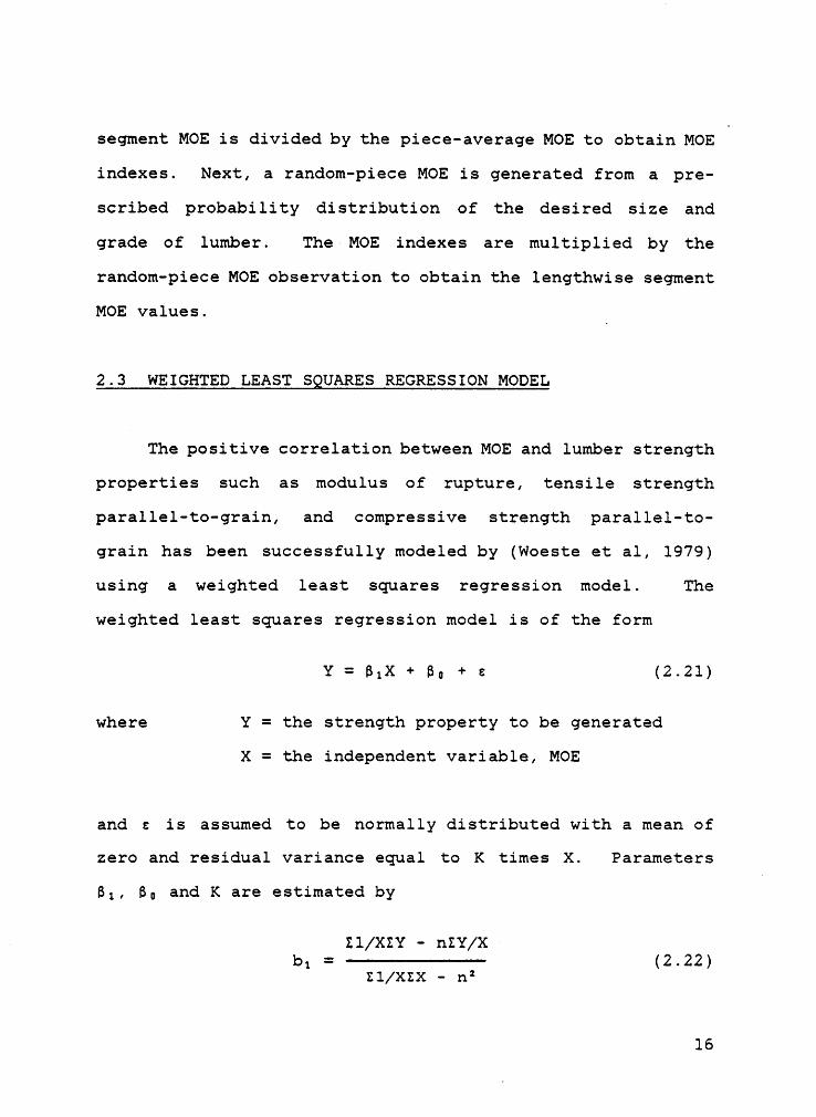
2.3 WEIGHTED LEAST SQUARES REGRESSION MODEL

The positive correlation between MOE and lumber strength

properties such as modulus of rupture, tensile strength

parallel·to-grain, and compressive strength parallel—to·

grain has been successfully modeled by (Woeste et al, 1979)

using a weighted least squares regression model. The

weighted least squares regression model is of the form

Y = BIX + B„ + s (2.21)

where Y = the strength property to be generated

X = the independent variable, MOE

and s is assumed to be normally distributed with a mean of

zero and residual variance equal to I< times X. Parameters

B1, Bu and K are estimated by

« Z1/XZY · nZY/Xb1 = ——--——-——-—- (2.22)

21/XZX — ¤=

16

. XzY/x - XYbg = ""***""'*'X21/X

· ¤ p

b„’sx“(1 - rz)K = ———————- (2.24)

Xrz

where r‘is the estimated linear correlation coefficient, sx:

is the estimated variance of X, and the summation over 1 to

n is implied.

In some cases, the weighted least squares regression

model, Equation 2.21, exhibits a lack of fit near the lower

left corner of the scattergram of strength versus stiffness.

Then, "it is highly probable that a logarithmic transforma-

tion on the dependent variable (strength. property) will

greatly improve the relationship" (Woeste et al, 1979). The

weighted least squares regression model becomes

= ßg + BIX +

€whereVar(E) = KX and the parameters B„, B1 and K are calcu-

lated by Equations 2.22, 2.23 and 2.24, respectively, by re-

placing Y with ln(Y).

17

CHAPTER III. EXPERIMENTAL DESIGN

3.1 DESCRIPTION OF MATERIAL -

One thousand pieces of l6—foot nominal 2-inch dimensionSouthern Pine lumber of two sizes and two grades were ob-

tained by competitive bid on the open market. Two sizes and

two grades were chosen so as to define the length effect for

a wide quality range to broaden the application of results.

The sizes and grades and the numbers of pieces of each were.

as follows:

Number Size Grade

250 2x4 No. 2 KDl5250 2x4 2250f—1.9E250 2xlO No. 2 KDl5250 2xlO 2250f-1.9E

The actual number of usable pieces varied slightly from the

above numbers. The No. 2 KD15 is a visual-stress grade de-

noted by VG and the 2250f—1.9E is machine stress—rated (MSR).lThe grades and sizes were chosen to cover the range of_

common truss spans found in practice.. A short span roof

truss would typically be designed with 2x4 lumber with the

lowest grade used being No. 2 KDl5 Southern Pine. For longer

spans, 2xlO machine stress—rated lumber would be common. The

grade 2250f-1.9E Southern Pine was chosen since it is the

highest grade likely to be used for roof truss construction.

18

In the Southern Pine structural lumber market, material

grade-stamped No. 2 most commonly includes material No. 2 and

better in quality, as was the case here. A quality supervi-

sor from the Northern Hardwood and Pine Manufacturing Asso-

ciation was contracted to visually regrade the No. 2 KDl5

material. The result of that regrade is tabulated below:

Number of Pieces2x4 2xlOSelect Structural Dense (SSD)‘ 35 31Select Structural (SS) 4 5No. 1 Dense 77 61No. 1 11 42No. 2 Dense 79 58No. 2 38 59Total 244 256

‘KD is dropped from the grade name for convenienceand is hereafter implied.

The "regraded" lumber was combined into four groups based on

similarities of allowable bending stress values, Fb, speci-

fied in the National Forest Products Association (1982) for

the individual grades. The grade or grades in each group,

the Fb values for the individual grades, and the numbers of

specimens resulting from the combinations are shown in Table _3.1, I3.1 CONDITIONING

The lumber was conditioned to equilibrium moisture con-

tent in a room controlled at 75°F and 68 percent relative

19

TABLE 3.1. The "regraded" No. 2 lumber groups, theirallowable bending stresses and the number of° specimens in each group.

-—-—---2X4·—---·— -—--—-—2XlO·-——-—-GROUP GRADE Fb NO. OF Fb NO. OF

I(psi) SPECIMENS (psi) SPECIMENS

11 SSD 2250 35 2200 31

2 SS 2150 81 1850 66No. 1 D 2150 1850

3 No. 1 1850 90 1600 101No. 2 D 1800 1650

4 No. 2 1550 39 1300 59

TOTAL 245 257

20

humidity (= 12% EMC). A capacitance moisture meter was used

to monitor the conditioning progress.l

3.1.2 ASSIGNMENT TO TREATMENT GROUPS

The lumber was assigned to the three test lengths such

that their distributions of strength would be as equivalent

as possible. A full-span modulus of elasticity (MOE) was

1 determined on all pieces by the vibration method. For the

MSR lumber, all pieces were ranked by MOE (2x4 and 2xlO in-

dependently). The five pieces having the lowest five MOE 1

values were randomly assigned to the 30-, 90- and 120-inch

test groups: one to the 30-inch groups and two each to the

90- and 120-inch groups. Only one was assigned to the

30-inch group because each 16-foot piece was long enough to

yield two specimens for the 30-inch test. The five pieces

with the next five lowest MOE values were randomly assigned,

and so on, until the three test groups were established with

approximately 100 specimens per test length.

The "regraded" visually graded lumber was ranked by MOE

separately for each "grade" group. They were then assigned

to the three test lengths in the same way as the MSR lumber.

Tables 3.2 and 3.3 list the assigned treatment groups and

number of specimens of the "regraded" visually graded lumber.

_21

TABLE 3.2. The number of specimens in each grade group andtreatment group of visually graded 2x4 are shown.

GROUP TREATMENT GROUP30—inch 90·inch 120—inch

1 14 14 14

2 34 32 323 36 36 36

14 14 16 16

‘ Totals 98 98 98

22

TABLE 3.3. The number of specimens in each grade group andtreatment group of visually graded 2x1O are shown.

GROUP TREATMENT GROUP30-inch 90·inch 120·inch

1 14 12 12

2 26 26 27

3 40 41 40

4 24 V 25 22 .

Totals 104 104 101

23

3.1.3 MEASUREMENT OF MOE

A flatwise static MOE was determined on four 30·inch

long segments in each specimen designated for the 30-inch

tension test, two on each side of the center line of thespecimens (Figure 3.1). Dead loads (a pre-load and a, finalload) were applied to the third-points of a 90-inch span withan air operated ram. The loads were 25 and 100 pounds forthe 2x4's and 75 and 275 pounds for the 2x10's. On severalspecimens with low stiffness, the system "bottomed out" andthe pre- and the final loads had to be reduced accordingly.

When testing the various segments, an upward force was ap-

plied on the opposite end at the center of the overhang tocounter the weight of the overhang and eliminate significant

reverse bending moments.

Deflections were measurmd (at pre-load and the final

load) between the load points with a LVDT mounted cu: a yokeand suspended from the specimen at the load points. Thistest arrangement permitted calculation of a shear-free MOE.

A rocker was provided at one support, at one end of thedeflection yoke to account for twist in some members. Aroller support at the end opposite the rocker support allowedfor the lengthing of the specimen as it was loaded. The de-

flection yoke was suspended from 1/4-inch dowels laying

crosswise on top of the specimen. The small diameter dowels

24

u u

QOIEO¤0¤•¢vc„¤-4G 4-J••-IVääoä-’S

O Q E·•Q•-Q· Gd! GO•—IH Q-H

· Q•,£HgfßäludlUU2 QSH -1-bu’QGUC'•¤•¤'¤GQQ-•••-•¤OQägJm'

M v HQ¤=J¢=1 cwvcsE-•¤ ¤J,:Q~e-•ääO22HQGWNQ GuQ2Q1 Usv:-•cs-•Q QQJHUB-'|QU3U_OscvcEco: 0 -QGUIU •HQQQ 20 3¢¤«1·M U-AHOJ ..:: Q_

0,.::44dlhnl-IO) "UU EUC2Q '¤-OQQQ) •G<JE: mmc:

' ¤¤•-·•Q3-•

Q ¤)22¤¤u2Q Qv: Qcco_ „c-'¤ .¤·•·-vuuobmv ccsv vm·•-•¤¤¤ -2EQIdle-42 UO03¢~1' 0M ¤•2<lJ0}H HH0u··¤q,eu„•:•vQc30O Q

Q GIUJ‘ OQ:cu*4-•••-OGMQJGIov--•: Ea:Q ·•-•uQHGJMU

5 3%·°$>«ä,-1 o0<<u.:¤»· •-JU: <¤E·•u

•—OO

MQ

Z,5

•—• coM ·«-·•E·• liloQ

. ZBJ

25

were flexible enough to "seat" on specimens rather than rock

on those that were cupped (convex side up).

Width and thickness were measured to the nearest 0.01

inch at the center of each 30-inch segment which were used

to calculate MOE for individual segments.

Three repetitions were performed on each segment and the

MOE values reported are the averages of the measurements.

3.1.4 TENSION TESTING »

In preparation for testing, the pieces designated for

the 30-inch length were cut in two pieces between

MOE—segments 2 and 3 and then trimmed on the opposite end to

a 90-inch length. The specimens designated for the 90-inch

and 120-inch tests were trimmed equally on both ends to total

lengths of 150 and 180 inches, respectively. Table 3.4 shows

the required arrangement of tensile specimens in the tensile

grips. Width and thickness were measured to the nearest 0.01

inch at the center of the test zone. Specimens were centered

between grips and loaded to failure in the U. S. Forest

Products Laboratory tension machine at a rate of 360 lbs/sec.

The specimens were tested in groups of 25, systemat-

ically varying the test length. This procedure permitted

testing 100 specimens without changing the machine settings,

e.g. 25 specimens each of 2x4 VG, 2xlO VG, 2x4 MSR and 2xlO

26

Table 3.4. Required arrangement of tensile specimens in thetensile grips.

Treatment Length between Length in Test SpecimenNo. Grips Grips Length

A 30 60 90*

B 90 120 150*

C 120 150 180

*Cut 2 from center of 16-foot piece*Cut from center of 16-foot piece

27

MSR for one length test, then switching to another length,

etc.

Defects associated with the failures were mapped and a

description of the failure recorded. The moisture content

and specific gravity were measured on a l·inch disc cut from' as near the failure as possible.

3.2 DATA ANALYSIS

_ The measured axial tensile force was used to calculatel

the tensile strength parallel—to—grain for each specimen.

Tables 3.5, 3.6 and 3.7 show the mean tensile strength for

each group of lumber. The mean tensile strength decreases

with an increase in length for every group from the 30·inch

specimen to the 90—inch specimen. Then, the mean tensile

strength either decreases or increases from the 90-inch to

120-inch specimen in the visually graded lumber. The mean

_ tensile strength continues to decrease from the 90-inch

specimen to the l20—inch specimen in the MSR lumber groups.

Figures 3.2 through 3.5 show the decrease in mean tensile

strength in every group from the 30·inch specimen to the

l20-inch specimen.

28

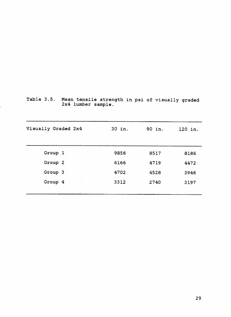
Table 3.5. Mean tensile strength in psi of visually graded· 2x4 lumber sample.

Visually Graded 2x4 30 in. 90 in. 120 in.

Group 1 9856 8517 8186Group 2 6166 4719 4472Group 3 4702 4528 3946

Group 4l

3312 2740 3197

V 29

Table 3.6. Mean tensile strength in psi of visually graded2x10 lumber sample.

Visually Graded 2x10 30 in. 90 in. 120 in. V

Group 1 9685 6572 6596

Group 2 5603 4268 4119Group 3 4644 4028 3412

Group 4 3035 2631 2084

30

Table 3.7. Mean tensile strength in psi of 2250f-1.9Elumber.

Size 30 in. 90 in. 120 in.

_ 2x4 9436 8107 8100

2x10 9270 8139 7976

31

Z}U')0. 10.0C)O .:1I 7.5 eI-LDZ ‘ _ .E|_ 5.0 ‘U')L1.!.1I" 2.5U')ZLu .I" IZ 0.0CE 0.0 30.0 60.0 90.0 120.0 2 150.0L; LENGTH (I NCHES) .

Figure 3.2 Mean tensile strength of the 2::4 2250f-l.9E MSR SouthernPine versus length of the test span. Tension specimens‘ were tested at 30-, 90- and 120-inch test spans. •

' 32

C.(D0. 10.0OO .Q .

_ UI 7.5I-(DZ _ . 1hä*__ 5.0U')

'

..1 F 11** 2.5(DZl.1J1-

' CE 0.0 30.0 60.0 90.0 °l20.0 150.0Li-L LENGTH (I NCHES)

Figure 3.3 Mean tensile strength of the 2::10 2250f-1.9E MSR SouthernPine versus length of the test span. Tension specimens

_ were tested at 30-, 90-inch and 120-:1.nch test spans.

33

2LD0. 10.0 ,1

Group 1 ·C)O

7.5|···[5 .Z Group 2 ''··-' .E s.oU.) Gr¤¤1¤3LU

Group 4JH205 lU')

ZL1J1-Z 0.0CE 0.0 30.0 60.0 90.0 120.0 150.0Li-‘ LENGTI-l (I NCHE.51

Figure 3.4 Mean tensile strength of the 2x4 No. 2 KDl5 Southern Pineversus length of the test span. Tension specimens were ·tested at 30-, 90- and 120—inch test spans.

34

3_ U10. 10.0 ‘Group 1 “

· .

O5I 7.5I-L'). ‘ZI.1J Group 2CP s.0 ‘I" Group 3

L1J..1 Group 4

LOZL1.1I··Z 0.0 I ‘CE 0.0 30.0 60.0 90.0 120.0 150.0Lg LENGTH (INCHE'5)

Figure 3.5 Mean tensile strength of the 2x10 No. 2 {GHS Southern Pineversus length of the test span. Tension specimens weretested at 30-, 90- and 120-inch test spans. —

35

Tables 3.8, 3.9 and 3.10 list the coefficients of vari- _3

ation, COV, of the tensile strength. The COV generally in-.creases with a decrease in grade quality. The only exception

is an increase in COV from Group 3 to Group 4 in the 120-inch

specimen of 2xl0 visually graded lumber.

_ Next, the fifth percentile tensile strength was calcu-

lated for each group of lumber. A lognormal distribution was

assumed and a fifth percentile value was calculated from the

distribution fit. Again, a decrease in tensile strength with

an increase in specimen length can be observed (Figures 3.6

- 3.9).

The correlation structure of the tensile strength was

considered along the piece of lumber. Since two 30—inch

segments were taken from a single piece of lumber, the cor-

relation coefficient between segments "l" and "4" was deter-

mined for each specimen of the 30-inch treatment group. The

likelihood that the tensile strength is correlated between.

segments "l" and '%U' was tested using the t distribution

(Haan, 1977). The hypothesis H„ = pl,4 = 0 was tested, pl,4being the population correlation coefficient of the tensile

strength between segments "l" and "4" of the 30—inch speci-

mens. If p = 0, then the quantity

t = r[(¤—2)/(1-r')1% (3 1)

r = sample estimate populationcorrelation coefficient

36

Table 3.8. Coefficieht of Variation of the tensile stengthin Visually graded 2x4 lumber sample.

Visually Graded 2x4 30 ih. 90 in. 120 ih.

Group 1 0.250 0.215 0.270

Group 2 0.285 . 0.364 0.310

Group 3 0.428 0.405 0.506

Group 4 0.430 0.452 0.541

37

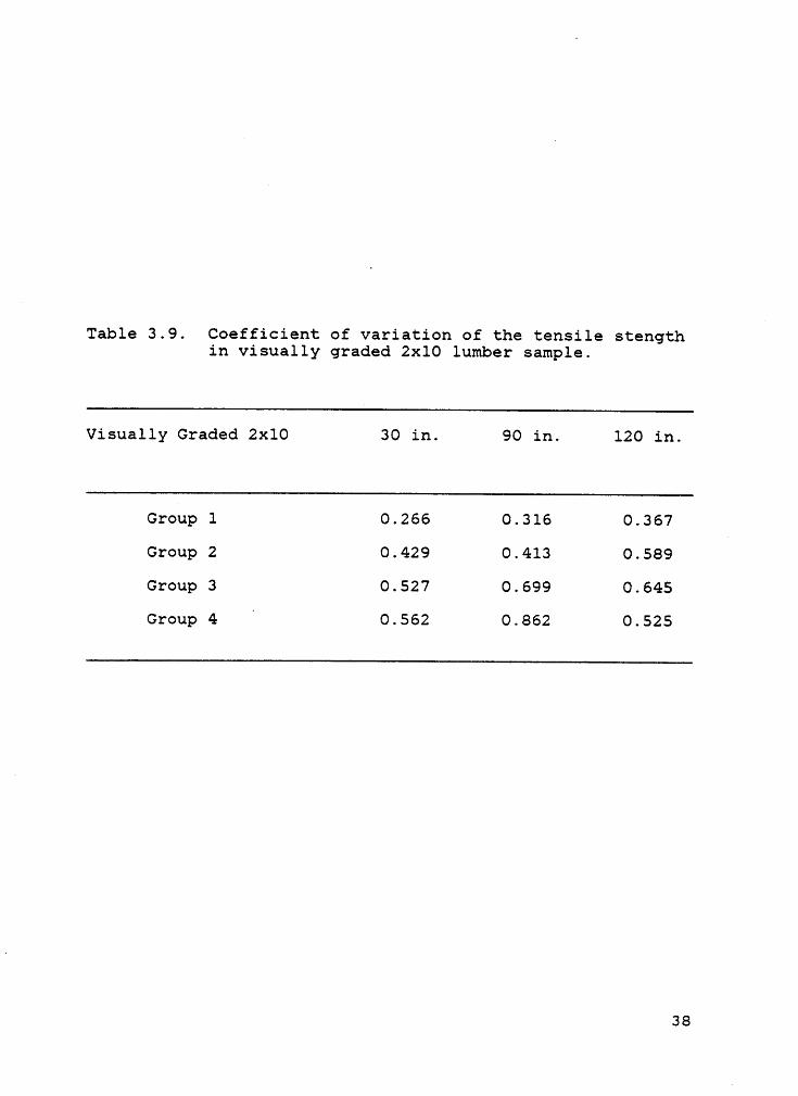
Table 3.9. Coefficient of variatiom of the teusile stengthin visually graded 2x10 lumber sample.

Visually Graded 2x10 30 ih. 90 in. 120 in.

Group 1 0.266 0.316 0.367Group 2 0.429 0.413 0.589

Group 3 0.527 0.699 0.645Group 4

n0.562 0.862 0.525

38

Table 3.10. Coefficient of Variation of the tensilestrength of the 2250f—1.9E lumber.

Size 30 in. 90 in. 120 in.

2x4 0.305 0.286 0.2892x10 0.251 0.252 0.262

39 ·

I3U')0.O -;• 10.0:[ „I-LDZ

-

4Lu.!JpaLD 1ZL1.1

- "" 2.sL¤J.J .paI-Z

0.0 30.0 60.0 90.0 120.0 I 150.0_ C: LENGTH (I NCHE5)

L1.!0. .II-LD

Figure 3.6 5th percentile tensile strength of the Zxé 2250f-l.9E MSR .Southern Pine versus length of the test span. Tension

. specimens were tested at 30-, 90- and lZ0—inch test spans.

I 49

C.0.G .C)

10.0 I ”

II- .

~|_,_| 7.5Q 7P eU') 7Ln.!JZ

LnJI" 2.sL1J..1"I .I'-Z ·o.00.0 30.0 60.0 r 90.0 120.0 150.0Q LENGTH (INCHE5)Lv.|O.II-U')

Figure 3.7 Sth percentile tensile strength of the 2::10 2250f-l.9E MSRSouthern Pine versus length of the test span. Tensionspecimens were tested at 30-, 90- and 120-inch test spans.

· 41

C.U')0.OO

10.0I .I-(DZ

}. .(D Gmup1‘L1.]_-J S•°•-•U)2: Group 2L•..I" 2.s _

Group 3L1J-1 Gr¤¤p4"" .

. I-Z 0.0LLBJ 0.0 30.0 60.0 I 90.0 120.0 150.00: LENGTH (I NCHE5)LL] .CLII-LD

Figure 3.8 Sth percentile tensile strength of the 2x4 No. 2 KDl5Southern Pine versus length of the test span. Tensionspecimens were tested at 30-, 90- and 120-inch test spans.

’ 420

,2,LD0- .OOtä 10.0

I|·—G .Z .|_,_| 7.5OZI-(*0 Group 1LLJ—-I

-

ZL|JE 2-5 Group 2LIJ Group3iGroup1-

.Z 0.0LIJ 0.0 30.0 60.0 p 90.0 120.0 150.0LENGTH (I NCHE5)

LnJQ_ .II-LD

Figure 3.9 Sth percentile tensile strength of the 21:10 No. 2 @15Southern Pine versus length of the test span. Tension' specimens were tested at 30-, 90- and 120-inch test spans.

Gg 43

has a t distribution with n—2 degrees of freedom where n is

the sample size. To test the hypothesis Ho: pll4 = 0, the

test statistic was calculated from equation 3.1 and H„ was

rejected when [tl The percentile value,

tl_a/2In_2 was chosen at the 0.05 level of significance.Table 3.11 shows the sample estimate correlation coef-

ficient rll4 and the result of the hypothesis test for each—grade and size. The hypothesis that the tensile strength in

segments "1" and "4" are not correlated was rejected for both

the 2x4 and 2xl0 2250f-1.9E lumber. The hypothesis was also

rejected for Groups 2 and 3 of the 2x4 lumber, Group 3 of the

2xlO lumber and for both the 2x4 and 2x10 grade—stamped No.

2 lumber.

44

Table 3.11. Summary of hypothesis test illustrating theV correlation of the ultimate tensile stress in

segments "1" and "4" of the 30-inch groups atthe 0.05 significance level.

Size Grade Group rl’4 H„: pl’4 = 0

2x4 2250f-1.9E 0.444 reject

2x4 Group 1 0.380 cannot reject

2x4 Group 2 0.827 reject

2x4 Group 3 0.776 reject

2x4 Group 4 0.649 cannot reject

2x10 2250f-1.9E 0.402 reject

2x10 Group 1 -0.120 cannot reject

2x10 Group 2 0.299 cannot reject

2x10 Group 3 0.555 reject

2x10 Group 4 -0.096 cannot reject

2x4 No. 2 KD15 0.831 reject‘ "as graded" ·

2x10 No. 2 KD15 0.589 reject"as graded"

45

CHAPTER IV. MODEL DEVELOPMENT

The purpose of this study was to develop a length effect

model for tensile strength parallel-to-grain. The data from

the 30-inch treatment groups were used to derive the parame-

ters for the model. Because the number of specimens in each

treatment group of visually graded lumber was small, it was

decided, for purposes of demonstrating the method of model-

ling, to recombine the re-graded groups. In order to deter-

mine the success of the model, probability distributions of

tensile strength were simulated for a 90-inch length and a

120-inch length and then independently verified against the

test data from the 90-inch and 120-inch treatmentgroups.The

first approach used to derive the probability dis-

tributions of tensile strength parallel-to-grain was to use

Weibull's "weakest-link theory" (1939). Using Weibull's

theory, the lengthwise segments of a lumber specimen are as-

sumed to be non-correlated. The second model developed takes

into account the possible lengthwise correlations of tensile

strength. .A detailed description of each model is included

in the following sections of this chapter.

46

4.1 DEVELOPMENT OF A MODEL ASSUMING INDEPENDENT SEGMENTS

Using Weibul1's "weakest-link theory" (1939), the ulti-

mate tensile strength in a 120-inch specimen of lumber can

be defined as the tensile strength in the weakest 30-inch

segment of the four 30-inch segments forming the specimen.

Likewise, the tensile strength in the weakest segment of the

three 30-inch segments forming a 90-inch specimen is the

tensile strength of that specimen. According to Ang and Tang

(1984), if the segments forming a specimen of n segments are

assumed to be statistically independent and identically dis-' tributed, the CDF of the tensile strength of a specimen with

n segments, is

_ _ _ nFY1(Y)—l ll FX(Y)1 (4.1)

It follows that the probability density function (PDF) be-

comes

f (Y) = ¤[l — F (Y)1“°lf (Y) (4 2)Y, X X '

where: y = tensile strength parallel-to-grain

n = number of 30-inch segments

fX(y) = PDF of tensile strength of a30-inch segment

FX(y) = CDF of tensile strength of ay 30-inch segment

47

The first step in the development of the model was to

determine the PDF's and CDF's for each of the 30-inch treat-_

ment groups. Figures 4.1 through 4.4 show histograms of

tensile strength parallel-to-grain from each of the 30-inch

treatment groups. A visual inspection of Figures 4.1 through

4.4 suggested that the lognormal distribution might provide

a good fit. Accordingly, the lognormal distribution was

overlayed on the tensile strength histograms shown in Figures

4.1 through 4.4. Visual inspection of the distribution in-

dicated a good fit.

A weakest—link model was formed using Equation 4.2. So,

fY1(y) equals the distribution of the 90-inch or 120-inch

data, assuming the segments are independent; n equal 3 for

the 90-inch data and n equal 4 for the l20—inch data; and

fX(y) and FX(y) are the lognormal distribution for the

30-inch data and its probability distribution, respectively.

Figures 4.5 through 4.8 show relative frequency histograms

of the tensile strength of 90-inch treatment groups. Super-

imposed onto the histograms are the appropriate probability

functions, fY1(y), with n equal 3. Figures 4.9 through 4.12

show relative frequency histograms of the tensile strength

120-inch treatment groups and fYI(y) with n equal 4 superim—

posed onto the histograms.

Q 48

•-• ° uI

.I ><°?CON · 100 Lognormal Parameters

X .1, -· 9.11 ·Ei ‘

E -· 0.304N_

-uf? ·Dv-•CU· l.I.I0:U- .9cn I

O”

·II0

5 10 15 20 _

'1'ensile Strength (1000 psi)

Figure 4.1 A lognormal distribution is superimposed on the histogramof the tensile strength of the 2::4 22S0f·1.9E MSR 30"treatment group.

49

FKBE · „ . .V ·· .- :_ ’· . .Q .«« N = 100 Lognormal_Parameters

>< 1 A - 9.100*1 W<‘¤L c =· 0.275

E? .VCZ!

LL] I“ ÄL1- O. V F„ ’ I ‘

Ä(F\D _ I | I I

· O 5 10 15 20 ·A Tensile Strength (1000 psi)

Figure 4.2 A lognormal distribution is superimposed on the histogramof the tensile strength of the 2xl0 2250f-1.9E MSR 30"treatment group.

50

0-0

I

gg ._ V

CJ ,, '___' N 98 Lognormal Parameters

X ‘ 1 - 8.54gg c =- 0.490

>—

ä¤.«.1"! .DINGL1.IC1:"‘ 1

Ü05 10 15 20Tensile Strength (1000 psi)

I

Figure 4.3 A lognormal distribution is superimposed on the histogramof the tensile strength of the 21:4 No. 2 KD15 30"treatment group.

51

1-•|

1 .IIBE

·‘

'¤' .Ü N = 104 Lognormal Parameters•-O

Ä = ,X ‘ 839Qc · 0.586m

>-Q

.L) 1Z .GJ 1LJ.!OS1.1.„

1 I I·¤¤...._„„0 5 10 ' 15

20.

Tensile Strength (1000 psi)

Figure 4.4 A lognormal distribution is superimposed on the histogram‘

of the tensile strength of the 2xlO No. 2 KDl5 30"treatment group.

S2

alsl

ZO7

>-1 äM 1.8

‘

Z: .¤ 1Lu“ 1'·‘· 0.6„ „ ul. Lu--°0.0 11.0 8.0 · 12.0 18.0UL T I MHTE TENS I 0N (1000 P5 I )

Figure 4.5 The histogram of the ultimate tension of the 2::4 2250f-1.9EMSR 90" treatment group is shown. The probabilitydistribution, fY (y), with n=•3 is superimposed onto thehistogram. 1

sa

>—L.!ZLU 1.63cs 1L¤.IC: .'·‘· 0.8

'LL

0.0 11.0 _ 8.0 12.0 18.0UL T I MQTE TEN5 I ON GOOO P5 I 1

Figure 4.6 The histogram of the ultimate tension of the 2xlO 2250f·l.9EMSR 90" treatment group is shovm. The probabilitydistribution, fY , with n•3 is superposed onto the

W histogram. 1

‘ 54

ÜI.0 ‘

3.0l \

>-°2’LU 2.0:G 1äé'·‘· 1.0M

I hl!.¤0.0*-1.0 8.0 12.0 16.0ULTIMGQTE TENSION QOOCJ PSI)

Figure 4.7 The histogram of the ultimate tension of the 2x4 No. Z KDl590" treatment group is shown. The probability distribution,EY , with n•3 is superimposed onto the histogram._ l

55

4.11

A 3I3

>'ELu 2.2D .C5I-IJ.Q:L'* 1.1 ‘

0.0 1-1.0 8.0 12.0 18.0UL T I MQTE TENS I ON (1000 PS I)

Figure 4.8 _The histogram of the ultimate tension of the 2xlO No. 2 KD1590" treatment group is shown. The probability distribution,fY , with :1-3 is superimrosed onto the histogram.1

56

alsI

2l7

>·

1.8DGLv.!O!'·'· 0.8

„„ |1||*·I.0 8.0 12.0 16.0

ULTIMHTE TENSION (1000 PSI)

. Figure 4.9 The histogram of' the ultimate tension of the 21:4 2250f·l.9E120" treatment group is shown. The probabilitydistribution, EY , with n=4 is superimposed onto thehistogram. 1

57 ,

3.0

>-(2,1Lu 2. 0

D .GL1J0:"· 1.0 I” 0.0 •·I.0 8.0 ’ 12.0 16.0

ULTIMPTE TENSION 11000 PSI)

Figure 4.1.0 The histogram of the ultimate tension of the 2xlO”22S0f·l.9E l20" treatment group is shown. Theprobability distribution, EY , with n•4 is superposedonto the histogram. 1

S8

3.6

>-U 1ZLL} 2. llIJ 1

. Q ’

L1.!Q:'·'· 1.2 ‘I Ähll -0.0 ’ 1

0.0 11.0 8.0 12.0 16.0UL T·I MFITE TENS I 0N (1000 PS I1

' Figure 4.11 The histogram of the ultimate tension of the 2x4 No. 2ICDIS 120" treatment group is shown. The probabilitydistribution, fY , with n=-4 is superimposed onto thehistogram.

1S9

SIZ

30g

>-‘2’LU 2. 6DGL1.1 F °¤= 1LI-

Ä l~I0.0 *4.0 8.0 2 12.0 18.0

ULTIMFITE TENSION (1000 PSI)

Figure 4.12 The histogram of the ultimate tension of the 2xlO No. 2@15 120" treatment group is shown. The probabilitydistribution, fY , with n=4 is superimposed onto thehistogram. 1

60

4.2 DEVELOPMENT OF A MODEL OF CORRELATED SEGMENTS

Table 3.11 shows that there is a significant correlation °

between the tensile strength of the first and fourth 30-inch

segments in each of the four grade and size groups. There-

fore, it is reasonable to assume that lumber exhibits lag-1

serial correlation; ie, that the tensile strength parallel-

to-grain is correlated to the tensile strength of the previ-A

ous segment. A tensile strength - length effect model was

developed taking into account the serial correlation of

tensile strength between segments. In the discussion that

follows, the method used to develop the model will be de-

scribed. This method involves the following steps.

1.) Determine 30-inch segment MOE's for a lumber ‘specimen using a MOE variability model (Kline etal, 1985).

2.) Input segment MOE's into an appropriate weightedleast squares regression model to obtain tensilestrength parallel—to-grain for each of the30-inch segments of the lumber specimen.

3.) Using a weakest-link theory, the minimum segmenttensile strength is defined as the tensilestrength of the lumber specimen.

4.2.1 GENERATION OF SEGMENT MOE'S

A MOE variability model (Kline et al, 1985) generated

serially correlated MOE's along 30-inch segments for a piece

61

of lumber. The type of lumber, number of segments and a

random observation from a distributon of average MOE values

were inputted into the model to obtain the segment MOE's.

In order to eliminate the generation of unrealistic

segment MOE values, the MOE variability model (Kline et al,

1985) was modified. A minimum segment MOE, EMIN, and a max-imum segment MOE, EMAX, were inputted into the model. If a

generated segment MOE was not in the specified range as in-

dicated above, another series of segment MOE’s was generated

in its place. The minimum and maximum segment MOE’s selected _

‘ for the modified MOE variability model were the minimum and

maximum segment MOE’s from the four data sets of 2X4 and 2X1O

2250f-1.9E and NO.2 KD15 Southern Pine used in the develop-

ment of the MOE variability model (Kline et al, 1985). Table

4.1 lists the minimum and maximum segment MOE values used in

the modified MOE variability models. Appendix A contains a

program listing of the modified model.

The distributions of MOE to be inputted into the four

MOE variability models were determined by using MOE data from

the 30-inch treatment groups. A lognormal distribution was

fitted to the 30-inch MOE values for both groups of MSR lum-

ber. Figures 4.13 and 4.14 show the histograms and the fit-

ted lognormal density curves. A 3—parameter Weibull

distribution was fitted to the VG 30-inch lumber groups.E Figures 4.15 and 4.16 show the histograms and the fitted

lognormal density curves. The fitted density curves and

62

TABLE 4.1. The minimum and maximum 30—inch segment MOEvalues for each grade and size group used in thedevelopment of the MOE variability model (Klineet al, 1985).

SIZE GRADE EMIN EMAX(x

10‘psi) (x 10° psi)

2x4 2250f—l.9E 1.579 3.623

2x4 Grade-stamped 0.461 3.245No. 2

2x10 2250f-1.9E 1.679 3.630

2x10 Grade-stamped 0.528 3.236No. 2 ·

63

N = 50 Lognormal Parameters‘ A = 14.75N..1 C =· 0.133

~

E. DG [L1.! · .tc [ [LL [ |v

O

1Q lll Il!@0 1 .0 2.0 3 .0 4 .0

1

MOE (million psi) _

Figure 4.13 30-inch segment MOE values measured from the 2x42250f-1.9E MSR 30" treatment group were used to formthe histogram. A lognormal distribution fit issuperimposed onto the histogram.

· 64

*9 .”

N =- 50 Lognormal Parameters _

A = 14.68I... 1; =· 0.135 }

>-E. LUG]DOÜL1.I0CLI.

-

O

Q I‘ @0 I .0 2 .0 3 .0 4 .0Mou <m1111¤¤ ps1>

Figure 4.14 30-inch segment MOE values measured from the 2xlO· 22SOf-1.9E MSR 30" treatment group were used to form

the histogram. A lognormal distribution fit issuperimposed onto the histogram.

65

og .° · N • 49 Weibull Parameters11 · 0.522 IG? 1 378 ·Q o . I

- T1 • 2.689>__-

.

äDO

.°‘ VL1.9 1 I¤ I I . I.@0

1 .0 2 .0 3 .0 4 .0

· MOE (million psi)

Figure 4.15 30·inch segment MOE values measured from the 2x4 No. 2KDl5 30" treatment group were used to form thehistogram. A 3-parameter Weibull distribution fit issuperimposed onto the histogram.

66

·—• .. 1$2

D

N =• 52 I Weibull ParametersX u · 0.345

D(5 0 = 1.604

n · 2.688>-äuf?DV. _ _

G· LL1O1LL. • '

9

‘ Q I |@.0 1.0 2.0 2 .0 4.0 _

MOE (million psi)

Figure 4.16 30·inch segment MOE values measured from the 2xlO No. 2KDIS 30" treatment group were used to form the histogram.A 3-parameter Weibull distribution fit is superimposedonto the histogram.

67

histograms were visually inspected for conformance of the

lapplied fit to the data. Visual inspection of the distrib-

utions indicated a good fit.

Limits were assigned to prevent the generation of unre-

alistic piece-average MOE values. A minimum average MOE,

ECMIN, and a maximum average MOE, ECMAX, were inputted intothe tensile strength - length effect model. If a MOE value

was generated which exceeded these limits a new value was

generated„ This procedure results in selecting random ob-

servations of average MOE values from a truncated distrib-

ution. The truncation points selected for the models were,

ECMIN = EMIN + O.3xlO‘ psi (4.3)

and EOMAX = EMAX - O.3xlO‘ psi (4.4)

where EMIN and EMAX are listed in Table 4.1 for each grade

and size group. _

4.2.2 WEIGHTED LEAST SQUARES REGRESSION

A weighted least squares regression model developed by

(Woeste et al, 1979) was used to generate tensile strength

values parallel-to-grain for the 30-inch segments of a lumber

specimen when the MOE of the segments was given. Equation

2.21 was used with Y, the dependent variable equal to tensile

strength parallel-to-grain. The estimated parameters b„, bl

68

and l< were calculated for each of the grade and size groups

using the MOE and tensile strength data from the 30-inch

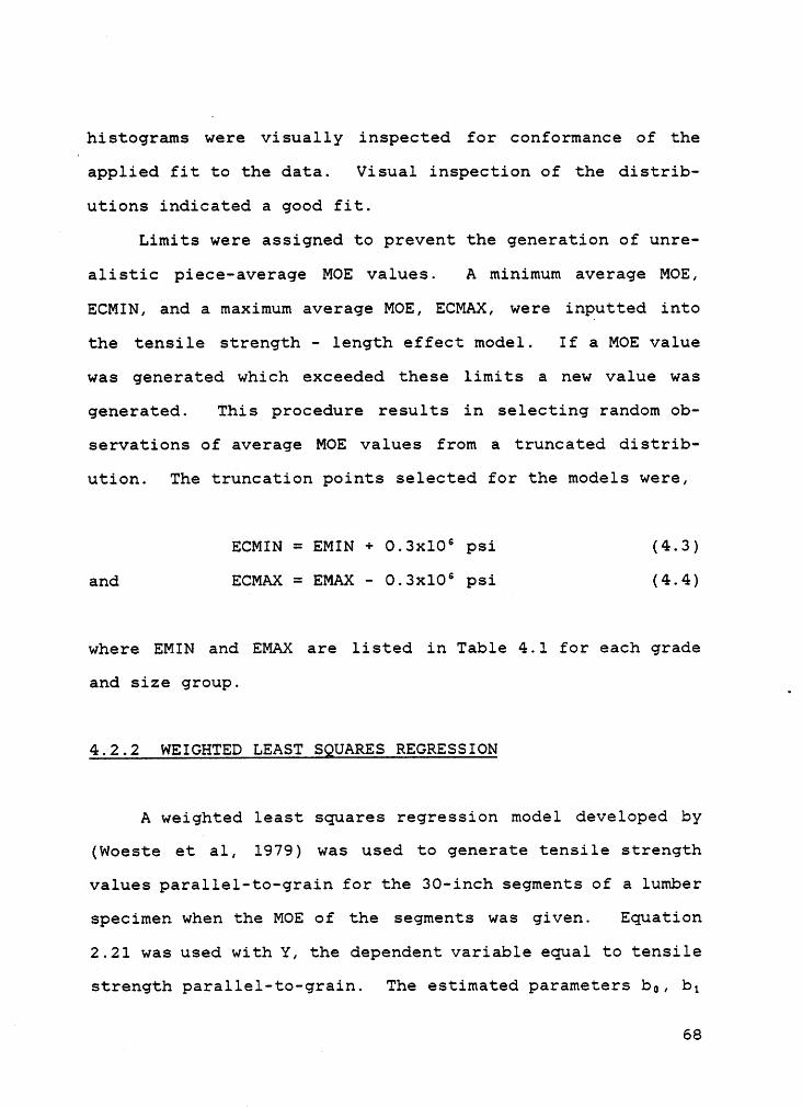
treatment groups. Figures 4.17 through 4.20 show

scattergrams of the actual MOE-tensile strength pairs with

overlays of the regression lines and curves which bound 99

percent of the residuals under the assumptions of the model.

The data points should lie symmetrically about the regression

line if the correct model is used. However, each of the four

groups exhibits a lack of fit near the bottom 99 percent

boundaries. Also, the MSR ZX4, VSR ZX4 and VSR 2Xl0 groups

exhibit a lack of fit since data points exceed the upper

boundary.

Woeste et al (1979) found that when data exhibit this

type of lack of fit, it is likely that a logarithmic trans-

formation on the dependent variable, tensile strength in this

icase, will greatly improve the relationship. Hence, the new

regression model is given by Equation 2.25.

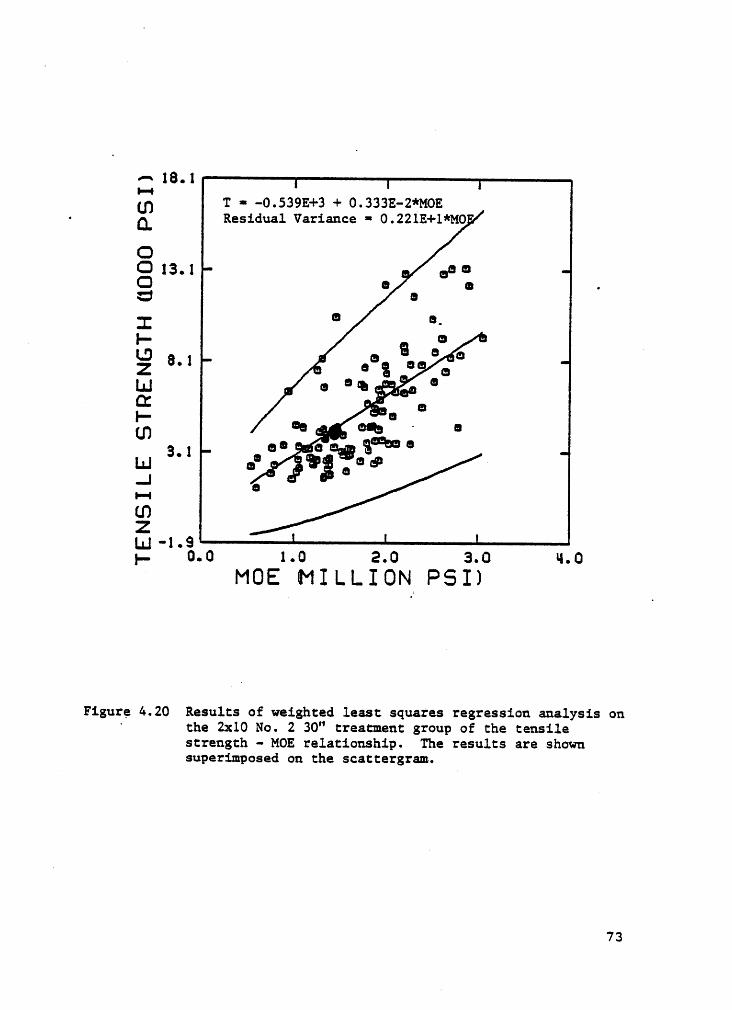
Figures 4.21 through 4.24 show plots of the transformed

regression lines along with the 99 percent boundaries over-

layed on scattergrams of the actual data. These models dis-

played no obvious lack of fit and, therefore, were used to

simulate subsequent tensile strength values. These models

are also practical since they are unlikely to simulate values

of near zero strength, a characteristic that is assumed to

be rare.

69

^ 2*4.09 I

•—• 1: · O.459E+3_+ 0.3531:-z*M0~,;Residual Variance ¤ 0.233E+1#MOE

CJO 18.0 ,3¤ ¤

l¤ •E ‘ °. 8 8.

Q 12.0 3*9Lu B Q l

6E ·”889an — 8* „_g„g‘=°¤°

6.0 G $1: 8 „L1,] ¤ o QQ B

_ |-lU') · .ZP OO 0 1 O

OMOEMI LLION PSI)

Figure 4.17 Results of weighted least squares regression analysis onthe 2::4 2250f-1.9E 30" treatment group of the tensilestrength - MOE relationship. The results are shownsuperimposed on the scattergram. °

vo

A 2*|.0•-•U-) T = O.427E+4 + O.2lOE—2*MOE0- Residual Variance = 0.245E+1*MOEO 0O 18.0O .SI ‘ ¤

GQQB g

LU Ga & ÜB G g GE °4 E ·%°—**°“ °6 6 0 °!’ ¤°‘§° °Ln.! ° •° ° °-| ¤

LDZ|- 0. 0 1 . 0 2. 0 3. 0 *-1. 0

MOE MILLION PSI)

Figure 4.18 Results of weighted least squares regression analysis onthe 21:10 2250f—l.9E 30" treatment group of the tensilestrength · MOE relationship. The results are shownsuperimposed on the scattergram.

» 7l

^ 18.1 _I-ILD *1* · -0.72412;+3 + 0.379E-2*MoE0- Residual Variance • O.l66E1*M0O3 13.1 ° L5 · o:1: L .° ° °1- aa ¤ °b “ ’*5 8.1 °

•=* ¤¤ °El ¤ zu o

a QI,. 0 Q B * .an J dg!3.1 °’ I..1J ¤ a am ·...I1-•

. LDZO 31. 0.0 1.0 2.0 3.0 •-1.0

MOE MILLION PSI)

Figure 4.19 Results of weighted least squares regression analysis onthe 2x4 No. 2 30" treatment group of the tensilestrength — MOE relationship. The results are shownSup€1°iIIlpOS€d OD. the SCBCCEIQYSIII.

72

A 18.1Z; T · -0.539E+3 + O.333E—2#MOE

· Q- Residual Variance =· O.22lE+l*MO

S 13. 1 aß ¤CD 0 0 .c 0:1: ° °~. I- °Ü 8 1 B g lZ ° ° S “ “ 0L¤J 0 ‘ Q °7 Gr- Ba ¤ °m0¤ 0 3 °.I 0•-1LDZy- 0.0 1.0 2.0 3.0 *-1.0

MOE (MI LLION PSI)

Figure 4.20 Results of weighted least squares regression analysis on° the 2xlO No. 2 30" treatment group of the tensilestrength - MOE relationship. The results are shownsuperimposed on the scattergram.

73

·___ 1¤(‘1‘) - 8.14 + 0.381E—6*MOEF., Residual Variance • 0.258E-7*MOE

2·

9•8 QII-- o B ggg, GLQ U Ü GZ Q BI Lu 9 2 I Q $9 8 o Q

°G ° Q °o amI- Q ° a aaa °LD „ a °¤ PMJ_, Q 0 GH 8.6 Q „

·ZMJI:Z 8.0__; 0.0 Q 1-0 2.0 3.0 ¤1.0

MOE IMILLION PSI)

_ Figure 4.21 A weighted least squares regression model was used on thetransformed data of the 2x4 2250f—1.9E 30" treatmentgroup and is graphically illustrated with the scattergram.

74

lolql

ln(T) =- 8.48 + 0.259E-6*MOE:3 Residual Variance =· O.334E—7*MOELDQ: 9. 8II- ä 8L-D aß a2 ¤Lg 9 2 a ¤ gb Q L ·G ° Q ga Q cäI" , Q 0LD MB 9¤°.LU n Bag naja a

9 ..l an “

ZLIJ aZ 8. 0_; 0. 0 I . 0 2. 0 3. 0 Il. 0

MOE IMILLION PSI)

Figure 4.22 A weighted least squares regression model was used on thetransformed data of the 2xlO 2250f-1.9E 30" treatmentgroup and is graphically illustrated with the scattergram.

75

um · 7.27 + 0.744E-6*MOE:3 Residual Variance ¤ 0.629E-7*MO

22I·II-10 ° 1 I

• a°

-. —·_. Qgf s.o ° ¤° . 66 ¤1- 1 F ° : °LD ¤ °¤ _

LU¤*°__'B -.7 B B8. 0 o ¤ ¤I-I2 ° “L1.1 ° _ ¤C_ Z 7.0

MOE MILLION PSI)

Figure 4.231 A weighted least squares regression model was used on thetransformed data of the Zxh No. 2 30" treatment group andis graphically illustrated with the scattergram.

76

10.8_ 1¤<'r> · 7.16 + 0.717E-6*MOE'_'» Residual Varian<:e•0.93OE—·7* MOE(D

· I- E o mLD ¤~°° :°°o° QZ Q B Ü

8.*1 BB Q G.° jg · é

LIJ QB—‘

7 2 °C(.0ZLLJCZ 8.0 1_; 0.0 1.0 2.0 3.0 (1.0

MOE (MILLION PSI)

Figure 4.24 A weighted least squares regression model was used on thetransformed data of the 2xlO No. 2 30" treatment group andis graphically illustrated with the scattergram.

77

4.2.3 SPECIMEN TENSILE STRENGTH

The final step was to generate values of tensile

strength for each of the 30-inch segments of a lumber speci-

men. Using a weakest-link theory analagous to Weibull's

"weakest-link theory" (1939), the minimum 30-inch segment

tensile strength is the tensile strength of the lumber spec-

imen.V

It was felt that a.maximum tensile strength value should

be inputted into the model to prevent the generation of un-

realistic tensile strength values of the lumber specimen.

For this study, the maximum tensile strength of the 30-inch

segments of the four data sets of 2X4 and 2XlO NO.2 KDl5 and

2250f-1.9E MSR Southern Pine, 17737.0 psi, was chosen as the

best estimate of the maximum tensile strength. If a specimen

tensile strength value greater than 17737.0 psi was gener-

ated, the generation procedure would generate a new set of

segment tensile strength values. Thus, a new tensile

strength value of the lumber specimen was determined. As

stated before, the maximum tensile strength value for this

study was selected from the available test data. However,

users of the model can input their own. maximum tensile

strength value.

78

4.3 PRELIMINARY VALIDATION RESULTS

Since the tensile strength — length effect models wereU

developed using the data from the 30-inch treatment groups,

the models were independently verified against the test data

from the 90—inch and l20—inch treatment groups. Both models

described in sections 4.1 and 4.2 failed to predict the ac-

tual tensile behavior of the 90-inch and 120-inch treatment

groups. However,the correlated segment model of section 4.2

provided a better fit than the independent segments model,

which suggested that perhaps the correlated segment model

could be refined to successfully model the tensile strength

behavior in a lumber specimen.

n4.3.1 INDEPENDENT SEGMENTS MODEL

A visual appraisal of Figures 4.5 through 4.12 suggests

that the tensile strength - length effect model which assumes

non·correlated segments underpredicts the tensile strength

of a lumber specimen. In addition to the visual test, a

Kolmogorov-Smirnov goodness of fit test was conducted for

each of the eight models. All of the models were rejected

at the 5 percent significance level. This result is not ·

counter·intuitive since Table 3.11 shows that there is a

significant correlation. between segments 1 and 4 i11 the

79

30-inch treatment groups, which indicates that there ;is a

significant correlation between the 30-inch segments.

4.3.2 CORRELATED SEGMENTS MODEL

Tensile strength ·· length effect models were developed

for ZX4 visually graded and MSR 90-inch and 120-inch pieces

of lumber using the procedure which assumes the segments are

correlated. Two-thousand average MOE values were generated

and inputted into the modified MOE variability model for each

of the four groups. The segment MOE values were then used

in the weighted least squares regression to obtain the

tensile strength parallel-to-grain for each 30-inch segment.

The tensile strength values of the generated lumber specimens

were then determined using a weakest-link theory.

Next, the PDF's for each of the tensile strength models

were determined in order to compare them to the actual test

data. A visual inspection indicated that the lognormal dis-

tribution best fit the generated tensile strength values of

each model. Figures 4.25 through 4.28 show relative fre- .

quency histograms of the tensile strength of the 90-inch and

l20-inch treatment groups of'both the ZX4 visually graded and

MSR lumber. The appropriate correlated segment models are

superimposed onto the histograms. Also, visual inspection

indicated that the models do not adeguately describe the

data. The four models were rejected using a Kolmogorov-

80

_ >·LJZ .LL] 1.6DGLI.!O:L'- 0.8

.

'

Y0.0 *1.0 8.0 12.0 16.0

- ULTIMPTE TENSION (1000 PSI)

L'Figure 4.25 The histogram of the ultimate tension of the 2x4

2250f-1.9E 90" treatment group is shown with thecorrelated segment model probability curvesuperimposed onto the histogram.

81

„ 30 6

20 7

_ >-1..)Z|_,_| 1. 83GL1.)Q:L'- 0. s

, !|„„0.0 1-1.0 8.0 12.0 16.0 ·ULT IMPTE TENSION (1000 PSI)

Figure 4.26 The histogram of the ultimate tension of the 2x422SOf·l.9E l20" treatment group is shown with thecorrelated segment model probability curvesuperimposed onto the histogram.

82

Q 6.6 ·

Z Q = ä( . Q 2 ‘

. u_|1.8 Q. . Q ~ Q„ : Ä Ä

G T‘i_‘·‘- 0.6j°g_gQ •.|,0· n 8.0- 12.0 16.0UL T I MFITE TENSI 0N (1000 P5 I)

Figure ¢.27 '1.'he;histogram .of· the ultimate tension oftheÄ2x4No.2 90" treatment group is shown with the correlated

segment model probability curve superimposed ontothe histogram. _ . Q

. Q . . 83

als

2.7

Q „[JJ 1.8

‘

Z1¤ Ä|.¤J=== V‘é‘·0.6 Ä I Ü'UL T I MQTE TENS I 0N (1000 PSI)

Üigure 4.28 The histogram of the ultimate tension of the 2x4 No. 2l20" treatment group is shown with the correlatedsegment model probability curve superimposed onto thehistogram.

84

Smirnov goodness—of—fit test at the 5 percent significance

level. However, the correlated segments models appeared to

better predict the behavior of the tensile strength data than

did the independent segments models. These findings sug-

gested that perhaps the correlated segments model could be

altered to successfully predict the behavior of the tensile

strength parallel-to-grain in a lumber specimen.

85

CHAPTER V. MODEL REFINEMENTS

Initial validation results indicated that both the in-

dependent segment model and the correlated segment model in-

adequately predicted tensile strength parallel-to-grain

based on test data from the 90-inch and 120-inch treatment

groups. Hence, model refinements were incorporated into the

tensile strength-length effect model which assumed corre-

lation between segments. Tensile strength predictions from

the refined nmdel were then checked against the available

test data. The predicted and actual tensile strength values

were in good agreement.

5.1 MODELING OF THE RESIDUAL

When generating the tensile strength values for each

segment in a piece of lumber in the previous model of section

4.2, the only correlation between segments resulted from the

correlation of MOE. However, it is possible that the tensile ‘

strength residuals of neighboring segments are also corre-

lated. This tensile strength residual correlation is illus-

trated in Figure 5.1. Figure 5.1(a) shows a simulated

scattergrmn of the lnitensile strength) vs. MOE with the

regression equation superimposed. It can be expected that

if the residual of segment 1 is positive and large, as shown

86

I•••••••••••••••••••""""°'°‘°"""""

·

‘

• I=

I· ·

•: • ·II Q:

•a' E °• : •

° •A• E*°Iä' E•. •?$ •*

E

· ·= ·:•·°(a)O: (b)

Figure 5.1 A simulated Scattatgtam of the tensile strength - MOErelationship. The regression line is included.(a) MOE and tensile strength of segment 1.(b) MOE and tensile strength of segment 2. *

87 ·

in Figure 5.1(a), then the residual of segment 2 is likely

to also be positive (Figure 5.l(b)). The basis for this

reasoning is primarily due to the extensive research on the

correlations of bending and tension, and bending and

compressive strength in the same piece of lumber (Evans et

al, 1984; Green et al, 1984).

One way of modeling this residual correlation is by as-

suming the residuals in the log space follow a first-order

Markov normal process. A first-order Markov model generates

a series of values from a normal distribution while preserv-

ing' the first—order, or lag-1, serial correlation. The

first-order Markov model also generates serial correlations

of any lag k by the theoretical model

Pk:

PikwhereP1 is estimated by r1, the estimated lag—l serial cor-

relation (Haan, 1977).

Even though it is physically impossible to determine the

first-order serial correlation, the lag-3 serial correlation

can be estimated from the data from the 30-inch treatmentgroups. Then by taking the inverwe of Equation 5.1, the

lag·1 serial correlation can be estimated to be inputted into

the Markov model.

As mentioned previously, the MOE and tensile strength

data were collected from the first and fourth 30-inch seg-

ments of aa piece of lumber. Therefore, the lag-3 serial

88

correlation can be calculated for each grade and size group

by estimating the residuals using Equation 2.25 in the fol-

lowing form « ·

:1 = ln(Y1) - b„ - b1X1 (5.2)

:4 = ln(Y4) - b„ - b1X4 _

where Var(:i) = KX1 and the estimated parameters bu, bl and

K are given in the model development. Table 5.1 lists the

estimated lag-3 serial correlation, rg, and rg calculated

from Equation 5.1 for each grade and size group.

Since it is assumed that the residuals are normally

distributed with mean equal to zero and residual variance

equal to K times MOE, the first—order Markov model in the

form of Equation 2.15 was used to account for the variability

in the residual variance of the segment. Equation 2.15 is

simplified by ‘

Xi+l = rl(K*(MOE)i+l)/(K*(MOE)i)Xi (5.3)b+ ti+lK*(MOE)i+l(l - rz):

where the mean of X, ux, is zero, the variance is K*MOE and

the lag-1 serial correlation is estimated by rl.

5.2 GENERATION OF RESIDUALS

A model was developed which generated residuals in the

log space along a piece of lumber. A different residual was

89

TABLE 5.1. The estimated lag-3 serial correlation and thecalculated lag—1 serial correlation for each~ size and grade group.

2x4 2250f-1.9E 0.444 0.763

2x4 Grade-stamped 0.831 0.940No. 2

2xl0 2250f·1.9E 0.402 0.738

2x10 Grade—stamped 0.589 0.838No. 2

‘estimated from test datazcalculated from rg

90

- generated every 30 inches along the length of a piece of? lumber. These residuals are dependent on the generated MOE

· values along the piece because the variance of the residual

1 equals K times MOE. In summary, two processes are occuring:

1) MOE varies within each piece of lumber, and 2) the tensileA

strength residual in the log space varies within each piece

4 with the variance equal to K times MOE. The 30-inch segment_} MOE variability within each piece of lumber was shown to be

— z imodeled by a second-order Markov process (Kline et al, 1985).l The 30-inch segment tensile strength residual within each

Ipiece was modeled by a first-order Markov process.Z

To start the generation process, X1 in Equation 5.3 was

arbitrarily set equal to zero and 10 values were generated

and discarded. This action is required to eliminate bias in

the first residual generated. Similarily, 10 MOE values were

also generated from the MOE variability model and discarded

to provide the residual generation procedure with the appro-

priate segment MOE values. The llth residual and MOE valueswere assigned to the first segment generated, the 12th values

_were assigned to the second 30-inch segment and so on for

teach generated specimen. The segment residuals and MOE val-

; lues were then inputted into the weighted least squares re-

gression model (Equation 2.2) to obtain the tensile strength

of each segment.

In summary, the length effect model was refined by using

„ a first-order Markov model to generate serially correlated

1 91

tensile strength residuals in the log space. In so doing,

an additional lO MOE values were generated by the MOE vari-

ability model for input into the first-order Markov model.

Tensile strength values were generated for each 30-inch seg-

ment of a piece of lumber and a weakest-link theory was used

to determine the tensile strength of the piece of lumber.

Appendix B contains a program ilisting of the tensile

strength-length effect model.

E92

CHAPTER VI. RESULTS

The refined tensile strength-length effect models were

used to generate tensile strength values to be independently

verified by the test data from the 90-inch and 120-inchtreatment groups. Two thousand piece-average MOE values were

generated and inputted into the modified MOE variability

model for each of the eight groups cited in Table 6.1. The

segment MOE values were then used in the first-order Markov

model to generate segment residuals. The segment MOE values

and the segment residuals were then inputted into the

weighted least sguares regression to obtain the tensile

strength parallel-to-grain for each 30-inch segment. The

tensile strength values of the generated lumber specimens

were then determined using a weakest-link theory.

The PDF's for each of the tensile strength models were

determined in order to compare them to the actual test data.

Figures 6.1 through 6.8 show histograms of the generated

tensile strength values from each of the eight models. A

visual appraisal of the histograms of Figures 6.1 through 6.8E

suggested that the lognormal distribution might provide a »

good statistical fit. Accordingly, the lognormal distrib-

ution was overlayed on the tensile strength histograms shown

in Figures 6.1 through 6.8. Visual inspection indicated that

93

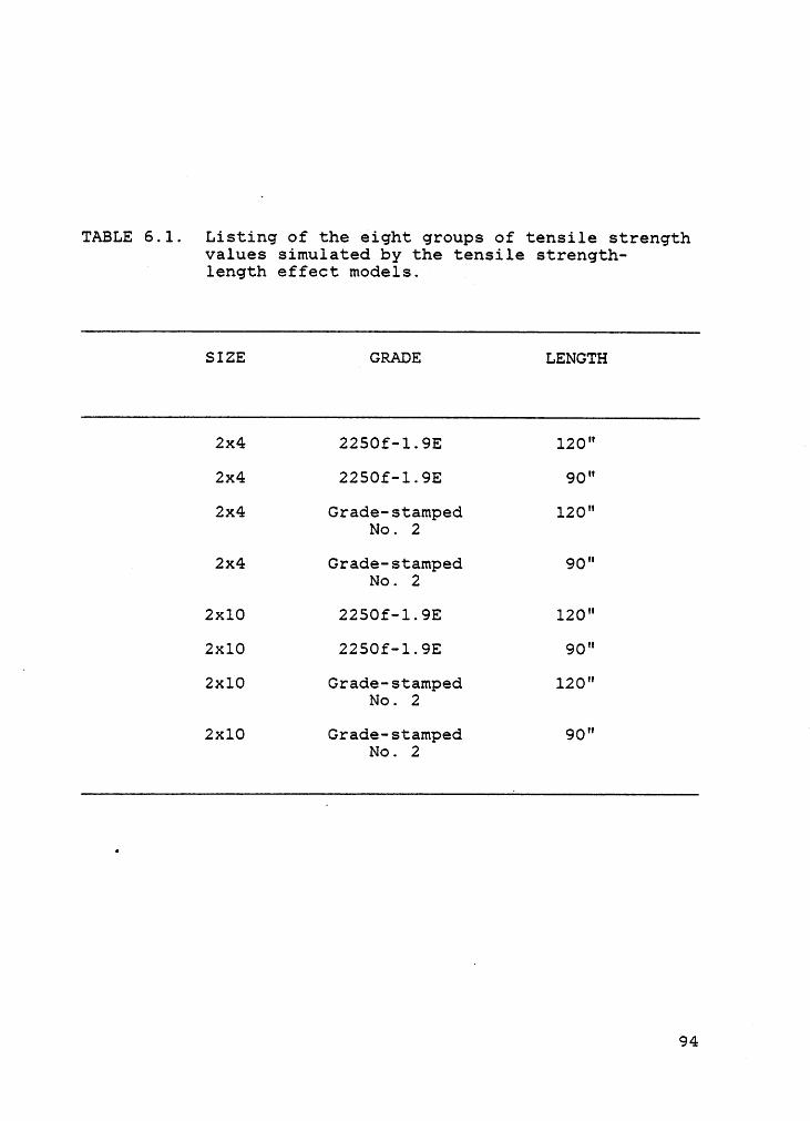
TABLE 6.1. Listing of the eight groups of tensile strengthvalues simulated by the tensile strength-‘ length effect models.

SIZE GRADE LENGTH

2x4 2250f-l.9E 120"2x4 2250f-1.9E 90"2x4 Grade-stamped 120"

No. 22x4 Grade-stamped 90"

No. 22xlO 2250f-1.9E l20"2xlO 2250f-1.9E 90"

A2xlO Grade—stamped l20"

No. 22xlO Grade-stamped 90"

No. 2

94

•-•I

>&_ Iggg .

EQ N • 1994 Lognormal ParametersI

>< *, Ä •8.98QÄ;

rc =· 0.268 1

I>_ .g I I(\j IDG . ~

I_ LI.6 I . ‘L‘ I

‘-Q '? —Il Is.@0 5.0 10.0. 15.0 20.0

Tensile Strength (1000 psi)

Figure 6.1 A lognormal distribution is superimposed onto the histogramof the generated tensile strength values from the lengtheffect model of the 90" 2::4 2250f·1.9E MSR Southern Pine.

95

I9*gg.N

E3 N - 1995 Lognormal ParametersA

Ä * l‘ co_§ C · 0.257. . 1 ·>— 1E1.1.1** IÜ 1 |L1.!01 1L1.,

°9‘CDÄ

EO i §....@0 5.0 10.0 15.0 20.0

V Tensile Strength (1000 psi)

Figure 6.2 A lognormal distribution is superimposed onto the histogramof the generated tensile strength values from the lengtheffect model of the 120" 2x4 2250f-1.9E MSR Southern Pine.

96

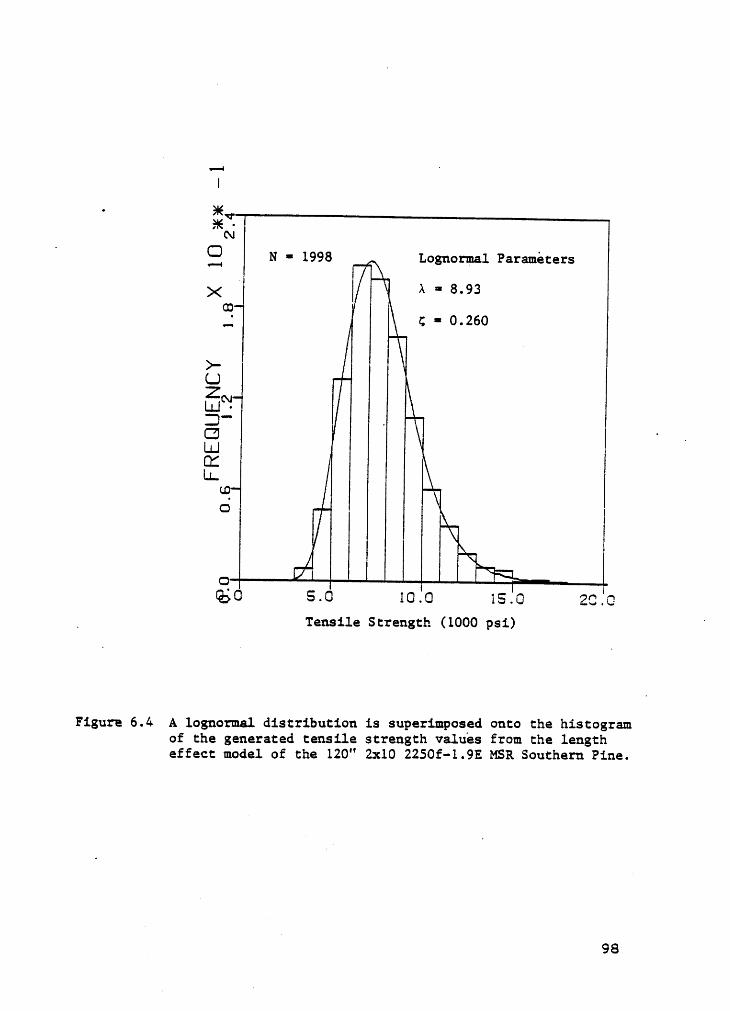
I.cu

N = 1998 4* Lognormal Parameters

Xl Ä * 8.93

I

,.Z C = 0.260. I IE10** ÄT IE I 9OSL1.ua

[ ‘LAV U:.

@0 5.0 10.0 15.0 2*.3.0_ Tensile Strength (1000 psi) ’

Figure 6.4 A lognormal distribution is superimposed onto the histogramof the generated tensile strength values from the lengtheffect model of the l20" 2x10 2250f—1.9E MSR Southern Pine.

98

IBK

Gu(D

><·v• A^I 1

>—‘2’LLILQ(Z5UJÜ: IU.G? ‘

L 1IJ W W.@$0 5.0 10.0 15.0 20.0

Tensile Strength (1000 psi)

Figure 6.6 A lognormal distribution is superimposed onto the histogramof the generated tensile strength values from the lengtheffect model of the 120" 2:4 No. 2 KD15 Southern Pine.

100

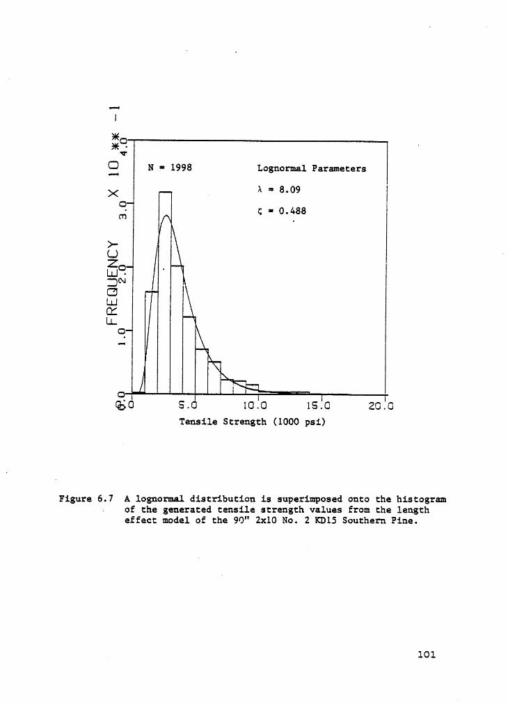
vr!

IXaeeq ·v

N = 1998 Lognormal Parameters

X _ Ä = 8.09 IQcr; C = 0.6188>— ·DNC1L1.!OSLI.C2

C2@0 5.0 10.0 15.0 20.0

'1'ensile Strength (1000 psi)

Figure 6.7 A lognormal distribution is superimposed onto the histogram. of the generated tensile strength values from the length

effect model of the 90" 2xl0 No. 2 KD15 Southern Pine.

„ lOl

U s-

BK9K · . .V .Q2 N - 2000 Lognormal Parameters

X · Ä4= 8.01Q 0 ass 1 1CO C ° 4

-L)Z|__‘_| .DN . . . 4. ClLe.!1 01L1. A

. ‘ u

‘ •.@05.0 10:0 15.0 1 20.0Tensile Strength (1000 psi)

Figure 6.8 A lognormal distribution is superimposed onto the histogramof the generated tensile strength values from the lengtheffect model of the 120" 2xlO No. 2 KD15 Southern Pine.

' 102

_ the lognormal distribution fit the generated tensile strength”

values for each of the eight cases under study.

. Figures 6.9 through 6.16 show relative frequency

histograms of the tensile strength of the 90-inch and

120-inch groups. The model generated tensile strength-length

effect probability curves are superimposed onto histograms

of the actual test data. A visual appraisal indicated that

the models adequately describe the data. Ix Kolmogorov-

Smirnov goodness-of-fit test was conducted on the eight sets

of test data and model generated probability curves, and the

only case to be rejected at the 5 percent significance level

was the case of the 2x10 MSR 120-inch lumber (Figure 6.12).

Using a goodness-of-fit test at the 5 percent signif-

icance level indicates that a true hypothesis is rejected,

on the average, 5 out of 100 tests, or, 1 in about 20 tests.

In this study, 1 out of 8 cases was rejected (2x10 MSR

120-inch). Therefore, it is very possible that the

Kolmogorov-Smirnov goodness-of-fit test in this case rejected

a true hypothesis.

Table 6.2 lists a comparison of the lag-3 serial corre-

lation estimated from 30-inch segments 1 and 4 tested and the

lag-3 serial correlation calculated from the model generated

120-inch pieces of lumber., Tensile strength values generated

for the first and fourth segments of the l20·inch piece of

lumber were used to determine the lag-3 serial correlation

103

zßq

1.8 Ä>-LJ „ 0Z|_,_| 1.2D

-

LUg 1'·‘· 0.8 Ä LYÜ! II• 0•ÜÄUL

T I MQTE TENS I ON (1000 P5 I)

Figure 6.9 The histogram of the ultimate tension of the 2xl+ 2250f-1.9EMSR 90" treatment group is shown. The model generatedtensile strength ·· length effect probability curve issuperimposed onto the histogram.

104-

I 2lq

V1.8.>_

IzLIJ 1.22cs~ 0.1¤= 1 L'·“ 0.6 ,‘

M, A .h;=._.I I "0.0 0.0 6.0 12.0 16.0ULTIMQTE TENSION (1000 PSI)

- •Figure 6.10 The histogram of the ultimate tension of the 21:42250f—l.9E MSR 120" treatment group is shown. Themodel generated tensile strength ·· length effectprobability curve is superimposed. onto the histogram.

' 105

2Iq

1I>-UZLL; 1. 2

_ DC5 '

O: .'·'· 0.6 ‘

0.0 *1.0 8.0 12.0 16.0UL T I MFITE TEN5 I 0N (1000 P5 I J

‘Figure 6.11 The histogram of the ultimate tension of the 2::10

I

2250f-1.9E MSR 90" treatment group is shown. Themodel generated tensile strength · length effectprobability curve is superimposed onto the histogram.

T „ 106

208

2.1 1>, Ä1.)Z „ .LI_|l.•·l3 .CJLu0:‘·'·0.7 ‘

"H IPmo_

Ä0.011.0 0.0 12.0 16.0ULTIMQTE TENSION (1000 PSI)

Figure 6.12 The histogram of the ultimate tension of the 2xlO2250f-1.9E MSR 120" treatment group is shown. Themodel generated tensile strength - length effectprobability curve is superimposed onto the histogram.

107

3.6

20 7

>-LJZLL] 1.8\GI.1J0:L'- 0. 6

I IIlh...e_.10.0 11.0 8.0 12.0 16.0

ULTIMPTE TENSION (1000 PSI) _

‘Figure 6.13 The histogram of the ultimate tension of the 2::4No.90"treatment group is shovm. The model generated

tensile strength · length effect probabilitv curve issuperimposed onto the histogram.

108 J

' 306l

2.7U.ZU 1.8‘

DOu.:VL" 0.9V0.0

*4.0 8.0 ' 12.0 16.0UL T I MFITE TENS I 0N (1000 P5 I)

Figure 6.14 The histogram of the ultimate tension of the 2x4 No. 2120" treatment group is shown. The model generatedtensile strength ·-- length effect probability curve issuperimposed onto the histogram.

6109

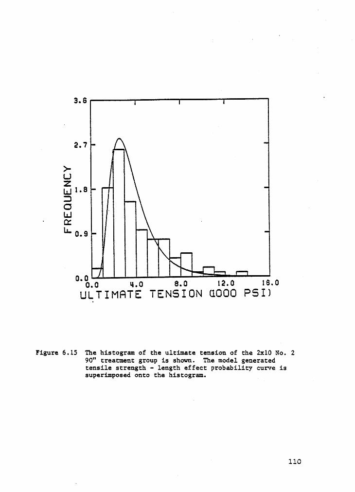
2I7

‘‘2’LL} 1.8DO

LI-I‘0:'·'· 0.s

11.0 8.0 12.0 16.0ULTIMPTE TENSION 11000 PSI)

Figure 6.15 The histogram of the ultimate tension of the 2xlO No. 290" treatment group is shown. '1'he model generatedtensile strength — length effect probability curve issuperimposed onto the histogram. _

° 110

*1.0 T T

3.0 ?

>-U ‘ · '

LU 2. 0 ‘B TG1 Ln.!T 0: 1L'- 1.00.0

*4.0 T. 8.0 12.0 18.0ULTIMRTE TENSION (1000 PSI)

- 5—F':Lgure 6.16 The histogram of the nltimate tension of the 2xlO No. 2T120" treatment group is shown. The model generated

T tensile strength — length effect probability curve isL T superimposed onto the histogram. ·

T1 lll

TABLE 6.2. Lag-3 serial correlation of tensile strength bysize and grade.

SIZE GRADE ACTUAL MODEL

2x4 2250f-1.9E 0.444 0.4532x4 Grade-stamped 0.831 0.631

No. 2

2xlO 2250f-1.9E 0.402 0.362 „

2xlO Grade-stamped 0.589 0.399No. 2

y 112

of the model. No glaring differences can be found in the

comparison of the model and the actual test data.

The fifth percentile values of tensile strength were

also compared between the model and the actual data. The

fifth percentile values were calculated assuming a lognormal

distribution. Table 6.3 lists the fifth percentile values

for the model and the tensile test data. Again, the values

generated from the model appear to agree well with the actuall

data, especially if one considers the small sample sizes used

to estimate the test data based fifth percentile.

113

TABLE 6.3. Fifth percentile values of tensile strength inpsi by size and grade.

- SIZE GRADE LENGTH ACTUAL‘ MODEL

2x4 2250f-1.9E l20" 4533 49822x4 2250f-1.9E 90" 4749 51022x4 Grade—stamped 120" 2103 1866

No. 22x4 Grade—stamped 90" 1995 1855

No. 22x10 2250f-1.9E 120" 4733 49022x10 2250f-1.9E 90" 5039 50312x10 Grade—stamped l20" 1025 1421

No. 22xl0 Grade—stamped 90" 1230 1456

No. 2

‘Assuming log—normal distribution

114

CHAPTER VII. APPLICATION OF THE LENGTH EFFECT MODEL

The following discussion relating to the "In-Grade"

program gives one immediate application of the tensile length

effect research. There are other applications in the areas

of truss design and glued-laminated beam research. However,’

these latter applications require improvements in load models

and are generally of a more complex nature requiring struc-

tural analysis.

7.1 DEVELOPMENT OF A TENSILE STRENGTH LENGTH ADJUSTMENT

The grading agencies participating 111 the "In-Grade"

testing program have been testing the ultimate tensile

strength of lumber at an 8—foot gage length and a 12-foot

gage length. It has been shown that length of a tensile test

span has significant effect on the ultimate tensile strength

of structural lumber. The results obtained by the grading

agencies are therefore influencmd by the test length and

cannot be compared directly. It may be useful to adjust the

ultimate tension value at the gage length tested to the cor-

responding ultimate tensLm1 if the piece was tested at a

standard length in order to compare and compile results. A

tensile strength length adjustment model was developed to

115

adjust the 5th percentile tensile strength at any gage length

to the corresponding 5th percentile tensile strengda at a

standard length for two grades and two sizes of Southern Pine

lumber. The 5th percentile strength was chosen because of

its use in the derivation of allowable design stresses.

The data base used to develop the tensile length ad-

justment model included 2x4 and 2x10 2250f—1.9E and 2x4 and

2xlO No. 2 KD15 Southern Pine. These four groups each ine

clude three test length groups, a 30-inch gage length, a

90-inch gage length and a l20·inch gage length. A lognormal

distribution was seen to be the best fit for each of the four

test groups and the 5th percentile tensile strength was es-

timated for subsequent use in developing the tensile length

adjustment model.

A standard length of 120 inches was selected since it

was recommended in the In-Grade planning documents and the

data base contained 5th percentile strength values at a

120-inch gage length. In addition, the maximum effective

buckling length·to·depth ratio for tension members in truss

design shall not exceed 80 (Truss Plate Institute, 1978).

A11 lumber used in the In-Grade testing program and in most

truss design has a minimum nominal dimension of 2 inches,

resulting in a maximum allowable length of 120 inches. Also,

foreseeing that a length adjustment might be applied to all

species in the In-Grade tension testing program, a standard

116

length of 120 inches is between the 8—foot and 12·foot gage

lengths currently being used.

Since the longest test gage length was 120 inches, it

was felt that more data of some form was needed to avoid an

unreasonable extrapolation for longer lengths. A 5th

percentile tensile strength at 300 inches was chosen as a

desired upper limit of length in order to make the model ap-

plicable for length adjustments for all lengths of solid—sawn

Southern Pine lumber. The 5th percentile tensile strength

of a 300 inch specimen was predicted from the tensile

strength-length effect model which generates ultimate tensile

strength of'za piece of Southern Pine lumber based on the

strength of a 30—inch piece.

The data base now includes four data points for each of

the four grade and size groups, three from actual data and

one predicted value for a 300-inch specimen. These points

were converted to length adjustment factors by dividing each

Sth percentile tensile strength by the corresponding 120—inch

5th percentile tensile strength. The length adjustment is

denoted by Equation 7.1.

Y = T(.)/T(120") (7.1)

where T(.) = 5th percentile tensile strength atany length

T(l20") = 5th percentile tensile strength at120 inches

117

The sample sizes, 5th percentile tensile strengths and length

adjustments for each grade and size group are given in Tables

7.1 through 7.4.

Tables 7.3 and 7.4 list model generated 5th percentile

tensile strength values for the 300 inch length which are

significantly higher than the tensile strength values at the

120 inch length calculated from the test data for the 2x4 and

»2x10 No. 2 KDl5 Southern Pine lumber groups. However, it has

been determined that tensile strength decreases with in-

creasing length. This anomoly of an increase in tensile

strength from 120 inches to 300 inches may be attributed to

an overprediction by the tensile strength-length effect

model, or the test data may not be representing the actual

behavior of tensile strength at 120 inches due to sampling

error. Also, increase in tensile strength from 120 inches

to 300 inches may be attributed to both an overprediction of

the model and a misrepresentation of the test data. There-

fore, the data obtained for the 2x4 and 2xl0 No. 2 KD15

Southern Pine lumber groups will be used to develop a tensile

length adjustment model since they are the best estimates of

the tensile strength behavior available.·

The length data exhibit a non-linear decrease ixz the

length adjustment with increasing length. This would be ex-

pected according to the asymptotic theory of statistical ex-

tremes (Ang and Tang, 1984). As illustrated in Ang and Tang

(1984), the distribution of values of the smallest value in

_ 118

Table 7.1. 5th percentile tensile strength and lengthadjustment, Y, for 2x4 2250f—1.9E Scuthern Pine.

Length Sample 5th percentile(inches) Size Tensile Strength Y(psi)

30 100 5470 1.20790 98 4749 1.048

120 100 4533 1.000300 NA 4547* 1.003

iM0del generated.

119

Table 7.2. 5th percentile tensile strength and lengthadjustment, Y, for 2xlO 2250f—1.9E Southern Pine. .

Length Sample 5th percentile(inches) Size Tensile Strength Y(psi)

30 100 5692 1.20390 98 . 5039 1.065

120 99 4733 1.000300 NA 4476* 0.946

IModel generated.

120

Table 7.3. 5th percentile tensile strength and lengthadjustment, Y, for 2x4 No. 2 KDl5 Southern Pine.

Length Sample 5th percentile(inches) Size Tensile Strength Y(psi)

30 98 2285 1.08690 98 1995 0.949120 98 2103 1.000300 NA 1685* 0.801

*Model generated. _

121

Table 7.4. 5th percentile tensile strength and lengthadjustment, Y, for 2x10 No. 2 KDl5 Southern Pine.

Length Sample Sth percentile(inches) Size Tensile Strength Y

(psi)30 104 1679 1.64190 104 1230 1.202

120 101 1023 1.000300 NA 1230* 1.202

*Model generated.

122

a sample of size_n decreases as I1 increases. However, the

shift in distribution from one sample size to a larger sample

size becomes less dramatic as n increases. In a general

sense, the asymptotic theory of statistical extremes explains

the asymptotic behavior of the data as length increases.

The tensile length adjustment model that best describes

this length effect is the non~linear regression model given

by Equation 7.2.

Y=A+BxcX (7.2)

·where X = gage length in inches

Y = length adjustment for 5th percentiletensile strength

The least-square estimates of the parameters A, B and C

were computed using the data base for each grade and size

group. The resulting curve was then vertically translated

by adjusting A such that Y = 1 for X = 120". In this manner,

lumber tested in tension with a 10—foot gage length will not

be subject to any length adjustment. Table 7.5 shows the

estimated. parameters for each grade and size group. A

graphical interpretation of the tensile strength length ad-

justment model is given in Figures 7.1 through 7.4 along with

the actual data used to develop the model.

123

Table 7.5. Estimated parameters A, B and C of equation 2 forthe tensile length adjustment model

Lumber Group A B C

2x4 2250f—l.9E 0.980 0.470 0.9742x4 No. 2 KDl5 0.765 0.429 0.995

2xl0 2250f—l.9E 0.939 0.424 0.9842x10 No. 2 KDl5 0.995 2.463 0.949

1

1.50 °

1.25^ a' 1

· OY E 0.981 + 0.470(0.97l•)X

i · 4*

I-\

‘

..Ä ons1-

•

>·‘ · 10.50

0.0 80.0 120.0 180.0 2*-40.0 300.0LENGTH (INCHE5) 1

Figure 7.1 Length adjustment, Y, for 2xl+ 2250f—1.9E Southern Pine.A "1east—squares" curve was determined and then forced

4 through the point Y equals 1.0 for length equal 120inches. The three leftmost points are from tensiletest data while the rightmost point was simulated by atensile strength model.

125

1 O

I•

lX

CD Y • 0.941 + 0.424(0.984)[\| .•-Q B ·

\

iÜ!1-

|

>-ol0.0

60.0 120.0 160.0 2*40.0 300.0LENGTH (I NCHE51

Figure 7.2 Length adjustment, Y, for 2xlO 2250f·1.9E Southern Pine.A "least—squares" curve was determined and then forcedthrough the point Y equals 1.0 for length equal 120inches. The three leftmost points are from tensile test „data while the rightmost point was simulated by atensile strength model.

12.6

1050

1 0 _an•

_ _•w Q Y • 0.765 + O.429(0.995)X"' 1.00 ~P- L.

\

..Ä 0. vs|- _.I

0•0.0 80.0 120.0 180.0 2*·10.0 300.0

LENGTH (INCHES)Figure

7.3 Length adjustment, Y, for 2x4 No. 2 KD15 Southern Pine.A "least·squares" curve was determined and then forcedthrough the point Y equals 1.0 for length equal 120 _inches. The three leftmost points are from tensile testdata while the rightmost point was simulated by a ;tensile strength model.

127

1075 _·

1.50 _l

4

'‘ X .Q 1.25 Y • 0.995 + 2.463(0.949)

gl., B”

..

_ I-„ 0.75

>-

0.50 °0.0 I 60.0 ..120.0 180.0 2*40.0 300.0 ·

LENGTH (INCHE5)

·„ Figure 7.4 Length adjustment, Y, for 21:10 No. 2 @15 Southern Pine.A "least·squares" curve was determined and then forcedthrough the point Y equals 1.0 for length equal 120inches. The three leftmost points are from tensile testdata while the rightmost point was simulated by atensile strength model.

4 128

7.2 APPLICATIONS OF THE TENSILE STRENGTH LENGTH ADJUSTMENT

The tensile strength length adjustment model was devel—

oped to transform the 5th percentile tensile strength of a

piece of Southern Pine lumber to the equivalent 5th

percentile tensile strength at a standard length of 120

inches. Application of the model as it might be used in the

In—Grade testing program is demonstrated using the followinge

example.

A test is conducted to determine the ultimate tensile

strength of 2x4 No. 2 KD15 Southern Pine lumber at a gage

length <xf 12 feet or 144 inches. A distribution is fitted

to the tensile strength data and the 5th percentile tensile

strength is estimated. From Figure 7.3, the length adjust-

ment at 144 inches equals 0.97. To find the equivalent 5th

percentile tensile strength at 120 inches, the 144-inch 5th

percentile tensile strength is divided by the length adjust-

ment. Therefore, the 5th percentile tensile strength as if

it were tested at the standard length would be the calculated

5th percentile strength divided by the length adjustment.

T(120") = 5th percentile strengthat 120 inches

= T(144")/Y

where T(144") = 5th percentile strengthat 144 inches

Y = length adjustment at 144 inches= 0.97

129

The model can also be used to adjust the design value

of tension parallel-to-grain in a wood member with respect

to the length of the member. This adjustment is accomplished

simply by multiplying the length adjustment, Y, by the design

value of tensile strength at the standard length, in this

case 120 inches. For example, a standard panel in floor

truss design is 30 inches and the truss chord is a 2x4

2250f—1.9E Southern Pine. From Figure 7.1, Y = 1.19 at 30

inches. This means that the 5th percentile tensile strength

at 30 inches is 19 percent stronger than the 5th percentile

tensile strength at the standard test length of 120 inches.

In a floor truss the center panel is the most highly stressed

in tension; therefore, the impact on design could be signif-

icant. If all the panels across the bottom chord had an equal

level of high tensile stress, the previous statement would

not be valid since, in effect, the lumber subject to the high

tensile stress would be 28 - 30 feet.

In summary, a tensile length adjustment model was de-

veloped for possible use in the In—Grade tension testing

program to adjust the tensile strength tested at different

gage lengths tona single tensile strength if the test had

been conducted at a standard length of 120 inches. The model

determines length adjustments for two grades and two sizes

of Southern Pine lumber, 2x4 and 2x10'22S0f-1.9E and 2x4 and

2x10 No. 2 KD15. Also, an example was given pointing to the

application of the model in wood truss design where the

130

length of the member is taken into account when designing

t€I‘1SiO1’1 members .

131

CHAPTER VIII. SUMMARY AND CONCLUSIONS

8.1 SUMMARY

This study was designed to investigate the effect of

length on tensile strength parallel-to-grain in lumber. In

addition, a model was developed to generate tensile strength

values of lumber taking into consideration the length of the

_ piece of lumber. These objectives were accomplished by

testing two sizes (2x4 and 2xl0) and two grades (2250f-1.9E

and No. 2 KD15) of Southern Pine lumber having three differ-

ent test span lengths of 30, 90 and 120 inches. A sample of

approximately 100 specimens in each treatment group was

tested which was adequate for model development. The tensile

strengths in the 30-inch treatment groups were significantly

higher than the tensile strengths in the 90-inch and 120-inch

treatment groups for each grade and size.

Tensile strength and MOE data from the 30-inch treatment

groups were used to develop tensile strength-length effect

models for the four grade and size groups. An MOE variabil-

ity model (Kline et al, 1985) was modified and used to gen-

erate 30-inch segment MOE values for a piece of lumber. The

segment MOE values were inputted into a weighted least

squares regression model in which the residuals were assumed

to follow a first-order Markov process. The weighted least

132

squares regression model generated 30—inch segment tensile

strength values of the piece of lumber. Using the weakest—

link concept, the minimum segment tensile strength value was

selected as the tensile strength of the generated piece of

lumber.

When generating segment tensile strength values, the

probability of generating lower tensile strength values in-

creases as the number of segments, or the length of the lum—

ber, increases. Thus, the tensile strength-length effect

model predicts a lower tensile strength for a longer piece

_ of lumber.The data base and resulting model were used to define a

length adjustment factor for tensile tests having different

gage lengths. For practical reasons a standard tension test

gage length of 10 feet was chosen.

8.2 CONCLUSIONS

For two sizes and two grades of Southern Pine lumber,

MOE and tensile strength of segments along the length of a

board were found to follow a parallel Markov process. A

modified version of the MOE variability model (Kline et al,

1985) was necessary to model segment MOE. The MOE variabil—

ity model is a second—order Markov process. Segment tensile

strength was found to follow a parallel first-order Markov

process. The two Markov processes were linked by a weighted

133

least squares regression model involving segment tensile

strength as the dependent variable and segment MOE as the

independent variable. This study showed that the tensile

strength distribution of lumber 90 and 120 inches long can

be adequately modeled from 21 statistically based knowledge

of the MOE and tensile strength characteristics of 30 inch

lumber segments.

It was concluded that the tensile strength-length effect

cannot be modeled by assuming the lengthwise segments of a

lumber specimen are non-correlated. A model using weibull's ·

"weakest-link theory" (Weibull, 1939) in which the segments

are assumed to be independent was found to inadequately de-

scribe the tensile behavior of a lumber specimen„ An inde-

pendent segment model underpredicts the tensile strength of

a lumber specimen.

The tensile strength-length effect model which was de-

veloped by allowing a regression of tensile strength on MOE

to account for the serial correlation in MOE and its result-

ing impact on tensile strength was also rejected because of

its inability to adequately describe the test data. In this

correlated segment model, the only correlation between

30-inch segments in predicting tension was derived from the

correlation of MOE between the segments. From the satisfac-

tory results obtained from the refined model, the serial

correlation in segment tensile strength parallel-to-grain is

134

higher than that predicted from the model using only serial

correlation in MOE.

The data base for the study was limited in scope and

size. Larger samples, other commercial grades and species

groups should be studied to verify the tensile strength-

length effect as being a parallel Markov process and to im-

prove on the estimates of the model parameters.

135

AEPENDIX A. PiROGRAM‘@LISTING OF THE MODIEIED MOE VARIABILITYMODEL. ‘ E

E l E1 136

Cu

SUBROUTINE LENMOE(DSEED,E,NS,N,LC,VMOE,IR)

3***********************************************************************3***** _*****0***** SUBROUTINE LENMOE TAKES AN INPUT ARRAY OF THE AVERAGE *****0***** MOE FOR A LUMBER SPECIMEN AND DETERMINES THE LENGTHWISE *****0***** VARIABILITY IN MOE. THE MOE FOR 30·INCH SEGMENTS ARE *****0***** FOUND FOR ANY SPECIMEN LENGTH. 4 DIFFERENT SIZES AND *****0***** GRADES OF LUMBER CAN BE CONSIDERED: Ag 2X4 225OF·l.9E *****0***** MSR LUMBER Bg ZX4 NO. 2 KD15 SOUTHERN INE LUMBER *****0***** CA 2X10 2250 ·1.9E MSR LUMBER AND D) 2X10 NO. 2 KD15 *****0***** S UTHERN PINE LUMBER. ‘ *****3***** *****3***********************************************************************0C THE STANDARD NORMAL RANDOM NUMBER GENERATOR GGNML FROM THE

E IMSL ROUTINE LIBRARY (1982) IS USED.C DSEED = INPUTÄOUTPUT DOUBLE PRECISION VARIABLE ASSIGNED AC RANDO INTEGER VALUE IN THE EXCLUSIVE RANGEC (1.D0,2147483647.D0). DSEED IS REPLACED BY A NEWE VALUE TO BE USED IN A SUBSEQUENT CALL.0 E = AN INPUT VECTOR OF DIMENSION NS OF RANDOM OBSERVATIONSE OF MOE FROM THE APPROPRIATE DISTRIBUTION. .g NS = THE NUMBER OF SPECIMENS (INPUT).

EN = THE NUMBER OF 30•INCH SEGMENTS PER SPECIMEN (INPUT).

g LC = IF INPUT = 1 · OUTPUT = MOE gg ZX4 225OF·l.9E MSRC IF INPUT = 2 · OUTPUT = MOE OF ZX4 NO. 2 KD15C SOUTHERN PINE LUMBER8 IF INPUT = 3 · OUTPUT = ägäßgä 2X10 225OF·l.9E MSRC IF INPUT ¤ 4 • OUTPUT = MOE OF 2X10 NO. 2 KD15S SOUTHERN PINE LUMBERC VMOE = THE OUTPUT MATRIX OF VARIABILITY IN MOE FOR EACHE SPECIMEN WITH DIMENSION NS BY N.C IR 3 THE NUMBER OF SPECIMENS REJECTED DUE TO SPECIFIEDS MAXIMUM AND MINIMUM MOE VALUES (OUTPUT).

E***********************************************************************C A MINIMUM SEGMENT MOE EMIN AND A MAXIMUM SEGMENT MOE, EMAX,C ARE GIVEN TO AVOID THE GENERATION OF UNREALISTIC SEGMNT MOE0 VALUES USING THE MARKOV MODEL. EMIN AND EMAX ARE THE MINIMUMC AND MAXIMUM SEGMENT MOES FOR THE FOUR DATA SETS OF 2X4 AND 2X10g 225OF·l.9E MSR AND NO. 2 KD15 SOUTHERN PINE.C IF A GENERATED SEGMENT MOE OF A SPECIMEN IS NOT IN THEC SPECIFIED RANGE AS INDICATED ABOVE ANOTHER SERIES OF SEGMENTMOE VALUES IS GENERAIED FOR THAT SPECIMEN.g*********************************************************************** °

DIMENSION X 110 E(NS VMOE(NS N)Cmoußm8ALL PARAMETERS ARE SPECIFIED

CGO TO (1,2,3,4),LC ·

g THE PARAMETERS FOR ZX4 225OF·l.9E MSRl 137

1 RESD = 0.377SE+06GBAR = 0.2S71E+07B1 = 0.6308% T 8 888EMIN = 0:1579E+07EMAX = 0.3623E+07C GO TO Sg THE PARAMETERS FOR ZX4 NO. 2 KD15

2 RESD = 0.507SE+06 ·GBAR = O.1749E+O7B1 = 0.606

2 • ·8% T 8 828EMIN = 0.4610E+06EMAX = O.3245E+07C GO TO SE THE PARAMETERS FOR 2X10 22SOF·1.9E MSR

3 RESD = 0.3601E+06GBAR = 0.2402E+07B1 = 0.8178% T 8 888EMIN = 0:1679E+07 ·EMAX = 0.3630E+07

C GO TO SE THE PARAMETERS FOR 2X10 NO. 2 KD15

4 RESD = 0.6006E+06GBAR = 0.1770E+07B1 = 0.816= .88 T 8882EMIN = 0.5280E+O6

C EMAX = 0.3236E+07g THE SECOND ORDER MARKOV MODEL GENERATES LENGTHWISE MOE

5 M = N + 10IR = ODO 100 J = 1,NS9 XE1; = 0.0

Dä ¥0 I = g°gCALL GGNML (DSEED 1 TgXRES = RESD * T 8 éo Til.0 · R2)XMARK = B2 * X(I) + B1 X(I+1)

XMARK + XRES10 C25; NU§ O¤o 11 1 ä= 11,11X(I-10g = X(I2 + GBAR11 8111888118 ““ T X I°‘°’118°88R1T-S8"é'TL°^“"”’

VMOE(J I2 é X(Ig/PCBAR * ECJ)IF (VMÖE J I).G .EMIN.AND.VMOE(J,I).LE.EMAX) GOTO 12112 = 112 + 1GOTO 9 ’12 CONTINUE ·100 CONTINUERETURN

138

END

139

APPENDIX B. PROGRAM LISTING OF THE TENSILE STRENGTH—LENGTHEEFECT MODEL. l

140

THIS ROUTINE GENERATES SETS OF LENGTHWISE 30·INCH TENSILE *****C***** STRESS VALUES GIVEN THE DISTRIBUTION OF THE AVERAGE MOE *****C***** OF A LUMBER SPECIMEN. THE ULIMATE TENSILE STRESS OF THE *****C***** SPECIMEN IS THEN DETERMINED USING A WEAKEST LINK THEORY *****g***** WHERE THE LINK TENSILE VALUES ARE SERIALLY CORRELATED. *****C***** USES SUBROUTINE LENMOE AND THE ROUTINES GGNML AND GGUBS *****C***** FROM THE IMSL ROUTINE LIBRARY(1982).C

C ECMAX = EMAX · 300000.0 PSI WHERE EMAX IS THE MAXIMUMSEGMENT MOE SPECIFIED IN SUBROUTINE LENMOE.C ECMIN = EMIN + 300000.0 PSI WHERE EMIN IS THE MINIMUMSEGMENT MOE SPECIFIED IN SUBROUTINE LENMOE.C CAUTION: IN ANY CASE ECMIN MUST BE GREATER THAN EMIN SPECIFIEDC IN SUBROUTINE LENMOE AND ECMAX MUST BE LESS THAN EMAXSPECIFIED IN SUBROUTINE LENMOE.C EPR = A VECTOR OF DIMENSION NR OF RANDOM OBSERVATIONSOF PIECE·AVERAGE MOE FROM THE APPROPRIATE DISTRIBUTION.uC T = A MATRIX OF 30•INCH TENSILE STRENGTH VALUES FOR NRC SPECIMENS WITH DIMENSION NR BY N. N·IS THE NUMBER OFDESIRED 30-INCH SEGMENTS PER PIECE OF LUMBER.C TS = A VECTOR OF DIMENSION NR OF ULTIMATE TENSILESTRENGTH OF EACH‘SPECIMEN.

DOUBLE PRECISION DSEED .DIMENSION EPR(2000),VMOE(2000,20),T(2000,10),VRES(2000,20),SC(9),

CCTS(2000)

C NUMBER OF SPECIMENSC NR=2000C §UMBäR OF 30·INCH SEGMENTS DESIRED.

3C M=N+10C DSEED = 950348.00C ä§LECZION OF SIZE AND GRADE OF LUMBER

3CC

GOTO (1,2,3,4) LTTHE PARAMTERS FOR THE ZX4 2250F•1.9E MSR

C MOE PARAMETERS1 ECMIN = l.879E+06ECMAX = 3.323E+06‘ XLAMDA = 14.75ZETA = 0.13298C REGRESSION PARAMETERSXK = 0.257S86024E·07B0 = O.81379013lE+01Bl = 0.3814ll61OE•06

C RESIDUAL CORRELATION .R03 = 0.39737C GO TO SC THE PARAMETERS FOR THE ZX4 NO. 2 KD15

141

CC MOE PARAMETERS2 ECMIN = 0.761E+06ECMAX = 2.945E+06EPS = 0.5221550E+06SIG = 1.3784885E+06NU = 2.6894493C REGRESSION PARAMETERSXK = 0.629349302E-07B0 = 0.727360916E+01B1 = 0.744034367E-06C RESIDUAL CORRELATIONRO3 = 0.56002C GO TO 6E THE PARAMETERS FOR THE 2X10 2250F·1.9E MSRC MOE PARAMETERS3 ECMIN = 1.979E+06ECMAX = 3.330E+06XLAMDA = 14.68ZETA = 0.13502C REGRESSION PARAMETERSXK = 0.333599424E-07B0 = O.848429012E+01B1 = 0.258614875E·06C RESIDUAL CORRELATIONRO3 = 0.32111 .C GO TO 5g THE PARAMETERS FOR THE 2X10 NO. 2 KD15C MOE PARAMETERS4 ECMIN = 0.828E+06ECMAX = 2.936E+06EPS = 0.3449451E+06SIG = 1.6037426E+06NU = 2.6883287C REGRESSION PARAMETERSXK = 0.930342026E·07B0 = 0.715514374E+01B1 = 0.716911018E·06C RESIDUAL CORRELATIONRO3 = 0.028605GO TO 6SC THE AVERAGE MOE VALUES ARE GENERATED AND A NEW MOE VALUE ISg GENERATED IF THE MOE EXCEEDS ECMIN OR ECMAX.5 D0 10 I=1 NR7 CALL GGNML(DSEED,1 R)EPR 1% = EXP%XLAMDA + R*ZETA

IF .ECMIN.OR.EPR(I .GT.ECMAX) GO TO 710 CO 16 gg I6 1 NR11 CALL GGUBS§DSEED 1 RgEPR€1g = S G*(·ALOG( &)**§1.§Ng% + EPS15 .EP (I . .ECMAX) GO TO 1116 CALL LENMOE(DSEED,EPR,NR,M,LT,VMOE,IR)Cg GENERATE T USING WEIGHTED LEAST SQUARES REGRESSION.

3äälgä ¥°ä’"§§" ’°‘ ’TS(I) = 100000.0

142

5 VRESSI 1) = 0.0· · 5 § 2E V 11 Lo J = 2,éM ·{ 2 =CALL GGNML(DSEED,1,Rg 2 ' ° AI ~ SIGI = SQRT§XK * VMO I,J))A V SIGK = SQRT XK * VMOE I Jwl gu · · I ·I 2EP = RO1 * SIGI/SIGK ÜRES J—1& V ; —ol * O1) 2 I

40 CONTINUE 1 I · I ä 52 ‘”éA DO 60·J=l1 M2 ¤ I -2 I I 5

I MC E T(I,J·10) = EXP(B0 + B1*VMOE(I,J) + VRES(I,J))I E HEAKEST LINK THEORY5 IF (T I,J•10).LT.TS(I)) TS(I) = T(I,J•10)i 2 30 CONTINUE . 5 2 Ü I ·5 5=C 4 TMAX IS THE MAXIMUM TENSILE STRENGTH FOR THE 30 INCH SEGMENTS·C FOR THE FOUR DATA SETS OF ZX4 AND 2X10 2250F·1.9E AND NO. 25 C Ü KDIS SOUTHERN PINE. A TENSILE STRESS VALUEIIS REJECTED IF IT ‘

4 I EXCEEDS TMAX.VTMAX= 17737.0 A2 2% A „1 ‘ IF §§S$I).GT.TMAX} GO TO 30 5 VA V 2 2 ' I2 ~ 5 I HRI { 6,200) TS( ) 3 I V’ 30 CONTINUE ‘ A ‘ 2 5 I

S THE SERIAL CORRELATION IS CALCULATED FOR LAGS 1 THRU MM 2DO 70 K=1 MM - A L :—4 2 F — I ,

I ·CALL SERCOR (T,TS,TMAX,K,N,N,SC(K))70 CONTINUEHRITE 7 300; (SC(K),K=1,MM) 5 ·2 200 FORMAT 10X F .0) · 2 · I I300 FORMAT 3F15.5) -5 ‘

A WRITE(8 400) R 5 I 2j A400_5 FORMATéI6 ' BOARDS HERE REJECTED;DUE TO SPECIFIED MINIMUM AND MAXIcmm Mo vL1.mas.·) 2

STOP _I I2 IC END V 7 5 _ ·- 5

Ii C SÜBRÜÜTTNE_SERcÜR CALCULATES THE SERIAL CORRELATIONS AT A IV C SPECIFIED LAG FOR EACH LUMBER SPECIMEN WITH ULTIMATE TENSILE2 STRENGTH LESS THAN OR EQUAL TO XMAX. ; 2 I

‘ 2 SUBROUTINE SERCOR(X XX XMAX K N~NX RK Üummvszou x(Nx,m,xicm’0 ’ ’ ’· ’· ) ·V 4 I g

2 ; T4-=0. 2 - j 2TS=0. 2 V° L=N·K 5 2 A„ M=NX~!cL IÜ DO 10 I=1,NX I I2 ' IF (XX$I).GT.XMAX) GO TO 10 =DO 20 =1,L A I 2T1=T1+X I,Jg*X(I,J+K) 4 5T2=T2+X I,2J2IT3=T3+X I,J+§l AIT4=T4+X I,J) 2TS=T5+X I,J+K)**2 ; _„ 5 °I 20 CONTI I 2 12 7 10 CONTINUE · " · 2T6= T1•T2*T3/FLOAT M I 5T7= T4•T2**2/FLOAT M **0.5 2 2 V A2 T8= T5·T3**2/FLOAT M **0.5 · A

2 I A 143

END

1 44

REFERENCES

Ang, A. H-S. and W. H. Tang. 1984. Probability concepts inengineering planning and design: Volume II. Decision,risk, and reliability. John Wiley and Sons, Inc. NewYork, New York. 562p.

Barrett, J. D. 1974. Effect of size on tensionperpendicular-to-grain strength of Douglas—fir. Wood andFiber 6(2): 126-143.

Bender, D. A. 1980. Fire endurance reliability formulationfor glued-laminated beams. Thesis submitted in partialfulfillment of the requirements for the degree of Masterof Science, Virginia Polytechnic Institute and State Uni-versity. Blacksburg, Virginia.

Bohannan, B. 1966. Effect of size on bending strength ofwood members. U. S. Forests Products Laboratory researchpaper FPL 56. Madison, Wisconsin.

Buchanan, A. H. 1983. Effect of member size on bending andtension strength of wood. Paper presented at I.U.F.R.0.Wood Engineering Meeting. Madison, Wisconsin. 31p.

Evans, J. W., R. A. Johnson and D. VV. Green. 1984. Esti—mating the correlation between variables under destructivetesting, or how to break the same board twice.Technometrics 26(3): 285-290. —

Foschi, R. 0. and J. D. Barrett. 1980. Glued—laminated beamstrength: A model. ASCE Journal of the Structural Divi-sion 106(ST8). _

Green, D. W., J. W. Evans and R. A. Johnson. 1984. Inves-tigation of the procedure for estimating concomitance oflumber strength properties. Womd Fiber Science 16(3):426-440.

Haan, C. T. 1977. Statistical methods in hydrology. IowaState University Press. Ames, Iowa. 378p.

Kline, D. E., F. E. Woeste and B. A. Bendsten. 1985.Stochastic modulus of elasticity of lumber. Wood and Fi-

‘

ber Science. In press.

145

Kunesh, R„ IL and J. W. Johnson. 1974. Effect of size ontensile strength of clear Douglas-fir and Hem-fir dimen-sion lumber. Forest Products Journal 24(8): 32-36.

Liu, J. Y. 1980. Shear strength of wood beams: A Weibullanalysis. ASCE Journal of the Structural Division106(ST10): 2035-2052.

Liu, J. Y. 1981. A Weibull analysis of wood member bendingstrength. In: F. T. C. Loo (ed.). Failure preventionand reliability. Society of Mechanical Engineers.pp57-64.

National Forest Products Association. 1982. National designspecification for wood construction: Structural lumber,glued-laminated ·timber, timber pilings, and fastening.National Forest Products Association. Washington, D. C.

Poutanen, T. 1984. Model for timber strength under axial ·load and moment. International Council for Building Re-search Studies and Documentation Working CommissionW18-Timber Structures. Rapperswil, Switzerland. 25p.

Trus Joist Corporation. 1979. Micro=lam headers and beams.Trus Joist Corporation. Boise, Idaho.

Truss Plate Institute. 1978. Design specification for metalplate connected. wood. trusses. Truss IPlate Institute.Madison, Wisconsin. 35p.

Weibull, W. 1939. A statistical theory of the strength ofmaterials. Swedish Royal Institute Engineering ResearchProceedings. Stockholm, Sweden.

Woeste, F. E., S. K. Suddarth and W. L. Galligan. 1979.Simulation of correlated lumber properties data - A re-gression approach. Wood Science 12(2): 73-79.

Yevjevich, V. 1972.” Stochastic processes in hydrology.Litho Crafters. Ann Arbor, Michigan. 276p.

146