-l copy - defense technical information center · abstract madaline rule ii, mrii, is a supervised...
TRANSCRIPT

-L COPY "w SECURITY CLASSIFICATION OF THIS PAGE
Form ApprovedREPORT DOCU MENTATION PAG E OMB No. 0704-0188
la. REPORT SECURITY CLASSIFICATION lb. RESTRICTIVE MARKINGSUNCLASSIFIED NONE
2 3. DISTRIBUTION/AVAILABILITY OF REPORTAPPROVED FOR PUBLIC RELEASE;
21 DISTRIBUTION UNLIMITED.
4. 5. MONITORING ORGANIZATION REPORT NUMBER(S)
AFIT/CI/CIA-89-029
6a. NAME OF PERFORMING ORGANIZATION 6b. OFFICE SYMBOL 7a. NAME OF MONITORING ORGANIZATIONAFIT STUDENT AT (if applicable) AFIT/CIAStanford UNIV I
6c. ADDRESS (City, State, and ZIP Code) 7b. ADDRESS (City, State, and ZIP Code)
Wright-Patterson AFB OH 45433-6583
Ba. NAME OF FUNDING/SPONSORING 8b. OFFICE SYMBOL 9. PROCUREMENT INSTRUMENT IDENTIFICATION NUMBERORGANIZATION (If applicable)
S ADDRESS (City, State, and ZIP Code) 10. SOURCE OF FUNDING NUMBERSPROGRAM PROJECT TASK WORK UNITELEMENT NO. NO. NO ACCESSION NO.
11. TITLE (Include Security Classification) (UNCLASSIFIED)MADALINE RULE II: AN INVESTIGATION
12. PERSONAL AUTHOR(S)Rodney G. Winter
13a. TYPE OF REPORT 13b. TIME COVERED 14. DATE OF REPORT (Year, Month, Day) 15. PAGE COUNTDR ISSERTATION FROM TO_ _ 1989 88
16. SUPPLEMENTARY NOTATION ARPROVD --RPBIC RELEAS lA AFR 190-1ERNEST A. HAYGOOD, 1st Lt, USAFExecutive Officer, Civilian Institution Proarams
17. COSATI CODES 18. SUBJECT TERMS (Continue on reverse if necessary and identify by block number)FIELD GROUP SUB-GROUP
19. ABSTRACT (Continue on reverse if necessary and identify by block number)
DTIC TELECTE
FEB 1 2 1990
20. DISTRIBUTION/AVAILABILITY OF ABSTRACT 21. ABSTRACT SECURITY CLASSIFICATIONrUNCLASSIFIEDIUNLIMITED 0 SAME AS RPT. E] DTIC USERS UNCLASSIFIED
22a. NAME OF RESPONSIBLE INDIVIDUAL 22b. TELEPHONE (Include Area Code) 22c. OFFICE SYMBOLERNEST A. HAYGOOD, 1st Lt, USAF (513) 255-2259 AFIT/CI
DD Form 1473, JUN 86 Previous editions are obsolete. SECURITY CLASSIFICATION OF THIS PAGE
AFIT/CI "OVERPRINT"

December 19, 1988
AFIT/CIRDWright-Patterson AFB, OH 45433-6583
Re: Clearance for publication
I request clearance for release of my dissertation, "Madaline Rule II: An Investiga-tion." This is a draft that has been submitted to my princi advisor. I expect onlyminor changes having no effect on the basic content to com'e-from him.
Please review as soon as possible. I expect to submit this dissertation in final formto the university on 9 Jan 89. Make sure any inputs you have reach me by 6 Jan 89.
RODNEY G. WINTER, Major, USAFInformation Systems LaboratoryStanford UniversityStanford, CA 94305
9 03

MADALINE RULE II:
AN INVESTIGATION
A DISSERTATION
SUBMITTED TO THE DEPARTMENT OF ELECTRICAL ENGINEERING
AND THE COMMITTEE ON GRADUATE STUDIES
OF STANFORD UNIVERSITY
IN PARTIAL FULFILLMENT OF THE REQUIREMENTS
FOR THE DEGREE OF
DOCTOR OF PHILOSOPHYAccesio; For
MIS C, by
By -
Rodney G. Winter ' ..
January 1989

O Copyright January 1989 by Rodney G. Winter
All Rights Reserved
ii

a
I certify that I have read this thesis and that in my opinion
it is fully adequate, in scope and in quality, as a dissertation
for the degree of Doctor of Philosophy.
Bernard Widrow(Principal Advisor)
I certify that I have read this thesis and that in my opinion
it is fully adequate, in scope and in quality, as a dissertation
for the degree of Doctor of Philosophy.
Joseph W. Goodman
I certify that I have read this thesis and that in my opinion
it is fully adequate, in scope and in quality, as a dissertation
for the degree of Doctor of Philosophy.
James B. Angell
Approved for the University Committee on Grauuate Studies:
Dean of Graduate Studies
iii

Abstract
Madaline Rule II, MRII, is a supervised learning algorithm for training layered feed-forward
networks of Adalines. An Adaline is a basic neuron-like processing element which forms
a binary output based upon a weighted sum of its inputs. The algorithm was developed
based on the minimal disturbance principle. This principle states that changes made to
the network to correct errors should disturb it as little as possible. A method to insure
all processing elements share responsibility for forming the global solution was introduced
and called usage. Details of the algorithm were developed with consideration for hardware
implementation. 4 -
Simulation results of MRII are presented. The algorithm exhibits interesting generaliza-
tion properties. Generalization is the network's ability to make correct responses to inputs
not included in the training set. Networks that contained more Adalines than necessary to
solve a given training problem exhibited good generalization when trained by MRII. The
algorithm was found to not always converge to known solutions. A failure mode of the
algorithm was identified and is detailed in this report.
The sensitivity of Madaline networks to random changes in weights and errors in in-
puts was investigated. Simple formulas were found to predict the average change of the
input/output mapping due to these effects. These results apply to networks where the
individual weights are selected independently from a random distribution.
iv

Preface
The guidance and direction of Dr. Bernard Widrow during the conduct of this research is
gratefully acknowledged. -His insistence for simplicity and clarity forced me to arrive at
simple results. He is largely responsible for any utility the results presented here have.
The support of Ben Passarelli of Alliant Computer Systems Corporation is also greatly
appreciated. Ben made available his company's equipment for performing many of the
simulations presented in this report. More importantly, he gave selflessly of his time to
teach me how to best use the equipment and make it available on weekends.
My colleagues in the "zoo" have been the source of much inspiration. Special thanks goes
to Maryhelen Stevenson who proofread much of this report before the reading commitee.
Her competence saved me some embarrassment.
During the period of this research, the author was an active duty officer in the United
States Air Force. He was assigned to Stanford University under the Civilian Institutes
Program of the Air Force Institute of Technology. No information or statement contained
in this report should be construed to be supported by or representative of the policies or
views of the United States Air Force.
v

Contents
Abstract iv
Preface v
1 Introduction 1
1.1 Contributions .......................................... 1
1.2 The Adaline ............................................ 3
1.3 Early Madalines ....... ................................. 6
1.4 Concept of Madaline Rule II - Minimal Disturbance ................ 12
2 Mathematical Concepts 16
2.1 Multi-Dimensional Geometry ....... .......................... 16
2.2 Hoff Hypersphere Approximation .............................. 19
3 Details of Madaline Rule II 23
3.1 Desired Features for a Training Algorithm ........................ 23
3.2 Implementing MRII ........ ............................... 24
3.3 Usage ......... ....................................... 31
4 Simulation Results 33
4.1 Performance Measures ..................................... 33
4.2 An Associative Memory ....... ............................. 35
4.3 Edge Detector ........................................... 36
4.4 The Emulator Problem ..................................... 41
5 A Failure Mode of MRII 45
5.1 The And/Xor Problem ..................................... 45
vi

5.2 A Limit Cycle ......... .................................. 47
5.3 Discussion ........ ..................................... 55
6 Sensitivity of Madalines to Weight Disturbances 58
6.1 Motivation ......... .................................... 58
6.2 Perturbing the Weights of a Single Adaline ..... .................. 59
6.3 Decision Errors Due to Input Errors ...... ...................... 64
6.4 Total Decision Errors for Adalines and Madalines .................. 73
6.5 Simulation Results ........ ................................ 75
6.6 Discussion ........ ..................................... 81
7 Conclusions 85
7.1 Summary ......... ..................................... 85
7.2 Suggestions for Further Research .............................. 86
Bibliography 87
vii

List of Tables
4.1 Performance for the edge detector problem. Averages are for training on 100
nets beginning at random initial weights ......................... 40
4.2 Training and generalization performance for the emulator application. The
fixed net was 16 input, 3-feed-3 ................................ 43
5.1 Truth table for the and/xor problem ............................. 47
5.2 The input pattern to hidden pattern to output pattern mapping for State 1.
Incorrect output responses are marked by * ...... ................... .... 48
5.3 The results of trial adaptations from State 1 ........................ 51
5.4 Mapping information for the network in State 2 ..................... 51
5.5 Mapping for the postulated State 3 ............................. 54
6.1 Effects of perturbing the weights of a single Adaline. The predicted and
simulated percentage decision errors for weight disturbance ratios of 5, 10,
20 and 30 percent are shown for Adalines with 8, 16, 30, and 49 inputs. . . 76
6.2 An output Adaline sees errors in its input relative to the reference network.
Predicted and observed frequency of each number of input errors and pre-
dicted and observed error rates for each number of input errors are presented. 78
6.3 Percent decision errors for a 16-input, 16-feed-1 Madaline with weight dis-
turbance ratios of 10, 20, and 30 percent ......................... 79
6.4 Simulation vs. theory for a multioutput Madaline. The network was a 49-
input, 25-feed-3. A decision error occurs when any bit of the output is
different from the reference .................................. 80
viii

List of Figures
1.1 The adaptive linear neuron, or Adaline .......................... 3
1.2 Graph of Adaline decision separating line in input 2-space ............... 5
1.3 Structure of the Ridgway Madaline ...... ....................... 3
1.4 Implementation of the AND, OR and MAJority logic units using Adalines
with fixed weights ........................................ 9
1.5 Ridgway Madaline realization of the exclusive-or function ........... ... 11
1.6 Graphical presentation of the Madaline of Figure 1.5. The Adalines map the
input space into an intermediate space separable by the OR unit ....... .. 11
1.7 A three layer example of the general Madaline ..... ................ 13
2.1 The differential area element of a hypersphere as a function of the polar angle
S. . . . . . . . . . . . . . . . . . . . . . . . . . . . . . . . . . . . . . . . . . 21
2.2 A lune of angle 0 formed by two bisecting hyperplanes ................. 22
3.1 Block diagram implementation of a Madaline trained by MRII ........ .. 25
3.2 Structure of a single layer within the network of Figure 3.1 ............ 26
3.3 Block diagram of the Adalines for Figure 3.2 ....................... 27
3.4 An Adaline modified to implement the usage concept ................ 32
4.1 Diagram of a translation invariant pattern recognition system. The adaptive
descrambler associates a translation invariant representation of a figure to
its original representation in standard position ..................... 37
4.2 Learning curves for patterns and bits for the adaptive descrambler associative
memory application. Average of training 100 nets. Data points are marked
by "o" ................................................ 38
4.3 A component of an edge detector system. The Madaline outputs the position
of the first black pixel in a binary code .......................... 39
ix

4.4 Training a network to emulate another. The fixed net provides desired re-
sponses for the adaptive net ....... ........................... 41
4.5 Tracking of generalization and training performances. Network is a 16 input
9-feed-3 emulating a 3-feed-3 fixed net ............................ 44
5.1 Graphical representation of a network that solves the and/xor problem. . . 46
5.2 Graphical presentation of State 1 ............................. 49
5.3 Graphical presentation of trial adaptations from State 1 ............... 50
5.4 Separation of the hidden pattern 3pace for State 2 .................. 52
5.5 An output separation that would give State 3 ...................... 53
6.1 Comparing a network with a weights perturbed version of itself ........ .. 59
6.2 Reorientation of the decision hyperplane due to a disturbance of the weight
vector. Patterns lying in the darker shaded region change classification. . . 61
6.3 Geometry in the plane determined by W and AW ................... 62
6.4 The nearest neighbors of )9 lie equally spaced on a reduced dimension hyper-
sphere ................................................. 66
6.5 All the patterns at distance d from 91 will be classified the same as X-1. Some
of the patterns at distance d from X2 are classified different from 92 ..... .. 67
6.6 A representation of the location of the patterns at distance d from the input
vector X . ......... ...................................... 68
6.7 A representation of the geometry in the plane formed by W and )9...... .. 69
6.8 Representation of the geometry in the hyperplane containing the patterns at
distance d from XZ. This hyperplane is the floor of thc shaded cap in Figure 6.6. 70
6.9 Sensitivity of the single Adaline. Dotted lines are simulation results for
Adalines with 8, 16, 30, and 49 inputs. Solid line is the theory prediction by
the simple approximation. Data is taken from Table 6.1 ................ 77
6.10 Percent decision errors versus percent weight perturbation. Network is a
16-input, 16-feed-1 Madaline. Theory predictions by two different levels of
approximation are shown with simulation results. Data from Table 6.3. . . 80
6.11 Decision Errors vs. Weight Perturbation Ratio for a multioutput Madaline.
Network is 49-input, 25-feed-3. Data taken from Table 6.4 ............. 81
x

6.12 Sensitivity of networks as nj is varied. The net used had 49 inputs, 1 output
Adaline and the percent weight perturbation ratio was 20%. Actual data
points for the simulation results are marked by "o" ................... 83
xi

Chapter 1
Introduction
Research in the field of neural networks has seen a resurgence of interest in the past several
years. Neural networks offer the hope of being able to teach a machine how to perform
a given task by showing it examples of sample behavior. Since the machine learns by
experience, the task at hand does not need to be decomposed into an algorithm that can
be programmed into the machine. This dissertation investigates a method by which a
particular type of neural network can be trained.
The neural network to be trained is a layered feed-forward Adaline network. The term
Adaline, which stands for "adaptive linear neuron," was coined by Widrow in 1959 [1]. The
original work presented in this report builds on the work done by Widrow and many of
his graduate students in the early 1960s. This introduction will review some of this past
work on Adalines and simple networks of Adalines, called Madalines for "many Adalines."
The concepts behind Madaline Rule II, which is a method for training more complicated
networks of Adalines, will also be presented.
1.1 Contributions
This dissertation presents two major contributions. The first is the Madaline Rule II algo-
rithm, MRII. The second is the sensitivity results presented in Chapter 6. There are some
minor contributions within these two major ones.
The Madaline Rule II, as the "II" suggests, is the result of continuing work started by
others. This introduction chapter will outline this previous work. First the Adaline will be
presented. Then a simple network of Adalines called a Madaline will be presented. This

CHAPTER 1. INTRODUCTION 2
early Madaline has a much simpler structure than that addressed by Madallne Rule II.
The procedures for training these two simple structures are grounded in a concept called
minimal disturbance. Minimal disturbance is a basic concept behind MRII and is the
author's inheritance from the early researchers. The last section of this chapter explains
a concept for training a complex Madaline using a sequence of trial adaptations. The
trials least disturbing to the network are to be performed first, in accord with the minimal
disturbance principle. This idea is presented by the author in greater detail than previously
published by other researchers in the last section of this chapter. Though more detailed,
the ideas presented there follow directly from previous work and the author claims no
contribution for them.
The author has taken the ideas left behind by the early researchers and made them work.
In formulating MRII, some changes to the minimal disturbance principle were required.
These changes are detailed in Chapter 3 and are the author's contributions. Real neural
networks need to be built in circuitry. This requirement molded the choices of which trial
adaptations to perform. Minimal disturbance also needed modification to insure all units
shared responsibility for arriving at a network solution. This was implemented by the author
as "usage" in the MRII algorithm. After discovering the need for and implementing usage,
the author discovered a similar idea had been proposed by another. This minor contribution
by the author appears to be independent but not original. The author's experimental results
with the algorithm are offered as a contribution as well as the several heuristics presented
for using the algorithm.
In working with MRII, the author discovered a failure mode of the algorithm. This
mode prevents the algorithm from coming to a solution even when a known solution exists.
This mode takes on the form of a limit cycle and is detailed in Chapter 5. The author
presents this as a contribution since an understanding of this phenomenon is essential to
improving the algorithm. An attempt to improve MRII by finding an escape to the failure
mode led the author to his second major contribution.
The sensitivity of the input/output response of Madalines to changes in the weights of
the system as well as to errors in the inputs to the system were analyzed. Approximations
were made to reduce the analytic results to useful form. These approximations were verified
for accuracy by experiment. The result is a useful and relatively easy to use set of equations
that accurately predict the sensitivity of "random" Madalines. These results should be a
worst case situation for Madalines that have been trained. The results should also be a
useful tool for further research into improving the MRII algorithm.

CHAPTER 1. INTRODUCTION 3
x 0 =+1 (bias input)
Input WeightsPattern w1w0
x .
2 w2 Analog
- +q
x3 - 1Binary
Threshold OutputDevice
Iw I
d Adaptive
desired Algorithm
response ADALINE
--- -------- -- - ----- _
Figure 1.1: The adaptive linear neuron, or Adaline.
1.2 The Adaline
The Adaline is an adaptive threshold logic unit and is depicted in Figure 1.1. The Adaline
performs a weighted sum of its inputs and makes a binary decision based on this sum.
The input to the Adaline has n variable components and compose what will be called
the input pattern. The input pattern along with the constant +1 bias input form the
(n + 1)-dimensional input vector R = [To = +l,z1 ,...,Xn]T. The input vector is the bias
augmented input pattern, a semantic distinction which will be followed throughout this
paper. The weighting vector is W = (wo, wi, ... , wn]T .The weighted sum, referred to as the
Adaline's analog sum or analog output, is the dot product of these two vectors, y = XT V.
The Adaline's binary output is the result of passing this analog sum through a threshold

CHAPTER 1. INTRODUCTION 4
device, q = sgn(y), where sgn(.) is +1 for positive argument, and -1 otherwise.
The individual components of the input vector could be any real analog values but often
are restricted to being binary. Except as noted, the input component values will be either
+1 or -1 in this paper. There are two reasons for making this restriction. First, this will
be the case when an Adaline is receiving its inputs from the outputs of other Adalines.
Secondly, with this restriction on the inputs, the magnitude of the input vector, 19,, will
be a constant v'7+T1. This will simplify the mathematical analysis to be presented.
The weights axe allowed to be continuous real valued numbers. From Figure 1.1 it is
noted that these weights are adjustable by an adaptive algorithm. The actual hardware
implementation of adjustable analog valued weights will not be specifically addressed in
this paper. This issue has been addressed in the past and resulted in the invention of a
device called a memistor [2]. Solid state implementations of adjustable weights are the
focus of much current research. It will be assumed here that such weights are available for
the eventual hardware realization of neural networks. The issue of how close these weights
have to be to their nominal values will be addressed later.
The Adaline is capable of making a binary decision based upon its inputs. What is
the nature of this decision making capability? This can be determined by examining the
Adaline's governing equation at its decision threshold, that is, when the analog sum y is
zero. For the case of an Adaline with two variable inputs this equation is:
Y = XT W- = WO + XlWl + X2W2 = 0.
This can be rewritten as:Wl WO
X2 = -- X1 - -•W2 W2
This is a straight line in the X1 -x 2 input space with a slope -W l /W 2 and X2-intercept of
-Wo/W2. An example plot of this equation is shown in Figure 1.2. The inputs to the right
of the separating line cause the analog sum to be positive, resulting in a +1 decision by the
Adaline. To the left of the line, inputs result in a -1 decision. The Adaline thus performs a
mapping from its multi-dimensional input space to its one-dimensional binary output space.
The input/output mapping effected by this example Adaline is represented by:
(+1,+1) +1
(+1,-i) +- +1 (1.1)
(-1,-i) +1

CHAPTER 1. INTRODUCTION
X2 w2 wf
w2 W(-1, +1) / (1,1)
DecisionSeparating
Line
©X
Figure 1.2: Graph of Adaline decision separating line in input 2-space.
(-I,+1) *- -1
By adjusting the weights, the orientation of the line in Figure 1.2 can be changed aswell as which side of the line results in a positive decision. This then can cause a change
in the input/output mapping of the Adaline. Methods for adapting the weights of a single
Adaline to achieve a desired input/output mapping were developed in the early 1960's.
The method for changing the weights is represented by the "adaptive algorithm" blockin Figure 1.1. The algorithm has as inputs the desired response, d, for the pattern being
presented and the actual analog response of the Adaline. Mays [3] summarizes three adap-tation procedures for the single Adaline. All three of these procedures will produce a set
of weights to provide the desired input/output mapping, if such weights exist, in a finitenumber of adaptations. An example of an input/output mapping that cannot be achieved
by a single Adaline will be shown later.
Mays' formulation of the adaptation procedures included a concept called the deadzone.In any hardware implementation of an Adaline, a real thresholding element will be used. If
the analog sum y is very close to zero, it is possible the thresholder could flip output states
in an erratic fashion due to noise. Manufacturing tolerances might also cause the actualthreshold to be different from zero. For these reasons it is desired that the magnitude of
the analog sum be greater than a deadzone value 6 > 0. The magnitude of the analog sumis referred to as the confidence level. It is a measure of how sure the Adaline is about its

CHAPTER 1. INTRODUCTION 6
decision. During training then, not only must the binary decision be correct, but it must
be made with a minimum confidence level equal to the deadzone.
All of the Adaline adaptation procedures can be summarized as follows. There exists
a set of patterns and associated desired responses that the Adaline is to learn. This set
is called the training set. Present a pattern and its associated desired response from the
training set to the Adaline. If the binary response is correct and the confidence level is
greater than the deadzone, go on to the next pattern. If the response is incorrect or not
confident enough, make a change in the weights. The weights will be changed by adding
or subtracting some portion of the input. The weight changing method for the modified
relaxation procedure is detailed here.
W(k + 1) = W*(k) for dX w(k) >6
- W(k) + n±dX[L - dx w(k)] for dxjvW(k) < 6 (1.2)
Here k is an adaptation counter so that V(k+1) are the weights after the kth adaptation. As
before, d is the desired binary response associated with the input vector ). The adaptation
constant, 77, must have value 0 < 77 < 2 to insure convergence. The deadzone can be
selected 0 < b < 1. The quantity L is called the adaptation level and is selected 6 < L.
The adaptation level can be thought of as a target confidence level when 77 = 1. To see
this, compute the resulting analog sum after adaptation by premultiplying both sides of
Equation 1.2 by X T . Remembering that y = XTV, and XTX = n + 1:
y(k + 1) = y(k) + rjd[L - dy(k))
= y(k)[1 - 771 + 77dL
= dL for 77 = 1.
After adaptation, the Adaline will provide the correct response with confidence equal to
the adaptation level when q = 1 is used in the modified relaxation scheme.
1.3 Early Madalines
There are some input/output mappings that a single Adaline cannot realize. The class
of functions that can be realized by a single Adaline are called linearly separable. From
Figure 1.2 it can be seen that inputs requiring plus decisions must be separable from those

CHAPTER 1. INTRODUCTION 7
requiring a minus decision by a straight line. In higher dimensional input spaces this require-
ment generalizes to requiring the separation being done by a hyperplane. An input/output
mapping that is not linearly separable for the two variable input case is the exclusive-or
function represented by:
(+1,+1) -, -1
(-1,+1) - +1 (1.3)
(-1,-I) '-. -1
(+i,-i) +1
The number of binary functions of n variable inputs is 22". For n = 2, 14 of the 16
functions are linearly separable. While no general formula exists for determining how many
of the possible functions of n variables are linearly separable for general n, it is known that
the fraction becomes very small for even moderate values of n. For example, at n = 5 only
94,572 of the possible 4.3 x 10⁹ binary functions are linearly separable [4]. Thus, the single
Adaline's ability to realize arbitrary input/output mappings in high dimension input spaces
is very limited.
To combat this limitation of the Adaline, Ridgway [4] used simple networks of Adalines
which were called Madalines. The form of Madaline investigated by Ridgway is shown in
Figure 1.3. It consists of a layer of Adalines whose outputs feed into a fixed logic element.
All of the Adalines receive the input vector YX as an input. The Madaline's response is taken
at the output of the fixed logic unit and is compared with the desired response associated
with a particular X during training.
Some of the fixed logic units used by Ridgway are the AND, OR and majority vote taker
elements. All of these logic units can be realized by an Adaline with fixed weights as shown
in Figure 1.4. The weights shown in this figure are not unique but do realize the required
logic function. Thus Ridgway's Madalines can be thought of as the simplest of 2-layer
feed-forward Adaline networks, the second layer being restricted to a single nonadaptiveAdalinc.
Ridgway developed a method for training Madalines of the type in Figure 1.3. Because
the logic element is fixed, it is possible to determine which Adaline(s) are contributing to
any output errors during training. This determination of which elements in a network are
contributing correctly to the networks overall output is commonly referred to as the credit

CHAPTER 1. INTRODUCTION
,jAdaline
Input ~~Adaline LgcMdln
InputFiePattern Adaline Logic Output
Element Output
Figure 1.3: Structure of the Ridgway Madaline.
assignment problem.
Consider the case where the logic element is an OR. A multi-input OR element makes a
+1 decision whenever one or more of its inputs is +1. It makes a -1 decision only when all
of its inputs are -1. Suppose a pattern is presented and its desired response is -1 but the
Madaline's actual response is +1. All those Adalines with +1 outputs need to be adapted
to provide a minus response. These adaptations can be done using the methods outlined
by Mays. Suppose instead the desired response is +1 but the actual response is -1. This
means all of the Adalines are responding with -1. One or more of these Adalines need to

CHAPTER 1. INTRODUCTION 9
Xo0= +1
X W 2=+I
1
x2
Xo0= +1
x W =+ wo +1.5?
w 1 = + 1 x 0 -+ l
X 2 0j MAJ
Figure 1.4: Implementation of the AND, OR and MAJority logic units using Adalines withfixed weights.

CHAPTER 1. INTRODUCTION 10
be adapted to respond with +1 to correct the Madaline's overall response. Ridgway's rule
says to adapt only one Adaline and to choose the one with the lowest confidence, that is,
the one whose analog sum is closest to zero. Of course, if the actual response is correct, no
changes need be made.
Ridgway's algorithm for training the Madaline of Figure 1.3 will be called Madaline
Rule I throughout this paper. It can be summarized as follows.
" Present a pattern to the Madaline. If the Madaline output and the desired response
match, go on to the next pattern. Make no adaptations.
" If an error occurs, use knowledge about the fixed logic device to determine which
Adaline(s) are contributing to the erroneous output. Select a minimum number of
these such that if their outputs reverse state, the Madaline will respond correctly. If
this minimum number does not include all of those contributing to the error condi-
tion, select those with the lowest confidence levels to be adapted. Use one of Mays'
procedures to adapt the selected Adaline(s) in such a way as to reverse their outputs.
(Note: Mays' procedures will not necessarily cause an Adaline to reverse state. The
Adaline's analog response will be changed in a direction to provide the new response.
Depending upon the adaptation constant, this change may not be large enough to
actually change the Adaline's binary response.) Go on to the next pattern.
" Repeat this procedure until all patterns are responded to correctly.
Ridgway also points out that the pattern presentation sequence should be random. He
found that cyclic presentation of the patterns could lead to cycles of adaptation. These
cycles would cause the weights of the entire Madaline to cycle, preventing convergence.
Adaptations are being performed to correct the weights for the pattern being presented
at that time. It is not obvious these weight changes will contribute correctly to a global
solution for the entire training set. Ridgway presents an argument for convergence of his
procedure. His argument is of a probabilistic nature. He shows that good corrections will
outnumber bad corrections on the average. Thus a global solution will be reached after
enough time, probably.
The exclusive-or problem represented in Equation 1.3 can be solved by the Ridgway
Madaline shown in Figure 1.5. Here the fixed logic element is the OR from Figure 1.4.
Figure 1.6 is a graphical depiction of how this network works. The outputs of the two
Adalines in Figure 1.5 have been labeled q, and q2. The Adalines map the input x, - X2

CHAPTER 1. INTRODUCTION
Adaline 1I x0 -+1
X- + - + ----- q +1
1
x2 +1.0t w2 . . . 1 .0
IX = + +" ' '1
-1. wo
x 2,--- --1. 2 1.0
w2 OR
Adaline 2
Figure 1.5: Ridgway Madaline realization of the exclusive-or function.
Fiur 16:Gahicaesetto2fteMdln fFgr .. TeAaie a h
decision._ 1line
+1 decision +
daQline Idecision
Figure 1.6: Graphical presentation of the Madaline of Figure 1.5. The Adalines map theinput space into an intermediate space separable by the OR unit.

CHAPTER 1. INTRODUCTION 12
space to an intermediate q, - q2 space that the OR element can separate as required. This
mapping of the input space to an intermediate space that is then linearly separable is the
essence of how layered Adaline networks operate.
The exclusive-or function can be written in the Boolean algebra sum of products form
as:
Xl2 + X2
Figure 1.4 shows how to realize the AND function when the inputs are uncomplemented.
To realize a general Boolean product term, weight uncomplemented inputs by +1, comple-
mented inputs by -1, and set the threshold weight wo = -(n - ). This is how the weights
for the Adalines of Figure 1.5 were determined. Since any Boolean logic function can bewritten in the sum of products form, it follows that the Ridgway Madaline with the OR
fixed logic unit has the capability of realizing it. It is only necessary to provide a sufficient
number of Adalines. Ridgway notes this number is as high as 2'-I for the n-input case.
1.4 Concept of Madaline Rule II - Minimal Disturbance
Madaline Rule II, or MRII, is a training algorithm for Madalines more complicated than
those of Ridgway's. The general Madaline will have multiple layers. Each layer will have an
arbitrary number of adaptive Adalines. Figure 1.7 shows an example of a 3-layer Madaline.
This work will present experimental results of training 2-layer Madalines with MRII. The
procedure generalizes to Madalines having more than two layers of Adalines, though no
results of training such Madalines will be presented.
Figure 1.7 introduces some terminology to describe the general Madaline. Let I be the
number of layers in the network. In the case of Figure 1.7, 1 = 3. To remain consistentwith previous notation, the input vector X will have n variable components plus a constant
bias component and will be the input to all the first-layer Adalines. Since the outputs of
the first-layer Adalines are the variable inputs of the second-layer Adalines, let ni be the
number of Adalines in the first layer. The outputs of the first-layer Adalines represent an
intermediate pattern in the input/output pattern mapping scheme done by the Madaline.
The current literature often refers to this pattern as being "hidden." Therefore, let 111 =
0= +1,hl,.. . ,h] T be the input vector to the second-layer Adalines. The constant
bias input to the second layer is not pictured and is assumed to be provided internally to
the Adalines as in the general Adaline of Figure 1.1. Similarly, IH2 with n2 variable inputs

CHAPTER 1. INTRODUCTION 13
patern
output-layerAdalines
frst second
Input n 1 = 6 hidden n 2 =6 hiddenpattern first-layer pattern second-layer pattern
Adalines Adalines
Figure 1.7: A three layer example of the general Madaline
plus a constant bias input will be the input vector to the third layer. The final layer of
Adalines will be called the output layer as the response of these Adalines will constitute
the Madaline's response. The desired and actual responses will from now on be considered
vectors. The actual output vector will be d = [or,... ,o 1 T . The desired response vector
will be designated 1. The components of these vectors will be called bits, being the actual
or desired binary response for a particular output-layer Adaline. The configuration of a
particular Madaline will be referred to as an nj-feed-n 2-...- feed-n network with n inputs.
Thus, for X in Figure 1.7 having 6 variable components, the network will be called a 6-feed-
6-feed-2 Madaline with 6 inputs.
The credit assignment task for the general Madaline becomes much more complicated
than for the Ridgway Madaline. Suppose a Madaline has three output Adalines and for a
particular input, only one of the output Adalines' responses agrees with the corresponding
desired response. IHow much is the output of any particular Adaline in the first layer helping
or hurting the overall response of the network? One way to check is to reverse the output
of an Adaline and let this change propagate through the network. In some instances the
Madaline's output may not change at all if a given first-layer Adaline's response changes.

CHAPTER 1. INTRODUCTION 14
For other input patterns, changes in a first-layer Adaline's response may cause more of the
output Adalines' responses to be correct, other times fewer may be correct, and still other
times outputs will change but no net gain or loss of correct responses will occur. Faced with
all these possibilities, how does one know which Adalines in a network need to be changed
when errors occur during training? The adaptation techniques for the single Adaline and
the Ridgway Madaline provide some insight.
All of the algorithms examined so far make no changes to the network if the current
response matches the desired response (assuming no deadzone criterion is being used).When changes need to be made in the Ridgway Madaline, the fewest number of Adalines
are changed and those of lowest confidence are selected. This is because the weights of
the low confidence Adalines need to be changed least to change their outputs. To see this,
suppose a generic weight update rule is used:
W(k + 1) = WC + W
Premultiplying both sides by gT,
y(k + 1) = y(k) + gT(SW)
so that,
Ay= y(k + 1) - y(k)
= I9lAWI coso
where 0 is the angle between 9 and AWi. The change in the Adaline's analog response
is greatest for a given magnitude of weight change when AV is selected aligned with 9.
This is the type of weight update correction used by Mays' methods. Thus, the Adaline
and Madaline procedures seen so far allow the current pattern presented to the system to
be accommodated with least overall disturbance to the system. This is important because
adaptations are being made based only upon the current input. By changing the overall
system as little as possible, there is less likelihood of disturbing the response for other
patterns in the training set.
This procedure of making corrections only when errors occur, and then making cor-
rections that are least disturbing to the overall system is called the minimal disturbance

CHAPTER 1. INTRODUCTION 15
principle. This idea can be used to formulate a strategy for training the general multi-layer,
multiple output Madaline.
The procedure is as follows. Present a pattern from the training set to the network.
Count how many of the output Adalines' responses do not match their desired responses.
This number is actually the Hamming distance between the desired response vector and the
actual output vector. Look now at the least confident Adaline in the first layer. Perform a
trial adaptation by reversing the response of this Adaline. That is, if the selected Adaline
had been responding +1, cause it to now respond -1 or vice versa. This change will
propagate through the network and perhaps change the output Adalines' responses. If the
Hamming distance between the new actual response and the desired response is reduced,
accept the trial adaptation. If the number of errors is not reduced, return the trial adapted
Adaline to its previous state. If errors in the output remain, perform a trial adaptation
on the next least confident Adaline of the first layer. Again, accept or reject this trial
adaptation depending upon whether the number of output errors are reduced. Continue in
this fashion until all output Adalines respond correctly, or all single Adaline trial adaptations
have been tried. If errors remain at this point, try trial adapting the first layer Adalines two
at a time, beginning with the pair which are least confident. The criterion for acceptance
of the trial is the same as before. If pairwise trials axe exhausted, try trial adaptations
involving three Adalines at a time, then four at a time, etc. until the output errors are zero.
If all possible trial adaptations are exhausted without reducing the errors to zero, repeat
the procedure using the Adalines of the second layer, then the third layer, etc. until one
finally reaches the output layer. The output layer of course can be corrected to give the
desired outputs by adapting each erroneous Adaline to give the correct response.
The basic philosophy is to give responsibility for corrections to those Adalines which
can most easily assume it. That is, make the response for the current input correct with
least overall change to the weights in the network. The details of how to perform trial
adaptations, how confident an Adaline should be after it is adapted, how to choose the
ordering of possible pairwise trial adaptations, etc. are deferred to Chapter 3, and are the
author's specific contributions. The general procedure presented above is a specific way to
implement a concept for adapting the general MadaJine proposed by Widrow in 1962 [5].

Chapter 2
Mathematical Concepts
This chapter will cover some mathematical background that will be needed to analyze
Madaline networks. The single Adaline is not a particularly simple element to analyze. The
input and weight vectors introduced so far can have high dimensionality. The thresholding
element of the Adaline introduces nonlinearity and discontinuity to complicate any analysis.
Graphical techniques fail whenever the dimensionality exceeds two or three even for the
single Adaline. Attempting graphical analysis for networks of even low dimensionality is
virtually impossible.
The concepts of multi-dimensional geometry will provide the needed tools for analy-
sis. Fortunately, many of the needed concepts follow intuitively from the two and three
dimensional cases. Indeed, representations of the multi-dimensional situation can often be
presented in terms of three dimensional drawings.
Analysis is often aided by making appropriate approximations. One such approximation
which will be very useful is the Hoff hypersphere approximation [6].
2.1 Multi-Dimensional Geometry
The concept of angle between two vectors extends to higher dimension spaces through the
dot product relation,
VT U=IVI I CoO.
Here V and 1U are just two generic vectors in n-space. Two such vectors define a two
dimensional plane and 0 is the smaller positive angle between them in this plane, 0 < 0 <180 degrees. Two vectors are normal to each other when their dot product is zero.
16

CHAPTER 2. MATHEMATICAL CONCEPTS 17
The equation that describes the decision separating surface for an Adaline is a dot
product relation, X W = ,X = 0. The vectors axe located in (n + 1)-space. The equation
specifies a normality condition. The symmetry of the dot product allows two perspectives
in understanding the Adaline.
In the first perspective, consider the weight vector to be fixed in the input vector space.
The decision surface is a hyperplane through the origin and perpendicular to the weight
vector. This hyperplane is itself an n-dimensional space. It divides the input vector space in
half. Those input vectors lying on the same side of this hyperplane as the weight vector will
have a positive dot product and result in a +1 decision by the Adaline. Those input vectors
on the opposite side of the hyperplane result in -1 decisions. This then is the perspective
that the weight vector defines a division of the input space into decision regions.
The other perspective is to assume an input vector has been chosen in the weight space.
An input vector will have associated with it a desired response. The hyperplane through the
origin, perpendicular to the input vector will divide weight space in half. Weight vectors on
only one side of this hyperplane will provide the correct desired response for this particular
input vector. If now a second input vector is considered, its desired response will also definea half-space where the weight vector must lie to provide a correct response. To satisfy both
input vectors, the weight vector must lie in the intersection of these two half-spaces. To
solve an entire training set, the weight vector must lie in the intersection of the half-spaces
defined by each input vector and its associated desired response. This intersection will be
a convex cone emanating from the origin. Any weight vector lying in this cone will be a
solution vector for the given training set. If the intersection of the half-spaces happens to
be empty, the training set defines a not linearly separable function. There is no weight
vector for the single Adaline that can solve this training set. This second perspective then
is that of the input vectors defining a solution region for the weight vector.
At this point the reader may become concerned about some apparent contradictions.
Above it was said the decision separating hyperplane passed through the origin. In all of the
graphs shown in Chapter 1 though, none of the decision separating lines passed through the
origin. This is because the graphs of Chapter 1 were drawn in the input pattern space not
the input vector space. The relation between these two spaces is the following. The inputpattern space is n-dimensional, having n variable components. The input vector space has
an extra component x0. This component however is not truly variable as it is constant
at a value +1. The input pattern space lies in the hyperplane, x0 = +1, of the inputvector space. In the case of two-dimensional pattern spaces, as presented in Chapter 1, the

CHAPTER 2. MATHEMATICAL CONCEPTS 18
situation is easily visualized. Consider all possible binary triples (x0, x1, x2), xi E {-1, +1}.There are 8 of them. They are the vertices of a cube centered on the origin with edge length
2. With x0 fixed as +1, four of them are actual allowable patterns and these are located on
a face of the cube. This face lies in a two-dimensional plane. The plane perpendicular to theweight vector and passing through the origin intersects the plane containing the patterns
in a line. This line does not necessarily pass through the origin of the pattern plane and in
general will not.
From the above it is seen there is an option to do analysis in either the n-dimensional
pattern space or the (n + 1)-dimensional input vector space. There are advantages and
disadvantages to both approaches.
The primary advantage to working in the (n + 1)-dimensional space is that the hyper-
planes perpendicular to the weight and input vectors all pass through the origin. As will
be seen in Chapter 6, this simplifies analysis when one is concerned with deviations of theweights and inputs from nominal values. These deviations will take the form of angular
deflections from the nominal direction. The disadvantage to doing analysis in this spaceis that the distribution of possible weight vectors and allowable pattern vectors is not the
same. The weight vector can assume any direction in this space. The input vectors howeverare constrained to lie in the x0 = +1 hyperplane. The input vectors have an orientation
in the positive x0 direction. This orientation destroys spherical symmetry for the inputvectors. A consequence is the fact that only half of the possible binary vectors in this space
are true patterns, those having x0 = -1 being unadmissible.
In the n-dimensional pattern space, all binary component vectors are true patterns and
they have spherical symmetry in the space. The bias weight, wo, is no longer considered
part of the weight vector. This changes the equation for the decision separating hyperplane
to XTW = -wo. Here a notation change is used to distinguish weight and input patternswithout bias components from those that do. In the n-dimensional weight space, this is
an equation of a hyperplane perpendicular to W but offset from the origin by a distance
wol/I WI. This offset complicates analysis. The decision separation now becomes dependenton the magnitude of the reduced dimension weight pattern instead of just its direction. Any
change in the weights must then be resolved into changes in direction and offset from the
origin.
The major analytical results presented in this paper deal with how the input/output
mapping of a Madaline change when the weights are disturbed from their nominal values.
The (n + 1)-dimensional space is much easier to use for this analysis.

CHAPTER 2. MATHEMATICAL CONCEPTS 19
2.2 Hoff Hypersphere Approximation
Hoff [61 is responsible for the very powerful hypersphere approximation that allowed most of
the analytical results on Adalines and Madalines to date to be derived. Hoff formulated this
approximation in the n-dimensional pattern space. This section will explain the hypersphere
approximation and introduce some more multi-dimensional geometry concepts.
In three dimensional pattern space it is easy to visualize the locations of all the inputpatterns as being the vertices of a cube. In higher dimensions, these patterns are found
at the vertices of a hypercube. The input patterns all have the same magnitude, "-.
The hypercube can be inscribed then in a hypersphere of radius V1/. The vertices of ahypercube have a regular arrangement symmetric about the origin. Hoff postulated that as
n gets large, one could say the input patterns are uniformly distributed on the surface of the
hypersphere. This immerses the case of binary input patterns into the continuous analogpatterns case. He showed that this was a valid assumption in his doctoral dissertation.
The power of this assumption allows one to use probabilistic methods to analyze theAdaline. The probability of an input pattern lying in a particular region of space could becomputed as the ratio of the area of the region on the hypersphere to the area of the whole
hypersphere. Thus, instead of performing summations over discrete points, integrals over
regions of the hypersphere could be used in many of the analyses that needed to be done.
One use of these techniques was to prove that the capacity of an Adaline to store random
patterns was equal to twice the number of weights in it [71.
Glanz [8] applied the hypersphere approximation to the (n+ 1)-dimensional input vectorspace. He argued that since the xo component could only take on half the values it could
before, the hypersphere approximation would apply to half the hypersphere. The input
vectors could be thought of as being uniformly distributed on the hemihypersphere in the
positive x0 half-space.
Most previous analyses could be performed assuming a unit hypersphere. In theseanalyses, only the direction of the input and weight vectors was important. In the analytical
results to be presented in this paper, the magnitudes of vectors will be important and care
must be taken to work with the proper sized hypersphere.
At this a point a few facts about hyperspheres will be introduced. Further information
can be found in Kendall [9] or Sommerville [10].
* Strictly speaking the area of a hypersphere should be called its surface content but the
term area will usually be used. The area of a hypersphere of radius r in n-dimensional

CHAPTER 2. MATHEMATICAL CONCEPTS 20
space is given by:
A,, = K,,r n - ' (2.1)
where,
2-(n/2)
The expression for K,, can be written in terms of factorials instead of the gamma
function if distinction is made for n even and odd:
Kn = (r-)! for n = 2m (2.2)
22 m+l~mmn!- (2m)! for n = 2m + 1 (2.3)
* The intersection of a hyperplane and a hypersphere in n-space is a hypersphere in
(n - 1)-space. For n = 3, this says a plane intersects a sphere in a circle. The centerof the reduced dimension hypersphere is the projection of the center of the n-sphere
onto the intersecting hyperplane.
" The differential element of area dA,,, on a hypersphere of radius r as a function of
one polar angle 4 is given by:
dAn = K,- 1 rn - 1 sinn-2 0 db (2.4)
This can be understood by realizing that a particular value of 4 defines a n - 1dimension hypersphere of rac'us r sin 4'. The differential area element is the surface
content of this reduced dimension hypersphere multiplied by a thickness r d4. A
representation of this in three dimensions is shown in Figure 2.1.
" The hyperplane perpendicular to a vector emanating from the origin will divide ahypersphere centered on the origin into two hemihyperspheres. In similar fashion, asecond vector will define a hyperplane that bisects the hypersphere. The surface con-

CHAPTER 2. MATHEMATICAL CONCEPTS 21
/... ....... ..
Figure 2.1: The differential area element of a hypersphere as a function of the polar angle
4~.
tained between specific sides of two such hyperplanes is called a lune (see Figure 2.2).
If the angle between the two vectors is 0, the surface content of the lune is given by:
0Area of lune = -A, (2.5)
21r

CHAPTER 2. MATHEMATICAL CONCEPTS 22
hyperplane
defined by U
-L . i i .A lune
/
hyperplane defined by V
Figure 2.2: A lune of angle 0 formed by two bisecting hyperplanes.

Chapter 3
Details of Madaline Rule II
This chapter will present the actual details of how MRII works. The reader will be able to
write computer simulation code after reading the chapter.
The chapter will begin by discussing some desirable features of a neural network training
algorithm. These desirable features required modifying the minimal disturbance principle
to develop a practical implementation. The MRII algorithm was developed empirically. As
the algorithm evolved it was necessary to introduce a concept called "usage" that further
modified the minimal disturbance principal. The usage concept, why it was needed, and its
implementation will be covered.
3.1 Desired Features for a Training Algorithm
A neural network is a collection of relatively simple processing elements. They are con-
nected together in such a way that the collection exhibits computational capabilities that a
single element cannot perform. The specific computation the network performs is "trained
in" by presenting a collection of sample inputs and desired responses to the network. It
is reasonable to assume the network can be trained off-line. That is, the training data is
available for presentation as many times as necessary via some external storage and pre-
sentation system. It will be assumed that training can take a relatively long but reasonable
time and this amount of time is not a critical factor. Once trained, the neural network's
utility is realized by being able to respond almost instantaneously to new inputs presented
to it. This speed is due to the fact that the computation being performed is distributed
among all the processing elements. In a layered feed-forward Madaline, the response time
23

CHAPTER 3. DETAILS OF MADALINE RULE 11 24
will be roughly the number of layers multiplied by the time for a single Adaline to perform
its weighted sum and thresholding operation.
The hardware implementation of neural networks must contend with the problem of con-
nectivity. The neural net relies on a high degree of connectivity to perform. The realization
of the high fan-in and fan-out needed for neural networks is a definite hardware challenge.
The issue to be made here is that the training algorithm not exacerbate this problem. The
training algorithm must be implemented with a minimum of added connections.
For MRII, there will be a need for a master controller to direct the trial adaptations and
decide which are accepted and rejected. Communications require hardware and time, two
quantities to be minimized in a training implementation. Therefore, the controller should
operate with a minimum of communication. Information about a specific Adaline's weight
values or analog sum should not be needed by other units or the master controller.
While it has been assumed that training time is not a prime consideration, this time
has to be reasonable. The question of how training time grows with network size cannot be
completely ignored. Any training algorithm that requires an exponential or combinatoric
increase of training time as the size of the network increases will probably not be acceptable.
The next section will show how to implement the concepts of minimal disturbance with
the above considerations in mind.
3.2 Implementing MRII
This section will present a block diagram implementation of MRII. The purpose here is to
present the implementation at a high level of abstraction, not to present a wiring diagram.
The function of each block in the diagram will be explained but its hardware realization
will not be addressed.
The basic scheme of MRII was presented in Chapter 1. Its implementation requires
several things. The first is the ability to perform trial adaptations by layers. The first
layer being trial adapted first and the final layer adapted only if all output errors could not
be corrected by the previous layers. Within a layer there must be the ability to involve
different numbers of Adalines in the trials. First, trials involving only a single Adaline will
be done. Then, if necessary, pairwise trials or trials involving two Adalines at a time will
be done. These will be followed by threewise, fourwise, etc., trials. Finally, it is desired
to trial adapt the Adalines in order of increasing confidence. Those Adalines with analog
responses closest to zero are to be trial adapted before the more confident ones.

CHAPTER 3. DETAILS OF MADALINE RULE II 25
ir-st last outputinput first hidden second 1 1 hidde output pattern9--w layer - - - layer -0 • .. layer -- layer -.. - -
pattern Adalines pattern Adalines Adalines pahter Adalines
lne / line I lineY line
"adjust" "adjust" 0 0 0 "adjust"
signal signal signalgenerator generator generator
Master Controller
response
Figure 3.1: Block diagram implementation of a Madaline trained by MRII.
Figure 3.1 shows a Madaline at the highest level of abstraction. There is a master
controller that communicates with each layer of Adalines in the network by means of a two-
way "party line." The master controller also controls an "adjust" signal generator for each
layer of the Madaline except the output layer. Figure 3.2 shows the structure of a single
layer within the network. The party line and adjust signal line are connected in parallel to
each Adaline of the layer.
The party line provides the communications link for command and control during trial
adaptations. Communication on this party line will be structured so that at most one
element is transmitting at a time. The important aspect of this party line is that if an
Adaline transmits on it, all other Adalines receive this transmission, not just the master
controller. This is why it is called a party line.
The minimal disturbance principle requires that trial adaptations begin with the least
confident Adalines first. This implies that the Adalines on a particular layer will need to
be sorted by the value of their analog response. To do this without actually communicating
analog values around the network is the purpose of the adjust signal.
Figure 3.3 shows a block diagram of the Adalines needed to implement MRII. These

CHAPTER 3. DETAILS OF MADALINE RULE H 26
binaryoutputto next
Adaline layer
binaryoutputto next
Adaline layer
inputto -
layer
binaryoutputto next
Adaline layer
adjust signal
partyline
adjust
signalgenerator
0Master Controller
Figure 3.2: Structure of a single layer within the network of Figure 3.1.

CHAPTER 3. DETAILS OF MADALINE RULE 11 27
line controller
input binarypattern output
adjusted
x0 = + 1 analogtrue response
analogresponse +
polarityadjuster
MRH Adaline signal
Figure 3.3: Block diagram of the Adalines for Figure 3.2.
Adalines use the adjust signal to modify their analog responses during trial adapting. The
Adalines local controller controls an internal switch. This switch selects either the true
analog response or an adjusted analog response as input to the thresholder. The polarity
adjuster senses the polarity of the true analog response. It sets the polarity of the adjust
signal to be opposite the polarity of the true analog response. As the adjust signal increases,
it will drive down the apparent confidence of the Adaline. If the magnitude of the adjust
signal gets large enough, the sign of the adjusted analog response will be opposite that of
the true analog response. This will cause the binary response to flip or reverse from its
previous output.
When the master controller wants to trial adapt a layer it will transmit on the layer's
party line that it is to begin trial adaptation. The local controller of each Adaline on the
adapting layer will throw its internal switch so that its output is modified by the adjust
signal. The adjust signal is initially zero. The master controller then slowly increases the

CHAPTER 3. DETAILS OF MADALINE RULE 11 28
adjust signal. Each Adaline on the layer being adapted adds the adjust signal with proper
polarity to its analog response in a way to reduce the apparent confidence of the Adaline. As
the adjust signal increases, the adjusted analog response will eventually cross zero and take
on a sign opposite to the true analog response. The binary response will reverse and the
Adaline is said to be trial adapted. As the adjust signal increases, the reversal of outputs
will occur in order from least confident Adaline to most confident Adaline. At the time of
reversal, the Adaline transmits on the party line that it has reversed.
If trials involving one Adaline at a time axe being performed, the master controller will
stop increasing the adjust signal as soon as the first Adaline reverses. It will wait a sufficient
time for changes to propagate through the net, and then check the actual response versus
the desired response for improvement. If improvement occurs, the master controller will
transmit an "adapt" command. The Adaline which was trial adapted will then change its
weights to provide its new binary response. This weight change will be done by the modified
relaxation rule. The parameters for the weight update will be detailed later but will be
chosen such that the weights will change by a sufficient amount to actually reverse the
Adaline's output. If the Hamming distance between the desired and actual responses had
not decreased, the master controller would transmit a "reset" command. The trial adapted
Adaline would then throw its internal switch to disconnect its output from influence by
the adjust signal. The Madaline will return to its original state before trial adaptation.
The master controller would then begin increasing the adjust signal until the next least
confident Adaline reverses its output, etc.
If trials involving two Adalines at a time were being performed, the master controller
would increase the adjust signal until a second Adaline transmits that it has reversed state.
The master controller would then check the output performance. Again, if an improvement
occurred, the master controller would transmit the adapt command. Now both of the
Adalines participating in the trial would change their weights. If output performance had
not improved, the master controller transmits reset. Now only the first Adaline of the pair
that reversed its outputs disconnects from the adjust signal. This is why the Adalines need
to be able to hear each other on the party line. They have to be able to keep track of their
position in the sequence of output reversals. Only in this way can they know when a reset
command applies to them. After the first Adaline resets, the master controller increases
the adjust signal until another Adaline reverses output. At this point the pair of Adalines
participating in the trial adaptation are the second and third least confident of those when
the trial began. If no improvement in output performance is obtained, the reset command is

CHAPTER 3. DETAILS OF MADALINE RULE II 29
given and the second least confident Adaline disconnects from the adjust signal. The adjust
signal then increases until the third and fourth least confident Adalines are trial adapted,
etc.
Three at a time trial adaptations are handled similarly. The adjust signal is increased
until three Adalines reverse output. Then the output performance is checked. If the trial
is rejected, the first Adaline of the three that reversed outputs disconnects from the adjust
signal.
Any time a trial adaptation is accepted, the master controller will restart the adaptation
procedure with trials involving one Adaline at a time. This is done because after an Adaline
adapts its weights, its new analog response will cause it to have a conhdence different fromwhat it had before. Also, since the response of the layer has changed, some of the trial
adaptations that were previously rejected may now be accepted. This may cause what really
would have been an accepted pairwise adaptation to masquerade as two accepted single
adaptations. In similar fashion, a three at a time adaptation may be accepted as a single
and a pair. Experience simulating the algorithm shows that it is rarely necessary to consider
more than three at a time trial adaptations when the layer has less than twenty Adalines.
The number of accepted single trial adaptations outnumbers the accepted pairwise trials by
a factor of ten. The accepted threewise trials are about one-fourth the number of pairwise
acceptances. Due to this diminishing acceptance rate, performing trials involving more than
three Adalines at a time is not really worth the time it takes to do them.
With this implementation, the least confident and third least confident Adalines will
not be considered as a pair during pairwise trial adaptation. Thus, sorn, possibly good trial
adaptations will not be considered. The sum of the confidences of the first and third least
confident Adalines will be less than that of the second and third least confident. Based on
minimal disturbance only, the trial adaptation involving the first and third least confident
Adalines should be considered first. The implementation modifies the minimal disturbance
principle to tradeoff for practicality. This scheme insures the training time will not grow at
a combinatoric rate as the number of Adalines on a layer increases. It would if all possible
combinations of pairwise, three-wise, four-wise, etc., trial adaptations were considered. A
more complicated implementation would also be needed to consider these other trials.
As mentioned earlier, the weights of an Adaline will be adapted using the modified
relaxation method of Equation 1.2. It was shown in Chapter 1 that if r is chosen as 1, the
confidence of the Adaline after adaptation would be equal to the adaptation level, L. The
Adaline would also be responding with its new desired response. Experience indicates that

CHAPTER 3. DETAILS OF MADALINE RULE 11 30
= 1 and L = .2 are good parameters to use. The desired response d is either +1 or -1,
the sign being the same as the current trial output of the Adaline. A deadzone value of zero
will be used. This means that only those Adalines actually accepted in trial adaptations
will have their weights changed. There could be Adalines of very low confidence that are
not accepted during the trials. These Adalines will not be adapted to provide a minimum
confidence. (Note: A nonzero deadzone could be used. The simulation results presented in
this paper had a zero deadzone. To use a nonzero deadzone, the master controller would
send a special command to the Adalines of a layer after the trials were completed. The
low confidence Adalines would then adjust their weights to provide their current binary
response with confidence equal to the deadzone. Do this by using q = 1 and L = 6 in
Equation 1.2.)
The minimal disturbance principle demands one final consideration. The confidence
levels of some Adalines on a layer may be quite high for a given input pattern. If such
an Adaline is adapted, it will require a great change in its weight vector. The minimal
disturbance principle suggests it may be better to let the next layer assume responsibility for
correcting output errors than to make large weight changes on an earlier layer. Experience
with the algorithm confirms this idea.
There are two ways to limit the number of Adalines considered for trial adaptation
on a layer. One way is to set a maximum value for the adjust signal. This will prevent
Adalines above some threshold confidence from participating in trial adaptations. A second
implementation is to allow only a set fraction of the total number of Adalines on a layer
be trial adapted. Suppose a layer had ten Adalines. One might allow only the five least
confident ones to participate in trials. This would set the fraction at one-half.
If a nonzero deadzone is used, the second approach is preferable. It is difficult to know
ahead of time how large the weight vectors and, correspondingly, the confidence levels are
going to have to be to insure a minimum confidence over a training set. This complicates
the choice of a maximum adjust signal level. Experience indicates the fixed fraction idea
provides an algorithm that works better over a larger set of problems. The value used in
the simulations presented in this paper was one-half of the Adalines on a layer plus one if
there were an even number of Adalines, and the big half if there were an odd number.
CHAPTER 3. DETAILS OF MADALINE RULE II 31
3.3 Usage
The implementation of MRII detailed in the previous section was simulated on a computer.
The training often failed to converge to a solution even on training sets for which there were
known solutions. It was found that the failures were typified by one particular Adaline
always being accepted during trial adaptations. This Adaline will be called the "hinge"
Adaline since the response of the Madaline as a whole was dependent on how this Adaline
was adapted.
The training set would end up being divided into three subsets. The patterns in one
subset would be responded to correctly independent of the response of the hinge Adaline.
Patterns in the second subset would be responded to correctly when the hinge Adaline
responded +1 while the third subset needed the hinge Adaline to respond -1 to provide
a correct response. The hinge Adaline was the low confidence Adaline for patterns from
either the second or third subsets. It also had the power to solve the Madaline's response
whenever patterns from either set caused output errors. Thus, the hinge Adaline was
always trial adapted first and always accepted for adaptation whenever an error occurred.
Unfortunately, the second and third subsets were not linearly separable from each other.
The dynamics of the algorithm are then exactly those of a single Adaline trying to separate
a not linearly separable set.
This type of behavior was also noted to occur with the Ridgway Madaline. Glanz [8]
reports that Hoff suggested using "activity levels" to force Adalines not being adapted to be
adapted. Prior to discovering these notes by Glanz, this author came up with the concept
of "usage." Usage is a way to modify the confidence levels of the Adalines.
A way to break the cycle of always adapting the hinge Adaline is to make its confidence
not be the lowest when trial adaptations occur. This forces another Adaline to be trial
adapted before the hinge Adaline. In this way, the rest of the Adalines on the layer can be
forced to help the hinge Adaline separate the two problematic subsets. Usage modifies the
minimal disturbance principle by requiring a spreading out of responsibility among all the
Adalines.
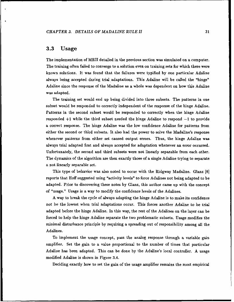
To implement the usage concept, pass the analog response through a variable gain
amplifier. Set the gain to a value proportional to the number of times that particular
Adaline has been adapted. This can be done by the Adaline's local controller. A usage
modified Adaline is shown in Figure 3.4.
Deciding exactly how to set the gain of the usage amplifier remains the most empirical

CHAPTER 3. DETAILS OF MADALINE RULE II 32
r - - - - -------
line controller
input u-. Y- - binary
pattern W output
adjusted1= rsanalog
true + response
analog 4response +
polarityadjuster N
II adjust
MRII Adaline signal
Figure 3.4: An Adaline modified to implement the usage concept.
part of the MRII algorithm. A formula which has worked well in simulations is:
adaptation countgain =1+ M L*MULT * Nr
where N is the number of patterns in the training set and "MULT" is a multiplier value.
Experience indicates MULT = 5 is a good choice. The idea here is to not let the usage
gain get too laxge before the network really gets into a cycle. The next chapter shows some
results of simulations using MRII.

Chapter 4
Simulation Results
This chapter will present the results of using MRII to train various Madaline networks.
Madalines were used to solve several problems including an associative memory problem
and an edge detection problem. An investigation of how well MRIi could train networks to
learn arbitrary input/output mappings was also conducted. This latter investigation also
included a study of the generalizing properties of MRII. Results of these experiments will
be presented following a presentation of the performance measures used to evaluate the
algorithm.
4.1 Performance Measures
To evaluate a learning scheme there needs to be established some set of criteria by which
to measure the performance. Of primary concern is whether the algorithm converges to a
solution. If it converges, how fast does it converge. If it doesn't converge, does it in some
way get close to a solution. In either case it is often desirable to know how well the resulting
trained network responds to inputs that were not in the training set. This is the issue of
generalization. This section will define the measures used to quantify the answers to these
questions.
Before actually addressing the measures used, a few comments on the experimental
technique used for the simulations is in order. The Madaline network begins training with
some set of weight values already set. The simulations randomized these initial weight
values. Each individual weight was selected independently from a distribution that was
uniform on the interval (-1, +1). The training patterns were presented in random order.
33

CHAPTER 4. SIMULATION RESULTS 34
At each new presentation, each pattern was equally likely of being the one presented. The
selection process then was like pulling one pattern out of a grab bag containing all the
patterns and returning the pattern to the bag after each presentation. At regular intervals
during training, all of the patterns would be presented to the network one after another
to check how many of them were being responded to correctly. These "checkpoints" allow
measuring the network's global performance over the entire training set. No adaptations
are performed during these performance checks. If the response to all patterns was correct,
then convergence was said to occur. Finally, the results are presented as the average of
an ensemble of training attempts, each attempt beginning with a new set of randomized
weights.
The first measure to decide upon is one that measures how long it takes the algorithm
to reach a solution. For a Madaline implemented in hardware, the p.ocess of presenting
a pattern and getting a response will take almost no time. If the response is correct the
network can immediately go on to another pattern. If the response is incorrect though,
the network will go through a series of trial adaptations until the output is corrected. The
trial adaptation procedure will take up the majority of the training time. As convergence is
reached, most pattern presentations will require no adaptations. Thus, the reasonable mea-
sure of training time will be the number of pattern presentations that require adaptations
be performed. This will be a good measure of the time an actual hardware implementation
would require for training. Furthermore, the network only learns from its mistakes. A
pattern presentation that requires adaptations be made can be thought of as a learning
opportunity. By measuring network performance against the number of learning opportu-
nities, a measure of the algorithm's efficiency as it proceeds towards convergence can be
obtained.
The Madalines that are of most interest are those with more than one output bit.
Ultimately, convergence will require that all bits of all output patterns be correct. In
measuring performance prior to convergence, one has two choices. One can count the
number of patterns whose bit responses are all correct or one could count the number of
bits that are correct. One would expect that the number of patterns that have a completely
correct response would not increase until almost all the bits are correct. A distinction
will be made then between pattern rates and bit rates. Since the problems which will
be presented later have different size networks and different size training sets, these rates
will be normalized by presenting them as percentages. The learning curves that will be
presented will plot a training rate versus the number of pattern presentations that required

CHAPTER 4. SIMULATION RESULTS 35
adaptations. A -'bit learalg curve" will present the percentage of the total output bits
for the training set that are correct as a function of the number of adaptation causing
presentations. Similarly, pattern learning curves will plot the percentage of patterns whose
response is completely correct versus the learning opportunities.
It is a fact that MRII does not always arrive at a solution. Sometimes it may take a very
long time for a solution to occur from a particular set of initial weights. At other times the
algorithm gets trapped in a limit cycle and will not proceed to a solution. In performing
the simulations in the following sections, the problem to be solved was attempted many
times starting from new initial weights each time. It was necessary to set some arbitrary
limit to the number of patterns requiring adaptation that would be trained on before the
particular attempt was abandoned. If convergence had not occurred by the time this limit
was reached it did not necessarily mean that convergence would not have occurred if training
had continued. This needs to be remembered when a convergence rate is reported. Theconvergence rate represents the number of training attempts that reached a solution within
some limit of training time.
Those training attempts that converge can be used to generate learning curves that
typify the algorithm's performance on that particular problem. What should be done
though for the cases of nonconvergence? For these cases one might want to know how
close to a solution the algorithm came. With some extra circuitry, it would be possible
to build Madalines that could save their weights at intermediate stages during training.
The learning exhibited by MRII is not a monotonic process. This is due to the fact weightchanges are made based only upon the particular pattern being presented rather than
on a global assessment of the effect of weight changes on the entire training set. Someadaptations will cause regression of global performance. With the ability to save weights at
intermediate stages this effect can be minimized. One becomes interested then in the best
performance exhibited at any stage of training. In the cases of nonconvergence, the averagebest performance will be presented as a measure of how close to a solution the network
came.
4.2 An Associative Memory
An associative memory associates an input pattern with an output pattern. A need forsuch an application arose in the adaptive descrambler portion of a translation invariant
pattern recognizer reported in Widrow, et al [11]. The basic structure of the system is

CHAPTER 4. SIMULATION RESULTS 36
shown in Figure 4.1. An retinal image containing a possibly translated figure is presented
to an invariance box. The invariance box outputs a pattern that is unique to the figure
presented and does not change when the figure is translated on the retina. The descrambler
associates this translation invariant representation of the figure with the original figure in a
standard position. The translation invariant input pattern then acts as a key that unlocks
the required desired response. Most associative memories have the ability to perform well
with incomplete keys or keys with errors in them. This was not expected of the application
here. The requirement then is for the descrambler to act as a simple lookup table.
The structure used for this application is a 25 input, 25-feed-25 Madaline. There were36 patterns in the training set. Three different training sets were used, each representing
a different invariance box. The reason for making the descrambler adaptive is because
the exact form of the outputs from the invariance box is dependent on the particular
problem. The intent is to show the ability to associate patterns with different invariant
representations.
The average learning curves for patterns and bits are presented in Figure 4.2. Thepattern learning curve doesn't show an appreciable increase in performance until almost all
the bits are learned. This is because a pattern is not considered correct until all its bits are
correct.
The algorithm always reached convergence when training on this application. It also
reaches a solution in a reasonable amount of training, only needing to adapt on each pattern
about 15 times to insure convergence. The network is not being tasked heavily by this
example. While the capacity of layered feed-forward Madalines is not known, one can
suspect it exceeds 36 for the structure being trained. The example does show that MRII
is capable of training networks with a relatively large number of inputs and units on both
the first and output layers.
4.3 Edge Detector
Image analysis techniques often require extraction of certain features from a scene such
as edges. A Madaline that could be used as a component of an edge detection systemwas simulated and trained using MRII. The problem is illustrated in Figure 4.3. The
Madaline receives its input from a linear array of pixel elements. The array has a horizontal
orientation. It is desired to detect the first "on" pixel scanning from left to right and output
its position by a binary code. The array has eight elements and the case of no pixels being

CHAPTER 4. SIMULATION RESULTS 37
Invariance
BoxRetina
0Q0
Translation
InvariantRepresentation
Adaptive )
Descrambler
Input PatternOutputs in Standard
Position
Figure 4.1: Diagram of a translation invariant pattern recognition system. The adaptivedescrambler associates a translation invariant representation of a figure to its original rep-resentation in standard position.

CHAPTER 4. SIMULATION RESULTS 38
Learning Curve for Patterns for the Associative Memory100
90
S 80-
70
~60-
50
o 403
30
20)
10-
00 100 200 300 400 500 600 700 800
Number of Patterns Adapted On
Learning Curve for Bits for the Associative Memory100
95
90
85
" 80
75
70
f 65
60
55
500 100 200 300 400 500 600 700 800
Number of Patterns Adapted On
Figure 4.2: Learning curves for patterns and bits for the adaptive descrambler associativememory application. Average of training 100 nets. Data points are marked by "o".
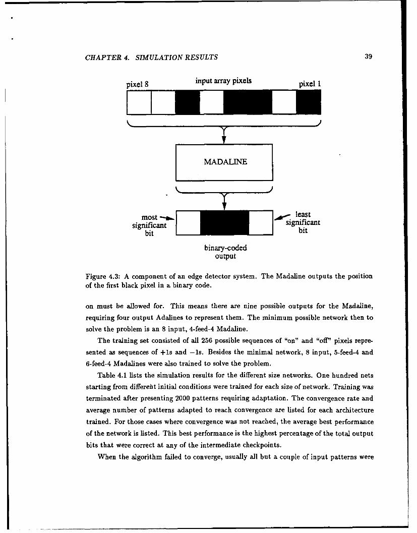
CHAPTER 4. SIMULATION RESULTS 39
pixel 8 input array pixels pixel 1
MADALINE
least
most a sigiiat
significantbit _ bit
binary-codedoutput
Figure 4.3: A component of an edge detector system. The Madaline outputs the positionof the first black pixel in a binary code.
on must be allowed for. This means there are nine possible outputs for the Madaline,
requiring four output Adalines to represent them. The minimum possible network then to
solve the problem is an 8 input, 4-feed-4 Madaline.
The training set consisted of all 256 possible sequences of "on" and "off" pixels repre-
sented as sequences of +ls and -is. Besides the minimal network, 8 input, 5-feed-4 and
6-feed-4 Madalines were also trained to solve the problem.
Table 4.1 lists the simulation results for the different size networks. One hundred nets
starting from differeiit initial conditions were trained for each size of network. Training was
terminated after presenting 2000 patterns requiring adaptation. The convergence rate and
average number of patterns adapted to reach convergence are listed for each architecture
trained. For those cases where convergence was not reached, the average best performance
of the network is listed. This best performance is the highest percentage of the total output
bits that were correct at any of the intermediate checkpoints.
When the algorithm failed to converge, usually all but a couple of input patterns were

CHAPTER 4. SIMULATION RESULTS 40
Edge Detector Performanceave patterns ave best bit rate (M)
network size % convergence adapted to converge for non-converge4-feed-4 52 545 99.5245-feed-4 61 422 99.7756-feed-4 89 282 99.849
Table 4.1: Performance for the edge detector problem. Averages are for training on 100nets beginning at random initial weights.
learned correctly. These unlearned patterns usually only had about one output bit per pat-tern in error. This is why the average best performance for bits even during nonconvergencewas so good. The network had arrived at a solution that satisfied all but a few output bits
out of the 1024 total. This failure to converge lead to an investigation of the algorithm
dynamics to find out why convergence did not occur. The next chapter presents an exam-
ple of a failure mode identified during that investigation. All failures of the algorithm to
converge on this edge detector problem were of this type.
Further examination of the simulation results reveals a not unexpected result. Therewas a noticeable trend as the trained net became larger in size than absolutely necessary to
solve the problem presented. The convergence rate went up and training time, as measured
by the number of patterns adapted to converge, went down.
The use of a network larger than the minimum required will be referred to as "overar-
chitccturing." Overarchitecturing in the case of networks with two layers of adaptive unitsmeans using more first layer units than necessary. The number of output units is fixed
by the problem definition. As one overarchitects, there are more ways to achieve a set of
hidden patterns that are separable in the required ways by each of the output units. This
makes a given problem easier to solve. Thus, it is expected convergence rate would increase
and training required to reach convergence to decrease.
This example problem did not address the issue of generalization. Generalization is theability of a network to respond correctly to patterns it has not been specifically trained
on. In this example, the entire set of possible patterns were presented to the net during
training. The issue of generalization and the effect of overarchitecturing on generalization
performance will be addressed in the next section.

CHAPTER 4. SIMULATION RESULTS 41
Fixed WeightReferenceNetwork
InputPattern
Adaptive I -
~Network
Figure 4.4: Training a network to emulate another. The fixed net provides desired responsesfor the adaptive net.
4.4 The Emulator Problem
One of the intended applications of neural networks is to learn the nonobvious relationships
between the inputs to a decision process and the resulting decision. It is a relatively simple
problem to write down a boolean logic function for the edge detector of the previous section.
Each output bit is a relatively simple function of the eight input bits. The ease with whichthis can be done makes the problem a simple one to program on a computer. In similarfashion one could write logical relationships for each output bit of the associative memory
problem addressed earlier. Due to the dimensionality of that problem, it would not be easy.
Trying to program this problem as a relationship between input bits and output bits wouldbe difficult. Thus, the function the Madaline performs in the associative memory case is
nonobvious. What ability does MRII have to train networks to learn nonobvious, perhaps
arbitrary, input/output relationships?A structure to investigate this question is shown in Figure 4.4. The idea is to train an
adaptive net to emulate a fixed net. The two nets will receive the same inputs and have the
same number of output units. During training, the fixed net acts as a teacher by providing
desired responses to the adaptive net. The fixed net can have its weights set randomly to

CHAPTER 4. SIMULATION RESULTS 42
provide a wide range of arbitrary input/output mappings for the adaptive net to learn. The
adaptive net will have its weights initialized to some other random set of values. MRII will
be used to train the adaptive net to respond just like the fixed net to a given input.
If the adaptive net has the same architecture as the fixed net, then at least one set of
weights exist that will allow the adaptive net to emulate the fixed net perfectly, the set in
the fixed net. With this structure, one can be assured the problem being presented to the
adaptive net is solvable.
The issue of generalization is easily addressed by this structure. Training can be con-
ducted on a subset of the possible input patterns. After training is complete, patterns
not in the training set can be presented in parallel to the fixed and trained nets and their
responses compared.
The issue of overarchitecturing can also be addressed. There is no need for the adaptive
net to have the same number of first-layer units as the fixed net. It could have more. By
zeroing the weights of the unnieded units, the perfect solution offered by the fixed net
could still be obtained. The effect on generalization performance of extra units can be
easily checked.
The example presented here is a 16 input, 3-feed-3 fixed net. Adaptive nets with 3, 6,
and 9 first layer Adalines were trained. Two different size training sets were used. The
smaller set had 650 patterns and the larger set had 1500 patterns. These patterns were
selected randomly from the set of possible input patterns numbering 65,536. Training was
allowed to continue until convergence or 100,000 patterns were adapted upon. After training
was completed, generalization was checked on the balance of the possible input pattern set.
The results are shown in Table 4.2.
As in the case of the edge detector, overarchitecturing improved training performance.
The number of training attempts that reached convergence increased as extra units were
added to the adaptive net. The number of patterns that had to be adapted to reach
convergence decreased as the number of first layer Adalines increased. This is not surprising.
The generalization results though are surprising.
Generalization is seen to decrease with overarchitecturing. This is expected. The
amount of decrease is very slight though and this is surprising. Consider an adaptive
net with nine first layer units versus one with only three. The net with nine units has a
hidden pattern space with 512 patterns available in it. The minimal architecture can solve
the problem with only eight. The fact that the larger net arrives at a solution that preserves
generalization performance is counterintuitive.

CHAPTER 4. SIMULATION RESULTS 43
Emulating a 16 input, 3-feed-3 Fixed Madalineadaptive net convergence ave patterns cnvgd. general. nonconverged bestarchitecture rate adapted bits() Ipats(%) bit trng rate (%)
650 Pattern Training Set3-feed-3 58 1 22940 98.11 95.98 89.286-feed-3 72 20860 96.70 92.20 88.84
9-feed-3 80 16120 95.43 88.66 90.681500 Pattern Training Set
3-feed-3 39 50860 99.20 98.32 92.436-feed-3 65 46610 98.68 96.92 90.339-feed-3 65 37780 98.13 95.36 89.31
Table 4.2: Training and generalization performance for the emulator application. The fixednet was 16 input, 3-feed-3.
As one would expect, the smaller training set is learned quicker and with a greater
convergence rate than the larger set. There is also the expected decrease in generalization
performance. This decrease is slight. This indicates that 650 patterns are sufficient to define
the type of problem the fixed net can present. The 650 patterns are sufficient to insure good
generalization even from the highly overarchitectured 9-feed-3 adaptive net. This training
set represents about one percent of the available patterns in the space.
Use of the smaller training set and larger adaptive nets can save a lot of training time.
The 9-feed-3 net with the smaller training set converges twice as often with one third the
number of adapted patterns as the 3-feed-3 net trained on 1500 patterns. The difference in
generalization performance is modest.
Not all training attempts reached convergence. Table 4.2 reports the average best bit
training rate for those cases that did not converge. Training set size and architecture of the
adaptive net had little effect on this measure of performance. Generalization testing was
performed on these nonconverged cases also. It was found that generalization performance
was very close to the performance on the training set at the cessation of training. To check
how well generalization tracks training performance, a generalization check was done at
each of the training checkpoints. A typical result is plotted in Figure 4.5. The adaptive
network is 9-feed-3, the one with the worst expected generalization performance, being
trained on the 1500 pattern training set. The plot shows that generalization and training
performance track each other closely at all levels of performance. This allows one to expect

CHAPTER 4. SIMULATION RESULTS 44
Training and Generalization Rates During Training100
Training
90-Generalization
80
0U 70
60
Network is 16 input, 9-feed-3
50 emulating 16 input, 3-feed-3
4010 5 10 15 20 25
# of Adapted Patterns (1000s)
Figure 4.5: Tracking of generalization and training performances. Network is a 16 input9-feed-3 emulating a 3-feed-3 fixed net.
that generalization performance will be good anytime one gets good training performance.
The plot shows that little added generalization performance was obtained during the final
9000 adapted patterns that led to final convergence.
The learning curve plot in Figure 4.5 is typical. MRII's performance rises quickly and
then levels off. Further improvements take a relatively long time to occur and do not happen
monotonically.
For those cases of nonconvergence, the final improvement towards convergence did not
happen in the limit set for training time. Unlike the failures to converge identified for
the edge detector and characterized in the next chapter, there is no indication here that
convergence wouldn't occur if enough time were allowed. The failure mode identified in the
next chapter could be responsible but just not recognizable. Due to the larger dimensionality
of this problem, specific reasons for nonconvergence could not be identified.

Chapter 5
A Failure Mode of MRII
The previous chapter showed the MRII algorithm does not always converge to a solution.
Examination of some instances of nonconvergence revealed a failure mode of MRII. This
chapter presents this failure mode by examining a particular instance of it. This particularly
simple example will show that a modification of the algorithm will be required to handle
this mode of failure. Some possible modifications are presented.
A secondary purpose of this chapter is to provide the reader some insight into the
dynamics of the algorithm. The example used in this chapter is simple enough to represent
in two dimensions, allowing presentation using graphical methods. The reader will be able
to see what happens to the mappings from input pattern to hidden pattern to output
pattern as trial adaptations and weight changes are made. While the chapter highlights
a case where the algorithm fails to proceed to a solution, its study can lead to a better
understanding of the methodology used by the algorithm.
5.1 The And/Xor Problem
The particular problem used for this example is called the and/xor problem. The challenge
is to train a 2-input, 2-feed-2 network to give the logical "and" of its inputs as its first
output, and the exclusive-or of its inputs as the second output. The desired input/output
mapping is presented as a truth table in Table 5.1.
A solution for this problem is shown graphically in Figure 5.1. In the figure, the decision
lines of the various Adalines have been identified by the weight vectors which define them.
To allow easy reference to these weight vectors a double superscript is used on the weight
45

CHAPTER 5. A FAILURE MODE OF MRII 46
eq-o 0
--- 7 7
+ +
. ,I* ,
0
Fig 5.1: .- - "
I I +
Figre5.1 Gaphca rersnaino ewr ha ovste0dxrpolm

CHAPTER 5. A FAILURE MODE OF MRII 47
TRUTH TABLEinput desired
pattern responseX1 X2 di d2
+1 +1 +1 -1+1 -1 -1 +1-1 +1 -1 +1-1 -1 -1 -1
Table 5.1: Truth table for the and/xor problem.
vector symbol. For instance, W21 refers to the weight vector of the first Adaline on the
second (output) layer. As there is only one hidden layer in this network, the superscript on
ff and its components has been dropped.
This particular problem forces the Adalines of the first layer to perform double duty.
They must provide a hidden pattern set that can be separated by the second output Ada-
line to do the exclusive-or function. This hidden pattern set must also be separable by
the first output Adaiine to allow realization of the and function. Thus there is an implicit
requirement for the output Adalines to cooperate with each other on settling upon a mu-
tually satisfactory hidden pattern set. The whole goal of MRII is to implement a method
to facilitate this cooperation.
For this particular problem and for some of the problems presented in Chapter 4, there
are states for the network from which MRII cannot proceed to a solution. The next section
will show an example of a limit cycle that MRII cannot escape.
5.2 A Limit Cycle
Consider a network with the following sets of weights in it:
W11 = [.3,-.15, -.3]T
w12 _-[-.15, .05,-.05]T
w'l -[.15, -. 15, .1 5 1T
w2 = [-.15, .15, .15]T

CHAPTER 5. A FAILURE MODE OF MRII 48
State 1input hidden output
pattern pattern patternz1 X2 hi h2 01 02
+1 +1 -1 -1 +1 -1+1 -1 +1 -1 -1 -1"
-1 +1 +1 -1 -1 -1-1 -1 +1 -1 -1 -1
Table 5.2: The input pattern to hidden pattern to output pattern mapping for State 1.Incorrect output responses are marked by *.
These weights were taken from an actual simulation result. They have been rounded to
make easier the algebra and graphing to follow in this section. The decision lines and
mappings for this network are shown graphically in Figure 5.2. The mapping information
is also shown in tabular form in Table 5.2. In the table, incorrect output responses are
indicated by an asterisk. This set of weights and mappings will be referred to as State 1.
The network in State 1 makes an error for two of the four input patterns. The two
patterns produce the same hidden pattern and output response and also have the same
desired response. Therefore, it makes no difference which of these two patterns is considered
first. Until one of these error producing patterns is presented, no adaptations will take place
since the responses for the other two input patterns are correct. When one of the two input
patterns that result in an error is presented to the network, MRII will attempt to correct
the output by trial adapting the first layer Adalines.
At this point, it is important to note that ol is already correct. MRII will then accept
a first-layer trial adaptation only if it completely corrects the output pattern. It will not
accept a "trade" of errors in the bits of the output pattern. The Hamming distance between
the output and desired response must actually be reduced.
For an error producing input, the first layer responds with the hidden pattern hi = +1,
h2 = -1. A trial adaptation can be thought of as moving this hidden pattern to another
position in the hidden space and checking the decisions made by output Adalines on this
new point. This concept is shown graphically in Figure 5.3. This same information is show
in tabular form in Table 5.3. The table shows none of the possible trial adaptations will
completely correct the output so they will all be rejected. Failing to find an acceptable
first-layer adaptation, MRII will proceed by adapting the second output Adaline to provide

CHAPTER 5. A FAILURE MODE OF MRII 49
o 0
-q---+---- ------- -+ + I- 4 I +
/
+
o 0
7 7
F 0a
----------------------------------------------------

CHAPTER 5. A FAILURE MODE OF MDII 50
vV-22 hh 2
o 0o2
flip both / 2
-. h 1
fliph 1
0<
Figure 5.3: Graphical presentation of trial adaptations from State 1.
the desired response, +1, for its input, the hidden pattern hi = +1, h2 = -1.This brings the network to what will be referred to as State 2. The only change in the
network has been to the second output Adaline. The hidden patterns used by the networkhave not changed. It is assumed the response to the hidden pattern hl = -1, h2 = -1,has not been affected. The mapping information for the network in State 2 is shown in
Table 5.4. A repositioning of the second output Adaline's decision line in the hidden space
to provide this mapping is shown in Figure 5.4.
As Table 5.4 shows, the network now makes an error for only one input pattern, xi = -1
and x2 = -1. No adaptations will be made by the network until this pattern is presented.
The possible trial adaptations that can be made in this case will have the same bad resultthat occurred from State 1. All trials will result in ol becoming incorrect. This is because
the hidden pattern is still the same as that considered in State 1 and the decision line of
the first output Adaline has not been changed in getting to State 2. Therefore, all the trialadaptations will be rejected. The second output Adaline will again require adaptation. Its
input is the same as it was when adapting out of State 1, but the error is now opposite to

CHAPTER 5. A FAILURE MODE OF MRII 51
Trial Adapting for State 1Trial Adapt h, h 2 01 02
none +1 -1 -1 -1 *fliph, -1 -1 +1* -1'fliph 2 +1 +1 +1* +1
fipboth -1 +1 +1* -1"
Table 5.3: The results of trial adaptations from State 1.
State 2input hidden output
pattern pattern patternX1 X2 hi h2 Ol 02
+i +1 -1 -1 +1 -1
+1 -i +1 -1 -1 +1-1 +1 +1 -1 -1 +1-1 -1 +1 -1 -1 +1*
Table 5.4: Mapping information for the network in State 2.
what it was. Thus, the adaptation will return the network to State 1, basically undoing
the previous adaptation. The network is in a limit cycle.
The astute reader will now question whether State 2 is the only possible result of
adapting out of State 1. Suppose the second output Adaline's response to the hidden
pattern h, = -1, h2 = -1 had also changed with the adaptation out of State 1. Indeed,
a plausible positioning for the second output Adaline's decision line is shown in Figure 5.5.
This would result in a State 3 whose mapping is detailed in Table 5.5.
An examination of Table 5.5 shows there are now two input patterns that result in
errors. For random presentation order, the pattern x, = +1, x2 = +1 will be presented
prior to the other error producing input sometime State 3 is visited. This input pattern
maps to a different hidden pattern than considered previously. For this hidden pattern, the
trial adaptation involving a flip of h2 corrects the output completely and will be accepted.
This trial adaptation is indicated on Figure 5.5. Thus, there exists a mechanism for escape
from the claimed limit cycle if State 3 can be reached. Unfortunately, State 3 cannot be
reached as a few lines of algebra will now show.
MRII uses the modified relaxation method for performing its weight adaptations. Given

CHAPTER 5. A FAILURE MODE OF MRII 52
V22 h 2
0 cV-21
'] h 1
Figure 5.4: Separation of the hidden pattern space for State 2.
that it is desired to adapt only when there is a binary error present, all of the adaptation
procedures proposed by Mays [3] have the same basic form. Using k as an adaptation
counter, all the weight change formulas have the form,
AVWk = 6 kdkXk, 5k > 0.
Here it is emphasized that the size of the adaptation step is not necessarily constant from
adaptation to adaptation by subscripting 6.MRII adapts only when there is a binary decision error present. This is in accord with
the minimal disturbance principle. When following this procedure, one will note that the
sign of the desired response and the sign of the analog error defined as, Ck = dk - Yk, will
be the same. Thus, even the famous Widrow-Hoff least means squares (LMS) algorithmhas the form above. The LMS algorithm is usually written, AWk = 2tck. Here the
magnitude of 2/1fk can be identified as 5k. All the various weight update methods used
to adapt Adalines differ only in how they choose 6 k. It will be shown that not only canState 3 not be reached, but this non-reachability is not dependent on the weight update

CHAPTER 5. A FAILURE MODE OF MRII 53
-22
0 0 -21
Atrial adaptflip h 2
+
Figure 5.5: An output separation that would give State 3.
rule used.
The situation under consideration is the adaptation of the second output Adaline from
State 1. Assuming k adaptations have occurred to this point, the situation is as follows:j~k +1' -1]T- W22 .5T
= [+1, +1,- 1]T, 02 = -1, d2 = +1, and k = [-.15, .15, .1 5 T, where the bias
input component has been included in the hidden vector. For the moment, generalize theso 22
second Adaline's weight vector to Wk = a[-1, +1, +1]T . This generalized weight vector
implements the same decision line but with a generalized confidence.
The particular requirement is to adapt the second output Adaline to provide a +1
response. Note that if the weight update rule does not select a large enough weight ad-
justment to actually change the binary response of the second Adaline, the network will
remain in State 1. The next presentation of a pattern producing an error will require
further adaptation of the second output Adaline. This will continue until State 2 is finally
reached. The weight update actually used by MRII will put the network in State 2 in one
step. The point here is that there is no advantage to adapting using smaller steps in this
case.

CHAPTER 5. A FAILURE MODE OF MRII 54
Postulated State 3input hidden output
pattern pattern patternX1 X2 hi h 2 O 02
+1 +1 -1 -1 +1 +1*+1 -I +1 -1 -1 +1-1 +1 +1 -1 -1 +1-1 -1 +1 -1 -1 +1*
Table 5.5: Mapping for the postulated State 3.
After reaching State 2, the weight vector for the second output Adaline will have the
form, W,+ = [-a + k, a + k, a - bk]T. A minimum value of 6k can be computed since-T.22
in State 2 it is required, Hk ,+1 > 0. The minimal value of bk works out to be a/3.
For the adaptation from State 1 to result in State 3, another minimal b can be
computed. The requirement to reach State 3 is that the hidden pattern h, = -1, h2 = -1,
be responded to with +1 by the second output Adaline. This requires bk > 3a. Thus, to
reach State 3, an adaptation step nine times larger than that needed to just reach State 2
is required. This fact is independent of the value of a. Such steps may not be consistent with
the minimal disturbance principle. Indeed, they may not be achievable by the particular
weight update rule in use.
Consider what the response to ilk will be if State 3 is reached. This value is what
the adaptation level, L, would have to have been in the MRII weight update rule when
adapting out of State 1. Setting bk = 3a in W*+1 and taking the dot product with I1 k one
gets 8a. For the particular example of this section, a = .15. If State 3 were the result of
adapting from State 1 the resulting response to the adapted on hidden pattern, rik, would
be greater than 1.2.
This resulting confidence is greater than the desired response for this hidden pattern.
None of the weight update rules use step sizes that result in overshooting the desired re-
sponse. Indeed, doing so is certainly not in accord with the minimal disturbance principle.
MRII is based on the minimal disturbance principle. No weight update rule that is consis-
tent with this principle will allow escape from the limit cycle that results in this example.

CHAPTER 5. A FAILURE MODE OF MRII 55
5.3 Discussion
The previous section illustrates an example of MRII caught in a limit cycle. Why did this
cycle happen? The reasons are twofold. First, the first output Adaline reached a solution
before the second output Adaline. Second, the hidden pattern set settled upon by the first
output Adaline was unusable by the second output Adaline in reaching a solution. Any
attempt to change the hidden pattern set by the second output Adaline was .effectively
vetoed by the first output Adaline. Any change to the hidden pattern set destroyed the
solution arrived at by the first output Adaline. Thus, the system had entered a local error
minimum. No change on the first layer could reduce output errors.
The second layer Adalines found themselves in a situation not unlike that which inspired
the usage concept. There existed a nonseparable subset of hidden patterns that the second
output Adaline was forced to try to separate. It was successful at performing the separation
for a given presentation but could not come to a global solution. Unfortunately, usage is
not a technique that can be employed at the output layer. When the output layer is forcedto adapt, there is no freedom left to share responsibility for correcting an output.
At this point it is important to note that usage, even on the first layer, will not solve
this particular example. In examining the possible trial adaptations from State 1, all
were considered and rejected. Usage affects only which particular Adalines participate in
trial adaptations when participation is limited to some number less than the total num-
ber of Adalines on the layer. It can have no effect when all Adalines are considered for
participation.
In this particular example, the limit cycle is easily recognizable. It is characterized
by a lack of accepted trial adaptations on the first layer, and by a single output Adaline
being adapted over and over. The master controller could detect a lack of accepted trial
adaptations. In this case, there is hope for implementing an escape mechanism since a
developed limit cycle can be recognized.
For larger networks with larger training sets, the failure mode may not be so easily
recognizable. It may be possible for output units to come to solutions on subsets of the
training set. These units would then limit the allowable hidden patterns to a small set.
This small set would not allow the other units to come to global solution but allow somefirst-layer trial adaptations to be accepted. The limit cycle would consist of a large number
of specific states. By restricting the hidden patterns to a nonsolvable set, wide variations
of training performance would be seen. This would effectively mask the failure mode. The

CHAPTER 5. A FAILURE MODE OF MRII 56
author conjectures situations like this occurred in some of the failures to converge with the
emulator problem.
Though not reported in the previous chapter, solving the n-bit parity problem was
attempted by MRII. The network required is an n-input, n-feed-1 Madaline. This was
generally successful but a failure mode seen there was quite similar to the one noted above.
The parity problem has a single output, so there is no possibility of another output Adaline
vetoing trial adaptations as in the and/xor problem. What happens instead is that the
allowed trial adaptations are ineffective. The ones tried do not correct the output. This
happens because of the somewhat arbitrary limit placed on the number of Adalines that
will be considered for adaptation. The generally useful heuristic of considering the least
confident half of the Adalines on a layer sometimes fails. In this case, it is easy for the
master controller to increase the number of Adalines considered for adaptation and the
number of Adalines at a time that are trial adapted. Unfortunately, this procedure is very
heuristic. It does however work. With some experience, methods using this concept can be
implemented to cause the n-bit parity problem to almost always converge. The fine tuning
used to achieve good convergence for the n-bit parity problem will not always transfer to
another problem, nor even to the (n + 2)-bit parity problem so the details are omitted here.
Sometimes with smaller nets, all possible trial adaptations would be tried and rejected.
The cause for this was a large bias weight being initialized in the ouput Adaline. The bias
determined the network's response and the first-layer Adalines weren't weighted sufficiently
to have any effect. A simple solution to this is to initialize the weights in the output Adaline
all equal. It then starts as a majority voter, giving every first layer Adaline equal say in the
network response. In any event, these techniques will not allow escape from the and/xor
limit cycle detailed above.
The specific and/xor example cited in this chapter resulted after several earlier adap-
tations. Starting with the same initial weights, a different pattern presentation sequence
would avoid the limit cycle and instead converge to a solution quite quickly. The point is,
there seems to be no way to characterize a set of initial weights as being a set that leads to
a limit cycle. Indeed, a cursory look at the weights that were presented at the beginning
of the chapter shows nothing remarkable about them. They could easily have occurred at
initialization. Indeed, weights that define a limit cycle condition sometimes do occur at
initialization. It seems unlikely that a method for avoiding limit cycles can be found while
retaining the basic form of the algorithm. The only feasible strategy seems to be to detect
the limit cycle and then implement some escape.

CHAPTER 5. A FAILURE MODE OF MRII 57
The minimal disturbance principle underlies the MRII algorithm. Any limit cycle escape
mechanism will have to selectively depart from the minimal disturbance principle, perhaps
in an extreme fashion. The size of the adaptation level needed to reach State 3 is an
example of how extreme this departure may have to be.
Various techniques have been used with varying degrees of success. Most are of a
heuristic nature, and often need to be hand crafted for the particular problem being solved.
Some of these techniques include: allowing the adaptation level of non-output units to
be a random variable; modifying the output unit adaptation levels by their usage count;
modifying the number of Adalines allowed to participate in trial adaptations by the average
output unit usage count. None of these offer much hope of being generally applicable.
Probably the easiest escape that is generally applicable is to reinitialize the weights in
the system and start the training over. Often this is not a bad thing to do. Experience
indicates that if MRII is going to find a solution it will find it fairly quickly. If training
performance levels off at an unacceptable level, after a reasonable time, start over. The
determination of a reasonable time can be done by doing an ensemble of training attempts.
A look at the average learning curve will reveal an average performance increase versus
adaptations performed. This will allow extrapolation to the convergence point allowing
one to set a reasonable limit to the number of adaptations that will be performed before
reinitializing.
Reinitialization has the drawback of losing all benefit of training performed up to that
point. Often the system will be somewhere near a solution and merely needs nudged out
of a local minima. One way to do this is to occasionally add some random perturbations
to the weights. This moves the system to a random place in weight space. The idea is to
get away from the local minima but not so far away from the previous weight position as
to negate all previous train" ig.
It is hoped this weight perturbation method would have some generality to it. Some
preliminary success has been achieved using this technique with the n-bit parity problem
for n up to seven. The perturbation magnitude needed and a schedule for applying it were
determined by experience. The magnitude of perturbations needed for a general problem
might depend only on the particular architecture being trained. Thus, an analysis of the
effect of weight perturbations on the input/output mapping of a Madaline system might be
very helpful in generalizing this technique. This reasoning is the prime motivation for the
sensitivity work presented in the next chapter.

Chapter 6
Sensitivity of Madalines to Weight
Disturbances
6.1 Motivation
It's been shown the training performance of Madaline Rule II rises quickly and then levels
off. For even moderately sized networks, the number of training attempts that result in
convergence represent a smaller fraction of the total attempts than one would like. For some
architectures, considerable refinement of the number of Adalines allowed to participate in
trial adaptations and adjustment of the "MULT" factor of the usage gain is required to get
performance levels like those reported in Chapter 4. The identified failure mode presented
in the previous chapter may account for much of the problem. In larger networks this failure
mode may be difficult to recognize. However, the problem may be more fundamental.
For the emulator problem, the weights in the fixed net were generated randomly. It may
be the network is non-robust in the weights. The mapping from input patterns to outputs
may change significantly for a very small change in the weights of the fixed net. If such
is the case, how close do the weights in the trained adaptive net have to be to the perfect
solution weights of the fixed net to get good performance? What is the rate of performance
degradation as the weights deviate further and further from exactly right?
An investigation of the sensitivity of the input/output mapping to changes in the weights
may lead to insightful improvements of the MRII algorithm. It was proposed at the end of
the last chapter to use random weight perturbations to escape from the algorithm's failure
mode. A thoughtful approach to this method requires some understanding of the weight
58

CHAPTER 6. SENSITIVITY OF MADALINES TO WEIGHT DISTURBANCES 59
Madalinewith
reference weights+
input r w errorpattern p ve
MadalineL--6-withperturb.r weights
Figure 6.1: Comparing a network with a weights perturbed version of itself.
sensitivity issue. The study may also suggest modifications of the network architectures
and input representations to minimize the effects of weight disturbances.
The investigation uses a structure similar to that of Figure 4.4. Instead of an adaptive
network being compared to a fixed network, a perturbed v hesion of a net is compared
against the unperturbed net, called the reference net, as shown in Figure 6.1. The effect
of weight changes, with known statistical distribution, on the input/output mapping of asingle Adaline is done first.
6.2 Perturbing the Weights of a Single Adaline
Hoff [6] did an analysis of the effect of weight perturbations on the decision mapping of
an Adaline using the hypersphere approximation. He did his analysis in the n-dimensional
pattern space. As pointed out in Chapter 2, the bias weight introduces a complication
to such an analysis. The bias weight is not considered part of the weight vector by Hoff.
This causes the separating hyperplane to pass through the pattern hypersphere offset from
the origin by a distance dependent on the bias weight, and the magnitude of the reduced
dimension weight vector. Changes in the weights must then be resolved into components
parallel and perpendicular to the weight vector. The final results were complicated and
difficult to apply to answering the question of how close weights have to be to a known
solution for good performance.

CHAPTER 6. SENSITIVITY OF MADALINES TO WEIGHT DISTURBANCES 60
By using the hypersphere approximation in the (n + 1)-dimensional weight space, sim-
plifications occur. The input pattern is now considered to be of dimension n + 1, but with
the bias input, xo, a constant +1. The set of all possible input patterns now lie on the
positive x0 half of a hypersphere of radius V'WWT centered at the origin of (n + 1)-space.
Glanz [8I maintained the hypersphere approximation could now be applied to this hemi-
hypersphere. The patterns are now confined to an oriented half of the hypersphere but
within this region they are assumed uniformly distributed. The major simplification is that
now the separating hyperplane always passes through the origin. The decision of which
input patterns are classified +1 and which are -1 is determined by how the hyperplane
intersects the pattern hemihypersphere. Changes in the weights cause the orientation of
the hyperplane to change. These changes can now be described by a single parameter, the
angle between the original weight vector and the new weight vector.
In Figure 6.2 the positive x0 hemihypersphere, a weight vector, a perturbed weight
vector and the associated intersections of the decision hyperplanes are shown. The result
of perturbing the weight vector is a reorientation of the decision hyperplane. For those
patterns in the darker shaded region, the perturbed network will make a "decision error"
relative to the reference network.
The darker shaded area consists of two partial lunes. By symmetry, one can see the
area of the two partial lunes add to that of a lune of angle 0, the angle between the weight
and perturbed weight vectors. Using the hypersphere approximation, the probability of a
decision error due to a shift in the weight vector is:
P[Decision Error] = Area of shaded luneArea of hemihypersphere
0
7r
Taking the expectation of both sides,
Ave P[Decision Errors] = E _} (6.1)7r 7r
To determine j, look at Figure 6.3. In (n + 1)-space, V and AW determine a plane and
the angle between them in that plane, 0. The angle, 0, between W and W + AW can be
found by plane geometry.
0 = tan-1 IJA'WIsin0 = tn JIl + IAN~vl cos i,

CHAPTER 6. SENSITIVITY OF MADALINES TO WEIGHT DISTURBANCES 61
ZO
hemihypersphere
00
decision decisionhyperplane hylerplane for
for W Vv" +/A7
Figure 6.2: Reorientation of the decision hyperplane due to a disturbance of the weightvector. Patterns lying in the darker shaded region change classification.
I sin= tan-1
- l + cos€FxWI
tan- 1 (J W sin j for IWI > 1
Using tan - 1 x x for small x,
9 A"W I sin
Then,
'W i
It has been assumed here that the ratio of the magnitude of the weight perturbation vectorto the magnitude of the original weight vector is known and constant. If this is not the

CHAPTER 6. SENSITIVITY OF MADALINES TO WEIGHT DISTURBANCES 62
%\IzAVI sino
IAxW cos o
Figure 6.3: Geometry in the plane determined by W and AW.
case, but the perturbations are independent of each other and independent of the original
weights, an average perturbation magnitude can be used.
To complete the derivation of the average decision errors a single Adaline makes due
to perturbation of its weights, a formula for E{sin 0} is needed. The vectors WV and ALV,
or their extensions, will intersect a hypersphere of unit radius. Since only the directions
of these vectors determine 0, the analysis can assume a unit radius sphere without loss
of generality. Glanz [81 notes that the probability that the angle between two vectors, V,
and V2, has value between 0 and 0 + A0 is proportional to the differential area at angle 0
(see Equation 2.4). Modifying his equation for use in (n + 1)-space, the probability density
function can be written,
p[ Vi and V2 form angle ] = sin+--' (6.2)
Therefore,
E{sin0} fir sin J Kn sin'-'d<0 Kn+ I
2K,. I 2-sinn~s
Kn(nllo
2K, V r(nl)
Kn+ 1 2F(1 + 1)

CHAPTER 6. SENSITIVITY OF MADALINES TO WEIGHT DISTURBANCES 63
- r(+) 2r+ r( + 1)
r2 (n2) 2r () n
(_KLn) 2 27r (6.3)
This result can be further simplified by using Stirling's approximation for factorials and
the expressions for Kn for n even and odd in Equations 2.2 and 2.3. Stirling's approximation
is:
n! ; V2"nnne-".
For n - 2m,
Kn 27r' (2m)!
Kn+1 (m - 1)! 7rm2 2m+1m!
(2m)!22- M! (M- )
m (2m)!
22m (M!) 2
mv'4"rm (2m)2me- 2m
22m 27rm M 2me - 2m
ffT = for n even.
Fornodd, n =2m+l and n+ 1 =2(m+l),
Kn _ '22- +l(M)! mn!
Kn+j (2m)! 27rm+l
22m (M!) 2
ir (2m)!
2 2m (v2- me-m )
irV - 2 (2m)2me-2m
2irm
n- for n odd.
V•m mm2m

CHAPTER 6. SENSITIVITY OF MADALINES TO WEIGHT DISTURBANCES 64
For n sufficiently large, the even and odd cases become indistinguishable and it can be
approximated,
T for n large (6.4)Kn+l 7
With this result, Equation 6.3 becomes,
E{sin 0} ;7r)n
S1 for n large
The final result for determining the change in the input/output mapping of an Adaline
caused by a disturbance of its weights can now be formulated. Using the results so far,
P[Decision Error] = 37r
l -tVW 2 r (6.5)7r I I Kn+1 ) n
S1 (6.6)
The last two expressions represent different levels of approximation. Future reference will
call the first the complicated approximation while the second will be called the simple
approximation. The simple approximation ignores any dependency on the number of inputs
and is good in the limit as n gets large.
6.3 Decision Errors Due to Input Errors
The above result can be used to predict the error rate of an Adaline in the first layer of a
multilayer network. For a randomly generated reference network, it can be assumed that
first-layer Adalines will behave independently of each other. Assume all Adalines of the
first layer are affected by weight disturbances such that their weight perturbation ratios,
JAW/IWI are the same. They will all have, on average, the same probability of making an
error. The number of errors in the output of this first layer of a perturbed network relative
to the reference network will be binomially distributed. This distribution has as parameters
the number of first-layer Adalines and the error rate of an Adaline.
The perturbed net's second layer will see inputs that are in error relative to those seen
by the second layer of the reference network. Some of these erroneous patterns may cause

CHAPTER 6. SENSITIVITY OF MADALINES TO WEIGHT DISTURBANCES 65
decision errors at the network output even if there are no weight errors in the second and
subsequent layers. The basic question to investigate then is, how do random input errors
affect an Adaline's decision mapping?
In the binary case where the components of the input are either +1 or -1, an input
error can be thought of as a "flipped" bit. If a pattern has one flipped bit, the result is a
nearest neighbor, a pattern of Hamming distance one from the original. One way to think
of flipping a bit is to add a AR to R. To generate a nearest neighbor of X, add a vector to
it that has all components equal to zero except for one, say the ith. Let the ith component,Axi be equal to -2xi. This disturbance vector has a Euclidean length of two.
In general, you can generate a pattern vector which is a Hamming distance h from a
given pattern A, by flipping h of its bits. This can be done by adding a disturbance vector
AX having h nonzero components equal to -2 times the corresponding X component. This
AR will have a Euclidean length of vA4-h.
Note that all of 's pattern neighbors of Hamming distance h are at the same Eu-
clidean distance from R. Thus, the pattern neighbors of given Hamming distance from 9lie on a hypersphere of radius /4h with the tip of 9 as origin. The neighbors also lie on
the pattern hemihypersphere on which X is located, since they are legitimate patterns in
the input space. The possibility of the bias input being flipped is excluded. The inter-
section of these two hyperspheric regions is a hypersphere of dimension one less than the
pattern hemihypersphere. Hoff's hypersphere approximation leads one to conjecture that
the pattern neighbors of YC are uniformly distributed on this reduced dimension surface.
A visualization that supports this conjecture is shown in Figure 6.4. Consider the situa-tion where n = 3 and there is no bias input. The eight patterns available in 3-space form
the vertices of a cube which can be inscribed in a sphere (not shown in the figure). The
vertex marked )9 has three nearest neighbors. They lie equally spaced on a circle which
lies in a plane. Furthermore, the vector 9 intersects this plane at the center of the circle.
For the following analysis, it will be assumed the conjecture of a pattern's neighbors being
uniformly distributed in the reduced dimension space to be true.
If the weight vector components are chosen from a zero mean distribution, the weight
vector will be orthogonal to the xo axis, on average. This is because the expected value
of the dot product of the weight vector with the x0 axis is the expected value of the biasweight, which is zero. This leads to the intuitive conclusion that an "average" Adaline will
have equally likely +1 and -1 outputs. This average Adaline will be analyzed to determine
the effect of random input errors on its input/output map.

CHAPTER 6. SENSITIVITY OF MADALINES TO WEIGHT DISTURBANCES 66
nearest . tn~ghbor"
nearest neighbor
Figure 6.4: The nearest neighbors of X lie equally spaced on a reduced dimension hyper-
sphere.
The idea of the analysis is shown in Figure 6.5. Without loss of generality, assume the
pattern vector of interest lies on the positive side of the decision hyperplane. Shown
in the figure is a representation of the location of the pattern neighbors located Eucidean
distance d from two different X s. Xi is located sufficiently far from the decision hyperplane
that all of its pattern neighbors distance d away will be classified positive. No errors will
be made by this Adaline if any of these neighbors are input instead of the correct pattern
. The pattern 2 is located closer to the decision hyperplane and some of its neighbors
at distance d are on the opposite side of the decision hyperplane. Thus, a fraction of those
times that a neighbor is presented instead of the correct cl2, a decision error will be made
by the Adaline. It will be determined here what fraction of these neighbor presentations
will result in decision errors.
At this point, the notions of dimensionality need to be made more precise. The termi-nology employed by Sommerville (101 will be used. The input patterns lie on a hypersphere

CHAPTER 6. SENSITIVITY OF MADALINES TO WEIGHT DISTURBANCES 67
pattern o
hemihypersphe,"
-------- X2o"d
_...-_decision
Figure 6.5: All the patterns at distance d from I will be classified the same as X1. Someof the patterns at distance d from ,2 are classified different from 92.
of n dimensions in (n + 1)-space. The hypersphere is of dimension n because only n compo-
nents are needed to specify a point on this surface. The 2'n patterns considered to make up
the input space of the Adaline are confined to the positive x0 hemihypersphere. The bias
input is supplied internally by the Adaline and is considered not subject to error. As has
been pointed out before, the decision hyperplane of an Adaline described analytically by
XT v = 0, is a surface of n dimensions. Sommerville calls this an n-fiat but will be referred
to as an n-dimensional hyperplane here. The pattern neighbors of 9 at Euclidean distance
d are located on a surface defined by the intersection of two hyperspheres of n dimensions
in (n + 1)-space. The first hypersphere is the one of radius ,/W-+ centered at the origin
and the second is the hypersphere of radius d = V/7 centered about the tip of 9. This
intersection is a hypersphere of dimension n - 1. Furthermore, this intersection lies in an
n-dimensional hyperplane. This can be seen as follows. Let I4 be a pattern neighbor. It is
representable by 1q = , + A9 where A9 is of the form described earlier. Then,
= = II z +

CHAPTER 6. SENSITIVITY OF MADALINES TO WEIGHT DISTURBANCES 68
v Xneighbor
os
Figure 6.6: A representation of the location of the patterns at distance d from the inputvector .
= n + 1 + -2h = a constant,
h being the Hamming distance of the neighbor. This is the equation of an n-dimensional
hyperplane at a distance from the origin of (n + 1 - 2h)/iF F1 = r - (2h/r) where
r = /n-+ 1 is the radius of the pattern hypersphere. Thus, the pattern neighbors of )9
at Euclidean distance d lie on a hypersphere of limension n - 1 which is contained in an
n-dimensional hyperplane.
The details of the geometric analysis are presented in Figures 6.6-6.8. Figure 6.6 shows
a representation of the situation in the (n + 1)-dimensional pattern/weight space. Here
the perspective is rotated such that the true pattern vector Y. is pointing up. The pattern
neighbors of ) that lie at Euclidean distance d from X are represented by a circle which lies
on the pattern sphere. This circle lies in a plane which cuts off a spherical cap. This cap is
shaded in the figure to aid visualization. The figure is only an aid for visualization purposes.
More precisely, the patterns are located on a hypersphere of n dimensions. The pattern
neighbors are on a hypersphere of n - 1 dimensions which lies in an n-fiat which cuts off a
hyperspherical cap from the pattcrn hypersphere. Because the perspective has been rotated,
the hemisphere shown in the figure no longer represents the pattern hemihypersphere. The

CHAPTER 6. SENSITIVITY OF MADALINES TO WEIGHT DISTURBANCES 69
decision
hypersphere
Figure 6.7: A representation of the geometry in the plane formed by W and .
pattern neighbors of 9 do lie on the pattern hemihypersphere, however, and it will be
assumed that their distribution is unaffected by "edge" effects caused by the actual position
of the pattern hemihypersphere. This assumption is good for the average Adaline that has
not too many input errors in the pattern presented.
The pattern vector A and weight vector W define a plane. Figure 6.7 shows the geometry
in this plane. This plane intersects the decision hyperplane in a line, and the pattern
hypersphere in a circular arc. The plane intersects the hypersphere of n - 1 dimensions
containing the pattern neighbors in two points. Ordinary plane geometry can be used for
analysis in this plane formed by X and W.
A representation of the hyperplane containing the pattern neighbors is shown in Fig-
ure 6.8. This hyperplane forms the floor of the hyperspherical cap, and the circle represents
the hypersphere in which the pattern neighbors lie. The center of this hypersphere is the
intersection of the hyperplane containing the neighbor patterns and the vector ). The deci-sion hyperplane intersects the hyperplane containing the pattern neighbors in a hyperplane
of dimension n - 1 or an (n - 1)-flat, represented by a line in the figure. The pattern neigh-
bors on the opposite side of the decision hyperplane from the center of the pattern neighbor
hypersphere will cause errors if they are presented to the Adaline instead of the true pattern
A. The Hoff hypersphere approximation says the probability of error will be the ratio of
the area of the neighbor hypersphere on the opposite side of the decision hyperplane to the
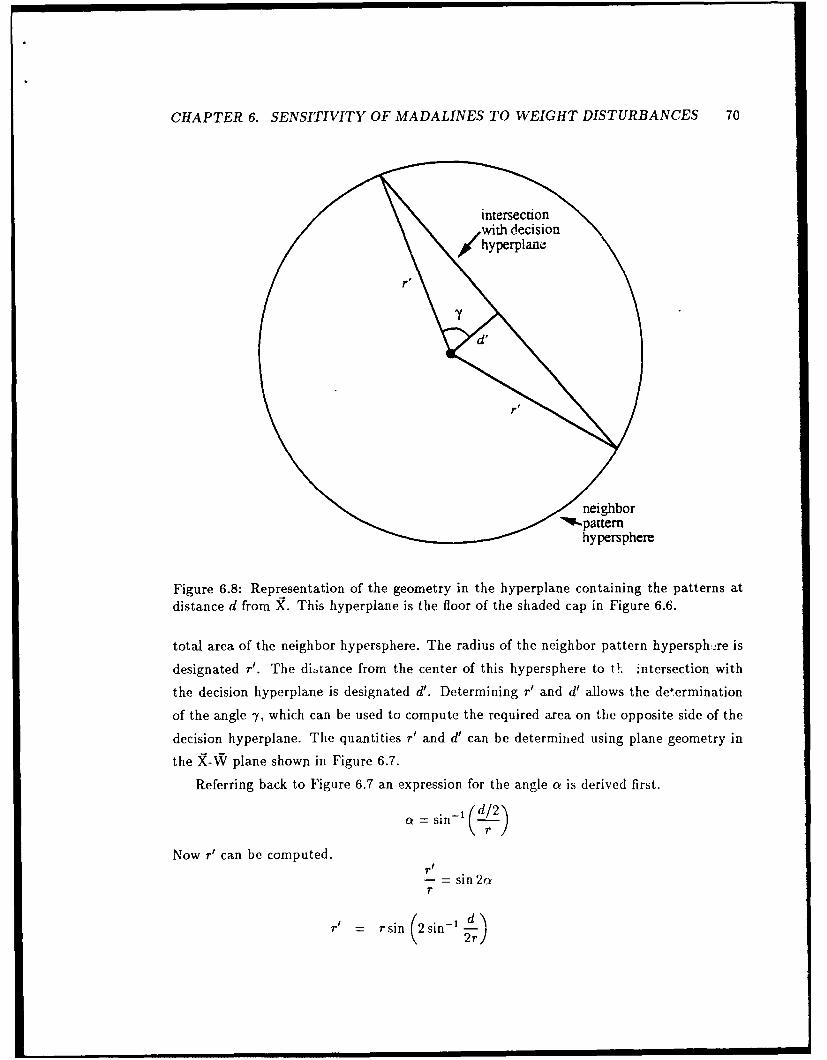
CHAPTER 6. SENSITIVITY OF MADALINES TO WEIGHT DISTURBANCES 70
intersection
hypersphere
Figure 6.8: Representation of the geometry in the hyperplane containing the patterns at
distance d from X. This hyperplane is the floor of the shaded cap in Figure 6.6.
total area of the neighbor hypersphere. The radius of the neighbor pattern hypersphre is
designated r'. The ditance from the center of this hypersphere to ts :ntersection with
the decision hyperplane is designated d'. Determining r' and d' allows the determination
of the angle y, which can be used to compute the required area on the opposite side of the
decision hyperplane. The quantities r' and d' can be determined using plane geometry in
the I9-W plane showni in Figure 6.7.
Referring back to Figure 6.7 an expression for the angle a is derived first.
Q= sin-1 (-d)
Now r' can be computed.r
i
- = sin 2ar
r/ = r sin(2 sin 1 d
.. • miramm u nlmmlmn IiI1 |2r)

CHAPTER 6. SENSITIVITY OF MADALINES TO WEIGHT DISTURBANCES 71
= 2rsin (sin- d) cos (sin- d )
= 2r± 1 - d)"
= d - r
An intermediate result, s is now derived.
S- = Cos 2ar
3 = rcos(2 sin-1 d)
= r (1-2sin2 (sin- dr))
2r2 - d2
2r
With an expression for s, d' can now be derived.
d l- = tan/3S
d 2r2 - d22r
Now -f can be derived by referring to Figure 6.8.
y =I= Cos- I (22-" _ a
- ~ 2 cosj ((r~ 7dr )2)
= C ((2r2-d2) tan,)
- os- \ -r_ -( 6.
= cos - (p t a n ) (6.7)

CHAPTER 6. SENSITIVITY OF MADALINES TO WEIGHT DISTURBANCES 72
where p is defined,p = 2r 2 - d2 (6.8)
The area of the neighbor hypersphere on the opposite side of the decision hyperplane
from the true input vector can be expressed by the integral,
0 r Kn-1 (r i sin O),n-2 r'dO.
This integral sums up slices perpendicular to the line that d' lies on in Figure 6.8. Each
slice is the area of a hypersphere of dimension n - 2, and has a thickness of r' d4, where 0 is
an angle measured from the line d' lies on. The probability of error then when a neighbor
pattern is presented instead of the true pattern is the ratio of the integral above to the total
surface content of the neighbor pattern hypersphere,
P[errorlinput error] = E_ jcos-,W) sin n- 2 dO (6.9)
This conditional probability is a function of 3, the angle from X to the decision hyperplane.
For,3 ; 0, the pattern R lies very close to the decision hyperplane and one would expect the
probability of an error to be one-half. Indeed, the reader can check that Equation 6.9 yields
a value of one-half for 0 = 0. For /3 > 2a, X is sufficiently far from the decision hyperplane
that none of the pattern neighbors produce errors. To get an average probability of error
when the input is a pattern at distance d from the true input, the error rate above must be
weighted by the probability density of finding the true pattern at angle /3 from the decision
hyperplane. For positive patterns, /3 is 7r/2 less the angle between 9 and W. Using a
modification of Equation 6.2 and remembering the patterns exist on a hemihypersphere,
the average probability of error for an average Adaline can be written,fo2cC'(P) Kn- sin d.. __ o do
Ave P[decision error] = 11Ksin" 2 ,d) cos 1/3 d/310 0Kn, IKn+l1
K. 2 sin-1 d. (PP
2 -I 21 / sinn-20cos'-/d' d/3 (6.10)
This double integral can be evaluated numerically on a computer. Because of the de-
pendency of the upper limit of the inner integral on the outer variable of integration and
the large range of integration of the inner integral, it is difficult to arrive at a closed form
approximation. An approximation arrived at by a combination of intuition and accident is,
1 I XlAve P[decision ec ror] - . (6.11)

CHAPTER 6. SENSITIVITY OF MADALINES TO WEIGHT DISTURBANCES 73
This approximation is quite similar to the result obtained when decision errors due to
weight errors were analyzed. The intuition was that there exists a basic symmetry when
working in the (n + 1)-dimensional pattern/weight space. No further justification of the
approximation will be presented other than to show during the results to follow that it is
accurate. The approximation is most accurate for small numbers of errors in the patterns
but is not unusable for numbers of errors approaching half the number of inputs. The
integral expression cannot be expected to hold for errors numbering more than this due
to the assumption about "edge effects" not affecting the distribution of neighbor patterns
about the true pattern.
At this point it should be noted that though the effects of weight errors and input errors
are similar, their effects are independent. The above result for input errors is unaffected
by weight errors that might be present. The result shows the effect of using a pattern's
neighbors at a given distance away from it as inputs to the Adaline instead of the pattern
itself. When looking over the entire input space, it really doesn't matter where the decision
hyperplane is (as long as the Adaline is close to average). For a particular position of the
decision hyperplane, there will be a set of patterns whose neighbors will cause errors if
the neighbors are presented. Moving the position of the hyperplane by weight errors will
change that set of patterns which will be involved in decision errors if their neighbors are
presented, but over the input space, the number of such patterns will remain the same.
Therefore, if errors in the weights are also present, these errors will, on average, affect only
those patterns which are presented with no input errors.
6.4 Total Decision Errors for Adalines and Madalines
The results from the above two sections now allow a formulation of the total probability of
an Adaline making a decision error due to the combined effects of weight errors and input
errors. In networks where it can be assumed the Adalines are independent of each other,
this result can be extended to predict the error rate of the entire network.
An introduction of new notation will facilitate writing the results compactly. Define
Vh as the probability an Adaline makes a decision error given that its input has h errors.
Define . as the total probability that an Adaline makes a decision error. Then,
E = Zh P[input has h errors] (6.12)h=O

CHAPTER 6. SENSITIVITY OF MADALINES TO WEIGHT DISTURBANCES 74
From Section 6.2 and the discussion above about the independence of weight errors and
input errors it is concluded that,
DO r K_ - (6.13)r I V Il ,+
A(6.14)
Dh for h other than zero is obtained from Equation 6.10 or 6.11. At this point use the
facts that r = / +I and d = V47h in these two equations and the defining equation for p.
As explicit functions of h and n they become,
p2
si- o 0
Ph = 2 Kn-: ' J0 sinn-2€ cosn-13 dod/o (6.15)
1 4hV n+1(6.16)
and p as defined in Equation 6.8 is now given by,
n + 1 - 2h
The equations above allow one to predict the average decision errors that a weights per-turbed Madaline will make relative to its unperturbed reference. The use of Equations 6.13
and 6.15 in Equation 6.12 will be referred to as the complicated approximation. The sim-
ple approximation will mean the use of the simpler Equations 6.1A and 6.16. Knowledgeabout the relative magnitudes of the weight disturbance vectors relative to the unperturbed
weight vectors of the Madaline is needed.
When comparing a perturbed net against a reference, one must assume the input pat-
terns to the first layer contain no errors. The reference will respond to what it sees as if itwere the true input and the perturbed net's response is compared against the reference's
output. The theory developed above however is more powerful. It can be used to factor in
knowledge about the distribution of errors in the input patterns to a network to predict its
performance under real conditions.
An analysis begins with the first layer. If only weight errors are present, Equation 6.13
or 6.14 will provide the error rate for each Adaline on the layer. The binomial distribution
is used to predict the probability of the first hidden pattern having a given number of errors.

CHAPTER 6. SENSITIVITY OF MADALINES TO WEIGHT DISTURBANCES 75
This then is the input error distribution for the second layer Adalines. This information is
used in Equation 6.12 to predict the error rate for each Adaline in the next layer, etc.
The above derivations made use of some approximations. Most of these approximations
required either the weight perturbations or the Hamming distance between true inputs and
erroneous inputs to be small. The results, especially Equations 6.14 and 6.!6 are quite
simple in form. They cannot be expected to hold in cases of large weight perturbations or
high probability of input errors. The next section will show the results of simulations to
check the accuracy of the theory and the approximations of the theory made above.
6.5 Simulation Results
The system depicted in Figure 6.1 was used to test the theory developed in the previoussections. A reference Madaline system was generated randomly by selecting each weight
in the system independently from a uniform distribution over the interval (-1, +1). Theseweights were then copied to the perturbed system.
To the weight vectors of each Adaline in the perturbed system a weight perturbation vec-
tor A was added. This vector was generated by selecting each component independently
from the same uniform distribution as before. The perturbation vector was then scaled so
that a desired weight perturbation ratio, jAWjIiWV, was obtained. Thus the assumptionsof the derivation were maintained. The orientation of the perturbation weight vector was
random and independent of the reference weight vector but had a fixed magnitude relative
to the reference. This weight perturbation ratio is expressed as a percentage in the results
that follow.
A large number of patterns from the input space were then presented to the reference and
perturbed systems in parallel and their outputs compared. If any bit of the outputs differed,
a decision error was said to have been made. The results present the number of decision
errors as a percentage of the patterns tested. For any given architecture being checked,this procedure was repeated for several different reference systems. Several perturbations
of each reference system were tested. The results presented are the average percent decision
errors over the different references and their perturbations.
The first system investigated is that of a single Adaline. No input errors are allowed
since the reference needs a true input to calculate a true result. The only term needed inEquation 6.12 then is the DO term. The simulation performed used fifty reference Adalines.
Each reference was compared with fifty different perturbations of itself and the results

CHAPTER 6. SENSITIVITY OF MADALINES TO WEIGHT DISTURBANCES 76
Single Adaline Sensitivity Study% Decision % Decision % Decision
kziwI Errors Errors Errors
(V % Simple Complicated SimulationApproximation Approximation Results
5 1.59 1.50 1.5310 3.18 2.99 3.1120 6.37 5.98 6.1530 9.55 8.97 9.06
n= 165 1.59 1.54 1.56
10 3.18 3.09 3.1220 6.37 6.17 6.1930 9.55 9.26 9.17
n =305 1.59 1.57 1.57
10 3.18 3.13 3.1420 6.37 6.26 6.2430 9.55 9.39 9.22
n =49
5 1.59 1.58 1.5810 3.18 3.15 3.1620 6.37 6.30 6.2530 9.55 9.45 9.24
Table 6.1: Effects of perturbing the weights of a single Adaline. The predicted and simulatedpercentage decision errors for weight disturbance ratios of 5, 10, 20 and 30 percent are shownfor Adalines with 8, 16, 30, and 49 inputs.
averaged. This was repeated at each value of weight perturbation ratio. The predictions
by the simple and complicated theory approximations and the simulation averages are
tabulated for different n and IA'7I/IWl in Table 6.1.
The results show there is a weak dependence on n which is well predicted by the com-
plicated theory approximation. The simple approximation is good in the limit as n grows
large and is an upper limit. The simulation results generally lie between the predictions of
the two formulas. To gain an appreciation of the weak dependence on n and how close the
simple approximation is, the data and the simple approximation prediction are plotted in

CHAPTER 6. SENSITIVITY OF MADALINES TO WEIGHT DISTURBANCES 77
Single Adaline Sensitivity Study10
9-
.:.
7-
o 4-
g' 3
2 Simple Approx....... Simulation for
1 n 8,16,30,49
0 5 10 15 20 25 30
Percent Weight Perturbation Ratio, - *- • 100%
Figure 6.9: Sensitivity of the single Adaline. Dotted lines are simulation results for Adalineswith 8, 16, 30, and 49 inputs. Solid line is the theory prediction by the simple approximation.Data is taken from Table 6.1.
Figure 6.9. The plots nearly lie on top of each other. The complicated approximation would
lie on top of the simulation plots and is not shown. The important thing to note is the
linear dependence on the weight perturbation ratio as predicted by the theory is borne out
by the simulation results. It can be concluded that the theory is very accurate in predicting
the effects of weight perturbations on a single Adaline.
For a network with randomly generated weights, the above validated theory can be
applied independently to each Adaline in Lhe first layer. The distribution of the Hamming
distances between the hidden patterns of a reference and perturbed system can be predicted
using the binomial distribution. This information can be used in Equation 6.12 along with
the results derived for the effect of input errors on the decision mapping of an Adaline
to predict the performance of second (output) layer Adalines. As before, the simple and
complicated theory approximations will be presented.

CHAPTER 6. SENSITIVITY OF MADALINES TO WEIGHT DISTURBANCES 78
Input Errors and Decision Errors for Output Adaline49 input, 35-feed-1 Madaline, W = .2
frequency (%) of input errors miss rate, Dh (%), of each input errorerrors simple complicated observed simple complicated observed
0 10.00 10.25 10.47 6.36 6.28 6.131 23.80 24.12 24.41 10.61 10.66 12.782 27.51 27.58 27.66 15.00 15.15 16.483 20.58 20.40 20.23 18.38 18.64 19.664 11.19 10.98 10.78 21.22 21.63 22.485 4.72 4.58 4.45 23.72 24.31 24.966 1.60 1.54 1.48 25.99 26.77 27.267 .45 .43 .40 28.07 29.07 29.52
Csimple = 15.15%Ccomplicated = 15.26%
Eob.,vd = 16.39%
Table 6.2: An output Adaline sees errors in its input relative to the reference network.Predicted and observed frequency of each number of input errors and predicted and observederror rates for each number of input errors are presented.
A Madaline with 49 inputs, 35 first-layer Adalines and 1 output Adaline was simulatedin the configuration of Figure 6.1. The weight perturbation ratio was 20% for each AdaJine
in the system. The error rate for each first-layer Adaline is just Do since the inputs are
assumed to be without error. This rate is used in the binomial distribution to predict the
distribution of input errors to the output Adaline that the perturbed system sees relativeto the reference system. Since the simple and complicated theory approximations use
different formulae for Do, the predicted frequency of each number of input errors to theoutput Adaline will be slightly different for the two approximations. The rate at which the
output Adaline will miss each occurrence of a hidden pattern with a given number of errors
in it are given by the formulas for Dh with the understanding that the output Adaline has
35 inputs. The total error rate for the output Adaline is computed using Equation 6.12.
All this information for both the complicated and simple theory approximations as well as
simulation results is presented in Table 6.2.
The table shows excellent agreement between the simple and complicated theory ap-
proximations. This particular case involved a weight perturbation ratio of 20%. At this
level of distvrrbance the theory is underestimating the observed error rates for inputs with

CHAPTER 6. SENSITIVITY OF MADALINES TO WEIGHT DISTURBANCES 79
Single-output Madaline Sensitivity Study% Decision % Decision % Decision
AW[ (M Errors Errors ErrorsIAI Simple Complicated Simulation
Approximation Approximation Results
10 8.79 8.66 8.9720 14.46 14.39 14.9630 18.45 18.49 19.47
Table 6.3: Percent decision errors for a 16-input, 16-feed-1 Madaline with weight disturbanceratios of 10, 20, and 30 percent.
one error or more. The theory is closer at lower disturbance levels but remains useful at
even higher weight perturbation ratios.
The next result shows how well the theory predicts output Adaline error rates over a
range of weight disturbance ratios. The system simulated was an n-input ni-feed-1 network.
A typical result is presented here for n = nl = 16. In this simulation 15 reference nets
were each perturbed 25 times for each value of the weight perturbation ratio. The average
results are tabulated in Table 6.3 and plotted in Figure 6.10.
Theory and simulation are found to be acceptably close though diverging somewhat
at the higher perturbation levels. The simple and complicated approximations are nearly
identical over the whole range of perturbations. Examination of Table 6.2 may cau . one
to wonder why they can be so close. The output Adaline Phs are lower for the simple
approximation than the complicated. The simple approximation however uses a higher error
rate, the upper bound for n large, for the first-layer Adalines. This pushes the distribution
of predicted input errors to the output Adaline to a higher average number of errors.
The approximation errors balance each other out to provide an excellent match to the
complicated approximation prediction.
To provide a test of the theories on a multioutput network, a 49-input 25-feed-3 network
was simulated. Ten reference nets each perturbed 15 times for each weight perturbation
ratio tested were averaged to get the results in Table 6.4. Here, weight perturbation ratios
lower than any previously presented were tried to check the accuracy of the theory at smaller
disturbance levels. A plot of the data alongside the simple and complicated theory approxi-
mations is shown in Figure 6.11. The excellent agreement between the two approximations
of the theory is repeated in this example. Both provide very accurate predictions compared

CHAPTER 6. SENSITIVITY OF MADALINES TO WEIGHT DISTURBANCES 80
Single-Output Madaline Sensitivity Study20
18
16
' 14
12
10-
S 8-
6-6
4 Complicated Approx.... Simple Approx.
2 o Simulation Point
0 5 10 15 20 25 30IAW I
Percent Weight Perturbation Ratio, -A- * 100%
Figure 6.10: Percent decision errors versus percent weight perturbation. Network is a16-input, 16-feed-1 Madaline. Theory predictions by two different levels of approximationare shown with simulation results. Data from Table 6.3.
Multioutput Madaline Sensitivity Study% Decision % Decision % Decision
JAWI M Errors Errors Errors,wj (%) Simple Complicated Simulation
Approximation Approximation Results
1 3.75 3.73 3.605 15.69 15.64 15.44
10 25.93 25.93 26.1120 38.42 38.65 39.9530 46.17 46.66 49.12
Table 6.4: Simulation vs. theory for a multioutput Madaline. The network was a 49-input,25-feed-3. A decision error occurs when any bit of the output is different from the reference.

CHAPTER 6. SENSITIVITY OF MADALINES TO WEIGHT DISTURBANCES 81
Multioutput Madaline Sensitivity Study50
45-
40"
_ 35
30
2_
S 20-
15
10- Complicated Approx.1. . ....... Simple Approx.
5/ o Simulation Point
0 5 10 15 20 25 30Percent Weight Perturbation Ratio, - *- * 100%
Figure 6.11: Decision Errors vs. Weight Perturbation Ratio for a multioutput Madaline.Network is 49-input, 25-feed-3. Data taken from Table 6.4.
to the simulation results.
6.6 Discussion
This chapter derives a fairly simple theory. This theory relates the change of the in-
put/output mapping of a Madaline to the size of weight perturbations relative to a reference
system. Two different levels of approximation have been addressed throughout the chap-
ter. The approximations do not differ from each other by very much 'nd dlosely predict
results obtained by simulation. The results obtainable by the simple approximation make
the added computation of the more complicated approximation unwarrantable.
The basic theory is valid for the single Adaline an! was derived using two basic as-
sumptions. It was assumed the weight perturbations would be independent of the reference
weights and that knowledge of the ratio of the magnitude of the perturbation weight vector
to the magnitude of the reference weight vector would be known. The second assumption

CHAPTER 6. SENSITIVITY OF MADALINES TO WEIGHT DISTURBANCES 82
was that the distribution of input errors would be known or computable and that errors
would occur independently by bit.
This theory for the single Adaline can be applied to networks of Adalines if the Adalines
can be considered independent of each other. This is the case for a randomly generated
network. This type of network served as the fixed net for the emulator training experiments
conducted in Chapter 4. The motivation for developing the theory was to gain an appreci-
ation of how close to the reference solution a trained network would have to be to get good
results.
This issue of closeness can now be addressed. One way to measure closeness between
two weight vectors would be to consider the angle between them. The most basic result
derived in this chapter, Equation 6.1, says performance degradation is directly proportional
to this angle. Another result shows this angle is the same as the weight perturbation ratio
when n is large (for small angle). A 10 percent weight perturbation ratio means the angle
between the two weight vectors being compared is about 6 degrees (.1 radian). A single
Adaline, with no input errors to aggravate the situation, will suffer a performance differenceof about 3% (10%/ir). The performance degradation is also linear in the deviation angle
or equivalently, the weight perturbation ratio. An angle of 12 degrees between two weight
vectors would cause a 6% difference in the mappings of the two Adalines. This doesn't seem
particularly bad.
Unfortunately, useful networks will require more than one Adaline. The binomial dis-
tribution is unforgiving. Suppose a network's first layer has 6 Adalines each of which are
responding correctly to 94% of its inputs. The aggregate response of the layer will be com-
pletely correct only about 69% of the time if the Adalines make their errors independently
of each other. If this layer is providing inputs to another layer, this can be disastrous. Or
is it?
It will be remembered that the error rate of a single Adaline due to weight disturbanceswas only weakly dependent on the number of inputs and actually upper bounded by the
simple theory approximation. How is the error rate of a second layer Adaline affected by
the number of Adalines on the first layer? For the example shown in Table 6.2, about 90%
of the hidden patterns presented to the output Adaline had an error in them. Only 15%
of the output Adaline's responses were incorrect. Thus, the output Adaline "cleaned up"
most of the errors presented to it. How is this ability affected by the number of Adalines
on the first layer for a given weight perturbation ratio?
The theory was exercised and simulations to confirm the theory's predictions on this

CHAPTER 6. SENSITIVITY OF MADALINES TO WEIGHT DISTURBANCES 83
Effect of Number of First Layer Adalines20
180
16-14-o
12-.2
10
S 8
6
4- Complicated Approx....... Simple Approx.
2 o Simulation Point
0
0 5 10 15 20 25 30 35 40 45 50
Number of First Layer Adalines
Figure 6.12: Sensitivity of networks as ni is varied. The net used had 49 inputs, 1 outputAdaline and the percent weight perturbation ratio was 20%. Actual data points for thesimulation results are marked by "o".
matter were performed. The results are shown in Figure 6.12. The networks all had 49
inputs and the same percent weight perturbation ratio of 20%. Networks with n1 = 8, 16,
25, 35 and 49 were simulated. For nj greater than about 15, theory predicts and simulation
bears ouit that output error rate is unaffected by the number of first-layer units. This is
similar to the single Adaline with no input errors.
The error rate per output Adaline is somewhat immune then to the architecture of the
network preceding it. The true curse of the binomial distribution is felt at the output layer.
The ability of multioutput Madalines to produce a response with all bits correct is very
dependent on how many output Adalines there are. A small per Adaline error rate in the
output layer can cause large output pattern error rates in systems with only a few output
Adalines. The 3 output Madaline graphed in Figure 6.11 has decision errors in 25% of its
responses for only a ten percent weight perturbation error.

CHAPTER 6. SENSITIVITY OF MADALINES TO WEIGHT DISTURBANCES 84
This sensitivity shown by randomly generated networks indicate they make poor teach-
ers. To achieve good training performance with the fixed/adaptive emulator system of
Chapter 4 requires very precise learning by the adaptive network. It becomes understand-
able that MRII had so much trouble learning the mapping presented by these random nets.
They are hard problems from a sensitivity point of view.
It is expected that trained networks would be less sensitive to weight perturbations.
This expectation results because no attention to optimal placement of decision hyperplanes
is made when generating a random net. A trained net on the otherhand has undergone
a series of adaptations. These adaptations sometimes help and sometimes hurt the global
performance of the net on the training set. In the long run though, the adaptations that helpwill persist and the ones that hurt will be undone as the net approaches convergence. As
decision hyperplanes are shifted and adjusted during adaptations, one would expect them
to arrive at positions where their shifts affect fewer and fewer patterns in the training set
as convergence is reached. Thus, the theory derived should represent a worst case situation
for Madalines that have undergone training.

Chapter 7
Conclusions
7.1 Summary
Madaline Rule II was developed based on the principles of minimal disturbance. Some
modifications to these principles were required. The issue of circuit implementation of the
algorithm forced some compromises in the number and types of trial adaptations that would
be performed if minimal disturbance was the only guiding principle. Minimal disturbance
also led to a local minima phenomenon that required the implementation of a concept called
usage. Usage implements the concept of responsibility sharing by forcing the participation
of all hidden units in arriving at a hidden pattern representation of the input patterns.
MRII as presented in this report suffers from another kind of local minima phenomenon.
Rather than afflicting the hidden units, this failure of the algorithm is the result of the
output units. Certain output units will arrive at a solution to their part of the global
problem and "freeze" the hidden pattern set. This set, unfortunately, is not separable by
the rest of the output units in the manner they require. This situation is a most difficult one.
A departure from the principles of minimal disturbance is required but it is difficult to know
precisely how. A simple escape from this failure situation is to reinitialize the network with
random weights and begin again. This seems wasteful of the previous training performed.
The idea of using random changes of the weights to escape this failure was conceived. This
led to a study of the sensitivity of the mapping of a random Adaline to weight changes and
input errors.
The sensitivity analysis yielded a simple set of formulas. They predict quite well how the
mapping of an Adaline with randomly gencrated weights will be affected by weight changes
85

CHAPTER 7. CONCLUSIONS 86
and input errors. In nets where the weights of the units are set independently of each other,
the results can be applied to predict the sensitivity of the entire net. Such networks are
found to be quite sensitive to changes in their weights. The input/output mappings that
random networks generate can be very challenging for an adaptive network to learn.
In spite of failure modes and being tasked by difficult problems, MRII exhibits some
good performance. It has shown an ability to train networks to perform a wide variety of
tasks. It also exhibits interesting generalization properties. It was observed that training
and generalization performance track each other very closely. Generalization was also found
to be robust in networks that had many more units than the minimum necessary to solve a
given problem. The use of oversized nets can lead to impressive improvements in training
performance.
7.2 Suggestions for Further Research
The results of the sensitivity study have not been applied to the MRII failure mode. It
was hoped the findings would allow a more thoughtful approach to using random noise in
the weights for escaping the apparent local minima that MRII encounters. The sensitivity
results are strictly applicable to random nets. The sensitivity of trained nets needs to
be determined. Somewhere between these two extremes should lie the networks that are
associated with the failure mode.
The generalization properties of MRII should be explored further. The ability to main-
tain good generalization when using networks larger than required is very significant. No
specific mechanism for insuring this was included in MRII. Some investigation of why gen-
eralization is maintained might yield some useful information. It would be interesting to
check how many hidden patterns are used by overarchitectured nets in arriving at their
solutions. The geometric distances between hidden patterns mapped to the same outputpattern versus those mapped to other outputs should be checked. A related point is how
sensitivity is affected by overarchitecturing.

Bibliography
[1] B. Widrow and M. E. Hoff, Jr., "Adaptive switching circuits," in IRE WESCON Cony.
Rec., pt. 4, pp. 96-104, 1960.
[2 B. Widrow, "An adaptive "adaline" neuron using chemical "memistors"," Tech.
Rep. 1553-2, Stanford Electronics Laboratories, Stanford, CA, Oct. 1960.
[3] C. H. Mays, "Adaptive threshold logic," Tech. Rep. 1557-1, Stanford Electronics Lab-
oratories, Stanford, CA, Apr. 1963.
[4] W. C. Ridgway III, "An adaptive logic system with generalizing properties," Tech.Rep. 1557-1, Stanford Electronics Laboratories, Stanford, CA, Apr. 1962.
[5] B. Widrow, "Generalization and information storage in networks of adaline 'neurons',"
in Self Organizing Systems 1962, (M. C. Yovitz, G. T. Jacobi, and G. D. Goldstein,
eds.), pp. 435-461, Washington, DC: Spartan Books, 1962.
[6] M. E. Hoff, Jr., "Learning phenomena in networks of adaptive switching circuits,"
Tech. Rep. 1554-1, Stanford Electronics Laboratories, Stanford, CA, July 1962.
[7] R. J. Brown, "Adaptive multiple-output threshold systems and their storage capaci-
ties," Tech. Rep., Stanford Electronics Labs. Rep. 6671-1, Stanford University, Stanford
CA, June 1964.
[8] F. H. Glanz, "Statistical extrapolation in certain adaptive pattern-recognition sys-
tems," Tech. Rep. 6767-1, Stanford Electronics Laboratories, Stanford, CA, May 1965.
[9] M. G. Kendall, A Course in the Geometry of n Dimensions. London: Charles Griffin
& Company Ltd., 1961.
[10] D. M. Y. Sommerville, An Introduction to the Geometry of N Dimensions. London:
Methuen & Co. Ltd., 1929.
87

BIBLIOGRAPHY 88
[11] B. Widrow, R. G. Winter, and R. A. Baxter, "Learning phenomena in layered neural
networks," in IEEE First Annual International Conference on Neural Networks, (San
Diego, CA), 1987.