IDTIC

" S ELECTE

JAN 1 2 IM

FINANCIAL RATIO BENCHMARKS FOR

DEFENSE INDUSTRY CONTRACTORS

THESIS

Doreen C. ProvinceCaptain, USAF

AFIT/GCA/LSY/89S-10

DEPARTMENT OF THE AIR FORCE

AIR UNIVERSITY

AIR FORCE INSTITUTE OF TECHNOLOGY

Wright-Patterson Air Force Base, Ohio

Aj d mp.cMM( 90 01 11 018t D u i I IO.M. -

The contents of the document are technically accurate, and nosensitive items, detrimental ideas, or deleterious information iscontained therein. Furthermore, the views expressed in thedocument are those of the author and do not necessarily reflectthe views of the School of Systems and Logistics, the AirUniversity, the United States Air Force, or the Department ofDefense.

AFIT/GCA/LSY/89S-10

FINANCIAL RATIO BENCHMARKS

FOR DEFENSE INDUSTRY CONTRACTORS

THESIS

Presented to Faculty of the School of Systems and Logistics

of the Air Force Institute of Technology

Air University

In Partial Fulfillment of the

Requirements for the Degree of

Master of Science in Cost Analysis

Doreen C. Province, B.S.

Captain, USAF

September 1989

Approved for public release; distribution unlimited

Acknowledgements

I would like to extend my sincere appreciation to the

many individuals who helped me complete this thesis. First,

I am grateful to my faculty advisor, Capt David Christensen

for his continuing patience and guidance, without which I

could have never completed this research.

I also wish to thank Dr. Jeff Phillips and Mike Rayle

of the University of Dayton for their assistance and

cooperation in accessing the Compustat sample data.

Additionally, my very special thanks is extended to my

typist, Ms. Jonna Lynn Caudill, for whose generosity and

expertise I'll be forever indebted.

Finally, I would like to thank my husband, Skip, and

my sons, for their patience, understanding, and support

through my time here at AFIT.

Accession For

XTIS GFA&IDTIC TAB 0Unmvinoimiced 0Jus . if io 10

Avr,,lability Codas

7 --Iii

Table of Contents

Page

Acknowledgements ................ ii

List of Figures. ........... ..... .. v

List of Tables . .. .. .. .. .. .. ... ... .vi

Abstract.............. . . . . vii

1. Introduction .. .. .. .. .. .. . . 1

General Issue.................1Specific Problem..... .. .. .... 2Research Questions.............2justification . . . .. .. .. .. ... .3

Scope .. ........ .. .... 4Assumptions............. 4Limitations.................4Background . . . . . . .. .. . .. 5

Defining Aerospace DefenseIndustry Contractors. ......... 5Financial Ratios . .. .. .. ... .6

Problems and Limitations . . . .7Methods of Financial Analysiswith Ratios . .. .. .. .. .. .10

Summary...................16

Ii. Methodology . .. .. .. .... . . . . . 18

overview ........ . . . . .18

Defining the Industry.............18Calculating Benchmarks . ...... 19Defining the Population ........... 20Statistical Analysis............20

Standard Deviation ........ 20High Quartile - Low QuartileRange . . . . . .. .. .. ..... 21Other Measures of Dispersion 21Cross-Section Correlation .22Time-series Trends . . . . ... 23Zavgren's Model............26

Summary . .. .. .. .. .. ... .. .26

Page

III. Data Analysis and Findings ......... 28

Introduction ............ 28Population Sample Description . .. 28Calculated Benchmarks/QuartileRange ...... ................ 30Additional Statistical Results . . . 30

Standard Deviation ....... 30Variability Measure/Studentized Range .. ..... 36Cross-Section Correlation . . . 39Time-Series Trends ....... 44Zavgren's Model . ........ 46

Summary ..... ............... .48

IV. Conclusion ...... ............... 49

Introduction ... ............ 49Discussion of Results ......... 49

Research Question 1 ...... 49Research Question 2 ...... 50Research Question 3 . ....... 50Research Question 4 ...... 52

Recommendations for FutureResearch . . . ................ 52

Appendix A: Statistical Analysis System (SAS)Program for Accessing/ManipulatingCOMPUSTAT Data Bank ......... 55

Appendix B: Graphical Display of Median ValueComparison By Company/By Year PerRatio ................... 60

Appendix C: Calculated Financial Ratios . . .. 75

Bibliography ....................... 89

Vita ......... ...................... 91

iv

List of Figures

Figure Page

1. SIC Code 372 Breakout . . . . . . . . . . 6

2. Quartile Illustration ........... . 16

3. Graph of Variability Measure . . . . . . 38

4. Graph of Studentized Range ....... 40

V

List of Tables

Table Page

1. Financial Ratio Formulas ..... ........ 8

2. Misclassification Rates of RepresentativeBankruptcy Prediction Studies ...... 13

3. Zavgren Model Variables andCoefficients .... .............. 14

4. Companies Ranked by Size . ........ 29

5. Medians/Means/Quartile Points ...... 31

6. Comparison with RMA BenchmarkCalculations .... .............. 32

7. Median Values by Company . ........ 33

8. Median Values by Year .. .......... 34

9. Standard Deviation Statistics ...... 35

10. Additional Measures of Dispersion . ... 37

11. Company Ranking by Ratio Strength . ... 41

12. Spearman Rank Correlation Coefficients 42

13. Time Series Analysis - StatisticalResults ...... .. ............... 45

14. Zavgren Model Calculations - 1987 . ... 47

vi

AFIT/GCA/LSY/89S-10

Abstract

The purpose of this study was to develop and analyze

financial ratio benchmarks of the aerospace defense

contracting industry. The study addressed four questions:

(1) How should the aerospace defense industry be

specifically defined? (2) Which financial ratio benchmarks

should be provided? What information does a specific ratio

provide? (3) How are specific ratio benchmarks calculated

and tested for statistical significance? (4) What problems

result from financial ratio analysis?

Review of the literature disclosed the capability of

defining a specific industry using the Standard Industry

Classification System. An industry can be further

restricted by only including companies that have recently

contracted with the Department of Defense. Based on these

restrictions the Compustat data bank was used to access

sample data.

From an extensive list of ratios, 14 were selected

from 7 main categories: (1) Cash Position, (2) Liquidity,

(3) Working Capital/Cash Flow, (4) Capital Structure, (5)

Debt Service Coverage, (6) Profitability, and (7) Turnover.

The basic benchmark measurement was defined as the

median of the sample observations. Additionally, the

central quartile was selected as the measurement of a

reasonable range. Assuming the sample is/was representative

vii

of the industry, these measurements provided basic

guidelines for all but one of the 14 ratios. The ratio

WC/Sales displayed a trend which signified a potential need

for adjustment.

Of the problems associated with ratio analysis, the

most predominant constraint involves the use of alternative

inventory valuation methods. However, prior studies found

minimal consequences to company ranking resulted from these

inconsistent methods. Still, ratio analysis does not

provide a specific guide to action and its usefulness is

dependent on the users abilty to interpret its meaning.

viii

FINANCIAL RATIO BENCHMARKS

FOR DEFENSE INDUSTRY CONTRACTORS

I. Introduction

General Issue

Program managers of the United States Air Force

Systems Command (AFSC) have the responsibility for

periodically analyzing their contractor's financial status.

In this regard, the Air Force Institute of Technology's

School of Systems and Logistics (AFIT/LS) course,

Intermediate Program Management (SYS 400), now includes a

recently developed block of instruction on financial

analysis techniques. As emphasized in this instruction, an

important part of financial analysis is the comparison of a

firm's financial ratios with those of the industry norm

(10:53). "A ratio, one account divided by another account,

is a tool for standardizing financial data" (18:11-6). An

industry norm is an average of a ratio for companies within

a specific industry. While program managers can be educated

regarding the concepts and calculations of financial ratios,

their ability to analyze is restricted by the availability

of industry norms or "benchmarks" of these financial ratios.

Although many published sources provide examples of industry

norms, derived norms from a more specific definition of an

industry would enhance the framework for evaluating the

financial ratio of a firm within this definition. Past

mnmm mmmml 1

research has provided evidence of significant numerical

differences among ratios across industries. These

differences are most often explained by "differences in the

underlying economic conditions," i.e., "differences in

business risk." Consequently, the more specific the

industry definition, the more representative are the

resulting norms (10:55, 58-62).

This chapter provides an introduction to the research

problem and lists the specific questions to be addressed. A

discussion on the background examines the Standard industry

Classification System, describes seven categories of

financial ratios, and briefly reviews prior research/use of

financial analysis with ratio benchmarks.

Specific Problem

AFSC program managers need benchmarks (average

financial ratios) of the aerospace defense contracting

industry for comparative analysis when evaluating the

financial soundness of a contractor.

Research Questions

Addressing the problem above, the questions this

research effort will attempt to answer are:

(1) How should the aerospace defense industry be

specifically defined?

(2) Which financial ratio benchmarks should be

provided? What information does a specific ratio provide?

2

(3) How are specific financial ratio benchmarks

calculated and tested for statistical significance?

(4) What problems result from financial ratio analysis?

Justification

"All procurement contracts by federal agencies, whether

invitations for bids or negotiated contracts, require

preaward financial surveys" (14:417). The Defense Contract

Administration Services (DCAS) makes the majority of the

preaward surveys (PAS) (14:418). Their guide, Financial

Analysis Training Guide for Preaward and Postaward Financial

Analysis, 1978, supports the importance of ratio analysis

(9:16-18, App D). It emphasizes the need to continue

"financial surveillance of a contractor's financial condition

during the period for which contract performance is required"

(9:36). Specifically, the financial ratios of a contractor

are monitored for their reasonableness with respect to the

industry norms. While giving no specific guide to action,

the determination of "unreasonable" ratio values highlights

potential future problems and the need for further review.

The need to understand the concepts of performing

ratio analysis has been recognized by Air Force officials as

demonstrated by the instruction provided in the AFIT/LS

course, SYS 400. This course provides training to program

manager trainees which includes a section on the

significance of financial ratio analysis.

3

To utilize this training, financial ratio norms of

aerospace contractors are required for comparison purposes.

This research effort is designed to provide these norms or

benchmarks, and as well, analyze each type of financial

ratio regarding their significance in determining a

financial position.

This research is concerned with specifically defining

the aerospace defense industry and providing information on

financial ratios. This information will include not only

the benefits of financial ratio analysis, but as well, its

potential problems and limitations.

Assumptions

1. All major defense industry contractors must file

their financial statements with the Securities and Exchange

Commission and are included in the Compustat data file.

2. Accounting methods are substantially consistent

throughout aerospace defense industry.

Limitations

1. The results of this research only applies to the

aerospace industry.

2. The accuracy of the financial ratio benchmarks

will be affected by any accounting inconsistencies between

contractors.

4

Background

Defining Aerospace Defense Industry Contractors.

Review of the literature disclosed the capability of classi-

fying industries into groupings with end-product similarity

by using the Standard Industry Classification (SIC) system.

According to the Statement of Financial Accounting Standards

No. 14, "Financial Reporting for Segments of a Business

Enterprise," the SIC system classifies business

establishments by their type of economic activity (8:1210)--

"a set of products which are reasonably homogeneous with

respect to end product" (10:54). The Office of Management

and Budget has prepared a manual of SIC codes ranging from

broad industry divisions at the one-digit level to very

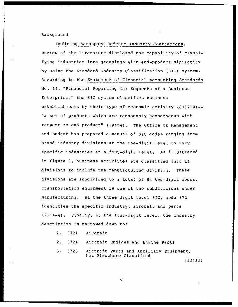
specific industries at a four-digit level. As illustrated

ir Figure 1, business activities are classified into 11

divisions to include the manufacturing division. These

divisions are subdivided to a total of 84 two-digit codes.

Transportation equipment is one of the subdivisions under

manufacturing. At the three-digit level SIC, code 372

identifies the specific industry, aircraft and parts

(22:A-4). Finally, at the four-digit level, the industry

description is narrowed down to:

1. 3721 Aircraft

2. 3724 Aircraft Engines and Engine Parts

3. 3728 Aircraft Parts and Auxiliary Equipment,Not Elsewhere Classified

(13:13)

5

Each of these narrow industry descriptions comprises only

one in over 1,000 classifications at the SIC four-digit

level.

333 77777 2223 3 7 2 2

33 7 23 3 7 22333 7 22222

Aircraft and Parts

Transportation Equipment

Manufacturing

Figure 1. SIC Code 372 Breakout (21:1-3)

Financial Ratios. "Financial ratios are an important

tool in analyzing the financial results of a company and in

managing a company" (12:19). This statement was a result of

a questionnaire sent out in the early 1980s to controllers

of the companies listed in Fortune's "Directory of the 500

Largest Industries, 1979." "To be useful, ratios must

express significant relationships" (17:758). Through the

years literally hundreds of these relationships have been

expressed. Based on their inclusion in recently published

literature and the availability of data, this research will

address multiple financial ratios in seven categories:

(1) Cash Position, (2) Liquidity, (3) Working Capital/Cash

Flow, (4) Capital Structure, (5) Debt Service Coverage,

(6) Profitability, and (7) Turnover (11:60). A description

6

and the significance of each of these categories follows.

The ratios proposed by this research are meant to be

illustrative not exhaustive. Specific ratios with formulas

are broken out by category in Table 1 (11:61-68).

1. Cash Position - The pool of funds (cash + marketablesecurities) that a firm can use to meet its cashobligations. The higher these ratios are, "the higher thecash resources available to the firm" (11:61).

2. Liquidity - Evaluates debt-paying ability of a companyby considering not only its ready pool of funds, but aswell, additional assets that can potentially be liquidatedquickly (7:352, 11:61).

3. Working Capital/Cash Flow - Identifies the cash-generating ability of firms. The higher each of the ratios,the larger the working capital/cash flow, that can begenerated (11:62, 64).

4. Capital Structure - Specifies "proportion of assetsfinanced by nonshareholder parties" (11:65). The higher theratio, the higher the proportion and the decreased means ofa firm "to finance assets which earn returns for the owners(2:486).

5. Debt Service Coverage - Indicates company's ability topay interest payments due to "nonequity suppliers ofcapital" from current operating income (11:66).

6. Profitability - Associates the amount of resources usedwith the amount of income earned (i.e., measures efficiency)(2:478). "The higher each of these ratios, the moreprofitable the firm" (11:67).

7. Turnover - Provides some measure of the liquidity of afirm's inventories. The larger the ratio the faster a firmcan expect to liquidate its inventory (7:484).

Problems and Limitations. While "ratios are among the

best known and most widely used tools of financial

analysis," one must stay aware of their limitations (1:34).

The validity of the ratio computations must be evaluated

7

a)-4

'-4

-44

w a) 0

+ -4 0O>

4.) 41J 41Ja) (U w to Wa)a r C q .. (a0 cUr)N

a) a) a)~ 41 .0C (1) CS E 2-4- 02a Oa) 0

.41 .J 4.) -4 4.3 x a0. 4-1 cd)

020W 0) 02-4 U 2 U a)a) a) a) 1).0 a a) (a 0 0>~ r4 >( 1.J -4 m20 4.1 En

C 4 -'c C: -4~ w (a En4 a)0rl - U3 to 3 ) 02.- 4.)

2-'4 wa a)- NW a,42 ~ ~ 0.

W0 W0 V) N - a) ~- ) 4J ) -44.J (A20a)( a)fn Q) a) 1-4 4 .,4 C 4-) (UO i0 0

E- -- 5 E-4 W of0&2 (am -0 4-) ~ C 0E-4

0cC 0 41 0 M2 (a .0 Q) a) Q) 0 0U) 02 a)Q Ac0 .0 S~ :: 2U 2z 22 0

4.1 ( W EnE-4 0 0 . 00 0 00 - w 0)',4- a)~ 63 )4 00( N-4

S+~ + + C 44 E- cl wC C 0.2 1 a) -4 I-4 P-4 -4 1-4

0 w .0 . .V .. 01 (13 .

C4 .q 0 02 02 02 W U 412 4 4130) 41 413 -4 U2

6-1 l (a (V (a z 0 m 0 0 (U (a a)Q) m 0wa E- v u zu ul uu z

E-4

-4-

(UUCu

4-4

00 (1

(D 41-, 494

m a)) Ma)

C)- 0o0- ( ) w :UU 4.1 U a E

-44

based on the validity and consistencies of the data being

computed (1:35). Specifically, any analysis must consider

not only the internal operating conditions, but also general

business conditions, industry position, management policies,

and as well accounting principles. In evaluating ratios,

the most predominant constraint involves the potential

inconsistencies due to alternative methods of inventory

valuation; e.g., First-in First-out (FIFO) versus Last-in

First-out (LIFO) (1:105).

On the other hand, "nonuniformity of accounting methods

across firms does not necessarily imply noncomparability of

financial statement-based ratios" (11:184). Although some

research on the LIFO/FIFO inventory alternatives have

stressed single instances of large dollar differences, other

studies of larger randomly chosen samples had quite

different results. Instead, their findings suggested

"little differences in the ranking of firms if either

inventory valuation method is consistently used" (5:225;

10:187). Furthermore, while there are adjustment techniques

available, there presently is "limited evidence on the

accuracy of these techniques" (10:192). Finally, there is

the option available of not making any adjustment. This

option is based on "the assumption that the change is

immaterial or that the change is an appropriate response by

management to (say) a shift in the underlying business

enviroment" (11:215).

9

Methods of Financial Analysis with Ratios. Extensive

empirical research concerning the financial state of a firm

has resulted in several methods of financial analysis with

ratio comparisons to include: (1) Beaver's Univariate

Model, (2) Altman's Z-Score Model, (3) The Zavgren Model,

(4) The Financial Capability (FINCAP) Analysis Method, and

(5) Robert Morris Associates Statement Studies. A brief

summary of each of these methods follows:

1. Beaver's Univariate Model. Published in 1966 in

the Journal of Accounting Research, the article, "Financial

Ratios as Predictors of Failure" by W. Beaver described a

discriminant analysis technique that used a univariate

approach. His concept of ratio analysis, a cash flow model,

viewed each firm as a "resevoir of liquid assets, which is

supplied by inflows and drained by outflows" (23:3).

Through individual analysis of 30 ratios, 6 were chosen as

the "best in classifying firms as failed or not failed:"

(1) Cash flow to total debt, (2) Net income to total assets,

(3) Working capital to total assets, (4) Total debt to total

assets, (5) Current ratio, and (6) The no-credit interval

(23:8). To choose these 6, Beaver performed a dichotomous

classification test on a sample of 79 failed and 79 non-

failed firms. This test first ranks each firm by the value

of a specific ratio. Then an "optimal" cutoff point for

predicting bankruptcy is determined by visually inspecting

the ranked ratios and choosing the value which "minimized

10

the total misclassification percentage" (11:542-543).

Despite limitations of statistical design, Beaver's study

obtained "a fairly high predictive ability with a simple

model" (23:9). Difficulties with his model include restric-

tion to the 30 original ratios based on their popularity in

literature. More important ratios may have been eliminated.

Additionally, due to techniques designed to alter ratio

values, "the predictive ability of popular ratios may be

unreliable" (23:9). More importantly, Beaver's univariate

approach is limited in that different ratios are used to

classify firms individually, and the potential exists for a

firm to receive conflicting classifications (23:10). Since

no single ratio has been able to capture the multidimensions

of a firm's financial status, several authors have published

research using multiple discriminate analysis. One of the

more popular models follows.

2. Altman's Z-Score Model. In 1968, E. Altman

published in The Journal of Finance his article titled

"Financial Ratios, Discriminant Analysis and the Prediction

of Corporate Bankruptcy." He researched the use of modern

statistical techniques with regards to ratio analysis.

Using a discriminate analysis technique, Altman attempted to

demonstrate that a multivariate approach could improve

bankruptcy prediction and be useful in practical applica-

tions (23:15).

11

Evaluating data from a sample of 33 bankrupt and 33

non-bankrupt firms, a discriminant function was selected

containing 5 of the original 22 variables Altman selected.

"Those selected did not include variables that would have

been considered the best predictors if evaluated on an

individual basis" (23:16). The function selected was:

Z = .021 * Xl + .041 * X2 + .033 * X3 + .006 * X4 + .999 * X5 (1)

where:

X1 = working capital/total assets,X2 = retained earnings/total assets,X3 = earnings before interest and taxes/total assets,X4 = market value equity/book value of total debt,X5 = sales/total assets, andZ = overall index.

Altman's model was significant as the first to evaluate

the ability of combining several ratios to assess a firm's

financial well-being. Still, the problem remained of

restriction of the original 22 ratios to a judgmental

selection. Table 2 illustrates that Altman achieved higher

accuracy than Beaver, especially for the first year prior to

bankruptcy (23:4). Given a longer time interval though,

Altman's predictive accuracy decreased drastically, while

Beaver continued to reasonably predict even five years prior

to failure.

12

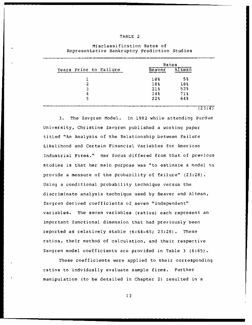
TABLE 2

Misclassification Rates of

Representative Bankruptcy Prediction Studies

Rates

Years Prior to Failure Beaver Altman

1 10% 5%2 18% 18%

3 21% 52%4 24% 71%

5 22% 64%

(23:4)

3. The Zavgren Model. In 1982 while attending Purdue

University, Christine Zavgren published a working paper

titled "An Analysis of the Relationship between Failure

Likelihood and Certain Financial Variables for American

Industrial Firms." Her focus differed from that of previous

studies is that her main purpose was "to estimate a model to

provide a measure of the probability of failure" (23:28).

Using a conditional probability technique versus the

discriminate analysis technique used by Beaver and Altman,

Zavgren derived coefficients of seven "independent"

variables. The seven variables (ratios) each represent an

important functional dimension that had previously been

reported as relatively stable (6:64-65; 23:28). These

ratios, their method of calculation, and their respective

Zavgren model coefficients are provided in Table 3 (6:65).

These coefficients were applied to their corresponding

ratios to indvidually evaluate sample firms. Further

manipulation (to be detailed in Chapter 2) resulted in a

13

TABLE 3

Zavgren Model Variables and Coefficients

Ratio Calculation Coefficient

Inventory Turnover Avg Inv/Sales .00108

Receivables Turnover Avg Rec/Avg Inv .01583

Cash Position (Cash + Marketable .10780

Securities)/TotalAssets

Short-Term Liquidity (Cash + Marketable -. 03074

Secur it ies) /CurrentLiabilities

Return on Investment Income/(LT Debt + -. 00486SH Equity)

Financial Leverage LT Debt/(LT Debt + .04350

SH Equity)

Capital Turnover Sales/(Total Assets - -. 00110

Current Liabilities)

(6:65)

measure of a firm's propensity to fail" (23:25). As in the

previously mentioned studies, the choice of ratios used was

"based on prior empirical evidence." Further analysis of an

expanded variable set was recommended (23:30).

4. The FINCAP Analysis Method. Published in 1979,

FINCAP Analysis describes a method used by AFSC contracting

personnel in the late 1970s through early 1980s to evaluate

the financial capability of major Air Force contractors

(18:1-1). An integral part of the FINCAP Analysis method

was the Contractor Financial Data and Analysis System

14

(FINANDAS) (18:2-10). FINANDAS was a timesharing computer

program which incorporated a data bank containing five years

of historical data on selected companies. Data were com-

piled from COMPUSTAT, DOD data, and prospective contractor-

supplied data (14:418). It had the capability to calculate

ratios and trends, and project future financial data.

Specifically, FINANDAS computed 22 individual ratios in 5

different classifications: (1) Performance, (2) Capitaliza-

tion, (3) Liquidity, (4) Coverage, and (5) Facilities

(18:11-6-10). Additionally, the FINANDAS system was

designed to automatically calculate and present Altman's Z-

score as previously described (18:11-10-11)

5. Robert Morris Associates (RMA) Statement Studies.

Annually, RMA publishes statement studies based on data

voluntarily submitted from its member banks. These studies

contain ratio "guidelines" categorized by SIC code. They

are presented as "guidelines" versus absolute industry norms

due to their nonrandom selection. There are three values

calculated for each ratio: the median and the upper and

lower quartiles (19:7). They are derived by listing the

values per company of each ratio in an order from the

strongest to the weakest. These arrays of ratio values are

then "divided into four groups of equal size" (19:7). The

median is the mid-point while the upper and lower quartile

points split the upper half and lower half (see Figure 2)

(19:7). RMA includes 16 different ratios under 5 principal

15

categories: liquidity, coverage, leverage, operating, and

specific expense items (12:8). Six of these ratios

(current, quick, COGS/Inventory, Sales/WC, Income/Interest

Expense, and Sales/Total Assets) will be compared with the

findings of this study in Chapter 3.

StrongRatios

25% ofRatios

Upper \ /Quartile - *

25% ofRatios

Median - *

25% ofRatios

Lower \Quartile - *

25% ofRatios

WeakRatios

Figure 2. Quartile Illustration(Printed with permission of RMA) (19:7)

Summary

This chapter identified the need for financial ratio

benchmarks for the aerospace industry as the specific effort

of this thesis. It introduced four research questions and

16

then, through a review of the literature, answered the first

two by (1) defining the aerospace industry using the SIC

system, and (2) specifying the fourteen ratio benchmarks to

be provided and the information given by each. The fourth

question was addressed in the section on problems and

limitations. The chapter concluded by summarizing several

examples of past research and actual use of financial

analysis with ratio comparisons.

Utilizing some of the statistical techniques derived

from reviewing the literature, the next chapter details the

methodology used to address the research question concerning

both how ratio benchmarks are calculated and how to test

their statistical significance.

17

II. Methodology

Overview

The previous chapter provided an introduction to the

research problem (i.e., the need for aerospace contractor

financial ratio benchmarks). It provided a review of the

relevant literature pertaining to definition of an industry,

and discussion of financial ratio categories aLad various

analysis methods.

The purpose of this chapter is to describe the research

techniques to be used to answer the third research question.

The objective is to determine statistically significant

financial ratio benchmarks for evaluation of aeronautical

defense contractors. The general methods will focus on

manipulation and extraction of financial ratio data from the

Standard and Poors' computerized data file, Compustat, and

statistical analysis of the significance of the derived

benchmarks.

Defining the Industry

As stated in Chapter 1, the Standard Industrial

Classification (SIC) of industries is consistent with the

definition for end-product of an industry. For this

research, the three-digit SIC code 372 will be used to

define the aerospace industry.

18

Calculating Benchmarks

Financial ratio benchmarks will be calculated using the

data file, Compustat. The capabilities of a computer based

data file allow one to store, access, sift and manipulate

data mathematically, and could accomplish almost instantly

what could very well require weeks of manual input (1:43).

Compustat, a service of Standard and Poors' Corporation,

available at the University of Dayton in Dayton, Ohio, will

be used to accomplish this research. The Statistical

Analysis System (SAS) program produced to accomplish this

effort is included in Appendix A.

A benchmark or average can be measured by several

statistics (11:105). Most commonly they are measured as the

mean or the median. The mean is calculated as the sum of

the values divided by the number of values. The median is

computed by first ranking the observations from highest to

lowest, and then choosing the ratio in the middle. For an

even number of observations, the median is calculated as the

mean of the middle pair (16:12). Although this research

will present the mean values, it will concentrate on the

median as the industry norm. Reasons for this decision stem

from the median statistic's ability "to eliminate the

influence which values in an 'unusual' statement would have

on an average" (19:7).

19

Defining the Population

The population of contractors included in the research

will be restricted by the availability of SIC code 372

companies included in the Compustat data file. Additionally,

the research will only include companies which have

contracted with the Aeronautical Systems Division (ASD) since

1980. Data extraction will include multiple ratios per

company per year for the past decade (1978-1987).

Statistical Analysis

Standard Deviation. Although a midpoint or "norm" of a

distribution may be something to aim for, a reasonable range

of dispersion is to be expected. The standard deviation

sLatistic is one of the most common for measuring this

characteristic of data distribution. The standard deviation

is typically used to compare the dispersion in populations

with similar mean values. But it can also be used to

"estimate the percentage of population members that lie

within a specified distance of the mean" (16:19). For many

large populations with normal distributions, the "rule of

thumb" is about 68% of the values lie within one standard

deviation of the mean, and approximately 95% lie within two

standard deviations (16:20). Additional research promotes

the expectation that less than 1/9 of a population will fall

outside three deviations from the mean (10:170). Chapter 3

will evaluate each of the 14 ratios in regards to their

compliance with these expectations.

20

High Quartile - Low Quartile Range. As discussed in

Chapter 1, a common determination of a reasonable range for

a ratio are the central "quartiles" or middle 50% of a

population, thus eliminating the "unusual" values (19:7).

Many, perhaps most, ratios are expected to have nonnormal

distributions greatly reducing the significance of the

standard deviation--a statistic which assumes a normal

distribution (11:102). Many ratios have the technical lower

limit of zero; others have a top limit of one or are just

naturally skewed. By examining the "fractiles or

percentiles of the distribution rather than focusing only on

the mean and standard deviation," a more accurate range of

ratio values should be reflected (11:104; 19:7). Chapter 3

will present the point values of the high and low quartiles.

Analysis will include determination of whether the inner

quartiles fall within a single standard deviation from the

medians.

Other Measures of Dispersion. Due to their current

growing popularity in the literature, two other measures of

dispersion will be presented and analyzed: (1) the

variability measure and (2) the studentized range.

Variability Measure. The objective of the

variability measure is to "expand beyond one fiscal year the

information contained in a single ratio measure" (11:72).

It is simply calculated as:

Maximum Value - Minimum Value (2)Mean Financial Value

21

Studentized Range (SR). The SR statistic "tends

to be 'large' for fat-tailed distributions" (11:107). It is

calculated as:

Maximum Value - Minimum Value (3)Standard Deviation

With observations exceeding 100, the published rule of thumb

for suspecting distributions to have fat tails is an SR

value greater than 6.5 (11:107).

Cross-Section Correlation. A cross-sectional analysis

is used to "examine the correlation between financial ratios

of firms at a point in time" (11:114). This correlation is

extremely important when combining financial ratios to

create a single measurement of a firm's financial health.

High correlation (multicollinearity) between variables of a

model results in model coefficients which may be very

sensitive to sample size changes. Due to the previously

mentioned "non-normal" distributions of many ratios, the

Spearman rank correlation (a statistic that does not assume

normality) was chosen to test the correlation of this

study's 14 ratios (11:114). Calculation of the Spearman

rank correlation coefficient first requires a ranking of

observation (company) values for each ratio from strongest

to weakest. Ratios rankings are paired one at a time,

differences of the two ratio rankings per company are

calculated and then squared. The Spearman rank correlation

coefficient is then calculated as:

22

1 - ((6 * sum of squared difference)/(N cubed - N)) (4)

where N is the number of observations (companies).

Time-Series Trends. Comparable ratio values of earlier

fiscal periods should be carefully studied to determine

trends. Any significant trend should be given consideration

with the effect of the trend incorporated into the benchmark

determination. Approaches to this analysis include

(1) visually examining the data and (2) using statistical

tools to detect significant systematic patterns in the data

(11:218). To enhance a visual examination, Appendix B will

include graphs illustrating the trend of the yearly medians

per ratio. Additionally, these medians will be statis-

tically evaluated using (1) the autocorrelation function

and (2) performing linear regression.

1. Calculating the Autocorrelation Coefficient.

This coefficient is estimated as (11:32):

Sum of ((Xt) - 7) ((X(t+j)) - K) (5)

var iance

where

7 designates the "mean" of the observations

Xt designates the observation being calculated; tranges in value from 1 to T-j

T designates the total number of observations

j designates the lag of time between specifiedobservations (for this research, j = 1)

23

Theoretically, for a population with truly random

changes, this coefficient would equal zero (11:232). In

actuality, one cannot expect estimated autocorrelation

coefficients to be exactly zero. Instead, as a "general

rule of thumb", a coefficient can be determined

"significantly different from zero if the sample estimate is

more than two standard errors from zero" (11:233). The

standard error (SE) equals:

SE = square root of (1/(T - j)) (6)

with T = 10 years, and j = 1:

SE = square root of 1/9 = 1/3. (7)

Thus, for this sample to be significant, a coefficient

value must either exceed +.666 or be less than -. 666.

2. Testing with Linear Regression. Due to its

ability to determine the existence of a relationship between

two or more quantitative variables, this study also will

include regression analysis to evaluate potential time-

series trends (15:23). Separately, each financial ratio

yearly median (the dependent variables) will be compared

with the independent variable "year." The study's

regression model will be:

Financial Ratio Yearly Median = a + b(year) + e (8)

where

a = the Y intercept

b = the slope fo the regression line

e = the random error term

24

Based on the 10 years/observations, a line of best fit

is computed using a SAS program. Additional statistics

including a "T" value are generated as requested. The "T"

value equals the slope of the line divided by the estimated

standard error of the slope. This statistical value tests

whether the slope of the fitted line is significantly

greater than or less than zero. A significant slope would

demonstrate an upward or downward trend in a financial ratio

median between 1978 and 1987. To test the "T" values

calculated by SAS, specific research bypothesis and decision

rule are as follows:

Null and Alternative Hypothesis: H0 : b = 0 (no trend)

Ha: b / 0 (trend)

Decision Rule: If the absolute value of "T" calculated

is greater than "T" critical, reject Ho; otherwise fail to

reject Ho (i.e., if b=0, then the ratio median of a

representative population sample is a "good" benchmark).

The "T" critical value is based on the significance

required and whether the test is one-tailed or two-tailed.

Since this research looks for both upward and downward

trends, the test is two-tailed. Due to its frequent use in

"classical hypothesis testing," a significance level of 0.05

will be used (13:265). Thus, based on these factors and

with eight degrees of freedom (ten observations less two

parameter estimates), the "T" critical value is 2.306

(15:518).

25

Zavgren's Model. As presented in Chapter 1, an index

representing the probability of a company's impending

failure can be derived by computing the Zavgren model with

company specific data. Each of the seven ratios are

calculated, and multiplied by both 100 and its respective

coefficient. The seven products are summed and the total is

added to -. 23883. This result, designated as 'y' is then

manipulated as follows (6:64):

Probability Index = l/(1 + e-Y) (9)

where

e is the base of natural logarithms.

The calculation of this model will be included as a

statistical analysis technique to examine the "financial

soundness" of the companies within the sample.

Summary

Chapter 2 presented the details of the main research

effort, and actual calculation and statistical analysis of

the financial ratio norms. It explained how the sample data

was determined; and furthermore, how the Compustat data file

was accessed, data extracted, and finally manipulated into

ratios (see SAS program in Appendix A). In conclusion, this

chapter laid the general framework for testing the

statistical significance of each benchmark.

Explicitly, the statistical definition of a benchmark

is the median ratio value of companies within a specific

26

industry. The inner quartile surrounding the median

presents an acceptable range of ratio values. To be

considered useful/significant, this range should come from

distributions which resemble normal in regards to a

tightness of values around the median. Additionally,

consideration of benchmark adjustment should be made for any

ratio distribution exhibiting a definite time-series trend.

Finally, although correlation between ratios doesn't affect

their significance when analyzed individually, these

relationships prove extremely important when combining

ratios to formulate a single index.

The next chapter contains the results of the data

extraction and manipulation into ratios. Overall medians,

low quartiles and high quartiles will be calculated and

displayed. Finally, results of statistical tests will be

presented and level of significance discussed.

27

III. Data Analysis and Findings

Introduction

The previous chapter described the methodology used to

compute financial ratio norms and techniques to test their

statistical significance. This chapter presents the

findings derived from the data and statistical analysis.

The first section describes the population sample members

that resulted from the restrictions detailed in Chapter 2.

The next section presents the derived "benchmarks" and their

respective inner quartile range points. The chapter

concludes with the results of several statistical analysis

techniques/tests outlined in Chapter 2.

Population Sample Description

A visual comparison of an ASD listing of contractors

utiliz-ed since 1980 and the listing of companies provided by

Compustat per the user manual, provided an original sample

set of 14 contractors. Due to circumstances surrounding two

of these companies (one had less than 10 years of data, and

one produced bad results due to denominator values of zero),

the list of companies was reduced to 12. These defense

aerospace industry contractors are as follows:

1. Allied Signal Corporation2. Boeing Company, Incorporated3. General Dynamic Corporation4. Grumman Corporation5. McDonnell Douglas Corporation6. Northrop Corporation7. Raven Industries Incorporated

28

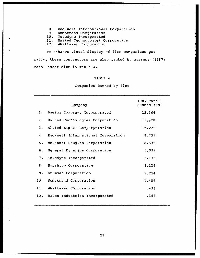
8. Rockwel' International Corporation9. Sunstrand Corporation

10. Teledyne Incorporated11. United Technologies Corporation12. Whittaker Corporation

To enhance visual display of firm comparison per

ratio, these contractors are also ranked by current (1987)

total asset size in Table 4.

TABLE 4

Companies Ranked by Size

1987 Total

Company Assets ($M)

1. Boeing Company, Incorporated 12.566

2. United Technologies Corporation 11.928

3. Allied Signal Corporporation 10.226

4. Rockwell International Corporation 8.739

5. McDonnel Douglas Corporation 8.536

6. General Dynamics Corporation 5.032

7. Teledyne Incorporated 3.135

8. Northrop Corporation 3.124

9. Grumman Corporation 2.254

10. Sunstrand Corporation 1.480

11. Whittaker Corporation .430

12. Raven Industries Incorporated .163

29

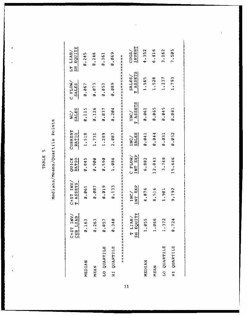
Calculated Benchmarks/Quartile Range

A benchmark for each of the 14 ratios was calculated

by first accessing through Compustat the required financial

statement values per company through 10 years (1978 - 1987).

A SAS program (Appendix A) performed the raw data extraction

and as well calculated the ratio values requested. To

facilitate graphing/worksheet analysis, the raw data were

re-input into a Quattro computer program. For each of the

14 different ratios, the 120 observations were ranked by

value, and their middle pairs were each totaled and divided

by two. These values (the medians), and the upper and lower

quartile points are exhibited in Table 5. The mean is also

presented for comparison purposes. Additionally, a compar-

ison with six corresponding ratios presented annually for

SIC Code 372 (aircraft and aircraft parts manufacturers to

include non-DOD as well as DOD contractors) by RMA is shown

in Table 6 (19:186).

Beyond an overall benchmark, separate medians were

calculated both by company and by year. These median values

are presented in Tables 7 and 8, and as well, their values

are graphically illustrated in Appendix B. Note the company

numbers assigned in Appendix B correspond to the listing of

companies by current total asset size (see Table 4).

Additional Statistical Results

Standard Deviation. The standard deviations of the

ratios measured by this research are presented in Table 9.

30

>4E-

r ~ ~ ~ N 1.4 k0 0. f 0 > ()r4 Ui)a 'f CJ2 U )) ,-4 11 0

E-4-

W MirJ %0 04I mi 7%U)c1 r- (*e) m C% 6j ' n U, Lo) 04 Ir-

O 0 r- ul OD

tm Is

IE-U2 Ln 40o Ir- ,T WI r -4 U) ItO -4

N2 -4 (1 It NC/3 IS m0 In

-- 4 1- c 0 IX E-4 ur 11 D I

-4 ~ -(Z Oct~~

(Z -4 r-4 14 C4 if -~f

0- Ol In m m 0 % II it it 04 c, co 40

4: ) '-E- 00 0' In IS 11 63 O 0 rE- c * * It Drs.E-4

Of Im t ,-4 11 Z o CN 04 V)

E It

C If

Z E-4 -ar a4I..4C W 0 kD -4 x -WXq' 4 4 0

EV Cn 11 U~ II 0C C .4

+ If 4-Z ~~~4

it

N Ii >4>I 11 E-4

(Z C- 1 It - In 40 CIS 1W-4 ~ 40 40 ) it D' If) t. 0 r- 04

014 m (1 if -40 a m m'

Co) Ix IS rs m Im 14 CD

00 r4 C4iW

P- -4 Ii4- -

E- E-' it E-. E-

z <: 4 ;i Z .4 t4

4- Z y 0 .'

Wi Wz 0 W Cz4 Q

31

c0

o .-4 11 >4 00 U ONb

U 0 r- lz CIt 4J

U C

fl In a

co 11 In 00.1U

r-4 .14 -1 (Y II it () - C -

:If III

4J4E

-- 11041 n - )-

.C C

44 r4 4 - if -4 -4

14 1 a0t U

'0~E- WCL IJ

Cz3~~4. 4C 41~ I U W .

-3 W 4U2 C~'l -4 -4l Of 0~*-C) I -Ua .CO

a) cQXvU

32

E'Il N m' m' N~ -4 wO m %D v -4 wcE- IN, z qw -4 10 m c m ~ w' m c IS"

" W N-4ccr- -4c cc MVMm rMV-4W-4%0CSI cC"O W4M a) LI) Waa aoi r -r- * *

0 r . . . . 0 . * . 0 * . . 11 C) r4 r-4

it cn W r- to- r 00 kD C4 -IS Nr cc 1011 Wz w) qm In M I LA) Ch .4 mOD cc w r.o

3:W 0 % Mr c ) Dc O 4)0 r4 Ia t ) . . . * . * . .o rz) iN O N r-n V~ qr %W rI %T r- 11 oc e4 r-4 -4 r-4 r- 4 -4 -(-4 r-4 4

la ~ ~ ~ 1 E-4~ 4 BU

10 1

:1 E-U) oNI -Nm 0wqWjt~~B I'l4MMILU rlC1I 4 . n I r 44wm mWQnr

W ~ r- -1- ML) 1 m 4a M1 f)I MMMC M V CD MM M

~ B -4

va E-'04 z -i 1 BU -c 0( I nL - -r -

W - a%- s-4 IV m %.D C4 00 00 w C B 11 -W~ M .-W ) rM V-4 M~ (N kD MV

0=0) 40r 4t 0 L A ( N4 C4

43 cn III - 4

> if U " en r--I cc 4 -4 -4 -4 -c

~4CI) * * * ***** * Ito>* 11* a. . .

+c Z -Z t a i I L A) a mr4it 0

U E-4 b4

N >4

C a-4 -W CN LA 0) M M M V 1V-C l LA (N (nV) LA.4 M Y)a -4 in LA (O"- M V. M N -4 00 r-4 A- M cc 00 M 11 IS N. C4 cc -I M~ cc 0 M L) r-4

E- . . . a a 0 a 0 . . * o it 6. W a . a a a * . aU) XBSC s s DM M m( s mi -l - 4C 4 Mr4I

+ D i E-'00 u 11

it11

>4 1- mZZ z ' -4B it0D Z4Z~onW>4>44W 11 Zuonw 4>4~lZ

ZOWW ' 0C =X -tZ OZ 3 00 = E E4

0oz6OUWOcmm 0EZ 3 uWOOMM

33

NE-4 NZ -Wt ONm%

- C'U2' WI In~ to mAo n m v W -4

w. . . . . .9 * * * I

It E

o4 I r- 'o. n or o %or- It 4 . . . . . . .*

4t . . . 9. 9 .* * E-cj2 m s mt mt s I

: * c . . . . * 1 * . . 0u .ts m2 m mt In It Z- ?s M M Cm CD IS *

fl E

x . . . . . II . 11 z>4 4 *4 * 94* * * * 4 1 -4 4 *

co .0 it~~Wit

it N

E- > = 9 . I r . . . . . . 9 a W .

OC m cIntm smmm it Z LnL)r . D 0mm-rk

-4 ~

>cn~ it E+ t 1 )OD%0 m mI 1 a

UE- ~ ~ ~ ~ ~ i xI-

11I 1- nm c

IN

61 C% 4 - % 4 - 4 4t 1 I N M M I 0C M 0 -E 1 4 4 . . . . . . 0 oEn x t t t t C Z M; t M; M* It 4F4m m+ m It .u u~it U

C41 0 ( 0 - " n 'WIn .0 " IZ CO N M 4 N(n wU) oIrr- r oDco c oooD o ooaD r-r- o ooco o oooo o o

34

E-4 E-4 qw tmo

M m w C4m .NZ -v un r- cm% r

6. IT -4

E- =E-

it EnCz w % 10-4 ML In t0 a

11~f C422 % ( -

cn m22 m t s

142 4 2V I-4U LnM r - 1 M mmC A r

W3 1-4 Iq m Nm- W2 m 1 4m Mr. 04 .0 0 4 . If 4 .22

z I V) %D w~- r-4C r-4 ff

4. It %Nn M22 IItl mM e S 1 O Smm t ;t

-4 "E-4 22OM MO O I -t r4C- Ln- X mC'4 SE-4 > 4 . I 1 4E4 . . .

Ze~~~~- 1-N r-W- r'44 22rnrC'd

00 Z2 E-C , a 012 0r4 1

M 0 0 22 r k l m 1 40 m 0I 0M -lM 00 r4Ul M 1 W I 0q0 rqc CV 0u OD

E-E- mE ?m12 Dm - - E' E'-U ~ - C 2 J r E224C l 14 .4 1

z 4 4CK -4 C 00 11 C -M(n mcI r>A' 4N m %D A 2 4 t C c J r - 0 N0

++ IE-' 1 E~ 1E- M + I-+ IE-

uU U E uuEIt UrE

3f

Additionally, this table reflects the results of analyzing

the normality of the distributions based on the count of

observations which fall outside the mean "+" or "-" either

one, two, or three standard deviations. As described in

Chapter 2, the "rule of thumb" for distributions of large

populations is about 68% of the observations lie within one

standard deviation while 95% lie within two. For this

somewhat large population of 120, this means only 38 of the

observations may fall outside one standard deviation, and

just 6 may fall outside two standard deviations. Three of

the ratios (WC/Sales, Lt Liab/SH Equity, and T Liab/SH

Equity) did not pass the one standard deviation test while

six of the ratios failed the two standard deviation test.

The additional published expectation that less than 1/9 of

the observations (in this case 13) fall outside of three

standard deviations is much more lenient and easily met.

Further analysis of the reasonableness of the inner

quartile range as compared with the standard deviation demon-

strated the high and low quartile points easily fell within

one standard deviation from the median for all ratios.

Variability Measure/Studentized Range. The two

additional measures of dispersion gave somewhat conflicting

results (Table 10). visual inspection of the variability

measure (Figure 3) illustrates a substantially higher

variability exists for two ratio categories, Cash Position

and Debt Service Coverage. The Liquidity Ratios and Capital

Structure Ratios demonstrated the lowest variability.

36

TABLE 10

Additional Measures of Dispersion

Variability Studentized

Ratios Measures Range

C+ST INV/CUR LIAB 7.797 6.269

C+ST INV/T ASSETS 5.954 5.388

QUICK RATIO 3.113 5.863

CURRENT RATIO 2.339 5.434

WC/SALES 3.813 4.178

C FLOW/SALES 2.754 5.633

LT LIAB/SH EQUITY 3.285 4.200

T LIAB/SH EQUITY 1.494 4.116

INC/INT EXP 8.139 5.974

C FLOW/INT EXP 6.709 5.477

INC/SALES 4.461 6.570

INC/T ASSETS 3.595 6.256

SALES/T ASSETS 1.262 4.865

COGS/INVENT 5.224 5.641

37

VARIABILITY MEASURE

RATIOS

C+ST INV/CUR LIAR

C+ST INV,/T ASSETS

QUICK RATIO

CURRENT RATIO

WC/ SALES

C FLOW/SALES

LT LIAB/SH EQUITY

T LIAB/SH EQUITY

INC/INT EXP

C FLOW/INT EXP

INC/SALES

INC/T ASSETS

SALES/T ASSETS

COGS/INVENT

0 2 4 6 8 10

VARIABLE VALUES

Figure 3. Graph of Variability Measure

38

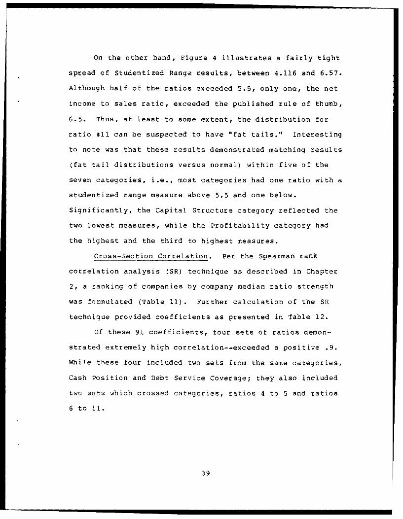
On the other hand, Figure 4 illustrates a fairly tight

spread of Studentized Range results, between 4.116 and 6.57.

Although half of the ratios exceeded 5.5, only one, the net

income to sales ratio, exceeded the published rule of thumb,

6.5. Thus, at least to some extent, the distribution for

ratio #11 can be suspected to have "fat tails." Interesting

to note was that these results demonstrated matching results

(fat tail distributions versus normal) within five of the

seven categories, i.e., most categories had one ratio with a

studentized range measure above 5.5 and one below.

Significantly, the Capital Structure category reflected the

two lowest measures, while the Profitability category had

the highest and the third to highest measures.

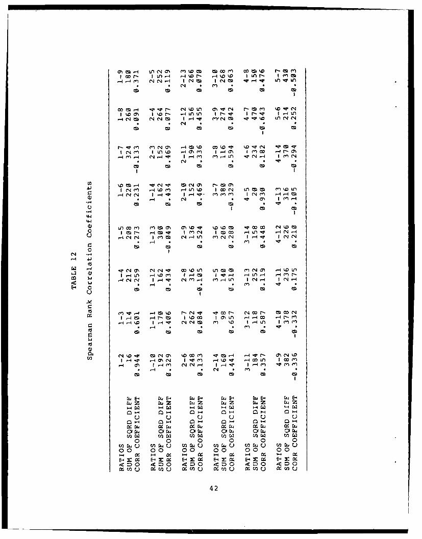
Cross-Section Correlation. Per the Spearman rank

correlation analysis (SR) technique as described in Chapter

2, a ranking of companies by company median ratio strength

was formulated (Table 11). Further calculation of the SR

technique provided coefficients as presented in Table 12.

Of these 91 coefficients, four sets of ratios demon-

strated extremely high correlation--exceeded a positive .9.

While these four included two sets from the same categories,

Cash Position and Debt Service Coverage; they also included

two sets which crossed categories, ratios 4 to 5 and ratios

6 to 11.

39

STUDENTIZED RANGE

RATIOS

C+ST INV/CUR LIAB

C+ST INV/T ASSETS

QUICK RATIO

CURRENT RATIO

We/SALES

C FLOW/SALES

LT LIAB/SH EQUITY

T LIAB/SH EQUITY

INC/INT EXP

C FLOW/INT EXP

INC/SALES

INC/T ASSETS

SALES/T ASSETS

COGS/INVENT

0 1 2 3 4 5 6 7

RANGE VALUES

Figure 4. Graph of Studentized Range

40

TABLE 11

Company Ranking by Ratio Strength

RATIOS: 1 2 3 4 5 6 7 8 9 10 11 12 13 14

COMPAN IES RANKING

Boeing 2 1 8 7 4 4 4 8 1 1 4 7 9 9

United T 10 10 10 6 6 9 6 6 10 11 9 8 6 10

Allied S 8 9 9 10 11 3 10 5 11 10 5 10 11 5

Rockwell 3 2 5 9 8 5 5 9 6 6 3 4 8 4

McD Doug 12 11 12 11 10 8 3 11 5 3 11 11 7 11

Gen Dyn 9 8 3 8 9 7 2 2 4 4 7 3 1 1

Teledyne 1 3 1 4 5 1 7 1 2 2 1 1 10 2

Northrop 7 6 11 12 12 11 1 10 3 5 8 5 2 3

Grumman 5 7 4 3 3 1212 7 12 12 12 12 3 7

Sunstrand 11 12 7 2 1 2 9 3 9 9 2 6 12 12

Whittaker 6 5 6 5 7 10 11 12 7 8 10 9 5 6

Raven Ind 4 4 2 1 2 6 8 4 8 7 6 2 4 8

41

ON *s 1-4 *l "~ *7 m *mmc n 0 0 0 r

r* . (I *q m* N M - -4q n1

t; * N m

1 %. 7 D r AV L - Ir 4 I

N * L)k - 4 N .n * -4o, OD 1-4r- 0

0 m r- WN" C1 I (7% r- m4U .4

(N (n4 1- D()I n% Drl U)m m M l

r4- .&4(nIJ

Cz~~~~~ -ts)N~ ((~l ~ u ~ 'N -t

44ia**

C1 -

C4 11** ~

CI2 4) 1 4 . - - 4m I -:r --4' 4 .- L r- r4 l)

- ' I-4 f 0'C I- I0 I-:r

(n IE Vz~E 4 4m% r-czi.0 00 C%4 o - m0

1 1-4 0 -4 r- M I-4z -400 m I) 4- 0 4r

%D qo m Nm k 0 0 0 A 04q - 0

-4 0 -4 M N4 CN r- -4 1 -4 M~ V4 ro

c~uU U2 ~(~U~C~U C'U CM

42

r- * 00 k~ *f m Or- eN m * l

OI I r- I-Dm -1r W r4M0

I - ( 4 I Iq1 -

-W N %D - *ot % .N k. VN m

M MImI-

CM~A,-U% r- ~- L 00 1-

C -) Ln(l rq- qN f) DR

-- 4-r-

Cat-r-

N I(C4 (N W N I ~CN (1 I.mNO wts)

4J 14q ') n% 1--4m 0 r- --4D U) .- 4UN .- Iq %

1 N *- *- V N 0) 1 * 1 N

a) ~ ~~ ~ ~ ~ -4- qW *-4 4% 1 s -4 - ,)mO

03-4O .4 O~ 4 N ~ (O

m I(N .- N No m ~ ~ u %D~ (M mk I< D 1."N

-4"0) - 0 -z . r- 4 0'AZ Lnz r- 1- 0 zw M r- 1 4 y)' I 0MI()C1 - -

w U) r- 00 m04- m9- -44 In 1-4 4

00 m -00-1Nu 4 00 -00 0094 (n C4 4 %0 C -C -4 Ln '-4 m I- v

CI 0C14 0 OD 0 .dq -4 a% m 4% O0wr N

43 -443 43

While four coefficients were very high, 75% of the 91

sets had an absolute value less than .5. Fifteen of the

remaining reflected a positive correlation between .5 and

.72, while four of the coefficients exhibited a negative

correlation which exceeded 0.5. Only one of these four

exceeded an absolute value of .7; a -.804 between ratios six

and thirteen. Once again, these two sets represented

comparisons of ratios of different categories. Of note,

only two other categories, Liquidity Position and

Profitability demonstrated any within category correlation,

and then only with a .657 and a .671, respectively.

Time-Series Trends. As presented in Chapter 2, three

time-series techniques were used to detect significant

systematic patterns in the data. First, a visual exami-

nation, as presented in the lower graph of each page in

Appendix B, illustrated little significant trend in all the

ratios except Ratio 5 (WC/Sales) which appeared to present a

somewhat upward trend.

Following the visual examination, two methods of

statistical evaluation were performed, autocorrelation

function analysis and regression analysis. Table 13

provides these statistical results. Testing of the

autocorrelation function found no coefficient values

exceeded the amount that would reflect significance, i.e.,

the two standard error calculation (.666). Only one ratio

44

TABLE 13

Time Series Analysis - Statistical Results

Autocorrelation Regression AnalysisRatios Coefficients "T" Values

C+ST INV/CUR LIAB 0.252 -2.125

C+ST INV/T ASSETS 0.399 -2.081

QUICK RATIO -0.189 -1.656

CURRENT RATIO 0.050 -1.401

WC/SALES 0.095 2.540

C FLOW/SALES 0.131 1.645

LT LIAB/SH EQUITY 0.522 -1.084

T LIAB/SH EQUITY 0.476 -0.883

INC/INT EXP 0.337 0.464

C FLOW/INT EXP 0.260 0.851

INC/SLAES 0.300 -1.230

INC/T ASSETS 0.343 -1.743

SALES/T ASSETS 0.345 -1.461

COGS/INVENT 0.259 -0.210

* Overall 12 companies for 10 years.

45

even appraoched this amount, Ratio 7. A repeated visual

examination of Ratio 7 (LT Liab/SH Equity) identified a

strong downward trend followed by an upward trend, but no

specific trend overall.

Finally, a regression analysis was performed on the

yearly medians. The "T" calculated values were compared to

the "T" table value of 2.306 (95% significance, two-tailed

test). Corresponding with the visual examination, Ratio 5

was the only ratio determined significant at above the 95%

level.

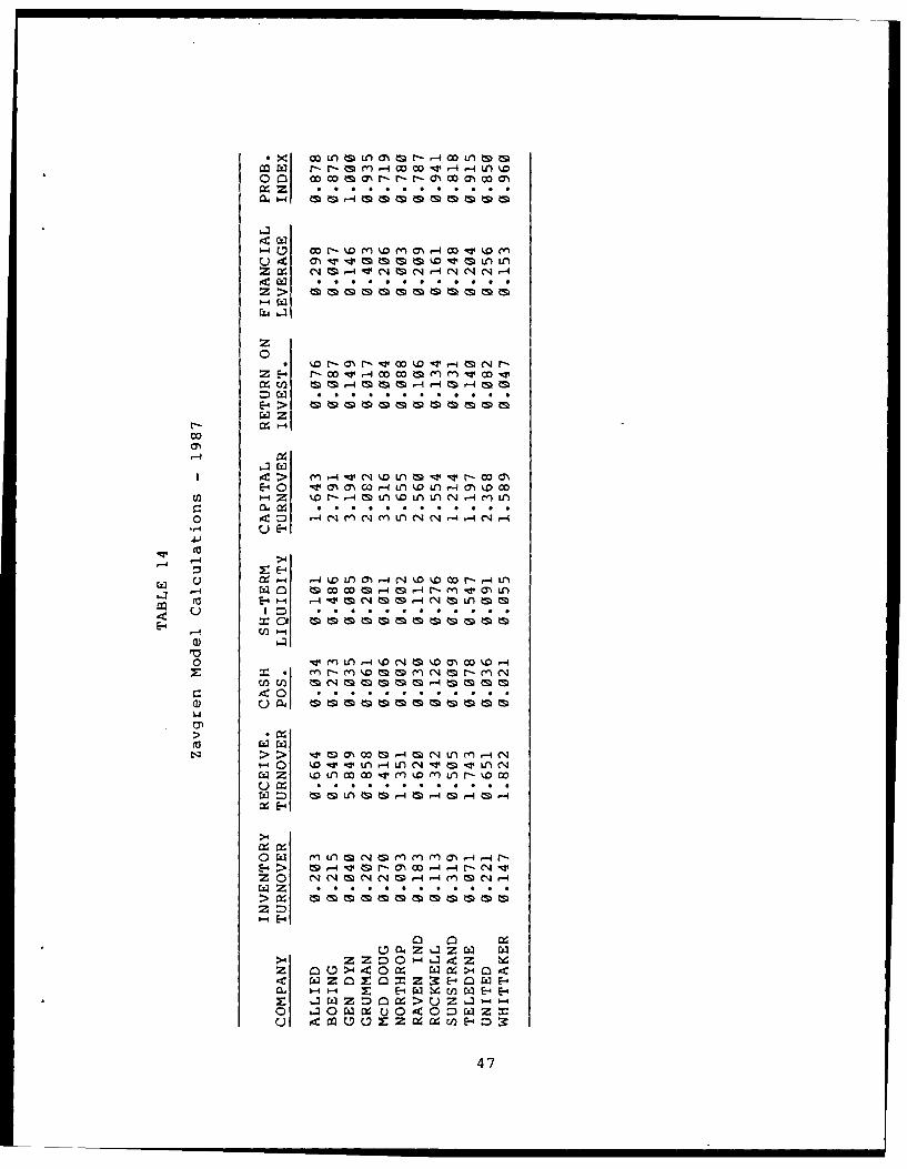
Zavgren's Model. As illustrated in Table 14, testing

of the Zavgren Model, on the 12 companies used in this

research, resulted in unreasonably high probability of

failure indices. An in-depth review of the model

formulation, to determine potential errors in this research,

revealed the model was applied correctly. Additional

literature from Zavgren disclosed an application of the

model (24:40-42). This application (the testing of a

securities company's ratios values for the five years prior

to bankruptcy) reflected values which at their best, worst,

and average were all inconsistent with the ratio values

derived by this thesis (24:41). Furthermore, the ranking of

the unreasonably high indices was compared by visual

inspection of each company's strength per individual ratio

(Appendix B and Table 11), and the Zavgren model ranking did

not correspond. These conflicting results demonstrate a

46

W0 LnM0m0r 4ML

r-4 r-m m - ;rrI- n

z

0

r-' 00 04-4 w m M v .

o2 M'- E->

E-4 04 n4( >G 44 k )- oc

0 4C- C t-4 COO --4N4 - C4 -

-4E-

4-)

>4

Z0 -4k U N D C - -4 )

r-4Z 0'4 ~

0 w n 4 DC4 D%0a CzZ E ~ - 00CD-4

0 nr V 10U0 MCDM 4 D - 1)Z

447

potential need for a model formulation based specifically on

defense contractors. An industry specific model could

better account for the unique conditions affecting these

companies.

Summary

This chapter contained the results of the financial

ratio calculations and statistical analyses. The derived

medians (benchmarks) and inner quartile range points were

presented in Table 5. Some of the ratios fell barely short

of meeting all the general "rules of thumb" as regards to

standard deviation(s) from the mean, yet all high and low

quartile points did fall within one standard deviation from

their respective medians. Additional dispersion analysis

techniques provided no consensus as far as identifying

potential distribution problems. Regarding correlation

between the ratios, Table 12 illustrated how 75% of the 91

ratio pairs had correlation of less than 0.5. The consensus

of the time-series trend analysis found only one ratio,

WC/Sales, reflected a significant trend suggesting a need

for benchmark adjustment. Finally, Table 14 presented the

results of the Zavgren Model as calculated on the sample

contractors.

The conclusions and recommendations relative to these

research findings are presented in the following chapter.

48

IV. Conclusion

Introduction

The previous chapters provided an introduction to the

research, a background review of the literature, a detailed

description of the proposed methodology, and the results of

the data computation and analyses. The specific objective of

this research was to provide ratio "benchmarks" representa-

tive to a specific industry definition. Based on this objec-

tive, this thesis presented the following research questions:

(1) How should the aerospace defense industry bespecifically defined?

(2) Which financial ratio benchmarks should be provided?What information does a specific ratio provide?

(3) How are specific ratio benchmarks calculated andtested for statistical significance?

(4) What problems result from financial ratio analysis?

This chapter will address these four questions and

discuss the results of this research as it pertains to each.

A final section of this chapter will provide recommendations

for future research.

Discussion of Results

Research Question 1. A background review of the litera-

ture as presented in Chapter 1 disclosed the capability of

defining aircraft and aircraft parts manufacturers by using

SIC code 372 of the Standard Industry Classification System.

To represent only defense contractors, this research

49

restricted its sample to include only companies which have

contracted with ASD since 1980. Using the Compustat data

bank and wanting only those with complete data from 1978-

1987, these restrictions allowed for a population sample of

12 defense contractors. These 12 representatives were

displayed on pages 28 and 29.

Research Question 2. A literature review revealed an

extensive list of ratios expressing numerous "significant"

relationships. The literatu.e disclosed that the choice of

ratios included in prior studies was largely judgmental and

usually based on their popularity in the literature. Due to

the need to confine the data to a reasonable/workable size,

this research addressed 14 ratios published in a 1988 book

by George Foster, Financial Statement Analysis. Although he

claims these ratios to be illustrative and not exhaustive,

as a published expert in the field of ratio analysis, this

researcher felt justified in selecting ratios from within

his seven main categories. These categories are: (1) Cash

Position, (2) Liquidity, (3) Working Capital/Cash Flow,

(4) Capital Structure, (5) Debt Service Coverage,

(6) Profitability, and (7) Turnover. Description of these

categories was displayed on page 7 with actual ratio

formulas on page 8.

Research Question 3. The focus of this study, the

calculation of the ratio benchmarks was determined in

Chapter 3. The methodology in the previous chapter has

50

defined the basic benchmark measurement as the median of the

sample observations. Additionally, Chapter 2 discussed the

need to reflect a reasonable range. The central quartile

was selected as this appropriate measurement. With these

measurements selected, the primary results of this thesis

were presented in Table 5 on page 31. One of the ratios,

WC/Sales, displayed a trend which signified a potential need

for adjustment to the values in Table 5. Examination of the

raw sample data revealed that while sales increased through

the years, WC grew by a larger percentage. Given that a

user assumes this trend to continue, the benchmark and

"reasonable range" points should be icreased by the

difference between the sample median and a forecasted value

based on a linear regressions line of best fit. The

remaining 13 ratios reflected no significant time series

trends. With no consensus on any abnormally high distri-

bution dispersion, the researcher believes these 13 ratio

norms reflect basic guidelines for comparison within the DOD

aerospace industry (assuming the sample is representative of

the industry).

A comparison with RMA's six comparable ratio medians,

and high and low quartile points (Table 6, page 32) demon-

strated that while the values were in the same "ball park,"

for the most part the broader industry definition by RMA

resulted in a broader inner quartile. This finding suggests

that a more specific industry definition can produce a more

representative norm.

51

Research Question 4. As stated in Chapter 1, the

problems associated with ratio analysis depend on the

validity and consistencies of the data being computed.

While the most predominate constraint involves the use of

alternative methods of inventory valuation, prior studies of

random sample companies found that these inconsistent

valuation methods resulted in minimal differences in company

ranking. Based on these studies and the lack of evidence on

available adjustment techniques, this researcher chose the

option available of not making any adjustment.

Still, it must be emphasized while ratio analysis is

helpful in appraising the present performance of a company

and in forecasting its future, it is not a substitute for

sound judgment nor does it provide a specific guide to

action. While the literature supports that a user is

clearly "better off with a ball-park estimate than with no

estimate at all," the usefulness of the ratio analysis is

dependent on the ability of the user to interpret its

meaning as it relates to other ratio values and as well any

peculiar conditions affecting the particular company or

industry as a whole (4:96).

Recommendations for Future Research

As previously noted, the ratios used in this study, while

popular in recent literature, are illustrative and not exhaus-

tive. Thus, beyond the beneficial value derived from the guide-

lines calculated, perhaps the more significant contribution of

52

this research is its support for further research. This section

will recommend a few of the many areas for future study.

First, a SAS program which took extensive time and

expertise to develop is now available (Appendix A). Small

adjustments could result in Compustat data access to allow

calculation of other ratios. Additionally, these ratios

and/or others could be calculated for other specific defense

industries, i.e., missile or artillery manufacturers.

Additionally, the researcher believes further study

should be devoted to formulating models corresponding in

nature to the Zavgren Model and Altman's Z-score Model. This

research's testing of ratio correlation (relationships) has

already laid some groundwork toward developing a model

specific to the aerospace defense industry. Based on these

relationships, relationships already determined by Zavgren's

and Altman's research, etc.; variables could be tested, with

coefficients and intercept calculated from industry-specific

data.

The final recommendation for further research concerns

the need to update the Defense Logistics Agency's Financial

Analysis Training Guide for Preaward and Postaward Financial

Analysis, dated September 1978. Additionally, a comparable

guide could/should be published to give program managers and

their cost analysts guidance with respect to the postaward

aspects of financial analysis. Along this line, the FINCAP

Analysis pamphlet and its related computer program/data

53

bank, FINANDAS, could be reevaluated concerning the

potential for their future use. Although canceled in the

early 1980s due to exhorbitant computer storage cost, a

future study of the use of FINANDAS could demonstrate that

its benefits now outweigh the current lower computer costs.

54

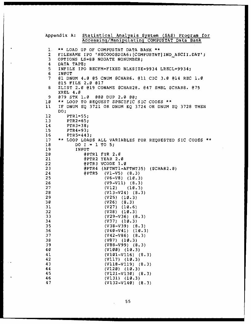
Appendix A: Statistical Analysis System (SAS) Program forAccessing/Manipulating COMPUSTAT Data Bank

1. ** LOAD UP OF COMPUSTAT DATA BANK **

2 FILENAME IPO 'HSCOOO$DUA6:[COMPUSTAT]INDASCII.DAT';3 OPTIONS LS=80 NODATE NONUMBER;4 DATA TAPE;5 INFILE IPO RECFM=FIXED BLKSIZE=9934 LRECL=9934;6 INPUT7 @1 DNUM 4.0 @5 CNUM $CHAR6. @11 CIC 3.0 @14 REC 1.0

@15 FILE 2.0 @178 ZLIST 2.0 @19 CONAME $CHAR28. @47 SMBL $CHAR8. @75

XREL 4.09 @79 STK 1.0 @80 DUP 2.0 @@;

10 ** LOOP TO REQUEST SPECIFIC SIC CODES **11 IF DNUM EQ 3721 OR DNUM EQ 3724 OR DNUM EQ 3728 THEN

DO;12 PTR1=55;13 PTR2=65;14 PTR3=38;15 PTR4=93;16 PTR5=443;17 ** LOOP LOADS ALL VARIABLES FOR REQUESTED SIC CODES **18 DO I- 1 TO 5;19 INPUT20 @PTRl FYR 2.021 @PTR2 YEAR 2.022 @PTR3 VCODE 1.023 @PTR4 (AFTNT1-AFTNT35) ($CHAR2.0)24 @PTR5 (VI-V5) (8.3)25 (V6-V8) (10.3)26 (V9-VlI) (8.3)27 (V12) (10.3)28 (V13-V24) (8.3)29 (V25) (10.3)30 (V26) (8.3)31 (V27) (10.6)32 (V28) (10.3)33 (V29-V36) (8.3)

34 (V37) (10.3)35 (V38-V39) (8.3)36 (V40-V41) (10.3)37 (V42-V86) (8.3)38 (V87) (10.3)39 (V88-V99) (8.3)40 (V100) (10.3)41 (VlO1-V116) (8.3)42 (V117) (10.3)43 (V118-VII9) (8.3)44 (V120) (10.3)45 (V121-VI30) (8.3)46 (V131) (10.3)47 (V132-V140) (8.3)

55

48 (V141) (10.3)49 (V142-V146) (8.3)50 (V147) (10.3)51 (V148-V162) (8.3)52 (V163) (10.3)

53 (V164-V174) (8.3)54 (V175) (10.3) @@;55 ** VARIABLE NAMES USED DISPLAYED AT END **

56 PTR1 + 2;57 PTR2 + 2;58 PTR3 + 1;59 PTR4 + 70;60 PTR5 + 1438;61 OUTPUT;6263 END;64 END;65 ELSE DO; INPUT; DELETE; END;66 INPUT;67 ** DELETION OF UNWANTED COMPANIES BY COMPANY SYMBOL **68 DATA NEW; SET TAPE;69 IF SMBL EQ 'PAR' OR SMBL EQ 'HEI' OR SMBL EQ 'UNC'70 OR SMBL EQ 'DCO' OR SMBL EQ 'MOG.A' OR SMBL EQ 'OEA'71 OR SMBL EQ 'PH' OR SMBL EQ 'RHR'72 OR SMBL EQ 'SER' OR SMBL EQ 'PSX'73 OR YEAR LE 77 OR YEAR EQ 88 THEN DELETE;74 ** RATIO CALCULATIONS **

75 RATIO1=Vl/V5;76 RATIO2=Vl/V6;77 RATIO3=(V1+V2)/V5;78 RATIO4=V4/V5;79 RATIO5=V121/V12;80 RATIO6=(Vl8+V125)/V12;81 RATIO7=V9/(V6-(V5+V9)) ;82 RATIO8 (V5+V9) / (V6- (V5+V9));83 RATIO9=VI8/V15;84 RATIO10=(V18+VI25)/VI5;85 RATIO11=Vl8/V12;86 RATIO12=V18/V6;87 RATIO13=V12/V6;88 RATIO14=V41/V3;89 ** PRINT VARIABLES BY COMPANY **

90 PROC SORT DATA=NEW; BY SMBL;91 PROC PRINT DATA=NEW NOOBS; BY SMBL;92 VAR YEAR Vi V2 V3 V4 V5 V6 V9 V12 VI5 V18 V41 V121 V125;93 ** CALCULATE RATIO STATISTICS PER EACH OF 14 RATIOS **94 PROC UNIVARIATE NOPRINT DATA=NEW;VAR RATIO1;95 OUTPUT OUT=RAT1 N=N MEAN=MEAN STD=STD MEDIAN=MEDIAN

MIN=MIN MAX=MAX;9697 PROC UNIVARIATE NOPRINT DATA=NEW;VAR RATIO2;

56

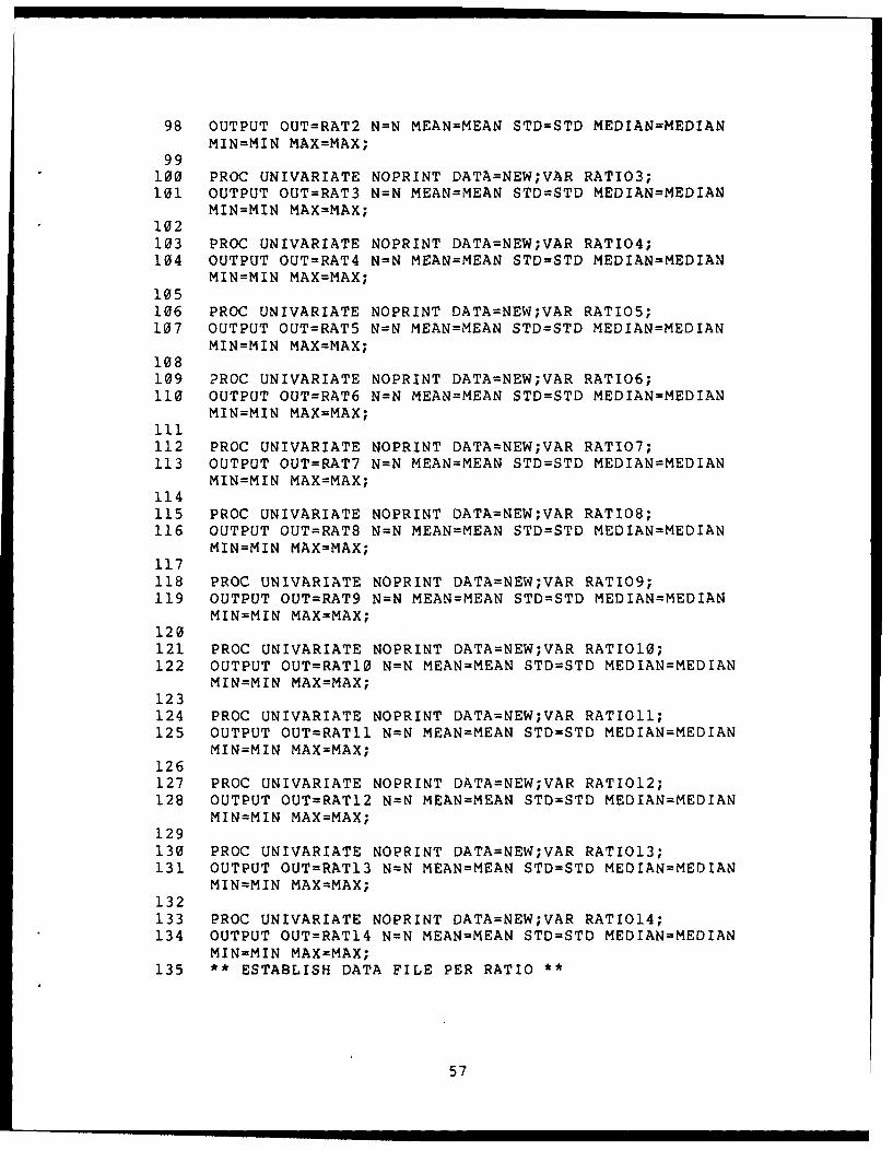
98 OUTPUT OUT=RAT2 N=N MEAN=MEAN STD=STD MEDIAN=MEDIANMIN=MIN MAX=MAX;

99100 PROC UNIVARIATE NOPRINT DATA=NEW;VAR RATIO3;101 OUTPUT OUT=RAT3 N=N MEAN=MEAN STD=STD MEDIAN=MEDIAN

MIN=MIN MAX=MAX;102103 PROC UNIVARIATE NOPRINT DATA=NEW;VAR RATIO4;104 OUTPUT OUT=RAT4 N=N MEAN=MEAN STD=STD MEDIAN=MEDIAN

MIN=MIN MAX=MAX;105106 PROC UNIVARIATE NOPRINT DATA=NEW;VAR RATIOS;107 OUTPUT OUT=RAT5 N=N MEAN=MEAN STD=STD MEDIAN=MEDIAN

MIN=MIN MAX=MAX;108109 PROC UNIVARIATE NOPRINT DATA=NEW;VAR RATIO6;110 OUTPUT OUT=RAT6 N=N MEAN=MEAN STD=STD MEDIAN=MEDIAN

MIN=MIN MAX=MAX;ill112 PROC UNIVARIATE NOPRINT DATA=NEW;VAR RATIO7;113 OUTPUT OUT=RAT7 N=N MEAN=MEAN STD=STD MEDIAN=MEDIAN

MIN=MIN MAX=MAX;114115 PROC UNIVARIATE NOPRINT DATA=NEW;VAR RATIO8;116 OUTPUT OUT=RAT8 N=N MEAN=MEAN STD=STD MEDIAN=MEDIAN

MIN=MIN MAX=MAX;117118 PROC UNI~hRIATE NOPRINT DATA=NEW;VAR RATIO9;119 OUTPUT OUT=RAT9 N=N MEAN=MEAN STD=STD MEDIAN=MEDIAN

MIN=MIN MAX=MAX;120121 PROC UNIVARIATE NOPRINT DATA=NEW;VAR RATIOlO;122 OUTPUT OUT=RAT10 N=N MEAN=MEAN STD=STD MEDIAN=MEDIAN

MIN=MIN MAX=MAX;123124 PROC UNIVARIATE NOPRINT DATA=NEW;VAR RATIOll;125 OUTPUT OUT=RAT11 N=N MEAN=MEAN STD=STD MEDIAN=MEDIAN

MIN=MIN MAX=MAX;126127 PROC UNIVARIATE NOPRINT DATA=NEW;VAR RATIO12;128 OUTPUT OUT=RAT12 N=N MEAN=MEAN STD=STD MEDIAN=MEDIAN

MIN=MIN MAX=MAX;129130 PROC UNIVARIATE NOPRINT DATA=NEW;VAR RATIO13;131 OUTPUT OUT=RAT13 N=N MEAN=MEAN STD=STD MEDIAN=MEDIAN

MIN=MIN MAX=MAX;132133 PROC UNIVARIATE NOPRINT OATA=NEW;VAR RATIO14;134 OUTPUT OUT=RAT14 N=N MEAN=MEAN STD=STD MEDIAN=MEDIAN

MIN=MIN MAX=MAX;135 ESTABLISH DATA FILE PER RATIO *

57

136 DATA ONE;137 SET RATI;138 RATIO='RATIO1';139140 DATA TWO;141 SET RAT2;142 RATIO='RATIO2*;143144 DATA THREE;145 SET RAT3;146 RATIO='RATIO31;147148 DATA FOUR;149 SET RAT4;150 RATIO='RATIO41;151152 DATA FIVE;153 SET RATS;154 RATIO='RATIO5';155156 DATA SIX;157 SET RAT6;158 RATIO='RATIO61;159160 DATA SEVEN;161 SET RAT7;162 RATIO='RATIO71;163164 DATA EIGHT;165 SET RAT8;166 RATIO='RATIO81;167168 DATA NINE;169 SET RAT9;170 RATIO='RATlO9v;171172 DATA TEN;173 SET RAT10;174 RATIO='RATIO10';175176 DATA ELEVEN;177 SET RAT11;178 RATIO='RATIO11';179180 DATA TWELVE;181 SET RAT12;182 RATIO=IRATIO12';183184 DATA THIRTEEN;

185 SET RAT13;186 RATIO='RATIO13';187

58

188 DATA FOURTEEN;189 SET RAT14;190 RATIO='RATIO14';191192 DATA TOTRAT;193 SET ONE TWO THREE FOUR FIVE SIX SEVEN EIGHT NINE TEN194 ELEVEN TWELVE THIRTEEN FOURTEEN;195 ** PRINT STATISTICS PER RATIO **

196 PROC PRINT; VAR RATIO N MEAN MEDIAN STD MIN MAX;197 ** PRINT RATIOS BY RATIO # SORTED BY COMPANY **

198 PROC SORT DATA=NEW; BY SMBL;199 PROC PRINT DATA=NEW NOOBS; BY SMBL; VAR YEAR RATIOl;200 PROC PRINT DATA=NEW NOOBS; BY SMBL; VAR YEAR RATIO2;201 PROC PRINT DATA=NEW NOOBS; BY SMBL; VAR YEAR RATIO3;202 PROC PRINT DATA=NEW NOOBS; BY SMBL; VAR YEAR RATIO4;203 PROC PRINT DATA=NEW NOOBS; BY SMBL; VAR YEAR RATIO5;204 PROC PRINT DATA=NEW NOOBS; BY SMBL; VAR YEAR RATIO6;205 PROC PRINT DATA=NEW NOOBS; BY SMBL; VAR YEAR RATIO7;206 PROC PRINT DATA=NEW NOOBS; BY SMBL; VAR YEAR RATIOS;207 PROC PRINT DATA=NEW NOOBS; BY SMBL; VAR YEAR RATIO9;208 PROC PRINT DATA=NEW NOOBS; BY SMBL; VAR YEAR RATIO10;209 PROC PRINT DATA=NEW NOOBS; BY SMBL; VAR YEAR RATIO11;210 PROC PRINT DATA=NEW NOOBS; BY SMBL; VAR YEAR RATIO12;211 PROC PRINT DATA=NEW NOOBS; BY SMBL; VAR YEAR RATIO13;212 PROC PRINT DATA=NEW NOOBS; BY SMBL; VAR YEAR RATIO14;213 RUN;

COMPUSTAT VARIABLE DEFINITIONS (20: Section 4 21-23, 27)

VI: Cash and Short-Term InvestmentsV2: ReceivablesV3: InventoriesV4: Current AssetsV5: Current LiabilitiesV6: Total AssetsV9: Long-Term DebtV12: Net SalesV15: Interest ExpenseV18: Income Before Extraordinary ItemsV41: Cost of Goods SoldV121: Working CapitalV125: Depreciation and Amortization

59

Appendix B: Graphical Display of Median Value Comparison

By Company/By Year Per Ratio

'87 TOTAL ASSETS ($B)

1. BOEING 12.566

2. UNITED TECHNOLOGIES 11.928

3. ALLIED SIGNAL 10.226

4. ROCKWELL 8.739

5. McDONNELL DOUGLAS 8.536

6. GENERAL DYNAMICS 5.032

7. TELEDYNE 3.135

8. NORTHROP 3.124

9. GRUMMAN 2.254

10. SUNSTRAND 1.48

11. WHITTAKER .43

12. RAVEN .02

*Companies listed by size (see Table 4)

60

(CASH & SHORT TERM INVESTMENTS)/

(CURRENT U1ABILITIES)

-~BENCHMARK 0. 163

0.7-

0 .8 -.........RA 0.5 -. ..TI0 0.4-

V 0.3-AL0.

0.1 -....

0-1 2 3 4 5 8 6 9 10 11 1'2

COMPANY

0.25-

R .

AT 01

0

A 0.1LuE

0.05-

0 7 ,8 7 19 810 8'1 82 8'3 84 85 881 8 7

YEAR

61

(CASH & SHORT TERM INVESTMENTS)/(TOTAL ASSETS)

BENCHMARK 0.061

0.3 - _ _ _ _ _ _ _ _ _ _ _ _ _ _ _ _ _ _ _ _ _ _ _ _ _ _ _

0.25-RAT 0.2I

A

E 0 .0 5. ...... . ...... .... ..... .. .-. .

0.08-

0.07

0.06

AT 00I0

0.04-vAL 0.03-uE 0.02

0.01-

0 7 ,8 7 9 8 10 8 11 8 12 8 13 84 85 881 8 17

YEAR

62

QUICK RATIO

-~BENCHMARK 0.845

1.4

R 1.2-AT 1 ....

00.8-

VA 0.6-L

E0.4-

0-1 2O 3' 4 0 1 2

COMPANY

1

RAT0.I0

VA 0.4LUE

0.2-

078 79 80 81 82 83 84 85 88 87

YEAR

63

CURRENT RATIO

-~BENCHMARK 1.518

3-

2 .5 --. .. ..... .

RAT 2-

01.5-

AL I - ..... .........

E0.5 -. .. .. .

0-1Is3 4 7 a 9 10 11 12

COMPANY

1.4 - ...

RA12TI

0

V 0.8ALu 0.8E

0.4

0.2

078 79 80 81 82 53 84 85 86 87

YEAR

64

(WORKING CAPITAL)/(SALES)

-~BENCHMARK 0.115

0.35 -_ _ _ _ _ _ _ _ _ _ _ _ _ _ _ _ _ _ _ _ _ _ _ _ _ _ _ _

0.3-

R 0.25 -.. ..AT 0.2-I0

0.15-VA 0.1 - ..L

U 0.05 -...... ....

0

.-0.05

COMPANY

0.18-.

0.1-6

RA 0.12-T

0 0.1-

V 0.08-ALU 0.06

0.04

0.02

78 7 9 80 8'1 82 8S3 84 85 86 87

YEAR

65

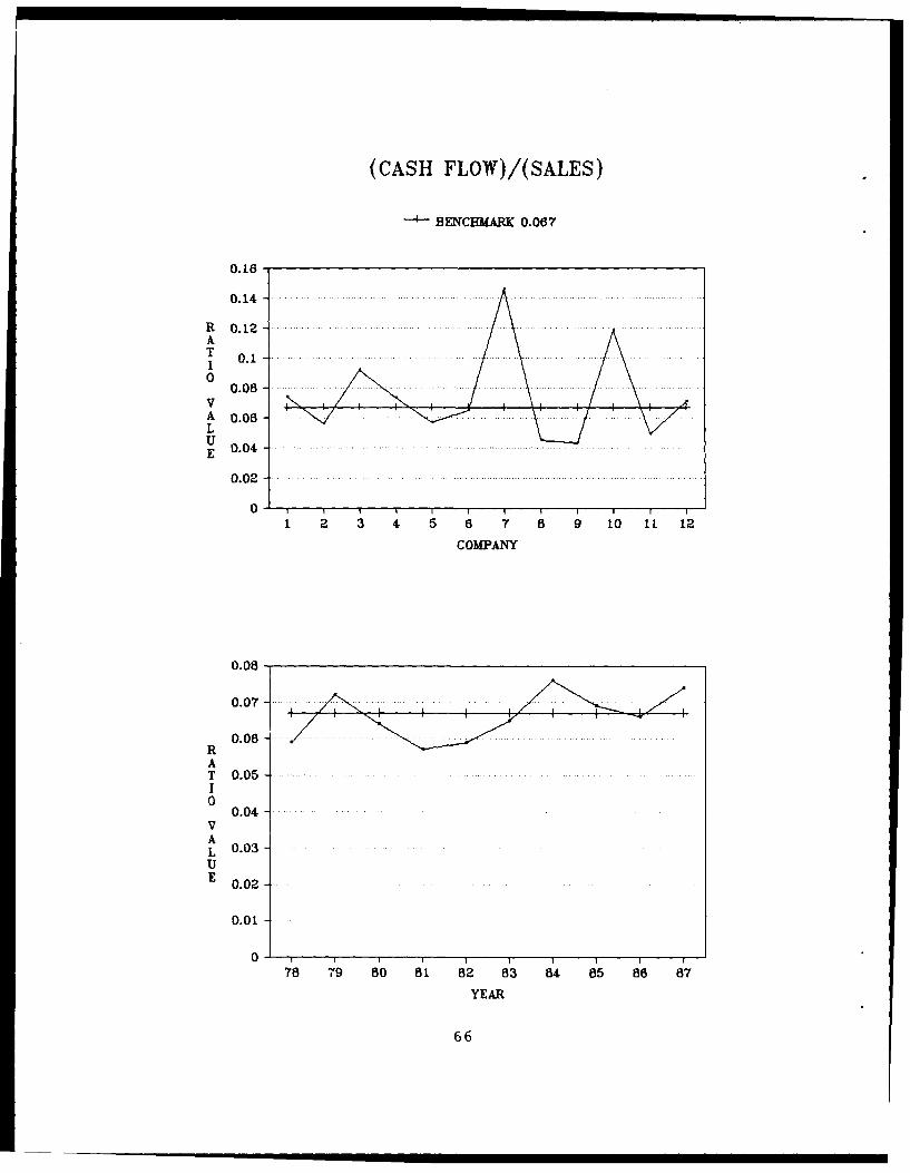
(CASH FLOW)/(SALES)

- BENCHMARK 0.067

0.16-

0.14-

R 0.12-AT 0.1I0

A 0.06 -....... .. 4

LU 0.04-E

0 .02 -. .. .. .. .... ....

0-

COMPANY

0:07-

0.06-RAT 0.05-I0

0.04-VAL 0.03-uE 0.02-

0.01

078 79 80 81 82 83 84 85 86 87

YEAR

66

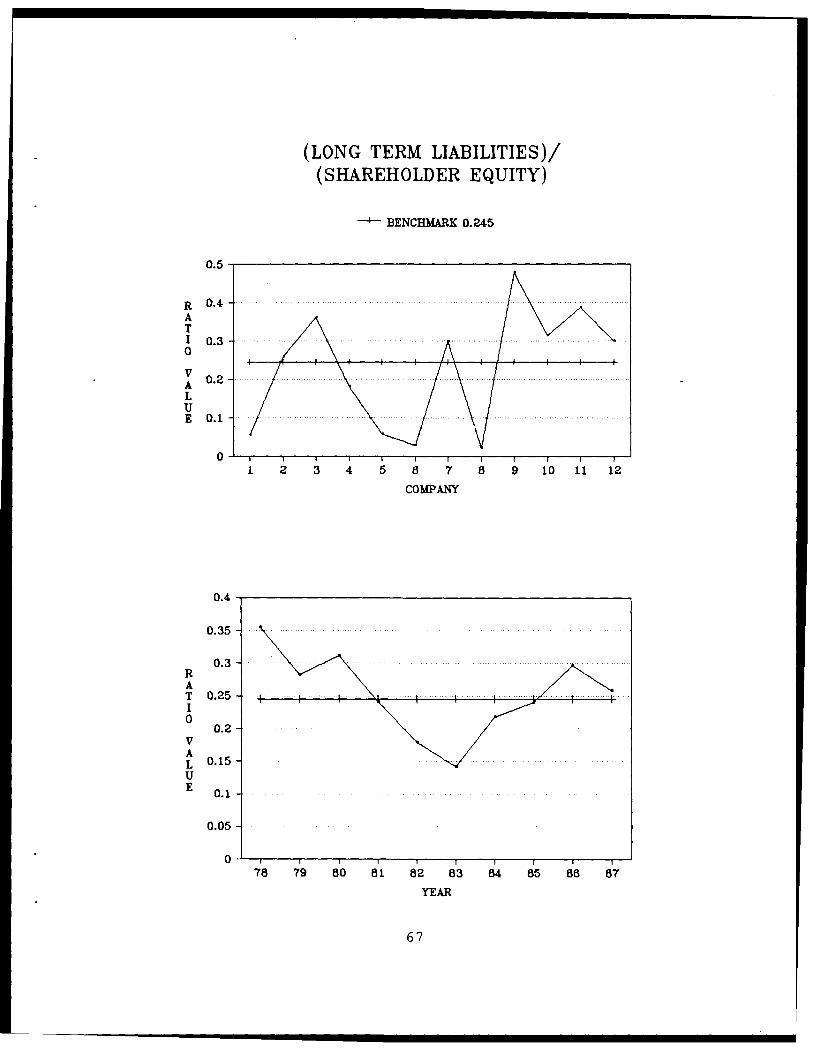
(LONG TERM LIABILITIES)/

(SHAREHOLDER EQUITY)

-- BENCHMARK 0.245

0.5-

R 0.4-AT1 0.3 -. ...0

Lu

1 2 3 4 5 5 7 B 10 11 12

COMPANY

0.4 - _ _ _ _ _ _ _ _ _ _ _ _ _ _ _ _ _ _ _ _ _ _ _ _ _ _ _ _

0.35-

0.3-

AT 0.2510

0.2-vAL 0.15-UE 0.1

0.05-

78 79 80 81 82 83 84 85 88 87

YEAR

67

(TOTAL LIABILITIES)/

(SHAREHOLDER EQUITY)

BENCHMARK 1. 053

2-

R 1 . ... ....... ..... ........ .......... ... .......ATI

0 A

AL

E

1 2 3 6 7 8 9 10 11 2

COMPANY

1.65

1.4.......................

RA 1 .2 ...... ........ ....... ...T

V 0.8-ALU 0.6-E

0.4-

0.2

0178 79 80 81 82 83 84 85 88 87

YEAR

68

(INcoME)/(INTEREST EXPENSE)

SBENCHMARK 4.074

25-

20-RAT1 15 -...0

vA 10LUE

0-1 5 8 7 8 9 110 11 12

COMPANY

7.

AT

4-0

vA 3

LUE 2 -

78 79 80 81 82 YER83 84 85 88 87

69

(CASH FLOW)/(INTEREST EXPENSE)

SBENCHMARK 6.882

40 -

R 30ATI0

20 -. . . .

ALuE10

0*1. 2 3 4 5 8 7 8 9 10 11 12

COMdPANY

10-

RATI0

VA 4-LuE

2-

78 79 8 0 811 82 8 3 84 85 86 87

YEAR

70

(INCOME) /(SALES)

--- BENCHMARK 0.04 1

0.12-

0.1-RAT 0.08-I0

0.06-

L 0.04--

E0 .0 2 -............ .

0 111 2 36 10 11 12

COMPANY

0.05-

0.04-

AT 0.03I0*

VA 0.02-LUE

0.01-

078 79 80 81 82 83 84 85 88 87

YEAR

71

(INCOME)/(TOTAL ASSETS)

--- BENCHMARK 0.081

0.14

R 0.12-AT 0.1I0

0.08-.VA 0.08LuE 0.04-

0.02 . ..

01 2 3 4 5 7 8 9 10 11 1'2

COMPANY

0.09

0.08 - ......

A 0.08 4T

0 0.05-

V 0.04ALU 0.03-E

0.02-

0.01-

7 8 79 80' 8,1 82 83 84 85 88 87

YEAR

72

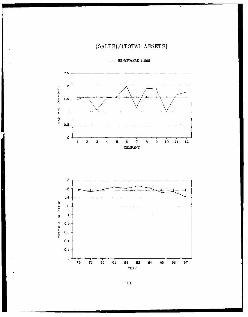
(sALES)/(TOTAL ASSETS)

-~BENCHMARK 1.565

2.5-

2-RAT1 1.50

vA 1LUE 0.5

1 2 3 9 10 1'1 1'2

COMPANY

1.85

1.4

RA 1.2-T

10 1

V 0.5ALU 0.6-E

0.4

0.2

75 79 80 81 82 83 54 85 88 87

YEAR

73

(COST OF GOODS SOLD) /(INVENTORY)

-~BENCHMARK 4.352

20-

R 15 -...AT

10-VALu 5 -... .E

0-1 2 3 4 5' 8 8 9 10 1 1,2

COMPANY

8-

RA4T

3-

ALU 2 -E

u 9 80 8 82 83 84 8 5 88 87-

YEAR

74

Appendix C: Calculated Financial Ratios

CASH + SHORT TERM INVESTMENTS / CURRENT LIABILITIES

COMPANY

YEAR 1 2 3 4 5 6

1978 0.103 0.996 0.081 0.181 0.323 0.5331979 0.094 0.836 0.056 0.145 0.171 0.3121980 0.160 0.516 0.025 0.265 0.005 0.4711981 0.132 0.283 0.017 0.322 0.006 0.2911982 0.146 0.082 0.098 0.259 0.105 0.1611983 0.035 0.342 0.176 0.263 0.153 0.0651984 0.060 0.395 0.192 0.616 0.009 0.0031985 0.373 0.727 0.007 0.185 0.020 0.0051986 0.053 0.737 0.087 0.207 0.018 0.0031987 0.101 0.486 0.085 0.209 0.011 0.002

COMPANY

YEAR 7 8 9 10 11 12

1978 0.007 0.276 0.037 0.734 0.210 0.2131979 0.036 0.312 0.044 0.628 0.067 0.1501980 0.097 0.338 0.050 0.593 0.046 0.1841981 0.603 0.401 0.034 1.158 0.058 0.1741982 0.063 0.364 0.041 1.840 0.040 0.2571983 0.797 0.425 0.087 2.052 0.069 0.1831984 0.484 0.404 0.026 0.548 0.060 0.2111985 0.737 0.136 0.008 0.165 0.236 0.4561986 0.035 0.222 0.064 0.280 0.058 0.0911987 0.116 0.276 0.038 0.547 0.091 0.055

* Companies listed alphabetically

75

CASH + SHORT TERM INVESTMENTS / TOTAL ASSETS

COMPANY

YEAR 1 2 3 4 5 6

1978 0.021 0.517 0.035 0.060 0.190 0.2801979 0.030 0.470 0.021 0.055 0.097 0.1511980 0.042 0.272 0.010 0.061 0.003 0.2521981 0.034 3.132 0.006 0.062 0.004 0.1551982 0.028 0.039 0.037 0.068 0.062 0.0921983 0.011 0.147 0.056 0.074 0.085 0.0381984 0.018 0.188 0.062 0.190 0.006 0.0021985 0.085 0.347 0.003 0.065 0.011 0.0031986 0.017 0.377 0.043 0.066 0.010 0.0021987 0.034 0.273 0.035 0.061 0.006 0.002

COMPANY

YEAR 7 8 9 10 11 12

1978 0.002 0.128 0.009 0.169 0.070 0.083

1979 0.013 0.154 0.012 0.126 0.026 0.0641980 0.019 0.167 0.010 0.093 0.020 0.0841981 0.134 0.203 0.008 0.156 0.022 0.0771982 0.228 0.175 0.009 0.223 0.015 0.1171983 0.218 0.198 0.017 0.210 0.027 0.0821984 0.136 0.196 0.006 0.071 0.023 0.077

1985 0.160 0.062 0.002 0.024 0.092 0.1391986 0.008 0.098 0.012 0.043 0.024 0.0421987 0.030 0.126 0.009 0.078 0.036 0.021

76

QUICK RATIO

COMPANY

YEAR 1 2 3 4 5 6

1978 0.874 1.228 0.998 0.950 0.492 0.9211979 0.659 1.032 1.071 0.929 0.377 0.6781980 0.824 0.676 1.116 1.346 0.214 0.6701981 0.811 0.447 1.292 1.541 0.196 0.5811982 0.748 0.235 1.148 1.100 0.303 0.3381983 0.570 0.510 1.341 1.042 0.380 0.2851984 0.547 0.587 1.378 1.224 0.257 0.2711985 0.839 0.927 0.858 0.864 0.334 0.3721986 0.463 0.949 0.957 1.132 0.358 0.3661987 0.532 0.822 1.237 1.081 0.312 0.443

COMPANY

YEAR 7 8 9 10 11 12

1978 0.963 0.878 0.767 1.528 0.883 0.8701979 0.997 0.833 0.754 1.420 0.593 0.8171980 1.434 0.814 1.090 1.496 0.544 0.8191981 1.799 0.889 0.964 2.152 0.575 0.8241982 2.172 0.885 0.817 2.679 0.549 0.7841983 1.809 0.974 0.962 2.998 0.579 0.9221984 1.459 0.940 0.668 1.731 0.610 1.0101985 1.930 0.656 0.600 1.200 0.765 1.2991986 0.998 0.721 0.851 1.204 0.595 0.5531987 1.046 0.775 0.709 1.459 0.616 0.654

77

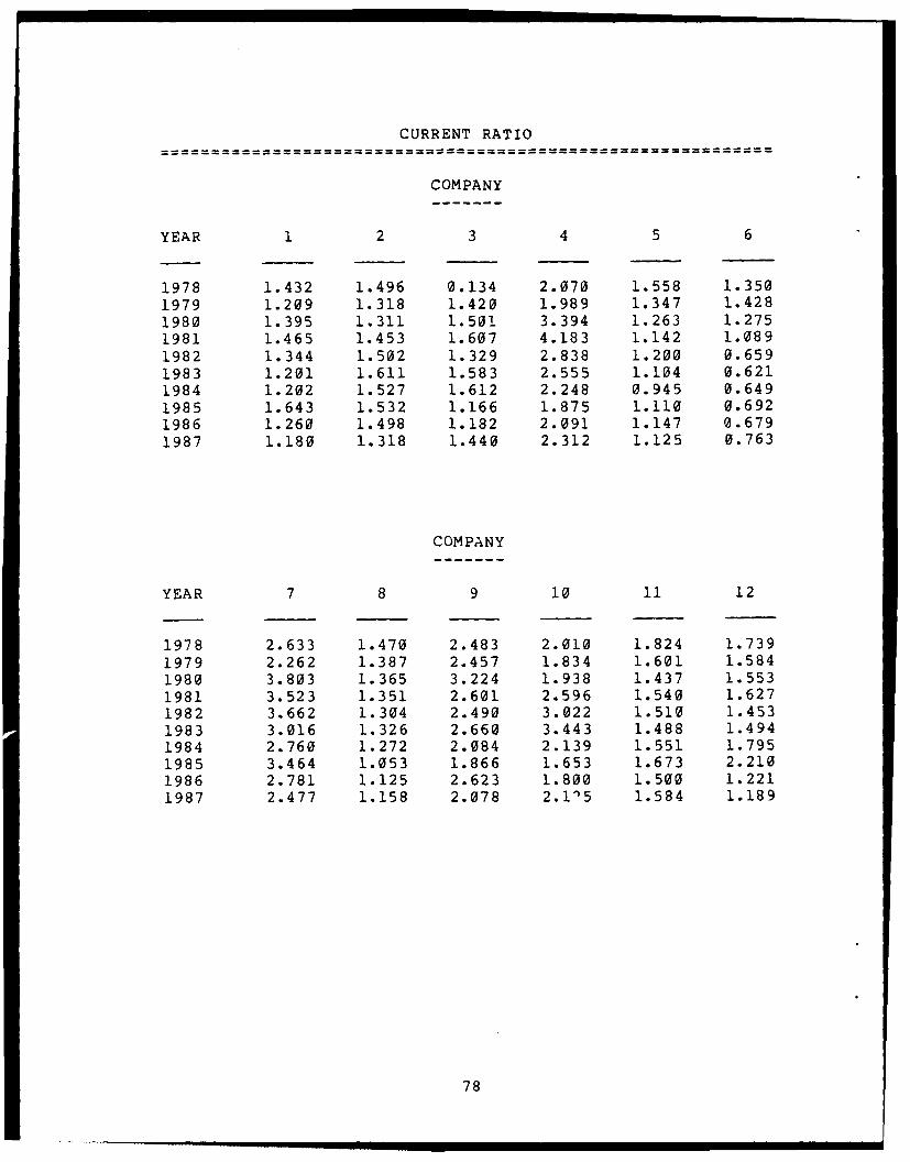
CURRENT RATIO

COMPANY

YEAR 1 2 3 4 5 6

1978 1.432 1.496 0.134 2.070 1.558 1.350

1979 1.209 1.318 1.420 1.989 1.347 1.428

1980 1.395 1.311 1.501 3.394 1.263 1.275

1981 1.465 1.453 1.607 4.183 1.142 1.089

1982 1.344 1.502 1.329 2.838 1.200 0.659

1983 1.201 1.611 1.583 2.555 1.104 0.621

1984 1.202 1.527 1.612 2.248 0.945 0.649

1985 1.643 1.532 1.166 1.875 1.110 0.692

1986 1.260 1.498 1.182 2.091 1.147 0.679

1987 1.180 1.318 1.440 2.312 1.125 0.763

COMPANY

YEAR 7 8 9 10 11 12

1978 2.633 1.470 2.483 2.010 1.824 1.739

1979 2.262 1.387 2.457 1.834 1.601 1.584

1980 3.803 1.365 3.224 1.938 1.437 1.553

1981 3.523 1.351 2.601 2.596 1.540 1.627

1982 3.662 1.304 2.490 3.022 1.510 1.453

1983 3.016 1.326 2.660 3.443 1.488 1.494

1984 2.760 1.272 2.084 2.139 1.551 1.795

1985 3.464 1.053 1.866 1.653 1.673 2.210

1986 2.781 1.125 2.623 1.800 1.500 1.221

1987 2.477 1.158 2.078 2.1'5 1.584 1.189

78

WORKING CAPITAL / SALES

COMPANY

YEAR 1 2 3 4 5 6

1978 0.000 0.169 0.060 0.148 0.159 0.0001979 0.000 0.108 0.064 0.203 0.126 0.0001980 0.000 0.103 0.071 0.290 0.100 0.0001981 0.000 0.150 0.080 0.343 0.051 0.0001982 0.000 0.199 0.061 0.242 0.075 0.0001983 0.023 0.176 0.079 0.213 0.034 -0.1071984 0.026 0.206 0.076 0.218 -0.021 -0.1061985 0.213 0.172 0.040 0.160 0.039 -0.0791986 0.081 0.173 0.046 0.198 0.050 -0.095i987 0.056 0.146 0.099 0.260 0.046 -0.080

COMPANY

YEAR 7 8 9 10 11 12

1978 0.286 0.000 0.310 0.000 0.000 0.0001979 0.303 0.131 0.315 0.124 0.000 0.0001980 0.310 0.123 0.372 0.127 0.000 0.0001981 0.318 0.128 0.334 0.189 0.115 0.0001982 0.350 0.096 0.315 0.276 0.114 0.114

1983 0.312 0.098 0.337 0.323 0.112 0.1341984 0.275 0.083 0.267 0.117 0.127 0.175

1985 0.304 0.015 0.224 0.085 0.185 0.2601986 0.226 0.035 0.289 0.103 0.148 0.1561987 0.202 0.052 0.281 0.157 0.159 0.072

79

CASH FLOW / SALES

COMPANY

YEAR 1 2 3 4 5 6

1978 0.099 0.077 0.015 0.029 0.054 0.0601979 0.093 0.079 0.070 0.029 0.052 0.0741980 0.101 0.086 0.066 0.031 0.040 0.0701981 0.108 0.078 0.049 0.023 0.043 0.0451982 0.106 0.071 0.048 0.058 0.053 0.0021983 0.092 0.065 0.064 0.065 0.060 0.031

1984 0.088 0.111 0.073 0.060 0.072 0.0451985 0.009 0.070 0.073 0.047 0.068 0.0421986 0.082 0.069 0.023 0.047 0.062 0.0071987 0.078 0.064 0.081 0.039 0.063 0.057

COMPANY

YEAR 7 8 9 10 11 12

1978 0.071 0.058 0.116 0.125 0.055 0.050

1979 0.080 0.063 0.121 0.162 0.055 0.0581980 0.046 0.063 0.127 0.144 0.052 0.0541981 0.058 0.066 0.134 0.155 0.056 0.0531982 0.060 0.070 0.124 0.126 0.057 0.0481983 0.071 0.077 0.109 0.137 0.062 0.0381984 0.080 0.086 0.123 0.195 0.067 0.045

1985 0.065 0.092 0.114 0.202 0.071 0.0361986 0.072 0.095 0.090 0.107 0.034 0.0461987 0.075 0.102 0.090 0.148 0.065 0.072

80

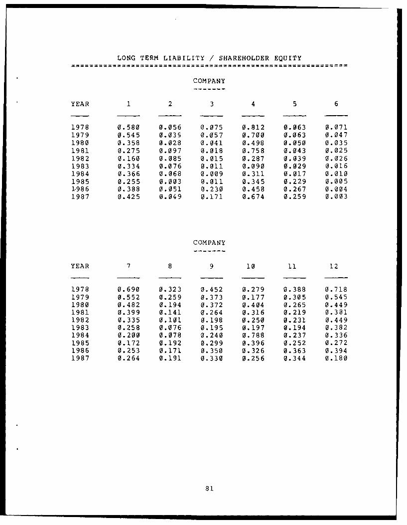
LONG TERM LIABILITY / SHAREHOLDER EQUITY

COMPANY

YEAR 1 2 3 4 5 6

1978 0.580 0.056 0.075 0.812 0.063 0.0711979 0.545 0.039 0.057 0.700 0.063 0.0471980 0.358 0.028 0.041 0.498 0.050 0.0351981 0.275 0.097 0.018 0.758 0.043 0.0251982 0.160 0.085 0.015 0.287 0.039 0.0261983 0.334 0.076 0.011 0.090 0.029 0.0161984 0.366 0.068 0.009 0.311 0.017 0.0101985 0.255 0.003 0.011 0.345 0.229 0.0051-986 0.388 0.051 0.230 0.458 0.267 0.0041987 0.425 0.049 0.171 0.674 0.259 0.003

COMPANY

YEAR 7 8 9 10 11 12

1978 0.690 0.323 0.452 0.279 0.388 0.7181979 0.552 0.259 0.373 0.177 0.305 0.5451980 0.482 0.194 0.372 0.404 0.265 0.4491981 0.399 0.141 0.264 0.316 0.219 0.3811982 0.335 0.101 0.198 0.250 0.231 0.4491983 0.258 0.076 0.195 0.197 0.194 0.3821984 0.200 0.078 0.240 0.788 0.237 0.3361985 0.172 0.192 0.299 0.396 0.252 0.2721986 0.253 0.171 0.350 0.326 0.363 0.3941987 0.264 0.191 0.330 0.256 0.344 0.180

81

rOTAL LIABILITY / SHAREHOLDER EQUITY

COMPANY

YEAR 1 2 3 4 5 6

1978 0.975 1.198 0.899 1.715 1.582 1.2541979 1.264 1.371 0.700 1.742 1.453 1.0311980 0.837 1.175 0.680 0.949 1.578 1.2261981 0.716 1.060 0.555 1.177 1.639 1.1831982 0.437 1.057 0.627 0.748 1.540 1.4061983 0.902 0.884 0.483 0.514 1.317 1.4361984 0.943 1.039 0.485 0.897 1.642 1.4371985 0.625 0.921 0.743 1.070 1.759 1.3731986 1.054 1.151 1.421 1.138 1.781 -1.7391987 1.154 1.395 1.015 1.364 1.874 1.927

COMPANY

YEAR 7 8 9 10 11 12

1978 1.399 1.467 0.937 0.661 1.087 1.8071979 1.392 1.480 0.862 0.473 1.144 1.6941980 0.855 1.367 0.717 0.665 1.238 1.6621981 0.798 1.311 0.672 0.522 0.984 1.4621982 0.699 1.124 0.511 0.423 0.990 1.6711983 0.731 1.011 0.496 0.334 0.947 1.5011984 0.670 1.088 0.624 1.054 0.992 1.0981985 0.496 1.177 0.741 0.637 1.056 0.8311986 0.626 1.102 0.652 0.564 1.339 1.6011987 0.707 1.193 0.750 0.465 1.211 0.894

82

NET INCOME / INTEREST EXPENSE

COMPANY

YEAR 1 2 3 4 5 6

1978 1.750 41.935 -2.812 1.255 23.612 24.0791979 1.718 66.500 18.309 0.738 18.478 31.3041980 2.833 54.099 6.940 1.105 9.451 29.6901981 3.053 16.538 3.496 0.374 2.530 6.3871982 2.230 6.791 4.105 2.082 8.041 1.1251983 1.883 8.452 11.794 7.175 27.490 6.5821984 1.733 21.861 57.833 4.866 5.255 21.3971985 -1.251 28.300 16.126 2.198 3.635 12.3221986 2.037 24.630 -1.059 1.446 2.731 1.4261987 1.782 17.778 8.475 0.420 2.432 1.865

COMPANY

YEAR 7 8 9 10 11 12

1978 1.514 3.675 2.710 15.685 5.128 2.8221979 1.393 4.184 3.112 29.745 2.349 3.5451980 0.463 5.582 3.063 15.987 1.509 4.1791981 1.980 5.790 3.230 15.677 1.595 5.3551982 2.620 5.149 2.829 8.253 1.483 5.4911983 5.433 9.155 1.912 10.256 2.093 1.8901984 6.242 10.133 2.623 14.322 2.503 4.0191985 4.262 6.499 1.918 21.015 2.512 5.5631986 4.525 6.314 0.806 11.624 0.170 1.1591987 4.043 7.065 0.517 23.284 1.716 1.391

83

CASH FLOW / INTEREST EXPENSE

COMPANY

YEAR 1 2 3 4 5 6

1978 4.705 54.364 2.797 2.397 32.459 29.6721979 3.921 83.987 28.208 1.590 25.629 40.5091980 5.490 72.658 11.132 1.930 15.961 40.1721981 6.096 26.717 6.946 0.820 4.562 11.9731982 5.361 14.930 7.621 2.663 14.524 1.1251983 3.841 17.143 18.864 9.384 48.620 6.5821984 3.377 32.000 86.530 6.871 11.184 21.3971985 0.372 47.600 25.762 3.822 8.155 12.3221986 3.276 41.778 3.511 2.943 7.730 1.4261987 2.983 36.444 14.686 2.029 6.470 6.834

COMPANY

YEAR 7 8 9 10 11 12

1978 2.247 5.780 4.601 19.298 7.550 3.9581979 2.029 6.199 4.739 35.135 3.561 4.7361980 1.205 8.606 4.570 19.653 2.482 5.4311981 3.288 9.171 4.768 19.129 2.654 6.8931982 4.486 8.062 4.850 11.424 2.695 7.5341983 7.647 14.631 4.295 13.697 3.740 3.0861984 8.481 16.286 5.064 16.980 4.269 5.9861985 7.183 11.392 3.755 25.319 4.175 11.4581986 8.070 12.080 2.303 16.878 1.872 4.9021987 7.373 13.729 1.830 29.290 3.252 3.359

84

NET INCOME / SALES

COMPANY

YEAR 1 2 3 4 5 6

1978 0.037 0.059 -0.015 0.015 0.039 0.0481979 0.041 0.062 0.046 0.013 0.038 0.0571980 0.052 0.064 0.041 0.018 0.024 0.0521981 0.054 0.048 0.025 0.011 0.024 0.0241982 0.044 0.032 0.026 0.045 0.029 0.0021983 0.045 0.032 0.040 0.050 0.034 0.0311984 0.045 0.076 0.049 0.042 0.034 0.0451985 -0.031 0.042 0.046 0.027 0.030 0.0421986 0.051 0.041 -0.007 0.023 0.022 0.0071987 0.046 0.031 0.047 0.008 0.024 0.016

COMPANY

YEAR 7 8 9 10 11 12

1978 0.048 0.037 0.068 0.102 0.037 0.0361979 0.055 0.042 0.080 0.137 0.036 0.0441980 0.018 0.041 0.085 0.117 0.032 0.0411981 0.035 0.041 0.091 0.127 0.033 0.0411982 0.035 0.045 0.072 0.091 0.031 0.0351983 0.050 0.048 0.049 0.102 0.035 0.0231384 0.059 0.053 0.064 0.164 0.039 0.0311985 0.038 0.053 0.058 0.168 0.042 0.0181986 0.041 0.050 0.032 0.074 0.003 0.0111987 0.041 0.052 0.025 0.117 0.034 0.030

85

NET INCOME / TOTAL ASSETS

COMPANY

YEAR 1 2 3 4 5 6

1978 0.037 0.090 -0.027 0.036 0.052 0.0951979 0.042 0.103 0.092 0.025 0.059 0.0911980 0.064 0.101 0.080 0.034 0.037 0.0701981 0.065 0.068 0.053 0.019 0.040 0.0381982 0.043 0.038 0.061 0.090 0.046 0.0041983 0.059 0.048 0.101 0.102 0.057 0.0631984 0.059 0.093 0.126 0.075 0.053 0.0851985 -0.021 0.061 0.084 0.051 0.048 0.0921986 0.054 0.060 -0.014 0.040 0.035 0.0151987 0.050 0.038 0.087 0.012 0.037 0.030

COMPANY

YEAR 7 8 9 10 11 12

1978 0.080 0.059 0.080 0.160 0.057 0.058

1979 0.080 0.063 0.095 0.183 0.051 0.0731980 0.032 0.063 0.100 0.135 0.054 0.0731981 0.062 0.061 0.106 0.144 0.061 0.0801982 0.057 0.068 0.070 0.080 0.053 0.0641983 0.089 0.074 0.048 0.079 0.058 3.0391984 0.106 0.085 0.061 0.206 0.065 0.0501985 0.067 0.081 0.057 0.198 0.060 0.0251986 0.074 0.079 0.032 0.087 0.004 0.0071987 0.078 0.073 0.023 0.120 0.050 0.029

86

SALES / TOTAL ASSETS

* COMPANY

*YEAR 1 2 3 4 5 6

1978 1.012 1.529 1.802 2.399 1.333 1.9651979 1.029 1.660 2.025 1.851 1.561 1.5981980 1.216 1.589 1.947 1.908 1.556 1.3421981 1.199 1.408 2.176 1.785 1.692 1.5831982 0.983 1.190 2.332 2.005 1.586 1.8281983 1.311 1.490 2.520 2.041 1.693 2.0431984 1.311 1.220 2.583 1.770 1.561 1.8851985 0.687 1.475 1.835 1.922 1.579 2.1681986 1.047 1.476 1.953 1.752 1.600 2.0781987 1.087 1.222 1.857 1.475 1.540 1.938

COMPANY

YEAR 7 8 9 10 11 12

1978 1.689 1.603 1.173 1.568 1.538 1.6061979 1.459 1.496 1.193 1.335 1.409 1.6701980 1.815 1.559 1.177 1.147 1.682 1.7801981 1.759 1.464 1.171 1.129 1.809 1.9281982 1.632 1.518 0.976 0.883 1.699 1.8201983 1.765 1.548 -0.992 0.773 1.682 1.6461984 1.803 1.588 0.956 1.252 1.649 1.6461985 1.753 1.546 0.979 1.177 1.424 1.4201986 1.813 1.596 1.025 1.181 1.413 0.6561987 1.896 1.387 0.923 1.026 1.439 0.990

87

COST OF GOODS SOLD / INVENTORY

COMPANY

YEAR 1 2 3 4 5 6

1978 7.545 9.066 13.056 6.158 2.144 7.464

1979 5.171 8.509 14.497 4.200 2.360 3.469

1980 6.363 3.780 11.891 3.691 2.128 3.376

1981 5.297 2.417 18.914 3.228 2.473 5.1651982 6.740 1.634 35.153 3.849 2.427 9.2181983 5.992 2.731 32.021 4.212 3.435 8.688

1984 5.661 2.293 32.438 4.948 2.941 6.8601985 3.161 4.409 12.710 4.942 2.979 9.8841986 3.567 4.472 19.287 5.341 3.057 9.4101987 4.156 3.717 20.967 3.944 2.731 8.196

COMPANY

YEAR 7 8 9 10 11 12

1978 2.450 4.741 1.859 10.453 3.689 3.951

1979 2.774 4.455 1.788 11.829 2.721 4.1281980 2.784 4.640 1.720 12.252 3.162 4.3441981 3.417 5.192 1.817 13.862 3.579 4.3601982 3.893 6.124 1.792 15.866 3.352 4.814

1983 4.131 - 7.801 1.877 13.120 3.464 5.5591984 3.910 8.103 1.829 19.444 3.328 5.139

1985 4.335 6.967 1.951 14.042 3.090 4.7531986 3.423 7.194 2.030 11.538 3.296 4.5521987 3.949 6.173 1.879 9.686 3.050 4.410

88

Bibliography

1. Bernstein, Leopold. Financial Statement Analysis:Theory, Application, and Interpretation. (ThirdEdition). Homewood IL: Irwin, 1982.

2. Bruns, William J. Jr. Introduction to Accounting,Economic Measurement for Decisions. Reading MA:Addison-Wesley, 1971.

3. Collins, R. and R. Green. "Statistical Methods forBankruptcy Forecasting," Journal of Economics andBusiness, 34: 349-354 (March 1982).

4. Deakin, E. B. "Distributions of Financial AccountingRatios: Some Empirical Evidence," The AccountingReview, 51: 90-96 (1976).

5. Derstiner, R. and R. Huefner. "LIFO-FIFO, AccountingRatios and Market Risk," Journal of AccountingResearch, 12: 216-234 (1974).

6. Dugan, Michael T. and Christine V. Zavgren. "How aBankruptcy Model Could be Incorporated as an AnalyticalProcedure," The CPA Journal, 59, No. 5: 64-65 (May1989).

7. Easton, Edison E. and Byron L. Newton. Accounting andthe Analysis of Financial Data. New York: McGraw-Hill, 1958.

8. Financial Accounting Standards Board. AccountingStandards Original Pronouncements July 1973 - June1985. 1985/86 Edition. New York: McGraw-Hill, 1986.

9. Financial Analysis Training Guide for Preaward andPostaward Financial Analyses. HQ DLA-AF FinancialServices Division Price/Cost and Financial AnalysisBranch, September 1978.

10. Foster, George. Financial Statement Analysis. (FirstEdition). Englewood Cliffs NJ: Prentice-Hall, 1978.

11. Foster, George. Financial Statement Analysis. (SecondEdition). Englewood Cliffs NJ: Prentice-Hall, 1986.

12. Gibson, Charles H. "How Industry Perceives FinancialRatios," Management Accounting, LXIII, No. 10, pp. 13-19 (April 1982).

89

13. Hamburg, Morris. Statistical Analysis for DecisionMaking. New York: Harcourt Brace Jovanovich, Inc.,1977.

14. Horwitz, Bertrand and Daniel Normolle. "Federal AgencyR&D Contract Awards and the FASB Rule for Privately-Funded R&D," The Accounting Review, 63: 414-435(1988).

15. Neter, John, William, Wasserman, and Michael H. Kutner.Applied Linear Regression Models. Homewood IL:Richard D. Irwin, Inc., 1983.

16. Newbold, Paul. Statistics for Business and Economics.(Second Edition). Englewood Cliffs NJ: Prentice-Hall,1988.

17. Niswonger, C. Rollin, CPA, PhD, LLD; and Philip E.Fess, CPA, PhD. Accounting Principles (12th Edition).Cincinnati OH: South-Western Publishing Co., 1977.

18. Parr, Joseph 0., Robert 0. Edminister, and M. BrianMcDonald. FINCAP Analysis. Washington DC: LogisticsManagement Institute, March 1979.

19. Robert Morris Associates 1988 Annual Statement Studies.Philadelphia: Robert Morris Associates, 1988.

20. Standard and Poor's Industrial Compustat. New York:Standard and Poor's Compustat Services, Inc., 1987.

21. Standard and Poor's Register of Corporations, Directorsand Executives 1988. New York: Standard and Poor'sCorporation, 1988.

22. Troy, Leo. Almanac of Business and IndustrialFinancial Ratios. (1986 Edition). Englewood CliffsNJ: Prentice-Hall, 1986.

23. Zavgren, Christine V. "The Prediction of CorporateFailure: The State of the Art," Journal of AccountingLiterature, 2: 1-38 (1983).

24. Zavgren, Christine V. and G. E. Friedman. "AreBankruptcy Prediction Models Worthwhile? AnApplication in Securities Analysis," ManagementInternational Review, 28: 34-44 (1988).

90

VITA

Captain Doreen C. Province

enlisted in the USAF

through 1979. She attended the University of North Carolina

in Charlotte from which she received the degree of Bachelor

of Science in Accounting in May 1984. Upon graduation, she

received a commission in the USAF through the OTS program.

She was assigned to Yokota AB, Japan as the base budget

officer. In January of 1988, she was assigned to the

Aeronautical Systems Division (AFSC) as a budget staff

officer at Wright-Patterson AFB, Ohio, until entering the

School of Systems and Logistics, Air Force Institute of

Technology, in May 1988.

91

UNCLASSIFIEDSECURITY CLASSIFICATION OF THIS PAGE

Form ApprovedREPORT DOCUMENTATION PAGE OMB No. 0704-0188

la. REPORT SECURITY CLASSIFICATION lb. RESTRICTIVE MARKINGS

UNCLASSIFIED2a. SECURITY CLASSIFICATION AUTHORITY 3. DISTRIBUTION /AVAILABILITY OF REPORT

Approved for public release;2b. DECLASSIFICATION/DOWNGRADING SCHEDULE distribution unlimited

4. PERFORMING ORGANIZATION REPORT NUMBER(S) 5. MONITORING ORGANIZATION REPORT NUMBER(S)

AFIT/GCA/LSY/89S-10

6a. NAME OF PERFORMING ORGANIZATION 6b. OFFICE SYMBOL 7a. NAME OF MONITORING ORGANIZATION

School of Systems and (If applicable)

Logistics I AFIT/LSQ6c. ADDRESS (City, State, and ZIP Code) 7b. ADDRESS (City, State, and ZIP Code)

Air Force Institute of TechnologyWright-Patterson AFB OH 45433-6583

8a. NAME OF FUNDING/SPONSORING 8b. OFFICE SYMBOL 9. PROCUREMENT INSTRUMENT IDENTIFICATION NUMBERORGANIZATION j (If applicable)

8-. ADDRESS (City, State, and ZIP Code) 10. SOURCE OF FUNDING NUMBERS

PROGRAM PROJECT TASK WORK UNITELEMENT NO. NO. NO ACCESSION NO.

11. TITLE (Include Security Classification)

FINANCIAL RATIO BENCHMARKS FOR DEFENSE INDUSTRY CONTRACTORS12. PERSONAL AUTHOR(S)

Doreen C. Province, B.S., Captain, USAF13a. TYPE OF REPORT 13b. TIME COVERED 14. DATE OF REPORT (Year, Month, Day) 15. PAGE COUNT

MS Thesis FROM TO 1989 September 10316. SUPPLEMENTARY NOTATION

17. COSATI CODES 18. SUBJECT TERMS (Continue on reverse if necessary and identify by block number)FIELD GROUP SUB-GROUP Variance Analysis

05 03 Normal Distribution

Indexes (Ratios)19. ABSTRACT (Continue on reverse if necessary and identify by block number)

Thesis Advisor: David S. Christensen, Captain, USAF

Assistant ProfessorDept of Systems Acq Mgt

Appoved for Iublicr lease: IAW AFR 190-1.

LARRY . EMMELHAINZ, Lt 01, USAF 11 Oct 89Director of Research and Consultation

Air Force Institute of Technology (AU)

Wright-Patterson AFO OH 45433-6583

20. DISTRIBUTION/AVAILABILITY OF ABSTRACT 21. ABSTRACT SECURITY CLASSIFICATION

rUNCLASSIFIED/UNLIMITED 0 SAME AS RPT. C1 DTIC USERS UNCLASSIFIED22a NAME OF RESPONSIBLE INDIVIDUAL 22b TESPHONE Incluge Area Code) 22c. OFFICE $YMBOL

David S. Christensen, Captain, USAF (513) 255- 4 t C5 AFIT/LSYDD Form 1473, JUN 86 Previous editions are obsolete. SECURITY CLASSIFICATION OF THIS PAGE

UNCLASSIFIED

UNCLASSIFIED

Abstract

The purpose of this study was to dcvelop and analyzefinancial ratio benchmarks of the aerospace defensecontracting industry. The study addressed four questions:(1) How should the aerospace defense industry bespecifically defined? (2) Which financial ratio benchmarksshould be provided? What information does a specific ratioprovide? (3) How are specific ratio benchmarks calculatedand tested for statistical significance? (4) What problemsresult from financial ratio analysis?

Review of the literature disclosed the capability ofdefining a specific industry using the Standard IndustryClassification System. An industry can be furtherrestricted by only including companies that have recentlycontracted with the Department of Defense. Based on theserestrictions the Compustat data bank was used to accesssample data.

From an extensive list of ratios, 14 were selectedfrom 7 main categories: (1) Cash Position, (2) Liquidity,(3) Working Capital/Cash Flow, (4) Capital Structure, (5) DebtService Coverage, (6) Profitability, and (7) Turnover.

The basic benchmark measurement was defined as themedian of the sample observations. Additionally, thecentral quartile was selected as the measurement of areasonable range. Assuming the sample is/was representativeof the industry, these measurements provided basic guidelinesfor all but one of the 14 ratios. The ratio WC/Salesdisplayed a trend which signified a potential need foradjustment.

Of the problems associated with ratio analysis, themost predominant constraint involves the use of alternativeinventory valuation methods. However, prior studies foundminimal consequences to company ranking resulted from theseinconsistent methods. Still, ratio analysis does notprovide a specific guide to action and its usefulness isdependent on the users ability to interpret its meaning.

UNCLASSIFIED