Ecole d’ete du non-lineaire 2014, Peyresq, France1

Large deviations in noise-perturbed dynamical systems2

Hugo TouchetteNational Institute for Theoretical Physics (NITheP)

Stellenbosch University, South Africa

3

Started: July 17, 2014; last compiled: August 31, 20144

Contents5

Introduction 26

1 From ordinary to stochastic differential equations 37

1.1 Ordinary differential equations (ODEs) . . . . . . . . . . . . . . . . . . . . . . . . . . 38

1.2 Stochastic differential equations (SDEs) . . . . . . . . . . . . . . . . . . . . . . . . . . 59

1.3 Exercises . . . . . . . . . . . . . . . . . . . . . . . . . . . . . . . . . . . . . . . . . . 810

1.4 Further reading . . . . . . . . . . . . . . . . . . . . . . . . . . . . . . . . . . . . . . . 1011

2 Low-noise large deviations of SDEs 1112

2.1 Path distribution . . . . . . . . . . . . . . . . . . . . . . . . . . . . . . . . . . . . . . . 1113

2.2 Laplace’s principle . . . . . . . . . . . . . . . . . . . . . . . . . . . . . . . . . . . . . 1214

2.3 Propagator large deviations . . . . . . . . . . . . . . . . . . . . . . . . . . . . . . . . . 1215

2.4 Stationary large deviations . . . . . . . . . . . . . . . . . . . . . . . . . . . . . . . . . 1416

2.5 *Escape problem . . . . . . . . . . . . . . . . . . . . . . . . . . . . . . . . . . . . . . 1617

2.6 Exercises . . . . . . . . . . . . . . . . . . . . . . . . . . . . . . . . . . . . . . . . . . 1718

2.7 Further reading . . . . . . . . . . . . . . . . . . . . . . . . . . . . . . . . . . . . . . . 1819

3 Reversible versus non-reversible systems 1920

3.1 Gradient systems . . . . . . . . . . . . . . . . . . . . . . . . . . . . . . . . . . . . . . 1921

3.2 Transversal systems . . . . . . . . . . . . . . . . . . . . . . . . . . . . . . . . . . . . . 2022

3.3 General systems . . . . . . . . . . . . . . . . . . . . . . . . . . . . . . . . . . . . . . . 2223

3.4 Exercises . . . . . . . . . . . . . . . . . . . . . . . . . . . . . . . . . . . . . . . . . . 2324

3.5 Further reading . . . . . . . . . . . . . . . . . . . . . . . . . . . . . . . . . . . . . . . 2425

Epilogue: Mountains and rivers 2526

1

Introduction27

� Dynamical system:28

Px.t/ D F.x.t// (1)

� Random perturbation or disturbance (noise):29

Px.t/ D F.x.t//„ ƒ‚ …deterministic

C "�.t/„ƒ‚…noise

"� 1 (2)

� Questions:30

ı How is the noise affecting the dynamics?31

ı What is the probability to go away from an attractor?32

ı What is the probability of reaching a point y from a point x?33

ı What is the most probable way to reach a point away from an attractor?34

ı What is the most probable trajectory going from x to y?35

� Applications:36

ı Physics: Noise-perturbed systems, diffusion, microscopic transport, nucleation, hydrodynamic37

fluctuation theory, etc.38

ı Chemistry: Stability of chemical reactions, spontaneous transformations;39

ı Engineering: Stability of structures, control under noisy conditions, queueing theory, etc.40

ı Biology: Molecular transport, molecular motors, chemical networks, etc.41

ı Sources: [vK92], [Gar85], [Jac10].42

� Plan:43

ı Learn about dynamical systems (ODEs) and noisy dynamical systems (SDEs);44

ı Study low-noise perturbations of dynamical systems (low-noise large deviation theory);45

ı Compare properties of reversible and non-reversible systems.46

ı Learn about climbing mountains and swimming rivers.47

� Some historical sources:48

ı Mathematics: Wiener (Wikipage), Freidlin and Wentzell [FW84].49

ı Physics: Einstein [Ein56], Langevin (Wikipage) [LG97], Onsager and Machlup [OM53],50

Graham [Gra89], Zwanzig [Zwa01].51

2

1. From ordinary to stochastic differential equations52

1.1. Ordinary differential equations (ODEs)53

� First-order ODE:54

Px.t/ D F.x; t/ (3)

ı Initial condition: x.0/ D x055

ı Force: F.x; t/56

ı Homogeneous: F.x; t/ D F.x/ (no explicit time dependence).57

ı Non-homogeneous: F.x; t/58

� Vector first-order ODE:59

Px.t/ D F.x; t /; x D

0B@ x1:::xn

1CA F D

0B@ F1:::Fn

1CA (4)

� Remark: Bold letters are not used thereafter for vectors; it will be clear from the context whether x60

is a vector or a scalar.61

� Example: Newton’s equation for the pendulum of length ` with friction:62

R� C P� Cg

`sin � D 0: (5)

Define x1 D � and x2 D P� . Then63

Px1 D x2

Px2 D � x2 �g

`sin x1:

(6)

� *Example: Driven pendulum:64

R� C P� Cg

`sin � D A.t/: (7)

Define x1 D � , x2 D P� , and x3 D t . Then65

Px1 D x2

Px2 D � x2 �g

`sin x1 C A.x3/

Px3 D 1:

(8)

� Remarks:66

ı An nth order ODE can be written as an n-component first-order ODE.67

ı An n-component first-order non-homogeneous ODE can be written as a .nC 1/-component68

ODE using xnC1 D t so that PxnC1 D 1.69

3

� Example: Linear ODE:70

Px D Ax: (9)

General solution:71

x.t/ D x.0/eAt : (10)

Express the initial condition x.0/ in the eigenbasis f�i ; vig of A:72

x.0/ DXi

aivi : (11)

Then73

x.t/ DXi

aie�i tvi : (12)

Classification of solutions (assuming ai > 0 for all i ):74

ı Exponentially decaying: Re�i < 075

ı Exponentially exploding: Re�i > 076

ı Pure oscillations: Re�i D 0 but Im�i ¤ 0.77

� Potential ODE:78

Px.t/ D �rU.x.t// (13)

ı Potential function: U.x/79

ı Gradient descending dynamics:80

PV .t/ D �rU.x.t//2 � 0 (14)

ı Px D 0 on critical points of U (minima, maxima, saddles) defined by rU.x/ D 0.81

� Fixed (equilibrium) points: x� such that F.x�/ D 0.82

ı Asymptotically stable: x.t/! x� as t !183

ı Locally stable: x.t/! x� for x.t/ D x� C ıx84

ı Locally unstable: x.t/ 6! x� for x.t/ D x� C ıx.85

� Linear stability around fixed point x�:86

Px D F.x/ D J.x�/.x � x�/CO.jx � x�j2/ (15)

ı Jacobian matrix:87

J.x�/ij D@Fi

@xj(16)

ı Stability determined as for linear systems above.88

� Euler scheme:89

x.t C�t/ D x.t/C F.x.t/; t/�t (17)

with x.0/ D x0. The force can be evaluated at any other point x.t 0/, t 0 2 Œt; t C �t� if F is90

continuous.91

4

1.2. Stochastic differential equations (SDEs)92

� Noisy ODE:93

Px.t/ D F.x.t//„ ƒ‚ …deterministic

C �.t/„ƒ‚…noise

(18)

� Gaussian random walk:94

Sn D

nXiD1

Xi ; Xi � N .0; �2/ iid: (19)

Then95

hSni D 0 (20)

var.Sn/ D h.Sn � hSni/2i D n�2: (21)

� Brownian motion (BM): Partition the time interval Œ0; t � into n D t=�t sub-intervals of size �t .96

Assign a Gaussian increment97

�W.i�t/ � N .0;�t/ (22)

to each sub-interval i D 1; : : : ; n and define98

W.t/ D limn!1

nXiD1

�W.i�t/: (23)

Properties:99

ı Initial value: W.0/ D 0100

ı Mean: hW.t/i D 0 for all t101

ı Variance: varW.t/ D t102

ı Independent increments:103

dW.t/ D W.t C dt/ �W.t/ � N .0; dt/ (24)

are independent Gaussian random variables.104

ı Integral of increments:105

W.t/ D

Z t

0

dW.t/: (25)

This gives meaning to (23) above.106

� Gaussian white noise: Formally,107

�.t/ DdW.t/

dt: (26)

The problem is that W.t/ is not differentiable for any t . Hence the derivative above does not make108

sense, but the increments109

dW.t/ D �.t/dt (27)

do; see properties above.110

5

� SDE:111

dX.t/ D F.X.t/; t/dt C �.Xt ; t /dW.t/ (28)

In mathematics, the time variable is usually put as a subscript:112

dXt D F.Xt ; t /dt C �.Xt ; t /dWt (29)

ı Force: F.x; t/113

ı Diffusion coefficient: �.x; t/114

ı Xt is also called a diffusion.115

� Euler-Maruyama scheme:116

XtC�t D Xt C F.Xt ; t /�t C �.Xt ; t /�Wt ; (30)

where �Wt � N .0;�t/ Dp�t N .0; 1/.117

� Vector SDE:118

dXt D F.X; t /dt C �.Xt ; t /dWt ; (31)

where119

X D

0B@X1:::Xn

1CA ; F D

0B@ F1:::Fn

1CA ; W D

0B@W1:::Wn

1CA : (32)

The Wi ’s are independent BMs. � is an n � n diffusion matrix.120

� Remark: F and � are mostly assumed here time-independent (homogeneous). For simplicity, we121

will also often assume � constant.122

� Example: Langevin equation or Ornstein-Uhlenbeck (OU) process:123

dXt D � Xtdt C �dWt ; Xt 2 R: (33)

Linear, gradient system with U.x/ D x2=2.124

� SDE convention:125

ı Ito or left-point rule:126

XtCdt D Xt C F.Xt /dt C �.Xt /dWt (34)

ı *Stratonovich or mid-point rule:127

XtCdt D Xt C F. NXt /dt C �. NXt /dWt ; NXt DXt CXtCdt

2(35)

ı *Remark: Each convention defines a Markov process to which are associated special calculus128

rules. For example, in the Ito convention,129

df .Xt / D f0.Xt /dXt C

�2

2f 00.Xt /dt (36)

for � constant, whereas in the Stratonovich convention,130

df .Xt / D f0.Xt /dXt : (37)

Thus Ito leads to a modified chain rule of calculus, which is part of Ito’s stochastic calculus,131

whereas Stratonovich retains the normal chain rule of calculus. The different calculus rules132

come from the fact that W.t/ is non-differentiable.133

6

� Propagator:134

P.x; t jx0; 0/ D P.Xt D xjX0 D x0/: (38)

Also written as Pt .x0; x/ for a homogeneous process in the mathematical literature.135

� Fokker-Planck equation:136

@

@tP.x; t jx0; 0/ D �

@

@xF.x/P.x; t jx0; 0/C

�2

2

@2

@x2P.x; t jx0; 0/ (39)

ı Linear partial differential equation137

ı Operator form:138

@

@tP.x; t jx0; 0/ D L

�P.x; t jx0; 0/ (40)

ı Fokker-Planck operator:139

L� D �@

@xF.x/C

�2

2

@2

@x2(41)

ı Current form in Rd :140@P

@tCr � J D 0 (42)

ı Fokker-Planck current:141

J D FP �D

2rP; D D ��T (43)

� Marginal distribution: P.x; t/ D P.Xt D x/142

� Remark: P.x; t/ D P.x; t jx0; 0/ for the initial condition P.x; 0/ D ı.x � x0/.143

� Stationary distribution:144

@

@tP �.x/ D L�P �.x/ D 0 (44)

� Ergodic systems:145

limt!1

P.x; t/ D P �.x/ (45)

for all initial condition.146

� *Evolution of observables:147@

@thf .Xt /i D hLf .Xt /i (46)

ı Generator:148

L D F.x/@

@xC�2

2

@2

@x2(47)

ı Adjoint generator: L D .L�/� in the sense of integration by parts; see Exercise 11.149

� Infinitesimal propagator:150

P.y; t C dt jx; t/ D P.XtCdt D yjXt D x/ D Pdt .x; y/ (48)

7

� Example: Infinitesimal propagator for BM: From (23),151

Pdt .w0jw/ D P.WtCdt D w

0jWt D w/

D1

p2�dt

e�.w0�w/2=.2dt/

D1

p2�dt

e�dw2=.2dt/

D1

p2�dt

e� Pw2dt=2 (49)

� Example: Infinitesimal propagator for general Ito SDE:152

Pdt .x0jx/ D P.XtCdt D x

0jXt D x/

D1

p2��2dt

e�Œx0�x�F.x/dt�2=.2�2dt/

D1

p2��2dt

e�Œ Px�F.x/�2dt=.2�2/ (50)

� Remark: The stationary behavior of an SDE is determined by its stationary distribution P �.x/ and153

its stationary Fokker-Planck current. If a system has zero current (reversible system with gradient154

force, for example), then the stationary distribution P �.x/ is sufficient.155

1.3. Exercises156

1. (Lyapunov stability) Prove the inequality in (14); that is, show that, for a gradient descent, U.x.t//157

decreases or stays the same with time. Discuss the consequence of this result for the stability of x.t/.158

2. (Normal system) Consider the linear systems Px D Bx. Show that x.t/! 0 exponentially fast if (i)159

ŒB; BT � D 0 (we then say that B is a normal matrix) and (ii) BCBT is negative definite. [Note: These160

are sufficient but non-necessary conditions for x.t/ to be asymptotically stable. Can you state necessary161

and sufficient conditions?]162

3. (Van der Pol oscillator) Consider the nonlinear dynamical system defined by the 2nd-order ODE163

Rx C �.x2 � 1/ Px C x D 0: (51)

(a) Write this ODE as a vector system of two first-order ODEs.164

(b) Solve this system for � D �1 using a Euler scheme or some ODE solver available, for example, in165

Matlab, Maple or Mathematica. Try different initial conditions. Plot a solution for a given initial166

condition as a function of time t . Then plot it as a phase space plot (i.e., Px vs x). What is the fixed167

point or attractor of the system?168

(c) Repeat Part (b) for � D 1.169

4. (Time-delayed ODE) Obtain a numerical solution of the following ODE:170

Px.t/ D sin�x.t � 2�/

�(52)

for t 2 Œ0; 200� and fx.t/g0tD�2� D 0:1 as the initial (function) condition. Use Euler’s scheme or the171

delayed ODE solver available in Matlab or Mathematica. Repeat for fx.t/g0tD�2� D 0:11 and display172

your two solutions on the same plot. Can you solve (52) by specifying only the initial point x.0/?173

[Note: x.t � 2�/ is x.t 0/ evaluated at the time t 0 D t � 2� .]174

8

5. (Convergence of Euler scheme) Consider the simple linear ODE175

Px.t/ D �x.t/:

Implement Euler’s scheme for this equation and study the convergence of this scheme with the integra-176

tion time-step �t by plotting on a log-log plot the maximum difference177

maxt2Œ0;T �

ˇxeuler.t/ � xexact.t/

ˇbetween Euler’s solution and the exact solution xexact.t/ D x.0/ e

�t as a function of �t . Use sensible178

values for T and �t .179

6. (Brownian motion) Prove all the properties of BM listed after (23). Show moreover that180

hW.t/W.t 0/i D minft; t 0g; (53)

and181

h�.t/�.t 0/i D ı.t � t 0/; (54)

where �.t/ is defined formally as in (27).182

7. (Langevin equation) Consider the Langevin equation of (33).183

(a) Use the Euler-Maruyama scheme to obtain and plot a few sample paths of this SDE.184

(b) Derive the full propagator P.x; t jx0; 0/ of this SDE analytically by solving the associated time-185

dependent Fokker-Planck equation (39). [Solution in [Gar85].]186

(c) Derive the stationary distribution of this SDE.187

8. (Infinitesimal propagator) Derive the infinitesimal generator (50) in both the Ito and Stratonovich188

conventions.189

9. (Gradient SDE) Prove that the stationary distribution of a gradient SDE,190

dXt D �rU.Xt /dt C �dWt ; (55)

has the form191

P.x/ D C e�2U.x/=�2

; (56)

where C is a normalization constant. What conditions on U.x/ must be imposed to have this solution?192

10. (Noisy Van der Pol oscillator) Use the Euler-Maruyama scheme to simulate the following SDE:193

Px D v

Pv D �x C v.˛ � x2 � v2/Cp" �.t/: (57)

This system is slightly different from (51): the bifurcation is now at ˛ D 0.194

11. (Generator) Show that the Fokker-Planck generator L� of (41) is the adjoint of the generator L of (47)195

with respect to the following inner product:196

hf; gi D

Z 1�1

f .x/g.x/ dx: (58)

[Hint: Use integration by parts.]197

9

1.4. Further reading198

� Bifurcations, limit cycles, chaos and applications of ODEs: [Str94].199

� ODE solvers in Matlab and Mathematica.200

� SDEs and Markov processes: [vK92], [Gar85], [Ris96], [Jac10].201

� Stochastic calculus: [Gar85], [Jac10], [BZ99].202

� Ito vs Stratonovich convention: [vK81], [Gar85].203

� Numerical integration of SDEs: [Hig01].204

� Non-white or colored noises: see Wikipage.205

10

2. Low-noise large deviations of SDEs206

2.1. Path distribution207

� Noise-perturbed dynamical system (SDE):208

dXt D F.Xt /dt Cp" � dWt ; Xt 2 R (59)

� Remark: We will deal with one-dimensional SDEs throughout the lectures; the generalization to209

Rd is the subject of Exercise 6.210

� Trajectory: fx.t/gTtD0211

� Discrete-time (sampled) trajectory: fxigniD1 with xi D x.i�t/ and n D T=�t ; see Fig. 1.212

� Joint distribution:213

P.x0; x1; : : : ; xn/ D P.x0/

n�1YiD1

P�t .xiC1jxi / (60)

� Path distribution (or density):214

P Œx� D P.fXt D xtgTtD0/ D lim

�t!0P.x0; : : : ; xn/ (61)

� Low-noise approximation:215

P Œx� � e�I Œx�=" (62)

� Action:216

I Œx� D1

2�2

Z T

0

Œ Px.t/ � F.x.t//�2dt (63)

ı Also called the dynamical action or path rate function.217

ı Non-negativity: I Œx� � 0218

ı Zero: I Œx� D 0 iff Px D F.x/219

ı Called the deterministic, noiseless, relaxation or natural path.220

� Large deviation principle (LDP):221

lim"!0�" lnP Œx� D I Œx�: (64)

This limit gives meaning to the approximation (62).222

(a)

t=0

x(t)

(b)

x(t)

t=τ

x0

x1

xn

Δt

x0

x2x

Figure 1: Sampled path.

11

� *Remark: The path density (61) does not exist rigorously speaking. Moreover, it is known that223

paths of SDEs driven by BM are non-differentiable everywhere, so the Px in the action (63) seems224

dubious.225

The proper and rigorous interpretation of the LDP was given by Freidlin and Wentzell [FW84] and226

goes as follows:227

limı!0

lim"!0�" lnP

(sup

0�t�T

jXt � xt j < ı

)D I Œx�: (65)

This means that the probability of a family of paths fXtgTtD0 of the SDE enclosed in a cylinder or228

tube of width ı around the deterministic and smooth path fxtgTtD0 is given by I Œx� in the low-noise229

limit and the limit of smaller and smaller tube. Here there is no problem with Px because fxtgTtD0 is230

continuous – it is the path followed by the tube enclosing the random paths of the SDE considered.231

Sources: [Tou09, Sec. 6.1], [FW84].232

2.2. Laplace’s principle233

� Laplace sums:234

limn!1

1

nlnXi

enai D maxiai (66)

� Asymptotic notation:235 Xi

enai � enmaxi ai (67)

Also called the principle of largest term.236

� Laplace integrals:237

limn!1

1

nlnZ�

enf .x/dx D maxx2�

f .x/ (68)

� Asymptotic notation:238 Z�

enf .a/dx � emaxx2� f .x/ (69)

Also called the Laplace or saddle-point approximation.239

2.3. Propagator large deviations240

� Path LDP:241

P Œx� � e�I Œx�=" (70)

� Path integral representation of the propagator:242

P.x; t jx0; 0/ D

Z x.t/Dx

x.0/Dx0

DŒx� P Œx� (71)

� Laplace principle:243

P.x; t jx0; 0/ D

Z x.t/Dx

x.0/Dx0

DŒx� P Œx�

�

Z x.t/Dx

x.0/Dx0

DŒx� e�I Œx�="

� e�I Œx��=" (72)

12

ı Also called a WKB or semi-classical approximation.244

ı Contraction principle: general derivation of an LDP from an LDP (here from I to V ).245

� Propagator LDP:246

P.x; t jx0; 0/ � e�V.x;t jx0;0/=" (73)

� Quasi-potential:247

V.x; t jx0; 0/ D infx.t/Wx.0/Dx0;x.t/Dx

I Œx� (74)

ı Also called the pseudo or quasi-potential or simply the rate function.248

ı Non-negativity: V.x; t jx0; 0/ � 0249

� Instanton:250

x�.t/ D arg infx.t/Wx.0/Dx0;x.t/Dx

I Œx�

V .x; t jx0; 0/ D I Œx�� (75)

ı Also called the minimum action or most probable path.251

ı Most likely path among all (exponentially) unlikely fluctuation paths from x0 to x.252

ı Determines the propagator in the low-noise limit.253

ı There may be more than one instanton (more than one solution of the variational problem254

defining the quasi-potential).255

� Euler-Lagrange (EL) equation: x�.t/ is an optimizer of I Œx� so that256

d

dt

@L

@ Px�@L

@xD 0; x.0/ D x0; x.t/ D x (76)

ı Action density or Lagrangian:257

L.x; Px/ D1

2�2. Px � F.x//2 (77)

ı Explicit EL equation:258

Rx � F.x/F 0.x/ D 0; x.0/ D x0; x.t/ D x: (78)

This is a second-order ODE with two boundary conditions.259

� Hamilton’s equations: To any Lagrangian dynamics can be associated an equivalent Hamiltonian260

dynamics.261

ı Hamiltonian:262

H.x; p/ D p � Pxp � L. Pxp; x/; p D@L

@ Pxp(79)

ı Conjugate momentum:263

p D@L

@ PxD Px � F (80)

ı Explicit Hamiltonian:264

H.x; p/ Dp2

2C pF.x/ (81)

13

ı Hamilton’s equations:265

Px D@H

@pD p C F.x/

Pp D �@H

@xD �pF 0.x/ (82)

� Two first-order ODEs.266

� Energy is conserved: PH D 0267

ı Quasi-potential:268

V.x; t jx0; 0/ D I Œx�� D

Z t

0

L.x�; Px�/dt D

Z x

x0

p�dx�; (83)

where p� is the instanton momentum.269

� Remark: The Lagrangian and Hamiltonian equations are only auxiliary dynamics for finding the270

instanton; the real dynamics is the SDE.271

� *Hamilton-Jacobi equation:272

@V

@tCH

�x;@V

@x

�D 0; (84)

where V D V.x; t jx0; 0/.273

� *Bellman’s optimality principle:274

V.x; t jx0; 0/ D infx0fV.x; t jx0; s/C V.x0; sjx0; 0/g (85)

for any intermediate times s 2 Œ0; t �.275

� Example: The Lagrangian of the Langevin equation (33) with � D 1 is276

L D1

2. Px C x/2 (86)

and leads to the EL equation277

Rx � 2x D 0: (87)

The Hamiltonian is278

H Dp2

2� px (88)

and leads instead to279

Px D p � x; Pp D px: (89)

2.4. Stationary large deviations280

� Remark: Assume that the ODE Px D F.x/ has a unique attractor located, without loss of generality,281

at x D 0. We can always translate the attractor at 0 if need be. The case of many attractors will not282

be treated in the lectures; see further reading.283

� Stationary LDP:284

P.x/ � e�V.x/=" (90)

14

� Quasi-potential:285

V.x/ D infx.t/Wx.�1/D0;x.0/Dx

I Œx� (91)

� Instanton:286

x�.t/ D arg infx.t/Wx.�1/D0;x.0/Dx

I Œx� (92)

� Remarks:287

ı The terminal conditions x.�1/ D 0 and x.0/ D x arise because we want the stationary288

distribution in the long-time limit. Thus, we should choose x.0/ on the attractor (here assumed289

to be x D 0) and x.1/ D x. By time-translation invariance of the Lagrangian (or action), this290

is equivalent to x.�1/ D 0 and x.0/ D x.291

ı *In the infinite time limit, it does not matter whether you start at the attractor or not: from any292

initial condition, the system will go to the attractor in finite time with zero action. Consequently,293

the initial condition x.�1/ D 0 above can be changed to x.�1/ D anywhere.294

ı *It can be proved more generally that295

V.x/ D inft>0

infx.0/D0;x.t/Dx

I Œx�: (93)

Thus, a priori, the stationary quasi-potential is found by minimizing over all paths going from296

the attractor to the point x of interest after a time t . However, in many cases (all cases known297

to me) the minimization selects only those paths that achieve this in infinite time.298

� Euler-Lagrange equation: Same as (76) but with terminal conditions x.�1/ D 0, x.0/ D x.299

� Hamilton’s equations: Same as (82) but with correct terminal conditions.300

� Hamilton-Jacobi equation:301

H.x; V 0.x// D 0: (94)

Explicitly:302

FV 0 C�2

2V 02 D 0: (95)

� General properties of the quasi-potential:303

ı V.x/ � 0 with equality iff x D 0 (more generally, for x on the attractor).304

ı V.x/ is continuous but not necessarily differentiable; see Exercise 9 of Sec. 3.4.305

� General properties of the instanton x�.t/:306

ı H.x�; p�/ D 0 but p� ¤ 0.307

ı Line integral:308

V.x/ D

Z x

0

p� � dx�: (96)

Note that time is absent from this representation.309

ı Interpretation: The system naturally stays at the attractor; it needs noise to be pushed away310

from it. The quasi-potential is the optimal “push” cost needed to reach x; the instanton is the311

optimal path to get there.312

15

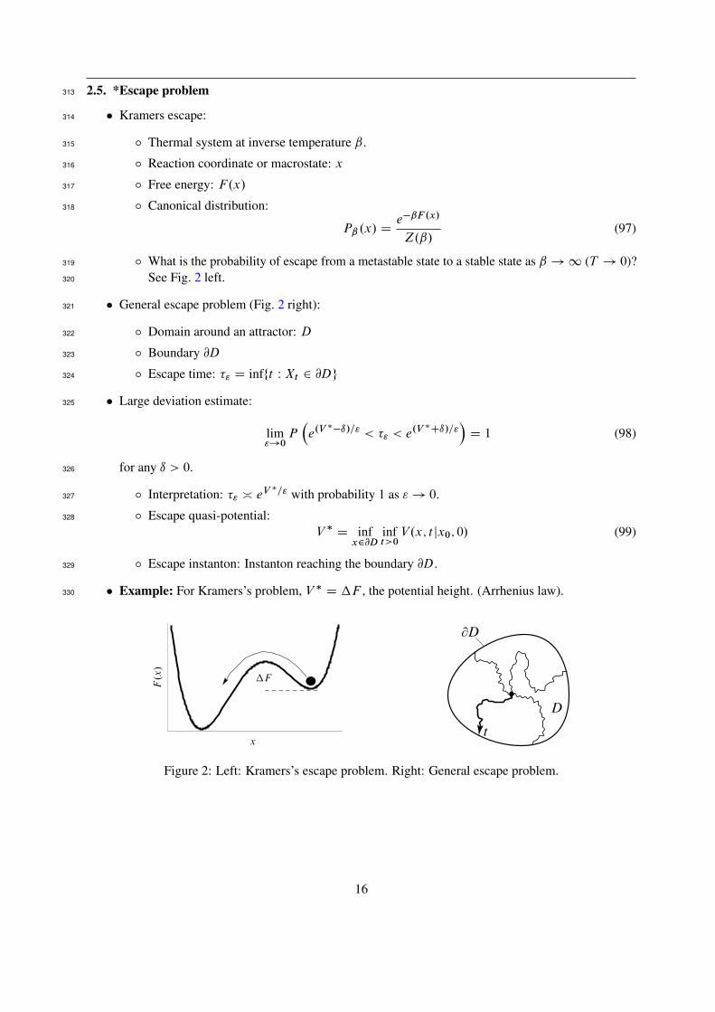
2.5. *Escape problem313

� Kramers escape:314

ı Thermal system at inverse temperature ˇ.315

ı Reaction coordinate or macrostate: x316

ı Free energy: F.x/317

ı Canonical distribution:318

Pˇ .x/ De�ˇF .x/

Z.ˇ/(97)

ı What is the probability of escape from a metastable state to a stable state as ˇ !1 (T ! 0)?319

See Fig. 2 left.320

� General escape problem (Fig. 2 right):321

ı Domain around an attractor: D322

ı Boundary @D323

ı Escape time: �" D infft W Xt 2 @Dg324

� Large deviation estimate:325

lim"!0

P�e.V��ı/=" < �" < e

.V �Cı/="�D 1 (98)

for any ı > 0.326

ı Interpretation: �" � eV�=" with probability 1 as "! 0.327

ı Escape quasi-potential:328

V � D infx2@D

inft>0

V.x; t jx0; 0/ (99)

ı Escape instanton: Instanton reaching the boundary @D.329

� Example: For Kramers’s problem, V � D �F , the potential height. (Arrhenius law).330

x

F.x

/

�F

D

∂D

t

Figure 2: Left: Kramers’s escape problem. Right: General escape problem.

16

2.6. Exercises331

1. (Laplace principle) Prove the Laplace principle for general sums, as in (66), and for general integrals,332

in as in (68). Do you need any conditions on these for approximations to be valid?333

2. (Action) Re-do the calculation of Sec. 2.1 leading to the expression of the path distribution P Œx� and334

action I Œx�. Do the calculation using first the Ito convention and then the Stratonovich convention. Are335

there any differences between the two conventions?336

3. (Hamilton equations) Show that the Hamiltonian H is conserved under Hamilton’s equations (82).337

Then show that that H.x�; p�/ D 0 for the stationary instanton. Can you find another path with zero338

energy? What differentiates this path from the instanton?339

4. (Langevin equation) Find the instanton for the quasi-potential V.x; t jx0; 0/ of the Langevin equation.340

Repeat for the stationary quasi-potential V.x/. Verify in both cases that the quasi-potentials satisfy341

their corresponding Hamilton-Jacobi equations. Finally, compare the instantons with the decay paths342

obtained by solving the corresponding noiseless ODE with the terminal conditions reversed. Do you343

see any relation between the natural paths and the instantons?344

5. (Quadratic well) Consider the vector SDE in R2 with F D �rU and345

U.x; y/ Dx2 C y2

2: (100)

Show that the natural decay path of this system satisfies the ODE Pr D �r . Then find the equation of346

the stationary instanton as well as the associated quasi-potential V.x; y/ or V.r; �/. Do you see any347

relation between the decay path and instanton? Can you write the action I Œx� in a simple form in polar348

coordinates?349

6. (Vector SDEs) Derive the action I Œx� for a set of n coupled SDEs or, equivalently, for an SDE taking350

values in Rd . Do you need any conditions on the diffusion matrix to derive the action?351

7. (Linear stream) Find the stationary quasi-potential V.x; y/ for the 2D system352

Px D BxC � (101)

with353

B D

��1 �1

1 �1

�; (102)

x D .x y/T , and � D .�x �y/T a vector of independent Gaussian white noises. Note that this a normal354

system in the sense of Exercise 2 of Sec. 1.3. Is this SDE gradient? Source: [FW84, Sec. 4.4, p. 123].355

8. (Noisy Van der Pol oscillator) Find the quasi-potential V.x; v/ of the noisy Van der Pol oscillator (57).356

[Hint: Use polar coordinates.]357

9. *(WKB approximations) Consider the following ansatz for the propagator:358

P.x; t jx0; 0/ D e�a="CbCc"Cd"2C���: (103)

(a) Use this ansatz in the Fokker-Planck equation (39) to derive the Hamilton-Jacobi equation (84).359

(b) Repeat for the stationary distribution to arrive at the Hamilton-Jacobi equation (95).360

17

10. *(Bellman’s principle) Write Bellman’s optimality principle (85) for s D t ��t and derive from the361

resulting expression the Hamilton-Jacobi equation (84). Source: [DZ98, Ex. 5.7.36, p. 237].362

11. *(Numerical instantons) Solve numerically the Euler-Lagrange equation for the Langevin equation to363

obtain V.x; t jx0; 0/ and V.x/. Repeat for Hamilton’s equations. Is there any way these equations can364

be used to avoid numerical instabilities?365

2.7. Further reading366

� Laplace principle and Laplace integrals: Chap. 6 of [BO78].367

� First work on fluctuation paths (Onsager and Machlup): [OM53].368

� Low-noise large deviations: Sec. 6.1 of [Tou09], [Gra89], Chap. 4 of [FW84] (for the mathematically369

minded), [LMD98].370

� Other large deviation limits and large deviation theory: [Ell95], [DZ98], [Tou09].371

� Escape problem: [Kra40], [HTB90], [Mel91], [Gar85].372

� Applications: [LMD98].373

� Numerical methods for finding instantons: [ERVE02], [Cam12].374

� Bellman’s optimality principle and dynamic programming: [Bel54], Wikipage, [FS06].375

18

3. Reversible versus non-reversible systems376

3.1. Gradient systems377

� SDE:378

dXt D �rU.Xt /dt Cp" �dWt ; Xt 2 Rd (104)

ı Potential: U.x/379

ı Diffusion matrix: D D ��T .380

ı Assumptions:381

1. U.x/ has a unique attractor at x D 0 corresponding to a unique minimum of U.x/.382

2. D is constant and proportional to the identity matrix.383

3. U.x/ is such that the stationary distribution exists and is unique (ergodic systems).384

� Stationary LDP:385

P.x/ � e�V.x/=" (105)

� Quasi-potential: V.x/ D 2U.x/386

Proof 1 (Direct minimization). Assume D D 11 without loss of generality. Then for any path387

fxtgTtD0 we have388

I Œx� D1

2

Z T

0

j Px CrU j2dt

D1

2

Z T

0

j Px � rU j2dt C 2

Z T

0

Px � rU dt

D1

2

Z T

0

j Px � rU j2dt C 2

Z T

0

rU � dx

� 2ŒU.xT / � U.x0/�: (106)

Thus I Œx� � 2U.x/ if x0 D 0 and ends at xT D x. The minimum is achieved for Px D rU which389

links these two points in infinite time.390

� Remark: For finite time I Œx� > 2U.x/, which means that V.x; t j0; 0/ > V.x/.391

Proof 2 (Hamilton’s equations). The instanton is such that H D 0 and p ¤ 0. This implies392

p D 2rU from (81), so that, from (96),393

V.x/ D

Z x

0

p� � dx� D 2

Z x

0

rU � dx D 2U.x/: (107)

394

� Natural dynamics or decay path:395

Pxdecay D �rU.xdecay/; xdecay.0/ D x (108)

ı Pure, dissipative hill-descent dynamics.396

ı First-order ODE.397

19

x

y

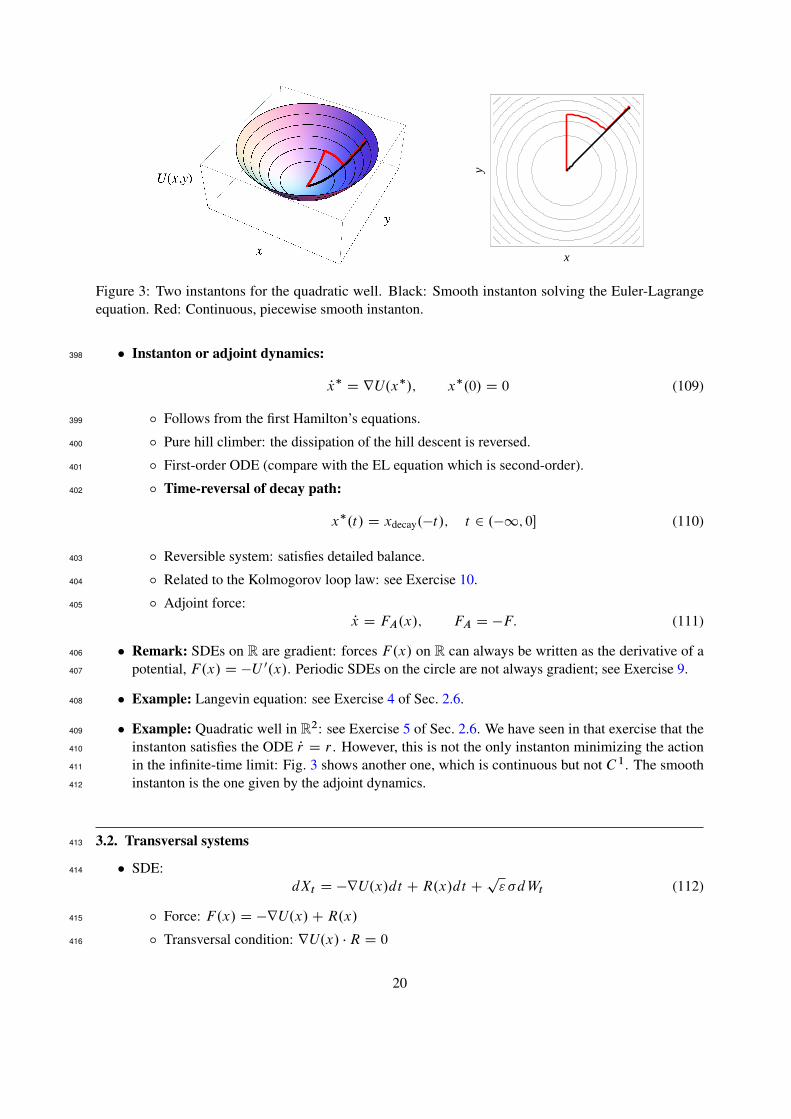
Figure 3: Two instantons for the quadratic well. Black: Smooth instanton solving the Euler-Lagrangeequation. Red: Continuous, piecewise smooth instanton.

� Instanton or adjoint dynamics:398

Px� D rU.x�/; x�.0/ D 0 (109)

ı Follows from the first Hamilton’s equations.399

ı Pure hill climber: the dissipation of the hill descent is reversed.400

ı First-order ODE (compare with the EL equation which is second-order).401

ı Time-reversal of decay path:402

x�.t/ D xdecay.�t /; t 2 .�1; 0� (110)

ı Reversible system: satisfies detailed balance.403

ı Related to the Kolmogorov loop law: see Exercise 10.404

ı Adjoint force:405

Px D FA.x/; FA D �F: (111)

� Remark: SDEs on R are gradient: forces F.x/ on R can always be written as the derivative of a406

potential, F.x/ D �U 0.x/. Periodic SDEs on the circle are not always gradient; see Exercise 9.407

� Example: Langevin equation: see Exercise 4 of Sec. 2.6.408

� Example: Quadratic well in R2: see Exercise 5 of Sec. 2.6. We have seen in that exercise that the409

instanton satisfies the ODE Pr D r . However, this is not the only instanton minimizing the action410

in the infinite-time limit: Fig. 3 shows another one, which is continuous but not C 1. The smooth411

instanton is the one given by the adjoint dynamics.412

3.2. Transversal systems413

� SDE:414

dXt D �rU.x/dt CR.x/dt Cp" �dWt (112)

ı Force: F.x/ D �rU.x/CR.x/415

ı Transversal condition: rU.x/ �R D 0416

20

-1.0 -0.5 0.0 0.5 1.0

-1.0

-0.5

0.0

0.5

1.0

-1.0 -0.5 0.0 0.5 1.0-1.0

-0.5

0.0

0.5

1.0

-1.0 -0.5 0.0 0.5 1.0-1.0

-0.5

0.0

0.5

1.0

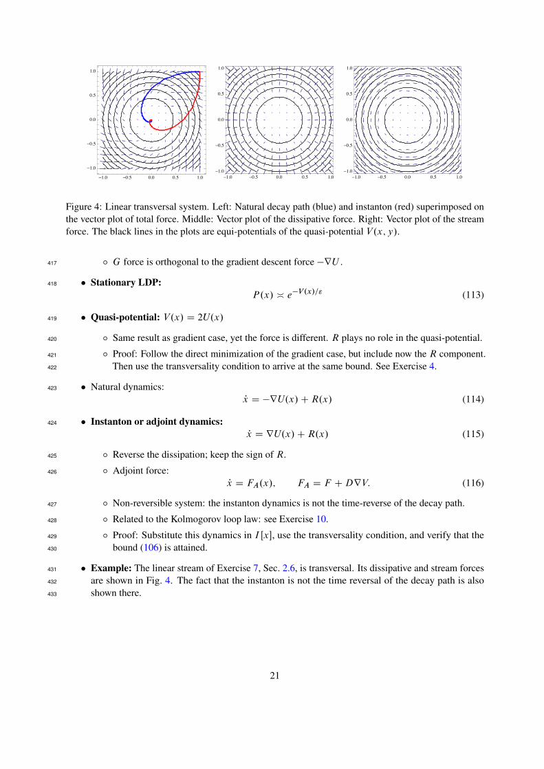
Figure 4: Linear transversal system. Left: Natural decay path (blue) and instanton (red) superimposed onthe vector plot of total force. Middle: Vector plot of the dissipative force. Right: Vector plot of the streamforce. The black lines in the plots are equi-potentials of the quasi-potential V.x; y/.

ı G force is orthogonal to the gradient descent force �rU .417

� Stationary LDP:418

P.x/ � e�V.x/=" (113)

� Quasi-potential: V.x/ D 2U.x/419

ı Same result as gradient case, yet the force is different. R plays no role in the quasi-potential.420

ı Proof: Follow the direct minimization of the gradient case, but include now the R component.421

Then use the transversality condition to arrive at the same bound. See Exercise 4.422

� Natural dynamics:423

Px D �rU.x/CR.x/ (114)

� Instanton or adjoint dynamics:424

Px D rU.x/CR.x/ (115)

ı Reverse the dissipation; keep the sign of R.425

ı Adjoint force:426

Px D FA.x/; FA D F CDrV: (116)

ı Non-reversible system: the instanton dynamics is not the time-reverse of the decay path.427

ı Related to the Kolmogorov loop law: see Exercise 10.428

ı Proof: Substitute this dynamics in I Œx�, use the transversality condition, and verify that the429

bound (106) is attained.430

� Example: The linear stream of Exercise 7, Sec. 2.6, is transversal. Its dissipative and stream forces431

are shown in Fig. 4. The fact that the instanton is not the time reversal of the decay path is also432

shown there.433

21

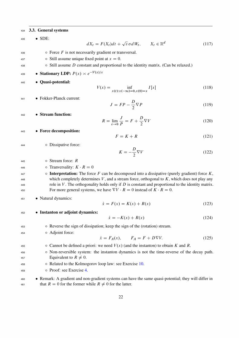
3.3. General systems434

� SDE:435

dXt D F.Xt /dt Cp" �dWt ; Xt 2 Rd (117)

ı Force F is not necessarily gradient or transversal.436

ı Still assume unique fixed point at x D 0.437

ı Still assume D constant and proportional to the identity matrix. (Can be relaxed.)438

� Stationary LDP: P.x/ � e�V.x/="439

� Quasi-potential:440

V.x/ D infx.t/Wx.�1/D0;x.0/Dx

I Œx� (118)

� Fokker-Planck current:441

J D FP �D

2rP (119)

� Stream function:442

R D lim"!0

J

PD F C

D

2rV (120)

� Force decomposition:443

F D K CR (121)

ı Dissipative force:444

K D �D

2rV (122)

ı Stream force: R445

ı Tranversality: K �R D 0446

ı Interpretation: The force F can be decomposed into a dissipative (purely gradient) force K,447

which completely determines V , and a stream force, orthogonal to K, which does not play any448

role in V . The orthogonality holds only if D is constant and proportional to the identity matrix.449

For more general systems, we have rV �R D 0 instead of K �R D 0.450

� Natural dynamics:451

Px D F.x/ D K.x/CR.x/ (123)

� Instanton or adjoint dynamics:452

Px D �K.x/CR.x/ (124)

ı Reverse the sign of dissipation; keep the sign of the (rotation) stream.453

ı Adjoint force:454

Px D FA.x/; FA D F CDrV: (125)

ı Cannot be defined a priori: we need V.x/ (and the instanton) to obtain K and R.455

ı Non-reversible system: the instanton dynamics is not the time-reverse of the decay path.456

Equivalent to R ¤ 0.457

ı Related to the Kolmogorov loop law: see Exercise 10.458

ı Proof: see Exercise 4.459

� Remark: A gradient and non-gradient systems can have the same quasi-potential; they will differ in460

that R D 0 for the former while R ¤ 0 for the latter.461

22

3.4. Exercises462

1. (Noisy Van der Pol oscillator) Consider again the noisy Van der Pol oscillator (Exercise 8, Sec. 2.6).463

Find the stream force of this system. Then find a different SDE having the same quasi-potential as this464

system, but with a null stream force, K D 0.465

2. (Three well system) Consider the gradient SDE with potential466

U.x; y/ D 3e�x2�.y�1=3/2

� 3e�x2�.y�5=3/2

�5e�.x�1/2�y2

� 5e�.xC1/2�y2

Cx4 C .y � 1=3/2

5: (126)

Find all the critical points of this potential, including the two minima at .˙1; 0/ and the shallow467

minimum at .0; 1:5/. Determine whether the instanton connecting the two deep minima goes via the468

shallow minimum or via the saddle-point between them. Source: [MSVE06].469

3. (Time reversibility) Show for a gradient system that the instanton is the time reversal of the natural470

decay path.471

4. (Transversal systems) Prove that V D 2U for transversal systems using the WKB approximation of472

Exercise 9 of Sec. 2.6 or the Hamilton-Jacobi equation. Then adapt your proof to cover the general473

systems described in Sec. 3.3.474

5. (General diffusion) Re-derive all the results of this section for a general invertible diffusion matrix D.475

That is, do not assume, as done before, that D is constant or proportional to the identity matrix. What476

happens to the whole formalism if D is not invertible?477

6. (State-dependent diffusion) Show that an SDE with gradient force F D �rU is not reversible in478

general if it has a state-dependent diffusion matrix D.x/. What can we say in general about the479

quasi-potential of such a system?480

7. (Maier-Stein system [MS93]) Consider the 2D SDE481

Px D x � x3 � ˛xy2 C �x

Py D �y � x2y C �y ; (127)

where �x and �y are two independent Gaussian white noises.482

(a) Find and classify the fixed points (stable, unstable, saddles) of the noiseless system.483

(b) Show that this system is gradient iff ˛ D 1. For this case, find the force potential U and the484

quasi-potential V . Analyze these functions in view of the fixed points found in (a).485

8. (Maier-Stein-Graham system [Gra95]) Consider the following simplification of the system above:486

Px D x � x3 C �x

Py D y � y3 � 2x2y C �y ; (128)

in which the x motion is decoupled from the y motion.487

(a) Find and classify the fixed points (stable, unstable, saddles) of the noiseless system.488

(b) Is this system gradient?489

23

(c) Find the quasi-potential V.x; y/ of the system, as well as the dissipative function K.x; y/ and490

stream function R.x; y/. The analyze these functions.491

(d) Analyze the dynamics of the instantons for points inside and outside the strip y2 D 1.492

9. *(Diffusion on the circle) Consider the following diffusion on the circle (or ring):493

d�t D Œ � U0.�t /�dt C dWt ; �t 2 Œ0; 2�/; (129)

where U.�/ D U0 cos � , U0 and are real numbers, and Wt is a normal BM. Simulate this SDE to494

understand the role of and U . Is this system gradient? Derive its stationary quasi-potential V.�/.495

Show that V D 2U iff D 0. Source: [Gra95].496

10. *(Kolmogorov loop law) Consider a path fxtgTtD0 of a Markov system and the time-reversal fxRgTtD0497

of this path defined by498

xR.t/ D x.T � t /: (130)

The Kolmogorov loop law or Kolmogorov criterion asserts that this system is reversible (in the sense of499

detailed balance) iff P Œx� D P ŒxR� for all loop paths, that is, all paths ending at their starting point.500

Use this result to show that, for reversible systems, the instanton is the time reverse of the decay path.501

Then prove that, for non-reversible systems, the instanton cannot be the time reverse of the decay path.502

11. *(Potential function) Consider a ‘loop’ sequence of states x1; x2; : : : ; xn that finishes with the starting503

state, xn D x1, and a certain function g.x; y/ of two variables. Prove that, if504

G.x1; : : : ; xn/ WDn�1XiD1

g.xi ; xiC1/ D 0 (131)

for all loop sequences, then there exists a ‘potential’ function G.x/ such that g.x; y/ D G.x/ �G.y/,505

and506

G.x1; : : : ; xn/ D G.xn/ �G.x1/ (132)

for non-loop sequences. Can you think of a differential analog of this result? What is the relation with507

the previous exercise? Is the cost of climbing a mountain potential-like?508

3.5. Further reading509

� Instanton and adjoint dynamics: [Gra95].510

� Other examples: [Gra89], [Cam12].511

� Applications: [LMD98], [LM97].512

� Time-reversibility: [OM53], [LMD98], [LM97].513

� Kolmogorov loop law: See Wikipage.514

� Many attractors: Sec. 7.14 of [Gra89], [Gra95].515

� Quasi-potential of general 2D non-reversible systems: [Cam12].516

� *Large deviation for stochastic PDEs: [FJL82], [BSGC07].517

24

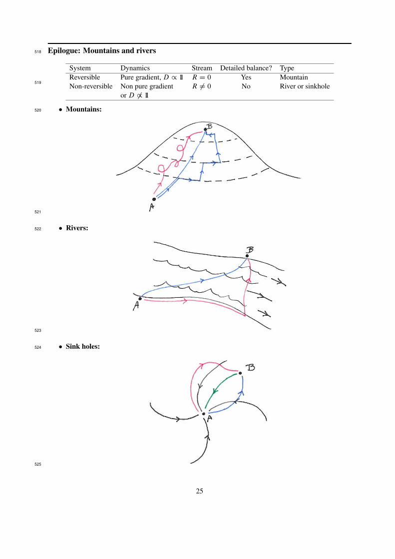
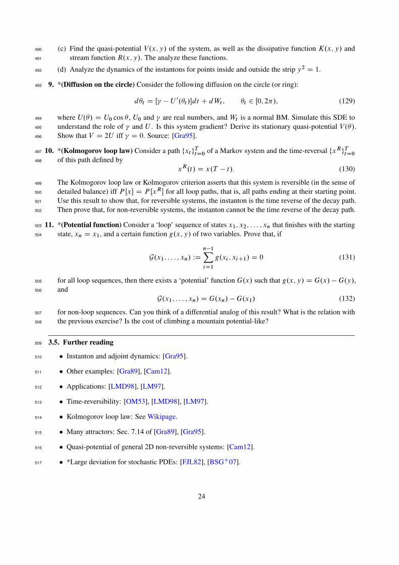
Epilogue: Mountains and rivers518

System Dynamics Stream Detailed balance? TypeReversible Pure gradient, D / 11 R D 0 Yes MountainNon-reversible Non pure gradient R ¤ 0 No River or sinkhole

or D 6/ 11

519

� Mountains:520

521

� Rivers:522

523

� Sink holes:524

525

25

References526

[Bel54] R. Bellman. The theory of dynamic programming. Bull. Am. Math. Soc.,527

60:503–515, 1954. Available from: http://www.ams.org/bull/1954-60-06/528

S0002-9904-1954-09848-8/.529

[BO78] C. M. Bender and S. A. Orszag. Advanced Mathematical Methods for Scientists and Engineers.530

McGraw-Hill, New York, 1978.531

[BSGC07] L. Bertini, A. De Sole, D. Gabrielli, G. Jona-Lasinio, and C. Landim. Stochastic interacting532

particle systems out of equilibrium. J. Stat. Mech., 2007(07):P07014, 2007. Available from:533

http://stacks.iop.org/1742-5468/2007/P07014.534

[BZ99] Z. Brzezniak and T. Zastawniak. Basic Stochastic Processes. Springer Undergraduate535

Mathematics Series. Springer, New York, 1999.536

[Cam12] M. K. Cameron. Finding the quasipotential for nongradient SDEs. Physica D, 241(18):1532–537

1550, 2012. Available from: http://www.sciencedirect.com/science/article/pii/538

S0167278912001637.539

[DZ98] A. Dembo and O. Zeitouni. Large Deviations Techniques and Applications. Springer, New540

York, 2nd edition, 1998.541

[Ein56] A. Einstein. Investigations of the Theory of Brownian Movement. Dover, New York, 1956.542

[Ell95] R. S. Ellis. An overview of the theory of large deviations and applications to statistical543

mechanics. Scand. Actuarial J., 1:97–142, 1995. Available from: http://www.math.umass.544

edu/˜rsellis/pdf-files/overview.pdf.545

[ERVE02] W. E, W. Ren, and E. Vanden-Eijnden. String method for the study of rare events. Phys.546

Rev. B, 66(5):052301, 2002. Available from: http://dx.doi.org/10.1103/PhysRevB.547

66.052301.548

[FJL82] W. G. Faris and G. Jona-Lasinio. Large fluctuations for a nonlinear heat equation with noise.549

J. Phys. A: Math. Gen., 15(10):3025, 1982. Available from: http://stacks.iop.org/550

0305-4470/15/i=10/a=011.551

[FS06] W. H. Fleming and H. M. Soner. Controlled Markov Processes And Viscosity Solutions,552

volume 25 of Stochastic Modelling and Applied Probability. Springer, New York, 2006.553

[FW84] M. I. Freidlin and A. D. Wentzell. Random Perturbations of Dynamical Systems, vol-554

ume 260 of Grundlehren der Mathematischen Wissenschaften. Springer, New York,555

1984. Available from: http://www.springer.com/mathematics/probability/book/556

978-3-642-25846-6.557

[Gar85] C. W. Gardiner. Handbook of Stochastic Methods for Physics, Chemistry and the Natural558

Sciences, volume 13 of Springer Series in Synergetics. Springer, New York, 2nd edition, 1985.559

[Gra89] R. Graham. Macroscopic potentials, bifurcations and noise in dissipative systems. In560

F. Moss and P. V. E. McClintock, editors, Noise in Nonlinear Dynamical Systems,561

volume 1, pages 225–278, Cambridge, 1989. Cambridge University Press. Available562

from: http://ebooks.cambridge.org/chapter.jsf?bid=CBO9780511897818&cid=563

CBO9780511897818A045.564

26

[Gra95] R. Graham. Fluctuations in the steady state. In J. J. Brey, J. Marro, J. M. Rubı, and M. San565

Miguel, editors, 25 Years of Non-Equilibrium Statistical Mechanics, pages 125–134, New York,566

1995. Springer. Available from: http://dx.doi.org/10.1007/3-540-59158-3_38.567

[Hig01] D. J. Higham. An algorithmic introduction to numerical simulation of stochastic differential568

equations. SIAM Review, 43(3):525–546, 2001. Available from: http://www.jstor.org/569

stable/3649798.570

[HTB90] P. Hanggi, P. Talkner, and M. Borkovec. Reaction-rate theory: Fifty years after Kramers. Rev.571

Mod. Phys., 62:251–341, 1990. Available from: http://link.aps.org/doi/10.1103/572

RevModPhys.62.251.573

[Jac10] K. Jacobs. Stochastic Processes for Physicists: Understanding Noisy Systems. Cambridge574

University Press, Cambridge, 2010.575

[Kra40] H. A. Kramers. Brownian motion in a field of force and the diffusion model of chemical576

reactions. Physica, 7(4):284–304, 1940. Available from: http://www.sciencedirect.577

com/science/article/pii/S0031891440900982.578

[LG97] D. S. Lemons and A. Gythiel. Paul Langevin’s 1908 paper “On the Theory of Brownian579

Motion” [“sur la theorie du mouvement brownien,” C. R. Acad. Sci. (Paris) 146, 530–533580

(1908)]. Am. J. Phys., 65(11):1079–1081, 1997. Available from: http://scitation.aip.581

org/content/aapt/journal/ajp/65/11/10.1119/1.18725.582

[LM97] D. G. Luchinsky and P. V. E. McClintock. Irreversibility of classical fluctuations studied583

in analogue electrical circuits. Nature, 389(6650):463–466, 1997. Available from: http:584

//dx.doi.org/10.1038/38963.585

[LMD98] D. G. Luchinsky, P. V. E. McClintock, and M. I. Dykman. Analogue studies of nonlinear586

systems. Rep. Prog. Phys., 61(8):889–997, 1998. Available from: http://stacks.iop.587

org/0034-4885/61/889.588

[Mel91] V. I. Mel’nikov. The Kramers problem: Fifty years of development. Phys. Rep., 209(1–2):1–71,589

12 1991. Available from: http://www.sciencedirect.com/science/article/pii/590

037015739190108X.591

[MS93] R. S. Maier and D. L. Stein. Escape problem for irreversible systems. Phys. Rev. E, 48(2):931–592

938, 1993. Available from: http://dx.doi.org/10.1103/PhysRevE.48.931.593

[MSVE06] P. Metzner, C. Schutte, and E. Vanden Eijnden. Illustration of transition path theory on594

a collection of simple examples. J. Chem. Phys., 125(8):084110, 2006. Available from:595

http://link.aip.org/link/?JCP/125/084110/1.596

[OM53] L. Onsager and S. Machlup. Fluctuations and irreversible processes. Phys. Rev., 91(6):1505–597

1512, 1953. Available from: http://dx.doi.org/10.1103/PhysRev.91.1505.598

[Ris96] H. Risken. The Fokker-Planck equation: Methods of solution and applications. Springer,599

Berlin, 3rd edition, 1996. Available from: http://books.google.co.uk/books?600

hl=en&lr=&id=MG2V9vTgSgEC&oi=fnd&pg=PA1&dq=risken&ots=dXVCcilAD-&sig=601

5B2cslOPyHXgNRvD4eTODTm1c-Y#v=onepage&q&f=false.602

[Str94] S. H. Strogatz. Nonlinear Dynamics and Chaos. Addison-Wesley, Reading, MAS, 1994.603

Available from: http://www.westviewpress.com/book.php?isbn=9780813349107.604

27

[Tou09] H. Touchette. The large deviation approach to statistical mechanics. Phys. Rep., 478(1-3):1–69,605

2009. Available from: http://dx.doi.org/10.1016/j.physrep.2009.05.002.606

[vK81] N. G. van Kampen. Ito versus Stratonovich. J. Stat. Phys., 24(1):175–187, 1981. Available607

from: http://dx.doi.org/10.1007/BF01007642.608

[vK92] N. G. van Kampen. Stochastic Processes in Physics and Chemistry. North-Holland, Amster-609

dam, 1992.610

[Zwa01] R. Zwanzig. Nonequilibrium Statistical Mechanics. Oxford University Press, Oxford, 2001.611

28