-core with = 2; (d) the - nature · core-periphery structures. di erent cores identi ed through...

Articulation point

Collective influence

Node degree

Model network

Technological

Infrastructure

Biological

Communication

Social (online)

A-1 A-2 A-3 A-4

B-1 B-2 B-3 C-1

C-2 C-3 D-1 D-2

E-1 E-2 E-3 F-1

F-2 F-3 F-4 F-5

Supplementary Figure 1. Comparison of different network destruction strategies in reducing the

size of the giant connected component for both model networks (A) and real-world networks (B-

F). For model networks, the data points and error bars (defined as s.e.m.) are determined from 32

independent network instances of size N = 105. The real-world networks used in this figure are:

openflights (B-1), RoadNet-TX (B-2), PG-WestState (B-3), nd.edu (C-1), oregon2-010331 (C-

2), p2p-Gnutella31 (C-3), Caenorhabditis elegans (D-1), Homo sapiens (D-2), Cellphone (E-1),

Email-Enron (E-2), UCIonline (E-3), Epinions (F-1), Slashdot-1 (F-2), Twitter (F-3), WikiVote

(F-4), Youtube (F-5) (see Supplementary Note 7 for details of the real-world networks).

1

0

0.2

0.4

0.6

0.8

1

GAPR

APTA

overlap

Model network Real-world network

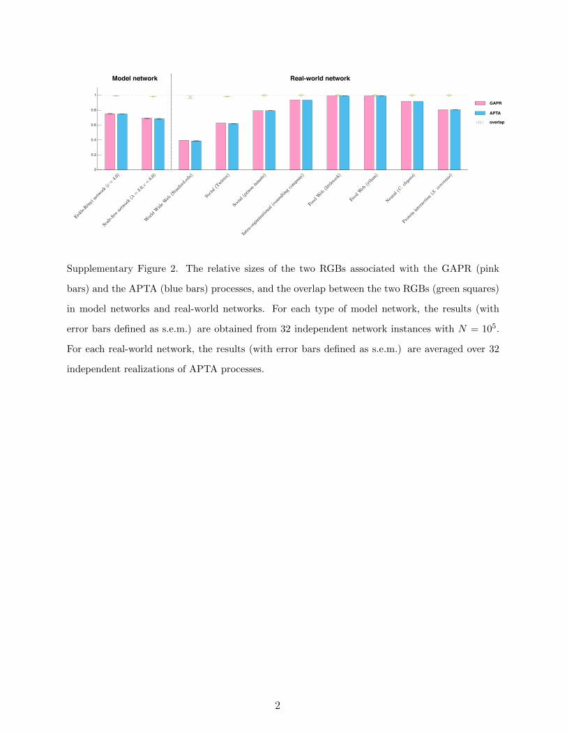
Supplementary Figure 2. The relative sizes of the two RGBs associated with the GAPR (pink

bars) and the APTA (blue bars) processes, and the overlap between the two RGBs (green squares)

in model networks and real-world networks. For each type of model network, the results (with

error bars defined as s.e.m.) are obtained from 32 independent network instances with N = 105.

For each real-world network, the results (with error bars defined as s.e.m.) are averaged over 32

independent realizations of APTA processes.

2

A B C D E F

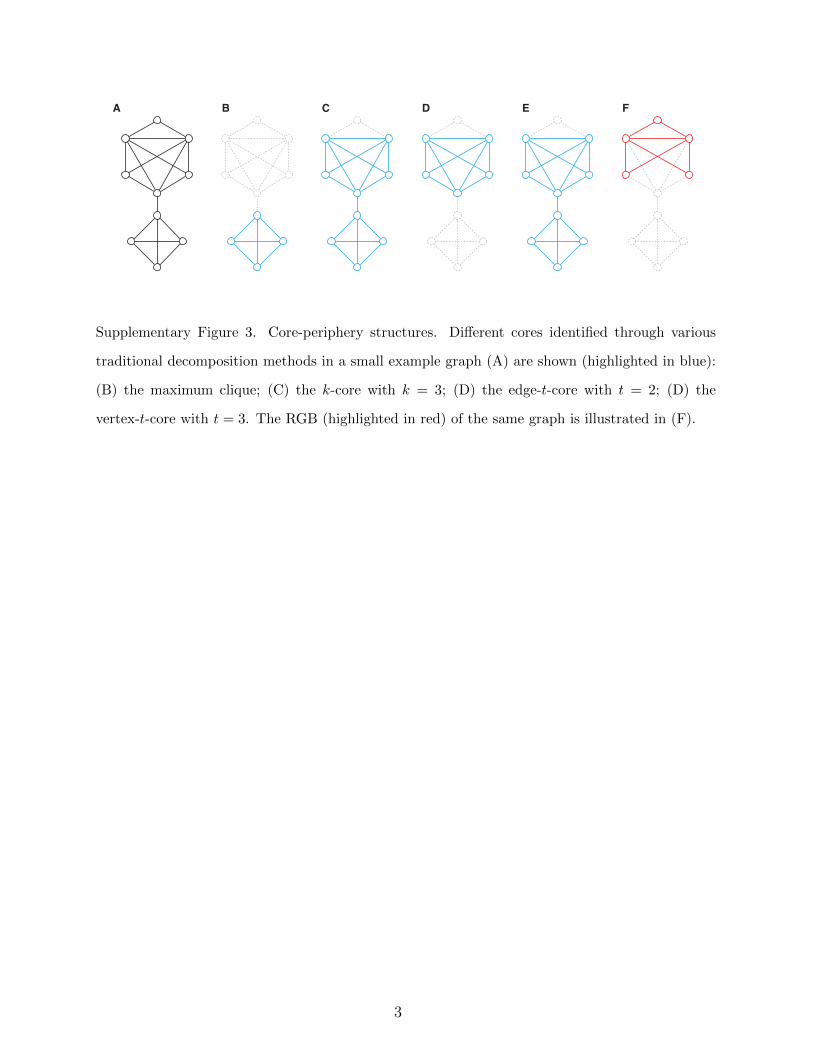
Supplementary Figure 3. Core-periphery structures. Different cores identified through various

traditional decomposition methods in a small example graph (A) are shown (highlighted in blue):

(B) the maximum clique; (C) the k-core with k = 3; (D) the edge-t-core with t = 2; (D) the

vertex-t-core with t = 3. The RGB (highlighted in red) of the same graph is illustrated in (F).

3

A B

C D

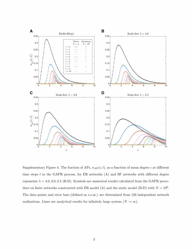
Supplementary Figure 4. The fraction of APs, nAP(c, t), as a function of mean degree c at different

time steps t in the GAPR process, for ER networks (A) and SF networks with different degree

exponents λ = 4.0, 3.0, 2.5 (B-D). Symbols are numerical results calculated from the GAPR proce-

dure on finite networks constructed with ER model (A) and the static model (B-D) with N = 106.

The data points and error bars (defined as s.e.m.) are determined from 128 independent network

realizations. Lines are analytical results for infinitely large system (N →∞).

4

Ordinary percolation

RGB percolation

GCC percolation

A B

C D

Supplementary Figure 5. The relative size of the GCC, nGCC(c, t), as a function of mean degree c

at different time steps t in the GAPR process, for ER networks (A) and SF networks with different

degree exponents λ = 4.0, 3.0, 2.5 (B-D). Symbols are numerical results calculated by performing a

given steps of GAPR procedure on finite networks constructed with ER model (A) and the static

model (B-D) with N = 106. The data points and error bars (defined as s.e.m.) are determined

from 128 independent network realizations. Thin lines are analytical results for nGCC(c, t) with

finite t, and thick lines are analytical results for the relative size of the RGB, which is nGCC(c,∞).

5

A

DC

B

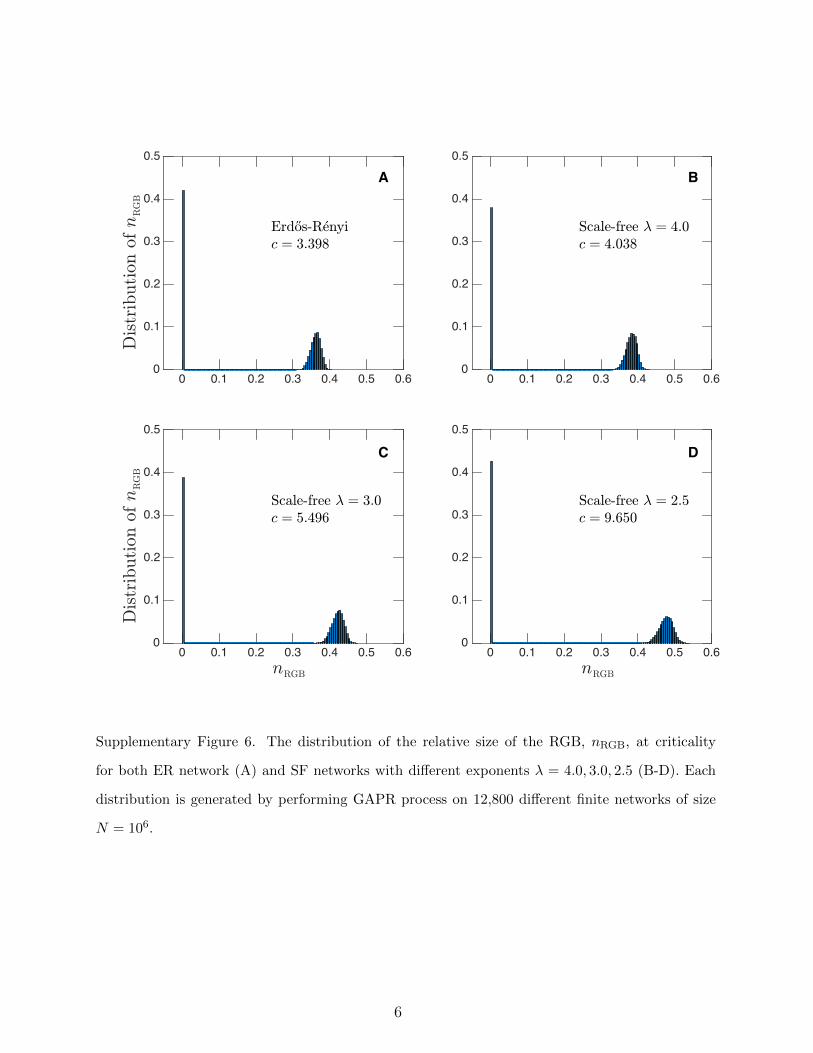
Supplementary Figure 6. The distribution of the relative size of the RGB, nRGB, at criticality

for both ER network (A) and SF networks with different exponents λ = 4.0, 3.0, 2.5 (B-D). Each

distribution is generated by performing GAPR process on 12,800 different finite networks of size

N = 106.

6

= = =

= +

+ + = 1

A

B

C

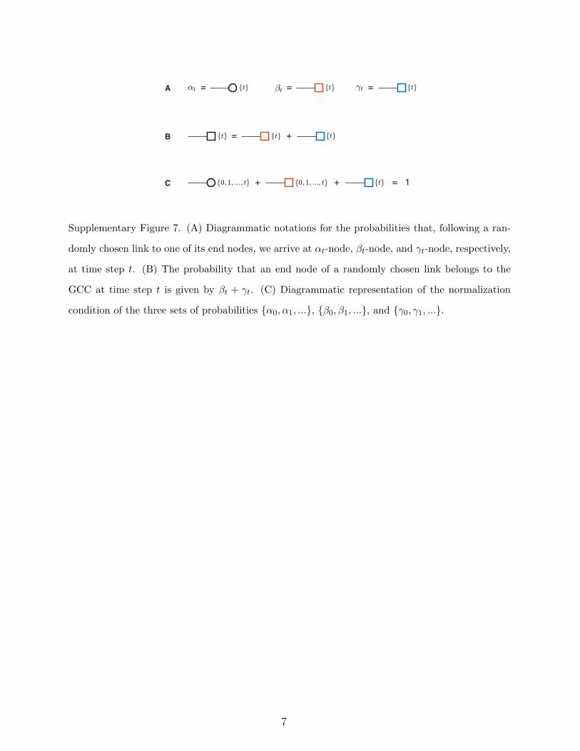
Supplementary Figure 7. (A) Diagrammatic notations for the probabilities that, following a ran-

domly chosen link to one of its end nodes, we arrive at αt-node, βt-node, and γt-node, respectively,

at time step t. (B) The probability that an end node of a randomly chosen link belongs to the

GCC at time step t is given by βt + γt. (C) Diagrammatic representation of the normalization

condition of the three sets of probabilities {α0, α1, ...}, {β0, β1, ...}, and {γ0, γ1, ...}.

7

= + + + ...+

= + + + ...

Supplementary Figure 8. Diagrammatic representations of the self-consistent equations for α0 and

β0.

8

= +...+ ...+...

...

}

}

+

+ + +...+...

...

}

}

...+

= ++ +...

} ......

}... } ...+

Supplementary Figure 9. Diagrammatic representations of the self-consistent equations for αt and

βt.

9

= ++ +... ...+

} ...

}

...

in a FCC

= ++ +...

} ...

...

}

... }...+

in the GCC

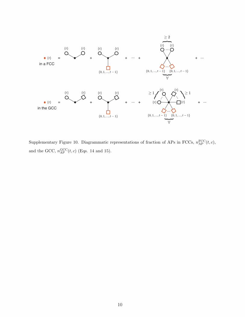
Supplementary Figure 10. Diagrammatic representations of fraction of APs in FCCs, nFCCAP (t, c),

and the GCC, nGCCAP (t, c) (Eqs. 14 and 15).

10

= +in the GCC

} ...

}

...

} ...

...

}

+

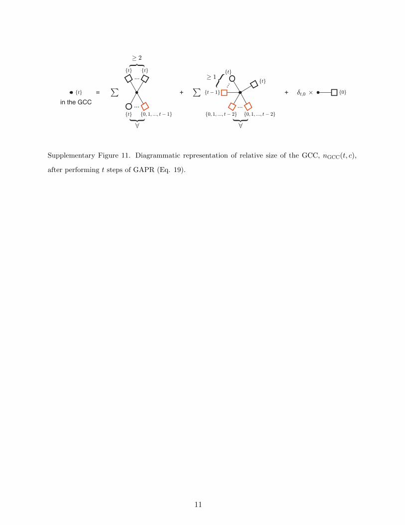
Supplementary Figure 11. Diagrammatic representation of relative size of the GCC, nGCC(t, c),

after performing t steps of GAPR (Eq. 19).

11

= ++ +... ...+in the RGB

} ...

}

...

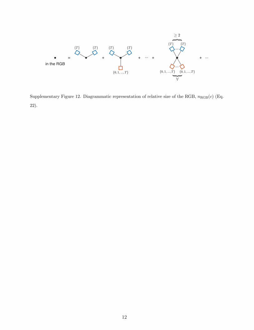
Supplementary Figure 12. Diagrammatic representation of relative size of the RGB, nRGB(c) (Eq.

22).

12

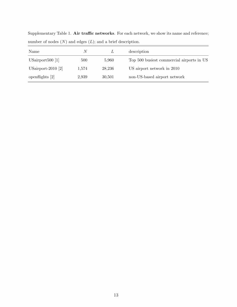
Supplementary Table 1. Air traffic networks. For each network, we show its name and reference;

number of nodes (N) and edges (L); and a brief description.

Name N L description

USairport500 [1] 500 5,960 Top 500 busiest commercial airports in US

USairport-2010 [2] 1,574 28,236 US airport network in 2010

openflights [2] 2,939 30,501 non-US-based airport network

13

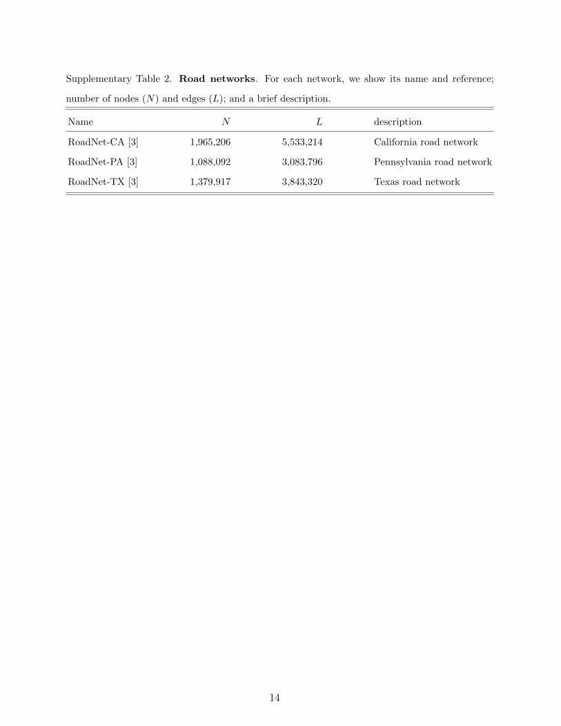
Supplementary Table 2. Road networks. For each network, we show its name and reference;



RoadNet-CA [3] 1,965,206 5,533,214 California road network

RoadNet-PA [3] 1,088,092 3,083,796 Pennsylvania road network

RoadNet-TX [3] 1,379,917 3,843,320 Texas road network

14

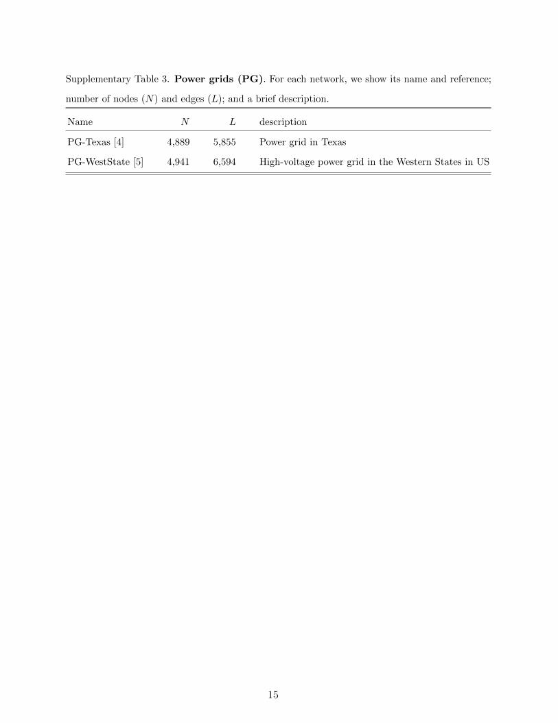
Supplementary Table 3. Power grids (PG). For each network, we show its name and reference;



PG-Texas [4] 4,889 5,855 Power grid in Texas

PG-WestState [5] 4,941 6,594 High-voltage power grid in the Western States in US

15

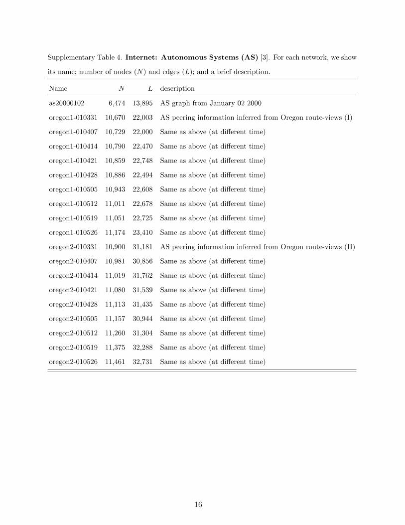
Supplementary Table 4. Internet: Autonomous Systems (AS) [3]. For each network, we show

its name; number of nodes (N) and edges (L); and a brief description.


as20000102 6,474 13,895 AS graph from January 02 2000

oregon1-010331 10,670 22,003 AS peering information inferred from Oregon route-views (I)

oregon1-010407 10,729 22,000 Same as above (at different time)








oregon2-010331 10,900 31,181 AS peering information inferred from Oregon route-views (II)









16

Supplementary Table 5. Internet: peer-to-peer (p2p) file sharing networks [3]. For each

network, we show its name; number of nodes (N) and edges (L); and a brief description.


p2p-Gnutella04 10,876 39,994 Gnutella p2p file sharing network

p2p-Gnutella05 8,846 31,839 Same as above (at different time)








17

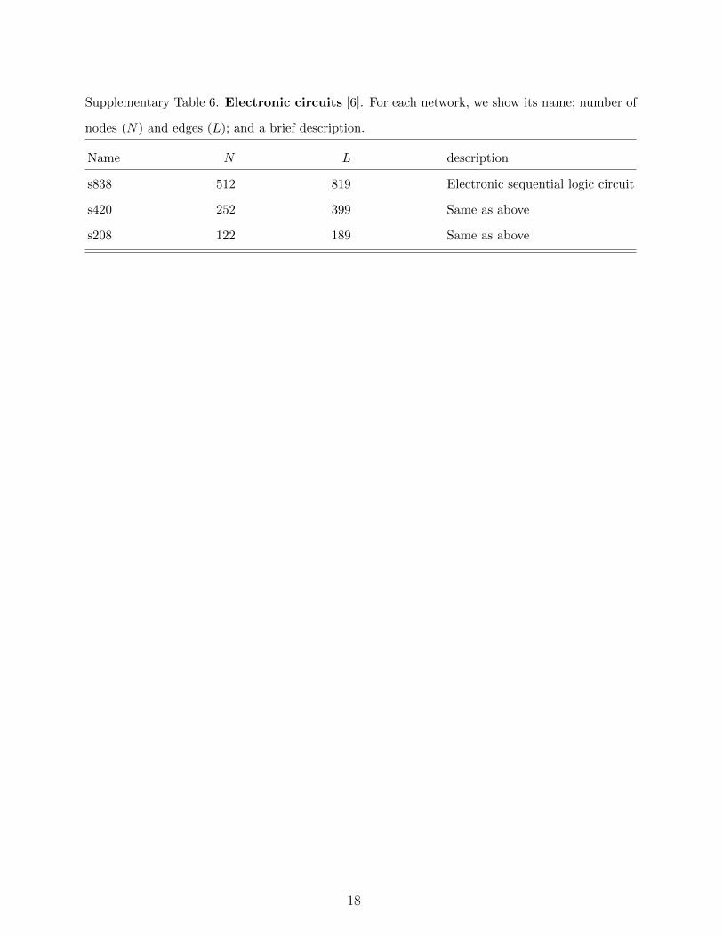
Supplementary Table 6. Electronic circuits [6]. For each network, we show its name; number of

nodes (N) and edges (L); and a brief description.


s838 512 819 Electronic sequential logic circuit

s420 252 399 Same as above

s208 122 189 Same as above

18

Supplementary Table 7. World Wide Web (WWW). For each network, we show its name and

reference; number of nodes (N) and edges (L); and a brief description.


stanford.edu [3] 281,903 1,992,636 WWW from nd.edu domain

nd.edu [7] 325,729 1,090,108 WWW from stanford.edu domain

19

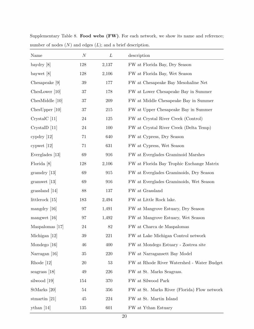
Supplementary Table 8. Food webs (FW). For each network, we show its name and reference;



baydry [8] 128 2,137 FW at Florida Bay, Dry Season

baywet [8] 128 2,106 FW at Florida Bay, Wet Season

Chesapeake [9] 39 177 FW at Chesapeake Bay Mesohaline Net

ChesLower [10] 37 178 FW at Lower Chesapeake Bay in Summer

ChesMiddle [10] 37 209 FW at Middle Chesapeake Bay in Summer

ChesUpper [10] 37 215 FW at Upper Chesapeake Bay in Summer

CrystalC [11] 24 125 FW at Crystal River Creek (Control)

CrystalD [11] 24 100 FW at Crystal River Creek (Delta Temp)

cypdry [12] 71 640 FW at Cypress, Dry Season

cypwet [12] 71 631 FW at Cypress, Wet Season

Everglades [13] 69 916 FW at Everglades Graminoid Marshes

Florida [8] 128 2,106 FW at Florida Bay Trophic Exchange Matrix

gramdry [13] 69 915 FW at Everglades Graminoids, Dry Season

gramwet [13] 69 916 FW at Everglades Graminoids, Wet Season

grassland [14] 88 137 FW at Grassland

littlerock [15] 183 2,494 FW at Little Rock lake.

mangdry [16] 97 1,491 FW at Mangrove Estuary, Dry Season

mangwet [16] 97 1,492 FW at Mangrove Estuary, Wet Season

Maspalomas [17] 24 82 FW at Charca de Maspalomas

Michigan [12] 39 221 FW at Lake Michigan Control network

Mondego [16] 46 400 FW at Mondego Estuary - Zostrea site

Narragan [16] 35 220 FW at Narragansett Bay Model

Rhode [12] 20 53 FW at Rhode River Watershed - Water Budget

seagrass [18] 49 226 FW at St. Marks Seagrass.

silwood [19] 154 370 FW at Silwood Park

StMarks [20] 54 356 FW at St. Marks River (Florida) Flow network

stmartin [21] 45 224 FW at St. Martin Island

ythan [14] 135 601 FW at Ythan Estuary

20

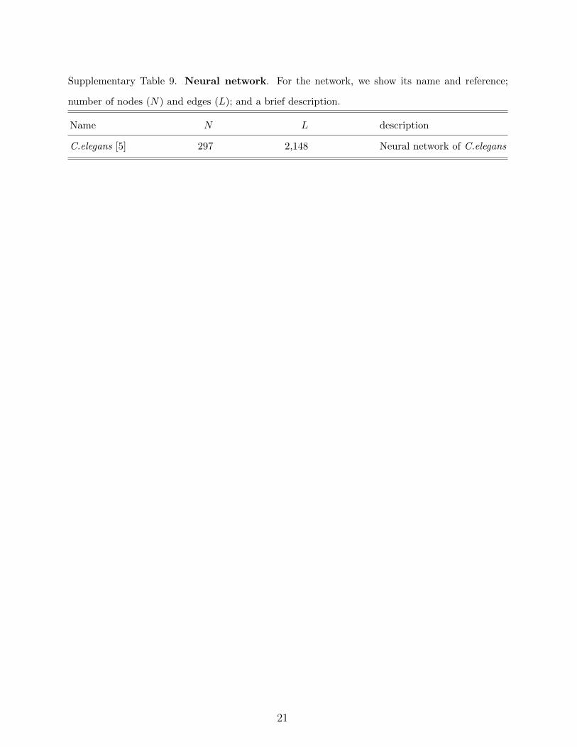
Supplementary Table 9. Neural network. For the network, we show its name and reference;



C.elegans [5] 297 2,148 Neural network of C.elegans

21

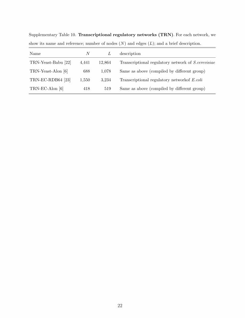
Supplementary Table 10. Transcriptional regulatory networks (TRN). For each network, we

show its name and reference; number of nodes (N) and edges (L); and a brief description.


TRN-Yeast-Babu [22] 4,441 12,864 Transcriptional regulatory network of S.cerevisiae

TRN-Yeast-Alon [6] 688 1,078 Same as above (compiled by different group)

TRN-EC-RDB64 [23] 1,550 3,234 Transcriptional regulatory networkof E.coli

TRN-EC-Alon [6] 418 519 Same as above (compiled by different group)

22

Supplementary Table 11. Protein-protein interaction (PPI) networks of different organ-

isms [24]. For each network, we show its name; and number of nodes (N) and edges (L).

Name N L

Arabidopsis thaliana (Columbia) 8,149 26,578

Bos taurus 394 405

Caenorhabditis elegans 3,941 8,641

Candida albicans (SC5314) 370 412

Danio rerio 235 281

Drosophila melanogaster 8,212 47,730

Emericella nidulans (FGSC A4) 64 71

Escherichia coli (K12/MG1655) 136 127

Gallus gallus 336 409

Hepatitus C Virus 112 164

Homo sapiens 18,632 224,270

Human Herpesvirus 1 139 183




Human Immunodeficiency Virus 1 1,028 1,786

Mus musculus 8,512 22,623

Oryctolagus cuniculus 182 198

Plasmodium falciparum (3D7) 1,227 2,545

Rattus norvegicus 3,313 5,357

Saccharomyces cerevisiae (S288c) 6,481 333,833

Schizosaccharomyces pombe (972h) 3,963 67,796

Solanum lycopersicum 25 86

Sus scrofa 87 75

Xenopus laevis 479 683

23

Supplementary Table 12. Communication networks. For each network, we show its name and

reference; number of nodes (N) and edges (L); and a brief description.


Cellphone [25] 36,595 91,826 Call network of cell phone users

Email-Enron [3] 36,692 367,662 Email communication network from Enron

Email-EuAll [3] 265,214 420,045 Email network from a large European research institute

Email-epoch [26] 3,188 39,256 Email network in a university

UCIonline [27] 1,899 20,296 Online message network of students at UC, Irvine

WikiTalk [3] 2,394,385 5,021,410 Wikipedia talk network

24

Supplementary Table 13. Social networks. For each network, we show its name and reference;



Epinions [28] 75,888 508,837 Who-trusts-whom network of Epinions.com

college student [29, 30] 32 96 Social networks of positive sentiment (college students)

prison inmate [29, 30] 67 182 Same as above (prison inmates)

Slashdot-1 [3] 77,357 516,575 Slashdot social network

Slashdot-2 [3] 81,871 545,671 Same as above (at different time)




Twitter [3] 81,306 2,420,766 Social circles from Twitter

WikiVote [3] 7,115 103,689 Wikipedia who-votes-on-whom network

Youtube [3] 1,134,890 2,987,624 Youtube online social network

25

Supplementary Table 14. Intra-organizational networks. For each network, we show its name

and reference; number of nodes (N) and edges (L); and a brief description.


Freemans-1 [31] 34 695 Social network of network researchers

Freemans-2 [31] 34 830 Same as above (at different time)

Freemans-3 [31] 32 460 Same as above (at different time)

Consulting-1 [32] 46 879 Social network from a consulting company

Consulting-2 [32] 46 858 Same as above (different evaluation)

Manufacturing-1 [32] 77 2,326 Social network from a manufacturing company

Manufacturing-2 [32] 77 2,228 Same as above (different evaluation)

26

Supplementary Note 1 - Articulation-point-targeted attack (APTA)

A common measure of the structural integrity of a network is the size of its giant connected

component (GCC). Articulation points (APs) are natural targets if we aim for immediate

damage to the GCC. To quickly destruct the GCC, we can target the most destructive

AP whose removal will cause the most nodes disconnected from the GCC. This leads to a

brute-force strategy of network destruction:

Step-1: Identify all the APs in the current network, which can be achieved by a linear-time

algorithm based on depth-first search [33].

Step-2: For each AP, calculate its “destructivity”, i.e. how many nodes will be disconnected

from the GCC after its removal.

Step-3: Rank all the APs based on their destructivities, and remove the most destructive

one together with the links attaching to it. (In case the most destructive APs are not

unique, randomly choose one of them to remove.)

Step-4: Repeat steps 1-3 until the network is totally destroyed or left with a residual giant

biconnected component (RGB), in which no APs exist.

Hereafter we call this iterative process AP-targeted attack.

To demonstrate the efficiency of APTA in reducing the size of the GCC, we compare

it with two other network destruction strategies based on the following node centrality

measures:

• Degree. In this strategy, we iteratively remove the node with the highest degree in

the current network [34, 35]. (In case the highest-degree nodes are not unique, we

randomly choose one of them to remove.) Degrees of the remaining nodes will be

recalculated after each node removal.

• Collective influence. The collective influence (CI) of node i is defined as the product

of its reduced degree (ki − 1) and the total reduced degree of all nodes at distance

l from it, i.e. CIl(i) = (ki − 1)∑

j∈∂Ball(i,l)(kj − 1), where ∂Ball(i, l) is the frontier

of a ball of radius l centered at node i (i.e. the set of the l-th nearest neighbors of

node i) [36]. In each step, we compute the CI of every node, and remove the node

27

with the largest CI. (In case the highest-CI nodes are not unique, we randomly choose

one of them to remove.) It has been shown that, in locally tree-like large networks,

the CI-based attack gives the optimal threshold, i.e. the minimal fraction of removed

nodes that totally destroys the GCC [36]. Note that, for l = 0, this method is reduced

to the degree-based network destruction.

We compute the relative size of the GCC, denoted as nGCC, as a function of the frac-

tion of removed nodes q by using the three above-mentioned network destruction strategies

in two classical configuration models (Supplementary Fig. 1A) and five different types of

real-world networks (including technological, infrastructure, biological, communication, and

online social networks) (Supplementary Figs. 1B-F). Interestingly, we find that, given a lim-

ited “budget” (i.e. a small fraction of nodes to be removed), APTA is the most efficient

strategy in reducing GCC for both model and real networks (Supplementary Fig. 1). It

turns out that even though AP removal maximizes only the local damage to the network

in every step, and does not aim for a systemic or global breakdown of the network, for a

certain range of q this is highly efficient in damaging the entire system. Moreover, in some of

the networks, such as the road network (Supplementary Fig. 1B-2), the power grid (Supple-

mentary Fig. 1B-3), and the World Wide Web (WWW) (Supplementary Fig. 1C-1), APTA

is optimal even in the whole range of q. The reason that for those networks APTA leads

to smaller critical q than the state-of-the-art CI-based method is because these networks

are either spatially embedded or/and rich in loops, in which the CI-based method is not

guaranteed to be efficient.

Note that, even for networks with rather big RGBs (Supplementary Figs. 1A-2, A-4,

F-3), ATPA is still very efficient till the GCC becomes biconnected (or becomes an RGB),

where the process of APTA terminates.

28

Supplementary Note 2 - Residual giant biconnected component

The RGB can also be obtained by the process of greedy APs removal (GAPR). Performing

GAPR on a given network consists of the following steps:

Step-1: Identify all the APs in the current network by the depth-first search algorithm [33].

Step-2: Simultaneously remove all the APs and the links attaching to them in the current

network.

Step-3: Repeat steps 1-2 until no APs exist in the network.

For a general network of finite size, GAPR and APTA do not necessarily yield exactly the

same RGB. In fact, the RGB obtained from the former is unique (because the GAPR process

is deterministic), while the RGB obtained from the latter could be history-dependent (there

may be multiple most destructive APs in each step).

For a given network, we denote the sets of nodes in the two RGBs associated with the

two processes as VGAPR and VAPTA, respectively. The overlap between the two RGBs can be

measured by the classical Jaccard index:

overlap =|VGAPR

⋂VAPTA|

|VGAPR

⋃VAPTA|

. (1)

In Supplementary Fig. 2, we show the relative sizes of the two RGBs, as well as the

overlap between them. We find that the two RGBs significantly overlap for both model

networks and real-world networks.

29

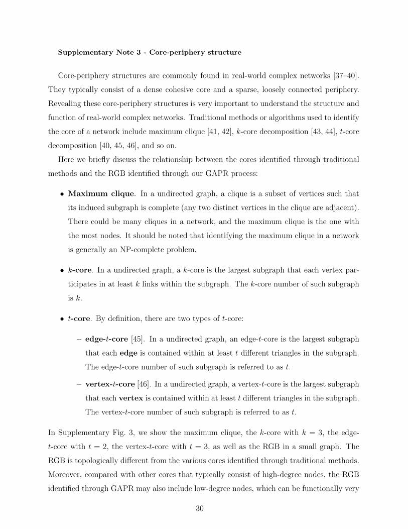
Supplementary Note 3 - Core-periphery structure

Core-periphery structures are commonly found in real-world complex networks [37–40].

They typically consist of a dense cohesive core and a sparse, loosely connected periphery.

Revealing these core-periphery structures is very important to understand the structure and

function of real-world complex networks. Traditional methods or algorithms used to identify

the core of a network include maximum clique [41, 42], k-core decomposition [43, 44], t-core

decomposition [40, 45, 46], and so on.

Here we briefly discuss the relationship between the cores identified through traditional

methods and the RGB identified through our GAPR process:

• Maximum clique. In a undirected graph, a clique is a subset of vertices such that

its induced subgraph is complete (any two distinct vertices in the clique are adjacent).

There could be many cliques in a network, and the maximum clique is the one with

the most nodes. It should be noted that identifying the maximum clique in a network

is generally an NP-complete problem.

• k-core. In a undirected graph, a k-core is the largest subgraph that each vertex par-

ticipates in at least k links within the subgraph. The k-core number of such subgraph

is k.

• t-core. By definition, there are two types of t-core:

– edge-t-core [45]. In a undirected graph, an edge-t-core is the largest subgraph

that each edge is contained within at least t different triangles in the subgraph.

The edge-t-core number of such subgraph is referred to as t.

– vertex-t-core [46]. In a undirected graph, a vertex-t-core is the largest subgraph

that each vertex is contained within at least t different triangles in the subgraph.

The vertex-t-core number of such subgraph is referred to as t.

In Supplementary Fig. 3, we show the maximum clique, the k-core with k = 3, the edge-

t-core with t = 2, the vertex-t-core with t = 3, as well as the RGB in a small graph. The

RGB is topologically different from the various cores identified through traditional methods.

Moreover, compared with other cores that typically consist of high-degree nodes, the RGB

identified through GAPR may also include low-degree nodes, which can be functionally very

30

important but always ignored in traditional methods. Hence, our AP-based decomposition

method provides us a new angle to analyze and understand the organization of real-world

complex networks.

31

Supplementary Note 4 - Theoretical Framework

A. Local tree approximation

Local tree approximation assumes that in the thermodynamics limit (i.e. the network

size N → ∞) there are no finite loops in the network and only infinite loops exist. This

approximation directly leads to three important network properties [35, 47–50]:

1. All of the finite connected components (FCCs) are trees. Loops (of infinite length)

only exist in the GCC;

2. There can be only one GCC in the network [49];

3. For any node in the network, its neighbors become disconnected or independent from

each other if the node and its attaching links are removed.

In our theoretical framework, we use the above local tree approximation to study the

GAPR process in large uncorrelated random networks with arbitrary degree distribution

P (k) and finite mean degree c =∑

k kP (k). Note that the local tree approximation becomes

exact for networks with finite second moment of the degree distribution, such as Erdos-Renyi

(ER) networks or scale-free (SF) networks with degree exponent λ > 3. However, we can

still use this approximation to study networks with diverging second moment of the degree

distribution, such as SF networks with λ ≤ 3. It has been demonstrated in literature that

the local tree approximation obtains very accurate results for various network problems [49].

Actually, this approximation has been widely used in studying loopy networks [49, 51]. Here

we find that it works very well for studying AP-related problems in SF networks with λ ≤ 3

(see Supplementary Note 6 for numerical simulations).

B. Discrete-time dynamics of GAPR

The deterministic GAPR process is naturally associated with a temporal order. At t = 0,

we have the original network. At t = T , i.e. the last time step of GAPR, no AP exists in

the network, and the GAPR process terminates. At each time step t, we denote the fraction

of APs and the relative size of the GCC as nAP(c, t) and nGCC(c, t), respectively, where c is

32

the mean degree of the original network. The RGB is nothing but the GCC at the last time

step, whose relative size is denoted as nRGB(c) = nGCC(c, T ).

At each time step t during the GAPR process in a network G, we classify the remaining

nodes into the following three categories or states:

1. αt-nodes: nodes that belong to FCCs at time t (note that by definition αt-nodes

include APs in FCCs);

2. βt-nodes: nodes that are APs in the GCC at time t;

3. γt-nodes: nodes that are not APs and belong to the GCC at time t. Note that if a

node is a γt-node at time t, this node must be γτ -node with τ < t.

Note that the notations βt and γt here have totally different meanings from the critical

exponents mentioned in the main text.

According to the local tree approximation, the state of a randomly chosen node i can be

determined by the states of its neighbors in G\i, i.e. the induced subgraph of G with node i

and all its links removed. In order words, in order to determine the state of a node, we need

to know the states of its neighbors. Therefore, at each time step t, we need to know the

probability that, following a randomly chosen link to one of its end nodes, this node belongs

to any of the above categories after this link is removed. These probabilities are denoted as

αt, βt, and γt, respectively. Note that for convenience sake here we use the same notation to

denote both the state of a node and the probability of a node in that state. To be precise,

hereafter when we consider the state of a neighbor of a given node i, we mean the state of

the neighbor in the induced subgraph G\i. Also, when we mention the state of an end node

of a chosen link l, we mean the state of the node in G\l, i.e. the induced subgraph of G with

link l removed. According to the definitions of βt and γt, the probability that an end node

of a randomly chosen link belongs to the GCC at time step t is just βt + γt.

The GAPR process can be fully characterized by the three sets of probabilities {α0, α1, ...},

{β0, β1, ...}, and {γ0, γ1, ...}. Note that every node must belong to one of the three categories,

which means the three sets of probabilities are not independent from each other. Specifically,

at time step t, the probability γt can be derived by the other two sets of probabilities through

the following normalization condition:

t∑τ=0

ατ +t∑

τ=0

βτ + γt = 1. (2)

33

Supplementary Figure 7 shows the diagrammatic representations of these probabilities; the

probability that an end node of a randomly chosen link belongs to the GCC at time step t;

and the normalization equation 2.

Thanks to Eq. 2, hereafter all the equations will be written in terms of αt and βt only.

We can calculate {α0, α1, ...} and {β0, β1, ...} in an iterative way. At first, we consider the

initial time step t = 0. The self-consistent equations for α0 and β0 are given by

α0 =∞∑k=1

Q(k) (α0)k−1 (3)

β0 =∞∑k=3

Q(k)[1− (1− α0)

k−1 − (α0)k−1], (4)

where

Q(k) = kP (k)/c (5)

is the degree distribution of the nodes that we arrive at by following a randomly chosen link

(a.k.a. the excess degree distribution) [52, 53]. We derive the above equations based on the

following observations:

• α0-node: its neighbors can only be α0-nodes;

• β0-node: since it is an AP node, at least one of its neighbors is an α0-node. Moreover,

since it belongs to the GCC, at lease one of its neighbors is not an α0-node.

Note that, due to the local tree approximation, removal of an AP in the GCC can only cause

a finite number of nodes disconnected from the GCC, and there exists no such an AP that

its removal breaks down the GCC into two infinitely large components. The diagrammatic

representations of Eqs. 3 and 4 are shown in Supplementary Fig. 8.

For the t-th GAPR time step (t > 0), we can compute αt and βt as follows:

αt =∞∑k=1

Q(k)

(αt +

t−1∑τ=0

βτ

)k−1

−∞∑k=1

Q(k)

(t−2∑τ=0

βτ

)k−1

(6)

βt =∞∑k=3

Q(k)k−2∑s=1

(k − 1

s

)(1−

t∑τ=0

ατ −t−1∑τ=0

βτ

)s

×k−1−s∑r=1

(k − 1− s

r

)(αt)

r

(t−1∑τ=0

βτ

)k−1−s−r

. (7)

The derivations of Eqs. 6 and 7 are based on the following observations:

34

• αt-node: First of all, its neighbors can only be αt-nodes or βτ -nodes with τ < t

(because if one of its neighbors is ατ -node with τ < t, this node will be an AP before

time step t and hence would have already been removed; if one of its neighbor is βt-

node, this node will belong to the GCC at time step t). Second, its neighbors can not

be simultaneously all βτ -nodes with τ < t− 1. Otherwise this node will be a leaf node

before time step t− 1, and will become an isolated node before the t-th time step. In

this case, we can not reach this node through a randomly chosen link at time step t.

• βt-node: First of all, its neighbors can not be ατ -nodes with τ < t, otherwise this node

would have been removed before time step t. Second, since it is an AP node, at least

one of its neighbors is an αt-node. Finally, since this node belongs to the GCC, at

least one of its neighbors is neither αt-node nor βτ -node with τ < t.

The diagrammatic representations of Eqs. 6 and 7 are shown in Supplementary Fig. 9.

Combining Eqs. 3, 4, 6, and 7, we obtain a complete set of discrete-time dynamic

equations for the GAPR process:

α0 = G1(α0) (8)

αt>0 = G1

(αt +

t−1∑τ=0

βτ

)−G1

(t−2∑τ=0

βτ

)(9)

βt = G1

(1−

t−1∑τ=0

ατ

)−G1

(1−

t∑τ=0

ατ

)−G1

(αt +

t−1∑τ=0

βτ

)+G1

(t−1∑τ=0

βτ

), (10)

where

G1(x) =∑k

Q(k)xk−1 (11)

is the generating function of the branching processes [48].

By solving the above self-consistent equations, we obtain {α0, α1, ...} and {β0, β1, ...},

which govern the whole process of GAPR. With these two sets of probabilities, we can

compute any quantities of interest, such as the total number of GAPR steps, the fraction of

APs, the relative size of the GCC and the RGB, and so on.

C. Total number of GAPR steps

It should be noted from Eqs. 8, 9, and 10 that αt and βt depend not only on the previous

time step t − 1, but also on the entire history of GAPR, from the 0-th to the (t − 1)-th

35

time steps. Hence to calculate T , the total number of GAPR steps, we have to solve the

equations from the initial step to the T -th step when the GAPR process stops. Since the

GAPR process terminates when there is no APs left in the network, T can be determined

by requiring

αT = 0 (12)

βT = 0. (13)

Note that, according to Eq. 9, βT−1 is also zero, otherwise αT will have a non-zero solution.

D. Fraction of articulation points

Consider the fraction of APs at time step t during the GAPR process, nAP(t, c), which

also represents the probability that a randomly chosen node is an AP at t-th step. We can

calculate nAP(t, c) as the sum of the following two parts:

1. nGCCAP (t, c): fraction of APs that belong to the GCC whose removal splits the GCC

into a smaller GCC and many FCCs;

2. nFCCAP (t, c): fraction of APs that belong to FCCs whose removal splits FCCs into smaller

FCCs.

With similar theoretical considerations as deriving equations for αt and βt, we have

nFCCAP (t, c) =

∞∑k=2

P (k)k∑s=2

(k

s

)(αt)

s

(t−1∑τ=0

βτ

)k−s

(14)

nGCCAP (t, c) =

∞∑k=2

P (k)k−1∑s=1

(k

s

)(1−

t∑τ=0

ατ −t−1∑τ=0

βτ

)s

×k−s∑r=1

(k − sr

)( t∑τ=0

ατ

)r( t−1∑τ=0

βτ

)k−s−r

. (15)

These two equations can be understood as follows:

• AP in FCCs, nFCCAP (t, c): First of all, since the node belongs to an FCC, its neighbor

can only be αt-nodes or βτ -nodes with τ < t. Second, since the node is an AP, at least

two of its neighbors are αt-nodes. Otherwise, it would be a leaf node or an isolated

node at time step t.

36

• AP in the GCC, nGCCAP (t, c): First of all, its neighbors can not be ατ -nodes with τ < t,

otherwise this node would have already been removed before time step t. Second, since

it is an AP node, at least one of its neighbors is an αt-node. Finally, since this node

belongs to the GCC, at least one of its neighbors is neither αt-node nor βτ -node with

τ < t.

The diagrammatic representations of Eqs. 14 and 15 are shown in Supplementary Fig. 10.

Combing Eqs. 14 and 15, we obtain the fraction of APs at time step t as

nAP(t, c) = nFCCAP (t, c)+nGCC

AP (t, c) = G0

(1−

t−1∑τ=0

ατ

)−G0

(1−

t∑τ=0

ατ

)−cαtG1

(t−1∑τ=0

βτ

),

(16)

where

G0(x) =∑k

P (k)xk (17)

is the generating function of the degree distribution P (k).

The fraction of APs in the original network, nAP(c), can be obtained by substituting

t = 0 into Eq. 16, yielding

nAP(c) = nAP(0, c) = 1−G0 (1− α0)− cα0G1 (0) . (18)

E. The giant connected component

Another quantity of interest is the relative size of the GCC, nGCC(t, c), after performing

a given t steps of GAPR in a network. We can compute nGCC(t, c) as follows:

nGCC(t) =∞∑k=2

P (k)k∑s=2

(k

s

)(αt +

t−1∑τ=0

βτ

)k−s(1−

t∑τ=0

ατ −t−1∑τ=0

βτ

)s

+∞∑k=2

P (k)

(k

1

)(1−

t∑τ=0

ατ −t−1∑τ=0

βτ

)k−1∑r=1

(k − 1

r

)(αt + βt−1)

r

(t−2∑τ=0

βτ

)k−1−r

+δt,0P (1) (1− α0) , (19)

where the Kronecker delta function δjk = 1 if j = k, and 0 otherwise. This equation can be

understood as follows:

• For any node in the GCC at time step t, at least one of its neighbors belongs to the

GCC at current time step. Moreover, none of its neighbors is ατ -nodes with τ < t,

otherwise this node would have already been removed as an AP before time step t.

37

• The first term on the right hand side of Eq. 19 accounts for the nodes with at least

two neighbors belonging to the GCC.

• The second term accounts for the nodes with only one neighbor in the GCC. It should

be noted that, for each of these nodes, at least one of its neighbors is αt-nodes or

βt−1-nodes. Otherwise, this node would be a leaf node before time step t, and thus

will become an isolated node at time step t.

• We only consider nodes with degree larger than 2 in the first two terms. This is

because any leaf nodes will become isolated ones right after the first step of GAPR. If

we include the ordinary percolation as the 0-th time step in our GAPR process, leaf

nodes can also belong to the GCC at the 0-th step, which is the third term.

The diagrammatic representation of Eq. 19 is shown in Supplementary Fig. 11. After some

algebra, we can rewrite nGGC(t, c) in terms of generating functions:

nGGC(t, c) = G0

(1−

t−1∑τ=0

ατ

)−G0

(αt +

t−1∑τ=0

βτ

)−(1− δτ,0) c

(1−

t∑τ=0

ατ −t−1∑τ=0

βτ

)G1

(t−2∑τ=0

βτ

),

(20)

which eases later calculations. Note that the relative size of the GCC for ordinary percolation

can be recovered by substituting t = 0 into the above equation, yielding

nGCC(0) = 1−G0 (α0) . (21)

F. The residual giant biconnected component

If we keep performing GAPR in a network until there is no AP left, depending on the

initial structure of the network, it could be totally destructed or left with an RGB. The

relative size of the RGB can be calculated as

nRGB(c) =∞∑k=2

P (k)k∑s=2

(k

s

)(1−

T∑τ=0

ατ −T∑τ=0

βτ

)T∑τ=0

βτ , (22)

which is based on the following observations:

• For any node in the RGB, its neighbors can not be αt-nodes at any t. Otherwise, this

node is removable as an AP.

38

• Since the RGB is biconnected, each of its nodes must be connected to at least two

other RGB nodes. The probability that an end node of a randomly chosen link belongs

to the RGB is 1−∑T

τ=0 ατ −∑T

τ=0 βτ .

The diagrammatic representation of Eq. 22 is shown in Supplementary Fig. 12. After some

algebra, Eq. 22 can be rewritten in terms of generating functions as:

nRGB(c) = G0

(1−

T∑τ=0

ατ

)−G0

(T∑τ=0

βτ

)− c

(1−

T∑τ=0

ατ −T∑τ=0

βτ

)G1

(T∑τ=0

βτ

). (23)

Note that the RGB is nothing but the GCC at the last time step T , we can also obtain

the above equation by substituting t = T and also αT = 0, βT = 0, βT−1 = 0 into the Eq.

20 of nGCC(t, c).

G. Canonical model networks

The developed theoretical framework works for complex networks with any prescribed

degree distribution. In this work, we consider two canonical model networks: ER networks

and SF networks, which have specific degree distributions.

1. Erdos-Renyi network

For ER random network, the degree distribution P (k) in the thermodynamic limit follows

the Poisson distribution, i.e.

P (k) =e−cck

k!, (24)

where c =∑∞

k=0 kP (k) is the mean degree. The generating functions are given by

G0(x) = G1(x) = ec(x−1). (25)

Substituting the above equation into Eqs. 8, 9, and 10, we obtain the dynamic equations

of the GAPR process on ER network:

α0 = exp [c (α0 − 1)] (26)

αt>0 = exp

[c

(αt +

t−1∑τ=0

βτ − 1

)]− exp

[c

(t−2∑τ=0

βτ − 1

)](27)

39

βt = exp

(−c

t−1∑τ=0

ατ

)−exp

(−c

t∑τ=0

ατ

)−exp

[c

(αt +

t−1∑τ=0

βτ − 1

)]+exp

[c

(t−1∑τ=0

βτ − 1

)].

(28)

Similarly, the fraction of APs is given by

nAP(t, c) = exp

(−c

t−1∑τ=0

ατ

)− exp

(−c

t∑τ=0

ατ

)− cαt exp

[c

(t−1∑τ=0

βτ − 1

)]. (29)

Hence the fraction of APs in the original network at t = 0 is given by

nAP(c) = nAP(0, c) = 1− exp (−cα0)− cα0 exp (−c) . (30)

The relative size of the GCC at the t-th time step is given by

nGCC(t) =exp

(−c

t−1∑τ=0

ατ

)− exp

[c

(αt +

t−1∑τ=0

βτ − 1

)]

− (1− δτ,0) c

(1−

t∑τ=0

ατ −t−1∑τ=0

βτ

)exp

[c

(t−2∑τ=0

βτ − 1

)]. (31)

The relative size of the RGB is

nRGB(c) = exp

(−c

T∑τ=0

ατ

)−exp

[c

(T∑τ=0

βτ − 1

)]−c

(1−

T∑τ=0

ατ −T∑τ=0

βτ

)exp

[c

(T∑τ=0

βτ − 1

)].

(32)

2. Scale-free network

We use the static model to generate asymptotically SF networks with tunable network

size N , mean degree c, and degree distribution exponent λ > 2 [54].

This model can be described as follows:

Step-1: We start with N isolated nodes, which are labeled from 1 to N . Each node is

assigned a weight pi ∼ i−a, where a = 1λ−1 .

Step-2: We independently pick up two nodes according to their assigned weights, and add

a link between these two nodes if they have not been connected before. Self-links and

double-links are forbidden.

Step-3: Repeat step-2 until M = cN/2 links have been added into the network.

40

In the thermodynamic limit, the degree distribution of the static model can be analytically

derived [55, 56]:

P (k) =[c(1− a)]k

ak!

∫ ∞1

dx exp[−c(1− a)x]xk−1−1/a. (33)

The generating function of the degree distribution P (k) is given by

G0(x) =∞∑k=0

[c(1− a)]k

ak!

∫ ∞1

dy exp[−c(1− a)y]yk−1−1/axk

=1

a

∫ ∞1

dy exp[−c(1− a)y]y−1−1/a∞∑k=0

[c(1− a)xy]k

k!

=1

a

∫ ∞1

dy exp[−c(1− a)(1− x)y]y−1−1/a, (34)

where ec(1−a)xy =∑∞

k=0[c(1−a)xy]k

k!is used in the last step. Similarly, the generation function

of the excess degree distribution Q(k) is derived as

G1(x) =G′0(x)

G′0(1)=

1− aa

∫ ∞1

dy exp[−c(1− a)(1− x)y]y−1/a. (35)

By defining

En(x) =

∫ ∞1

e−xyy−ndy, (36)

G0(x) and G1(x) can be rewritten as

G0(x) =1

aE1+ 1

a[c(1− a)(1− x)] (37)

G1(x) =1− aa

E 1a[c(1− a)(1− x)] (38)

where the fact ∂En(x)∂x

= −En−1(x) has been used.

Substituting the above equations into Eqs. 8, 9, and 10, we obtain the dynamic equations

of the GAPR process for the static model:

α0 =1− aa

E 1a

[c (1− a) (1− α0)] (39)

αt>0 =1− aa

{E 1

a

[c (1− a)

(1− αt −

t−1∑τ=0

βτ

)]− E 1

a

[c (1− a)

(1−

t−2∑τ=0

βτ

)]}(40)

βt =1− aa

{E 1

a

[c (1− a)

t−1∑τ=0

ατ

]− E 1

a

[c (1− a)

t∑τ=0

ατ

]

−E 1a

[c (1− a)

(1− αt −

t−1∑τ=0

βτ

)]− E 1

a

[c (1− a)

(1−

t−1∑τ=0

βτ

)]}. (41)

41

Similarly, the fraction of APs is given by

nAP(t, c) =1

a

{E1+ 1

a

[c (1− a)

t−1∑τ=0

ατ

]− E1+ 1

a

[c (1− a)

t∑τ=0

ατ

]}

−cαt(1− a)

aE 1

a

[c (1− a)

(1−

t−1∑τ=0

βτ

)]. (42)

Hence the fraction of APs in the original network at t = 0 is

nAP(c) = nAP(0, c) = 1− 1

aE1+ 1

a[c(1− a)α0]−

cα0(1− a)

aE 1

a[c(1− a)]. (43)

The relative size of the GCC at the t-th time step is given by

nGCC(t) =1

a

{E1+ 1

a

[c (1− a)

t−1∑τ=0

ατ

]− E1+ 1

a

[c (1− a)

(1− αt −

t−1∑τ=0

βτ

)]}

− (1− δτ,0)c(1− a)

a

(1−

t∑τ=0

ατ −t−1∑τ=0

βτ

)E 1

a

[c (1− a)

(1−

t−2∑τ=0

βτ

)].(44)

The relative size of the RGB is

nRGB(c) =1

a

{E1+ 1

a

[c (1− a)

T∑τ=0

ατ

]− E1+ 1

a

[c (1− a)

(1−

T∑τ=0

βτ

)]}

−c(1− a)

a

(1−

T∑τ=0

ατ −T∑τ=0

βτ

)E 1

a

[c (1− a)

(1−

T∑τ=0

βτ

)]. (45)

42

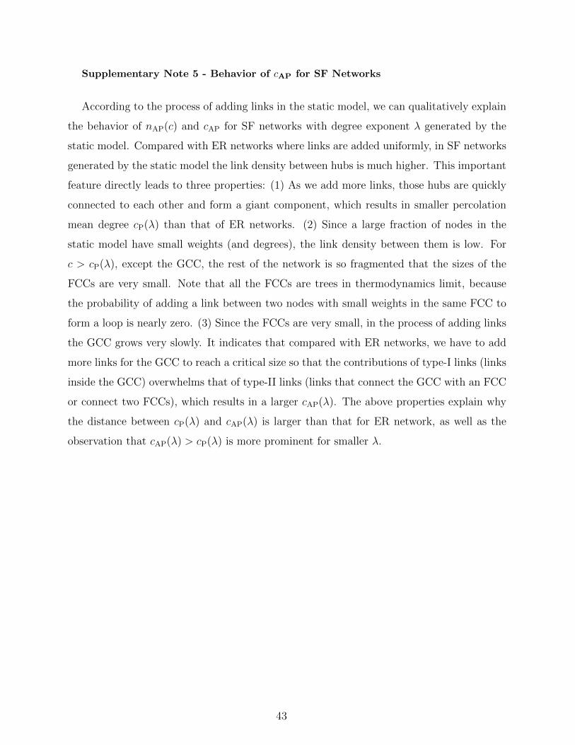
Supplementary Note 5 - Behavior of cAP for SF Networks

According to the process of adding links in the static model, we can qualitatively explain

the behavior of nAP(c) and cAP for SF networks with degree exponent λ generated by the

static model. Compared with ER networks where links are added uniformly, in SF networks

generated by the static model the link density between hubs is much higher. This important

feature directly leads to three properties: (1) As we add more links, those hubs are quickly

connected to each other and form a giant component, which results in smaller percolation

mean degree cP(λ) than that of ER networks. (2) Since a large fraction of nodes in the

static model have small weights (and degrees), the link density between them is low. For

c > cP(λ), except the GCC, the rest of the network is so fragmented that the sizes of the

FCCs are very small. Note that all the FCCs are trees in thermodynamics limit, because

the probability of adding a link between two nodes with small weights in the same FCC to

form a loop is nearly zero. (3) Since the FCCs are very small, in the process of adding links

the GCC grows very slowly. It indicates that compared with ER networks, we have to add

more links for the GCC to reach a critical size so that the contributions of type-I links (links

inside the GCC) overwhelms that of type-II links (links that connect the GCC with an FCC

or connect two FCCs), which results in a larger cAP(λ). The above properties explain why

the distance between cP(λ) and cAP(λ) is larger than that for ER network, as well as the

observation that cAP(λ) > cP(λ) is more prominent for smaller λ.

43

Supplementary Note 6 - Numerical Simulations

We have performed extensive numerical simulations to confirm our analytical results.

Supplementary Figure 4 shows the simulation results of the fraction of APs, nAP(c, t),

as a function of mean degree c at different time steps for ER networks and SF networks

(constructed from the ER model and the static model) with different degree exponents λ.

For comparison, analytical results for infinitely large networks are also shown (in lines).

The comparison between simulation results and analytical predictions of the relative size

of the GCC, nGCC(c, t), is shown in Supplementary Fig. 5. Note that, in Supplementary

Figs. 4 and 5, the deviation of the simulation results from the theoretical prediction for SF

networks with exponent λ = 2.5 owes to degree correlations in the constructed scale-free

networks, which become prominent as λ→ 2 [57].

In Supplementary Fig. 6, we show the simulation results of the distribution of the relative

size of the RGB, nRGB, at criticality for both ER network and SF networks with different

degree exponents. The bimodal distribution is another evidence that nRGB undergoes a

discontinuous jump from zero to a large finite value at the critical point [49].

44

Supplementary Note 7 - Network Datasets

All the real-world networks analyzed in this work are listed and briefly described in the

Supplementary Tables 1-14. For each network, we show its name and reference; number of

nodes (N) and edges (L); and a brief description (unless it is clear from the network type).

45

SUPPLEMENTARY REFERENCES

[1] Colizza, V., Pastor-Satorras, R. & Vespignani, A. Reaction–diffusion processes and metapop-

ulation models in heterogeneous networks. Nature Physics 3, 276–282 (2007).

[2] Opsahl, T. Why anchorage is not (that) important: Binary ties and sample selection. Avail-

able at http://toreopsahl.com/2011/08/12/why-anchorage-is-not-that-important-binary-ties-

and-sample-selection/ (2011).

[3] Leskovec, J. & Krevl, A. SNAP Datasets: Stanford Large Network Dataset Collection. Avail-

able at https://snap.stanford.edu/data/ (2014).

[4] Bianconi, G., Gulbahce, N. & Motter, A. E. Local structure of directed networks. Physical

Review Letters 100, 118701 (2008).

[5] Watts, D. J. & Strogatz, S. H. Collective dynamics of ‘small-world’ networks. Nature 393,

440–442 (1998).

[6] Milo, R. et al. Network motifs: simple building blocks of complex networks. Science 298,

824–827 (2002).

[7] Albert, R., Jeong, H. & Barabasi, A.-L. Internet: Diameter of the world-wide web. Nature

401, 130–131 (1999).

[8] Ulanowicz, R., Bondavalli, C. & Egnotovich, M. Network analysis of trophic dynamics in

south florida ecosystem, fy 97: The florida bay ecosystem. Annual Report to the United States

Geological Service Biological Resources Division Ref. No.[UMCES] CBL 98–123 (1998).

[9] Baird, D. & Ulanowicz, R. E. The seasonal dynamics of the Chesapeake Bay ecosystem.

Ecological Monographs 59, 329–364 (1989).

[10] Hagy, J. D. Eutrophication, hypoxia and trophic transfer efficiency in Chesapeake Bay (PhD

Dissertation, University of Maryland at College Park, 2002).

[11] Ulanowicz, R. E. Growth and development: ecosystems phenomenology (Springer Science &

Business Media, 2012).

[12] Pajek Food Web datasets. http://vlado.fmf.uni-lj.si/pub/networks/data/bio/foodweb/foodweb.htm.

[13] Ulanowicz, R., Bondavalli, C., Heymans, J. & Egnotovich, M. Network Analysis of Trophic

Dynamics in South Florida Ecosystem, FY 99: The Graminoid Ecosystem. Annual Report

to the United States Geological Service Biological Resources Division Ref. No.[UMCES] CBL

00-0176, Chesapeake Biological Laboratory, University of Maryland (2000).

46

[14] Dunne, J. A., Williams, R. J. & Martinez, N. D. Food-web structure and network theory: the

role of connectance and size. Proceedings of the National Academy of Sciences 99, 12917–12922

(2002).

[15] Martinez, N. D. Artifacts or attributes? Effects of resolution on the Little Rock Lake food

web. Ecological Monographs 61, 367–392 (1991).

[16] Patrıcio, J. M. How well do ecological indicators assess environmental status?: case studies

in coastal and estuarine ecosystems (PhD thesis, University of Coimbra, Coimbra, Portugal,

2005).

[17] Almunia, J., Basterretxea, G., Arıstegui, J. & Ulanowicz, R. Benthic-pelagic switching in a

coastal subtropical lagoon. Estuarine, Coastal and Shelf Science 49, 363–384 (1999).

[18] Christian, R. R. & Luczkovich, J. J. Organizing and understanding a winter’s seagrass foodweb

network through effective trophic levels. Ecological Modelling 117, 99–124 (1999).

[19] Memmott, J., Martinez, N. & Cohen, J. Predators, parasitoids and pathogens: species rich-

ness, trophic generality and body sizes in a natural food web. Journal of Animal Ecology 69,

1–15 (2000).

[20] Baird, D., Luczkovich, J. & Christian, R. R. Assessment of spatial and temporal variability

in ecosystem attributes of the St Marks National Wildlife Refuge, Apalachee Bay, Florida.

Estuarine, Coastal and Shelf Science 47, 329–349 (1998).

[21] Goldwasser, L. & Roughgarden, J. Construction and analysis of a large Caribbean food web.

Ecology 1216–1233 (1993).

[22] Balaji, S., Babu, M. M., Iyer, L. M., Luscombe, N. M. & Aravind, L. Comprehensive analysis

of combinatorial regulation using the transcriptional regulatory network of yeast. Journal of

Molecular Biology 360, 213–227 (2006).

[23] Gama-Castro, S. et al. RegulonDB (version 6.0): gene regulation model of Escherichia coli

K-12 beyond transcription, active (experimental) annotated promoters and Textpresso navi-

gation. Nucleic Acids Research 36, D120–D124 (2008).

[24] Stark, C. et al. BioGRID: a general repository for interaction datasets. Nucleic Acids Research

34, D535–D539 (2006).

[25] Song, C., Qu, Z., Blumm, N. & Barabasi, A.-L. Limits of predictability in human mobility.

Science 327, 1018–1021 (2010).

47

[26] Eckmann, J.-P., Moses, E. & Sergi, D. Entropy of dialogues creates coherent structures in

e-mail traffic. Proceedings of the National Academy of Sciences 101, 14333–14337 (2004).

[27] Opsahl, T. & Panzarasa, P. Clustering in weighted networks. Social Networks 31, 155–163

(2009).

[28] Richardson, M., Agrawal, R. & Domingos, P. Trust management for the semantic web. In

International semantic Web conference, 351–368 (Springer, 2003).

[29] Van Duijn, M. A., Zeggelink, E. P., Huisman, M., Stokman, F. N. & Wasseur, F. W. Evolution

of sociology freshmen into a friendship network. Journal of Mathematical Sociology 27, 153–

191 (2003).

[30] Milo, R. et al. Superfamilies of evolved and designed networks. Science 303, 1538–1542

(2004).

[31] Freeman, S. C. & Freeman, L. C. The networkers network: A study of the impact of a new

communications medium on sociometric structure (School of Social Sciences University of

Calif., 1979).

[32] Cross, R. L. & Parker, A. The hidden power of social networks: Understanding how work

really gets done in organizations (Harvard Business Review Press, 2004).

[33] Tarjan, R. E. & Vishkin, U. An efficient parallel biconnectivity algorithm. SIAM Journal on

Computing 14, 862–874 (1985).

[34] Albert, R., Jeong, H. & Barabasi, A.-L. Error and attack tolerance of complex networks.

Nature 406, 378–382 (2000).

[35] Cohen, R., Erez, K., Ben-Avraham, D. & Havlin, S. Resilience of the Internet to random

breakdowns. Physical Review Letters 85, 4626 (2000).

[36] Morone, F. & Makse, H. A. Influence maximization in complex networks through optimal

percolation. Nature 524, 65–68 (2015).

[37] Borgatti, S. P. & Everett, M. G. Models of core/periphery structures. Social Networks 21,

375–395 (2000).

[38] Rombach, M. P., Porter, M. A., Fowler, J. H. & Mucha, P. J. Core-periphery structure in

networks. SIAM Journal on Applied Mathematics 74, 167–190 (2014).

[39] Zhang, X., Martin, T. & Newman, M. E. Identification of core-periphery structure in networks.

Physical Review E 91, 032803 (2015).

48

[40] Verma, T., Russmann, F., Araujo, N., Nagler, J. & Herrmann, H. Emergence of core-

peripheries in networks. Nature Communications 7, 10441 (2016).

[41] Behzad, M. & Chartrand, G. Introduction to the Theory of Graphs (Allyn and Bacon, 1972).

[42] Harary, F. Graph Theory (Addison-Wesley, Reading, MA, 1969).

[43] Dorogovtsev, S. N., Goltsev, A. V. & Mendes, J. F. F. K-core organization of complex

networks. Physical Review Letters 96, 040601 (2006).

[44] Kitsak, M. et al. Identification of influential spreaders in complex networks. Nature Physics

6, 888–893 (2010).

[45] Zhang, Y. & Parthasarathy, S. Extracting analyzing and visualizing triangle k-core motifs

within networks. In 2012 IEEE 28th International Conference on Data Engineering, 1049–

1060 (IEEE, 2012).

[46] Verma, T., Araujo, N. A. & Herrmann, H. J. Revealing the structure of the world airline

network. Scientific Reports 4 (2014).

[47] Callaway, D. S., Newman, M. E. J., Strogatz, S. H. & Watts, D. J. Network robustness and

fragility: Percolation on random graphs. Physical Review Letters 85, 5468 (2000).

[48] Newman, M. E. J., Strogatz, S. H. & Watts, D. J. Random graphs with arbitrary degree

distributions and their applications. Physical Review E 64, 026118 (2001).

[49] Dorogovtsev, S. N., Goltsev, A. V. & Mendes, J. F. Critical phenomena in complex networks.

Reviews of Modern Physics 80, 1275 (2008).

[50] Mezard, M. & Montanari, A. Information, physics, and computation (Oxford University Press,

2009).

[51] Melnik, S., Hackett, A., Porter, M. a., Mucha, P. J. & Gleeson, J. P. The unreasonable

effectiveness of tree-based theory for networks with clustering. Physical Review E 83, 36112

(2011).

[52] Albert, R. & Barabasi, A.-L. Statistical mechanics of complex networks. Reviews of Modern

Physics 74, 47 (2002).

[53] Newman, M. E. J. The structure and function of complex networks. SIAM Review 45, 167–256

(2003).

[54] Goh, K.-I., Kahng, B. & Kim, D. Universal behavior of load distribution in scale-free networks.

Physical Review Letters 87, 278701 (2001).

49

[55] Catanzaro, M. & Pastor-Satorras, R. Analytic solution of a static scale-free network model.

The European Physical Journal B-Condensed Matter and Complex Systems 44, 241–248

(2005).

[56] Lee, J.-S., Goh, K.-I., Kahng, B. & Kim, D. Intrinsic degree-correlations in the static model

of scale-free networks. The European Physical Journal B-Condensed Matter and Complex

Systems 49, 231–238 (2006).

[57] Boguna, M., Pastor-Satorras, R. & Vespignani, A. Cut-offs and finite size effects in scale-free

networks. The European Physical Journal B-Condensed Matter and Complex Systems 38,

205–209 (2004).

50

-core with = 2; (d) the - nature · core-periphery structures. di erent cores identi ed through...

Documents