Contents

III OPTICS ii

7 Geometric Optics 1

7.1 Overview . . . . . . . . . . . . . . . . . . . . . . . . . . . . . . . . . . . . . . 17.2 Waves in a Homogeneous Medium . . . . . . . . . . . . . . . . . . . . . . . . 2

7.2.1 Monochromatic, Plane Waves; Dispersion Relation . . . . . . . . . . . 27.2.2 Wave Packets . . . . . . . . . . . . . . . . . . . . . . . . . . . . . . . 4

7.3 Waves in an Inhomogeneous, Time-Varying Medium: The Eikonal Approxi-mation and Geometric Optics . . . . . . . . . . . . . . . . . . . . . . . . . . 77.3.1 Geometric Optics for a Prototypical Wave Equation . . . . . . . . . . 87.3.2 Connection of Geometric Optics to Quantum Theory . . . . . . . . . 117.3.3 Geometric Optics for a General Wave . . . . . . . . . . . . . . . . . . 157.3.4 Examples of Geometric-Optics Wave Propagation . . . . . . . . . . . 177.3.5 Relation to Wave Packets; Breakdown of the Eikonal Approximation

and Geometric Optics . . . . . . . . . . . . . . . . . . . . . . . . . . 197.3.6 Fermat’s Principle . . . . . . . . . . . . . . . . . . . . . . . . . . . . 19

7.4 Paraxial Optics . . . . . . . . . . . . . . . . . . . . . . . . . . . . . . . . . . 237.4.1 Axisymmetric, Paraxial Systems; Lenses, Mirrors, Telescope, Micro-

scope and Optical Cavity . . . . . . . . . . . . . . . . . . . . . . . . . 257.4.2 Converging Magnetic Lens for Charged Particle Beam . . . . . . . . . 29

7.5 Catastrophe Optics — Multiple Images; Formation of Caustics and their Prop-erties . . . . . . . . . . . . . . . . . . . . . . . . . . . . . . . . . . . . . . . . 31

7.6 T2 Gravitational Lenses; Their Multiple Images and Caustics . . . . . . . 39

7.6.1 T2 Refractive-Index Model of Gravitational Lensing . . . . . . . . . 39

7.6.2 T2 Lensing by a Point Mass . . . . . . . . . . . . . . . . . . . . . . 40

7.6.3 T2 Lensing of a Quasar by a Galaxy . . . . . . . . . . . . . . . . . 427.7 Polarization . . . . . . . . . . . . . . . . . . . . . . . . . . . . . . . . . . . . 46

7.7.1 Polarization Vector and its Geometric-Optics Propagation Law . . . . 47

7.7.2 T2 Geometric Phase . . . . . . . . . . . . . . . . . . . . . . . . . . 48

i

Part III

OPTICS

ii

Optics

Version 1207.1.K.pdf, 28 October 2012

Prior to the twentieth century’s quantum mechanics and opening of the electromagneticspectrum observationally, the study of optics was concerned solely with visible light.

Reflection and refraction of light were first described by the Greeks and further studiedby medieval scholastics such as Roger Bacon (thirteenth century), who explained the rain-bow and used refraction in the design of crude magnifying lenses and spectacles. However,it was not until the seventeenth century that there arose a strong commercial interest inmanipulating light, particularly via the telescope and the compound microscope.

The discovery of Snell’s law in 1621 and observations of diffractive phenomena by Grimaldiin 1665 stimulated serious speculation about the physical nature of light. The wave and cor-puscular theories were propounded by Huygens in 1678 and Newton in 1704, respectively.The corpuscular theory initially held sway, for 100 years. However, observational studiesof interference by Young in 1803 and the derivation of a wave equation for electromagneticdisturbances by Maxwell in 1865 then seemed to settle the matter in favor of the undulatorytheory, only for the debate to be resurrected in 1887 with the discovery of the photoelec-tric effect. After quantum mechanics was developed in the 1920’s, the dispute was aban-doned, the wave and particle descriptions of light became “complementary”, and Hamilton’soptics-inspired formulation of classical mechanics was modified to produce the Schrödingerequation.

Many physics students are all too familiar with this potted history and may consequentlyregard optics as an ancient precursor to modern physics, one that has been completely sub-sumed by quantum mechanics. Not so! Optics has developed dramatically and independentlyfrom quantum mechanics in recent decades, and is now a major branch of classical physics.And it is no longer concerned primarily with light. The principles of optics are routinelyapplied to all types of wave propagation: from all parts of the electromagnetic spectrum, toquantum mechanical waves, e.g. of electrons and neutrinos, to waves in elastic solids (PartIV of this book), fluids (Part V), plasmas (Part VI) and the geometry of spacetime (PartVII). There is a commonality, for instance, to seismology, oceanography and radio physicsthat allows ideas to be freely transported between these different disciplines. Even in thestudy of visible light, there have been major developments: the invention of the laser has ledto the modern theory of coherence and has begotten the new field of nonlinear optics.

An even greater revolution has occured in optical technology. From the credit card andwhite light hologram to the laser scanner at a supermarket checkout, from laser printersto CD’s, DVD’s and BD’s, from radio telescopes capable of nanoradian angular resolution

iii

iv

to Fabry-Perot systems that detect displacements smaller than the size of an elementaryparticle, we are surrounded by sophisticated optical devices in our everyday and scientificlives. Many of these devices turn out to be clever and direct applications of the fundamentaloptical principles that we shall discuss in Part III of this book.

Our treatment of optics in this Part III differs from that found in traditional texts, inthat we shall assume familiarity with basic classical mechanics and quantum mechanics and,consequently, fluency in the language of Fourier transforms. This inversion of the historicaldevelopment reflects contemporary priorities and allows us to emphasize those aspects of thesubject that involve fresh concepts and modern applications.

In Chap. 7, we shall discuss optical (wave-propagation) phenomena in the geometric op-tics approximation. This approximation is accurate whenever the wavelength and the waveperiod are short compared with the lengthscales and timescales on which the wave amplitudeand the waves’ environment vary. We shall show how a wave equation can be solved approx-imately, with optical rays becoming the classical trajectories of quantum particles (photons,phonons, plasmons, gravitons) and the wave field propagating along these trajectories, andhow, in general, these trajectories develop singularities or caustics where the geometric opticsapproximation breaks down, and we must revert to the wave description.

In Chap. 8 we will develop the theory of diffraction that arises when the geometric opticsapproximation fails and the waves’ energy spreads in a non-particle-like way. We shall analyzediffraction in two limiting regimes, called Fresnel and Fraunhofer, after the physicists whodiscovered them, in which the wavefronts are approximately planar or spherical, respectively.Insofar as we are working with a linear theory of wave propagation, we shall make heavy useof Fourier methods and shall show how elementary applications of Fourier transforms canbe used to design powerful optics instruments.

Most elementary diffractive phenomena involve the superposition of an infinite number ofwaves. However, in many optical applications, only a small number of waves from a commonsource are combined. This is known as interference and is the subject of Chap. 9. In thischapter we will also introduce the notion of coherence, which is a quantitative measure ofthe distributions of the combining waves and their capacity to interfere constructively.

The final chapter on optics, Chap. 10, is concerned with nonlinear phenomena that arisewhen waves, propagating through a medium, become sufficiently strong to couple to eachother. These nonlinear phenomena can occur for all types of waves (we shall meet themfor fluid waves in Sec. 16.3 and plasma waves in Chap. 23). For light (the focus of Chap.10), nonlinearities have become especially important in recent years; the nonlinear effectsthat arise when laser light is shone through certain crystals are having a strong impact ontechnology and on fundamental scientific research. We shall explore several examples.

Chapter 7

Geometric Optics

Version 1207.1.K.pdf, 28 October 2012Please send comments, suggestions, and errata via email to kip@caltech.edu or on paper toKip Thorne, 130-33 Caltech, Pasadena CA 91125

Box 7.1

Reader’s Guide

• This chapter does not depend substantially on any previous chapter.

• Secs. 7.1–7.4 of this chapter are foundations for the remaining Optics chapters: 8,9, and 10.

• The discussion of caustics in Sec. 7.5 is a foundation for Sec. 8.6 on diffraction ata caustic.

• Secs. 7.2 and 7.3 (plane, monochromatic waves and wavepackets in a homogeneous,time-independent medium, the dispersion relation, and the geometric optics equa-tions) will be used extensively in subsequent Parts of this book, including

– Chap. 12 for elastodynamic waves

– Chap. 16 for waves in fluids

– Sec. 19.7 and Chaps. 21–23, for waves in plasmas

– Chap. 27 for gravitational waves.

7.1 Overview

Geometric optics, the study of “rays,” is the oldest approach to optics. It is an accuratedescription of wave propagation whenever the wavelengths and periods of the waves are far

1

2

smaller than the lengthscales and timescales on which the wave amplitude and the mediumsupporting the waves vary.

After reviewing wave propagation in a homogeneous medium (Sec. 7.2), we shall begin ourstudy of geometric optics in Sec. 7.3. There we shall derive the geometric-optics propagationequations with the aid of the eikonal approximation, and we shall elucidate the connectionto Hamilton-Jacobi theory, which we will assume the reader has already encountered. Thisconnection will be made more explicit by demonstrating that a classical, geometric-opticswave can be interpreted as a flux of quanta. In Sec. 7.4, we shall specialize the geometricoptics formalism to any situation where a bundle of nearly parallel rays is being guided andmanipulated by some sort of apparatus. This is called the paraxial approximation, and weshall illustrate it with a magnetically focused beam of charged particles and shall show howmatrix methods can be used to describe the particle (i.e. ray) trajectories. In Sec. ??, weshall explore how imperfect optics can produce multiple images of a distant source, andthat as one moves from one location to another, the images appear and disappear in pairs.Locations where this happens are called caustics, and are governed by catastrophe theory, atopic we shall explore briefly. In Sec. 7.6, we shall describe gravitational lenses, remarkableastronomical phenomena that illustrate the formation of multiple images, and caustics. Fi-nally, in Sec. 7.7, we shall turn from scalar waves to the vector waves of electromagneticradiation. We shall deduce the geometric-optics propagation law for the waves’ polarizationvector and shall explore the classical version of a phenomenon called the geometric phase.

7.2 Waves in a Homogeneous Medium

7.2.1 Monochromatic, Plane Waves; Dispersion Relation

Consider a monochromatic plane wave propagating through a homogeneous medium. Inde-pendently of the physical nature of the wave, it can be described mathematically by

ψ = Aei(k·x−ωt) ≡ Aeiϕ , (7.1)

where ψ is any oscillatory physical quantity associated with the wave, for example, the y-component of the magnetic field associated with an electromagnetic wave. If, as is usuallythe case, the physical quantity is real (not complex), then we must take the real part ofEq. (7.1). In Eq. (7.1), A is the wave’s complex amplitude, ϕ = k · x − ωt is the wave’sphase, t and x are time and location in space, ω = 2πf is the wave’s angular frequency, andk is its wave vector (with k ≡ |k| its wave number, λ = 2π/k its wavelength, λ = λ/2π itsreduced wavelength and k ≡ k/k its propagation direction). Surfaces of constant phase ϕare orthogonal to the propagation direction k and move in the k direction with the phasevelocity

Vph ≡(

∂x

∂t

)

ϕ

=ω

kk , (7.2)

3

φφφϕ=const

ϕϕ=const

Vph = (ω/k) k

x

y <

Fig. 7.1: A monochromatic plane wave in a homogeneous medium.

cf. Fig. 7.1. The frequency ω is determined by the wave vector k in a manner that dependson the wave’s physical nature; the functional relationship

ω = Ω(k) (7.3)

is called the wave’s dispersion relation because (as we shall see in Ex. 7.2) it governs thedispersion (spreading) of a wave packet that is constructed by superposing plane waves.

Some examples of plane waves that we shall study in this book are: (i) Electromagneticwaves propagating through an isotropic dielectric medium with index of refraction n

[Eq. 10.20)], for which ψ could be any Cartesian component of the electric or magnetic fieldor vector potential and the dispersion relation is

ω = Ω(k) = Ck ≡ C|k| , (7.4)

with C = c/n the propagation speed and c the speed of light in vacuum. (ii) Sound wavespropagating through a solid (Sec. 12.2.3) or fluid (liquid or vapor; Secs. 16.5 and 7.3.1),for which ψ could be the pressure or density perturbation produced by the sound wave (or itcould be a potential whose gradient is the velocity perturbation), and the dispersion relationis the same as for electromagnetic waves, Eq. (7.4), but with C now the sound speed. (iii)Waves on the surface of a deep body of water (depth ≫ λ; Sec. 16.2), for which ψcould be the height of the water above equilibrium, and the dispersion relation is [Eq. (16.9)]:

ω = Ω(k) =√

gk =√

g|k| , (7.5)

with g the acceleration of gravity. (iv) Flexural waves on a stiff beam or rod (Sec.12.3.4), for which ψ could be the transverse displacement of the beam from equilibrium andthe dispersion relation is

ω = Ω(k) =

√

D

Λk2 =

√

D

Λk · k , (7.6)

with Λ the rod’s mass per unit length and D its “flexural rigidity” [Eq. (12.34)]. (v) Alfvénwaves in a magnetized, nonrelativistic plasma (bending oscillations of the plasma-laden magnetic field lines; Sec. 19.7.2), for which ψ could be the transverse displacement ofthe field and plasma, and the dispersion relation is [Eq. (19.64)]

ω = Ω(k) = a · k, (7.7)

4

with a = B/√µoρ, [= B/

√4πρ] 1 the Alfvén speed, B the (homogeneous) magnetic field, µo

the magnetic permitivity of the vacuum, and ρ the plasma mass density.In general, one can derive the dispersion relation ω = Ω(k) by inserting the plane-wave

ansatz (7.1) into the dynamical equations that govern one’s physical system [e.g. Maxwell’sequations, or the equations of elastodynamics (Chap. 12), or the equations for a magnetizedplasma (Part VI) or ... ]. We shall do so time and again in this book.

7.2.2 Wave Packets

Waves in the real world are not precisely monochromatic and planar. Instead, they occupywave packets that are somewhat localized in space and time. Such wave packets can beconstructed as superpositions of plane waves:

ψ(x, t) =

∫

A(k)eiα(k)ei(k·x−ωt)d3k ,where A(k) is concentrated around some k = ko .

(7.8a)Here A and α (both real) are the modulus and phase of the complex amplitude Aeiα, and theintegration element is d3k ≡ dVk ≡ dkxdkydkz in terms of components of k along Cartesianaxes x, y, z. In the integral (7.8a), the contributions from adjacent k’s will tend to canceleach other except in that region of space and time where the oscillatory phase factor changeslittle with changing k, i.e. when k is near ko. This is the spacetime region in which the wavepacket is concentrated, and its center is where ∇k(phasefactor) = 0:

(

∂α

∂kj+

∂

∂kj(k · x− ωt)

)

k=ko

= 0 . (7.8b)

Evaluating the derivative with the aid of the wave’s dispersion relation ω = Ω(k), we obtainfor the location of the wave packet’s center

xj −(

∂Ω

∂kj

)

k=ko

t = −(

∂α

∂kj

)

k=ko

= const . (7.8c)

This tells us that the wave packet moves with the group velocity

Vg = ∇kΩ , i.e. Vg j =

(

∂Ω

∂kj

)

k=ko

. (7.9)

When, as for electromagnetic waves in a dielectric medium or sound waves in a solid orfluid, the dispersion relation has the simple form (7.4), ω = Ω(k) = Ck with k ≡ |k|, thenthe group and phase velocities are the same

Vg = Vph = Ck , (7.10)

and the waves are said to be dispersionless. If the dispersion relation has any other form,then the group and phase velocities are different, and the wave is said to exhibit dispersion;

1Gaussian unit equivalents will be given with square brackets.

5

φ=const

Vph

Vgφ=const

Vph

Vg

(a) Deep water wavepacket (c) Alfven wavepacket

k

<

B

φ=const

VgVph

(b) Flexural wavepacket on a beam

Fig. 7.2: (a) A wave packet of waves on a deep body of water. The packet is localized in the spatialregion bounded by the thin ellipse. The packet’s (ellipse’s) center moves with the group velocityVg. The ellipse expands slowly due to wave-packet dispersion (spreading; Ex. 7.2). The surfaces ofconstant phase (the wave’s oscillations) move twice as fast as the ellipse and in the same direction,Vph = 2Vg [Eq. (7.11)]. This means that the wave’s oscillations arise at the back of the packet andmove forward through the packet, disappearing at the front. The wavelength of these oscillationsis λ = 2π/ko, where ko = |ko| is the wavenumber about which the wave packet is concentrated[Eq. (7.8a) and associated discussion]. (b) A flexural wave packet on a beam, for which Vph = 1

2Vg

[Eq. (7.12)] so the wave’s oscillations arise at the packet’s front and, traveling more slowly than thepacket, disappear at its back. (c) An Alfvén wave packet. Its center moves with a group velocityVg that points along the direction of the background magnetic field [Eq. (7.13)], and its surfaces ofconstant phase (the wave’s oscillations) move with a phase velocity Vph that can be in any direction

k. The phase speed is the projection of the group velocity onto the phase propagation direction,|Vph| = Vg · k [Eq. (7.13)], which implies that the wave’s oscillations remain fixed inside the packetas the packet moves; their pattern inside the ellipse does not change.

cf. Ex. 7.2. Examples are (see Fig. 7.2 and the text above, from which our numbering istaken): (iii) Waves on a deep body of water [dispersion relation (7.5); Fig. 7.2a], forwhich

Vg =1

2Vph =

1

2

√

g

kk . (7.11)

(iv) Flexural waves on a beam or rod [dispersion relation (7.6); Fig. 7.2b], for which

Vg = 2Vph = 2

√

D

Λkk . (7.12)

(v) Alfvén waves in a magnetized plasma [dispersion relation (7.7); Fig. 7.2c], for which

Vg = a , Vph = (a · k)k . (7.13)

Notice that, depending on the dispersion relation, the group speed |Vg| can be less thanor greater than the phase speed, and if the homogeneous medium is anisotropic (e.g., fora magnetized plasma), the group velocity can point in a different direction than the phasevelocity.

It should be obvious, physically, that the energy contained in a wave packet must remainalways with the packet and cannot move into the region outside the packet where the wave

6

amplitude vanishes. Correspondingly, the wave packet’s energy must propagate with the groupvelocity Vg and not with the phase velocity Vph. Correspondingly, when one examines thewave packet from a quantum mechanical viewpoint, its quanta must move with the groupvelocity Vg. Since we have required that the wave packet have its wave vectors concentratedaround ko, the energy and momentum of each of the packet’s quanta are given by thestandard quantum mechanical relations

E = ~Ω(ko) and p = ~ko . (7.14)

****************************

EXERCISES

Exercise 7.1 Practice: Group and Phase Velocities

Derive the group and phase velocities (7.10)–(7.13) from the dispersion relations (7.4)–(7.7).

Exercise 7.2 **Example: Gaussian Wave Packet and its Dispersion

Consider a one-dimensional wave packet, ψ(x, t) =∫

A(k)eiα(k)ei(kx−ωt)dk with disper-sion relation ω = Ω(k). For concreteness, let A(k) be a narrow Gaussian peaked aroundko: A ∝ exp[−κ2/2(∆k)2], where κ = k − ko.

(a) Expand α as α(k) = αo − xoκ with xo a constant, and assume for simplicity thathigher order terms are negligible. Similarly expand ω ≡ Ω(k) to quadratic order,and explain why the coefficients are related to the group velocity Vg at k = ko byΩ = ωo + Vgκ+ (dVg/dk)κ

2/2.

(b) Show that the wave packet is given by

ψ ∝ exp[i(αo+kox−ωot)]

∫ +∞

−∞

exp[iκ(x−xo−Vgt)] exp[

−κ2

2

(

1

(∆k)2+ i

dVgdk

t

)]

dκ .

(7.15a)The term in front of the integral describes the phase evolution of the waves inside thepacket; cf. Fig. 7.2.

(c) Evaluate the integral analytically (with the help of a computer, if you wish). Show,from your answer, that the modulus of ψ is given by

|ψ| ∝ exp

[

−(x− xo − Vgt)2

2L2

]

, where L =1

2∆k

√

1 +

(

dVgdk

(∆k)2 t

)2

(7.15b)

is the packet’s half width.

7

(d) Discuss the relationship of this result, at time t = 0, to the uncertainty principle forthe localization of the packet’s quanta.

(e) Equation (7.15b) shows that the wave packet spreads (i.e. disperses) due to its con-taining a range of group velocities. How long does it take for the packet to enlarge bya factor 2? For what range of initial half widths can a water wave on the ocean spreadby less than a factor 2 while traveling from Hawaii to California?

****************************

7.3 Waves in an Inhomogeneous, Time-Varying Medium:

The Eikonal Approximation and Geometric Optics

Suppose that the medium in which the waves propagate is spatially inhomogeneous andvaries with time. If the lengthscale L and timescale T for substantial variations are longcompared to the waves’ reduced wavelength and period,

L ≫ λ = 1/k , T ≫ 1/ω , (7.16)

then the waves can be regarded locally as planar and monochromatic. The medium’s inho-mogeneities and time variations may produce variations in the wave vector k and frequencyω, but those variations should be substantial only on scales & L ≫ 1/k and & T ≫ 1/ω.This intuitively obvious fact can be proved rigorously using a two-lengthscale expansion, i.e.an expansion of the wave equation in powers of λ/L = 1/kL and 1/ωT . Such an expan-sion, in this context of wave propagation, is called the geometric optics approximation or theeikonal approximation (after the Greek word ǫικων meaning image). When the waves arethose of elementary quantum mechanics, it is called the WKB approximation. The eikonalapproximation converts the laws of wave propagation into a remarkably simple form in whichthe waves’ amplitude is transported along trajectories in spacetime called rays. In the lan-guage of quantum mechanics, these rays are the world lines of the wave’s quanta (photons forlight, phonons for sound, plasmons for Alfvén waves, gravitons for gravitational waves), andthe law by which the wave amplitude is transported along the rays is one which conservesquanta. These ray-based propagation laws are called the laws of geometric optics.

In this section we shall develop and study the eikonal approximation and its resultinglaws of geometric optics. We shall begin in Sec. 7.3.1 with a full development of the eikonalapproximation and its geometric-optics consequences for a prototypical dispersion-free waveequation that represents, for example, sound waves in a weakly inhomogeneous fluid. InSec. 7.3.3 we shall extend our analysis to cover all other types of waves. In Sec. 7.3.4 and anumber of exercises we shall explore examples of geometric-optics waves, and in Sec. 7.3.5 weshall discuss conditions under which the eikonal approximation breaks down, and some non-geometric-optics phenomena that result from the breakdown. Finally, in Sec. 7.3.6 we shallreturn to nondispersive light and sound waves, and deduce Fermat’s principle and exploresome of its consequences.

8

7.3.1 Geometric Optics for a Prototypical Wave Equation

Our prototypical wave equation is

∂

∂t

(

W∂ψ

∂t

)

−∇ · (WC2∇ψ) = 0 . (7.17)

Here ψ(x, t) is the quantity that oscillates (the wave field), C(x, t) will turn out to be thewave’s slowly varying propagation speed, and W (x, t) is a slowly varying weighting functionthat depends on the properties of the medium through which the wave propagates. As weshall see, W has no influence on the wave’s dispersion relation or on its geometric-opticsrays, but does influence the law of transport for the waves’ amplitude.

The wave equation (7.17) describes sound waves propagating through a static, inhomo-geneous fluid (Ex. 16.12), in which case ψ is the wave’s pressure perturbation δP , C(x) =√

(∂P/∂ρ)s is the adabiatic sound speed, and the weighting function is W (x) = ρ/C2, withρ the fluid’s unperturbed density. This wave equation also describes waves on the surface ofa lake or pond or the ocean, in the limit that the slowly varying depth of the undisturbedwater ho(x) is small compared to the wavelength (shallow-water waves; e.g. tsunamis); seeEx. 16.2. In this case W = 1 and C =

√gho with g the acceleration of gravity. In both cases,

sound-waves in a fluid and shallow-water waves, if we turn on a slow time dependence in Cand W , then additional terms enter the wave equation (7.17). For pedagogical simplicity weleave those terms out, but in the analysis below we do allow W and C to be slowly varyingin time, as well as in space: W =W (x, t) and C = C(x, t).

Associated with the wave equation (7.17) are an energy density U(x, t) and energy fluxF(x, t) given by

U = W

[

1

2ψ2 +

1

2C2(∇ψ)2

]

, F = −WC2ψ∇ψ ; (7.18)

see Ex. 7.4. Here and below the dot denotes a time derivative, ψ ≡ ψ,t ≡ ∂ψ/∂t. Itis straightforward to verify that, if C and W are independent of time t, then the scalarwave equation (7.17) guarantees that the U and F of Eq. (7.18) satisfy the law of energyconservation

∂U

∂t+∇ · F = 0 ; (7.19)

cf. Ex. 7.4.We now specialize to a weakly inhomogeneous and slowly time-varying fluid and to nearly

plane waves, and we seek a solution of the wave equation (7.17) that locally has approximatelythe plane-wave form ψ ≃ Aeik·x−ωt. Motivated by this plane-wave form, (i) we express thewaves as the product of a real amplitude A(x, t) that varies slowly on the length and timescales L and T , and the exponential of a complex phase ϕ(x, t) that varies rapidly on thetimescale 1/ω and lengthscale λ:

ψ(x, t) = A(x, t)eiϕ(x,t) ; (7.20)

and (ii) we define the wave vector (field) and angular frequency (field) by

k(x, t) ≡ ∇ϕ , ω(x, t) ≡ −∂ϕ/∂t . (7.21)

9

Box 7.2

Bookkeeping Parameter in Two-Lengthscale Expansions

When developing a two-lengthscale expansion, it is sometimes helpful to introduce a“bookkeeping” parameter σ and rewrite the anszatz (7.20) in a fleshed-out form

ψ = (A+ σB + . . .)eiϕ/σ . (1)

The numerical value of σ is unity so it can be dropped when the analysis is finished. Weuse σ to tell us how various terms scale when λ is reduced at fixed L and R: A has noattached σ and so scales as λ0, B is multiplied by σ and so scales proportional to λ, andϕ is multiplied by σ−1 and so scales as λ−1. When one uses these σ’s in the evaluationof the wave equation, the first term on the second line of Eq. (7.22) gets multipled byσ−2, the second term by σ−1, and the omitted terms by σ0. These factors of σ help us inquickly grouping together all terms that scale in a similar manner, and identifying whichof the groupings is leading order, and which subleading, in the two-lengthscale expansion.In Eq. (7.22) the omitted σ0 terms are the first ones in which B appears; they producea propagation law for B, which can be regarded as a post-geometric-optics correction.

Occasionally (e.g. Ex. 7.9) the wave equation itself will contain terms that scale withλ differently from each other, and one should always look out for this possibility

In addition to our two-lengthscale requirement L ≫ 1/k and T ≫ 1/ω, we also requirethat A, k and ω vary slowly, i.e., vary on lengthscales R and timescales T ′ long comparedto λ = 1/k and 1/ω.2 This requirement guarantees that the waves are locally planar,ϕ ≃ k · x− ωt+ constant.

We now insert the Eikonal-approximated wave field (7.20) into the wave equation (7.17),perform the differentiations with the aid of Eqs. (7.21), and collect terms in a manner dictatedby a two-lengthscale expansion (see Box 7.2):

0 =∂

∂t

(

W∂ψ

∂t

)

−∇ · (WC2∇ψ) (7.22)

=(

−ω2 + C2k2)

Wψ +[

−2(ωA+ C2kjA,j)W − (Wω),tA− (WC2kj),jA]

eiϕ + . . . .

The first term on the second line, (−ω2+C2k2)Wψ scales as λ−2 when we make the reducedwavelength λ shorter and shorter while holding the macroscopic lengthscales L and R fixed;the second term (in square brackets) scales as λ−1; and the omitted terms scale as λ0. Thisis what we mean by “collecting terms in a manner dictated by a two-lengthscale expansion”.Because of their different scaling, the first, second, and omitted terms must vanish separately;they cannot possibly cancel each other.

2Note: these variations can arise both (i) from the influence of the medium’s inhomogeneity (which putslimits R . L and T ′ . T on the wave’s variations, and also (ii) from the chosen form of the wave. Forexample, the wave might be traveling outward from a source and so have nearly spherical phase fronts withradii of curvature r ≃ (distance from source); then R = min(r,L).

10

The vanishing of the first term in the eikonal-approximated wave equation (7.22) saysthat the waves’ frequency field ω(x, t) ≡ −∂ϕ/∂t and wave-vector field k ≡ ∇ϕ satisfy thedispersionless dispersion relation

ω = Ω(k,x, t) ≡ C(x, t)k , (7.23)

where (as throughout this chapter) k ≡ |k|. Notice that, as promised, this dispersion relationis independent of the weighting function W in the wave equation. Notice further that thisdispersion relation is identical to that for a precisely plane wave in a homogeneous medium,Eq. (7.4), except that the propagation speed C is now a slowly varying function of space andtime. This will always be so:

One can always deduce the geometric-optics dispersion relation by (i) considering a pre-cisely plane, monochromatic wave in a precisely homogeneous, time-independent medium anddeducing ω = Ω(k) in a functional form that involves the medium’s properties (e.g. density);and then (ii) allowing the properties to be slowly varying functions of x and t. The resultingdispersion relation, e.g. Eq. (7.23), then acquires its x and t dependence from the propertiesof the medium.

The vanishing of the second term in the eikonal-approximated wave equation (7.22) saysthat the waves’ real amplitude A is transported with the group velocity Vg = Ck in thefollowing manner:

dA

dt≡(

∂

∂t+Vg ·∇

)

A = − 1

2Wω

[

∂(Wω)

∂t+∇ · (WC2k)

]

A . (7.24)

This propagation law, by contrast with the dispersion relation, does depend on the weightingfunction W . We shall return to this propagation law shortly and shall understand moredeeply its dependence on W , but first we must investigate in detail the directions alongwhich A is transported.

The time derivative d/dt = ∂/∂t + Vg · ∇ appearing in the propagation law (7.24) issimilar to the derivative with respect to proper time along a world line in special relativity,d/dτ = u0∂/∂t + u ·∇ (with uα the world line’s 4-velocity). This analogy tells us that thewaves’ amplitude A is being propagated along some sort of world lines (trajectories). Thoseworld lines (called the waves’ rays), in fact, are governed by Hamilton’s equations of particlemechanics with the dispersion relation Ω(x, t,k) playing the role of the Hamiltonian and k

playing the role of momentum:

dxjdt

=

(

∂Ω

∂kj

)

x,t

≡ Vg j ,dkjdt

= −(

∂Ω

∂xj

)

k,t

,dω

dt=

(

∂Ω

∂t

)

x,k

. (7.25)

The first of these Hamilton equations is just our definition of the group velocity, with which[according to Eq. (7.24)] the amplitude is transported. The second tells us how the wavevector k changes along a ray, and together with our knowledge of C(x, t), it tells us how thegroup velocity Vg = Ck for our dispersionless waves changes along a ray, and thence tellsus the ray itself. The third tells us how the waves’ frequency changes along a ray.

11

To deduce the second and third of these Hamilton equations, we begin by inserting thedefinitions ω = −∂ϕ/∂t and k = ∇ϕ [Eqs. (7.21)] into the dispersion relation ω = Ω(x, t;k)for an arbitrary wave, thereby obtaining

∂ϕ

∂t+ Ω(x, t;∇ϕ) = 0 . (7.26a)

This equation is known in optics as the eikonal equation. It is formally the same as theHamilton-Jacobi equation of classical mechanics3 if we identify Ω with the Hamiltonian andϕ with Hamilton’s principal function; cf. Ex. 7.9. This suggests that, to derive the secondand third of Eqs. (7.25), we can follow the same procedure as is used to derive Hamilton’sequations of motion: We take the gradient of Eq. (7.26a) to obtain

∂2ϕ

∂t∂xj+∂Ω

∂kl

∂2ϕ

∂xl∂xj+∂Ω

∂xj= 0 , (7.26b)

where the partial derivatives of Ω are with respect to its arguments (x, t;k); we then use∂ϕ/∂xj = kj and ∂Ω/∂kl = Vg l to write this as dkj/dt = −∂Ω/∂xj . This is the secondof Hamilton’s equations (7.25), and it tells us how the wave vector changes along a ray.The third Hamilton equation, dω/dt = ∂Ω/∂t [Eq. (7.25)] is obtained by taking the timederivative of the eikonal equation (7.26a).

Not only is the waves’ amplitude A propagated along the rays, so is their phase:

dϕ

dt=∂ϕ

∂t+Vg ·∇ϕ = −ω +Vg · k . (7.27)

Since our dispersionless waves have ω = Ck and Vg = Ck, this vanishes. Therefore, for thespecial case of dispersionless waves (e.g., sound waves in a fluid and electromagnetic wavesin an isotropic dielectric medium), the phase is constant along each ray

dϕ/dt = 0 . (7.28)

7.3.2 Connection of Geometric Optics to Quantum Theory

Although the waves ψ = Aeiϕ are classical and our analysis is classical, their propagationlaws in the eikonal approximation can be described most nicely in quantum mechanicallanguage.4 Quantum mechanics insists that, associated with any wave in the geometricoptics regime, there are real quanta: the wave’s quantum mechanical particles. If the waveis electromagnetic, the quanta are photons; if it is gravitational, they are gravitons; if it issound, they are phonons; if it is a plasma wave (e.g. Alfvén), they are plasmons. When wemultiply the wave’s k and ω by Planck’s constant, we obtain the particles’ momentum andenergy,

p = ~k , E = ~ω . (7.29)

3See, for example, Goldstein, Safko and Poole (2002).4This is intimately related to the fact that quantum mechanics underlies classical mechanics; the classical

world is an approximation to the quantum world.

12

Although the originators of the 19th century theory of classical waves were unaware ofthese quanta, once quantum mechanics had been formulated, the quanta became a powerfulconceptual tool for thinking about classical waves.

In particular, we can regard the rays as the world lines of the quanta, and by multiplyingthe dispersion relation by ~ we can obtain the Hamiltonian for the quanta’s world lines

H(x, t;p) = ~Ω(x, t;k = p/~) . (7.30)

Hamilton’s equations (7.25) for the rays then become, immediately, Hamilton’s equations forthe quanta, dxj/dt = ∂H/∂pj , dpj/dt = −∂H/∂xj , dE/dt = ∂H/∂t.

Return, now, to the propagation law (7.24) for the waves’ amplitude, and examine itsconsequences for the waves’ energy. By inserting the ansatz ψ = ℜ(Aeiϕ) = A cos(ϕ) intoEqs. (7.18) for the energy density U and energy flux F, and averaging over a wavelength and

wave period so cos2 ϕ = sin2 ϕ = 1/2, we find that

U =1

2WC2k2A2 =

1

2Wω2A2 , F = U(Ck) = UVg . (7.31)

Inserting these into the expression ∂U/∂t + ∇ · F for the rate at which energy (per unitvolume) fails to be conserved, and using the propagation law (7.24) for A, we obtain

∂U

∂t+∇ · F = U

∂ lnC

∂t. (7.32)

Thus, as the propagation speed C slowly changes at fixed location in space due to a slow changein the medium’s properties, the medium slowly pumps energy into the waves or removes itfrom them at a rate per unit volume U∂ lnC/∂t.

This slow energy change can be understood more deeply using quantum concepts. Thenumber density and number flux of quanta are

n =U

~ω, S =

F

~ω= nVg . (7.33)

By combining these with the the energy (non)conservation equation (7.32), we obtain

∂n

∂t+∇ · S = n

[

∂ lnC

∂t− d lnω

dt

]

.

The third Hamilton equation tells us that dω/dt = ∂Ω/∂t = ∂(Ck)/∂t = k∂C/∂t, whenced lnω/dt = ∂ lnC/∂t, which, when inserted into the above equation, implies that the quantaare conserved:

∂n

∂t+∇ · S = 0 . (7.34a)

Since S = nVg and d/dt = ∂/∂t + Vg · ∇, we can rewrite this conservation law as apropagation law for the number density of quanta:

dn

dt+ n∇ ·Vg = 0 . (7.34b)

13

The propagation law for the waves’ amplitude, Eq. (7.24), can now be understood muchmore deeply: The amplitude propagation law is nothing but the law of conservation of quantain a slowly varying medium, rewritten in terms of the amplitude. This is true quite generally,for any kind of wave (Sec. 7.3.3); and the quickest route to the amplitude propagation lawis often to express the wave’s energy density U in terms of the amplitude and then invokeconservation of quanta, Eq. (7.34b).

In Ex. 7.3 we shall show that the conservation law (7.34b) is equivalent to

d(nCA)

dt= 0 , i.e., nCA is a constant along each ray . (7.34c)

Here A is the cross sectional area of a bundle of rays surrounding the ray along which thewave is propagating. Equivalently, by virtue of Eqs. (7.33) and (7.31) for the number densityof quanta in terms of the wave amplitude A,

d

dtA√CWωA = 0 i.e., A

√CWωA is a constant along each ray . (7.34d)

In the above Eqs. (7.33)–(7.34), we have boxed those equations that are completelygeneral (because they embody conservation of quanta) and have not boxed those that arespecialized to our prototypical wave equation.

****************************

EXERCISES

Exercise 7.3 ** Derivation and Example: Amplitude Propagation for Dispersionless WavesExpressed as Constancy of Something Along a Ray

(a) In connection with Eq. (7.34b), explain why ∇ · Vg = d lnV/dt, where V is the tinyvolume occupied by a collection of the wave’s quanta.

(b) Choose for the collection of quanta those that occupy a cross sectional area A orthog-onal to a chosen ray, and a longitudinal length ∆s along the ray, so V = A∆s. Showthat d ln∆s/dt = d lnC/dt and correspondingly, d lnV/dt = d ln(CA)/dt.

(c) Thence, show that the conservation law (7.34b) is equivalent to the constancy of nCAalong a ray, Eq. (7.34c).

(d) From this, derive the constancy of A√CWωA along a ray (where A is the wave’s

amplitude), Eq. (7.34d).

Exercise 7.4 *** T2 Example: Energy Density and Flux, and Adiabatic Invariant, for aDispersionless Wave

14

(a) Show that the prototypical scalar wave equation (7.17) follows from the variationalprinciple

δ

∫

Ldtd3x = 0 , (7.35a)

where L is the Lagrangian density

L = W

[

1

2

(

∂ψ

∂t

)2

− 1

2C2 (∇ψ)2

]

. (7.35b)

(not to be confused with the lengthscale L of inhomogeneities in the medium).

(b) For any scalar-field Lagrangian L(ψ,∇ψ,x, t), there is a canonical, relativistic proce-dure for constructing a stress-energy tensor:

Tµν = − ∂L

∂ψ,νψ,µ + δµ

νL . (7.35c)

Show that, if L has no explicit time dependence (e.g., for the Lagrangian (7.35b)if C = C(x) and W = W (x) do not depend on time t), then the field’s energy isconserved, T 0ν

,ν = 0. A similar calculation shows that if the Lagrangian has noexplicit space dependence (e.g., if C and W are independent of x), then the field’smomentum is conserved, T jν

,ν = 0. Here and throughout this chapter we use Cartesianspatial coordinates, so spatial partial derivatives (denoted by commas) are the sameas covariant derivatives.

(c) Show that expression (7.35c) for the field’s energy density U = T 00 = −T00 and itsenergy flux Fi = T 0i = −T0i agree with Eqs. (7.18).

(d) Now, regard the wave amplitude ψ as a generalized (field) coordinate. Use the La-grangian L =

∫

Ld3x to define a field momentum Π conjugate to this ψ, and thencompute a wave action

J ≡∫ 2π/ω

0

∫

Π(∂ψ/∂t)d3x dt , (7.35d)

which is the continuum analog of Eq. (7.42) below. The temporal integral is overone wave period. Show that this J is proportional to the wave energy divided by thefrequency and thence to the number of quanta in the wave. [Comment: It is shownin standard texts on classical mechanics that, for approximately periodic oscillations,the particle action (7.42), with the integral limited to one period of oscillation of q, isan adiabatic invariant. By the extension of that proof to continuum physics, the waveaction (7.35d) is also an adiabatic invariant. This means that the wave action, andthence also the number of quanta in the waves, are conserved when the medium [inour case the index of refraction n(x)] changes very slowly in time—a result asserted inthe text, and a result that also follows from quantum mechanics. We shall study theparticle version (7.42) of this adiabatic invariant in detail when we analyze chargedparticle motion in a slowly varying magnetic field in Sec. 20.7.4.]

15

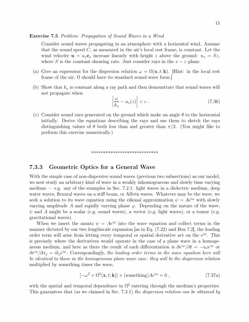
Exercise 7.5 Problem: Propagation of Sound Waves in a Wind

Consider sound waves propagating in an atmosphere with a horizontal wind. Assumethat the sound speed C, as measured in the air’s local rest frame, is constant. Let thewind velocity u = uxex increase linearly with height z above the ground: ux = Sz,where S is the constant shearing rate. Just consider rays in the x− z plane.

(a) Give an expression for the dispersion relation ω = Ω(x, t;k). [Hint: in the local restframe of the air, Ω should have its standard sound-wave form.]

(b) Show that kx is constant along a ray path and then demonstrate that sound waves willnot propagate when

∣

∣

∣

∣

ω

kx− ux(z)

∣

∣

∣

∣

< c . (7.36)

(c) Consider sound rays generated on the ground which make an angle θ to the horizontalinitially. Derive the equations describing the rays and use them to sketch the raysdistinguishing values of θ both less than and greater than π/2. (You might like toperform this exercise numerically.)

****************************

7.3.3 Geometric Optics for a General Wave

With the simple case of non-dispersive sound waves (previous two subsections) as our model,we now study an arbitrary kind of wave in a weakly inhomogeneous and slowly time varyingmedium — e.g. any of the examples in Sec. 7.2.1: light waves in a dielectric medium, deepwater waves, flexural waves on a stiff beam, or Alfvén waves. Whatever may be the wave, weseek a solution to its wave equation using the eikonal approximation ψ = Aeiϕ with slowlyvarying amplitude A and rapidly varying phase ϕ. Depending on the nature of the wave,ψ and A might be a scalar (e.g. sound waves), a vector (e.g. light waves), or a tensor (e.g.gravitational waves).

When we insert the ansatz ψ = Aeiϕ into the wave equation and collect terms in themanner dictated by our two lengthscale expansion [as in Eq. (7.22) and Box 7.2], the leadingorder term will arise from letting every temporal or spatial derivative act on the eiϕ. Thisis precisely where the derivatives would operate in the case of a plane wave in a homoge-neous medium, and here as there the result of each differentiation is ∂eiϕ/∂t = −iωeiϕ or∂eiϕ/∂xj = ikje

iϕ. Correspondingly, the leading order terms in the wave equation here willbe identical to those in the homogeneous plane wave case: they will be the dispersion relationmultiplied by something times the wave,

[−ω2 + Ω2(x, t;k)]× (something)Aeiϕ = 0 , (7.37a)

with the spatial and temporal dependence in Ω2 entering through the medium’s properties.This guarantees that (as we claimed in Sec. 7.3.1) the dispersion relation can be obtained by

16

analyzing a plane, monochromatic wave in a homogeneous, time-independent medium andthen letting the medium’s properties, in the dispersion relation, vary slowly with x and t.

Each next-order (“subleading”) term in the wave equation will entail just one of the waveoperator’s derivatives acting on a slowly-varying quantity (A or a medium property or ω ork), and all the other derivatives acting on eiϕ. The subleading terms that interest us, for themoment, are those where the one derivative acts on A thereby propagating it. The subleadingterms, therefore, can be deduced from the leading-order terms (7.37a) by replacing just oneiωAeiϕ = −A(eiϕ),t by −A,te

iϕ, and replacing just one ikjAeiϕ = A(eiϕ),j by A,je

iϕ. A littlethought then reveals that the equation for the vanishing of the subleading terms must takethe form [deducible from the leading terms (7.37a)]

−2iω∂A

∂t− 2iΩ(k,x, t)

∂Ω(k,x, t)

∂kj

∂A

∂xj= terms proportional to A . (7.37b)

Using the dispersion relation ω = Ω(x, t;k) and the group velocity (first Hamilton equation)∂Ω/∂kj = Vg j, we bring this into the “propagate A along a ray” form

dA

dt≡ ∂A

∂t+Vg ·∇A = terms proportional to A . (7.37c)

Let us return to the leading order terms (7.37a) in the wave equation, i.e. to the dispersionrelation ω = Ω(x, t; k). For our general wave, as for the prototypical dispersionless wave ofthe previous two sections, the argument embodied in Eqs. (7.26) shows that the rays aredetermined by Hamilton’s equations (7.25),

dxjdt

=

(

∂Ω

∂kj

)

x,t

≡ Vg j ,dkjdt

= −(

∂Ω

∂xj

)

k,t

,dω

dt=

(

∂Ω

∂t

)

x,k

, (7.38)

but using the general wave’s dispersion relation Ω(k,x, t) rather than Ω = C(x, t)k. TheseHamilton equations include propagation laws for ω = −∂ϕ/∂t and kj = ∂ϕ/∂xj , from whichwe can deduce the propagation law (7.27) for ϕ along the rays

dϕ

dt= −ω +Vg · k . (7.39)

For waves with dispersion, by contrast with sound in a fluid and other waves that haveΩ = Ck, ϕ will not be constant along a ray.

For our general wave, as for dispersionless waves, the Hamilton equations for the rayscan be reinterpreted as Hamilton’s equations for the world lines of the waves’ quanta [Eq.(7.30) and associated discussion]. And for our general wave, as for dispersionless waves,the medium’s slow variations are incapable of creating or destroying wave quanta. [This isa general feature of quantum theory; creation and destruction of quanta require imposedoscillations at the high frequency and short wavelength of the waves themselves, or at somesubmultiple of them (in the case of nonlinear creation and annihilation processes; Chap.10).] Correspondingly, if one knows the relationship between the waves’ energy density U

17

and their amplitude A, and thence the relationship between the waves’ quantum numberdensity n = U/~ω and A, then from the quantum conservation law [boxed Eqs. (7.34)]

∂n

∂t+∇ · (nVg) = 0 or

dn

dt+ n∇ ·Vg = 0 or

d(nCA)

dt= 0 (7.40)

one can deduce the propagation law for A — and the result must be the same propagationlaw as one obtains from the subleading terms in the eikonal approximation.

7.3.4 Examples of Geometric-Optics Wave Propagation

Spherical scalar waves.As a simple example of these geometric-optics propagation laws, consider a scalar wave

propagating radially outward from the origin at the speed of light in flat spacetime. Settingthe speed of light to unity, the dispersion relation is Eq. (7.4) with C = 1: Ω = k. It isstraightforward (Ex 7.6) to integrate Hamilton’s equations and learn that the rays have thesimple form r = t + constant, θ = constant, φ = constant, k = ωer in spherical polarcoordinates, with er the unit radial vector. Because the wave is dispersionless, its phase ϕmust be conserved along a ray [Eq. (7.28)], i.e. ϕ must be a function of t− r, θ, φ. In orderthat the waves propagate radially, it is essential that k = ∇ϕ point very nearly radially;this implies that ϕ must be a rapidly varying function of t− r and a slowly varying functionof (θ, φ). The law of conservation of quanta in this case reduces to the propagation lawd(rA)/dt = 0 (Ex. 7.6) so rA is also a constant along the ray; we shall call it B. Puttingthis all together, we conclude that

ψ =B(t− r, θ, φ)

reiϕ(t−r,θ,φ) , (7.41)

where the phase ϕ is rapidly varying in t − r and slowly varying in the angles, and theamplitude is slowly varying in t− r and the angles.

Flexural waves.As another example of the geometric-optics propagation laws, consider flexural waves

on a spacecraft’s tapering antenna. The dispersion relation is Ω = k2√

D/Λ [Eq. (7.6)]with D/Λ ∝ h2, where h is the antenna’s thickness in its direction of bend (or the antenna’sdiameter, if it has a circular cross section); cf. Eq. (12.34). Since Ω is independent of t, as thewaves propagate from the spacecraft to the antenna’s tip, their frequency ω is conserved [thirdof Eqs. (7.38)], which implies by the dispersion relation that k = (D/Λ)−1/4ω1/2 ∝ h−1/2,whence the wavelength decreases as h1/2. The group velocity is Vg = 2(D/Λ)1/4ω1/2 ∝ h1/2.Since the energy per quantum ~ω is constant, particle conservation implies that the waves’energy must be conserved, which in this one-dimensional problem, means that the energyflux must be constant along the antenna. On physical grounds the constant energy flux mustbe proportional to A2Vg, which means that the amplitude A must increase ∝ h−1/4 as theflexural waves approach the antenna’s end. A qualitatively similar phenomenon is seen inthe “cracking” of a bullwhip.

Light through lens, and Alfvén waves

18

(b)

(a)

k

ray

Lens

Planet

Source

φ=const.

φ=const.φ=const.φ = const.

Vg

φ=const.

ray

ray

ray

ray

k

Vg

k

kφ=const.

Fig. 7.3: (a) The rays and the surfaces of constant phase ϕ at a fixed time for light passingthrough a converging lens [dispersion relation Ω = ck/n(x), where n is the index of refraction].In this case the rays (which always point along Vg) are parallel to the wave vector k = ∇ϕ andthus also parallel to the phase velocity Vph, and the waves propagate along the rays with a speedVg = Vph = c/n that is independent of wavelength. The strange self-intersecting shape of the lastphase front is due to caustics; see Sec. 7.5. (b) The rays and surfaces of constant phase for Alfvénwaves in the magnetosphere of a planet [dispersion relation Ω = a(x) · k]. In this case becauseVg = a ≡ B/

√µ0ρ, the rays are parallel to the magnetic field lines and not parallel to the wave

vector, and the waves propagate along the field lines with speeds Vg = B/√µ0ρ that are independent

of wavelength; cf. Fig. 7.2c. As a consequence, if some electric discharge excites Alfvén waves on theplanetary surface, then they will be observable by a spacecraft when it passes magnetic field lines onwhich the discharge occurred. As the waves propagate, because B and ρ are time independent andthence ∂Ω/∂t = 0, the frequency ω and energy ~ω of each quantum is conserved, and conservationof quanta implies conservation of wave energy. Because the Alfvén speed generally diminishes withincreasing distance from the planet, conservation of wave energy typically requires the waves’ energydensity and amplitude to increase as they climb upward.

Fig. 7.3 sketches two other examples: light propagating through a lens, and Alfvén wavespropagating in the magnetosphere of a planet. In Sec. 7.3.6 and the exercises we shallexplore a variety of other applications, but first we shall describe how the geometric-opticspropagation laws can fail (Sec. 7.3.5).

****************************

EXERCISES

Exercise 7.6 Derivation and Practice: Quasi-Spherical Solution to Vacuum Scalar WaveEquation

Derive the quasi-spherical solution (7.41) of the vacuum scalar wave equation −∂2ψ/∂t2+∇2ψ = 0 from the geometric optics laws by the procedure sketched in the text.

19

****************************

7.3.5 Relation to Wave Packets; Breakdown of the Eikonal Approx-

imation and Geometric Optics

The form ψ = Aeiϕ of the waves in the eikonal approximation is remarkably general. Atsome initial moment of time, A and ϕ can have any form whatsoever, so long as the two-lengthscale constraints are satisfied [A, ω ≡ −∂ϕ/∂t, k ≡ ∇ϕ, and dispersion relationΩ(k;x, t) all vary on lengthscales long compared to λ = 1/k and timescales long comparedto 1/ω]. For example, ψ could be as nearly planar as is allowed by the inhomogeneities ofthe dispersion relation. At the other extreme, ψ could be a moderately narrow wave packet,confined initially to a small region of space (though not too small; its size must be largecompared to its mean reduced wavelength). In either case, the evolution will be governedby the above propagation laws.

Of course, the eikonal approximation is an approximation. Its propagation laws makeerrors, though when the two-lengthscale constraints are well satisfied, the errors will besmall for sufficiently short propagation times. Wave packets provide an important example.Dispersion (different group velocities for different wave vectors) causes wave packets to spread(widen; disperse) as they propagate; see Ex. 7.2. This spreading is not included in thegeometric optics propagation laws; it is a fundamentally wave-based phenomenon and is lostwhen one goes to the particle-motion regime. In the limit that the wave packet becomesvery large compared to its wavelength or that the packet propagates for only a short time,the spreading is small (Ex. 7.2). This is the geometric-optics regime, and geometric opticsignores the spreading.

Many other wave phenomena are missed by geometric optics. Examples are diffraction,e.g. at a geometric-optics caustic (Secs. 7.5 and 8.6), nonlinear wave-wave coupling (Chaps.10 and 23, and Sec. 16.3), and parametric amplification of waves by rapid time variations ofthe medium (Sec. 10.6)—which shows up in quantum mechanics as particle production (i.e.,a breakdown of the law of conservation of quanta). In Chap. 28, we shall study such particleproduction in inflationary models of the early universe.

7.3.6 Fermat’s Principle

The Hamilton equations of optics allow us to solve for the paths of rays in media thatvary both spatially and temporally. When the medium is time independent, the rays x(t)can be computed from a variational principle named after Pierre de Fermat. This Fermat’sprinciple is the optical analogue of Maupertuis’ principle of least action in classical mechanics.In classical mechanics, this principle states that, when a particle moves from one point toanother through a time-independent potential (so its energy, the Hamiltonian, is conserved),then the path q(t) that it follows is one that extremizes the action

J =

∫

p · dq , (7.42)

20

(where q, p are the particle’s generalized coordinates and momentum), subject to the con-straint that the paths have a fixed starting point, a fixed endpoint, and constant energy.The proof [which can be found, e.g., in Sec. 8.6 of Goldstein, Safko and Poole (2002)] carriesover directly to optics when we replace the Hamiltonian by Ω, q by x, and p by k. Theresulting Fermat principle, stated with some care, has the following form:

Consider waves whose Hamiltonian Ω(k,x) is independent of time. Choose an initiallocation xinitial and a final location xfinal in space, and ask what are the rays x(t) that connectthese two points. The rays (usually only one) are those paths that satisfy the variationalprinciple

δ

∫

k · dx = 0 . (7.43)

In this variational principle, k must be expressed in terms of the trial path x(t) using Hamil-ton’s equation dxj/dt = −∂Ω/∂kj ; the rate that the trial path is traversed (i.e., the magnitudeof the group velocity) must be adjusted so as to keep Ω constant along the trial path (whichmeans that the total time taken to go from xinitial to xfinal can differ from one trial path toanother); and, of course, the trial paths must all begin at xinitial and end at xfinal.

Notice that, once a ray has been identified via this action principle, it has k = ∇ϕ, andtherefore the extremal value of the action

∫

k · dx along the ray is equal to the waves’ phasedifference ∆ϕ between xinitial and xfinal. Correspondingly, for any trial path we can think ofthe action as a phase difference along that path,

∆ϕ =

∫

k · dx , (7.44a)

and we can think of the action principle as one of extremal phase difference ∆ϕ. Thiscan be reexpressed in a form closely related to Feynman’s path-integral formulationof quantum mechanics: We can regard all the trial paths as being followed with equalprobability; for each path we are to construct a probability amplitude ei∆ϕ; and we mustthen add together these amplitudes

∑

all paths

ei∆ϕ (7.44b)

to get the net complex amplitude for quanta associated with the waves to travel from xinitial

to xfinal. The contributions from almost all neighboring paths will interfere destructively.The only exceptions are those paths whose neighbors have the same values of ∆ϕ, to firstorder in the path difference. These are the paths that extremize the action (7.43); i.e., theyare the wave’s rays, the actual paths of the quanta.

Specialization to Ω = C(x)kFermat’s principle takes on an especially simple form when not only is the Hamilto-

nian Ω(k,x) time independent, but it also has the simple dispersion-free form Ω = C(x)k— a form valid for propagation of light through a time-independent dielectric, and soundwaves through a time-independent, inhomogeneous fluid, and electromagnetic or gravita-tional waves through a time-independent, Newtonian gravitational field (Sec. 7.6). In thisΩ = C(x)k case, the Hamiltonian dictates that for each trial path, k is parallel to dx, andtherefore k · dx = kds, where s is distance along the path. Using the dispersion relation

21

k = Ω/C and noting that Hamilton’s equation dxj/dt = ∂Ω/∂kj implies ds/dt = C for therate of traversal of the trial path, we see that k · dx = kds = Ωdt. Since the trial paths areconstrained to have Ω constant, Fermat’s principle (7.43) becomes a principle of extremaltime: The rays between xinitial and xfinal are those paths along which

∫

dt =

∫

ds

C(x)=

∫

n(x)

cds (7.45)

is extremal. In the last expression we have adopted the convention used for light in a dielectricmedium, that C(x) = c/n(x), where c is the speed of light in vacuum and n is the medium’sindex of refraction. Since c is constant, the rays are paths of extremal optical path length∫

n(x)ds.We can use Fermat’s principle to demonstrate that, if the medium contains no opaque

objects, then there will always be at least one ray connecting any two points. This is becausethere is a lower bound on the optical path between any two points given by nminL, wherenmin is the lowest value of the refractive index anywhere in the medium and L is the distancebetween the two points. This means that for some path the optical path length must be aminimum, and that path is then a ray connecting the two points.

From the principle of extremal time, we can derive the Euler-Lagrange differential equa-tion for the ray. For ease of derivation, we write the action principle in the form

δ

∫

n(x)

√

dx

ds· dxds

ds, (7.46)

where the quantity in the square root is identically one. Performing a variation in the usualmanner then gives

d

ds

(

n

dx

ds

)

= ∇n , i.e.d

ds

(

1

C

dx

ds

)

= ∇

(

1

C

)

. (7.47)

This is equivalent to Hamilton’s equations for the ray, as one can readily verify using theHamiltonian Ω = kc/n (Ex. 7.7).

Equation (7.47) is a second-order differential equation requiring two boundary conditionsto define a solution. We can either choose these to be the location of the start of the ray andits starting direction, or the start and end of the ray. A simple case arises when the medium isstratified, i.e. when n = n(z), where (x, y, z) are Cartesian coordinates. Projecting Eq. (7.47)perpendicular to ez, we discover that ndy/ds and ndx/ds are constant, which implies

n sin θ = constant , (7.48)

where θ is the angle between the ray and ez. This is Snell’s law of refraction. Snell’s law isjust a mathematical statement that the rays are normal to surfaces (wavefronts) on whichthe eikonal (phase) ϕ is constant (cf. Fig. 7.4).

****************************

EXERCISES

22

Exercise 7.7 Derivation: Hamilton’s Equations for Dispersionless Waves; Fermat’s Prin-ciple

Show that Hamilton’s equations for the standard dispersionless dispersion relation (7.4)imply the same ray equation (7.47) as we derived using Fermat’s principle.

Exercise 7.8 Example: Self-Focusing Optical Fibers

Optical fibers in which the refractive index varies with radius are commonly used totransport optical signals. Provided that the diameter of the fiber is many wavelengths,we can use geometric optics. Let the refractive index be

n = n0(1− α2r2)1/2 , (7.49a)

where n0 and α are constants and r is radial distance from the fiber’s axis.

(a) Consider a ray that leaves the axis of the fiber along a direction that makes a smallangle θ to the axis. Solve the ray transport equation (7.47) to show that the radius ofthe ray is given by

r =sin θ

α

∣

∣

∣sin( αz

cos θ

)∣

∣

∣, (7.49b)

where z measures distance along the fiber.

(b) Next consider the propagation time T for a light pulse propagating along a long lengthL of fiber. Show that

T =n0L

c[1 +O(θ4)] , (7.49c)

and comment on the implications of this result for the use of fiber optics for commu-nication.

k n2

θ1

θ1

θ2

k

n1

ϕ=const.

2

1

ez

θ2

λ1

2λ

Fig. 7.4: Illustration of Snell’s law of refraction at the interface between two media where therefractive indices are n1, and n2 (assumed less than n1). As the wavefronts must be continuousacross the interface, simple geometry tells us that λ1/ sin θ1 = λ2/ sin θ2. This and the fact thatthe wavelengths are inversely proportional to the refractive index, λj ∝ 1/nj , imply that n1 sin θ1 =n2 sin θ2, in agreement with Eq. (7.48).

23

Exercise 7.9 *** Example: Geometric Optics for the Schrödinger EquationConsider the non-relativistic Schrödinger equation for a particle moving in a time-dependent,3-dimensional potential well:

−~

i

∂ψ

∂t=

[

1

2m

(

~

i∇)2

+ V (x, t)

]

ψ . (7.50)

(a) Seek a geometric optics solution to this equation with the form ψ = AeiS/~, where A andV are assumed to vary on a lengthscale L and timescale T long compared to those, 1/kand 1/ω, on which S varies. Show that the leading order terms in the two-lengthscaleexpansion of the Schrödinger equation give the Hamilton-Jacobi equation

∂S

∂t+

1

2m(∇S)2 + V = 0 . (7.51a)

Our notation ϕ ≡ S/~ for the phase ϕ of the wave function ψ is motivated by thefact that the geometric-optics limit of quantum mechanics is classical mechanics, andthe function S = ~ϕ becomes, in that limit, “Hamilton’s principal function,” whichobeys the Hamilton-Jacobi equation.5 [Hint: Use a formal parameter σ to keep trackof orders (Box 7.2), and argue that terms proportional to ~

n are of order σn. Thismeans there must be factors of σ in the Schrödinger equation (7.50) itself.]

(b) From Eq. (7.51a) derive the equation of motion for the rays (which of course is identicalto the equation of motion for a wave packet and therefore is also the equation of motionfor a classical particle):

dx

dt=

p

m,

dp

dt= −∇V , (7.51b)

where p = ∇S.

(c) Derive the propagation equation for the wave amplitude A and show that it implies

d|A|2dt

+ |A|2∇ · pm

= 0 . (7.51c)

Interpret this equation quantum mechanically.

****************************

7.4 Paraxial Optics

It is quite common in optics to be concerned with a bundle of rays that are almost parallel,i.e. for which the angle the rays make with some reference ray can be treated as small. Thisapproximation is called paraxial optics, and it permits one to linearize the geometric optics

5See, e.g., Chap. 10 of Goldstein, Safko and Poole.

24

z = 0

1

2z = 3

ex

exex ex

reference

ra

y

ray

Fig. 7.5: A reference ray (thick curve), parameterized by distance z along it, and with a parallel-transported transverse unit basis vector ex that delineates a slowly changing transverse x axis.Other rays, such as the thin curve, are identified by their transverse distances x(z) and y(z), alongex and ey (not shown).

equations and use matrix methods to trace their rays. The resulting matrix formalismunderlies the first order theory of simple optical instruments, e.g. the telescope and themicroscope.

We shall develop the paraxial optics formalism for waves whose dispersion relation hasthe simple, time-independent, nondispersive form Ω = kc/n(x). This applies to light in adielectric medium — the usual application. As we shall see below, it also applies to chargedparticles in a storage ring or electron microscope (Sec. 7.4.2) and to light being lensed by aweak gravitational field (Sec. 7.6).

We start by linearizing the ray propagation equation (7.47). Let z measure distance alonga reference ray. Let the two dimensional vector x(z) be the transverse displacement of someother ray from this reference ray, and denote by (x, y) = (x1, x2) the Cartesian componentsof x, with the transverse Cartesian basis vectors ex and ey transported parallely along thereference ray6 (Fig. 7.5).

Under paraxial conditions, |x| is small compared to the z-lengthscales of the propagation,so we can Taylor expand the refractive index n(x, z) in (x1, x2):

n(x, z) = n(0, z) + xin,i(0, z) +1

2xixjn,ij(0, z) + . . . . (7.52a)

Here the subscript commas denote partial derivatives with respect to the transverse coor-dinates, n,i ≡ ∂n/∂xi. The linearized form of the ray propagation equation (7.47) is thengiven by

d

dz

(

n(0, z)dxidz

)

= n,i(0, z) + xjn,ij(0, z) . (7.52b)

Unless otherwise stated, we restrict ourselves to aligned optical systems in which there isa particular choice of reference ray called the optic axis, for which the term n,i(0, z) on theright hand side of Eq. (7.52b) vanishes, and we choose the reference ray to be the optic axis.Then Eq. (7.52b) is a linear, homogeneous, second-order equation for x(z),

(d/dz)(ndxi/dz) = xjn,ij . (7.53)

Here n and n,ij are evaluated on the reference ray. It is helpful to regard z as “time” andthink of Eq. (7.53) as an equation for the two dimensional motion of a particle (the ray) in a

6By parallel transport, we mean this: the basis vector ex is carried a short distance along the referenceray, keeping it parallel to itself. Then, if the reference ray has bent a bit, ex is projected into the new planethat is transverse to the ray.

25

quadratic potential well. We can solve Eq. (7.53) given starting values x(z′), x(z′) where thedot denotes differentiation with respect to z, and z′ is the starting location. The solutionat some later point z is linearly related to the starting values. We can capitalize on thislinearity by treating x(z), x(z) as a 4 dimensional vector Vi(z), with

V1 = x, V2 = x, V3 = y, V4 = y , (7.54a)

and embodying the linear transformation [linear solution of Eq. (7.53)] from location z′ tolocation z in a transfer matrix Jab(z, z

′):

Va(z) = Jab(z, z′) · Vb(z′) . (7.54b)

The transfer matrix contains full information about the change of position and direction ofall rays that propagate from z′ to z. As is always the case for linear systems, the transfermatrix for propagation over a large interval, from z′ to z, can be written as the product ofthe matrices for two subintervals, from z′ to z′′ and from z′′ to z:

Jac(z, z′) = Jab(z, z

′′)Jbc(z′′, z′) . (7.54c)

7.4.1 Axisymmetric, Paraxial Systems; Lenses, Mirrors, Telescope,

Microscope and Optical Cavity

If the index of refraction is everywhere axisymmetric, so n = n(√

x2 + y2, z), then there isno coupling between the motions of rays along the x and y directions, and the equations ofmotion along x are identical to those along y. In other words, J11 = J33, J12 = J34, J21 = J43,and J22 = J44 are the only nonzero components of the transfer matrix. This reduces thedimensionality of the propagation problem from 4 dimensions to 2: Va can be regarded aseither x(z), x(z) or y(z), y(z), and in both cases the 2 × 2 transfer matrix Jab is thesame.

Let us illustrate the paraxial formalism by deriving the transfer matrices of a few simple,axisymmetric optical elements. In our derivations it is helpful conceptually to focus on raysthat move in the x-z plane, i.e. that have y = y = 0. We shall write the 2-dimensional Vi asa column vector

Va =

(

xx

)

. (7.55a)

The simplest case is a straight section of length d extending from z′ to z = z′ + d. Thecomponents of V will change according to

x = x′ + x′d ,

x = x′ ,

so

Jab =

(

1 d0 1

)

for straight section of length d , (7.55b)

26

u v

Lens

Source

Fig. 7.6: Simple converging lens used to illustrate the use of transfer matrices. The total transfermatrix is formed by taking the product of the straight section transfer matrix with the lens matrixand another straight section matrix.

where x′ = x(z′) etc. Next, consider a thin lens with focal length f . The usual conventionin optics is to give f a positive sign when the lens is converging and a negative sign whendiverging. A thin lens gives a deflection to the ray that is linearly proportional to its dis-placement from the optic axis, but does not change its transverse location. Correspondingly,the transfer matrix in crossing the lens (ignoring its thickness) is:

Jab =

(

1 0−f−1 1

)

for thin lens with focal length f . (7.55c)

Similarly, a spherical mirror with radius of curvature R (again adopting a positive sign for aconverging mirror and a negative sign for a diverging mirror) has a transfer matrix

Jab =

(

1 0−2R−1 1

)

for spherical mirror with radius of curvature R . (7.55d)

As a simple illustration, we consider rays that leave a point source which is located adistance u in front of a converging lens of focal length f , and we solve for the ray positions adistance v behind the lens (Fig. 7.6). The total transfer matrix is the transfer matrix (7.55b)for a straight section, multiplied by the product of the lens transfer matrix (7.55c) and asecond straight-section transfer matrix:

Jab =

(

1 v0 1

)(

1 0−f−1 1

)(

1 u0 1

)

=

(

1− vf−1 u+ v − uvf−1

−f−1 1− uf−1

)

. (7.56)

When the 1-2 element (upper right entry) of this transfer matrix vanishes, the positionof the ray after traversing the optical system is independent of the starting direction. Inother words, rays from the point source form a point image. When this happens, the planescontaining the source and the image are said be conjugate. The condition for this to occur is

1

u+

1

v=

1

f. (7.57)

27

This is the standard thin-lens equation. The linear magnification of the image is given byM = J11 = 1− v/f , i.e.

M = −vu, (7.58)

where the negative sign means that the image is inverted. Note that, if a ray is reversed indirection, it remains a ray, but with the source and image planes interchanged; u and v areexchanged, Eq. (7.57) is unaffected, and the magnification (7.58) is inverted: M → 1/M.

****************************

EXERCISES

Exercise 7.10 Problem: Matrix Optics for a Simple Refracting Telescope

Consider a simple refracting telescope (Fig. 7.7) that comprises two converging lenses, theobjective and the eyepiece. This telescope takes parallel rays of light from distant stars,which make an angle θ ≪ 1 with the optic axis, and converts them into parallel rays makinga much larger angle Mθ. Here M is the magnification with M negative, |M| ≫ 1 and|Mθ| ≪ 1. (The parallel output rays are then focused by the lens of a human’s eye, to apoint on the eye’s retina.)

(a) Use matrix methods to investigate how the output rays depend on the separation ofthe two lenses and hence find the condition that the output rays are parallel when theinput rays are parallel.

(b) How does the magnification M depend on the ratio of the focal lengths of the twolenses?

(c) If, instead of looking through the telescope with one’s eye, one wants to record thestars’ image on a photographic plate or CCD, how should the optics be changed?

Mθoptic axis

ray

ray

θ

ray ray

objective

eye piece

Fig. 7.7: Simple refracting telescope. By convention θ > 0 and Mθ < 0, so the image is inverted.

28

optic axis rayray

ray

objective

eye piece

Fig. 7.8: Simple microscope.

Exercise 7.11 Problem: Matrix Optics for a Simple Microscope

A microscope takes light rays from a point on a microscopic object, very near the optic axis,and transforms them into parallel light rays that will be focused by a human eye’s lens ontothe eye’s retina. Use matrix methods to explore the operation of such a microscope. Asingle lens (magnifying glass) could do the same job (rays from a point converted to parallelrays). Why does a microscope need two lenses? What focal lengths and lens separations areappropriate for the eye to resolve a bacterium, 100µm in size?

Exercise 7.12 Example: Optical Cavity – Rays Bouncing Between Two Mirrors

Consider two spherical mirrors, each with radius of curvature R, separated by distance d soas to form an “optical cavity,” as shown in Fig. 7.9. A laser beam bounces back and forthbetween the two mirrors. The center of the beam travels along a geometric-optics ray. (Weshall study such beams, including their diffractive behavior, in Sec. 8.5.5.)

(a) Show, using matrix methods, that the central ray hits one of the mirrors (either one)at successive locations x1,x2,x3 . . . (where x ≡ (x, y) is a 2 dimensional vector in theplane perpendicular to the optic axis), which satisfy the difference equation

xk+2 − 2bxk+1 + xk = 0 (7.59a)

where

b = 1− 4d

R+

2d2

R2. (7.59b)

Explain why this is a difference-equation analogue of the simple-harmonic-oscillatorequation.

x2

x1

x3

Fig. 7.9: An optical cavity formed by two mirrors, and a light beam bouncing back and forthinside it.

29

(b) Show that this difference equation has the general solution

xk = A cos(k cos−1 b) +B sin(k cos−1 b) . (7.59c)

Obviously, A is the transverse position x0 of the ray at its 0’th bounce. The ray’s 0’thposition x0 and its 0’th direction of motion x0 together determine B.

(c) Show that if 0 ≤ d ≤ 2R, the mirror system is “stable”. In other words, all rays oscillateabout the optic axis. Similarly, show that if d > 2R, the mirror system is unstable andthe rays diverge from the optic axis.

(d) For an appropriate choice of initial conditions x0 and x0, the laser beam’s successivespots on the mirror lie on a circle centered on the optic axis. When operated in thismanner, the cavity is called a Harriet delay line. How must d/R be chosen so that thespots have an angular step size θ? (There are two possible choices.)

****************************

7.4.2 Converging Magnetic Lens for Charged Particle Beam

Since geometric optics is the same as particle dynamics, matrix equations can be used todescribe paraxial motions of electrons or ions in a storage ring. (Note, however, that theHamiltonian for such particles is dispersive, since the Hamiltonian does not depend linearlyon the particle momentum, and so for our simple matrix formalism to be valid, we mustconfine attention to a mono-energetic beam of particles.)

S N

N S

ey

ex

Fig. 7.10: Quadrupolar Magnetic Lens. The magnetic field lines lie in a plane perpendicular tothe optic axis. Positively charged particles moving along ez are converged when y = 0 and divergedwhen x = 0.

30

The simplest practical lens for charged particles is a quadrupolar magnet. Quadrupolarmagnetic fields are used to guide particles around storage rings. If we orient our axesappropriately, the magnet’s magnetic field can be expressed in the form

B =B0

r0(yex + xey) independent of z within the lens (7.60)

(Fig. 7.10). Particles traversing this magnetic field will be subjected to a Lorentz forcewhich will curve their trajectories. In the paraxial approximation, a particle’s coordinateswill satisfy the two differential equations

x = − x

λ2, y =

y

λ2, (7.61a)

where the dots (as above) mean d/dz = v−1d/dt and

λ =

(

pr0qB0

)1/2

, (7.61b)

with q the particle’s charge (assumed positive) and p its momentum. The motions in the xand y directions are decoupled. It is convenient in this case to work with two 2-dimensionalvectors, Vx1, Vx2 ≡ x, x and Vy1, Vy2 = y, y. From the elementary solutions to theequations of motion (7.61a), we infer that the transfer matrices from the magnet’s entranceto its exit are Jxab, Jy ab, where

Jxab =

(

cosφ λ sinφ−λ−1 sinφ cos φ

)

, (7.62a)

Jy ab =

(

coshφ λsinhφλ−1sinhφ coshφ

)

, (7.62b)

andφ = L/λ , (7.62c)

with L the distance from entrance to exit (i.e. the lens thickness).The matrices Jx ab, Jy ab can be decomposed as follows

Jxab =

(

1 λ tanφ/20 1

)(

1 0− sin φ/λ 1

)(

1 λ tanφ/20 1

)

(7.62d)

Jy ab =

(

1 λtanhφ/20 1

)(

1 0sinhφ/λ 1

)(

1 λtanhφ/20 1

)

(7.62e)

Comparing with Eqs. (7.55b), (7.55c), we see that the action of a single magnet is equivalentto the action of a straight section, followed by a thin lens, followed by another straightsection. Unfortunately, if the lens is focusing in the x direction, it must be de-focusingin the y direction and vice versa. However, we can construct a lens that is focusing alongboth directions by combining two magnets that have opposite polarity but the same focusingstrength φ = L/λ:

31

Consider first the particles’ motion in the x direction. Let

f+ = λ/ sinφ and f− = −λ/sinhφ (7.63)

be the equivalent focal length of the first converging lens and the second diverging lens. Ifwe separate the magnets by a distance s, this must be added to the two effective lengths ofthe two magnets to give an equivalent separation, d = λ tan(φ/2) + s + λtanh(φ/2) for thetwo equivalent thin lenses. The combined transfer matrix for the two thin lenses separatedby this distance d is then

(

1 0−f−1

− 1

)(

1 d0 1

)(

1 0−f−1

+ 1

)

=

(

1− df−1+ d

−f−1∗

1− df−1−

)

, (7.64a)

where1

f∗=

1

f−+

1

f+− d

f−f+=

sinφ

λ− sinhφ

λ+d sinφ sinhφ

λ2. (7.64b)

If we assume that φ ≪ 1 and s≪ L, then we can expand as a Taylor series in φ to obtain

f∗ ≃3λ

2φ3=

3λ4

2L3. (7.65)

The effective focal length f∗ of the combined magnets is positive and so the lens has a netfocusing effect. From the symmetry of Eq. (7.64b) under interchange of f+ and f−, it shouldbe clear that f∗ is independent of the order in which the magnets are encountered. Therefore,if we were to repeat the calculation for the motion in the y direction, we would get the samefocusing effect. (The diagonal elements of the transfer matrix are interchanged, but as theyare both close to unity, this is a rather small difference.)

The combination of two quadrupole lenses of opposite polarity can therefore imitate theaction of a converging lens. Combinations of magnets like this are used to collimate particlebeams in storage rings, particle accelerators, and electron microscopes.

7.5 Catastrophe Optics — Multiple Images; Formation

of Caustics and their Properties

Many simple optical instruments are carefully made so as to form point images from pointsources. However, naturally occuring optical systems, and indeed precision optical instru-ments, when examined in fine detail, bring light to a focus not at a point, but instead on a2-dimensional (2D) surface in 3D space, called a caustic.7 Caustics are often seen in everydaylife. For example, when when sunlight is refracted by the wavy water on the surface of aswimming pool, its rays form a complex pattern of 2D caustics which intersect the pool’s 2Dbottom in bright lines (Fig. 7.11a). And when sunlight passes through a glass of water (Fig.7.11b), it produces 2D caustics that meet in a line cusp, which intersect a sheet of paper incaustic lines and a point cusp. What may be surprising is that caustics formed under quitegeneral conditions can be classified into a rather small number of types, called catastrophes,

32

including the “fold catastrophes” in Fig. 7.11a, and the “cusp catastrophes” in Fig. 7.11b,and three others. Exercise 7.13 gives some insight into this.

A simple example that is easy to understand analytically occurs when light from a distantsource passes through an imperfect but axisymmetric converging lens; see Fig. 7.12. Herethe caustic is the envelope C of refracted rays (more precisely, the axially symmetric surfaceformed by rotating the curves C around the optic axis). When the light from the lens hitsa screen, it will form a bright circle where the caustic C intersects the screen, analogous tothe bright Caustic lines in Fig. 7.11.

An observer at any point A outside C will see a single image of the source in the directionof the single ray that passes through A; whereas an observer at any point B inside C willsee three images. If the observer at B moves downward toward the caustic, then she willsee two of the images (those along the dotted rays R1 and R2) approach each other, merge,and then vanish, leaving just one ray (the solid line through B) and its image as she movesbeyond C.

This behavior can be understood with the aid of Fermat’s theorem and the constructionin the inset at the right side of Fig. 7.12. Because of axisymmetry, the rays all lie in planesof constant azimuthal angle φ, so we shall focus solely on such a plane — the plane shownin the figure. We choose a point B and characterize it by its longitudinal distance d fromthe lens, and its cylindrical radius . We construct a set of virtual rays8 that hit the lensorthogonally, then bend (at constant φ) and travel straight through B (the solid lines in theinset). We compute the total phase ϕ(b; d,) along each of these virtual rays when it arrives

7See, for example, Berry & Upstill (1980).8A virtual ray is a path that will become a real ray if it satisfies Fermat’s principle.

(a) (b)

Fig. 7.11: Photographs of caustics. (a) Rich pattern of caustics on the bottom of a swimming pool,produced when sunlight passes through the pool’s wavy surface; away from points of intersection,these are fold catastrophes. (b) Two caustics (cusp catastrophes) on a sheet of paper, producedwhen sunlight passes through a water glass. (If the glass were perfectly circularly symmetric insteadof flawed, the cusps would meet at their points.) In both cases the caustic lines shown are crosssections through 2D caustic surfaces, which extend upward from the pool bottom or the sheet ofpaper toward the sun.

33

A

B

C

C

b

Lens

d

R1

R2

virtual rays

ϖb

ϖ

dB

optic axis

Fig. 7.12: The formation of caustics by a thin lens that is constrained to be circularly symmetric.Light from a distant source is refracted at the lens, and in the geometric optics limit, its rays (thearrowed lines, mostly solid but two dotted) bend toward the optic axis as shown. If the lens wereperfect, the rays would all intersect at a point, the lens’s focus. Because it is imperfect, they passthrough the optic axis at different distances from the lens. The caustic C is the envelope of theserays. In the inset labeled “virtual rays”, we show a construction used to explain the caustic. In thisexample, the caustic terminates in a cusp point, which becomes structurally unstable (ceases to bea cusp) if we remove the constraint that the lens be axisymmetric.

at B. (That total ϕ will consist of a phase shift δϕ(b) produced by the lens, plus the phasechange kℓ(b; d,) due to propagation a distance ℓ from the lens to the point of observationB.) By Fermat’s principle, those virtual rays which extremize the total ϕ(b; d,), when b isvaried and d and are held fixed, are the true rays through B.

To understand why, mathematically, there are three real rays [three extrema of ϕ(b; d,)]when B is inside the caustic C and only one when outside, we examine the behavior of ϕas we cross this caustic, i.e. as B’s radius passes through c(d), the radius of the causticat longitudinal location d. From the big diagram in Fig. 7.12, it is clear that, as → c,the two disappearing images (along the dotted rays) approach one another and then vanish.Algebraically, this means that the curves ϕ(b; d,) with fixed observation point (d,) musthave the form shown in Fig. 7.13: as passes through c, a maximum and a minimumsmoothly merge through a point of inflexion and then vanish. It is clear that close enoughto the caustic, ϕ(b; d,), has the form of a cubic:

ϕ(b; d,) =1

3A(b− bc)

3 −B( −c)(b− bc) , (7.66)

where the factor 1/3 is just a convention and bc is some constant. For any given lens, wecan compute the coefficients A, B accurately through a careful Taylor expansion about thecaustic. However, their precise form does not interest us here. Invoking Fermat’s principleand differentiating Eq. (7.66) with respect to b, we see that for < c, there are two truerays and, passing through b−bc = ±[B(−c)/A)

1/2, and two corresponding images; whilefor > c there are no rays or images. [In reality there is another ray, the solid-line ray

34

ϕ

b

φ

b

φ

b

ϖ>ϖc ϖ=0 ϖ<ϖc

Fig. 7.13: Optical phase ϕ for three different near-caustic observer locations , with d fixed. Thetrue rays are refracted at impact parameters b corresponding to extrema of the phase. There aretwo such real rays when the observer lies inside the caustic surface ( < c), and no such real rayswhen she lies outside ( > c). There is a actually one more real ray that is missed here becauseit is at b far from the near-caustic values. For the point B in Fig. 7.12, the real rays captured bythis simple analysis are the dotted ones, and the one missed is the solid one through B.

passing through B in Fig. 7.13. It has been lost from this analysis because we restricted ourmathematics to the vicinity of the disappearing rays when we approximated ϕ as a cubic inb.)

Remarkably, as B approaches the caustic, its two merging images become brighter andbrighter before suddenly disappearing. We can understand this by recalling that, in geometricoptics, a wave’s amplitude varies ∝ 1/(area of a bundle of rays)1/2, so its energy flux varies∝ 1/(bundle’s area). Now consider a ray bundle that hits the lens in the region b to b + dband φ to φ+dφ, and then arrives at B in the range to +d, and (because φ is conservedalong a ray) φ to φ+ dφ. The ratio of the cross sectional areas of this bundle of rays is (areaat lens)/(area at B) = (bdφdb)/dφd = (b/)(db/d) ≡ M; and the observed energyflux is magnified by precisely this factor. As → c, the real rays have b → bc, anddb/d ∝ 1/

√ −c. Therefore, each of the merging images is magnified in energy flux, as

it nears the caustic, by the factor

M ∝ db

d∝ 1√

c −. (7.67)

The scaling law M ∝ 1/√

(distance from caustic) is a general property of fold caustics— equally true for this imperfect lens, for caustics in reflection at a spherical mirror, for thecaustics formed by the rippled surface of the water in a swimming pool (Fig, 7.11a), for thefold portion (not the cusps) of the caustics formed by a water glass (Fig. 7.11), and even forcaustics formed by gravitational lenses (next section). This is just one example of severalscaling laws which apply to caustics.

The theory of optical caustics is a special case of a more general formalism called catas-trophe theory, which deals with boundaries at which smooth behavior ceases and suddenjumps occur. Examples of such catastrophes, in addition to optical caustics, are phase tran-sitions in statistical physics (e.g. Ex. 7.14 below), bifurcation of equilibria in elasticity theory(Sec. 11.8), sudden changes of behavior in nonlinear dynamical systems, and various sudden

35

changes that occur in biological systems and in human enterprises. For discussions see, e.g.,Saunders (1980),

In catastrophe theory, it is shown that there are only a few types of catastrophe and theyhave many generic properties. The key mathematical requirement is that the behavior of acatastrophe should (by definition of “catastrophe”) be structurally stable. This means that,if we make small changes in the physical conditions, its scaling laws etc. are robust.

The caustic that we have just considered is the most elementary example of a catastropheand is called the fold. The next simplest catastrophe, known as the cusp, is the curve in3D where two fold catastrophes meet. (The point cusp displayed in Fig. 7.13, is actuallystructurally unstable as a consequence of the assumed strict axisymmetry. However if band were 1D Cartesian coordinates rather than cylindrical radii, then Fig. 7.13 wouldstill correctly depict the rays’ and caustic’s geometry, and its cusp catastrophe would bestructurally stable; it would be the cusp in the picture, extending into the picture to formtwo intersecting surfaces.)

In total there are five elementary catastrophes, when one deals with a two-parameterfamily of time-independent optical rays in three dimensions—for example, the rays from adistant point source of light that pass through a phase-shifting surface or thin layer, e.g.an imperfect lens or the wavy surface of a swimming pool. If the incoming light hits thesurface orthogonally (for simplicity) and δϕ(a, b) is the phase shift produced by the surface atCartesian-coordinate-location (a, b), and if the observation point is at Cartesian-coordinate-location (x, y, z) a distance ℓ(a, b; x, y, z) from point (a, b) on the surface, then the phase ofthe light arriving along a straight-line virtual ray from (a, b) to (x, y, z) is ϕ(a, b; x, y, z) =δϕ(a, b) + kℓ(a, b; x, y, z). In the vicinity of a structurally stable caustic, a thereom due toRéné Thom says that that there are only five possible independent functional forms for thisϕ(a, b; x, y, z) (see Ex. 7.13) and they lead to the five caustic structures (catastrophes) shownin Fig. 7.14. If one adds a fourth dimension (e.g., time), then there are seven elementarycatastrophes.

We conclude with a very important remark. If we have a point source of light, geometricoptics predicts that the magnification will diverge to infinity as any caustic is approached,e.g. for a fold caustic, as M ∝ 1/

√distance from caustic [Eq. (7.67)]. Two factors prevent

the magnification from becoming truly infinite. The first is that a point source is onlyan idealization, and if we allow the source to have finite size, different parts will producecaustics at slightly different locations. The second is that geometric optics, on which ouranalysis was based, pretends that the wavelength of light is vanishingly small. In actuality,the wavelength is always nonzero, and near a caustic its finiteness leads to diffraction effects,which limit the magnification to a finite value (Sec. 8.6). Diffraction is the subject of thenext chapter.

****************************

EXERCISES

Exercise 7.13 **Example: The Five Catastrophes in OpticsConsider any two-parameter family of virtual light rays arriving, with phase ϕ, at an ob-servation point near a caustic in 3-dimensional space. Denote by (ξ1, ξ2) = (a, b) the ray

36

fold cusp swallowtail

hyperbolic umbilic elliptic umbilic

x

yz

xy

z

x

y

z

Fig. 7.14: The five elementary catastrophes (caustic structures) that are possible for a 2-parameterset of light rays in 3-dimensional space. For the three most complicated catastrophes, we show twodepictions. When the light hits a screen, all bright caustic lines on the screen are made up oftwo-dimensional cross sections of these caustics. All drawings are adapted from Berry and Upstill(1980) or from an unpublished poster by Michael Berry: http://www.phy.bris.ac.uk/people/

berry_mv/pictures/poster1.pdf .

parameters (called state variables in catastrophe theory), and by (x1, x2, x3) = (x, y, z) theCartesian coordinates of the observation point, so the arriving light’s phase is ϕ(a, b, ; x, y, z).In this exercise we shall explore the five possible functional forms of this phase near a caus-tic, as identified by Thom’s theorem, and their consequences for the caustic’s (catastrophe’s)structure..

(a) The Fold Catastrophe. Very near a fold catastrophe (caustic), with an appropriateparametrization and choice of coordinates (including absorbing some constants intoa, b, z, y, z), the light’s phase function is

ϕ =1

3b3 − xb . (7.68)

Notice that this is identical to the phase near the caustic of the lens treated in the text(Fig. 7.13): it is the same as Eq. (7.66) with A = B = 1, bc = c = 0 and = −x. Inthis case, the phase is independent of a, y, z. (i) Following the procedure used in thetext, infer from Fermat’s principle that the rays (if any) that pass through location xhave b = ±√

x. This is the ray map in the language of optics; it maps the observationallocation x onto the values of b that label the real rays passing through x. (ii) Depictthe ray map by plotting b upward and x horizontally, restricting attention to real band x since by definition both must be real. This equilibrium surface (as it is calledin catastrophe theory) folds over at x = 0, which is why this catastrophe is called the

37

fold. (iii) As this plot and its equation b = ±√x show, there are two rays (two values

of b) for x > 0 and none for x < 0. Therefore, x = 0 — the location of the fold — isthe caustic for all y, z, which means that the caustic is a plane as depicted in Fig. 7.14.

(b) The Cusp Catastrophe. For the cusp catastrophe, the phase function is

ϕ =1

4b4 − 1

2xb2 − yb . (7.69)

Because ϕ is independent of z, the caustic will be translation invariant in the z direc-tion. (i) From Fermat’s principle infer that the ray map (equilibrium surface) is theset of solutions b(x, y) to the equation b3−xb− y = 0. Because this is a cubic in b andrays can only be created and disappear in pairs, there will be some regions of spacethrough which pass three rays, and some, one. (ii) Plot the equilibrium surface b(x, y)(using a computer). From the plot, identify visually the region with three rays and theregion with one, and the caustic that separates them. (iii) Show analytically that thecaustic is the cusp y = ±2(x/3)3/2. Verify visually that this agrees with your plot in(ii), and with the shape depicted in Fig. 7.14.

(c) The Swallowtail Catastrophe. For the swallowtail catastrophe, the phase functionis

ϕ =1

5b5 − 1

3xb3 − 1

2yb2 − zb . (7.70)

(i) From Fermat’s principle infer that the ray map is the set of solutions b(x, y, z) tothe equation b4 − xb2 − yb− z = 0. Because this is a quartic, there can be regions ofspace with 4, 2, and 0 rays passing through each event. It is not practical to plot the“equilibrium surface” b(x, y, z), since that would be a four dimensional plot. (ii) Showthat the caustic, at which the number of rays changes, is given by z = b4−xb2−yb withb(x, y) the solution to 4b3 − 2xb − y = 0. Draw this caustic surface with a computerand verify that it agrees with the swallowtail shown in Fig. 7.14.

(d) The Hyperbolic Umbilic Catastrophe. For the hyperbolic umbilic catastrophe, thephase function depends on two ray parameters ξ1 = a, ξ2 = b, and on all three spatialcoordinates x, y, z:

ϕ =1

3(a3 + b3)− zab− xa− yb . (7.71)

(i) Explain why Fermat’s principle dictates that the ray map be given by ∂ϕ/∂ξj = 0,which is two equations. Show that the resulting ray map a(x, y, z), b(x, y, z) is givenby the solution to a2 − zb − x = 0 and b2 − za − y = 0. (ii) Explain why thecaustic — the points in space at which the number of rays changes by two — is givenby eliminating the parameters ξi from the following three equations: ∂ϕ/∂ξi = 0 anddet[∂2ϕ/∂ξi∂ξj ] = 0. Show that these three equations are a2−zb−x = 0, b2−za−y = 0,and 4ab − z2 = 0, with a and b to be eliminated. Plot the resulting z(x, y) and showthat it agrees with the hyperbolic umbilic shape depicted in Fig. 7.14

38

(e) The Elliptic Umbilic Catastrophe. For the elliptic umbilic catastrophe, the phasefunction is:

ϕ =1

3a3 − ab2 − z(a2 + b2)− xa− yb . (7.72)

Following the procedure developed in part (d), show that the caustic is the functionz(x, y) obtained by eliminating a and b from the three equations a2− b2−x−2za = 0,2ab + y + 2zb = 0, and b2 + a2 − z2 = 0. Plot the resulting z(x, y) and show that itagrees with the elliptic umbilic shape depicted in Fig. 7.14

Exercise 7.14 **Example: Van der Waals Catastrophe

The van der Waals equation of state (P +a/v2)(v− b) = kBT for H2O relates the pressure Pand specific volume (volume per molecule) v to the temperature T ; see Sec. 5.7. Figure 5.8makes it clear that, at some temperatures and pressures T and P , there are three allowedvolumes v(T, P ), one describing liquid water, one water vapor, and the third an unstablephase that cannot exist in Nature. At other T , P , there is only one allowed v. The transitionbetween three v’s and one occurs along some curve in the T , P plane—a catastrophe curve.

(a) This curve must correspond to one of the elementary catastrophes explored in theprevious exercise. Based on the number of solutions for v(T, P ), which catastrophemust it be?

(b) Change variables, in the van der Waals equation of state, to p = P/Pc−1, t = T/Tc−1,ρ = Vc/V − 1, where Tc = 8a/27bkB, Pc = a/27b2, vc = 3b are the temperature,pressure, and specific volume at the critical temperature (the temperature below whichliquid water and water vapor can exist as separate phases; Sec. 5.7). Show that thischange of variables brings the van der Waals equation of state into the form

ρ3 − xρ− y = 0 , where x = −(p/3 + 8t/3) , y = 2p/3− 8t/3 . (7.73)

(c) This equation ρ3 − xρ − y is the equilibrium surface associated with the catastrophe-theory potential ϕ(ρ; x, y) = 1

4ρ4 − 1

2xρ2 − yρ [Eq. (7.69)]. Correspondingly, the catas-

trophe [the boundary between three solutions v(T, P ) and one] has the universal cuspform x = ±2(y/3)2/3. Plot this curve in the temperature-pressure plane.

Note: We were guaranteed by catastrophe theory that the catastrophe curve would have thiscusp form near its cusp point. However, it is a surprise and quite unusual that, for the vander Waals case, the cusp shape x = ±2(y/3)2/3 is not confined to the vicinity of the cusppoint, but remains accurate far from the cusp point.

****************************

39

7.6 T2 Gravitational Lenses; Their Multiple Images and

Caustics

Albert Einstein’s general relativity theory predicts that light rays should be deflected by thegravitational field of the Sun (Ex. 27.3; Sec. 27.2.3). Newton’s law of gravity combined withhis corpuscular theory of light also predicts this deflection, but through an angle half asgreat as relativity predicts. A famous measurement, during a 1919 solar eclipse, confirmedthe relativistic prediction, thereby making Einstein world famous.

The deflection of light by gravitational fields allows a distant galaxy to behave like acrude lens and, in particular, to produce multiple images of a more distant quasar. Manyexamples of this phenomenon have been observed. The optics of these gravitational lensesprovides an excellent illustration of the use of Fermat’s principle.9 We shall explore theseissues in this section.

7.6.1 T2 Refractive-Index Model of Gravitational Lensing

The action of a gravitational lens can only be understood properly using general relativity.However, when the gravitational field is weak, there exists an equivalent Newtonian modelthat is adequate for our purposes. In this model, curved spacetime behaves as if it werespatially flat and endowed with a refractive index given by

n = 1− 2Φ

c2, (7.74)

where Φ is the Newtonian gravitational potential, normalized to vanish far from the sourceof the gravitational field and chosen to have a negative sign (so, e.g., the field at a distancer from a point mass M is Φ = −GM/r). Time is treated in the Newtonian manner in thismodel. In Sec. 27.2.3, we will use a general relativistic version of Fermat’s principle to showthat for static gravitational fields this index-of-refraction model gives the same predictionsas general relativity, up to fractional corrections of order |Φ|/c2, which are . 10−5 for thelensing examples in this chapter.

There is a second Newtonian model that gives the same predictions as this index-of-refraction model, to within its errors, ∼ |Φ|/c2. We deduce it by rewriting the ray equation(7.47) in terms of Newtonian time t using ds/dt = C = c/n:

d2x

dt2= nc2∇n = −∇2Φ . (7.75)

Here in the last expression we have used Eq. (7.74) and have replaced the multiplicativefactor n, in the second expression, by unity, thereby making a fractional error ∼ |Φ|/c2 ofthe same magnitude as the errors in our index-of-refraction model. Equation (7.75) saysthat the photons that travel along rays feel a Newtonian gravitational potential that is twiceas large as the potential felt by low-speed particles; and the photons, moving at a speed thatis c aside from fractional changes of order |Φ|/c2, respond to that doubled Newtonian fieldin the same way as any Newtonian particle would.

9Schneider, Ehlers & Falco (1999).

40

7.6.2 T2 Lensing by a Point Mass

We shall explore the predictions of this model, beginning with gravitational lensing by apoint mass M , with Φ = −GM/r; Fig. 7.15. In this case, there is an obvious optic axis: theline between the earth ⊕ and the lens M ; the index of refraction is axisymmetric aroundthat axis, so the ray from the source Q to earth ⊕ will lie in a plane of constant aziumthalangle φ (and φ + π)—the plane shown in Fig. 7.15. Moreover, the ray will bend near thesource, sharply as seen on the lengthscales used in the figure. Therefore, the point mass’sgravity acts like an axisymmetric phase-shifting surface, i.e. an imperfect axisymmetric lens,in the language of the Sec. 7.5.

Computing the ray (photon trajectory) from Eq. (7.75) with 2Φ = −2GM/r is equivalent,of course, to computing the deflection of a charged particle passing by an oppositely charged,far more massive particle. That computation gives a ray deflection angle

α =4GM

bc2=

−4Φ(r = b)

c2, (7.76a)

where b is the ray’s impact parameter; see Ex. 7.15. For a ray from a distant star, passingclose to the limb of the sun, this deflection is α = 1.75 arc seconds.

In Fig. 7.15, we identify the location of the point source Q by its angle θ′ to the opticaxis, as seen from Earth in the absence of the lensing mass. The lensing pushes the imageaway from the optic axis, to a larger angle θ. Elementary geometry plus Eq. (7.76a) revealsthe following relationship between θ and θ′ (Ex. 7.15):

θ′ = θ − θE2

θ, where θE ≡

√

4Mu

v(u+ v)(7.76b)

is called the Einstein (angular) radius. (Here u and v are the distances shown in Fig. 7.15.)This is a quadratic equation for θ in terms of θ′ and θE , and it has two solutions:

θ± =θ′

2±

√

θE2 +

(

θ′

2

)2

. (7.76c)

The ray shown in Fig. 7.15 produces the image at θ = θ+. A ray, not shown there, whichpasses below the lensing mass M and gets deflected upward, produces a second image, at thenegative (upward sloped) angle θ = θ−. If the source of gravity were extended, rather thanbeing a point mass, there would be a third image, along a ray passing through the source.

Moptic axis

Q

α

θθ'

b

vu

ray

ray

Fig. 7.15: Geometry for gravitational lensing of a point source Q by a point mass M .

41

Fig. 7.16: The Einstein ring LRG 3-757, also called “the cosmic horseshoe”, photographed by theHubble Space Telescope. The ring light comes from a very distant galaxy, with cosmological redshiftz ≃ 2.4. The lensing galaxy is the bright yellow spot at the center of the ring.

As the source Q is moved downward toward the optic axis so θ′ → 0, the two images movetoward ±θE , i.e. opposite edges of a circle with angular radius ΘE ; and by axisymmetry, theimages are then suddenly transformed into a thin ring of light, the so-called Einstein ring.An astronomical photograph of such an Einstein ring is shown in Fig. 7.16. When the sourceis moved onward to negative θ′, the ring breaks back up into two images, again on oppositesides of the former ring, one just outside the ring and the other just inside it.

This behavior is very different from that at a generic caustic (Sec. 7.5), where the imageswould coalesce then disappear. This behavior is not structurally stable; if the axisymmetryis broken, then the behavior will change significantly. Nevertheless, for finite-sized sources oflight and generic sources of gravity (e.g. compact stars or galaxies; next subsection), therecan be structurally stable Einstein rings, as Fig. 7.16 demonstrates.

Suppose that the light source Q is finite in size, as always is the case in Nature. Denoteby ∆Ω′ the solid angle it would subtend as seen from earth in the absence of the lens, andby ∆Ω its solid angle in the lens’s presence. The total energy flux received at earth fromthe image is dE/dtdA = (

∫

Iνdν)∆Ω, where Iν = dE/dtdAdνdΩ is the spectral intensitytraveling along the ray. Kinetic theory tells us that Iν/ν

3 is conserved along the ray (end ofSec. 3.6), and because gravity is weak, so is ν and thence so is

∫

Iνdν = I. In the presenceof the lens, then, the received flux is dE/dtdA = I∆Ω, and in the absence of the lens, itwould be dE/dtdA = I∆Ω′. The ratio of the energy fluxes is the magnification,

M = ∆Ω/∆Ω′ . (7.76d)

This is a very general result, as scrutiny of the derivation shows: it holds true, in the geomtricoptics approximation, whenever the frequencies of photons are the same when they reach anobserver, as when they left their source.

42

We can compute this magnification most easily by focusing not on the lensing of thesource’s total surface, but rather the lensing of an elementary angular element on the surfacewith azimuthal extent dφ and poloidal extent dθ. By axisymmetry around the optic axis, dφis unaffected by the lens, so the magnification is (Ex. 7.15)

M =dΩ

dΩ′=

θ dφ dθ

θ′ dφ dθ′=θ

θ′dθ

dθ′=

1

1− (θE/θ)4. (7.76e)

Here we have used Eq. (7.76b) to express θ′ in terms of θ. The image at θ+ > θE has positivemagnification, which means it has the same parity as the source; the image at θ− < θE hasnegative magnification, which means opposite parity to the source.

Notice that, as the source is moved toward and onto the optic axis, so θ → θE , themagnification diverges. This is a signal that our geometric optics approximation is breakingdown; cf. the last paragraph (before the exercises) of Sec. 7.5. From Eqs. (7.76c) and (7.76e),it can be shown (Ex. 7.15) that the ratio of magnifications of the two images is

R =M+

M−

= −(

θ+θ−

)2

. (7.76f)

****************************

EXERCISES

Exercise 7.15 Derivation: Point-Mass Gravitational Lens

For the point-mass gravitational lens geometry shown in Fig. 7.15, derive Eqs. (7.76). [Inci-dentally, Einstein performed a calculation similar to this, in one of his unpublished notebooks,prior to understanding general relativity.]

****************************

7.6.3 T2 Lensing of a Quasar by a Galaxy

When a distant quasar is lensed by a more nearby galaxy as in Fig. 7.17, the images’ raystypically pass through the galaxy, not around it. We can see this by the following roughestimate: The virial theorem (which says that the kinetic energy of a swarm of stars is halfthe magnitude of its potential energy) tells us that the gravitational potential at a ray’spoint of closest approach to the galaxy center is |Φ| = GM/b ∼ 2 × 3

2σ2. Here σ2 is the

stars’ mean square velocity in one dimension so 32σ2 is their mean kinetic energy per unit

mass. Correspondingly, the deflection angle is α = 4|Φ|/c2 ∼ 12σ2/c2. For typical galaxies,σ ∼ 300 km s−1 and this formula gives α ∼ 1−2 arc sec. Now, the distances u, v are roughlyten billion light years ∼ 1026m and so the transverse displacement of the ray due to thegalaxy is ∼ vα/2 ∼ 3 × 1020m ∼ 30, 000 light years (about the distance of the earth fromthe center of our Milky Way galaxy), which is well within the galaxy. This means that light

43

GQ

u v

α

θθ(v/u) reference ray

virtual rayvirtual ray

Fig. 7.17: Geometry for gravitational lensing of a quasar Q by a large galaxy G.

from a quasar lying behind the galaxy can pass through the outer regions of either side ofthe galaxy. We should then see at least two distinct images of the quasar, separated by anangular distance ∼ 1

2α ∼ 1 arc sec.

We shall now analyze the lensing quantitatively for the geometry of Fig. 7.17.10 As fora point source of gravity, so also for a lensing galaxy, because the distances from galaxyto earth and from galaxy to quasar are so large, the galaxy’s gravity will act like a phaseshifting screen. We shall analyze its influence using Fermat’s principle, in the same way aswe did in Sec. 7.5 for an imperfect lens, which also behaved like a phase shifting screen.

First we trace a ray backward from the observer, in the absence of the intervening galaxy,to the quasar. We call this the reference ray. Next, we reinstate the galaxy and consider avirtual ray8 that extends (backward) at an angle θ (a 2-dimensional vector on the sky) tothe reference ray in a straight line from the earth to the galaxy, where it is deflected alonga straight line to the quasar. The optical phase for light propagating along this virtual raywill exceed that along the reference ray by an amount ∆ϕ called the phase delay. Thereare two contributions to ∆ϕ: First, the geometrical length of the path is longer than thereference ray by an amount (u+ v)vθ2/2u (cf. Fig. 7.17), and thus the travel time is longerby an amount (u+ v)vθ2/2uc. Second, the light is delayed as it passes through the potentialwell by a time

∫

(n−1)ds/c = −2∫

Φds/c3, where ds is an element of length along the path.We can express this second delay as 2Φ2/c

3. Here

Φ2 =

∫

Φds (7.77)

is a two-dimensional (2D) Newtonian potential and can be computed from the 2D Poissonequation

∇2Φ2 = 4πGΣ , where Σ =

∫

ρds (7.78a)

is the surface density of mass in the galaxy integrated along the line of sight.

10In our treatment of this lensing example, we shall ignore complications that arise from the universe’sexpansion and its large scale gravitational fields. However, as we discuss in Chap. 28, the universe is spatiallyflat and so the relation between angles and lengths is Euclidean, as in our refractive-index model. We canalso imagine making the lens observations after the universe has expanded to its present age everywhere,and stopping the expansion then so as to measure the distances u, v. If we use this definition of distances,it turns out that we can ignore cosmological effects in analyzing the optics. Our index-of-refraction model isthen accurate, as in non-cosmological contexts, up to fractional errors ∼ |Φ|/c2.

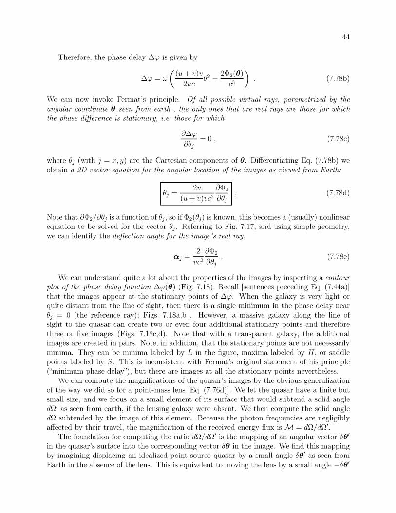
44

Therefore, the phase delay ∆ϕ is given by

∆ϕ = ω

(

(u+ v)v

2ucθ2 − 2Φ2(θ)

c3

)

. (7.78b)

We can now invoke Fermat’s principle. Of all possible virtual rays, parametrized by theangular coordinate θ seen from earth , the only ones that are real rays are those for whichthe phase difference is stationary, i.e. those for which

∂∆ϕ

∂θj= 0 , (7.78c)

where θj (with j = x, y) are the Cartesian components of θ. Differentiating Eq. (7.78b) weobtain a 2D vector equation for the angular location of the images as viewed from Earth:

θj =2u

(u+ v)vc2∂Φ2

∂θj. (7.78d)

Note that ∂Φ2/∂θj is a function of θj , so if Φ2(θj) is known, this becomes a (usually) nonlinearequation to be solved for the vector θj . Referring to Fig. 7.17, and using simple geometry,we can identify the deflection angle for the image’s real ray:

αj =2

vc2∂Φ2

∂θj. (7.78e)

We can understand quite a lot about the properties of the images by inspecting a contourplot of the phase delay function ∆ϕ(θ) (Fig. 7.18). Recall [sentences preceding Eq. (7.44a)]that the images appear at the stationary points of ∆ϕ. When the galaxy is very light orquite distant from the line of sight, then there is a single minimum in the phase delay nearθj = 0 (the reference ray); Figs. 7.18a,b . However, a massive galaxy along the line ofsight to the quasar can create two or even four additional stationary points and thereforethree or five images (Figs. 7.18c,d). Note that with a transparent galaxy, the additionalimages are created in pairs. Note, in addition, that the stationary points are not necessarilyminima. They can be minima labeled by L in the figure, maxima labeled by H , or saddlepoints labeled by S. This is inconsistent with Fermat’s original statement of his principle(“minimum phase delay”), but there are images at all the stationary points nevertheless.

We can compute the magnifications of the quasar’s images by the obvious generalizationof the way we did so for a point-mass lens [Eq. (7.76d)]. We let the quasar have a finite butsmall size, and we focus on a small element of its surface that would subtend a solid angledΩ′ as seen from earth, if the lensing galaxy were absent. We then compute the solid angledΩ subtended by the image of this element. Because the photon frequencies are negligiblyaffected by their travel, the magnification of the received energy flux is M = dΩ/dΩ′.

The foundation for computing the ratio dΩ/dΩ′ is the mapping of an angular vector δθ′

in the quasar’s surface into the corresponding vector δθ in the image. We find this mappingby imagining displacing an idealized point-source quasar by a small angle δθ′ as seen fromEarth in the absence of the lens. This is equivalent to moving the lens by a small angle −δθ′

45

(a) (b)

(c) (d)

LL

LL

LH H

SS

S

Fig. 7.18: Contour plots of the phase delay ∆ϕ(θ) for four different gravitational lenses. (a) In theabsence of a lens Φ2 = 0, the phase delay (7.78b) has a single minimum corresponding to a singleundeflected image, in the direction of the reference ray θj = 0. (b) When a small galaxy with ashallow potential Φ2 is interposed, it pushes the phase delay ∆ϕ up in its vicinity [Eq. (7.78b) withnegative Φ2], so the minimum and hence the image are deflected slightly away from the galaxy’scenter. (c) When a galaxy with a deeper potential well is present, the delay surface will be raisedso much near the galaxy’s center that additional stationary points will be created, at H and S, andtwo more images will be produced. (d) If the potential well deepens even more, five images can beproduced. In all four plots the local extrema of ∆ϕ are denoted L for a low point (local minimum),H for a high point (local maximum) and S for saddle point.

as seen from Earth. Equation (7.78d) says that the image will be displaced by a small angleδθ satisfying the equation

δθi − δθ′i =2u

(u+ v)vc2∂2Φ2

∂θi∂θjδθj . (7.79a)

By combining with Eq. (7.78b), we can rewrite this as

δθ′i = Hijδθj , (7.79b)

where the matrix [Hij] is

Hij =

(

uc/ω

(u+ v)v

)

∂2∆ϕ

∂θi∂θj= δij −

2u

(u+ v)vc2Φ2,ij . (7.79c)

This is the vector mapping we need.It is a standard result in geometry (fairly easily derived) that, because the lensing maps

any δθ′i into δθi = H−1ij δθ

′

j [inverse of the mapping (7.79b)], it maps any infinitesimal solid

46

angle dΩ′ into dΩ = det[H−1ij ]dΩ′ = dΩ′/det[Hij]. Therefore, the flux magnification is

M =dΩ

dΩ′=

1

det [Hij]=

(u+ v)v

uc/ω

1

det [∂2∆ϕ/∂θi∂θj ]] . (7.80)

The curvature of the phase delay surface (embodied in det [∂2∆ϕ/∂θi∂θj ]) is therefore aquantitative measure of the magnification. Small curvature implies large magnification ofthe images and vice versa. Caustics are located where the curvature goes to zero, i.e. wheredet [∂2∆ϕ/∂θi∂θj ] = 0 (cf. Ex. 7.13d). Furthermore, images associated with saddle points inthe phase delay surface have opposite parity to the source. Those associated with maximaand minima have the same parity as the source, although the maxima are rotated on thesky by 180. These effects have been seen in observed gravitational lenses.

There is an additional, immediate contact to the observations and this is that the phasedelay function ∆ϕ at the stationary points is equal to ω times the extra time it takes asignal to arrive along that ray. In order of magnitude, the time delay difference will be∼ vα2/8c ∼ 1 month [cf. Eq. (7.78b)]. Now, many quasars are intrinsically variable, and ifwe monitor the variation in two or more images, then we should be able to measure the timedelay between the two images; cf. Fig. 7.19. This, in turn, allows us to measure the distanceto the quasar and, consequently, provides a measurement of the size of the universe.

****************************

EXERCISES

Exercise 7.16 Challenge: Catastrophe Optics of an Elliptical Gravitational Lens

Consider an elliptical gravitational lens where the potential at the lens plane varies as

Φ2(θ) = (1 + Aθ21 + 2Bθ1θ2 + Cθ22)q; 0 < q < 1/2.

Determine the generic form of the caustic surfaces and the types of catastrophe en-countered. Note that it is in the spirit of catastrophe theory not to compute exactexpressions but to determine scaling laws and to understand the qualitative behaviorof the images.

****************************

7.7 Polarization

In our geometric optics analyses thus far, we have either dealt with a scalar wave (e.g., asound wave) or simply supposed that individual components of vector or tensor waves canbe treated as scalars. For most purposes, this is indeed the case, and we shall continueto use this simplification in the following chapters. However, there are some important

47

Fig. 7.19: Gravitational lens in which a distant quasar, Q1115+080, is quadruply imaged by anintervening galaxy. (There is also a fifth, unseen image.) Two of the images are observed to be muchbrighter and closer to each other than the other two, because the quasar is located quite close to afold caustic surface. When the brightness of the quasar fluctuates, the four images are observed tofluctuate in the order predicted by modeling the gravitational potential of the lensing galaxy, andthese fluctuations can be used to estimate the size of the universe.

wave properties that are unique to vector (or tensor) waves. Most of these come under theheading of polarization effects. In Secs. 27.3 and 27.4, we shall study polarization effects for(tensorial) gravitational waves. Here and in Chaps. 10 and 21–23, we shall examine themfor electromagnetic waves.

An electromagnetic wave’s two polarizations are powerful tools for technology, engineer-ing, and experimental physics. However, we shall forgo any discussion of this in the presentchapter, and instead shall focus solely on the geometric-optics propagation law for polariza-tion (Sec. 7.7.1), and an intriguing aspect of it called the geometric phase (Sec. 7.7.2).

7.7.1 Polarization Vector and its Geometric-Optics Propagation Law

A plane electromagnetic wave in vacuo has its electric and magnetic fields E and B perpen-dicular to its propagation direction k and perpendicular to each other. In a medium, E andB may or may not remain perpendicular to k, depending on the medium’s properties. Forexample, an Alfvén wave has its vibrating magnetic field perpendicular to the backgroundmagnetic field, which can make an arbitrary angle with respect to k. By contrast, in the

48

simplest case of an isotropic dielectric medium, where the dispersion relation has our stan-dard dispersion-free form Ω = (c/n)k, the group and phase velocities are parallel to k, andE and B turn out to be perpendicular to k and to each other—as in vacuum. In this section,we shall confine attention to this simple situation, and to linearly polarized waves, for whichE oscillates linearly back and forth along a polarization direction f that is perpendicular tok:

E = Aeiϕ f , f · k ≡ f ·∇ϕ = 0 . (7.81)

In the eikonal approximation, Aeiϕ ≡ ψ satisfies the geometric-optics propagation lawsof Sec. 7.3, and the polarization vector f , like the amplitude A, will propagate along therays. The propagation law for f can be derived by applying the eikonal approximationto Maxwell’s equations, but it is easier to infer that law by simple physical reasoning: (i)Since f is orthogonal to k for a plane wave, it must also be orthogonal to k in the eikonalapproximation (which, after all, treats the wave as planar on lengthscales long compared tothe wavelength). (ii) If the ray is straight, then the medium, being isotropic, is unable todistinguish a slow right-handed rotation of f from a slow left-handed rotation, so there willbe no rotation at all: f will continue always to point in the same direction, i.e. f will bekept parallel to itself during transport along the ray. (iii) If the ray bends, so dk/ds 6= 0(where s is distance along the ray), then f will have to change as well, so as always to remainperpendicular to k. The direction of f ’s change must be k, since the medium, being isotropic,cannot provide any other preferred direction for the change. The magnitude of the changeis determined by the requirement that f · k remain zero all along the ray and that k · k = 1.This immediately implies that the propagation law for f is

df

ds= −k

(

f · dkds

)

. (7.82)

This equation says that the vector f is parallel-transported along the ray. Here “paralleltransport” means: (i) Carry f a short distance along the ray, keeping it parallel to itself in3-dimensional space. Because of the bending of the ray and its tangent vector k, this willcause f to no longer be perpendicular to k. (ii) Project f perpendicular to k by adding ontoit the appropriate multiple of k. (The techniques of differential geometry for curved linesand surfaces, which we shall develop in Chaps. 24 and 25 in preparation for studying generalrelativity, give powerful mathematical tools for analyzing this parallel transport.)

7.7.2 T2 Geometric Phase

We shall use the polarization propagation law (7.82) to illustrate a quite general phenomenonknown as the geometric phase. For further details and some history of this concept, see Berry(1990).

Consider, as a simple context for the geometric phase, a linearly polarized, monochro-matic light beam that propagates in an optical fiber. Focus on the evolution of the polariza-tion vector along the fiber’s optic axis. We can imagine bending the fiber into any desiredshape, and thereby controlling the shape of the ray. The ray’s shape in turn will control thepropagation of the polarization via Eq. (7.82).

49

If the fiber and ray are straight, then the propagation law (7.82) keeps f constant. Ifthe fiber and ray are circular, then the propagation law (7.82) causes f to rotate in such away as to always point along the generator of a cone, as shown in drawing (a) of Fig. 7.20.This polarization behavior, and that for any other ray shape, can be deduced with the aidof a unit sphere on which we plot the ray direction k [drawing (b)]. For example, the raydirections at ray locations C and H [drawing (a)] are as shown in drawing (b). Notice, thatthe trajectory of k around the unit sphere is a great circle.

On the unit sphere we also plot the polarization vector f — one vector at each pointcorresponding to a ray direction. Because f · k = 0, the polarization vectors are alwaystangent to the unit sphere. Notice that each f on the unit sphere is identical in length anddirection to the corresponding one in the physical space of drawing (a).

The parallel transport law (7.82) keeps constant the angle α between f and the trajectoryof k, i.e. the great circle in drawing (b). Translated back to drawing (a), this constancy ofα implies that the polarization vector points always along the generators of the cone whoseopening angle is π/2− α, as shown.

Next let the fiber and its central axis (the ray) be helical as shown in drawing (a) ofFig. 7.21. In this case, the propagation direction k rotates, always maintaining the sameangle θ to the vertical direction, and correspondingly its trajectory on the unit sphere ofdrawing (b) is a circle of constant polar angle θ. Therefore (as one can see, e.g., with theaid of a large globe of the Earth and a pencil that one transports around a circle of latitude90o − θ), the parallel transport law dictates that the angle α between f and the circle notremain constant, but instead rotate at the rate

dα/dφ = cos θ . (7.83)

Here φ is the angle (longitude on the globe) around the circle. This is the same propagationlaw as for the direction of swing of a Foucault Pendulum as the earth turns, and for the same

Ray

fv f

v

fv

A

ABBCC

DE

HGFD

E F

G

H

(a) (b)

kv

kv

αα

αα

Fig. 7.20: (a) The ray along the optic axis of a circular loop of optical fiber, and the polarizationvector f that is transported along the ray by the geometric-optics transport law df/ds = −k(f ·dk/ds). (b) The polarization vector f drawn on the unit sphere. The vector from the center ofthe sphere to each of the points A, B, ..., is the ray’s propagation direction k, and the polarizationvector (which is orthogonal to k and thus tangent to the sphere) is identical to that in the physicalspace of the ray [drawing (a)].

50

reason: the gyroscopic action of the Foucault Pendulum is described by parallel transport ofits plane along the earth’s spherical surface.

In the case where θ is arbitrarily small (a nearly straight ray), Eq. (7.83) says dα/dφ = 1.This is easily understood: although f remains arbitrarily close to constant, the trajectoryof k turns rapidly around a tiny circle about the pole of the unit sphere, so α changesrapidly—by a total amount ∆α = 2π after one trip around the pole, ∆φ = 2π; whencedα/dφ = ∆α/∆φ = 1. For any other helical pitch angle θ, Eq.(7.83) says that during oneround trip α will change by an amount 2π cos θ that lags behind its change for a tiny circle(nearly straight ray) by the lag angle αLag = 2π(1− cos θ), which is also the solid angle ∆Ω

enclosed by the path of k on the unit sphere:

αLag = ∆Ω . (7.84)

(For the circular ray of Fig. 7.20, the enclosed solid angle is ∆Ω = 2π steradians, so the lagangle is 2π radians, which means that f returns to its original value after one trip aroundthe optical fiber, in accord with the drawings in the figure.)

Remarkably, Eq. (7.84) is true for light propagation along an optical fiber of any shape:if the light travels from one point on the fiber to another at which the tangent vector k hasreturned to its original value, then the lag angle is given by the enclosed solid angle on theunit sphere, Eq. (7.84).

By itself, the relationship αLag = ∆Ω is merely a cute phenomenon. However, it turns outto be just one example of a very general property of both classical and quantum mechanical

A

B

C

D α

α

α

α

A

B

C

DA

αLag

θ

θ

Fig. 7.21: (a) The ray along the optic axis of a helical loop of optical fiber, and the polarizationvector f that is transported along this ray by the geometric-optics transport law df/ds = −k(f ·dk/ds). The ray’s propagation direction k makes an angle θ = 73o to the vertical direction. (b) Thetrajectory of k on the unit sphere (a circle with polar angle θ = 73o), and the polarization vectorf that is parallel transported along that trajectory. The polarization vectors in drawing (a) arededuced from the parallel transport law of drawing (b). The lag angle αlag = 2π(1− cos θ) = 1.42π

is equal to the solid angle contained inside the trajectory of k (the θ = 73o circle).

51

systems, when they are forced to make slow, adiabatic changes described by circuits in thespace of parameters that characterize them. In the more general case, one focuses on a phaselag rather than a direction-angle lag. We can easily translate our example into such a phaselag:

The apparent rotation of f by the lag angle αLag = ∆Ω can be regarded as an advance ofthe phase of one circularly polarized component of the wave by ∆Ω and a phase retardationof the other circular polarization by the same amount. This implies that the phase of acircularly polarized wave will change, after one circuit around the fiber’s helix, by an amountequal to the usual phase advance ∆ϕ =

∫

k · dx (where dx is displacement along the fiber)plus an extra geometric phase change ±∆Ω, where the sign is given by the sense of circularpolarization. This type of geometric phase change is found quite generally, when classicalvector or tensor waves propagate through backgrounds that change slowly, either temporallyor spatially; and the phases of the wave functions of quantum mechanical particles with spinbehave similarly.

****************************

EXERCISES

Exercise 7.17 Derivation: Parallel-Transport

Use the parallel-transport law (7.82) to derive the relation (7.83).

Exercise 7.18 Problem: Martian Rover

A Martian Rover is equipped with a single gyroscope that is free to pivot about thedirection perpendicular to the plane containing its wheels. In order to climb a steephill on Mars without straining its motor, it must circle the summit in a decreasingspiral trajectory. Explain why there will be an error in its measurement of North afterit has reached the summit. Could it be programmed to navigate correctly? Will astochastic error build up as it traverses a rocky terrain?

****************************

Bibliographic Note

Modern textbooks on optics deal with the geometric optics approximation only for electro-magnetic waves propagating through a dispersion-free medium. Accordingly, they typicallybegin with Fermat’s principle, and then treat in considerable detail the paraxial approxima-tion, and applications to optical instruments and sometimes the human eye. There is rarelyany mention of the eikonal approximation or of multiple images and caustics. Examples oftexts of this sort that we like are Ghatak (2010), Hecht (2002), and Bennett (2008). For a far

52

Box 7.3

Important Concepts in Chapter 7

• General Concepts

– Dispersion relation – Sec. 7.2.1, Ex. 7.2, Eq. (7.37a)

– Phase velocity and group velocity – Eqs. (7.2) and (7.9)

– Wave Packet, its motion and spreading, and its internal waves – Sec. 7.2.2

– Quanta associated with geometric-optics waves – Secs. 7.2.2 and 7.3.2

• General formulation of geometric optics: Sec. 7.3.3 and the following:

– Eikonal (geometric optics) approximation – beginning of Sec. 7.3

– Bookkeeping parameter for eikonal approximation – Box 7.2

– Hamilton’s equations for rays – Eqs. (7.25) and (7.38)

– Connection to quantum theory – Sec. 7.3.2

– Connection to Hamilton-Jacobi theory – Ex. 7.9, Eq. (7.26a)

– Propagation law for amplitude (conservation of quanta) – Eqs. (7.34) and (7.40)

– Fermat’s principle, Eq. (7.43) in general; Eq. (7.45) for dispersionless waves

– Breakdown of geometric optics – Sec. 7.3.5

• Dispersionless waves: EM waves in dielectric medium or a weak, Newtonian gravitationalfield; sound waves in fluid or isotropic solid

– Lagrangian, wave equation, energy density and flux – Ex. 7.4, Eqs. (7.17)–(7.19)

– Dispersion relation Ω = C(x, t)k – Eq. (7.23)

– Ray equation in second–order form – Eq. (7.47)

– Fermat’s principle for rays – Eq. (7.45)

– Snell’s law for rays in a stratified medium – Eq. (7.48)

– Conservation of phase along a ray – Eq. (7.28)

– Propagation law for amplitude – Eq. (7.34c)

– Parallel propagation law for polarization vector – Eq. (7.82)

∗ T2 Geometric phase – Sec. 7.7.2

– Paraxial optics – Sec. 7.4

∗ Matrix formalism for rays – Secs. 7.4, 7.4.1

∗ Application to charged particles in storage ring – Sec. 7.4.2

– Multiple images, crossing of rays, coalescence of images and caustics – Sec. 7.5

∗ Magnification at a caustic – Eq. (7.67)

∗ Catastrophe theory – Sec. 7.5, Ex. 7.13

– T2 Gravitational lens – Sec. 7.6

53

more thorough treatise on geometric optics of scalar and electromagnetic waves in isotropicand anistropic dielectric media, see Kravtsov (2005).

We do not know of textbooks that treat the eikonal approximation in the generalityof this chapter, though some should, since it has applications to all types of waves (manyof which are explored later in this book). For the eikonal approximation specialized toMaxwell’s equations, see Kravtsov (2005) and the classic treatise on optics by Born andWolf (1999), which in this new edition has modern updates by a number of other authors.For the eikonal approximation specialized to the Schrödinger equation and its connection toHamilton-Jacobi theory, see most any quantum mechanics textbook, e.g. Griffiths (2005).

Multiple image formation and caustics are omitted from most standard optics textbooks,except for a nice but out-of-date treatment in Born and Wolf (1999). Much better are thebeautiful review by Berry and Upstill (1980) and the much more thorough treatments inKravtsov (2005) and Nye (1999). For an elementary mathematical treatment of catastrophetheory, we like Saunders (1980). For a pedagogical treatise on gravitational lenses, seeSchneider, Ehlers and Falco (1999), and for their applications to cosmology, see Blandfordand Narayan (1992). Finally, for some history and details of the geometric phase, see Berry(1990).

Bibliography

Bennett, C. A. 2008. Principles of Physical Optics, New York: Wiley

Born, M. and Wolf, E. 1999. Principles of Optics, seventh expanded edition, Cam-bridge: Cambridge University Press

Berry, M. V. 1990. “Anticipations of the Geometric Phase”, Physics Today 43, 12,34–40

Berry, M. V. & Upstill, C. 1980 “ ‘Catastrophe optics: morphologies of caustics andtheir diffraction patterns”, Progress in Optics, XVIII, 257–346.

Blandford, R. D. & Narayan, R. 1992. “Cosmological Applications of GravitationalLenses”, Ann. Rev. Astr. Astrophys., 30, 311–358.

Ghatak, Ajoy 2010. Optics, New York: McGraw-Hill

Goldstein, Herbert, Safko, John, and Poole, Charles. 2002 Classical Mechanics NewYork: Addison Wesley

Griffiths, David J. 2005. Introduction to Quantum Mechanics, second edition, UpperSaddle River NJ: Prentice-Hall

Hecht, E. 2002. Optics, fourth edition, New York: Addison Wesley

Kravtsov, Yury A. 2005. Geometrical Optics in Engineering Physics, Harrow UK:Alpha Science International.

54

Nye, J. F. 1999. Natural Focusing and Fine Structure of Light, Bristol U.K.: Instituteof Physics Publishing.

Saunders, P.T. 1980 Catastrophe Theory Cambridge: Cambridge University Press

Schneider, P., Ehlers, J. and Falco, E.E. 1999 Gravitational Lenses Berlin: Springer-Verlag