© 2020 Faria Kalim

SATISFYING SERVICE LEVEL OBJECTIVES IN STREAM PROCESSING SYSTEMS

BY

FARIA KALIM

DISSERTATION

Submitted in partial fulfillment of the requirementsfor the degree of Doctor of Philosophy in Computer Science

in the Graduate College of theUniversity of Illinois at Urbana-Champaign, 2020

Urbana, Illinois

Doctoral Committee:

Professor Indranil Gupta, ChairProfessor Klara NahrstedtAssistant Professor Tianyin XuDr. Ganesh Ananthanarayanan

Abstract

An increasing number of real-world applications today consume massive amounts of data inreal-time to produce up to date results. These applications include social media sites that show toptrends and recent comments, streaming video analytics that identify traffic patterns and movement,and jobs that process ad pipelines. This has led to the proliferation of stream processing systemsthat process such data to produce real-time results. As these applications must produce resultsquickly, users often wish to impose performance requirements on the stream processing jobs, in theform of service level objectives (SLOs) that include producing results within a specified deadline orproducing results at a certain throughput. For example, an application that identifies traffic accidentscan have tight latency SLOs as paramedics may need to be informed, where given a video sequence,results should be produced within a second. A social media site could have a throughput SLO wheretop trends should be updated with all received input per minute.

Satisfying job SLOs is a hard problem that requires tuning various deployment parameters ofthese jobs. This problem is made more complex by challenges such as 1) job input rates thatare highly variable across time e.g., more traffic can be expected during the day than at night, 2)transparent components in the jobs’ deployed structure that the job developer is unaware of, asthey only understand the application-level business logic of the job, and 3) different deploymentenvironments per job e.g., on a cloud infrastructure vs. on a local cluster. In order to handle suchchallenges and ensure that SLOs are always met, developers often over-allocate resources to jobs,thus wasting resources.

In this thesis, we show that SLO satisfaction can be achieved by resolving (i.e., preventing or

mitigating) bottlenecks in key components of a job’s deployed structure. Bottlenecks occur whentasks in a job do not have sufficient allocation of resources (CPU, memory or disk), or when thejob tasks are assigned to machines in a way that does not preserve locality and causes unnecessarymessage passing over the network, or when there are an insufficient number of tasks to processjob input. We have built three systems that tackle the challenges of satisfying SLOs of streamprocessing jobs that face a combination of these bottlenecks in various environments.

We have developed Henge, a system that achieves SLO satisfaction of stream processing jobsdeployed on a multi-tenant cluster of resources. As the input rates of jobs change dynamically,Henge makes cluster-level resource allocation decisions to continually meet jobs’ SLOs in spite oflimited cluster resources. Second, we have developed Meezan, a system that aims to remove theburden of finding the ideal resource allocation of jobs deployed on commercial cloud platforms, interms of performance and cost, for new users of stream processing. When a user submits their job

ii

to Meezan, it provides them with a spectrum of throughput SLOs for their jobs, where the mostperformant choice is associated with the highest resource usage and consequently cost, and viceversa. Finally, we have built Caladrius in collaboration with Twitter that enables users to model andpredict how input rates of jobs may change in the future. This allows Caladrius to preemptivelyscale a job out when it anticipates high workloads to prevent SLO misses. Henge is built atopApache Storm [7], while Meezan and Caladrius are integrated with Apache Heron [112].

iii

Acknowledgments

I would like to thank my advisor, Professor Indranil Gupta, for his unfailing support and guidance.I have benefited enormously from his immense knowledge and constant motivation during thecourse of my Ph.D. study. He has been a mentor both professionally and personally, and has givenme opportunities that I could not have ever had without his help. I am incredibly grateful for theprivilege of having been his student.

Additionally, I would like to thank my committee members, Prof. Klara Nahrstedt, Prof. TianyinXu and Dr. Ganesh Ananthanarayanan, for providing insightful feedback that helped shape mythesis. I have always looked up to Klara as the role model of an impactful female researcher inSTEM. Meeting Tianyin was a turning point during grad school: I always found his optimismand energy uplifting, and am going to miss his encouragement outside school. Ganesh’s work hasalways set the bar for me, for what cutting-edge research in systems and networking should looklike, and I have tried to meet it as best as I could.

I have also had the chance to meet great collaborators during my journey. Asser Tantawi atIBM Research emphasized the importance of building systems on strong theoretical grounds. TheReal-Time Compute team at Twitter (especially Huijun Wu, Ning Wang, Neng Lu and MaosongFu) gave me great insight into streaming systems and were a massive help with Caladrius. I wouldlike to express my sincere gratitude to Lalith Suresh, who was my internship mentor at VMwareResearch, and gave me the opportunity to work on incredibly exciting research. I will alwaysbe inspired by his kindness towards me, his meticulous approach towards research, and his highstandards for system building and emphasis on reproducibility.

I have had the privilege to make amazing friends in Urbana-Champaign. I will always be inspiredby Farah Hariri and Humna Shahid, who have set an example for what great strength of characterand selflessness looks like. I am indebted to Sangeetha Abdu Jyothi for her buoyant positivity,advice and help, in and out of grad school. Sneha Krishna Kumaran and Pooja Malik have been closefriends through thick and thin. I am also thankful to Huda Ibeid, who is marvelously personableand broke many barriers for me. I am incredibly grateful to serendipity for giving me the chance tomeet these amazing women in grad school and I will treasure their friendship forever. A specialthanks to Mainak Ghosh, Rui Yang, Shadi Abdollahian Noghabi, Jayasi Mehar, and Mayank Bhattfor their kindness and support during my lows. I would also like to thank Le Xu, Beomyeol Jeon,Shegufta Ahsan Bakht, Safa Messaoud and Assma Boughoula for all the wonderful times we havespent together.

I am grateful to the Computer Science Department at University of Illinois, Urbana Champaign,

iv

for giving me the opportunity to pursue a doctorate at this amazing institution. Many thanks tothe staff of the department, including but not limited to: Viveka Perera Kudaligama, SamanthaSmith, Kathy Runck, Kara MacGregor, Mary Beth Kelley, Maggie Metzger Chappell and SamanthaHendon for their help and support at countless times during my Ph.D. process.

I am thankful to the National Science Foundation, Microsoft, and Sohaib and Sara Abbasi forfunding my work. I will always look up to Sohaib Abbasi as a role model, who generously gaveback to his country by establishing a fellowship for Pakistani students pursuing higher education.He is an inspiration and I hope I can demonstrate a generosity equal to his in my career.

I would like to extend my gratitude to Dr. Usman Ilyas Dr. Tahir Azim, and Dr. Aamir Shafi,who were my mentors at my undergraduate alma mater, at National University of Science andTechnology, Pakistan. My journey would not have started without their support.

Finally and most importantly, I would like to thank my family for their unconditional love andsupport. My parents’ faith in me gives me the courage to do things I could otherwise not evencontemplate. They are exemplary people who have fought many difficult battles in their life, haveserved their country well and have made countless sacrifices for their children. I hope that myefforts make them proud. Umar Kalim is a pillar of support, guidance and empathy, who I willalways need. Umairah Kalim has always been a source of warmth, encouragement and strength,and Zubair Khan is the invaluable glue that holds our family together. I dedicate this dissertation tothem.

v

To my family.

vi

Table of Contents

Chapter 1 Introduction . . . . . . . . . . . . . . . . . . . . . . . . . . . . . . . . . . . . 11.1 Thesis Contributions . . . . . . . . . . . . . . . . . . . . . . . . . . . . . . . . . 41.2 Thesis Organization . . . . . . . . . . . . . . . . . . . . . . . . . . . . . . . . . . 5

Chapter 2 Henge: Intent-Driven Multi-Tenant Stream Processing . . . . . . . . . . . . . . 62.1 Introduction . . . . . . . . . . . . . . . . . . . . . . . . . . . . . . . . . . . . . . 62.2 Contributions . . . . . . . . . . . . . . . . . . . . . . . . . . . . . . . . . . . . . 82.3 Henge Summary . . . . . . . . . . . . . . . . . . . . . . . . . . . . . . . . . . . 92.4 Background . . . . . . . . . . . . . . . . . . . . . . . . . . . . . . . . . . . . . . 112.5 System Design . . . . . . . . . . . . . . . . . . . . . . . . . . . . . . . . . . . . 132.6 Henge State Machine . . . . . . . . . . . . . . . . . . . . . . . . . . . . . . . . . 152.7 Juice: Definition and Algorithm . . . . . . . . . . . . . . . . . . . . . . . . . . . 192.8 Implementation . . . . . . . . . . . . . . . . . . . . . . . . . . . . . . . . . . . . 222.9 Evaluation . . . . . . . . . . . . . . . . . . . . . . . . . . . . . . . . . . . . . . . 222.10 Related Work . . . . . . . . . . . . . . . . . . . . . . . . . . . . . . . . . . . . . 372.11 Conclusion . . . . . . . . . . . . . . . . . . . . . . . . . . . . . . . . . . . . . . 39

Chapter 3 Caladrius: A Performance Modelling Service for Distributed Stream Process-ing Systems . . . . . . . . . . . . . . . . . . . . . . . . . . . . . . . . . . . . . . . . . 413.1 Introduction . . . . . . . . . . . . . . . . . . . . . . . . . . . . . . . . . . . . . . 413.2 Background . . . . . . . . . . . . . . . . . . . . . . . . . . . . . . . . . . . . . . 433.3 System Architecture . . . . . . . . . . . . . . . . . . . . . . . . . . . . . . . . . . 463.4 Models: Source Traffic Forecast & Topology Performance Prediction . . . . . . . 473.5 Experimental Evaluation . . . . . . . . . . . . . . . . . . . . . . . . . . . . . . . 543.6 Related Work . . . . . . . . . . . . . . . . . . . . . . . . . . . . . . . . . . . . . 613.7 Conclusion . . . . . . . . . . . . . . . . . . . . . . . . . . . . . . . . . . . . . . 64

Chapter 4 Meezan: Stream Processing as a Service . . . . . . . . . . . . . . . . . . . . . 654.1 Introduction . . . . . . . . . . . . . . . . . . . . . . . . . . . . . . . . . . . . . . 654.2 Background . . . . . . . . . . . . . . . . . . . . . . . . . . . . . . . . . . . . . . 684.3 System Design . . . . . . . . . . . . . . . . . . . . . . . . . . . . . . . . . . . . 684.4 Evaluation . . . . . . . . . . . . . . . . . . . . . . . . . . . . . . . . . . . . . . . 814.5 Related Work . . . . . . . . . . . . . . . . . . . . . . . . . . . . . . . . . . . . . 894.6 Conclusion . . . . . . . . . . . . . . . . . . . . . . . . . . . . . . . . . . . . . . 92

Chapter 5 Conclusion and Future Work . . . . . . . . . . . . . . . . . . . . . . . . . . . . 93

References . . . . . . . . . . . . . . . . . . . . . . . . . . . . . . . . . . . . . . . . . . . . 97

vii

Chapter 1: Introduction

Many uses cases of large-scale analytics today involve processing massive volumes of continuously-produced data. For example, Twitter needs to support functions such as finding patterns in usertweets and counting top trending hashtags over time. Uber must run business-critical calculationssuch as finding surge prices for different localities when the number of riders exceeds the number ofdrivers [42]. Zillow needs to provide near-real-time home prices to customers [44] and Netflix needsto find applications communicating in real-time so it can consequently colocate them to improveuser experience [33].

The high variability across use cases has led to the creation of many open-source stream processingsystems and commercial offerings that have gained massive popularity in a short time. For example,Twitter uses Apache Heron [112], Uber uses Apache Flink [62] and both Netflix and Zillow employAmazon Kinesis [2], a commercial offering from Amazon. Some corporations have created theirin-house stream processing solutions such as Turbine at Facebook [124], and Millwheel [47] andlater Dataflow [48] at Google. The popularity of stream processing has increased so much thatthe streaming analytics market is expected to grow to $35.5 billion by 2024 from $10.3 billion in2019 [122].

As stream processing systems have gained popularity, they have begun to differentiate themselvesin both design and use cases. They began as systems that processed textual data ( [7], [45], [47]),but with the proliferation of smart phones and cameras, the processing of video and images has alsobecome an important use case ( [99], [6], [172]). The market for processing of video streams isexpected to grow to $7.5 billion by 2022, from $3.3 billion in 2017 [123]. Additionally, as storingstreams of records became increasingly important, alongside allowing multiple users to consume thesame stream, traditional publish-subscribe systems evolved to support some streaming functionality(such as in Kafka Streams [29]). In this thesis, we focus on stream processing applications thatprocess textual data (e.g. sensor readings, and rider and driver locations in ride-share apps etc.) as itarrives.

Once deployed and stable, stream processing jobs continue to process incoming data as long astheir developer has use for its results; hence, jobs are usually long-running. Thus, it is essential tominimize the amount of resources they are deployed on, to reduce capital and operational expenses(Capex and Opex).

Users of stream processing jobs generally expect that the jobs will provide well-defined perfor-mance guarantees. One of the easiest ways to express these guarantees is in terms of high-levelservice level objectives (SLOs) [38]. For example, a revenue-critical application for social mediawebsites may be one that constructs an accurate, real-time count of ad-clicks per minute for theiradvertisers. Similarly, Uber may want to calculate surge pricing or match a driver to a rider within

1

20 seconds. These are examples of latency sensitive applications. Applications with throughputgoals include LinkedIn’s pipeline [6], where trillions of events are processed per day, updates arebatched together and sent to users according to a user-defined frequency e.g., once per day.

Currently, tuning stream processing jobs to allow them to satisfy their SLOs requires a greatdeal of manual effort, and expert understanding of how they are deployed. As an example, wefind that even today, many Github issues for Apache Heron [112] (a popular stream processingsystem) are queries for the system’s developers that are related to finding out the optimal resourceallocations for various scenarios [15–26]. Although there is a great deal of preexisting work onautomatically finding the best resource allocation for batch processing jobs [87–89,95,140,157,158],the long-running nature of stream processing jobs means that unlike batch processing jobs, resourcesmade available by finished upstream tasks in a job cannot be reused by downstream tasks. Therefore,the job developer must reason about the entire structure of the job when determining its requiredresource allocation. In addition, changing input rates of streaming jobs over time imply that aresource allocation may work very well for a job at a certain time of day but may be completelyinsufficient at another.

Today, developers of the stream processing system deal with these challenges by observinglow-level monitoring information such as queue sizes, and CPU and memory load to ascertainwhich parts of the job are bottlenecked, and scale those out gradually until performance goalsare met [27]. This is not a straightforward process – once upstream bottlenecks are resolved,downstream operators may bottleneck. Fully resolving all bottlenecks requires looking at the entirejob structure. In addition, this problem becomes more complex as the deployment environmentof jobs changes: jobs can be running in a shared, multi-tenant environment, on separate virtualmachines on privately-owned infrastructure or on virtual machines on popular cloud offerings suchas Amazon EC2 [3] or Microsoft Azure [30].

Our thesis is driven by the vision that the deployer of each job should be able to clearly specify

their performance expectations, or intents, as SLOs to the system, and it is responsibility of the

underlying engine and system to meet these objectives. This alleviates the developer’s burden ofmonitoring and adjusting their job. Modern open-source stream processing systems like Storm [41]are very primitive and do not admit intents of any kind. We posit that new users should not have tograpple with complex metrics such as queue sizes and load.

As stream processing becomes prevalent, it is important to allow jobs to be deployed easily, thusreducing the load on cluster operators that manage the jobs, and reducing the barrier to entry fornovice users. These users include a wide range of people from students working in research labswith very limited resources, to experienced software engineers who work alongside the developersof these systems (e.g. for Apache Heron at Twitter), but do not have experience with running theframework themselves and thus have difficulty optimizing jobs. This has lead to the creation of

2

system-specific trouble-shooting guides [27] that offer advice on how to deploy jobs correctly andtune them to achieve optimal performance. Referring to these guides repeatedly to tune jobs can bean arduous process, especially if the guides are out of date.

Another difficulty in accurately ascertaining the resource requirements of a stream processing jobis that some of its components are transparent to the developer. In order to make job developmenteasier, developers are asked to only provide the logical computation the job must perform on eachpiece of data. The developers are then asked to allocate resources to the job as a whole: thus, theymay not allocate sufficient resources for the components that are transparent to them. These includecomponents that perform orchestration e.g., message brokers that communicate messages betweenoperators and monitoring processes that communicate job health metrics to the developer. Usually,developers get around this problem by over-allocating resources to jobs [101] and hope that all goeswell. This leads to unnecessarily high operational costs (Opex) [43, 125].

Furthermore, translating a performance goal into a resource specification is made challenging bythe number of variables in a data center environment, all of which have an impact on performance.The heterogeneity of available hardware, varying protocol versions used on the network stack, andvariation in input rates of jobs due to external, unpredictable events are just a few of these challenges.However, despite all of these variables, all jobs present clear information about the resources theyneed more of during execution, through bottlenecks. Thus, we propose the central hypothesis of thisthesis: SLO satisfaction in stream processing jobs can be achieved by preventing and mitigating

bottlenecks in key components of their deployed structure. These components include those that are

transparent to developers and those that are not.

In order to handle the many variables that can cause variation in performance, previous approacheshave applied machine learning (ML) techniques to derive SLO satisfying resource allocations forbatch jobs [49, 158]. We argue that correctly identifying bottlenecks in jobs allows us to ascertainthe resources they need more of to achieve their SLOs. Each component has a maximum processingrate. Once that is reached, the component is bottlenecked and cannot keep up with a higher inputrate, causing input to queue. Hence, bottlenecks need to be resolved to ensure that SLOs aresatisfied for all inputs. Additionally, awareness of possible bottlenecks in a job allows us to correctlyascertain the amount of resources the job requires to satisfy its SLO. This allows us to derive SLO-satisfying job deployments in explainable ways, unlike ML based approaches. Our SLO-satisfyingjob deployments also prevent over-allocation of resources, leading to lower operational costs.

Bottlenecks can be pre-emptively predicted or they can be detected during execution. Pre-emptively forecasting and removing bottlenecks is useful in cases where workloads are verypredictable, or have few unexpected events. Usually however, workloads consist of a baseline ratethat has a predictable pattern, with some unexpected events. Data center schedulers always requirean online reactive component to handle such unexpected loads; however, predictive approaches can

3

System Problem Setting Approach to SLOSatisfaction

BottlenecksAddressed

StreamingInput

Henge Multi-Tenant, Limited Resources inDCs

BottleneckMitigation

Operators Text

Caladrius Unlimited Resources in DCs BottleneckPrevention

Operators Text

Meezan Commerical Cloud Offerings (e.g.,Azure & AWS)

BottleneckPrevention

Operators &Message Brokers

Text

Figure 1.1: Systems developed in thesis, their respective problem settings and approaches used for derivingeffective solutions

be helpful to the extent that they allow us to avoid regularly occurring bottlenecks. Thus, we notethat both approaches when utilized together minimize the potential for missed SLOs. In this thesis,we design systems that implement each approach respectively, and can be used to complement eachother.

We describe the contributions of this thesis in the next section.

1.1 THESIS CONTRIBUTIONS

The contributions of this thesis (summarized in Figure 1.1) include SLO-satisfying deploymentsof stream processing jobs that primarily process text-based input, in three different cluster schedulingcases, which cover the majority of deployment use cases within data center environments. Thesecases are described in detail below:

1. Henge: Intent-driven Multi-Tenant Stream ProcessingWe built Henge, an online scheduler that provides intent-based multi-tenancy in modern dis-

tributed stream processing systems. This means that everyone in an organization can now submittheir stream processing jobs to a single, shared, consolidated cluster. Henge allows each job tospecify its own performance intent as a Service Level Objective (SLO) that captures latency orthroughput SLOs. In such a cluster, the Henge scheduler behaves reactively: it detects bottlenecksduring job execution and adapts job configuration continually to mitigate them, so that job SLOsare met in spite of limited cluster resources, and under dynamically varying workloads. SLOs aresoft and are based on utility functions. Henge’s overall goal is to maximize the total system utilityachieved by all jobs deployed on the cluster.

Henge is integrated into Apache Storm. Our experiments with real world workloads show thatHenge converges quickly to maximum system utility when the cluster has sufficient resources andto high system utility when resources are constrained.

4

2. Meezan: Stream Processing as a ServiceMeezan is a system that allows novice users to deploy stream processing jobs easily on commercial

cloud offerings. Given a user’s job, Meezan profiles it to understand its performance at larger scalesand with increased input. In light of this information, it presents the user with a spectrum ofpossible job deployments where the cheapest (/most expensive) options would provide the minimum(/maximum) level of guaranteed throughput performance. With each deployment option, Meezanguarantees that bottlenecks will be prevented as long as the input rate remains constant. Eachdeployment option ensures that the job has sufficient resources to maintain the promised throughputSLO. This way, Meezan prevents bottlenecks from occurring.

We have integrated Meezan into Apache Heron. Our experiments with real-world clusters andworkloads show that Meezan creates job deployments that scale linearly in terms of size and cost inorder to scale job throughput and minimizes resource fragmentation. It is able to reduce cost ofdeployment by up to an order of magnitude, as compared a version of the default Heron schedulerthat is modified to support job scheduling for cloud platforms with heterogeneous VM types.

3. Caladrius: A Performance Modelling Service for Distributed Stream Processing SystemsGiven the varying job workloads that characterize stream processing, stream processing systems

need to be tuned and adjusted to maintain performance targets in the face of variation in incomingtraffic. Current auto-scaling systems adopt a series of trials to approach a job’s expected performancedue to a lack of performance modelling tools. We find that general traffic trends in most jobs lendthemselves well to prediction. Based on this premise, we built a system called Caladrius thatforecasts the future traffic load of a stream processing job and predicts its processing performanceafter a proposed change to the parallelism of its operators.

We have integrated Caladrius into Apache Heron. Real world experimental results show thatCaladrius is able to estimate a job’s throughput performance and CPU load under a given scalingconfiguration.

Within all three environments, fully understanding the deployment structure of jobs and the differ-ent components that can present bottlenecks is essential for creating SLO-satisfying deployments.

1.2 THESIS ORGANIZATION

Chapters 2-3 describe each of our contributions in detail. We conclude with pertinent futuredirections in chapter 5.

5

Chapter 2: Henge: Intent-Driven Multi-Tenant Stream Processing

This chapter presents Henge, a system that supports intent-based multi-tenancy in modern streamprocessing applications. Henge supports multi-tenancy as a first-class citizen: everyone inside anorganization can now submit their stream processing jobs to a single, shared, consolidated cluster.Additionally, Henge allows each tenant (job) to specify its own intents (i.e., requirements) as aService Level Objective (SLO) that captures latency and/or throughput. In a multi-tenant cluster,the Henge scheduler adapts continually to meet jobs’ SLOs in spite of limited cluster resources,and under dynamic input workloads. SLOs are soft and are based on utility functions. Hengecontinually tracks SLO satisfaction, and when jobs miss their SLOs, it wisely navigates the statespace to perform resource allocations in real time, maximizing total system utility achieved by alljobs in the system. Henge is integrated in Apache Storm and the thesis presents experimental results,using both production topologies and real datasets.

2.1 INTRODUCTION

Modern stream processing systems process continuously-arriving data streams in real time,ranging from Web data to social network streams. For instance, several companies use ApacheStorm [7] (e.g., Weather Channel, Alibaba, Baidu, WebMD, etc.), Twitter uses Heron [112],LinkedIn relies on Samza [6] and others use Apache Flink [4]. These systems provide high-throughput and low-latency processing of streaming data from advertisement pipelines (Yahoo! Inc.uses Storm for this), social network posts (LinkedIn, Twitter), and geospatial data (Twitter), etc.

While stream processing systems for clusters have been around for decades [46, 77], modernstream processing systems have scant support for intent-based multi-tenancy. We describe thesetwo terms. First, multi-tenancy allows multiple jobs to share a single consolidated cluster. Thiscapability is lacking in stream processing systems today–as a result, many companies (e.g., Yahoo!)over-provision the stream processing cluster and then physically apportion it among tenants (oftenbased on team priority). Besides higher cost, this entails manual administration of multiple clustersand caps on allocation by the sysadmin, and manual monitoring of job behavior by each deployer.

Multi-tenancy is attractive as it reduces acquisition costs and allows sysadmins to only manage asingle consolidated cluster. Thus, this approach reduces capital expenses (Capex) and operationalexpenses (Opex), lowers total cost of ownership (TCO), increases resource utilization, and allowsjobs to elastically scale based on needs. Multi-tenancy has been explored for areas such as key-valuestores [147], storage systems [159], batch processing [156], and others [121], yet it remains a vitalneed in modern stream processing systems.

Second, we believe the deployer of each job should be able to clearly specify their performance

6

expectations as an intent to the system, and it is the underlying engine’s responsibility to meetthis intent. This alleviates the developer’s burden of monitoring and adjusting their job. Modernopen-source stream processing systems like Storm [41] are very primitive and do not admit intentsof any kind.

Our approach is to allow each job in a multi-tenant environment to specify its intent as aService Level Objective (SLO). Then, Henge is responsible for translating these intents to resourceconfigurations that allow the jobs to satisfy their SLOs. The metrics in an SLO should be user-facing,i.e., understandable and settable by lay users such as a deployer who is not intimately familiarwith the innards of the system. For instance, SLO metrics can capture latency and throughputexpectations. SLOs do not include internal metrics like queue lengths or CPU utilization which canvary depending on the software, cluster, and job mix (however, these latter metrics can be monitoredand used internally by the scheduler for self-adaptation). It is simpler for lay users to not have tograpple with such complex metrics.

Business Use Case SLO Type

The WeatherChannel

Monitoring natural disastersin real-time

Latency e.g., a tuple must be processed within 30seconds

Processing collected data forforecasts

Throughput e.g, processing data as fast as it canbe read

WebMDMonitoring blogs to providereal-time updates

Latency e.g., provide updates within 10 mins

Search Indexing Throughput e.g., index all new sites at the ratethey’re found

E-CommerceWebsites

Counting ad-clicks Latency e.g., click count should be updated everysecond

Alipay uses Storm to process6 TB logs per day

Throughput e.g., process logs at the rate of gener-ation

Table 2.1: Stream Processing Use Cases and Possible SLO Types.

While there are myriad ways to specify SLOs (including potentially declarative languagesparalleling SQL), this work is best seen as one contributing mechanisms that are pivotal to build atruly intent-based distributed system for stream processing. In spite of their simplicity, our latencyand throughput SLOs are immediately useful. Time-sensitive jobs (e.g., those related to an ongoingad campaign) are latency-sensitive and can specify latency SLOs, while longer running jobs (e.g.,sentiment analysis of trending topics) typically have throughput SLOs. Table 2.1 shows several realstream processing applications [40], and the latency or throughput SLOs they may require. Supportfor a multi-tenant cluster with SLOs eliminates the need for over-provisioning. Instead of the de

7

Schedulers Job Type Adaptive Reservation-Based SLOsMesos [90] General 7 3(CPU, Mem, Disk, Ports) 7

YARN [156] General 7 3(CPU, Mem, Disk) 7

Rayon [66] Batch 3 3(Resources across time) 3

Henge Stream 3 7 (User-facing SLOs) 3

Table 2.2: Henge vs. Existing Schedulers.

facto style today of statically partitioning a cluster for jobs, consolidation makes the cluster shared,more effective, and cost-efficient.

As Table 2.2 shows, most existing schedulers use reservation-based approaches to specifyintents: besides not being user-facing, these are very hard to estimate even for a job with a staticworkload [101], let alone the dynamic workloads in streaming applications.

This thesis presents Henge, a system consisting of the first scheduler to support both multi-tenancyand per-job intents (SLOs) for modern stream processing engines. In a cluster of limited resources,Henge continually adapts to meet jobs’ SLOs in spite of other competing SLOs, both under naturalsystem fluctuations, and under input rate changes due to diurnal patterns or sudden spikes. Asour goal is to satisfy the SLOs of all jobs on the cluster, Henge must deal with the challenge ofallocating resources to jobs continually and wisely.

Henge is implemented in Apache Storm, one of the most popular modern open-source streamprocessing system. Our experimental evaluation uses real-world workloads: Yahoo! productionStorm topologies, and Twitter datasets. The evaluation shows that while satisfying SLOs, Hengeprevents non-performing topologies from hogging cluster resources. It scales well with cluster sizeand jobs, and is tolerant to failures.

2.2 CONTRIBUTIONS

This chapter makes the following contributions:

1. We present the design of Henge and its state machine that manages resource allocation on thecluster.

2. We define a new throughput SLO metric called “juice" and present an algorithm to calculateit.

3. We define the structure of SLOs using utility functions.

4. We present implementation details of Henge’s integration into Apache Storm.

8

5. We present evaluation of Henge using production topologies from Yahoo! and real-worldworkloads e.g., diurnal workloads, spikes in input rate and workloads generated from Twittertraces. We also evaluate Henge with topologies that have different kinds of SLOs e.g.,topologies with hybrid SLOs, and tail latency SLOs. Additionally, we measure Henge’sfault-tolerance, and scalability with respect to both an increasing number of topologies andcluster size.

This chapter is organized as follows.

• Section 2.3 presents a summary of Henge goals and design.

• Section 2.5 discusses core Henge design: SLOs and utilities (Section 2.5.1), operator conges-tion (Section 2.5.2), and the state machine (Section 2.6).

• Section 2.7 describes juice and its calculation.

• Section 2.8 describes how Henge is implemented and works as a module in Apache Storm.

• Section 2.9 presents evaluation results.

• Section 2.10 discusses related work in the areas of elastic stream processing systems, clusterscheduling and SLAs/SLOs in other areas.

2.3 HENGE SUMMARY

This section briefly describes the key ideas behind Henge’s goals and design.

Juice: As input rates can vary over time, it is infeasible for a throughput SLO to merely specifya desired absolute output rate value. For instance, it is very common for stream processing jobsto have diurnal workloads, with higher input rates during the day when most users are awake. Inaddition, sharp spikes in workloads can also occur e.g., when a lot of tweets are generated discussingan interesting event on Twitter. Therefore, setting an absolute value as a throughput SLO is verydifficult: should it be set according to the highest possible workload or the average workload? Weresolve this dilemma by defining a new input rate-independent metric for throughput SLOs calledjuice. In addition to being independent of input rate, juice is also independent of the operationsa topology performs and the structure of the topology. We show how Henge calculates juice forarbitrary topologies (section 2.7). This makes the task of setting a throughput SLO very simple forthe users.

Juice lies in the interval [0, 1] and captures the ratio of processing rate to input rate–a value of 1.0is ideal and implies that the rate of incoming tuples equals rate of tuples being processed by the job.

9

Throughput SLOs can then contain a minimum threshold for juice, making the SLO independentof input rate. We consider processing rate instead of output rate as this generalizes to cases wheretuples may be filtered (thus they affect results but are never outputted themselves).

SLOs: A job’s SLO can capture either latency or juice (or a combination of both). The SLOcontains: a) a threshold (min-juice or max-latency), and b) a utility function, inspired by softreal-time systems [110]. The utility function maps current achieved performance (latency or juice)to a value which represents the benefit to the job, even if it does not meet its SLO threshold. Thefunction thus captures the developer intent that a job attains full “utility” if its SLO threshold is metand partial benefit if not. Henge supports monotonic utility functions: the closer the job is to itsSLO threshold, the higher its achieved maximum possible utility. (Section 2.5.1).

State Space Exploration: At its core, Henge decides wisely how to change resource allocationsof jobs (or rather of their basic units, operators) using a new state machine approach (Section 2.6).Moving resources in a live cluster is challenging. It entails a state space exploration where everystep has both: 1) a significant realization cost, because moving resources takes time and affects jobs,and 2) a convergence cost, since the system needs a while to converge to steady state after a step.Our state machine is unique as it is online in nature: it takes one step at a time, evaluates its effect,and then moves on. This is a good match for unpredictable and dynamic scenarios such as modernstream processing clusters.

The primary actions in our state machine are: 1) Reconfiguration (give resources to jobs missingSLO), 2) Reduction (take resources away from overprovisioned jobs satisfying SLO), and 3)Reversion (give up an exploration path and revert to past high utility configuration). Henge takesthese actions wisely. Jobs are given more resources as a function of the amount of congestionthey face. Highly intrusive actions like reduction are minimized in number and frequency. Smallmarginal gains in a job’s utility lead to it being precluded from reconfigurations in the near future.

Maximizing System Utility: Design decisions in Henge are aimed at converging each job quicklyto its maximum achievable utility in a minimal number of steps. Henge attempts to maximize totalachieved utility summed across all jobs. It does so by finding SLO-missing topologies, then theircongested operators, and gives the operators thread resources according to their congestion levels.Our approach creates a weak form of Pareto efficiency [161]; in a system where jobs compete forresources, Henge transfers resources among jobs only if this will cause the system’s utility to rise.

Henge’s technique attempts to satisfy all jobs’ SLOs when the cluster is relatively less packed.When the cluster becomes packed, jobs with higher priority automatically get more resources asthis leads to higher maximum utility for the organization.

10

Preventing Resource Hogging: Topologies with stringent SLOs may try to take over all theresources of the cluster. To mitigate this, Henge prefers giving resources to those topologies that: a)are farthest from their SLOs, and b) continue to show utility improvements due to recent Hengeactions. This spreads resource allocation across all wanting jobs and prevents starvation and resourcehogging.

2.4 BACKGROUND

This section presents relevant background information about stream processing topologies,particularly those belonging to Apache Storm [7].

A stream processing job can be logically interpreted as a topology, i.e., a directed acyclic graphof operators (the Storm term is “bolt"). We use the terms job and topology interchangeably in thisthesis. An operator is a logical processing unit that applies user-defined functions on a stream oftuples. The edges between operators represent the dataflow between the computation components.Source operators (called spouts) pull input tuples while sink operators spew output tuples. Spoutstypically pull in tuples from sources such as publish-subscribe systems e.g., Kafka. The sum ofoutput rates of sinks in a topology is its output rate, while the sum of all spout rates is the input rate.Each operator is parallelized via multiple tasks. Fig. 2.1 shows a topology with one spout and onesink.

Spout Bolt A

Bolt C

Bolt BBolt D

Bolt C is congested and only processes 6000 tuples in time unit

10000 tuples

10000 tuples

8000 tuples

8000 tuples

6000 tuples

8000 tuples

Bolt A filters out 2000 tuples and sends 8000 tuples along each edge

Figure 2.1: Sample Storm topology. Showing tuples processed per unit time. Edge labels indicate numberof tuples sent out by the parent operator to the child. (Congestion described in section 2.7.)

We consider long-running stream processing topologies with a continuous operator model. Stormtopologies usually runs on a distributed cluster. Users can submit their jobs to the master processwhich is called Nimbus. This process distributes and coordinates the execution of the topology. Atopology is actually run on one or more worker processes. A worker node may have one or moreworker processes but each each worker is mapped only to a single topology. Each worker runs ona JVM and instantiates executors (threads), which run tasks specific to one operator. Therefore,tasks provide parallelism for bolts and spouts and executors provide parallelism for the whole

11

topology. An operator processes streaming data one tuple at a time and forwards the tuples to thenext operators in the topology. Systems that follow such a model include Apache Storm [154],Heron [112], Flink [4] and Samza [6].

Each worker node also runs a Supervisor process that communicates with Nimbus. A separateZookeeper [8] installation is used to maintain the state of the cluster. Figure 2.2 shows the high-levelarchitecture of Apache Storm.

Nimbus

Zookeeper

Zookeeper

Zookeeper

Zookeeper

Supervisor

Worker

Worker

Supervisor

Worker

Worker

Supervisor

Worker

Worker

Figure 2.2: High Level Storm Architecture

Definitions: The latency of a tuple is the time between it entering the topology from the source, toproducing an output result on any sink. A topology’s latency is then the average of tuple latencies,measured over a period of time. A topology’s throughput is the number of tuples it processes perunit time.

A Service Level Objective (SLO) [38] is a customer topology’s requirement, in terms of latencyand/or throughput. Some examples of latency-sensitive jobs include applications that performreal-time analytics or real-time natural language processing, provide moderation services for chatrooms, count bid requests, or calculate real-time trade quantities in stock markets. Examples ofthroughput-sensitive application include jobs that perform incremental checkpointing, count onlinevisitors, or perform sentiment analysis.

12

2.5 SYSTEM DESIGN

This section describes Henge’s utility functions (Section 2.5.1), congestion metric (Section 2.5.2),and its state machine (Section 2.6).

2.5.1 SLOs and Utility Functions

Each topology’s SLO contains: a) an SLO threshold (min-juice or max-latency), and b) a utilityfunction. The utility function maps the current performance metrics of the job (i.e. its SLO metric)to a current utility value. This approach abstracts away the type of SLO metric each topology has,and allows the scheduler to compare utilities across jobs.

Currently, Henge supports both latency and throughput metrics in the SLO. Latency was definedin Section 2.4.

For throughput, we use a new SLO metric called juice which we define concretely later inSection 2.7 (for the current section, an abstract throughput metric suffices).

When the SLO threshold cannot be satisfied, the job still desires some level of performanceclose to the threshold. Hence, utility functions must be monotonic–for a job with a latency SLO,the utility function must be monotonically non-increasing as latency rises, while for a job with athroughput SLO, it must be monotonically non-decreasing as throughput rises.

Each utility function has a maximum utility value, achieved only when the SLO threshold is mete.g., a job with an SLO threshold of 100 ms would achieve its maximum utility only if its currentlatency is below 100 ms. As latency grows above 100 ms, utility can fall or plateau but can neverrise.

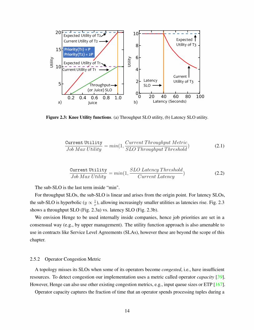
The maximum utility value is based on job priority. For example, in Fig. 2.3a, topology T2 hastwice the priority of T1, and thus has twice the maximum utility (20 vs. 10).

Given these requirments, Henge is able to allow a wide variety of shapes for its utility functionsincluding: linear, piece-wise linear, step function (allowed because utilities are monotonicallynon-increasing instead of monotonically decreasing), lognormal, etc. Utility functions do not needto be continuous. All in all, this offers users flexibility in shaping utility functions according toindividual needs.

The concrete utility functions used in our Henge implementation are knee functions, depictedin Fig. 2.3. A knee function has two pieces: a plateau beyond the SLO threshold, and a sub-SLOpart for when the job does not meet the threshold. Concretely, the achieved utility for jobs withthroughput and latency SLOs respectively, are:

13

Expected Utility of T1

Throughput (or Juice) SLO

Current Utility of T2

Current Utility of T1

Expected Utility of T2Expected Utility of T3

Latency SLO

Current Utility of T3

Priority(T1) = PPriority(T2) = 2P

a) b)

Figure 2.3: Knee Utility functions. (a) Throughput SLO utility, (b) Latency SLO utility.

Current Utility

Job Max Utility= min(1,

Current Throughput Metric

SLO Throughput Threshold) (2.1)

Current Utility

Job Max Utility= min(1,

SLO Latency Threshold

Current Latency) (2.2)

The sub-SLO is the last term inside “min".For throughput SLOs, the sub-SLO is linear and arises from the origin point. For latency SLOs,

the sub-SLO is hyperbolic (y ∝ 1x

), allowing increasingly smaller utilities as latencies rise. Fig. 2.3shows a throughput SLO (Fig. 2.3a) vs. latency SLO (Fig. 2.3b).

We envision Henge to be used internally inside companies, hence job priorities are set in aconsensual way (e.g., by upper management). The utility function approach is also amenable touse in contracts like Service Level Agreements (SLAs), however these are beyond the scope of thischapter.

2.5.2 Operator Congestion Metric

A topology misses its SLOs when some of its operators become congested, i.e., have insufficientresources. To detect congestion our implementation uses a metric called operator capacity [39].However, Henge can also use other existing congestion metrics, e.g., input queue sizes or ETP [167].

Operator capacity captures the fraction of time that an operator spends processing tuples during a

14

time unit. Its values lie in the range [0.0, 1.0]. If an executor’s capacity is near 1.0, then it is close tobeing congested.

Consider an executor E that runs several (parallel) tasks of a topology operator. Its capacity iscalculated as:

CapacityE =Executed TuplesE × Execute LatencyE

Unit T ime(2.3)

where Unit T ime is a time window. The numerator multiplies the number of tuples executed inthis window and their average execution latency to calculate the total time spent in executing thosetuples. The operator capacity is then the maximum capacity across all executors containing it.

Henge considers an operator to be congested if its capacity is above the threshold of 0.3. Thisincreases the pool of possibilities, as more operators become candidates for receiving resources(described next).

2.6 HENGE STATE MACHINE

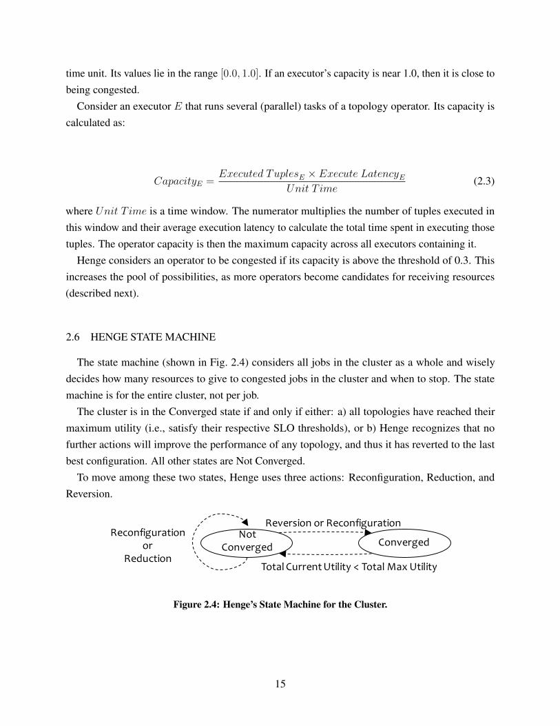
The state machine (shown in Fig. 2.4) considers all jobs in the cluster as a whole and wiselydecides how many resources to give to congested jobs in the cluster and when to stop. The statemachine is for the entire cluster, not per job.

The cluster is in the Converged state if and only if either: a) all topologies have reached theirmaximum utility (i.e., satisfy their respective SLO thresholds), or b) Henge recognizes that nofurther actions will improve the performance of any topology, and thus it has reverted to the lastbest configuration. All other states are Not Converged.

To move among these two states, Henge uses three actions: Reconfiguration, Reduction, andReversion.

Reconfiguration or

Reduction Converged

Total Current Utility < Total Max Utility

Reversion or ReconfigurationNot

Converged

Figure 2.4: Henge’s State Machine for the Cluster.

15

2.6.1 Reconfiguration

In the Not Converged state, a Reconfiguration gives resources to topologies missing their SLO.Reconfigurations occur in rounds which are periodic intervals (currently 10 s apart). In each round,Henge first sorts all topologies missing their SLOs, in descending order of their maximum utility,with ties broken by preferring lower current utility. It then picks the head of this sorted queue toallocate resources to.

This greedy strategy works best to maximize cluster utility.Within this selected topology, the intuition is to increase each congested operator’s resources by

an amount proportional to its respective congestion. Henge uses the capacity metric (Section 2.5.2,eq. 2.3) to discover all congested operators in this chosen topology, i.e., operator capacity > 0.3. Itallocates each congested operator an extra number of threads based on the following equation:

(Current Operator Capacity

Capacity Threshold− 1

)× 10 (2.4)

Henge deploys this configuration change to a single topology on the cluster, and waits for themeasured utilities to quiesce (this typically takes a minute or so in our configurations). No furtheractions are taken in the interim. It then measures the total cluster utility again, and if it improved,Henge continues its operations in further rounds, in the Not Converged State. If this total utilityreaches the maximum value (the sum of maximum utilities of all topologies), then Henge cautiouslycontinues monitoring the recently configured topologies for a while (4 subsequent rounds in oursetting). If they all stabilize, Henge moves the cluster to the Converged state.

A topology may improve only marginally after being given more resources in a reconfiguration,e.g., utility increases < 5%. In such a case, Henge retains the reconfiguration change but skips thisparticular topology in the near future rounds. This is because the topology may have plateaued interms of marginal benefit from getting more threads. Since the cluster is dynamic, this black-listingof a topology is not permanent but is allowed to expire after a while (1 hour in our settings), afterwhich the topology will again be a candidate for reconfiguration.

As reconfigurations are exploratory steps in the state space search, total system utility maydecrease after a step. Henge employs two actions called Reduction and Reversion to handle suchcases.

2.6.2 Reduction

If a Reconfiguration causes total system utility to drop, the next action is either a Reduction ora Reversion. Henge performs Reduction if and only if three conditions are true: (a) the cluster is

16

congested (we detail below what this means), (b) there is at least one SLO-satisfying topology, and(c) there is no past history of a Reduction action.

First, CPU load is defined as the number of processes that are running or runnable on a ma-chine [10]. A machine’s load should be ≤ number of available cores, ensuring maximum utilizationand no over-subscription. As a result, Henge considers a machine congested if its CPU load exceedsits number of cores. Henge considers a cluster congested when it has a majority of its machinescongested.

If a Reconfiguration drops utility and results in a congested cluster, Henge executes Reduction toreduce congestion. For all topologies meeting their SLOs, it finds all their un-congested operators(except spouts) and reduces their parallelism level by a large amount (80% in our settings). If thisresults in SLO misses, such topologies will be considered in future reconfiguration rounds. Tominimize intrusion, Henge limits Reduction to once per topology; this is reset if external factorschange (input rate, set of jobs, etc.). Akin to backoff mechanisms [92], massive reduction is theonly way to free up a lot of resources at once, so that future reconfigurations may have a positiveeffect. Reducing threads also decreases their context switching overhead.

Right after a reduction, if the next reconfiguration drops cluster utility again while keeping thecluster congested (measured using CPU load), Henge recognizes that performing another reductionwould be futile. This is a typical “lockout" case, and Henge resolves it by performing Reversion.

2.6.3 Reversion

If a Reconfiguration drops utility and a Reduction is not possible (meaning that at least one of theconditions (a)-(c) in Section 2.6.2 is not true), Henge performs Reversion.

Henge sorts through its history of Reconfigurations and picks the one that maximized systemutility. It moves the system back to this past configuration by resetting the resource allocations of alljobs to values in this past configuration and moves to the Converged state. Here, Henge essentiallyconcludes that it is impossible to further optimize cluster utility, given this workload. Hengemaintains this configuration until changes like further SLO violations occur, which necessitatereconfigurations.

If a large enough drop (> 5%) in utility occurs in this Converged state (e.g., due to new jobs,or input rate changes), Henge infers that as reconfigurations cannot be a cause of this drop, theworkload of topologies must have changed. As all past actions no longer apply to this change inbehavior, Henge forgets all history of past actions and moves to the Not Converged state. Thismeans that in future reversions, forgotten states will not be available. This reset allows Henge tostart its state space search afresh.

17

2.6.4 Discussion

Online vs. Offline State Space Search: Henge prefers an online state space search. In fact,our early attempt at designing Henge was to perform offline state space exploration (e.g., throughsimulated annealing), by measuring SLO metrics (latency, throughput) and using analytical modelsto predict their relation to resources allocated to the job.

Reconfiguration

Figure 2.5: Unpredictability in Modern Stream Processing Engines: Two runs of the same topology (on10 machines) being given the same extra computational resources (28 threads, i.e., executors) at 910 s, reactdifferently.

The offline approach turned out to be impractical. Analysis and prediction is complex and oftenturns out to be inaccurate for stream processing systems, which are very dynamic in nature. (Thisphenomenon has also been observed in other distributed scheduling domains, e.g., see [59,101,133].)We show an example in Fig. 2.5. The figure shows two runs of the same Storm job on 10 machines.In both runs we gave the job equal additional thread resources (28 threads) at t=910 s. Latencydrops to a lower value in run 2, but only stabilizes in run 1.

This is due to differing CPU resource consumptions across the runs. More generally, we findthat natural fluctuations occur commonly in an application’s throughput and latency; left to itselfan application’s performance changes and degrades gradually over time. We observed this for allour actions: reconfiguration, reduction, and reversion. Thus, we concluded that online state spaceexploration would be more practical.

Statefulness, Memory Bottlenecks: The common case among topologies is stateless operatorsthat are CPU-bound, and our exposition so far is thus focused. Nevertheless, Henge gracefullyhandles stateful operators and memory-pressured nodes (evaluated in Sections 2.9.3, 2.9.5).

Dynamically Added Jobs: Henge accepts new jobs deployed on the multi-tenant cluster as longas existing jobs are able to satisfy their SLOs. However, if the set of jobs the cluster starts with donot satisfy their SLOs, Henge employs admission control. A possible future direction may be thatif existing jobs on the cluster do not all satisfy their SLOs, Henge selects the maximum subset of

18

jobs from the existing and newly added jobs that can be deployed on the cluster while providingmaximum utility.

2.7 JUICE: DEFINITION AND ALGORITHM

This section describes the motivation for Juice and how it is calculated.As described in section 2.1, a throughput metric (for use in throughput SLOs) should be designed

in a way that is independent of input rate. Henge uses a new metric called juice. Juice defines whatfraction of the input data is being processed by the topology per unit time. It lies in the interval [0,1], and a value of 1.0 means all the input data that arrived in the last time unit has been processed.Thus, the user can set throughput requirements as a percentage of the input rate (Section 2.5.1), andHenge subsequently attempts to maintain this even as input rates change.

Any algorithm that calculates juice should satisfy three requirements:1. Code Independence: It should be independent of the operators’ code, and should be calculate-ableby only considering the number of tuples generated by operators.2. Rate Independence: It should abstract away throughput SLO requirements in a way that isindependent of absolute input rate.3. Topology Independence: It should be independent of the shape and structure of the topology.

Juice Intuition: Overall, juice is formulated to reflect the global processing efficiency of atopology. We define per-operator contribution to juice as the proportion of input passed in originallyfrom the source that the operator processed in a given time window. This reflects the impact of thatoperator and its upstream operators, on this input. The juice of a topology is then the normalizedsum of juice values of all its sinks.

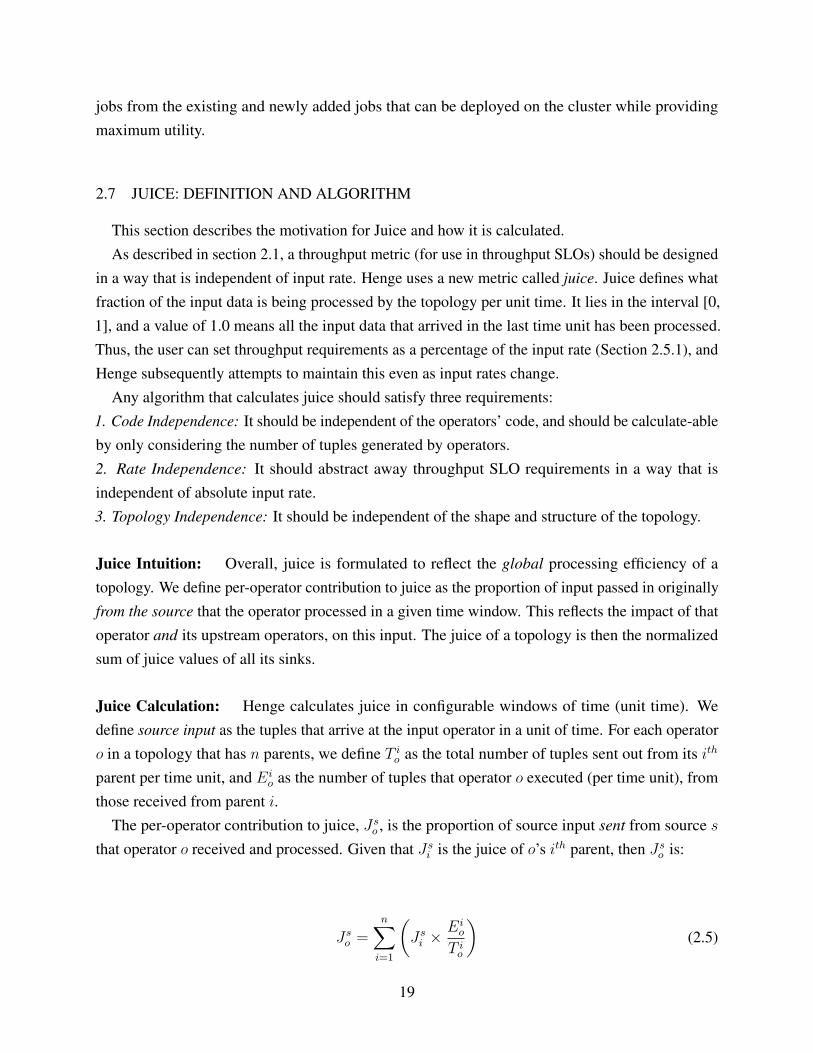
Juice Calculation: Henge calculates juice in configurable windows of time (unit time). Wedefine source input as the tuples that arrive at the input operator in a unit of time. For each operatoro in a topology that has n parents, we define T io as the total number of tuples sent out from its ith

parent per time unit, and Eio as the number of tuples that operator o executed (per time unit), from

those received from parent i.The per-operator contribution to juice, Jso , is the proportion of source input sent from source s

that operator o received and processed. Given that Jsi is the juice of o’s ith parent, then Jso is:

Jso =n∑i=1

(Jsi ×

Eio

T io

)(2.5)

19

A spout s has no parents, and its juice: Js = Es

Ts= 1.0 .

In eq. 2.5, the fraction Eio

T io

reflects the proportion of tuples an operator received from its parents,and processed successfully. If no tuples waiting in queues, this fraction is equal to 1.0. Bymultiplying this value with the parent’s juice we accumulate through the topology the effect of allupstream operators.

We make two important observations. In the term Eio

T io, it is critical to take the denominator as

the number of tuples sent by a parent rather than received at the operator. This allows juice: a) toaccount for data splitting at the parent (fork in the DAG), and b) to be reduced by tuples dropped bythe network. The numerator is the number of processed tuples rather than the number of outputtuples – this allows juice to generalize to operator types whose processing may drop tuples (e.g.,filter).

Given all operator juice values, a topology’s juice can be calculated by normalizing w.r.t. numberof sources:

∑Sinks si, Sources sj

(Jsjsi )

Total Number of Sources(2.6)

If no tuples are lost in the system, the numerator sum is equal to the number of sources. To ensurethat juice stays below 1.0, we normalize the sum with the number of sources.

Example 2.1: Consider Fig. 2.1 in Section 2.4. JsA = 1× 10K10K

= 1 and JsB = JsA × 8K16K

= 0.5.B has a TAB of 16K and not 8K, since B only receives half the tuples that were sent out by operatorA, and its per-operator juice should be in context of only this half (and not all source input).

The value of JsB = 0.5 indicates that B processed only half the tuples sent out by parent A. Thisoccurred as the parent’s output was split among children. (If (alternately) B and C were sinks (if Dwere absent from the topology), then their juice values would sum up to the topology’s juice.). D hastwo parents: B and C. C is only able to process 6K as it is congested. Thus, JsC = JsA× 6K

16K= 0.375.

TCD thus becomes 6K. Hence, JCD = 0.375× 6K6K

= 0.375. JBD is simply 0.5× 8K8K

= 0.5. We sumthe two and obtain JsD = 0.375 + 0.5 = 0.875. It is less than 1.0 as C was unable to process alltuples due to congestion.

Example 2.2 (Topology Juice with Split and Merge):In Fig. 2.6, we show how our approach generalizes to: a) multiple sources (spout 1 & 2), and b)

operators splitting output (E to B and F) and c) operators with multiple input streams (A and E toB). Bolt A has a juice value of 0.5 as it can only process half the tuples spout 1 sent it. Bolt D has a

20

Spout 1 Bolt A

Bolt E

Bolt B Bolt C

x2 as Bolt B duplicated all input

10000 tuples

10000 tuples

5000 tuples 10000

tuples

(5000 + 10000)x2 tuples

Congested Bolt A processes half of the tuples sent by the spout

Spout 2 Bolt D Bolt F

30000 tuples

10000 tuples

20000 tuples

20000 tuples

20000 tuples

Congested Bolt E processes half of tuples sent by D

Congested Bolt F only processes 8000 tuples sent by E

8000 tuples

JA = 0.5

JD = 1.0 JE =0.5

JB =0.75 JC =0.75

JF =0.2

Figure 2.6: Juice Calculation in a Split and Merge Topology.

juice value of 1.0. 50% of the tuples from D to E are unprocessed due to congestion at E. E passesits tuples on to B and F: both of them get half of the total tuples it sends out. Therefore, B has juiceof 0.25 from E and 0.5 from A (0.25+ 0.5 = 0.75). 20% of the tuples E sent F are unprocessed at Fas it is congested, so F has a juice value of 0.25× 0.8 = 0.2. C processes as many tuples as B sentit, so it has the same juice as B (0.75). The juice of the topology is the sum of the juices of the twosinks, normalized by the number of sources. Thus, the topology’s juice is 0.2+0.75

2= 0.475.

Some Observations: First, while our description used unit time, our implementation calculatesjuice using a sliding window of 1 minute, collecting data in sub-windows of length 10 s. Thisneeds only loose time synchronization across nodes (which may cause juice values to momentarilyexceed 1, but does not affect our logic). Second, eq. 2.6 treats all processed tuples equally–instead,a weighted sum could be used to capture the higher importance of some sinks (e.g., sinks feedinginto a dashboard). Third, processing guarantees (exactly, at least, at most once) are orthogonal tothe juice metric.

Our experiments use the non-acked version of Storm (at most once semantics), but Henge alsoworks with the acked version of Storm (at least once semantics). At least once semantics entailsthat if any tuples fail (i.e., they have to be reprocessed), we should proportionally reduce juice toonly reflect the amount of tuples acked. We do so in the following manner:

JFinal = Jso ×Total No. of Tuples Acked

Total No. of Tuples Sent by All Spouts(2.7)

This allows the juice metric to reflect only the tuples that have been processed and provide valueto the final result.

21

2.8 IMPLEMENTATION

This section describes how Henge is built and is integrated into Apache Storm [7].Henge involves 3800 lines of Java code. It is an implementation of the predefined IScheduler

interface. The scheduler runs as part of the Storm Nimbus daemon, and is invoked by Nimbusperiodically every 10 seconds. The developer can specify which scheduler to use in a configurationfile that is provided to Nimbus. Further changes were made to Storm Config, allowing users to settopology SLOs and utility functions while writing topologies.

Statistics Module

Decision Maker

New Schedule

Henge

Supervisor

Executor

Nimbus

Worker Processes

Figure 2.7: Henge Implementation: Architecture in Apache Storm.

Henge’s architecture is shown in Fig. 2.7. The Decision Maker implements the Henge statemachine of Section 2.6. The Statistics Module continuously calculates cluster and per-topologymetrics such as the number of tuples processed by each task of an operator per topology, theend-to-end latency of tuples, and the CPU load per node. This information is used to produce usefulmetrics such as juice and utility, which are passed to the Decision Maker. The Decision Maker runsthe state machine, and sends commands to Nimbus to implement actions.

The Statistics Module also tracks historical performance and configuration of topologies whenevera reconfiguration is performed by the Decision Maker, so that reversion can be performed.

2.9 EVALUATION

This section presents the evaluation of Henge with a variety of workloads, topologies, and SLOs.We answer the following necessary experimental questions:

22

1. Is juice truly independent of input rate, topology structure and operations? i.e., Is juice a goodabstraction for throughput?

2. How well does Henge perform as compared to finely-tuned manual configurations and vanillaStorm?

3. Is Henge able to maximize cluster utility for a variety of workloads e.g., diurnal workloads,spikes in input rate and production workloads?

4. Is Henge scalable and fault-tolerant?

Experimental Setup: By default, our experiments used the Emulab cluster [160], with machines(2.4 GHz, 12 GB RAM) running Ubuntu 12.04 LTS, connected via a 1 Gbps connection. Anothermachine runs Zookeeper [8] and Nimbus. Workers (Java processes running executors) are allottedto each of our 10 machines (we evaluate scalability later).

Bolt SinkBoltSpout

Bolt Sink

Bolt

Spout

Bolt

Linear Topology

Diamond Topology

Spout Bolt

Spout

Spout

Sink

Sink

Sink

Star Topology

Figure 2.8: Three Microbenchmark Topologies.

Transform

Sink

FilterSpout Join with database

FilterAggregate

Figure 2.9: PageLoad Topology from Yahoo!.

Topologies: For evaluation, we use both: a) micro-topologies that are possible sub-parts of largertopologies [167], shown in Fig. 2.8; and b) a production topology from Yahoo! Inc. [167]–thistopology is called “PageLoad" (Fig. 2.9). Operators are the ones that are most commonly usedin production: filtering, transformation, and aggregation. In each experimental run, we initially

23

allow topologies to run for 900 s without interference (to stabilize and to observe their performancewith vanilla Storm), and then enable Henge to take actions. All topology SLOs use the knee utilityfunction of Section 2.5.1. Hence, below we use “SLO” as a shorthand for the SLO threshold.

2.9.1 Juice as a Performance Indicator

Juice is an indicator of queue size: Fig. 2.10 shows the inverse correlation between topologyjuice and queue size at the most congested operator of a PageLoad topology. Queues buffer incomingdata for operator executors, and longer queues imply slower execution rate and higher latencies.Initially queue lengths are high and erratic–juice captures this by staying well below 1. At thereconfiguration point (910 s) the operator is given more executors, and juice converges to 1 as queuelengths fall, stabilizing by 1000 s.

Reconfig-uration

Reconfig-uration

a) b)

Que

ue S

ize

Juic

e

Figure 2.10: Juice vs. Queue Size: Inverse Relationship.

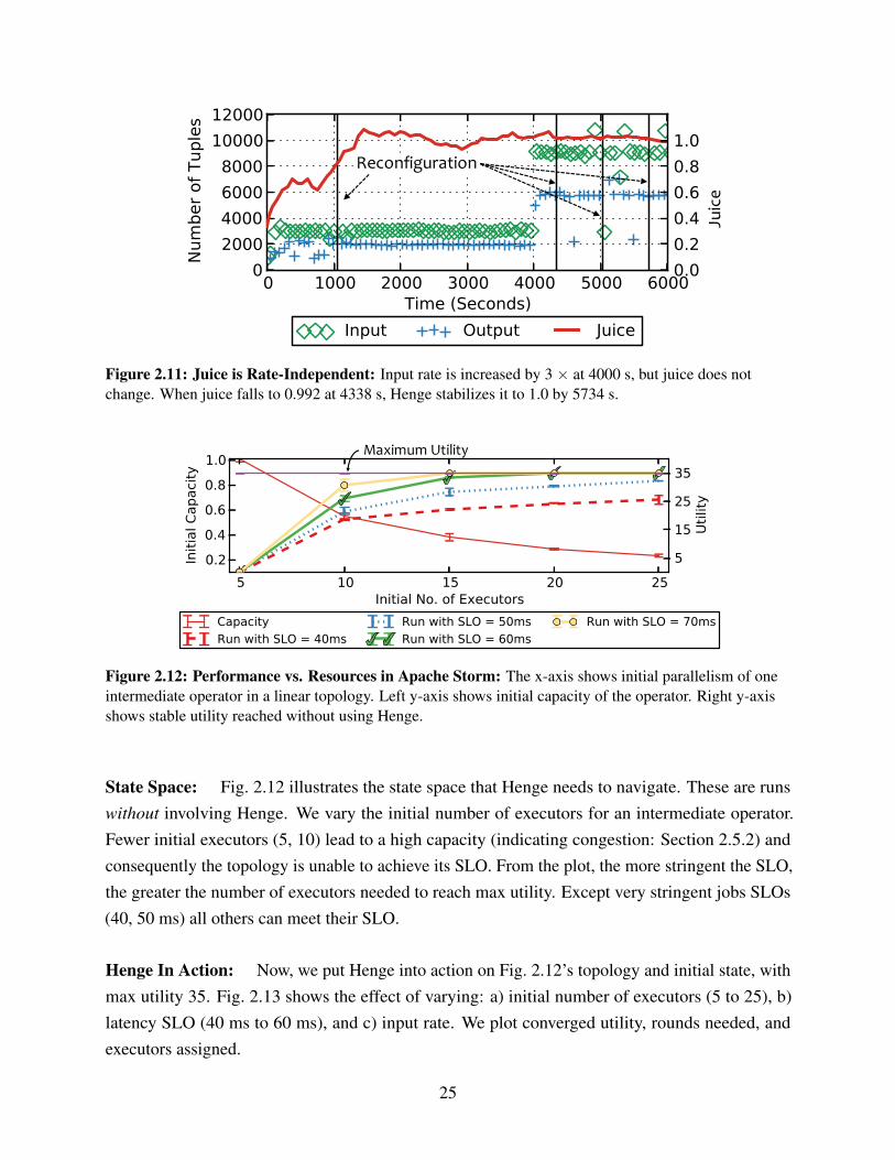
Juice is independent of operations and input rate: In Fig. 2.11, we run 5 PageLoad topologieson one cluster, and show data for one of them. Initially juice stabilizes to around 1.0, near t=1000 s(values above 1 are due to synchronization errors, but they don’t affect our logic). PageLoad filterstuples, thus output rate is < input rate–however, juice is 1.0 as it shows that all input tuples arebeing processed.

Then at 4000 s, we triple the input rate to all tenant topologies. Notice that juice stays 1.0. Dueto natural fluctuations, at 4338 s, PageLoad’s juice drops to 0.992. This triggers reconfigurations(vertical lines) from Henge, stabilizing the system by 5734 s, maximizing cluster utility.

2.9.2 Henge Policy and Scheduling

Impact of Initial Configuration:

24

Reconfiguration

Juice

Figure 2.11: Juice is Rate-Independent: Input rate is increased by 3 × at 4000 s, but juice does notchange. When juice falls to 0.992 at 4338 s, Henge stabilizes it to 1.0 by 5734 s.

Maximum Utility

Figure 2.12: Performance vs. Resources in Apache Storm: The x-axis shows initial parallelism of oneintermediate operator in a linear topology. Left y-axis shows initial capacity of the operator. Right y-axisshows stable utility reached without using Henge.

State Space: Fig. 2.12 illustrates the state space that Henge needs to navigate. These are runswithout involving Henge. We vary the initial number of executors for an intermediate operator.Fewer initial executors (5, 10) lead to a high capacity (indicating congestion: Section 2.5.2) andconsequently the topology is unable to achieve its SLO. From the plot, the more stringent the SLO,the greater the number of executors needed to reach max utility. Except very stringent jobs SLOs(40, 50 ms) all others can meet their SLO.

Henge In Action: Now, we put Henge into action on Fig. 2.12’s topology and initial state, withmax utility 35. Fig. 2.13 shows the effect of varying: a) initial number of executors (5 to 25), b)latency SLO (40 ms to 60 ms), and c) input rate. We plot converged utility, rounds needed, andexecutors assigned.

25

Late

ncy

SLO

= 4

0ms

a)

Late

ncy

SLO

= 5

0ms

b)

Util

ity (%

)U

tility

(%)

Late

ncy

SLO

= 6

0ms

Late

ncy

SLO

= 7

0ms

Util

ity (%

)U

tility

(%)

Figure 2.13: Effect of Henge on Figure 2.12’s initial configurations: SLOs become more stringent frombottom to top. We also explore a 2 × higher input rate. a) Left y-axis shows final parallelism level Hengeassigned to each operator. Right y-axis shows number of rounds required to reach said parallelism level. b)Utility values achieved before and after Henge.

We observe that generally, Henge gives more resources to topologies with more stringent SLOsand higher input rates. For instance, for a congested operator initially assigned 10 executors in a 70ms SLO topology, Henge reconfigures it to have an average of 18 executors, all in a single round.On the other hand, for a stricter 60 ms SLO it assigns 21 executors in two rounds. When we doublethe input rate of these two topologies, the former is assigned 36 executors in two rounds and thelatter is assigned 44, in 5 rounds.

Henge convergence is fast. In Fig. 2.13a, convergence occurs within 2 rounds for a topology witha 60 ms SLO. Convergence time increases for stringent SLOs and higher input rates. With the 2 ×higher input rate convergence time is 12 rounds for stringent SLOs of 50 ms, vs. 7 rounds for 60 ms.

26

Henge always reaches max utility (Fig. 2.13b) unless the SLO is unachievable (40, 50 ms SLOs).Since Henge aims to be minimally invasive, we do not explore operator migration (but we coulduse them orthogonally [129, 130, 136]). With an SLO of 40 ms, Henge actually performs fewerreconfigurations and allocates less resources than with a laxer SLO of 50 ms. This is because the 40ms topology gets black-listed earlier than the 50 ms topology ( Section 2.6.3: recall this occurs ifutility improves < 5% in a round).

Overall, by black-listing topologies with overly stringent SLOs and satisfying other topologies,Henge meets its goal of preventing resource hogging (Section 2.3).

T9 T8 T8 T7 T6 T5 T4T6 T3 T3 T2T1 T1

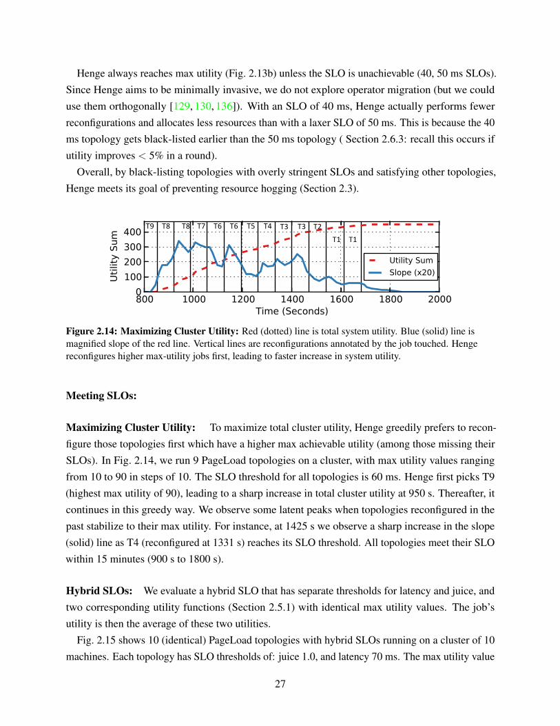
Figure 2.14: Maximizing Cluster Utility: Red (dotted) line is total system utility. Blue (solid) line ismagnified slope of the red line. Vertical lines are reconfigurations annotated by the job touched. Hengereconfigures higher max-utility jobs first, leading to faster increase in system utility.

Meeting SLOs:

Maximizing Cluster Utility: To maximize total cluster utility, Henge greedily prefers to recon-figure those topologies first which have a higher max achievable utility (among those missing theirSLOs). In Fig. 2.14, we run 9 PageLoad topologies on a cluster, with max utility values rangingfrom 10 to 90 in steps of 10. The SLO threshold for all topologies is 60 ms. Henge first picks T9(highest max utility of 90), leading to a sharp increase in total cluster utility at 950 s. Thereafter, itcontinues in this greedy way. We observe some latent peaks when topologies reconfigured in thepast stabilize to their max utility. For instance, at 1425 s we observe a sharp increase in the slope(solid) line as T4 (reconfigured at 1331 s) reaches its SLO threshold. All topologies meet their SLOwithin 15 minutes (900 s to 1800 s).

Hybrid SLOs: We evaluate a hybrid SLO that has separate thresholds for latency and juice, andtwo corresponding utility functions (Section 2.5.1) with identical max utility values. The job’sutility is then the average of these two utilities.

Fig. 2.15 shows 10 (identical) PageLoad topologies with hybrid SLOs running on a cluster of 10machines. Each topology has SLO thresholds of: juice 1.0, and latency 70 ms. The max utility value

27

Maximum Utility T2 T5 T10 T3 T8 T4 T7 T1 T6 T9 T9 T9

Util

ity S

um

Figure 2.15: Hybrid SLOs: Henge Reconfiguration.

of each topology is 35. Henge only takes about 13 minutes (t=920 s to t=1710 s) to reconfigure alltopologies successfully to meet their SLOs. 9 out of 10 topologies required a single reconfiguration,and one (T9) required 3 reconfigurations.

Tail Latencies: Henge can also admit SLOs expressed as tail latencies (e.g., 95th percentile, or99th percentile). Utility functions are then expressed in terms of tail latency and the state machineremains unchanged. Fig.2.16 depicts a case where five PageLoad topologies are unable to meettheir SLO. All are latency-sensitive with utilities of 35, and threshold of 80 ms. Henge performsone reconfiguration for each topology allowing all topologies to meet their SLO. The figure alsoshows the 99th percentile tail latency values. for the scenario. As every reconfiguration removescongestion from operators, we can see that the tail latencies improve as well.

Handling Dynamic Workloads:

A. Spikes in Workload: Fig. 2.17 shows the effect of a workload spike in Henge. Two differentPageLoad topologies A and B are subjected to input spikes. B’s workload spikes by 2 ×, startingfrom 3600 s. The spike lasts until 7200 s when A’s spike (also 2 ×) begins. Each topology’s SLO is80 ms with max utility is 35. Fig. 2.17 shows that: i) output rates keep up for both topologies bothduring and after the spikes, and ii) the utility stays maxed-out during the spikes. In effect, Hengecompletely hides the effect of the input rate spike from the user.

B. Diurnal Workloads: Diurnal workloads are common for stream processing in production, e.g.,in e-commerce websites [70] and social media [128]. We generated a diurnal workload based on thedistribution of the SDSC-HTTP [36] and EPA-HTTP traces [13], injecting them into PageLoadtopologies.

5 topologies are run with the SDSC-HTTP trace and concurrently, 5 other topologies are run with

28

Time(seconds)

Utility

T3T2 T1

T2T1

T3

T5T4

T3T2T1T5T4

(a) The latencies of the topologies in ms as reconfigurationoccurs.

Time(seconds)

Utility

T3T2 T1

T2T1

T3

T5T4

T3T2T1T5T4

(b) The latencies of the topologies at the 99th percentile

Time(seconds)

Utility

T3T2 T1

T2T1

T3

T5T4

T3T2T1T5T4

(c) Individual utilities of the topologies.

Figure 2.16: Tail Latencies: 5 PageLoad topologies run on a cluster.

the EPA-HTTP trace. All 10 topologies have max-utility=10 (max achievable cluster utility=350),and a latency SLO of 60 ms.

Fig. 2.18 shows the results of running 48 hours of the trace (each hour mapped to 10 min intervals).In Fig. 2.18a workloads increase from hour 7 of the day, reach their peak by hour 131

3, and then start

to fall. Within the first half of Day 1, Henge successfully reconfigures all 10 topologies, reaching byhour 15 a cluster utility that is 89% of the max.

29

Figure 2.17: Spikes in Workload: Left y-axis shows total cluster utility (max possible is 35× 2 = 70).Right y-axis shows the variation in workload as time progresses.

(a)

(b)

(d)

(c)

Figure 2.18: Diurnal Workload: a) Input and output rates over time, for two different diurnal workloads.b) Utility of a topology (reconfigured by Henge at runtime) with the EPA workload, c) Utility of a topology(reconfigured by Henge at runtime) with the SDSC workload, d) CDF of SLO satisfaction for Henge, defaultStorm, and manually configured. Henge adapts during the first cycle and fewer reconfigurations are requiredthereafter.

30

Fig. 2.18b shows a topology running the EPA workload and Fig. 2.18c a topology running theSDSC workload. Observe how Henge reconfigurations from hour 8 to 16 adapt to the fast changingworkload. This also results in fewer SLO violations during the second peak (hours 32 to 40). Thus,even without adding resources, Henge tackles diurnal workloads. Fig. 2.18d shows the CDF of SLOsatisfation for the three systems. Default Storm performs poorly, giving 0.0006% SLO satisfactionat the median, and 30.9% at the 90th percentile. (This means that 90% of the time, default Stormprovided a total of at most 30.9% of the cluster’s max achievable utility.) Henge yields 74.9% ,99.1%, and 100% SLO satisfaction at the 15th, 50th, and 90th percentiles respectively.

Henge is also better than manual configurations. We manually configured all topologies to meettheir SLOs at median load.

These provide 66.5%, 99.8% and 100% SLO satisfaction at the 15th, 50th and 90th percentilesrespectively. Henge is better than manual configurations from the 15th to 45th percentile, andcomparable from then onwards. Henge has an average of 88.12% SLO satisfaction rate, whereasdefault Storm and manually configured topologies provide an average of 4.56% and 87.77%respectively. Thus, Henge provides 19.3 × better SLO satisfaction than default Storm, and performsbetter than manual configuration.

Production Workloads: We configured the sizes of 5 PageLoad topologies based on data from aYahoo! Storm production cluster and Twitter datasets [51], shown in Table 2.3. We use 20 nodeseach with 14 worker processes. For each topology, we inject an input rate proportional to its numberof workers. T1-T4 run sentiment analysis on Twitter workloads from 2011 [51]. T5 processes logsat a constant rate. Each topology has a latency SLO threshold of 60 ms and max utility value of 35.

Job Workload Workers TasksT1 Analysis (Egypt Unrest) 234 1729T2 Analysis (London Riots) 31 459T3 Analysis (Tsunami in Japan) 8 100T4 Analysis (Hurricane Irene) 2 34T5 Processing Topology 1 18

Table 2.3: Job and Workload Distributions in Experiments: Derived from Yahoo! production clusters,using Twitter Datatsets for T1-T4. (Experiments in Figure 2.19.)

This is an extremely constrained cluster where not all SLOs can be met. Yet, Henge maximizescluster utility. Fig. 2.19a shows the CDF of the fraction of time each topology provided a givenutility (including the initial 900 s where Henge is held back). T5 shows the most improvement (atthe 5th percentile, it has 100% SLO satisfaction), whereas T4 shows the worst performance (at the

31

(a) CDF of the fraction of total time tenant topologies provide a given SLO satisfaction. Max utility for each topologyis 35.

Reverts last action

ReductionT1 T4 T1 T4

(b) Reconfiguration at 32111 s causes a drop in total system utility. Henge reverts the configuration of all tenants to thatof 32042 s. Vertical lines show Henge actions for particular jobs.

Figure 2.19: Henge on Production Workloads.

median, its utility is 24, which is 68.57% of 35). The median SLO satisfaction for T1-T3 rangesfrom 27.0 to 32.3 (77.3% and 92.2% respectively).

Reversion: Fig. 2.19b depicts Henge’s reversion. At 31710 s, the system utility drops due tonatural system fluctuations. This forces Henge to perform reconfigurations for two topologies(T1, T4). Since system utility continues to drop, Henge is forced to reduce a topology (T5, whichsatisfies its SLO before and after reduction. As utility improves at 32042 s, Henge proceeds toreconfigure other topologies. However, the last reconfiguration causes another drop in utility (at32150 s). Henge reverts to the configuration that had the highest utility (at 32090 s). After thispoint, total cluster utility stabilizes at 120 (68.6% of max utility). Thus, even under scenarios whereHenge is unable to reach the max system utility it behaves gracefully, does not thrash, and convergesquickly.

Reacting to Natural Fluctuations: Natural fluctuations occur in the cluster due to load variationthat arises from interfering processes, disk IO, page swaps, etc. Fig. 2.20 shows such a scenario.We run 8 PageLoad topologies, 7 of which have an SLO of 70 ms, and the 8th SLO is 10 ms. Hengeresolves congestion initially and stabilizes the cluster by 1000 s. At 21800 s, CPU load increasessharply due to OS behaviors (beyond Henge’s control). Seeing the significant drop in cluster utility,Henge reduces two of the topologies (from among those meeting their SLOs). This allows othertopologies to recover within 20 minutes (by 23000 s). Henge converges the system to the same totalutility as before the CPU spike.

32

Load on machinesduring marked time

a)

b)

Reconfigurations Reductions

Maximum Utility

Util

ity S

um

Figure 2.20: Handling CPU Load Spikes: a) Total cluster utility. b) Average CPU load on machines in theCPU spike interval.

2.9.3 Stateful Topologies

Job Type Avg. Reconfig. Average ConvergenceRounds (Stdev) Time (Stdev)

Stateful 5.5 (0.58) 1358.7355 (58.1s)Stateless 4 (0.82) 1134.2235 (210.5s)

Table 2.4: Stateful Topologies: Convergence Rounds and Times for a cluster with Stateful and StatelessTopologies.

Henge handles stateful topologies gracefully, alongside stateless ones. We ran four WordCounttopologies with identical workload and configuration as T2 in Table 2.3. Two of these topologiesperiodically checkpoint state to Redis (making them stateful) and have 240 ms latency SLOs. Theother two topologies do not persist state in an external store and have lower SLOs of 60 ms. Initially,none of the four meet their SLOs. Table 2.4 shows results after convergence. Stateful topologiestake 1.5 extra reconfigurations to converge to their SLO, and only 19.8% more reconfigurationtime. This difference is due to external state checkpointing and recovery mechanisms, orthogonal toHenge.

2.9.4 Scalability and Fault-tolerance

We vary number of jobs and nodes, and inject failures.

33

Scalability:

Increasing the Number of Topologies: Fig. 2.21 stresses Henge by overloading the cluster withtopologies over time. We start with a cluster of 5 PageLoad topologies, each with a latency SLO of70 ms, and max utility value of 35. Every 2 hours, we add 20 more PageLoad topologies.

Maximum Utility

No.

of

(a) Green (dotted) line is average job utility. Blue (solid) line is number of job on cluster. Vertical black lines arereconfigurations.

5, 20, 5 20, 25Number of Topologies Residing on the Cluster (New, Pre-Existing)

0 20, 45Aver

age

Reco

nfig

urat

ions

(b) Average number of reconfigurations that must take place when new topologies are added tothe cluster.

Figure 2.21: Scalability w.r.t. No. of Topologies: Cluster has 5 tenants. 20 tenants are added every 2hours until the 8 hour mark.

Henge stabilizes better when there are more topologies. In the first 2 hours, Fig. 2.21a showsthat the average utility of the topologies is below the max, because Henge has less state space tomaneuver with fewer topologies. 20 new tenant topologies at the 2 hour mark cause a large drop inaverage utility but also open up the state space more–Henge quickly improves system utility to themax value. At the 4 hour and 6 hour marks, more topologies arrive. Henge stabilizes to max utilityin both cases.

Topologies arriving at the 8 hour mark cause contention. In Fig. 2.21a, the average system utilitydrops not only due to the performance of the new tenants, but also because the pre-existing tenants

34

are hurt. Henge converges both types of topologies, requiring fewer reconfiguration rounds for thepre-existing topologies (Fig. 2.21b).

Increasing Cluster Size: In Fig. 2.22 we run 40 topologies on clusters ranging from 10 to 40nodes. The machines have two 2.4 GHz 64-bit 8-core processors, 64 GB RAM, and a 10 Gbpsnetwork. 20 topologies are PageLoad with latency SLOs of 80 ms and max utility 35. Among therest, 8 are diamond topologies, 6 are star topologies and 6 are linear topologies, with juice SLOs of1.0 and max utility 5.

b)a)

c)

b)a)

c)

(a) CDF of jobs according to fraction of SLO thresholds reached.

b)a)

c)

CDF

b)a)

c)

(b) CDF of convergence time.b)a)

c)

Average

Reconfigurations

(c) No. of reconfigurations until convergence.

Figure 2.22: Scalability w.r.t. No. of Machines. 40 jobs run on cluster sizes increasing from 10 to 40 nodes.

From Fig. 2.22a, Henge is able to provide SLO satisfaction for 40% of the tenants even in anoverloaded cluster of 10 nodes. As expected, in large clusters Henge has more room to maneuver

35

and meets more SLOs. This is because CPUs saturate slower in larger clusters. In an overloadedcluster of 10 nodes, topologies at the 5th percentile are able to achieve only 0.3% of their max utility.On the other hand, in clusters with 20, 30, and 40 machines, 5th percentile SLO satisfactions arehigher: 56.4%, 74.0% and 94.5% respectively.

Fig. 2.22b shows the time taken for topologies to converge to their highest utility. Interestingly,while the 10 node cluster has a longer tail than 20 or 30 nodes, it converges faster at the median(537.2 seconds). Topologies at the tail of both the 10 and 40 node clusters take a longer time toconverge. This is because in the 10 node cluster, greater reconfiguration is required per topologyas there is more resource contention (see Fig. 2.22c). At 40 nodes, collecting cluster informationfrom Nimbus daemons leads to a bottleneck. This can be alleviated by decentralized data gathering(beyond our scope).

Fig. 2.22c shows that the number of reconfigurations needed to converge is at most 2 × higherwhen resources are limited and does not otherwise vary with cluster size. Overall, Henge’sperformance generally improves with cluster size, and overheads are scale-independent.

Fault Tolerance: Henge reacts gracefully to failures. In Fig. 2.23, we run 9 topologies each with70 ms SLO and 35 max utility. We introduce a failure at the worst possible time: in the midst ofHenge’s reconfiguration operations, at 1020 s. This severs communication between Henge and allthe worker nodes; and Henge’s Statistics module is unable to obtain fresh information about jobs.We observe that Henge reacts conservatively by avoiding reconfiguration in the absence of data. At1380 s, when communication is restored, Henge collects performance data for the next 5 minutes(until 1680 s) and then proceeds with reconfigurations as usual, meeting all SLOs.

Maximum Utility

Reconfigurations

Failure Recovery

Reconfigurations

Util

ity S

um

Figure 2.23: Fault-tolerance: Failure occurs at t=1020s, and recovers at t=1380 s. Henge makes no wrongdecisions due to the failure, and immediately converges to the max system utility after recovery.

36

Reconfigurations

Figure 2.24: Memory Utilization: 8 jobs with joins and 30 s tuple retention.

2.9.5 Memory Utilization

Fig. 2.24 shows a Henge cluster with 8 memory-intensive topologies. Each topology has a maxutility value of 50 and a latency SLO of a 100 ms. These topologies have join operations, andtuples are retained for 30 s, creating memory pressure at some cluster nodes. As the figure shows,Henge reconfigures memory-bound topologies quickly to reach total max utility of 400 by 2444s,and keeps average memory usage below 36%. Critically, the memory utilization (blue dotted line)plateaus in the converged state, showing that Henge is able to handle memory-bound topologiesgracefully.

2.10 RELATED WORK

This section presents relevant related work in the areas of elastic stream processing, cluterscheduling, multi-tenant resource management and SLA/SLO satisfaction in other areas.

2.10.1 Elastic Stream Processing Systems

Traditional query-based stream processing systems such as Aurora [45] and Borealis [46] provideload-balancing [149] but not first-class multi-tenant elasticity. Modern general-purpose stream pro-cessing systems [4–7,35,47,112,127] do not natively handle adaptive elasticity. Ongoing work [12]on Spark Streaming [168] allows scaling but does not apply to resource-limited multi-tenant clusters.SEEP [63] describes a single approach for scaling out stateful operators and recovering from failuresbased on check-pointing but does not discuss scale-in or resource distribution in the presence ofmultiple tenants. Similarly, TimeStream [139] describes resilient substitution as a single method forfault recovery and resource reconfiguration without addressing multi-tenancy.

Resource-aware elasticity in stream processing [57, 64, 76, 106, 108, 135, 145] assumes infinite

37

resources that the tenant can scale out to. [52, 78, 93, 114, 119, 146, 163] propose resourceprovisioning but not multi-tenancy. Some works have focused on balancing load [129, 130],optimal operator placement [84, 105, 136] and scaling out strategies [85, 86] in stream processingsystems. These approaches can be used in complement with Henge in various ways. [84–86] lookat single-job elasticity, but not multi-tenancy.

Themis’ [107] SIC metric is similar to juice, but the two systems have different goals. Themismeasures the weight of each tuple to find those that can be dropped to reduce load, while Hengeuses juice to support SLOs.

Dhalion [75] describes a system that provides the capabilities of self-regulation to stream pro-cessing systems, namely Heron. It only supports throughput SLOs and uses triggers such asbackpressure to detect whether a single topology is failing and then carries out dynamic resourceprovisioning to resolve the issue. However, backpressure is a very coarse-grained measure of SLOsatisfaction – by the time backpressure is triggered, a latency SLO in place by the user may alreadybe violated. In addition, backpressure completely stops tuples flowing in the topology, meaning thatresources are consumed for a topology even though it is doing no work. Henge simply uses SLOviolations as a trigger for corrective measures and is able to satisfy both latency and throughputSLOs in a multi-tenant environment.

2.10.2 Multi-tenant Resource Management Systems

Resource schedulers like YARN [156] and Mesos [90] can be run under stream processingsystems, and manually tuned [65].

Since the job internals are not exposed to the scheduler (jobs run on containers) it is impossibleto make fine-grained decisions for stream processing jobs in an automated fashion.

2.10.3 Cluster Scheduling

Some systems propose scheduling solutions to address resource fairness and SLO achieve-ment [71, 72, 80, 121, 141, 147]. VM-based scaling approaches [109] do not map directly andefficiently to expressive frameworks like stream processing systems. Among multi-tenant streamprocessing systems, Chronostream [164] achieves elasticity through migration across nodes. It doesnot support SLOs.

2.10.4 Video Stream Processing Systems

Henge is not built for video stream processing systems specifically, where techniques are neededto reduce the high cost of vision processing. For example, some existing schedulers for video stream

38

processing focus on the characteristics of the video stream to reduce the amount of resources usedper job as much as possible. VideoStorm is a system that processes video analytics queries on livevideo streams [172]. VideoStorm’s offline profiler generates a query resource-quality profile, whileits online scheduler allocates resources to queries to maximize performance on quality and lag, asopposed to the commonly used fair sharing of resources in clusters.

Applications use video data in varying ways. One challenge is applying deep neural networksto video data, which requires massive computational resources. Chameleon [99] is a controllerthat dynamically picks the best configurations for existing NN-based video analytics pipelines.Chameleon utilizes the fact that underlying characteristics of video streams (e.g., the velocity andsize) that affect the best configuration have enough temporal and spatial correlation to allow thesearch cost of finding the best configuration to be amortized over time and across multiple videofeeds.

Deployments of video streaming have also been explored in wide-area scenarios, where it faces thechallenges of variable WAN bandwidth. AWStream [170] is a stream processing system that achieveslow latency and high accuracy in this setting through three insights: (i) it integrates applicationadaptation as a first-class abstraction in the stream processing model (ii) with a combination ofoffline and online profiling, it automatically learns an accurate profile that models accuracy andbandwidth trade-off, and (iii) at runtime, it adjusts the application data rate to match the availablebandwidth while maximizing the achievable accuracy.

2.10.5 SLAs/SLOs in Other Areas

SLAs/SLOs have been explored in other areas. Pileus [152] is a geo-distributed storage systemthat supports multi-level SLA requirements dealing with latency and consistency. Tuba [55] buildson Pileus and performs reconfiguration to adapt to changing workloads. SPANStore [165] is ageo-replicated storage service that automates trading off cost vs. latency, while being consistent andfault-tolerant.

E-store [148] re-distributes hot and cold data chunks across nodes in a cluster if load exceeds athreshold. Cake [159] supports latency and throughput SLOs in multi-tenant storage settings.

To the best of our knowledge, Henge is the first work that combines elastic resource managementfor stream processing systems in a multi-tenant environment.

2.11 CONCLUSION

We presented Henge, a system for intent-driven (SLO-based) multi-tenant stream processing.Henge provides SLO satisfaction for topologies (jobs) with latency and/or throughput requirements.

39

To make throughput SLOs independent of input rate and topology structure, Henge uses a newrelative throughput metric called juice. In a cluster, when jobs miss their SLO, Henge uses threekinds of actions (reconfiguration, reversion or reduction) to improve the sum utility achieved byall jobs throughout the cluster. Our experiments with real Yahoo! topologies and Twitter datasetshave shown that in multi-tenant settings with a mix of SLOs, Henge: i) converges quickly to maxsystem utility when resources suffice; ii) converges quickly to a high system utility when the clusteris constrained; iii) gracefully handles dynamic workloads, both abrupt (spikes, natural fluctuations)and gradual (diurnal patterns, Twitter datasets); iv) scales gracefully with cluster size and numberof jobs; and v) is failure tolerant.

40

Chapter 3: Caladrius: A Performance Modelling Service for Distributed Stream ProcessingSystems

Real-time processing has become increasingly important in recent years and has led to thedevelopment of a multitude of stream processing systems. Given the varying job workloads thatcharacterize stream processing, these systems need to be tuned and adjusted to match incomingtraffic.

Current scaling systems adopt a series of trials to approach a job’s expected performance due to alack of performance modeling tools. In this chapter, we show that general traffic trends in most jobslend themselves well to prediction. Based on this premise, we built a system called Caladrius thatforecasts future traffic load of a stream processing job and predicts the job’s processing performanceafter scaling. Experimental results show that Caladrius is able to estimate a job’s throughputperformance and CPU load under a given scaling configuration.

3.1 INTRODUCTION

Many use cases of the deluge of data that is pouring into organizations today require real-timeprocessing. Common examples of such use cases include internal monitoring jobs that allowengineers to react to service failures before they cascade, jobs that process ad-click rates, andservices that identify trending conversations in social networks, etc.

Many distributed stream processing systems (DSPSs) have been developed to cater to this risingdemand, that provide high-throughput and low-latency processing of streaming data. For instance,Twitter uses Apache Heron [112], LinkedIn relies on Apache Samza [6] and others use ApacheFlink [62]. Usually, DSPSs run stream processing jobs (or topologies) as a directed acyclic graph(DAG) of operators that perform user-defined computation on incoming data (also called tuples).

These systems are generally well-equipped to self-tune their configuration parameters and achieveself-stabilization against unexpected load variations. For example, Dhalion [75] allows DSPSsto monitor their jobs, recognize symptoms of failures and implement necessary solutions. Mostcommonly, Dhalion scales out job operators to stabilize their performance.

In addition to Dhalion, there are many examples from the research community of attemptsto create automatic scaling systems for DSPSs. These examples usually consist of schedulerswhose goal is to minimize certain criteria, such as the network distance between operators thatcommunicate large tuples or very high volumes of tuples, or to ensure that no worker nodes areoverloaded by operators that require a lot of processing resources [78, 84, 85]. While the new jobdeployments these schedulers produce may be improvements over the original ones, none of thesesystems assess whether these deployments are actually capable of meeting a performance target

41

or service level objective (SLO). A job’s “deployment” refers to it’s packing plan, defined as amapping of operator instances to runnable containers (described in Section 3.2.)

This lack of performance prediction and evaluation is problematic: it requires the user (or anautomated system) to run the new job deployment, wait for it to stabilize and for normal operationto resume, possibly wait for high traffic to arrive and then analyze the metrics to see if the requiredperformance has been met. Depending on the complexity of the job and the traffic profile, it maytake weeks for a production job to be scaled to the correct configuration.

A performance modelling system that can provide the following benefits is necessary to handlethese challenges:

Faster tuning iterations during deployment Auto-scaling systems use performance metrics fromphysical deployments to make scaling decisions that allow jobs to meet their performancegoals. Performance modelling systems that are able to evaluate a proposed deployment’sperformance can eliminate the need for physical job executions, thus making each iterationfaster. Of course, any modelling system is subject to errors so some re-deployment may berequired, however the frequency and thus, the length of the tuning process can be significantlyreduced.

Improved scheduler selection A modelling system would allow several different proposed jobdeployments to be assessed in parallel. This means that schedulers optimized for differentcriteria can be compared simultaneously, which helps achieve the best performance withoutprior knowledge of these different schedulers.

Enabling preemptive scaling A modelling system can accept predictions of future workloads (e.g.defined by tuple arrival rate) and trigger preemptive scaling if it finds that a future workloadwould overwhelm the current job deployment.

Caladrius1 is a performance modelling service for DSPSs.The aim of this service is to predict potential job performance under varying traffic loads

and/or deployments, thus 1) reducing the time required to tune a topology’s configuration for agiven incoming traffic load. This significantly shortens the loop of ‘plan –> deploy –> stabilize–> analyze’ that is currently required to tune a topology; 2) enabling preemptive scaling beforedisruptive workloads arrive. Caladrius can be easily extended to provide other analyses of topologylayouts and performance.

Caladrius provides a framework to analyze, model and predict various aspects of DSPSs (such asApache Heron [112] and Storm [154]) and focuses on two key areas:

1This is the Roman name for the legend of the healing bird that takes sickness into itself

42

• Traffic: The prediction of the incoming workload of a stream processing topology. Caladriusprovides interfaces for accessing metrics databases and methods that analyze traffic enteringa topology and predict future traffic levels.

• System Performance: The prediction of a topology’s performance under a given traffic loadand deployment plan. This can be broken down into two scenarios:

? Under varying traffic load: The prediction of how a topology will perform underdifferent or future traffic levels if it keeps its current deployment.

? Using a different deployment plan: The prediction of how a topology will perform undercurrent traffic levels if its layout is changed.

1. Motivated by challenges that users face, we introduce the notion of DSPSs modeling to enablefast job tuning and preemptive scaling, and discuss its properties.

2. We present Caladrius, the first performance modelling and evaluation tool for DSPSs (Sec-tion 3.3, 3.4). Caladrius has a modular and extensible architecture and has been implementedon top of Apache Heron.

3. We validate the proposed models and present one use case for performance assessment andprediction for stream processing topologies (Section 3.5).

We discuss related work in Section 3.6. Finally, we draw conclusions in Section 3.7. In the nextsection, we start by presenting job scaling and scheduling background (Section 3.2).

3.2 BACKGROUND

This section presents a brief overview of DSPSs as well as related concepts and terminologies,particularly those belonging to Apache Heron [112], on which Caladrius is built. Terms areformatted as italics in this section and the rest of the chapter aligns to the term definitions here.

3.2.1 Topology Components

A stream processing topology can be logically represented as a DAG of components or operators.A component is a logical processing unit, defined by the developer, that applies user-definedfunctions on a stream of input data, called tuples. The edges between components representthe dataflow between the computational units. Source components are called spouts in Heronterminology, and they pull tuples into the topology, typically from sources such as pub-sub systemslike Kafka [111]. Tuples are processed by downstream components called bolts.

43

Spout

Count

a)Logicaltopology

Components

b)Packingplan

MetricsManager

StreamManager

Container1 Instances

c)Atuple’spaththroughthetopology

Spout

Spout

[“Soitgoes…”] [“Soitgoes…”]

ShuffleGrouping

FieldsGrouping

Spout Count

Count

Splitter

MetricsManager

StreamManager

Container 2

Spout Count

Count

Splitter

StreamManager

StreamManager

Splitter

Splitter

StreamManager

StreamManager

Count

Count

Count

Count[“goes”]

[“So”]

[“it”]

[“So”][“it”][“goes”]…

Splitter

Figure 3.1: Sentence-Word-Count Topology a) A logical DAG of the topology as the developer writes it. b)A physical representation of the topology when it is run. c) A possible path an input might take through thetopology.

We define three kinds of throughputs: 1) source throughput, the throughput that the source pub-sub system provides, waiting to be processed by the topology; 2) spout throughput, the throughputprocessed by spouts which allows data to enter the topology; 3) output throughput, the sum outputthroughput of all sink bolts i.e. the job’s final output throughput. We use the terms throughput andtraffic interchangeably in this chapter.

A job can be saturated due to limited resources where its processing throughput cannot catchup with the pub-sub system’s source throughput. Then, data accumulates in the source pub-subsystem waiting to be fetched. For example, we can have a topology where Kafka generates source

throughput = 5 million tuples in a minute, the topology’s spouts try their best to read from Kafkawith spout throughput = 3 million tuples, and the whole topology generates output throughput = 10million tuples. In this example, Kafka accumulates 5− 3 = 2 million tuples.

3.2.2 Topology Instances

The developer specifies how many parallel instances there should be for each component: this iscalled the component’s parallelism level. In other words, instances perform the same processinglogic on different input data. All instances of the same component are of same resource configuration.The developer also specifies how tuples from each component’s instances should be partitionedamongst the downstream component’s instances. These partitioning methods are called grouping.The most common grouping is called shuffle grouping, where data can be partitioned randomlyacross downstream instances. Field grouping chooses the downstream instance based on the hash of

44

the data in a tuple whereas all grouping replicates the entire stream to all the downstream instances.

3.2.3 Implementation of DSPSs

We consider long-running stream processing topologies with a continuous operator model. Atopology master (tmaster) is responsible for managing the topology throughout its existence andprovides a single point of contact for discovering the status of the topology. Each topology is run ona set of containers using an external scheduler, e.g. Twitter uses Aurora [45] for this purpose. Eachcontainer consists of

• one or more Heron-Instances (instances),

• a metrics manager and

• a stream manager (stmgr),

each of which is run as a dedicated Java process. The metrics manager is responsible for routingmetrics to the topology master or a central metrics service in data center, while the stream manageris responsible for routing tuples between running instances. An instance processes streaming dataone tuple at a time (thus emulating the continuous operator model) and forwards the tuples to thenext components in the topology, via the stream manager. Systems that follow such a model includeApache Heron [112], Samza [6], Flink [62] and Storm [154].

3.2.4 A Topology Example

We present a sample topology in Figure 3.1. Figure 3.1a) shows the logical representation of thetopology, where tuples are ingested into the topology from the spout, and passed onto Splitter boltsthat split sentences in the tuples to words. The resulting tuples are then passed onto the Counterbolts that count the occurrence of each unique word.

Figure 3.1b) shows how the topology may look when launched on a physical cluster. Theparallelism level of the spout and the Splitter bolt are both 2 and the parallelism level of the Counterbolt is 4. The topology is run in two containers, each of which contains a stream manager forinter-instance communication. This representation of a topology is called its packing plan.

Figure 3.1c) shows a possible path a tuple could take in a topology. Though only one path isshown here, there are 16 possible paths for the job, given the parallelism levels of the components.Stream managers are used for passing tuples between two instances. If two instances on the samecontainer need to communicate, data will only pass through the local container’s stream manager.On the other hand, if the instances run on different containers, the sender’s output tuples will first go

45

Caladrius APIConfig and Class Loader Logging

Topology Throughput

Prediction Model

Back Pressure Evaluation Model

Topology Performance Model Interface

Prophet Traffic Model

Statistic Summary Traffic Model

Traffic Model Interface

TinkerPopCuckoo

Metrics Interface

Heron MetricsCache

Topology Metadata Interface

Heron Tracker

Graph Interface

API T

ier

Mod

el T

ier

Mod

el H

elpe

r Tie

rTraffic Modelling Request Performance Modelling Request

Modelling Results (JSON)

Figure 3.2: Caladrius System Overview.

to its local stream manager, who will then send them to the stream manager on the remote container.The receiving stream manager will be in charge of passing those tuples onto the local receivinginstance. Note that this does not increase the number of possible paths in the topology.

3.3 SYSTEM ARCHITECTURE

This section presents a brief overview of Caladrius’ architecture, particularly with respect to itsinterface with Apache Heron [112]. Caladrius consists of three tiers—the API tier, the model tierand the shared model helper tier—as shown in Figure 3.2. It is deployed as a web service that caneasily be launched in a container, and is accessible to developers through a RESTful API providedby the API tier.

3.3.1 API Tier

The API tier faces users who would like to use Caladrius to predict future traffic levels or perfor-mance of a topology. It is essentially a web server translating and routing user HTTP requests tocorresponding interfaces. Caladrius exposes several RESTful endpoints to allow clients to querythe various modelling systems it provides. Currently, Caladrius provides topology performance(throughput, back pressure etc.) and traffic (incoming workload) modelling services. Besidesperforming HTTP request handling, the API tier is also a web container that hosts implementa-

46

tions of the aforementioned models and fulfills system-wide common shared logistics includingconfiguration management and logging, etc.

It is important to consider that a call to the topology modelling endpoints may incur a wait (upto several seconds, depending on the modelling logic). Therefore, it is prudent to let the API beasynchronous, allowing the client to continue with other operations while the modelling is beingprocessed. Additionally, an asynchronous API allows the server side calculation pipelines to runconcurrently with ease.

A response for a call to a RESTful endpoint hosted by the API tier is a JSON formatted string.This string contains the results of modelling and prediction. The type of results listed can vary bymodel implementation. By default, the endpoint will run all model implementations defined in theconfiguration and concatenate the results into a single JSON response.

3.4 MODELS: SOURCE TRAFFIC FORECAST & TOPOLOGY PERFORMANCEPREDICTION

As discussed in the Section 3.3, Caladrius is a modular and extensible system that allows users toimplement their own models to meet their performance estimation requirements. Here, we presenta typical use case of Caladrius to evaluate one of the four golden system performance signals –“traffic”, and extensively discuss the implementation of the “source traffic forecast” and “topologyperformance prediction” models on top of Heron. Our models can be applied to other DSPSs aslong as they employ topology-based stream flow and backpressure-based rate control mechanisms.

3.4.1 Source Traffic Forecast

Caladrius must be able to forecast a job’s source traffic rate. This is necessary for finding out thetopology’s performance in the near future. We measure the job’s source traffic rate as a timeseriesfor the purposes of forecast. The timeseries consists of tuple counts waiting to be processed bya topology per minute per minute. We assume that no bottlenecks exist between the spouts andthe external source, such that spout throughput is the same as source throughput. Intuitively, thisremains true unless the topology experiences backpressure where spout throughput falls belowsource throughput.

Time series forecasting is a complex field of research and many methods for predicting futuretrends from past data exist. A simple statistics summary such as mean or median of the last givenperiod of data points may be sufficient for a reasonable forecast of a random timeseries.

However, we find that a large percentage of topologies in the field depict strong seasonality. Asimple statistical model is not able to predict such strongly seasonal traffic rates. To deal with

47

seasonality, we use more sophisticated modelling techniques. Specifically, we use Facebook’sProphet, a framework for generalized timeseries modelling [150]. It is based on an additive modelwhere non-linear trends are fit with periodic (yearly, weekly, daily, etc.) seasonality. It is robust tomissing data, shifts in the trend, and large outliers [150].

Caladrius allows users to pass the model a length of historic data and specify whether a singleProphet model should be used for tuple streams entering each spout as a whole, or separate modelsshould be created for tuple streams entering each spout instance. A spout can have many instances,depending on its parallelism level. The latter method is slower but more accurate. The user alsospecifies the time in future we should forecast the traffic rate. The model then produces varioussummary statistics e.g. mean and median, for the predicted input rate at the future instance, basedon historic data.

3.4.2 Topology Performance Prediction

The previous subsection described how we forecast source traffic levels for a topology. Thisincoming data is passed to downstream components that process it to find results. To make anaccurate performance estimation about how the topology will perform at a particular traffic level,we must study the impact of the traffic level on each instance’s performance.

Modelling Single Instance Throughput

Based on our production experience with Heron, we have the following topology performanceobservations and we summarize them into assumptions used for topology performance modelling.

Neither Heron-Stmgr nor the network is a bottleneck. The Heron-Stmgr behaves like a routerinside the container. It routes all the traffic for all instances in the container. As the Heron-Stmgr is hidden from the end user’s perspective, it is hard for the end users to reason aboutit if it forms a bottleneck. Thus, almost all users in the field allocate a large number ofcontainers to their jobs. This means that there are a few instances per container, ensuringthat the Heron-Stmgr is never a bottleneck despite variable input rates. Thus, we assume thatthe throughput bottleneck is not Heron-Stmgr and backpressure is triggered only when theprocessing speed of the instances is less than their input throughput.

Backpressure is either 0 or 1; there is no intermediate state. In Heron, backpressure is triggeredby default if the amount of data pending for processing at one instance exceeds 100Mb (highwater mark). Backpressure is resolved if the amount of pending data is below 50Mb (lowwater mark). Given Twitter’s traffic load, tiny traffic variance can push 50Mb of data to

48

Outputthroughput

Sourcethroughput

Non-saturation (Non-backpressure)interval

Saturation (backpressure)interval

Saturation throughput(ST)

Saturation point(SP)

Linearrelation

Figure 3.3: Topology performance observation in Heron production experience.

instances. This means that although the instances just finished processing data and reducedthe amount of pending data below the lower water mark, just enough data is pushed to themthat the high water mark is exceeded again. This forces the instance to continue to be inbackpressure unnecessarily.

Heron adopts a metric named “backpressure time” to measure how many seconds (in therange from 0 to 60) in a minute when the topology is in backpressure state. Based on theabove, “backpressure time” is either close to 60 or is 0, rather than being evenly distributed.Thus, we can approximate the topology’s backpressure state to be either 0 or 1.

Based on the assumptions above, we draw the output throughput performance of an instance witha single upstream instance and single downstream instance in Figure 3.3. We observe the followingfeatures:

Saturation Point (SP) of source throughput: If input traffic rates exceed a threshold, a job’sinstances can trigger backpressure. We call this the saturation point (SP) of the instances.When input traffic rises beyond the SP, instances will always face backpressure.

Saturation Throughput (ST) of output throughput: After the input traffic rate exceeds the SP,an instance’s output throughput reaches and stays at a maximum value, called its saturationthroughput (ST). This is because even though input rates are rising, the instance is alreadypushed to its maximum processing rate.

49

Linear relation (α) of output and source throughputs: When backpressure is not present andthe instance is not saturated, its processing throughput is the same as its input throughput.A linear relation between output throughput and input throughput exists, and its slope (α)represents the amplifier coefficient of the instance which is determined by its linear processinglogic (together with grouping types if multiple downstream instances exist). Intuitively,ST = αSP .

It should be noted that for a large amount of tuples, such as those belonging to Twitter’s trafficload, the variation of processing times per tuple are normalized, rendering the processingspeed steady and content agnostic.

Given these observations, we express the output throughput Ti of a single-input single-outputinstance i against source throughput tλ, which is most commonly seen in production, as follows:

Ti(tλ) =

{αitλ : tλ < SPi

STi : tλ ≥ SPi(3.1)

or simplyTi(tλ) = min(αitλ, STi). (3.2)

The output throughput of instances with multiple (m) input streams can be calculated as:

Ti(tλ) =m∑λ=1

min(αitλ, STi) (3.3)

This approach assumes that input and output streams have a linear relationship, which workswell in practice for most topologies. When an instance has only one input, Equation 3.3 reduces toEquation 3.2.

Moreover, if there are n outputs, Equation 3.3 becomes:

Ti(tλ) =n∑j=1

Tj(tλ) (3.4)

Tj(tλ) =m∑λ=1

min(αjtλ, STj), j ∈ [1, 2, ..., n] (3.5)

where Tj(tλ), αj and STj represent the output throughput, the amplifier coefficient and the saturationthroughput of the jth output stream respectively. αj is determined by both the instance’s processinglogic and the type of tuple grouping.

50

Modelling Single Component Throughput

Adding the throughput of all instances of a component gives the component’s throughput. Let’sconsider a single-input single-output component c first; the multi-input multi-output component’sthroughput can be derived from the single-input single-output component in the same way as donefor instances in section 3.4.2. Given the component’s parallelism level p, let the input throughput ofeach instance of the component be tλ(1), tλ(2), ..., tλ(p). The component’s input throughput is then:

tλ =

p∑i=1

tλ(i). (3.6)

The component output throughput is:

Tc(p, tλ) =

p∑i=1

Ti(tλ(i)). (3.7)

Since a component’s instances have the same code, they perform the same function T (). However,the input throughput tλ(i) to each instance i may not be same due to the upstream grouping type,specified by the user. Here we discuss the impact of the most commonly used grouping types ofshuffle (round robin or load balanced) and fields (key) grouping.

Shuffle Grouped Connections Shuffle grouped connections between components share outputtuples evenly across all downstream instances, leading to

tλ(1) = tλ(2) = ... = tλ(p) =tλp. (3.8)

This means that the routing probability from a source instance to a downstream instance is alwayssimply 1/p where p is the number of downstream instances, irrespective of the input traffic’s contentand changes in it over time.

The component output throughput is:

Tc(p, tλ) = pTi(tλp). (3.9)

Particularly, when p = 1, the component has a single instance and Equation 3.9 reduces toTc = Ti. When p > 1, Equation 3.9 shows that Tc becomes Ti times the number of instances (p).

Consider a component running for a while with seasonally varying input rates. We observeseveral data points of the same parallelism p and a range tλ ∈ (η1, η2) of input. Thus, we can drawa line Tc(tλ) similar to Figure 3.3 as long as SP exists in the range (η1, η2). This line corresponds to

51

the particular parallelism p. Given this line, we can draw another line of a new parallelism p′ = γp

by scaling the existing line by γ.

Fields Grouped Connections Fields grouping chooses downstream instances based on the hashof the data in the tuple and thus can depend on the content of the data. However, we observed thatthe data set bias towards certain downstream instances remains unchanged in a long-time window,or the bias changes slowly. This bias can be measured by periodically auditing traffic. Thus, weassume that the input traffic bias remains unchanged over time in the following discussions. Wediscuss two changes in a job’s execution: 1) varying input traffic load and 2) scaling a component toa new parallelism.

• Varying source traffic load while keeping parallelism constant:

By observing the input throughput at a particular parallelism level of an operator, we canidentify whether the data flow is biased towards a subset of instances belonging to downstreamcomponents. This allows us to predict the amount of data each downstream instance willreceive if the input rate changes.

Let the new overall input throughput be t′λ = βtλ. With the steady data set bias assumption,traffic distribution is measured along time and is distributed across all p parallel instances ofthe operator.

Thus, we have:

t′λ = βtλ =

p∑i=1

βtλ(i). (3.10)

We can calculate the component output throughput under a different input traffic load (Equa-tion 3.11). We observe that the output throughput of each instance is proportional to theoriginal one by β when its new input traffic load falls into the linear interval, and reaches thesaturation throughput otherwise.

Tc(p, t′λ) = Tc(p, βtλ)

=

p∑i=1

Ti(βtλ(i))

=

p∑i=1

min (βTi(tλ(i)), STi) (3.11)

• Varying parallelism while keeping input traffic load constant:

Changing parallelism can effect how tuples are distributed among instances when usingfields grouping. This complicates the calculation of the routing probability for fields grouped

52

connections under a different parallelism. The routing probability is a function of the data inthe tuple stream and their relative frequency; thus, the proportion of tuples that go to eachdownstream instance depends entirely on the nature of the data contained in the tuples.

Fields grouping chooses an instance to send data to by moding the hash value of the tuple bythe number of parallel instances. As the hash result depends on the tuple data, the result isunpredictable. However, we found in some cases that the data set distribution is uniform orload-balanced in a large data sample set. Under this circumstance, the component behavesas Equation 3.9. A potential solution for a biased data set is that a user can implement theirown Heron-customized-key-grouping to make the traffic distribution predictable and plug thecorresponding model into Caladrius.

Modelling Topology Throughput

A topology is a DAG, which can contain a critical path – the path which limits the wholetopology’s throughput. Once the model for each component is built, the throughput performance onthe critical path can be evaluated. We assume that there are N components on the critical path, andthe input traffic coming through the spouts is t0, which can be either the measured actual throughoutor forecasted source throughput in Section 3.4.1. The user specifies the parallelism configurationfor each component to be {p1, p2, ..., pN}. The output throughput of the critical path (tcp) can becalculated by chaining Equation 3.7:

tcp = Tc(N)(pN , Tc(N−1)(...Tc(2)(p2, Tc(1)︸ ︷︷ ︸N

(p1, t0)))...) (3.12)

Once we have tcp, we can trace backwards and find the saturation point of the topology:

t′0 = T−1c(1)(T−1c(2)(...T

−1c(N−1)(T

−1c(N)︸ ︷︷ ︸

N

(tcp)))...) (3.13)

Moreover, we can identify if there is or will potentially be backpressure by comparing t0 and t′0:

riskbackpressure =

{low : t′0 < t0

high : t′0 ∼ t0(3.14)

We can also locate the component or instance with high backpressure risk while creating the chainin Equation 3.12. For some topologies, the critical path cannot be identified easily. Under thissituation, multiple critical path candidates can be considered and predicted at the same time. Thecritical path selection problem is out of the scope of this chapter.

53

3.5 EXPERIMENTAL EVALUATION

As we depend on the Prophet library for the source traffic forecast modeling, the performanceevaluation of Caladrius’ traffic prediction will not be discussed here. We focus on the evaluationof the topology performance prediction model and its integration into Caladrius as an end-to-endsystem. The evaluation is conducted in two main parts.

1. First, we evaluate the output throughput. We validate our observation and assumptions for thesingle instance in Section 3.5.2, and the models for the single component in Section 3.5.3and the critical path in Section 3.5.4. DSPSs usually provide scaling commands to update theparallelism of their components. For example, Heron provides the ‘heron update [parallelism]’command to update a component’s parallelism in the topology DAG. Although users havetools to scale jobs, it is hard to predict changes in performance after running the commands.Some existing systems, such as Dhalion, use several rounds of ‘heron update [parallelism]’ toconverge Heron topologies to the users’ expected throughput service level objective (SLO) ina time-consuming process.

Conversely, Caladrius can predict the expected throughput given new component parallelismlevels, which gives users useful insights on how to tune their jobs. This can be done byexecuting the command ‘heron update –dry-run [parallelism]’. It should be noted that withthe ‘–dry-run’ parameter, the new packing plan and the expected throughput is calculatedwithout requiring job deployment, thus significantly reducing iteration time.

2. Besides throughput, we also conduct CPU load estimation for updated parallelism levels inSection 3.5.5. The CPU load primarily relates to the processing throughput, which makes itsprediction feasible once we have a throughput prediction.

3.5.1 Experimental Setup

Previous work on DSPSs [75] used a typical 3-stage Word Count topology to evaluate the systemsunder consideration. In our work, we use the same topology, shown in Figure 2.1. In this topology,the spout reads a line in from the fictional work “The Great Gatsby” as a sentence and emits it. Thespouts distribute the sentences to the bolts (Splitter) belonging to the second stage of the topologyusing shuffle grouping. The Splitter bolts split the sentences into words that subsequently forwardthe words to the third stage bolts (Counter) using fields grouping. Finally, the Counter bolts countthe number of times each word has been encountered. Unless mentioned otherwise, the spout’sparallelism in each experiment is set to 8.

As there is no external data source in the experiments, the spout output traffic matches the

54

configured throughput if there is no backpressure triggered by the job instances, and their throughputis reduced if backpressure is triggered.

We run the topology on Aurora, a shared cluster with Linux “cgroups” isolation. The topologyresource allocation is calculated by Heron’s round-robin packing algorithm – 1 CPU core and 2GBRAM per instance, with disk not involved in the evaluation. Note that the evaluation topologywas constructed primarily for this empirical evaluation, and should not be construed as being therepresentative topology for Heron workloads at Twitter.

We use throughput (defined in Section 3.2) as the evaluation metric in our experiments. We notethat the throughput of a spout is defined as the number of tuples emitted by the spout per minute.The throughput of a bolt is defined as the number of tuples generated by the bolt per minute.

We tune the Word Count topology to perform in ways that we expect in production settings i.e.,there are no out-of-memory (OOM) crashes, or any other failure due to resource starvation duringscheduling or long repetitive GC cycles. The experiments were allowed to run for several hours toattain steady state before measurements were retrieved.

3.5.2 Single Instance Model Validation

To validate the single instance model in Figure 3.3, we set the Splitter component’s parallelism to1. The topology was configured to have an input traffic rate of from 1 to 20 million tuples per minutewith an additional step of 1 million tuples per minute. Meanwhile, the Counter parallelism is set to3 to prevent it from being the bottleneck. We collect the Splitter processed-count and emit-countmetrics as they represent the instance’s input and output throughput. The observation was repeatedfor 10 times, and the throughput with 0.9 confidence is drawn in Figure 3.4.

There are two series of measurements of the Splitter instance in Figure 3.4. One is the inputthroughput and the other is output throughput. The x-axis is the spout’s output rate, and the y-axisshows the two series value in million tuples per minute. We can see the two series increase untilaround the point of 11 million spout emit-throughput, which is the SP. After SP, both series tend tobe steady, among which the output throughput is the ST.

Figure 3.5 shows the ratio of output over input throughput, which is between 7.63 and 7.64 - avery tight window, thus it can be roughly treated as a constant value. The slope actually representson average, the number of words in a sentence.

Moreover, we noticed the slope slightly fluctuates in the non-saturation interval, which is possiblydue to competition for resources in instances. An instance contains two threads: a gateway threadthat exchanges data with the Heron-Stmgr and a worker thread that performs the actual processingof the instance. When the input rate increases, the burden on the instance gateway thread andcommunication queues increases, which results in less resources allocated to the processing thread.

55

0

10

20

30

40

50

60

70

80

90

0 5 10 15 20Outputthroughput(milliontuplesperm

inute)

Source throughput (milliontuplesperminute)

sourceavgsource0.9lowsource0.9highoutputavgoutput0.9lowoutput0.9high

Figure 3.4: Instance output and input throughput vs. topology input rate.

However, the performance degradation in the processing thread is small and transient.Time spent in backpressure is presented in Figure 3.6. It can be observed that backpressure occurs

when the spout throughput reaches around 11 million (SP). The time spend in backpressure risessteeply from 0 to around 60000 milliseconds (1 minute) after it is triggered.

From the observation above, we note that to uniquely identify the curve for a given instance,we need at least two data points: one falls in the non-saturation interval and one in the saturationinterval. We can get these points from two experiments: one without and one with backpressure.

3.5.3 Single Component Model Validation and Component Throughput Prediction

When we observe jobs in a data center, source traffic varies along time and may have the samethroughput at multiple times. This means that we can observe multiple instances of a particularsource traffic rate. In the experiments, we emulate multiple observations of the same input rate byrestarting the topology and observing its throughput multiple times.

To validate the single component model, we follow the previous single instance evaluation: wefocus on the Splitter component and start with a parallelism of 3 as in Figure 3.7.

We can see that the throughput lines of a component have similar shape to those of the instancesshown in Figure 3.4, but scaled according to the parallelism. The topology input rate ranges from 2to 68 million tuples per minute, and the SP is around 30 million. The piecewise linear regressionlines are also marked as dash lines, and the output over input ratio can be calculated to be 7.638

56

7.6

7.61

7.62

7.63

7.64

7.65

7.66

7.67

7.68

0 5 10 15 20

Output/sourcera

tio

Source throughput (milliontuplesperminute)

Figure 3.5: Instance output/input throughput ratio vs. topology input rate.

(210.239/27.526), which is consistent with the result in Figure 3.5.Based on the observation of the Splitter bolt with a parallelism of 3, we can predict its throughput

with another parallelism level. Given the discussions of Equation 3.9, we plotted the predictionsof throughput with parallelism 2 and 4, as dashed lines for both input and output, in Figure 3.7.The predicted input and output ST with a parallelism of 2 is around 18 million and 140 millionrespectively, while those for parallelism of 4 are 36 million and 280 million.

To evaluate the prediction, we deployed the topology with Splitter component parallelism to be2 and 4, and measured throughput as shown in the Figure 3.8. In the non-backpressure interval,the predicted curves strictly match the measured ones. The ST prediction error, which is definedas the difference between the corresponding predicted and observed regression lines over theobserved regression line of output throughput (|STprediction−STobservation|/STobservation), is around(140− 136)/136 = 2.9% for parallelism of 2 and (287− 280)/280 = 2.5% for parallelism 4.

We can see that the ST predictions of parallelism 2 and 4 match well with the measured ones,with acceptable small variations.

3.5.4 Critical Path Model Validation and Topology Throughput Prediction

For the example job in Figure 2.1, the critical path is the only path going through the threecomponents. In the previous experiments, we have built the model for the Splitter component. Wedid the same for the Counter component and show its model in Figure 3.9. Moreover, we observed

57

0

10000

20000

30000

40000

50000

60000

70000

0 5 10 15 20

Backpressuretime(m

s)

Sourcethroughput (milliontuplesperminute)

Figure 3.6: Instance backpressure time vs. topology input rate.

the test dataset is unbiased fortunately, thus we use Equation 3.9 for the sink bolt.Now we have all the three component models on the critical path, and we can predict the critical

path throughput by applying Equation 3.12. We choose the parallelisms in Figure 2.1. The predictedsink bolt’s output rate is shown in Figure 3.10. Meanwhile, we deployed a topology with the sameparallelism in our data center, and measured its sink bolt output rate, shown in Figure 3.10. Thefigure shows the observation matches the prediction with an error of (139− 135)/139 = 2.8%.

3.5.5 Use Case: Predict CPU load

Input rate significantly impacts an instance’s resource usage such as CPU and memory. Thetasks assigned to a job’s instances can be categorized as CPU-intensive and memory-intensive tasks,whose CPU and memory load can be predicted.

Two factors are worth considering while performing our micro-benchmarks: 1) The saturationstate i.e., whether a component triggers backpressure. When the component triggers backpressure,its CPU or memory load is supposed to be at the maximum possible level as the processingthroughput of its instances also reaches their maximum points. 2) The resource limits of containersthat run the instances (especially in terms of memory). Instances may exceed the container memorylimit when their input throughput rises to high levels, which is rare in a well-tuned production jobbut can still happen.

In this section, we choose the CPU load of instances as an example. We observed that the CPU

58

0

50

100

150

200

250

300

0 10 20 30 40 50 60 70

Outputthroughput(milliontuplesperm

inute)

Sourcethroughput (milliontuplesperminute)

sourceavg source0.9low

source0.9high output avg

output 0.9low output 0.9high

sourceregression output regression

p=2sourceprediction p=2output prediction

p=4sourceprediction p=4output prediction

Figure 3.7: Component throughput measurements of the Splitter bolt for parallelism 3 and predictions forparallelism 2 and 4.

usage is linear to the output throughput per instance. Once we have the observation of several datapoints of <CPU load, output rates, source rates>, we can prepare two intermediate results:

• We can depict the throughput model <CPU load, output rates, source rates>, as we did in theprevious evaluations.

• We can then use the model <CPU load, output rates, source rates> to calculate the linear ratioor the slope ψ = CPU load

output throughput.

Given the target input throughput, we use our model <CPU load, output rates, source rates>,to find the estimated output rates. We then amplify the output rates by ψ to get the CPU load

59

0

50

100

150

200

250

300

350

0 10 20 30 40 50 60 70

Outputthroughput(milliontuplesperm

inute)

Sourcethroughput (milliontuplesperminute)

p=2sourceavgp=2source0.9lowp=2source0.9highp=2output avgp=2output 0.9lowp=2output 0.9highp=4sourceavgp=4source0.9lowp=4source0.9highp=4output avgp=4output 0.9lowp=4output 0.9highp=2sourcepredictionp=2output predictionp=4sourcepredictionp=4output prediction

Figure 3.8: Validation on throughput prediction for parallelisms 2 and 4 for the Splitter bolt.

estimation.We set the parallelism level of the Splitter bolt to 3 and observe the CPU load of its instances

in Figure 3.11. The CPU load is collected from the Heron JVM native metric ‘__jvm-process-cpu-load’, which presents the “recent cpu usage” for the Heron instance’s JVM process. The predictedCPU load regression line are shown in the same figure as dashed lines for parallelisms 2 and 4 forthe Splitter bolt.

Additionally, we configured the source throughput to the corresponding throughput and measuredits CPU load for parallelisms 2 and 4 for the Splitter bolt. Figure 3.12 shows the measured CPU loadvs. the predicted values. The prediction error is (2.399− 2.284)/2.399 = 4.8% for a parallelism

60

0

50

100

150

200

250

0 100 200 300 400 500Outputthroughput(m

illiontuplesper

minute)

Source throughput (milliontuplesperminute)

p=3avg p=30.9lowp=30.9high regressionp=4prediction

Figure 3.9: Component Counter throughput: observation and prediction.

of 2 and (4.568− 4.435)/4.435 = 3% for a parallelism of 4, which is higher than the throughputprediction error. This is because error has accumulated for the chained prediction steps.

3.6 RELATED WORK

3.6.1 Performance Prediction

Traffic prediction is used for performance improvements in several areas. For instance, theability to predict video traffic in video streaming can significantly improve the effectiveness ofnumerous management tasks, including dynamic bandwidth allocation and congestion control.Authors of [118] use a neural network-based approach for video traffic prediction and show that theprediction performance and robustness of neural network predictors can be significantly improvedthrough multiresolution learning.

Similarly, several predictors exist in the area of communication networks such as ARIMA,FARIMA, ANN and wavelet-based predictors [74]. Such prediction methods are used for efficientbandwidth allocation (e.g., in [120]) to facilitate statistical multiplexing among the local networktraffic.

However, the work done on traffic prediction in DSPSs is limited. For instance, authors of [166]perform traffic monitoring and re-compute scheduling plans in an online manner to redistribute

61

0

20

40

60

80

100

120

140

160

180

200

0 10 20 30 40 50 60 70

Outputthroughput(milliontuplesperm

inute)

Sourcethroughput (milliontuplesperminute)

criticalpathpredictioncriticalpathavgcriticalpath0.9lowcriticalpath0.9high

Figure 3.10: Topology predicted throughput and measured throughput.

0

0.5

1

1.5

2

2.5

3

3.5

4

4.5

5

0 10 20 30 40 50 60 70

CPUload(cores)

Sourcethroughput (milliontuplesperminute)

cpuloadavg cpuload0.9lowcpuload0.9high regressionlinep=2prediction p=4prediction

Figure 3.11: CPU load observation and prediction.

Storm job workers to minimize internode traffic.Authors of [117] proposed a predictive scheduling framework to enable fast, distributed stream

processing, which features topology-aware modeling for performance prediction and predictivescheduling. They presented a topology-aware method to accurately predict the average tuple

62

0

1

2

3

4

5

6

0 10 20 30 40 50 60 70

CPUload(cores)

Sourcethroughput (milliontuplesperminute)

p=2cpuload0.9low p=2cpuload0.9highp=2cpuloadavg p=2predictionp=4prediction p=4cpuloadavgp=4cpuload0.9low p=4cpuload0.9high

Figure 3.12: Validation on CPU load prediction.

processing time of an application for a given scheduling solution, according to the topology of theapplication graph and runtime statistics. They then present an effective algorithm to assign threadsto machines under the guidance of prediction results.

3.6.2 Resource Management in Stream Processing

Job scheduling in DSPSs is a thoroughly investigated problem. Borealis [46], a seminal DSPS,proposed a Quality of Service (QoS) model that allows every message or tuple in the system to besupplemented with a vector of metrics which included performance-related properties. Borealiswould inspect the metrics per message to calculate if the job’s QoS requirements are being met.To ensure that the QoS guarantees are met, Borealis would balance load to use slack resources foroverloaded operators. STREAM [126] is a DSPS that copes with a high data rate by providingapproximate answers when resources are limited.

Authors of [136] focus on optimal operator placement in a network to improve network utilization,reduce job latency and enable dynamic optimization. Authors of [79] treat stream processing jobsas queries that arrive at real-time and must be scheduled subsequently on a shared cluster. Theyassign operators of the jobs to free workers in the cluster with minimum graph partitioning cost(in terms of network usage) to keep the system stable. However, given that the network is rarely a

63

bottleneck in today’s high-performance data center environments, operator placement strategies donot necessarily reduce end-to-end latency. Furthermore, as operator parallelism can be very high, itis difficult to co-locate all parallel instances on a machine, making such algorithms in-applicable.

As mentioned earlier, a plethora of work [75,104,167] exists that gathers metrics from physicallydeployed jobs to find resource bottlenecks and scale jobs out in multiple rounds to improveperformance. A relatively new topic for DSPSs is using performance prediction for proactivelyscaling and scheduling tasks; Caladrius takes a step in this direction.

3.7 CONCLUSION

In this chapter, we described a novel system developed at Twitter called Caladrius, that modelsperformance for distributed stream processing systems and is currently integrated with ApacheHeron. We presented Caladrius’ system architecture, three models for predicting throughput ofinput data, and one use case for CPU load prediction. We illustrated the effectiveness of Caladriusby validating the accuracy of our 1) models and 2) Caladrius’ prediction of throughput and CPUload when changing component parallelism.

64

Chapter 4: Meezan: Stream Processing as a Service

In spite of growing popularity of open-source stream processing systems, they remain inaccessibleto a large number of users. A major obstacle in adoption is the overhead of configuring streamprocessing jobs to meet performance goals in heterogeneous environments, such as public cloudplatforms. These platforms offer a variety of VMs that have different hardware specifications andprices. Despite the flexibility the many choices offer, an inexperienced developer may not be fullyfamiliar with the impact and intricacies of difference choices on job performance [49, 158]. Thismakes the selection of a combination that fits both budget and performance goals a challenging task.

We propose Meezan, a system that allows users to provide their stream processing jobs as inputand analyzes the jobs’ performance empirically, to tune them for high throughput. As output,it provides users with a range of possible throughput guarantees for the jobs, where the mostperformant choices are associated with the highest resource usage and cost, and vice versa. Giventhis range, users are free to choose the cost-performance combination that works well for theirapplication context and budget. Then, Meezan goes onto configure and deploy their jobs, providinga seamless stream-processing-as-a service experience.

4.1 INTRODUCTION

Stream processing is widely used to process the enormous amounts of continuously-produceddata pouring into organizations today. High variability across use cases has led to the creation ofmany open-source stream processing systems and commercial offerings that have gained massivepopularity in a short time e.g. Apache Heron [112], Apache Flink [62] and Amazon Kinesis [2].To provide examples of their use cases, Heron runs stream processing jobs at Twitter scale tosupport functions such as finding patterns in user tweets and counting the top trending hashtagsover time. Similarly, Flink is used at Uber to perform functions that are essential to revenue such ascalculating surge pricing [42]. Kinesis is a commercial offering from Amazon that allows users tocollect, process, and analyze real-time, streaming data and is used by companies such as Zillow andNetflix [2].

However, these systems still present a barrier to entry for non-expert users, who may range fromstudents in a lab with very limited resources to experienced software engineers who work alongsidethe developers of these systems (e.g. developers of Heron at Twitter), but do not have experience withrunning the framework themselves and thus have difficulty optimizing jobs. As stream processingjobs are often-times business-critical, they are generally associated with throughput and/or latencyservice level objectives (SLOs). This makes tuning jobs for performance all the more important.

Performance tuning of jobs becomes increasingly difficult when the underlying stream processing

65

engine adds components to the jobs that are transparent to the user but are necessary for the job toexecute well. For example, Apache Heron adds a “stream manager” to every container that runsHeron jobs, that provides communication between the job’s operators (details described previouslyin Section 3.2). As we show later in Section 4.3.3, it is possible for such components to bottleneck,which makes performance tuning hard for users who are unaware that such components even exist.

Such problems have led to the creation of system-specific trouble-shooting guides [27] that offeradvice on how to deploy jobs correctly and tune them to achieve optimal performance. However,these guides are usually not modified as the system continues to evolve. Furthermore, users canrequire very specific guidance for tuning parameters that are pertinent to only their jobs. Althoughcommercial offerings such as Kinesis [2] automatically deploy jobs and scale them on a user’srequest, they still leave job tuning and configuration for optimal performance to the user.

An additional deployment challenge for inexpert users involves finding a resource allocation fortheir job that allows it to run without bottlenecking on resources, thus ensuring that it will meet itsperformance goals. This becomes more challenging for novice users who do not have access to largedata center environments and often use cloud platforms, such as Amazon AWS and Microsoft Azurefor deployment. Selecting a set of VMs that allows them to meet their performance goals is noeasy feat as today there are more 280 types to choose from on AWS alone! [11]. All of these VMsdiffer from each other in terms of their hardware specifications. Expecting novices to understandthe impact of each of these VM specifications on their job’s performance is unreasonable as often,such a task cannot be accomplished off-hand by expert researchers on the subject [140].

Finally and equally importantly, the job deployment must also fit within the user’s allocatedbudget. It is possible that a budget constraint may force a user to make sub-optimal choices (such asselecting several cheaper, small VMs instead of a few larger, more expensive VMs that will costless in aggregate, but may result in over-allocation).

We propose Meezan, a system that tunes jobs for high throughput performance, and removesthis burden from the user, thus providing a seamless, stream processing as a service experience.Furthermore, once a user submits a job for a specific cloud platform, Meezan presents users with aspectrum of deployment options, ranging from the cheapest, least resource-consuming and leastperformant to the most expensive, highest resource-consuming and most performant. Meezan’s goalis to provide users with the cheapest and smallest deployment option in each performance range sothat users do not have to pay for resources that cannot improve job performance. This allows usersto choose a deployment option that is most suitable for their performance requirements and budget.

Given a user’s stream processing job and choice of cloud platform as input, Meezan createsseveral deployment options of the job for the user to choose from as output, where each of thedeployment options has an associated price and throughput guarantee. Meezan creates deploymentoptions with varying throughput guarantees as it varies how much data each option ingests. For

66

instance, in production settings, stream processing jobs usually ingest data from an external sourcesuch as Apache Kafka [6], which divides and stores incoming data into several partitions. Inthis case, Meezan’s smallest job deployment option would have a single job operator that readsinput from a single partition [111]. In production settings, a Kafka cluster can support up to 200Kpartitions [53]. This means the largest deployment option may be required to read and process datafrom all partitions at once, and must thus provide 200K× the throughput. Therefore, the largestdeployment option Meezan creates will scale the user’s job to support this required throughput andwill create a deployment plan for it that be priced in accordance with the resources used.

Thus, Meezan allows job developers to focus only on the functionality of their jobs and forms alayer of abstraction between the developer and the cloud provider. Once their job is fully writtenand packaged, e.g., in the form of a jar for jobs written in Java, it is submitted to Meezan, whichthen performs the following:

• Meezan creates an estimate of the throughput of every processing instance in the job. Thisallows it to estimate the number of instances required to keep up with the incoming jobworkload.

• It estimates the resources required per instance to ensure that no instance is bottlenecked.

• Then, Meezan creates several deployment options for the job: these options consists of amapping of job instances to VMs run by a cloud provider that execute the job, and theirassociated cost. Meezan’s goal per option is to ensure that the cost of the VMs used to runthe job is minimized while meeting a given performance target. Then, the user is allowed tochoose one of the deployment options that fits well within their job context and budget.

• Given the user’s selection, Meezan deploys the job onto the cloud platform and ensures thatthe job is not bottlenecked by the network or the job’s own hidden structural components.

In Figure 4.1, we present Meezan’s cost-performance spectrum for three different jobs (describedin detail in Section 4.4). We note that that as the sizes of different jobs increase, their cost increasesdifferently; this is due to the differences in the nature of their business logic and workloads.Irrespective of job type, we note that the cost of the deployments increase linearly as job throughputincreases. We compare Meezan’s performance with that of RCRR, a version of the default Heronscheduler, that we have modified to support job scheduling for a commercial cloud platformwith heterogeneous VMs. Meezan is able reduce cost of deployment while sustaining the samethroughput by up to an order of magnitude (2.18× for the Yahoo! Advertising Benchmark, 33.4×for the LRB Toll Calculation Job and 28.62× for the WordCount topology). Meezan is able toaccomplish this goal because of two reasons: 1) it scales out the job linearly to increase throughput,

67

45135

225449

668892

1325

103050

101148

198

294

5226166

78103

155

Figure 4.1: Meezan’s cost-performance spectrum for three jobs, where each point shows the cost of adeployment (y-axis) that provides a given throughput throughput (x-axis). Dotted lines are linear lines of bestfit. Numbers on markers indicate job size in terms of number of operators in job. RCRR is a version of thedefault Heron scheduler, that we have modified to support job scheduling for a commercial cloud platformwith heterogeneous VMs. Details are in Section 4.3.4).

as it identifies and remove bottlenecks in the job’s structure correctly and 2) it packs jobs efficientlyinto VMs, such that both deployment cost and resource fragmentation are minimized. In the nextsection, we explore details of Meezan’s design and the insights behind them.

4.2 BACKGROUND

We refer readers to Section 3.2 which covers background relevant to stream processing systemsin general, and Apache Heron [112] in particular, on which we have built Meezan.

4.3 SYSTEM DESIGN

In this section, we describe how Meezan creates a spectrum of performance goals for the user tochoose from. Concretely, we present the user with a variety of throughput goals. These throughputgoals are expressed in terms of input throughput or how much data the job ingests per unit time.Each throughput goal is associated with a different job DAG: intuitively, the lower the throughput,the less data that is ingested by the job for processing, which leads to a less parallelized job DAG.We provide a brief overview of our design and then dive into details of how Meezan creates a

68

packing plan for the job per throughput goal, such that it packs the job DAG into a set of VMsprovisioned by a cloud provider such as AWS and Azure, that minimize the user’s cost.

4.3.1 Overview

Given a user’s stream processing job, Meezan must first identify the resource requirements andrequired parallelism of each of the job’s operators, so that the job does not bottleneck or in otherwords, its output throughput rate is equal to its input throughput. In order to derive the job’s resourcerequirements and operator parallelism levels, Meezan profiles the job at small scale, where it has asingle operator that reads data from an output source.

Next, it generates several deployment options for the user to choose from. These deploymentoptions are created by varying the number of operators that ingest input from external sources. Suchoperators are referred to as spouts. The greater the number of spouts, the greater the input the job isexpected to process. Meezan scales up the job to sustain the higher input rate, given that it alreadyhas information on the resource requirements and operator parallelism levels of the job so that it isable to sustain input from a single spout. We provide details of these steps in Section 4.3.2.

Finally, Meezan packs each of the derived job structures for each of the deployment optionsonto VMs available on the cloud platform of the user’s choice. It uses two key insights whileperforming this packing (detailed in Section 4.3.3): 1) VM prices on popular cloud platformssuch as AWS and Azure scale linearly in proportion to VM size. This incentivizes Meezan toselect large VMs so that many operators can be packed together, as picking several smaller VMsmay lead to equal cost but would increase communication over the network. 2) In addition to thegenerally considered resources of CPU, memory, disk, and network, we must also consider thestream manager in every container as a resource. The stream manager is responsible for transferringdata between all operators in Heron. If too many operators are packed together into a VM, thestream manager can easily bottleneck, slowing down the operators. Therefore, we must first derivethe throughput a stream manager can tolerate per VM type and pack operators into VMs such thatthe stream manager is not bottlenecked.

We use these insights to derive Meezan’s packing policy (described in Section 4.3.4), whichaims to minimize cost of deployment, reduce resource fragmentation and sustain the job’s inputthroughput.

4.3.2 Providing a Cost-Performance Spectrum

We first describe how Meezan fine-tunes the resource allocation per job operator and its requiredparallelism level, before it scales up the job’s operators to provide users with a range of performance

69

options.

Resource Allocation & Traffic Rates Per Instance: Given a user’s job, Meezan profiles it withthe minimum number of spouts to discover the job’s resource requirements and potential bottlenecks.

Jobs can have severals different spout types that can be reading data from several different sources.If there is only one such spout type, we profile a job with only one instance of it. If there are Nnumber of such spout types, we profile the job where there is only a single instance of each spouttype.

Once the least number of spouts are determined, Meezan then deploys and profiles the job todiscover the amount of resources job operators require. Usually, user-defined functions in instancese.g., filters and transformations show a linear trend, where an increasing amount of resources (interms of CPU cores, GBs of memory) leads to an increase in instance throughput for a given inputrate. However, if the input rate is increased beyond a saturation point, the instance throughputplateaus even though there is no resource bottleneck. This is the maximum possible processing rateof the instance: to keep up with a growing input rate, the instance’s parallelism must be increased.

Meezan’s goal is to find this input throughput rate, the associated output rate and the resourceallocation for each instance. It does so by profiling the job in rounds. In each round, it eitherchanges the resource allocation of each operator or its parallelism level. Meezan determines thatan operator’s resource allocation should increase if its utilization with respect to that resource isover a bottleneck threshold (=90% in our experiments). Therefore, in the next round, it doubles thatspecific resource for the instance.

This can lead to two outcomes: 1) the instance’s utilization decreases or drops below thebottleneck threshold or 2) its utilization with respect to that resource does not change significantly.In the former case, Meezan interprets that increasing a specific resource removed a bottleneckfor the instance, and continues profiling with the increased resource allocation. In the latter case,it recognizes that the instance is saturated, and in order to improve the instance’s throughput,increasing resources will not help. Therefore, it reverts to the resource allocation used in theprevious round, and doubles the instances parallelism level in the next round to improves theoperator’s throughput. Meezan continues this until the utilization of all instances of all operators isbelow the bottleneck threshold.

We show an example of how this works in Figure 4.2. In the figure, Meezan profiles the LRBToll Calculation Topology (described in Section 4.4. The job has 5 operators, other than the spout.The x-axis shows the rounds Meezan’s profiling process employs. Each of the subplots along they-axis shows the average CPU utilization of all instances of each of the different operators. Wenotice that in round one, CPU utilization for each operator is greater than 90%. However, we wouldlike to ensure that each operator’s utilization lowers to an acceptable range. Thus, in the second

70

2x Cores

2x Parallelism

2x Cores

2x Cores

2x Cores

2x Cores

2x Parallelism

2x Parallelism

2x Parallelism

2x Parallelism

2x P

2x Parallelism

2x Parallelism 2x Parallelism

2x Parallelism

2x Parallelism

Figure 4.2: Meezan’s profiling process for finding job resource allocation and parallelism for the LRB TollCalculation Topology, which has 5 components (C1-C5) other than the spout. Every subplot shows howMeezan configures an individual component. First, it increases the operator’s resource allocation. As thatdoes not lead to a decrease in CPU utilization, it doubles parallelism of the component until its CPUutilization falls belore 90%.

round, Meezan doubles each operator’s cores. However, we note from the utilization in round 2 thatthis does not have an effect on utilization. Therefore, in the next rounds, Meezan adopts a strategyof doubling the parallelism of each operator until the average per parallel instance CPU utilizationof each operator falls below 90%. This job’s operators are CPU-bound and therefore, we only seechanges in CPU cores and parallelism, however, Meezan is able to do the same for memory as well.

When Meezan profiles jobs, it provides them with input from the job’s actual sources for aconfigurable period of time (=5 minutes as default), to understand the job’s resource requirements.However, it is possible that during job execution, different input may trigger different parts ofcomputation, causing the job’s resource requirements to change. In order to deal with this problem,jobs could be re-profiled with new data, much like in other approaches [99] or scaled out atruntime [75] [104].

The operator resource allocations, data rates and parallelism levels derived in the last round of

71

this profiling step are used for modeling the job in all next steps.

Parallelism: the Cost-Performance Spectrum: We can vary the amount of input that can beprocessed by the job by varying the parallelism of the spouts. The minimum input throughput that ajob can provide is when the parallelism of each spout is one. The maximum possible throughput isequal to the external source’s input rate i.e. how quickly data arrives in the source system such asKafka and is stored in different partitions.

In order to accommodate this rate, the topology should have the maximum possible number ofspouts. If the user is aware of this rate, Meezan can calculate the optimal number of spouts given theequation below. However, if the user is unaware of the maximum input rate the job is expected tohave, the user can ask Meezan to offer them a certain number of options within a throughput range.

Meezan’s real challenge is to provide a spectrum of throughput goals between the two aforemen-tioned performance extremes. It does so by varying the number of spouts between [1,max spout

instances], where max spout instances can ingest input as fast as it is arriving in the source. Byvarying the number of spouts in this way, we vary the input the topology is able to ingest. If thenumber of spouts is < max spout instances, it is clear that input will queue in the source pub-subsystem and that the user is aware of this tradeoff.

Given every possible configuration of spout parallelism, the topology’s downstream instancesmust be scaled up to accommodate the varying input rate.

In order to find the optimal number of instances required per operator, we move stage by stagedownstream through the topology. For every operator, its optimal parallelism can be determined by:

Parallelism =

∑n=# parentsi=0 Output Ratei

Processing Rate perInstance(4.1)

This formulation works well when an operator receives data from its upstream parent througha shuffle-grouped connection, where the parent operator’s output is equally distributed amongthe downstream operator’s parallel instances. In the case of a connection that has fields- or auser-defined-grouping, this equal distribution may not necessarily be true. In order to handle thiscase, Meezan makes use of the iterative long-running nature of jobs. It begins job deployment withthe parallelism given by the formulation in equation 4.1. If data skew is discovered in a connection,it can increase the parallelism of instances with the highest incoming rates.

We remind the reader that the maximum output rate of each instance was already determinedalongside the optimal resource allocation in the previous section through profiling. Although otheranalytical methods of finding the optimal parallelism of operators exist e.g. based on queueingtheory [76], they have been shown to not work well in practice and instead are replaceable with thesimple approximation above [102].

72

StreamManager

AppLayer

Network Layer

Aggregate Queue

TCP Out TCP In TCP Out TCP In

Tuple

Local or Remote

Heron Instance

Heron Instance

Gateway

Slave

data-outqueue

data-inqueue

Tuple

ExternalSource e.g.

Heron Job ExternalSource e.g.

Local or Remote

Figure 4.3: A tuple’s path through interconnected Heron instances.

By the end of this process, the optimal parallelism of each operator in the topology is determined,per input rate, supplied by varying the number of spouts. As Meezan is already aware of the optimalamount of resources required per instance, it creates a scheduling plan for the topology for everyevery configuration of spout parallelism (Section 4.3.4). As each of these plans is optimized to haveno resource bottlenecks, each of them provides the same the end-to-end latency a tuple experiencesfrom the time it enters a spout to the time when it produces a tuple at the sink.

Now that Meezan has determined the number of resources every individual instance requires torun at maximum capacity, it must map each of the instances to containers that are run on physicalmachines and create a container or packing plan.

In the next section, we describe the set of insights that are important to keep in mind whilebuilding the packing plan.

4.3.3 Insights & Goals

Creating a cost-performance tradeoff involves assessing all the possible throughput rates thatcan be achieved for a job, correctly configuring the job DAG for each targeted rate, and packingeach configuration into containers to minimize the user’s cost. To do so, it is important to keep thefollowing factors in mind.

Stream Managers as Potential Bottlenecks Packing Heron instances into containers is akin topacking tasks (balls) onto available resources (bins). Although bin-packing problems are well-researched, Meezan’s bin-packing solution must also take into the account the stream manager thatis placed in every container, and is responsible for routing tuples between instances in the containeror across containers.

We use Fig. 4.3 to show a tuple’s path through a Heron job, and describe the series of events thatoccur when a stream manager becomes a bottleneck. Spout are a specific type of Heron instances

73

that pull in tuples from external sources such as Kafka queues, that store fast-arriving data. EachHeron instance is a Java process that contains two sets of threads: the slaves and the gatewaythreads. The gateway thread is responsible for pulling incoming data from the stream manager, andsending outgoing processed tuples to the stream manager. The gateway and slave threads share twoqueues between them: the incoming and outgoing data queues. Whenever new tuples arrive fromthe stream manager, the gateway thread deserializes them and places them on the incoming dataqueue. The slave threads are the task executors: they read input tuples from the incoming queue andapply user-defined functions to them. If new tuples are produced as a result of processing, the slavethreads place them on the outgoing queue. The gateway thread then batches several tuples on theoutgoing queue, and serializes them. It also holds a TCP client that sends data to a server on thestream manager.

The stream manager essentially behaves like a switch: it runs two servers which receive datafrom local instances and remote stream managers respectively. The stream manager inspects areceived message from instances to determine whether they need to be forwarded to a local instanceor to a remote stream manager that will then direct the packet to its local instance. Packets receivedfrom remote stream managers can only be forwarded to local instances. Once the destination isdetermined, the packet is placed in an outgoing queue for the destination task. Once all queuescumulatively reach a certain threshold size, all packets are forwarded to their destinations andthe queues are flushed. Due to this switch-like behavior, the stream manager can easily becomeCPU-bound.

Once the stream manager becomes CPU-bound, it cannot read data from its TCP connectionsquickly enough. Thus, the TCP connection must keep the packets buffered on the client (instance)side, until they can be successfully pushed through to the stream manager. Once the TCP connectionbuffers start to fill up, the gateway thread is unable to send out data from the instance’s outgoingqueue. In order to prevent the outgoing queue at the instance from becoming unbounded, the slavethread stops running the user-defined code that processes incoming data in bolts, and pulls in datafrom external sources in spouts. As the gateway thread continuously tries to push data out of theoutgoing queue, the slave thread is usually not blocked for long and restarts processing again.

Figure 4.4a shows what happens to a job’s input rate when it’s stream managers are bottlenecked.We run a simple stream processing job that emits simple strings as tuples from spouts that arepassed down to downstream bolts that simply append to input strings. We deliberately make thestream manager a bottleneck in the job by adding all instances into a single container, where asingle stream manager is responsible for all message passing between instances. As we increasethe number of spouts from 1 to 9, we also increase the number of downstream bolts and increasethe size of the container, to ensure that there are no other bottlenecks than the stream manager. Weobserve that as we increase the number of spouts, cumulative throughput of all spouts does not

74

(a) Aggregate spout throughput when stream managers arebottlenecked.

1 3(Stmgr Bottlenecked)

3(No bottlenecks)

Number of Spouts

0.000.250.500.751.001.251.501.752.002.252.502.753.003.25

Norm

alize

d Th

roug

hput

(Tup

les/

Seco

nd)

1.0

1.6

3.1

0

500

1000

1500

2000

2500

3000

3500

# of

Tim

es S

pout

Out

goin

g Qu

eue

is Fu

ll (P

er S

econ

d)

0

3244.1

0

Normalized Throughput(Tuples/S)Spout Outgoing Queue Full Count

(b) Aggregate spout throughput increases in proportion to #of spouts, when stream managers are not bottlenecked.

Figure 4.4: Stream Manager Behavior

increase proportionally as we expect. This is especially problematic for Meezan, whose main goalis to allow users to vary input throughput by increasing the number of spouts.

Figure 4.4b compares the cumulative throughput of the same bottlenecked job with 3 spouts, withthe throughput of a job that is distributed onto multiple containers. More precisely, we ascertainthe maximum throughput a stream manager can reach at 100% CPU utilization. Then, we placedinstances on containers such that no stream manager would receive packets from instances at a ratethat exceeded this maximum throughput.

We also plot the count of the number of times the slave thread found the outgoing queue fullper second before it could process more data (labelled as Spout Outgoing Queue Full Count). Wecan see in the case of the job that is not bottlenecked on stream managers, the outgoing queueson spouts are never full and that their mean cumulative throughput over time (normalized by thethroughput of a single spout) is in proportion to the number of spouts1.

As the stream manager can quickly become CPU-bound, Meezan determines a maximum through-put rate T the stream manager can tolerate, before its queues fill up. When placing instances in acontainer, Meezan must consider that the sum of both the rate of tuples arriving on the incoming

and outgoing edges of each of the instances placed in a container should not exceed T , in order toensure that the stream manager is not overloaded, as shown in Figure 4.5.

Figure 4.6 depicts Meezan’s approach in determining T for a specific hardware type. Meezanprofiles the stream manager in rounds. In the first round, it starts by packing a single spout with adownstream bolt onto a single container with one stream manager. If it finds that the spout’s “SpoutOutgoing Queue Full Count” is close to zero and if the stream manager’s CPU utilization is low (<80%), it doubles the number of spouts running in the container in the next round. In Figure 4.6, this

1In fact, the job has a mean cumulative throughput of 3.1× the throughput of a job with a single spout whereas thereader might expect a normalized throughput of 3.0×. This value has been ascertained by finding mean throughput forboth bottlenecked and non-bottlenecked jobs over a period of time. Thus, the error of 0.1

3.0 is empirical.

75

Container 1 Container 2

StreamManager

HeronInstance

HeronInstance

HeronInstance

StreamManager

HeronInstance

HeronInstance

HeronInstance

!"

#

$

Figure 4.5: w + x+ y + z ≤ T to prevent stream manager bottlenecks.

is how Meezan moves from 1 to 2 spouts.At this point, the stream manager is still not bottlenecked, and so, Meezan doubles the number of

spouts again (=4). At this point, it finds that the average “Spout Outgoing Queue Full Count” perspout exceeds 0, and the CPU load on the stream manager also exceeds 80%. Therefore, it performsa binary search between the current number of spouts (4), and the maximum number of spouts thatled to low CPU load on the stream manager (2). Thus, it runs the next round with 3 spouts and findsthat CPU load still exceeds 80% and the “Spout Outgoing Queue Full Count” exceeds 0. Sincethere is no further room to continue the binary search, it determines that the maximum throughputthe stream manager can tolerate is the throughput that is associated with 2 spouts (or 45549.7 Ktuples/Min) on this machine.

Step #1Step #2

Step #3

45549.7 K/Min

Figure 4.6: Meezan’s exploration to determine the maximum sustainable throughput at the stream manager.

76

(a) Azure: General Purpose VMs (b) Azure: Compute Optimized VMs (c) Azure: Memory Optimized VMs

(d) EC2: General Purpose VMs (e) EC2: Compute Optimized VMs (f) EC2: Memory Optimized VMs

Figure 4.7: Figures a-c show a linear trend in cost of VMs, provided by Azure (US2), as CPU and memoryallocations increase. Figures d-f do the same for VMs in EC2, Northern California. Although the dollaramount changes with region, the trend to remains the same.

Instance Locality Cross-container data transmission requires serialization by the stream manager.However, if data is to be passed to an instance in the same container, it can be passed in memory. Inaddition, colocating instances that directly communicate with each other has the additional benefitof utilizing less network resources. Therefore, Meezan is incentivized to keep two communicatinginstances in the same container. This has the added benefit of minimizing the number of streammanagers in a tuple’s path.

Reducing Fragmentation To reduce costs and resource fragmentation, Meezan must performpacking of instances onto containers such that each container is fully utilized. Containers that useup an even proportion of all resources (rather than those that consume a large amount of a singleresource) cause less fragmentation on machines and lead to higher resource utilization.

VM Sizes and Pricing models Instead of packing containers onto VMs in a cloud offering suchas Amazon EC2 or Azure, Meezan maps a single container onto a VM. This means that the problemof choosing a container size during bin-packing essentially becomes the problem of choosing thecorrect VM.

Choosing the correct VM size for a workload in order to reduce cost and maintain optimal perfor-

77

VM Type RatioCPU(Cores)Memory(GiB)

Memory Intensive 0.13General Purpose 0.25Compute Intensive 0.53

Table 4.1: Resource Ratio in AWS and Azure offerings [1, 31]

mance is not an easy problem. Existing solutions employ complex machine learning algorithmsto solve this problem for specific workloads [49]. However, after studying VM price on platformssuch as Amazon EC2 [1] and Microsoft Azure [31], we can simplify the problem to a great extent.

In Figure 4.7a-c, we show how the costs of VMs provided by Microsoft Azure increase withincreased resource allocations. These costs are shown for the US2 region and are representative ofcosts in other regions. In Figure 4.7d-f represent the same for Amazon EC2 instances in NorthernCalifornia. We find that cost increases very linearly with increasing resources. In fact, we are ableto successfully fit two-variable linear equations to each set of data points, with R2 values between0.814-0.999. This entails that there is no benefit of choosing several small VMs over few, large VMsor vice versa on any of today’s popular platforms. Therefore, whenever a new bin has to be openedin Meezan’s policy, it always chooses the largest possible bin in its category (based on instance type,details in Section 4.3.2). Intuitively, a larger bin means that there is more room to pack instancesand try to keep instances in the same path together in the same bin to maintain locality.

4.3.4 Meezan’s Packing Algorithm

Meezan’s goal is to ensure that there are no resource or communication bottlenecks when a job isdeployed, and to minimize the cost of deployment. Minimizing communication across a deployedDAG is essentially a cut problem. However, solving a cut problem limits which instances can beplaced together. On the other hand, packing a job into the cheapest, fewest containers ignores edgescrossing over container boundaries which increase communication cost. Therefore, we propose aheuristic that attempts to balance both requirements.

Choosing VMs Commercial cloud offerings allow users to use many kinds of VMs, includinggeneral purpose, compute-intensive, memory-intensive, storage-intensive, GPU-intensive or FPGA-intensive ones [1, 31]. As stream processing jobs are generally compute or memory intensive, wefocus on the first three VM types. During the bin-packing process, whenever we find that we cannotplace instances in the existing bins, we need to open a new bin. In order to choose the VM type, wecalculate the ratio of compute to memory requirements.

Table 4.1 shows the ratio of compute to memory resources provided by different VM types in

78

AWS and Azure cloud offerings. This allows us to create a simple policy for choosing which typeof bin to open whenever an instance cannot be fit into previous bins: if we have an instance at handthat has a compute:memory ratio of ≤ 0.13, we can open a memory intensive bin. If the ratio fallsbetween 0.13− 0.53, we can open a general-purpose bin, and a compute intensive bin if the ratio is> 0.53.

As mentioned in Section 4.3.3, once the type of bin is chosen, Meezan always selects the largestbin in that category. This provides us with an opportunity to fill the bin with as many instances as wepossibly can to fully utilize the bin, and ensure that there as few edges crossing over the containerboundary as possible. We later optimize our policy such that if resources are left unused in theVM, we replace the VM with the smallest VM that can fit all the instances and has less fragmentedresources.

Bin Packing: In order to reduce cross-container communication, Meezan packs as many directlyconnected operators as possible into a single bin. Once the parallelism of each instance is determined,alongside its resource allocation and the rate of data flowing along each edge, Meezan sorts alledges in descending order by weight. Then, it chooses the heaviest edge and attempts to insert itsvertices (instances) into a bin. In order to do so, a new bin (VM) must be selected first. Meezanaggregates the requirements of the two instances and calculates their compute:memory requirementsratio. Given the conditions in the previous section, it chooses a particular type and size of VM toplace these instances in. Then, Meezan repeats the steps below until all instances have been insertedinto bins.

Consider the next edge amongst the sorted edges, and its associated vertices. There are threepossibilities with respect to the associated vertices:

1. Both vertices have already been placed in which case Meezan moves onto the next step.

2. One vertex has already been placed. In this case, Meezan attempts to insert the remainingvertex in the container with the pre-allocated vertex. If the VM does not have remainingresources to do this, Meezan calculates the remaining vertex’s alignment score [81] per everyopen bin, and allocates the instance in the bin with the largest alignment score.

The alignment score is a weighted dot product between the vector of VM’s available resourcesand the instance’s resource requirements. Meezan includes the amount of data the streammanager can tolerate alongside CPU, memory and storage. This is beneficial as the alignmentscore is largest for the VM where the instance uses up the most resources along every resourcetype. This loosely follows a best-fit approach where VMs with the largest open spaces arefilled up first. If there is no VM that can accommodate the instance, a new bin has to beopened.

79

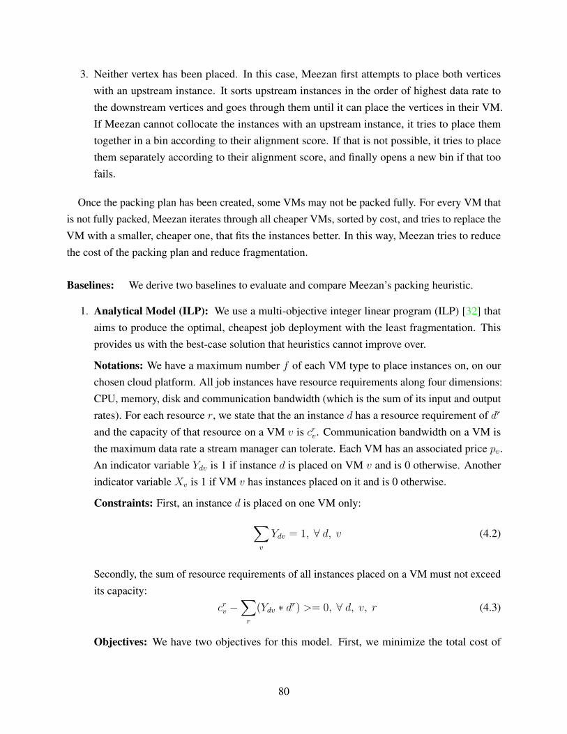
3. Neither vertex has been placed. In this case, Meezan first attempts to place both verticeswith an upstream instance. It sorts upstream instances in the order of highest data rate tothe downstream vertices and goes through them until it can place the vertices in their VM.If Meezan cannot collocate the instances with an upstream instance, it tries to place themtogether in a bin according to their alignment score. If that is not possible, it tries to placethem separately according to their alignment score, and finally opens a new bin if that toofails.

Once the packing plan has been created, some VMs may not be packed fully. For every VM thatis not fully packed, Meezan iterates through all cheaper VMs, sorted by cost, and tries to replace theVM with a smaller, cheaper one, that fits the instances better. In this way, Meezan tries to reducethe cost of the packing plan and reduce fragmentation.

Baselines: We derive two baselines to evaluate and compare Meezan’s packing heuristic.

1. Analytical Model (ILP): We use a multi-objective integer linear program (ILP) [32] thataims to produce the optimal, cheapest job deployment with the least fragmentation. Thisprovides us with the best-case solution that heuristics cannot improve over.

Notations: We have a maximum number f of each VM type to place instances on, on ourchosen cloud platform. All job instances have resource requirements along four dimensions:CPU, memory, disk and communication bandwidth (which is the sum of its input and outputrates). For each resource r, we state that the an instance d has a resource requirement of dr

and the capacity of that resource on a VM v is crv. Communication bandwidth on a VM isthe maximum data rate a stream manager can tolerate. Each VM has an associated price pv.An indicator variable Ydv is 1 if instance d is placed on VM v and is 0 otherwise. Anotherindicator variable Xv is 1 if VM v has instances placed on it and is 0 otherwise.

Constraints: First, an instance d is placed on one VM only:∑v

Ydv = 1, ∀ d, v (4.2)

Secondly, the sum of resource requirements of all instances placed on a VM must not exceedits capacity:

crv −∑r

(Ydv ∗ dr) >= 0, ∀ d, v, r (4.3)

Objectives: We have two objectives for this model. First, we minimize the total cost of

80

deployment.Cost =

∑v

(Xv ∗ pv) (4.4)

Second, we minimize the total number of VMs used, to reduce fragmentation:

Total V Ms Used =∑v

Xv (4.5)

This is essentially a problem of packing multi-dimensional balls into a minimal set of binswhich is known to be NP-Hard [162]. In order to solve this problem in a reasonable amountof time, we fix the f i.e., the number of each VM type that is supplied as input to the problem.However, we note that by doing so, we limit the optimization problem’s input, thereby gettingsolutions that may not be optimal globally.

2. Resource Compliant Round Robin (RCRR): The best packing policy Heron comes withby default is RCRR. This policy essentially places all instances of a job in a round robinmanner, across all given bins, while making sure that the capacity of any of the bins is notviolated. However, by default, the user has to specify the resource requirements of eachinstance, and the number of VMs.

Confusion has been observed anecdotally amongst engineers as the API for the policy alsoallows users to set both the maximum number of instances per VM as well as the size ofthe VM. This is odd, as if the number of VMs and instance size is specified, the sizes of theVMs required can be derived from the instances placed on them. Additionally, the API limitsusers to specify one VM size only that is meant to be used as the default size of all VMs.Furthermore, the policy has no conception of modelling data rates as one of the resources.

We modify this policy to accept the resource requirements of each instance, as derived byMeezan’s profiler, and the maximum number of bins given by the ILP. However, as a roundrobin policy does not pack instances efficiently, it is possible that the exact VMs derivedfrom the ILP may not be sufficient for all the instances to be placed in a round robin manner.Therefore, we specify the number of VMs for RCRR as the number derived by the ILP,however we provide RCRR with VMs of the largest available size on the chosen cloudplatform so that none of the instances are left unplaced.

4.4 EVALUATION

In evaluating Meezan, we are interested in answering the following questions:

81

• To what extent does Meezan minimize the cost of resources (or VMs) used on cloud platforms?

• What extent are resources fragmented to with Meezan as compared to other packing algo-rithms?

• Does Meezan successfully ensure that the stream manager per VM does not become athroughput bottleneck?

4.4.1 Evaluation Setup

In order to answer these questions, we select several real world workloads to evaluate Meezan.Our first workload is the linear road benchmark [54] which consists of three jobs and is also

employed by several previous works to evaluate improvements in stream processing systems [93,169]. It models a road toll network, in which tolls depend on the time of day and level of congestion.It specifies the following queries: (i) detect accidents on the highways (LRB Accident Detection),(ii) notify other drivers of accidents (LRB Accident Notification), and (iii) notify drivers of tollsthey have to pay (LRB Toll Calculation). Each of these benchmarks is run as a single topology,where a single spout is responsible for generating the stream of traffic per highway. As we increasethe number of spouts, we are able to process information for proportionally more highways. Thefirst two topologies are linear, with depths of 3 and 4, whereas the LRB Toll Calculation job hasjoins and a depth of 5.

We use the Yahoo! Streaming Benchmark [151] as our second workload, which models asimple advertisement application. This a linear topology with a depth of 6. There are a numberof advertising campaigns, and a number of advertisements for each campaign. The job of thebenchmark is to read JSON events, identify them, and store a windowed count of relevant eventsper campaign into Redis. These steps attempt to probe some common operations performed on datastreams. As we scale up the number of spouts, we are able to process proportionally more events.

As our final two workloads, we use 1) a 2-stage Word Count topology that has been used byseveral previous works [75,103] and produces words whose frequency is subsequently counted, and2) a similar Exclamation Topology that appends punctuation to sentences (also used in Figure 4.4a),to evaluate the systems under consideration.

We run our evaluation on a 30-node cluster on Emulab, where we provide each job the samechoices of VMs that are available to users on AWS [3].

4.4.2 Implementation

Meezan is integrated into Apache Heron [112], as a scheduler. It is an implementation of thepredefined IScheduler. It starts up as a service that profiles major VM types on given cloud platforms

82

to understand the maximum throughput rates stream managers can tolerate on them (Section 4.3.3).This is performed only once during startup, and can be repeated if new VM types are added.

When users submit jobs for deployment, they can specify Meezan as their scheduler of choice inconfiguration. During job deployment, Meezan expects that users will provide jobs that implementa predefined interface, that essentially allows Meezan to modify the amount of resources andparallelism allocated to each job operator. Once jobs are submitted to Meezan, it utilizes this flexibleconfigurability to profile the job to find it’s optimal resource allocation (Section 4.3.2.) Given theresults of profiling, Meezan produces its cost-performance spectrum for the job (Section 4.3). Theuser can then choose a job deployment that satisfies their throughput goals and falls within theirbudget, and Meezan submits their job for deployment on the relevant infrastructure of the user’scloud platform. Currently, we allow deployment on Emulab, however, hooks can be added fordeployment on AWS, Azure and Google Cloud.

4.4.3 Cost Benefits

One of the main goals of Meezan was to provide users with an array of deployment choices ofvarious costs and performance guarantees to choose from. We evaluate how the cost of a job’sdeployment increases as we scale it out with Meezan, and compare it to the optimal deploymentcost. Results for each of our benchmark jobs are shown in Figure 4.8. The y-axis shows the job’sscale (or the number of spouts it is consuming data from) and the x-axis represents the total dollarcost of deployment for an hour. We note that in most cases, the cost of deployment provided byMeezan is comparable to that of the cost provided by the ILP, when the largest (=25) frequencyof each VM type is provided to it. This essentially means that the ILP is able to optimize cost themost when it has more VMs to choose for placement. Concretely, when number of VMs providedto the ILP is 25 and the number of spouts for each job are 10, Meezan and the ILP’s deploymentcost for the Accident Detection Topology are the same = $36.29. In the same circumstances, thecost for the Accident Notification topology given by the ILP is $79.16, and Meezan’s cost is $80.21.We observe the largest difference with the Yahoo! Advertising Topology, where Meezan’s cost is$34.37 and the cost provided by the ILP is $28.44, which is a 20.85% degradation.

Readers will notice that we do not provide a cost comparison as jobs scale beyond 40 spouts atmost. This is because beyond 60 spouts, we found that solving the ILP took an exorbitant amountof time, as shown in Figure 4.9. Generally, we note that as the job size increases and the numbereach VM type provided to the ILP increases, computation time increases. In reasonable cases, suchas the the WordCount Topology scenario described above, Gurobi took 2.8 minutes to solve theproblem. In extreme cases such as for the advertising topology, given 25 of each VM types and ajob scale of 10 spouts, Gurobi took approximately 75 minutes to solve the problem.

83

(a) Advertising Topology (b) Exclamation Topology (c) Word Count Topology

(d) LRB AccidentDetection

(e) LRB AccidentNotification

(f) LRB TollCalculation

Figure 4.8: Meezan vs ILP in terms of dollar cost of job deployment. Y-axis indicates increasing number ofjob spouts. The legend indicates (Scheduler type, Number of each VM Type provided to the ILP). AsMeezan is not constrained in terms of the number of VMs it can use, we use 0 for VM frequency.

84

(a) Advertising Topology (b) Exclamation Topology(c) Word Count

Topology

(d) LRB AccidentDetection

(e) LRB AccidentNotification

(f) LRB TollCalculation

Figure 4.9: Time required by Gurobi to solve the ILP for different workloads, with each varying frequenciesof available VMs (from 3 to 25 of each type).

85

Readers will also notice that some costs of deployments are not provided (e.g., for the LRBAccident Detection Topology, where spouts = 30, and frequency of VMs = 3). In such cases, findinga solution was infeasible as even if all the given VMs were used, resources were insufficient fordeployment of the entire job.

4.4.4 Fragmentation

Figure 4.10: Fragmentation of resources in deployments of Meezan vs ILP in the Yahoo! AdvertisingTopology

We show figures 4.12-4.11 that depict the degree of fragmentation or wasted resources perdeployment in the cases of the LRB Toll Calculation, the Advertising Topology and the Word CountTopology, which are representative of the remaining cases. The y-axis represents the ratio of each ofthe unused resources per VM to the amount available in the VM. In figures 4.10 and 4.12, we notethat that the data rate of the stream manager is almost fully consumed, leading to fragmentation ofCPU and memory resources. This essentially confirms that the instances placed in each of the VMsare communication-intensive. Figure 4.12 is a particularly pathological case where one instance isplaced per VM, as that instance consumes more than half of the VM’s data rate. Therefore, CPU,memory and some of the stream manager’s resources are fragmented.

Next, we note that Meezan’s fragmentation is close to or better than that of the optimal config-urations. We compare the product of the ratios of each of the fragmented resources per policy toevaluate this. In the best case, we note in the best case of the Toll Calculation Topology where thenumber of spouts = 10 and the frequency of VMs is 10 for the ILP, the fragmentation in Meezan’s

86

Figure 4.11: Fragmentation of resources in deployments of Meezan vs ILP in the Word Count Topology.The legend indicates (Scheduler type, Number of each VM Type provided to the ILP).

Figure 4.12: Fragmentation of resources in deployments of Meezan vs ILP in the LRB Toll CalculationTopology. The legend indicates (Scheduler type, Number of each VM Type provided to the ILP).

deployment is 0.76 vs the 0.97 fragmentation given by the ILP, which is a 27% improvement. In theworst case of the Advertising Topology, with 3 spouts, and frequency of 10 VM types, Meezan does15% worse than the ILP. (Meezan’s fragmentation is 0.9 and the ILP’s fragmentation is 0.78).

87

4.4.5 Throughput

(a) Yahoo! Advertising Benchmark (b) Exclamation Topology (c) WordCount Topology

(d) LRB Accident Detection (e) LRB Accident Notification (f) LRB Toll Calculation

Figure 4.13: Meezan vs ILP in terms of average throughput per-spout for varying workloads as they arescaled out.

Meezan aims to pack instances onto VMs while ensuring that the stream manager in each VM isnot bottlenecked by extremely high throughput. Therefore, as we scale jobs out from having 1 to 10spouts, and pack them onto VMs, we evaluate the average throughput of each spout in each job andpresent them in Figure 4.13. If Meezan does its job correctly, the average throughput per spoutsshould remain in the same range. We notice that the average throughput across all spouts in theLRB topologies are similar to each other, irrespective of scheduler choice. This is because eachof the spouts performs some computation to generate the LRB workload, which means that theirthroughput is not high enough to bottleneck the stream manager. This means that regardless of thepacking policy, the average throughput per spout remains high.

The Advertising Topology, Exclamation Topology and Word Count Topology all have highthroughput rates. In the case of the advertising topology and the exclamation topology, we note thatMeezan and the ILP are able to maintain the throughput of each spout to the average produced by asingle spout. However, we notice that as RCRR places instances in bins in a round robin fashion,

88

it instances together, causing the stream manager to become a bottleneck. We notice thus that theaverage throughput per spout with RCRR falls up to 43% in the case of the Advertising Topologyand the Exclamation topology.

In the Word Count Topology, we note that RCRR does as well as Meezan. This is because theRCRR is given a very high number of VMs to use (from the ILP, which essentially packs oneoperator per VM). Because of the large number of VMs available that RCRR must use, it packsone operator per VM. As a result, the stream manager is not bottlenecked and its throughput levelsremain high on average.

4.5 RELATED WORK

4.5.1 Stream Processing as a Service

Amazon Kinesis [2] offers itself as a Streaming as a Service Platform. It enables easy collection,processing and analysis of real-time streaming data. However, the system leaves performance tuningof the job up to the user. In Amazon Kinesis, each data stream is a function of the number of shardsthat the user specifies for the stream. The total capacity of the stream is the sum of the capacitiesof its shards. As the input data rate changes, the user needs to increase or decrease the number ofshards to maintain throughput. Our goal is to remove this burden from the user’s shoulders.

4.5.2 Optimal Resource Allocation in Distributed Systems

Perforator [140] is one of the first systems that tackles the resource allocation problem for DAGsof batch-compute jobs. It models, first, the estimated size of input data that the job must process andsecond, the job’s performance, by analyzing results of hardware calibration queries, and using themto ascertain the parallelism of tasks in the execution frameworks. Ernest [158] is a performanceprediction framework for batch jobs, that uses optimal experiment design. This is a statisticaltechnique that allows its users to collect as few training points as possible, that indicate how shortruns of each incoming jobs perform on specific hardware. These training points can be used tomodel the performance of these jobs on specific hardware, with larger input sizes, that can be usedto predict near-optimal resource allocations for them. Cherrypick [49] is a system that leveragesBaysian Optimization, a method for optimizing blackbox functions, to find near-optimal cloudconfigurations that minimize cloud usage cost and guarantee application performance for generalbatch-compute applications. The main idea of Cherrypick works as follows: start with a few initialcloud configurations, run them, and input the configuration details and job completion time into theperformance model. The system then dynamically pick the next cloud configuration to run based on

89

the performance model and feed the result back to the performance model. The system stops whenit has enough confidence a good configuration has been found.

The problem of finding optimal resource allocation for jobs has also been explored in otherdistributed systems such as systems for deep learning. FlexFlow [98] is a deep learning engine thatemploys a guided randomized search to quickly find a parallelization strategy of a deep learningtraining job for a specific parallel machine. In order to do so, FlexFlow first borrows the idea ofmeasuring the performance of an operator once for each configuration from OptCNN [97], which isa similar approach to Meezan, and feeds these measurements into a task graph that models both thearchitecture of a DNN model and the network topology of a cluster.

Fine-grained resource allocation is also studied for micro-service architectures. MONAD [132]is a self-adaptive infrastructure for micro-services that are meant to run heterogeneous scientificworkflows. Using fine-grained scheduling at the task-level, MONAD improves the flexibility ofworkflow composition and execution, It also shares tasks between multiple workflows. Furthermore,it uses feedback control with neural network-based system identification to provide resourceadaptation without in-depth knowledge of workflow structures.

The problem of minimizing deployment cost exists in many domains, including serverlesscomputing, that is used to process data across the edge and in data centers. Costless [73] presentsan algorithm that optimizes the price of serverless applications on Amazon AWS Lambda. Thepaper describes factors that affect the price of a deployment: (1) fusing a sequence of functions, (2)splitting functions across edge and cloud resources, and (3) allocating the memory for each function.Costless runs an efficient algorithm to explore different function fusion-placement solutions andchoose one that optimizes the application’s price while keeping the latency under a certain threshold.

4.5.3 Video Stream Processing

Video stream processing jobs require additional effort to minimize the massive computationalcost of performing computer vision tasks that Meezan does not take into account so far. For example,one work [94] asks whether video analytics can be scaled in a way that cost grows sublinearly,as more video cameras are deployed and inference accuracy of processing remains stable. Toachieve their goal, the authors observe that video feeds from wide-area camera deploymentsdemonstrate significant content correlations to other geographically proximate feeds, both spatiallyand temporally. These correlations can be harnessed to dramatically reduce the size of the inferencesearch space, decreasing both workload and false positive rates in multi-camera video analytics.

This problem is also explored for environments where video stream processing jobs are deployedon a hierarchy of clusters. VideoEdge [91] is a system that uses the concept of “dominant” demandto identify the best tradeoff between multiple resources and accuracy, and narrows the search

90

space for placement on a hierarchical set of clusters, by identifying a “Pareto band” of promisingconfigurations. The system also balances the resource benefits and accuracy penalty of mergingqueries.

4.5.4 Performance Modelling of Message Brokers

Balasubramanian [56] model a scenario in publish-subscribe systems where the publishers, thebroker, and the subscribers are in different administrative domains and have no guarantees withrespect to the resources available to each service. Within this context, they focus on dynamicallyadapting the amount of data that the publishers send to the brokers to prevent backpressure at thebrokers. Nguyen [131] model publish-subscribe systems as multiple-class open queueing networksto derive measures of system performance. Using these measures, they solve objective functionsthat have the goal of either minimizing the latency for processing an input which translates tofinding the optimal number of consumers in the system or finding the least end-to-end latency thatcan be provided while minimizing the total resource cost of consumers in the system. The formerproblem is the same as calculating the parallelism of downstream bolts in a continuous-operatorstream processing topology.

To the best of our knowledge, these are the only work that experimentally evaluates the perfor-mance of recent message brokers such as Apache Kafka [111].

4.5.5 Backpressure in networks

The slowdown of upstream operators in Heron jobs because of a bottlenecked stream managercan be likened to the backpressure exerted in networks due to congestion control [50]. However,the two scenarios have different solutions because the causes of their bottlenecks are different:congestion in networks is caused by limited bandwidth [134] (if the network configuration is correctand well-designed), while stream manager slowdown is caused by a lack of computational resources.Therefore, Meezan removes the stream manager bottleneck by ensuring that each stream manager isnot oversubscribed, and only receives as much data as it is able to transfer per unit time. Meezan’sscope does not include handling network-related backpressure.

4.5.6 Scaling in Stream Processing Systems

A great deal of research considers the problem of scaling resources in and out to meet performancegoals in stream processing systems. Drizzle [157] adapts the size of the batch in micro-batch streamprocessing systems such as Spark Streaming [168] to provide low latency and high throughput. DRS

91

[76] has applied queueing theory to create performance models for continuous-operator streamprocessing systems that do not have intermediate message brokers such as Apache Storm [154]. TriMinh et al. [155] consider the performance of stream processing systems in terms of back-pressureand expected utilization. They focus on a queueing theory-based approach that is used to predictthe throughput and latency of stream processing while supporting system stability in the face ofbursty input.

Dhalion [75] proposes the use of self-regulating stream processing systems and provides aprototype with some capabilities that can diagnose problems e.g., backpressure in Heron topologiesand can take actions to mitigate the problem. It’s corrective actions are heuristics, however,DS2 [102] provides scaling methods that are based on precise processing and output rates ofindividual dataflow operators. Henge [104] supports SLO-driven multi-tenancy in clusters of limitedresources.

Authors of [59] use a hill-climbing algorithm that uses a new heuristic sampling approach basedon Latin Hypercube to automate the process of tuning some of the configuration parameters ofcontinuous-operator systems like Apache Storm [154]. However, the work is not able to cover amajority of the parameters that need to be tuned for optimal performance.

Trevor [58] is parallel work that focuses on auto-configuring stream processing jobs especiallythose run on Apache Heron. Like [103], it builds a simple model that compares an instance’s inputrate with its output rate to model the instance’s behavior and uses heuristics to ensure that eachstream manager per container is not bottle-necked. However, it does not aim to minimize the amountof resources used by job or lower the cost of running the job for the user.

4.6 CONCLUSION

Meezan is a scheduler for stream processing systems that provides users with a range of possibledeployments for their jobs. Each deployment has a different price and a different performanceguarantee. The most performant choice is associated with the highest cost and vice versa. Wecompare Meezan with a multi-objective optimization framework that given a job DAG and a fixedset of VMs, optimizes the total cost of deployment and minimizes the number of containers usedfor a job. Meezan is able to ensure that the choice of deployment it provides users with is within20.85% of cost found by the optimization problem. Additionally, as it is able to open up bins of itschoice while the optimization framework is limited to a fixed set of bins, it is able to reduce resourcefragmentation by up to 27% over the framework’s solution. While packing, Meezan ensures that itdoes not allow jobs to be bottlenecked by components that are transparent to the job developer, andensures that as jobs scale up, their average throughput increases in proportion to their scale.

92

Chapter 5: Conclusion and Future Work

Even though stream processing systems have become increasingly prevalent with the increaseduse of applications that require low-latency responses, they still face several challenges in terms ofachieving performance goals in different scheduling environments. In multi-tenant environmentswith limited shared resources, jobs have to be assigned resources after carefully considering theirjob complexity, priorities and performance requirements. These resource allocations must changeover time as jobs receive input at varying rates. On the other hand, while scheduling jobs onto publiccloud services such as Amazon AWS [3] or Microsoft Azure [30] where resources are virtuallyunlimited, we must carefully determine the most optimal VM choices in terms of cost and resources,that will help us achieve our performance goals. Such problems motivate the need for both onlineand predictive mechanisms that determine optimal resource allocations for jobs before they arelaunched, and continue to adapt their allocations to dynamically changing conditions.

In this thesis, we present practical techniques for achieving performance goals or Service LevelObjectives (SLOs) [38] in stream processing systems that are used by a variety of users in differentdata center environments.

1. Henge [104] is an online scheduler for stream processing systems that addresses the challengeof adapting job resource allocations in a multi-tenant environment with limited resources tomaximize cluster utility. It does so by ensuring that the SLOs of higher priority jobs thatprovide higher utility to the organization are met first, and if resources are available, ensuresthat the SLOs of lower priority jobs are also met. Henge reduces intrusiveness by making theleast number of modifications it can to each job. In addition, we show that Henge convergesprovably if job input rates stabilize i.e. once input rates of all jobs stabilize, Henge is alwaysable to find a resource allocation for all jobs in the cluster that maximize cluster utility.

2. Caladrius [103] is a scheduler for stream processing jobs that is built in collaboration withTwitter that predicts changes in the input rates of a job and scales it out (or in) preemptivelyto ensure that the job’s throughput SLOs are always met, while reducing resource wastage. Inorder to make predictions of future input rates, Caladrius uses Facebook’s Prophet [34], atime-series forecasting tool that is optimized for predicting observations that depict stronghuman-scale seasonalities, which our experience at Twitter shows that stream processingjobs most often do. Given these forecasted changes, Caladrius models components in the jobgraphs and recalculates their parallelism levels to ensure that they are not bottlenecked becauseof predicted increases in input rate. Based on the job’s new parallelism level, Caladrius derivesa new resource allocation for the job to which it can be scaled out preemptively to ensure thatthe job does not miss its SLO at any point in time.

93

3. Meezan allows novice users of stream processing jobs to select a resource allocation of theirstream processing job on public cloud services that will meet their throughput-based perfor-mance goals while reducing cost of deployment. In Meezan, we present two contributions: 1)we present a case study that models how dedicated VMs are priced on Amazon and Azure,and using insights from our study, 2) we propose a novel packing algorithm that minimizesthe cost of job deployments on these platforms, while ensuring that the job’s throughput SLOis met. A fundamental contribution of our packing algorithm is that it takes components ofjob graphs into account that are transparent to the job developer but are fundamental to thejob’s function, such as message brokers that are responsible for data transmission among thejob’s components.

The steps needed to deploy jobs per environment are described in each system’s respective chapter.To production-ize these systems, some engineering work is required to hook them up with existingcompany infrastructure.

This thesis lays the ground work for several future directions:

Message Brokers as In-Network Components: In recent years, the academic communityhas proposed using in-network computation to implement a vast variety of functionality that isnormally performed by systems [138]. This includes concurrency control [96, 115], aggregationprimitives [143], consensus protocols [67, 68, 116, 137], and query processing operators [83, 113].Other work offloads entire applications to programmable devices, including key-value stores [153],network protocols like DNS [153], and even industrial feedback control [142].

We note through Meezan that Heron topologies have a stream manager that is a great candidatefor in-network processing. We observe that the stream manager is responsible for receiving datafrom local operators and passing it on to other destination operators that are either local or areremote. If the operators are placed remotely, a stream manager simply passes the data to the streammanager that is local to the destination operator, and that stream manager passes the data onto to thelocal operator. Therefore, we observe that the role of the stream manager is very much like that of anetwork switch. It is also a good candidate for in-network processing as it is not performing complexcomputation on data: it has been designed to simplify the role of operators, so that operators donot maintain connections with remote operators and simply pass the data to the stream manager.Additionally, the stream manager also must only maintain connections with local operators andremote stream managers, instead of maintaining connections with all operators. The essential workthe stream manager is doing is determining which data packet should be sent to which destination,and batching it together to be sent to the recipient. By moving this task to the network, we cansave on the cost of moving data from the transport layer to the application layer, where it has to bedeserialized to be read. This can potentially lead to significant reductions on end-to-end latency of a

94

tuple as it moves throughout the topology, especially as we note that there can be multiple streammanagers in its path.

Satisfying Global Latency SLOs: In this thesis, we have defined latency SLOs with respect tothe amount of time it takes a tuple to be processing fully in a stream processing topology running ina data center. However, most stream processing applications process data that arrives into the datacenters from across the world and require that responses that should be sent received at the senderwithin a few seconds. Such “global” latency goals can be very business-critical. For example, if aride-sharing app is not able to send a response back to a rider with a driver match in a few seconds,it risks losing the rider to a competitor [28]. However, in situations where requests and responses aresent over the WAN, network congestion can create difficulties in promising low latencies [60, 100].A possible future direction of this thesis is to derive minimum and maximum latency SLOs that canbe guaranteed to the users and can be met with a defined degree of reliability.

Stream Processing as SIMD Applications: Stream processing jobs are applications that can benaturally run on SIMD (Single Instruction, Multiple Data [37]) architectures, as their job operatorsinvolve applying the same instruction to multiple pieces of incoming data. This means that wecan easily use GPUs to speed up the performance of stream processing applications to meet SLOs,especially those running on micro-batch streaming architectures [69] such as Spark Streaming [168],which attempt to process small batches of data at a time. An interesting direction would involvediscovering the extent to which we can automatically translate a given application’s code that ismeant to run on a CPU to one that would run as a SIMD application. For instance, operations suchas joins would not be sped up by using GPUs.

Defining Fairness in Multi-Tenant Stream Processing Clusters: Defining fair-shares of tasksin a distributed systems is challenging and some works have explored fairness in batch data analyticssystems [80, 81]. This task is challenging because although fairness requires an “equal” share ofresources across jobs, one job’s share might be an excess for it, whereas another job’s share mightnot even be enough for a single operator of the job. However, fairness is important, especially instream processing as jobs are long-running and even some amount of starvation can lead to backlogsof data.

In Henge, we define fairness in accordance with a job’s priority. In batch computation, severalfairness-related measures have been developed such as dominant resource fairness [80], whichare not directly applicable as a stream processing jobs face more dynamism and their dominantresource share might change over time. Therefore, a possible future direction is to express fairnessbased on performance goals – for example, a fair allocation would be where all jobs of the same

95

priority achieve the same percentage of their performance goal – and to describe it’s fair-divisionproperties [61].

Generalizing Workloads, Job Components, and Resources:Machine Learning Inference Workloads: Stream processing jobs can mirror the behavior of

other long running jobs such as machine learning inference jobs. However, the computation inmachine learning DAGs can be quite different from the general operators used in stream processing.In addition, they can also require the usage of more heterogeneous resources such as GPUs andTPUs [14]. A possible future direction is to meet define and achieve SLOs of ML inference jobs indifference cloud environments. Although this topic has begun to gain traction very recently [82,171],an interesting direction is to adaptively move inference components from data center environmentsto edge devices [144] in order to reduce end-to-end latency.

External Bottlenecks: In the same vein, another possible future direction is to evaluate systemssuch as Apache Samza [6] and Flink [4] that utilize message brokers e.g., Apache Kafka [111], inplace of stream managers in stream processing systems. As these message brokers also write data todisk, they can be IO bound, and can form potential bottlenecks in stream processing jobs that havestrict, low latency SLOs. A possible direction of future work is to determine the optimal number ofpartitions and message brokers for a job to achieve both its latency or throughput SLO.

Dynamically Changing DAGs: Within this thesis, we focus on stream processing DAGs thatdo not change at runtime. However, in production deployments, it is possible that operators aredynamically added to jobs to deal with challenges at runtime, such as unexpectedly high input andfailures. It is also common that such dynamic additions are short-lived. An interesting direction toexplore is A) when are such dynamic changes necessitated and when should they be added, and B)how do allocate these operators to maximize resource utilization and reduce deployment cost.

Theoretical Guarantees An interesting obstacle for using Meezan in production is that usershave to be convinced of its efficacy in order to allow it to make decisions based for them, that costthem real money. For example, given that Netflix has thousands of data shards (streams) cominginto AWS Kinesis (a streaming platform on AWS) daily [33], we can estimate that they spend($0.36 (cost per day) × 1000 (streams) × 30 (days in a month)) = $10,800 per month for only athousand streams [9]. As these numbers are quite large, it is natural that user’s would like assurancethat Meezan’s packing policy minimizes cost of deployment. In order to overcome this obstacle, apossible future work is to derive theoretical bounds for the best and worst cases that Meezan canprovide.

96

References

[1] Amazon EC2 Pricing. https://aws.amazon.com/ec2/pricing/on-demand/.Last Visited: Sunday 12th July, 2020.

[2] Amazon Kinesis. https://aws.amazon.com/kinesis/data-streams/faqs/.Last Visited: Sunday 12th July, 2020.

[3] Amazon Web Services. https://aws.amazon.com/. Last Visited: Sunday 12th July,2020.

[4] Apache Flink. http://flink.apache.org/. Last Visited: Sunday 12th July, 2020.

[5] Apache Flume. https://flume.apache.org/. Last Visited: Sunday 12th July, 2020.

[6] Apache Samza. http://samza.apache.org/. Last Visited: 03/2016.

[7] Apache Storm. http://storm.apache.org/. Last Visited: Sunday 12th July, 2020.

[8] Apache Zookeeper. http://zookeeper.apache.org/. Last Visited: Sunday 12th

July, 2020.

[9] AWS Kinesis Pricing. https://aws.amazon.com/kinesis/data-streams/pricing/. Last Visited: Sunday 12th July, 2020.

[10] CPU Load. http://www.linuxjournal.com/article/9001. Last Visited: Sun-day 12th July, 2020.

[11] EC2 Instance Types. https://www.ec2instances.info/?selected=g4dn.2xlarge. Last Visited: Sunday 12th July, 2020.

[12] Elasticity in Spark Core. http://www.ibmbigdatahub.com/blog/explore-true-elasticity-spark/. Last Visited: Sunday 12th July, 2020.

[13] EPA-HTTP Trace. http://ita.ee.lbl.gov/html/contrib/EPA-HTTP.html.Last Visited: Sunday 12th July, 2020.

[14] Google Cloud TPU. https://cloud.google.com/tpu. Last Visited: Sunday 12th

July, 2020.

[15] Heron Github Issue 1125. https://github.com/apache/incubator-heron/issues/1125. Last Visited: Sunday 12th July, 2020.

[16] Heron Github Issue 119. https://github.com/apache/incubator-heron/issues/119. Last Visited: Sunday 12th July, 2020.

[17] Heron Github Issue 1389. https://github.com/apache/incubator-heron/issues/1389. Last Visited: Sunday 12th July, 2020.

97

[18] Heron Github Issue 1577. https://github.com/apache/incubator-heron/issues/1577. Last Visited: Sunday 12th July, 2020.

[19] Heron Github Issue 1888. https://github.com/apache/incubator-heron/issues/1888. Last Visited: Sunday 12th July, 2020.

[20] Heron Github Issue 1947. https://github.com/apache/incubator-heron/issues/1947. Last Visited: Sunday 12th July, 2020.

[21] Heron Github Issue 2454. https://github.com/apache/incubator-heron/issues/2454. Last Visited: Sunday 12th July, 2020.

[22] Heron Github Issue 266. https://github.com/apache/incubator-heron/issues/266. Last Visited: Sunday 12th July, 2020.

[23] Heron Github Issue 2803. https://github.com/apache/incubator-heron/issues/2803. Last Visited: Sunday 12th July, 2020.

[24] Heron Github Issue 3396. https://github.com/apache/incubator-heron/issues/3396. Last Visited: Sunday 12th July, 2020.

[25] Heron Github Issue 3494. https://github.com/apache/incubator-heron/issues/3494. Last Visited: Sunday 12th July, 2020.

[26] Heron Github Issue 3504. https://github.com/apache/incubator-heron/issues/3504. Last Visited: Sunday 12th July, 2020.

[27] Heron Trouble Shooting. https://apache.github.io/incubator-heron/docs/developers/troubleshooting/. Last Visited: Sunday 12th July, 2020.

[28] Introducing AthenaX, Uber Engineering’s Open Source Streaming Analytics Platform.https://eng.uber.com/athenax/. Last Visited: Sunday 12th July, 2020.

[29] Kafka Streams. https://kafka.apache.org/documentation/streams/.Last Visited: Sunday 12th July, 2020.

[30] Microsoft Azure. https://azure.microsoft.com/en-us/. Last Visited: Sunday12th July, 2020.

[31] Microsoft Azure: Linux Virtual Machines Pricing. https://azure.microsoft.com/en-us/pricing/details/virtual-machines/linux/. Last Visited: Sunday12th July, 2020.

[32] Multi-Objective Optimization. https://en.wikipedia.org/wiki/Multi-objective_optimization. Last Visited: Sunday 12th July, 2020.

[33] Netflix Streaming Use Cases. https://aws.amazon.com/solutions/case-studies/netflix-kinesis-streams/. Last Visited: Sunday 12th

July, 2020.

98

[34] Prophet: Forecasting at Scale. https://research.fb.com/blog/2017/02/prophet-forecasting-at-scale/. Last Visited: Sunday 12th July, 2020.

[35] S4. http://incubator.apache.org/s4/. Last Visited: 03/2016.

[36] SDSC-HTTP Trace. http://ita.ee.lbl.gov/html/contrib/SDSC-HTTP.html. Last Visited: Sunday 12th July, 2020.

[37] SIMD. https://en.wikipedia.org/wiki/SIMD. Last Visited: Sunday 12th July,2020.

[38] SLOs. https://en.wikipedia.org/wiki/Service_level_objective.Last Visited: Sunday 12th July, 2020.

[39] Storm 0.8.2 Release Notes. http://storm.apache.org/2013/01/11/storm082-released.html/. Last Visited: Sunday 12th July, 2020.

[40] Storm Applications. http://storm.apache.org/Powered-By.html. Last Vis-ited: Sunday 12th July, 2020.

[41] Storm MultiTenant Scheduler. http://storm.apache.org/releases/2.0.0-SNAPSHOT/SECURITY.html. Last Visited: Sunday 12th July, 2020.

[42] Uber Streaming Use Cases. https://www.youtube.com/watch?v=YUBPimFvcN4. Last Visited: Sunday 12th July, 2020.

[43] Why Multitenancy Matters In The Cloud. https://en.wikipedia.org/wiki/Multitenancy#Cost_savings. Last Visited: Sunday 12th July, 2020.

[44] Zillow Streaming Use Cases. https://aws.amazon.com/solutions/case-studies/zillow-zestimate/. Last Visited: Sunday 12th July, 2020.

[45] Daniel Abadi, Donald Carney, Ugur Cetintemel, Mitch Cherniack, Christian Convey, C Erwin,Eduardo Galvez, M Hatoun, Anurag Maskey, Alex Rasin, et al. Aurora: A Data StreamManagement System. In Proceedings of the International Conference on Management ofData (SIGMOD), pages 666–666. ACM, 2003.

[46] Daniel J Abadi, Yanif Ahmad, Magdalena Balazinska, Ugur Cetintemel, Mitch Cherniack,Jeong-Hyon Hwang, Wolfgang Lindner, Anurag Maskey, Alex Rasin, Esther Ryvkina, et al.The Design of the Borealis Stream Processing Engine. In Proceedings of the Conference onInnovative Data Systems Research, volume 5, pages 277–289, 2005.

[47] Tyler Akidau, Alex Balikov, Kaya Bekiroglu, Slava Chernyak, Josh Haberman, Reuven Lax,Sam McVeety, Daniel Mills, Paul Nordstrom, and Sam Whittle. Millwheel: Fault-TolerantStream Processing at Internet Scale. In Proceedings of the VLDB Endowment, volume 6,pages 1033–1044. VLDB Endowment, 2013.

99

[48] Tyler Akidau, Robert Bradshaw, Craig Chambers, Slava Chernyak, Rafael J Fernández-Moctezuma, Reuven Lax, Sam McVeety, Daniel Mills, Frances Perry, Eric Schmidt, et al. Thedataflow model: a practical approach to balancing correctness, latency, and cost in massive-scale, unbounded, out-of-order data processing. Proceedings of the VLDB Endowment,8(12):1792–1803, 2015.

[49] Omid Alipourfard, Hongqiang Harry Liu, Jianshu Chen, Shivaram Venkataraman, MinlanYu, and Ming Zhang. Cherrypick: Adaptively Unearthing the Best Cloud Configurationsfor Big Data Analytics. In 14th {USENIX} Symposium on Networked Systems Design andImplementation ({NSDI} 17), pages 469–482, 2017.

[50] Mark Allman, Vern Paxson, Wright Stevens, et al. Tcp congestion control. 1999.

[51] Tanvir Amin. Apollo Social Sensing Toolkit. http://apollo3.cs.illinois.edu/datasets.html, 2014. Last Visited: Sunday 12th July, 2020.

[52] Leonardo Aniello, Roberto Baldoni, and Leonardo Querzoni. Adaptive Online Scheduling inStorm. In Proceedings of the 7th ACM International Conference on Distributed Event-BasedSystems, pages 207–218. ACM, 2013.

[53] Apache Software Foundation . Apache Kafka Supports 200K Parti-tions Per Cluster. https://blogs.apache.org/kafka/entry/apache-kafka-supports-more-partitions. Last Visited: Sunday 12th

July, 2020.

[54] Arvind Arasu, Mitch Cherniack, Eduardo Galvez, David Maier, Anurag S Maskey, EstherRyvkina, Michael Stonebraker, and Richard Tibbetts. Linear road: a stream data managementbenchmark. In Proceedings of the Thirtieth international conference on Very large databases-Volume 30, pages 480–491, 2004.

[55] Masoud Saeida Ardekani and Douglas B Terry. A Self-Configurable Geo-Replicated CloudStorage System. In Proceedings of the 11th USENIX Symposium on Operating SystemsDesign and Implementation (OSDI), pages 367–381, 2014.

[56] Sowmya Balasubramanian, Dipak Ghosal, Kamala Narayanan Balasubramanian Sharath,Eric Pouyoul, Alex Sim, Kesheng Wu, and Brian Tierney. Auto-tuned publisher in a pub/subsystem: Design and performance evaluation. In 2018 IEEE International Conference onAutonomic Computing (ICAC), pages 21–30. IEEE, 2018.

[57] Cagri Balkesen, Nesime Tatbul, and M Tamer Özsu. Adaptive Input Admission and Manage-ment for Parallel Stream Processing. In Proceedings of the 7th ACM International Conferenceon Distributed Event-Based Systems, pages 15–26. ACM, 2013.

[58] Manu Bansal, Eyal Cidon, Arjun Balasingam, Aditya Gudipati, Christos Kozyrakis, andSachin Katti. Trevor: Automatic configuration and scaling of stream processing pipelines.arXiv preprint arXiv:1812.09442, 2018.

100

[59] Muhammad Bilal and Marco Canini. Towards automatic parameter tuning of stream process-ing systems. In Proceedings of the 2017 Symposium on Cloud Computing, pages 189–200.ACM, 2017.

[60] Lawrence S. Brakmo and Larry L. Peterson. Tcp vegas: End to end congestion avoidanceon a global internet. IEEE Journal on selected Areas in communications, 13(8):1465–1480,1995.

[61] Steven J Brams and Alan D Taylor. Fair Division: From cake-cutting to dispute resolution.Cambridge University Press, 1996.

[62] Paris Carbone, Asterios Katsifodimos, Stephan Ewen, Volker Markl, Seif Haridi, and KostasTzoumas. Apache flink: Stream and batch processing in a single engine. Bulletin of the IEEEComputer Society Technical Committee on Data Engineering, 36(4), 2015.

[63] Raul Castro Fernandez, Matteo Migliavacca, Evangelia Kalyvianaki, and Peter Pietzuch.Integrating Scale-Out and Fault Tolerance in Stream Processing using Operator State Manage-ment. In Proceedings of the International Conference on Management of Data (SIGMOD),pages 725–736. ACM, 2013.

[64] Javier Cervino, Evangelia Kalyvianaki, Joaquin Salvachua, and Peter Pietzuch. AdaptiveProvisioning of Stream Processing Systems in the Cloud. In Proceedings of the 28thInternational Conference on Data Engineering Workshops, pages 295–301. IEEE, 2012.

[65] Cloudera. Tuning YARN — Cloudera. http://www.cloudera.com/documentation/enterprise/5-2-x/topics/cdh_ig_yarn_tuning.html, 2016. Last Visited Sunday 12th July, 2020.

[66] Carlo Curino, Djellel E Difallah, Chris Douglas, Subru Krishnan, Raghu Ramakrishnan, andSriram Rao. Reservation-Based Scheduling: If You’re Late Don’t Blame Us! In Proceedingsof the ACM Symposium on Cloud Computing, pages 1–14. ACM, 2014.

[67] Huynh Tu Dang, Pietro Bressana, Han Wang, Ki Suh Lee, Hakim Weatherspoon, MarcoCanini, Fernando Pedone, and Robert Soulé. Network hardware-accelerated consensus.arXiv preprint arXiv:1605.05619, 2016.

[68] Huynh Tu Dang, Pietro Bressana, Han Wang, Ki Suh Lee, Hakim Weatherspoon, MarcoCanini, Noa Zilberman, Fernando Pedone, and Robert Soulé. P4xos: Consensus as anetwork service. Technical report, Research Report 2018-01. USI. http://www. inf. usi.ch/research_publication. htm, 2018.

[69] Tathagata Das, Matei Zaharia, and Patrick Wendell. Diving into Apache SparkStreaming’s Execution Model. https://databricks.com/blog/2015/07/30/diving-into-apache-spark-streamings-execution-model.html. LastVisited: Sunday 12th July, 2020.

[70] Giuseppe DeCandia, Deniz Hastorun, Madan Jampani, Gunavardhan Kakulapati, AvinashLakshman, Alex Pilchin, Swaminathan Sivasubramanian, Peter Vosshall, and Werner Vogels.

101

Dynamo: Amazon’s Highly Available Key-Value Store. ACM SIGOPS Operating SystemsReview, 41(6):205–220, 2007.

[71] Christina Delimitrou and Christos Kozyrakis. Paragon: QoS-Aware Scheduling for Hetero-geneous Datacenters. In Proceedings of the 18th International Conference on ArchitecturalSupport for Programming Languages and Operating Systems, ASPLOS ’13, pages 77–88,New York, NY, USA, 2013. ACM.

[72] Christina Delimitrou and Christos Kozyrakis. Quasar: Resource-efficient and QoS-awareCluster Management. In Proceedings of the 19th International Conference on ArchitecturalSupport for Programming Languages and Operating Systems, ASPLOS ’14, pages 127–144,New York, NY, USA, 2014. ACM.

[73] Tarek Elgamal. Costless: Optimizing cost of serverless computing through function fusionand placement. In 2018 IEEE/ACM Symposium on Edge Computing (SEC), pages 300–312.IEEE, 2018.

[74] Huifang Feng and Yantai Shu. Study on network traffic prediction techniques. In WirelessCommunications, Networking and Mobile Computing, 2005. Proceedings. 2005 InternationalConference on, volume 2, pages 1041–1044. IEEE, 2005.

[75] Avrilia Floratou, Ashvin Agrawal, Bill Graham, Sriram Rao, and Karthik Ramasamy.Dhalion: self-regulating stream processing in heron. Proceedings of the VLDB Endow-ment, 10(12):1825–1836, 2017.

[76] Tom ZJ Fu, Jianbing Ding, Richard TB Ma, Marianne Winslett, Yin Yang, and ZhenjieZhang. DRS: Dynamic Resource Scheduling for Real-Time Analytics over Fast Streams. InProceedings of the 35th International Conference on Distributed Computing Systems, pages411–420. IEEE, 2015.

[77] Bugra Gedik, Henrique Andrade, Kun-Lung Wu, Philip S Yu, and Myungcheol Doo. SPADE:The System S Declarative Stream Processing Engine. In Proceedings of the InternationalConference on Management of Data (SIGMOD), pages 1123–1134. ACM, 2008.

[78] Bugra Gedik, Scott Schneider, Martin Hirzel, and Kun-Lung Wu. Elastic Scaling for DataStream Processing. IEEE Transactions on Parallel and Distributed Systems, 25(6):1447–1463, 2014.

[79] Javad Ghaderi, Sanjay Shakkottai, and Rayadurgam Srikant. Scheduling storms and streamsin the cloud. In ACM SIGMETRICS Performance Evaluation Review, volume 43, pages439–440. ACM, 2015.

[80] Ali Ghodsi, Matei Zaharia, Benjamin Hindman, Andy Konwinski, Scott Shenker, and IonStoica. Dominant Resource Fairness: Fair Allocation of Multiple Resource Types. In Pro-ceedings of the 8th USENIX Symposium on Networked Systems Design and Implementation(NSDI), volume 11, pages 24–24, 2011.

102

[81] Robert Grandl, Ganesh Ananthanarayanan, Srikanth Kandula, Sriram Rao, and Aditya Akella.Multi-Resource Packing for Cluster Schedulers. ACM SIGCOMM Computer CommunicationReview, 44(4):455–466, 2015.

[82] Arpan Gujarati, Sameh Elnikety, Yuxiong He, Kathryn S McKinley, and Björn B Brandenburg.Swayam: distributed autoscaling to meet slas of machine learning inference services withresource efficiency. In Proceedings of the 18th ACM/IFIP/USENIX Middleware Conference,pages 109–120, 2017.

[83] Arpit Gupta, Rob Harrison, Marco Canini, Nick Feamster, Jennifer Rexford, and WalterWillinger. Sonata: Query-driven streaming network telemetry. In Proceedings of the 2018Conference of the ACM Special Interest Group on Data Communication, pages 357–371,2018.

[84] Thomas Heinze, Zbigniew Jerzak, Gregor Hackenbroich, and Christof Fetzer. Latency-AwareElastic Scaling for Distributed Data Stream Processing Systems. In Proceedings of the 8thACM International Conference on Distributed Event-Based Systems, pages 13–22. ACM,2014.

[85] Thomas Heinze, Valerio Pappalardo, Zbigniew Jerzak, and Christof Fetzer. Auto-ScalingTechniques for Elastic Data Stream Processing. In Proceedings of the 30th InternationalConference on Data Engineering Workshops, pages 296–302. IEEE, 2014.

[86] Thomas Heinze, Lars Roediger, Andreas Meister, Yuanzhen Ji, Zbigniew Jerzak, and ChristofFetzer. Online Parameter Optimization for Elastic Data Stream Processing. In Proceedingsof the 6th ACM Symposium on Cloud Computing, pages 276–287. ACM, 2015.

[87] Herodotos Herodotou and Shivnath Babu. Profiling, what-if analysis, and cost-based opti-mization of mapreduce programs. Proceedings of the VLDB Endowment, 4(11):1111–1122,2011.

[88] Herodotos Herodotou, Fei Dong, and Shivnath Babu. No one (cluster) size fits all: automaticcluster sizing for data-intensive analytics. In Proceedings of the 2nd ACM Symposium onCloud Computing, pages 1–14, 2011.

[89] Herodotos Herodotou, Harold Lim, Gang Luo, Nedyalko Borisov, Liang Dong, Fatma BilgenCetin, and Shivnath Babu. Starfish: A self-tuning system for big data analytics. In CIDR,2011.

[90] Benjamin Hindman, Andy Konwinski, Matei Zaharia, Ali Ghodsi, Anthony D Joseph,Randy H Katz, Scott Shenker, and Ion Stoica. Mesos: A Platform for Fine-Grained ResourceSharing in the Data Center. In Proceedings of the 8th USENIX Symposium on NetworkedSystems Design and Implementation (NSDI), volume 11, pages 22–22, 2011.

[91] Chien-Chun Hung, Ganesh Ananthanarayanan, Peter Bodik, Leana Golubchik, Minlan Yu,Paramvir Bahl, and Matthai Philipose. VideoEdge: Processing Camera Streams usingHierarchical Clusters. In 2018 IEEE/ACM Symposium on Edge Computing (SEC), pages115–131. IEEE, 2018.

103

[92] Van Jacobson. Congestion Avoidance and Control. In Proceedings of the ACM SIGCOMMComputer Communication Review, volume 18, pages 314–329. ACM, 1988.

[93] Navendu Jain, Lisa Amini, Henrique Andrade, Richard King, Yoonho Park, Philippe Selo,and Chitra Venkatramani. Design, Implementation, and Evaluation of the Linear RoadBenchmark on the Stream Processing Core. In Proceedings of the International Conferenceon Management of Data (SIGMOD), pages 431–442. ACM, 2006.

[94] Samvit Jain, Ganesh Ananthanarayanan, Junchen Jiang, Yuanchao Shu, and Joseph Gonzalez.Scaling Video Analytics Systems to Large Camera Deployments. In Proceedings of the 20thInternational Workshop on Mobile Computing Systems and Applications, pages 9–14, 2019.

[95] Virajith Jalaparti, Hitesh Ballani, Paolo Costa, Thomas Karagiannis, and Ant Rowstron.Bridging the tenant-provider gap in cloud services. In Proceedings of the Third ACMSymposium on Cloud Computing, pages 1–14, 2012.

[96] Theo Jepsen, Leandro Pacheco de Sousa, Masoud Moshref, Fernando Pedone, and RobertSoulé. Infinite resources for optimistic concurrency control. In Proceedings of the 2018Morning Workshop on In-Network Computing, pages 26–32, 2018.

[97] Zhihao Jia, Sina Lin, Charles R Qi, and Alex Aiken. Exploring Hidden Dimensions inAccelerating Convolutional Neural Networks. In Proceedings of Machine Learning Research.PMLR 2018, 2018.

[98] Zhihao Jia, Matei Zaharia, and Alex Aiken. Beyond Data and Model Parallelism for DeepNeural Networks. In SysML 2019, 2019.

[99] Junchen Jiang, Ganesh Ananthanarayanan, Peter Bodik, Siddhartha Sen, and Ion Stoica.Chameleon: Scalable Adaptation of Video Analytics. In Proceedings of the 2018 Conferenceof the ACM Special Interest Group on Data Communication, pages 253–266, 2018.

[100] Cheng Jin, David X Wei, and Steven H Low. FAST TCP: Motivation, Architecture, Al-gorithms, Performance. In IEEE INFOCOM 2004, volume 4, pages 2490–2501. IEEE,2004.

[101] Sangeetha Abdu Jyothi, Carlo Curino, Ishai Menache, Shravan Matthur Narayanamurthy,Alexey Tumanov, Jonathan Yaniv, Íñigo Goiri, Subru Krishnan, Janardhan Kulkarni, andSriram Rao. Morpheus: Towards Automated SLOs for Enterprise Clusters. In Proceedingsof the 12th USENIX Symposium on Operating Systems Design and Implementation, page117, 2016.

[102] Vasiliki Kalavri, John Liagouris, Moritz Hoffmann, Desislava Dimitrova, Matthew Forshaw,and Timothy Roscoe. Three steps is all you need: fast, accurate, automatic scaling decisionsfor distributed streaming dataflows. In 13th USENIX Symposium on Operating SystemsDesign and Implementation (OSDI 18), pages 783–798, 2018.

[103] Faria Kalim, Thomas Cooper, Huijun Wu, Yao Li, Ning Wang, Neng Lu, Maosong Fu,Xiaoyao Qian, Hao Luo, Da Cheng, et al. Caladrius: A Performance Modelling Service for

104

Distributed Stream Processing Systems. In 2019 IEEE 35th International Conference onData Engineering (ICDE), pages 1886–1897. IEEE, 2019.

[104] Faria Kalim, Le Xu, Sharanya Bathey, Richa Meherwal, and Indranil Gupta. Henge: Intent-driven Multi-Tenant Stream Processing. In Proceedings of the ACM Symposium on CloudComputing, SoCC ’18, pages 249–262, New York, NY, USA, 2018. ACM.

[105] E. Kalyvianaki, W. Wiesemann, Q. H. Vu, D. Kuhn, and P. Pietzuch. SQPR: StreamQuery Planning with Reuse. In Proceedings of the 27th International Conference on DataEngineering, pages 840–851, April 2011.

[106] Evangelia Kalyvianaki, Themistoklis Charalambous, Marco Fiscato, and Peter Pietzuch.Overload Management in Data Stream Processing Systems with Latency Guarantees. InProceedings of the 7th IEEE International Workshop on Feedback Computing (FeedbackComputing), 2012.

[107] Evangelia Kalyvianaki, Marco Fiscato, Theodoros Salonidis, and Peter Pietzuch. Themis:Fairness in Federated Stream Processing under Overload. In Proceedings of the 2016International Conference on Management of Data, pages 541–553. ACM, 2016.

[108] Wilhelm Kleiminger, Evangelia Kalyvianaki, and Peter Pietzuch. Balancing Load in StreamProcessing with the Cloud. In Proceedings of the 27th International Conference on DataEngineering Workshops, pages 16–21. IEEE, 2011.

[109] T. Knauth and C. Fetzer. Scaling Non-Elastic Applications Using Virtual Machines. InProceedings of the IEEE International Conference on Cloud Computing,, pages 468–475,July 2011.

[110] Hermann Kopetz. Real-Time Systems: Design Principles for Distributed Embedded Applica-tions. Springer, 2011.

[111] Jay Kreps, Neha Narkhede, Jun Rao, et al. Kafka: A Distributed Messaging System for LogProcessing. In Proceedings of the NetDB, pages 1–7, 2011.

[112] Sanjeev Kulkarni, Nikunj Bhagat, Masong Fu, Vikas Kedigehalli, Christopher Kellogg,Sailesh Mittal, Jignesh M Patel, Karthik Ramasamy, and Siddarth Taneja. Twitter Heron:Stream Processing at Scale. In Proceedings of the International Conference on Managementof Data (SIGMOD), pages 239–250. ACM, 2015.

[113] Alberto Lerner, Rana Hussein, Philippe Cudre-Mauroux, and U eXascale Infolab. The casefor network accelerated query processing. In CIDR, 2019.

[114] Boduo Li, Yanlei Diao, and Prashant Shenoy. Supporting Scalable Analytics with LatencyConstraints. In Proceedings of the VLDB Endowment, volume 8, pages 1166–1177. VLDBEndowment, 2015.

[115] Jialin Li, Ellis Michael, and Dan RK Ports. Eris: Coordination-free consistent transactionsusing in-network concurrency control. In Proceedings of the 26th Symposium on OperatingSystems Principles, pages 104–120, 2017.

105

[116] Jialin Li, Ellis Michael, Naveen Kr Sharma, Adriana Szekeres, and Dan RK Ports. Just say{NO} to paxos overhead: Replacing consensus with network ordering. In 12th {USENIX}Symposium on Operating Systems Design and Implementation ({OSDI} 16), pages 467–483,2016.

[117] Teng Li, Jian Tang, and Jielong Xu. Performance modeling and predictive scheduling fordistributed stream data processing. IEEE Transactions on Big Data, 2(4):353–364, 2016.

[118] Yao Liang. Real-time vbr video traffic prediction for dynamic bandwidth allocation. IEEETransactions on Systems, Man, and Cybernetics, Part C (Applications and Reviews), 34(1):32–47, 2004.

[119] Simon Loesing, Martin Hentschel, Tim Kraska, and Donald Kossmann. Stormy: An Elas-tic and Highly Available Streaming Service in the Cloud. In Proceedings of the JointEDBT/ICDT Workshops, pages 55–60. ACM, 2012.

[120] Yuanqiu Luo and Nirwan Ansari. Limited sharing with traffic prediction for dynamicbandwidth allocation and qos provisioning over ethernet passive optical networks. Journal ofOptical Networking, 4(9):561–572, 2005.

[121] Jonathan Mace, Peter Bodik, Rodrigo Fonseca, and Madanlal Musuvathi. Retro: TargetedResource Management in Multi-Tenant Distributed Systems. In Proceedings of the 12thUSENIX Symposium on Networked Systems Design and Implementation (NSDI), pages589–603, 2015.

[122] Markets and Markets. Streaming analytics market worth 35.5 Billion USDby 2024. https://www.marketsandmarkets.com/Market-Reports/streaming-analytics-market-64196229.html. Last Visited: Sunday 12th

July, 2020.

[123] Markets and Markets. Video streaming market worth 7.5 Billion USD by2022. https://www.marketsandmarkets.com/Market-Reports/video-streaming-market-181135120.html. Last Visited: Sunday 12th

July, 2020.

[124] Mei, Yuan and Cheng, Luwei and Talwar, Vanish and Levin, Michael Y and Jacques-Silva,Gabriela and Simha, Nikhil and Banerjee, Anirban and Smith, Brian and Williamson, Timand Yilmaz, Serhat and others. Turbine: Facebook’s service management platform for streamprocessing. In 2020 IEEE 36th International Conference on Data Engineering (ICDE), 2020.

[125] Alok Misra. Why Multitenancy Matters In TheCloud. https://www.informationweek.com/cloud/why-multitenancy-matters-in-the-cloud/d/d-id/1087206. LastVisited: Sunday 12th July, 2020.

[126] Rajeev Motwani, Jennifer Widom, Arvind Arasu, Brian Babcock, Shivnath Babu, MayurDatar, Gurmeet Singh Manku, Chris Olston, Justin Rosenstein, and Rohit Varma. Queryprocessing, approximation, and resource management in a data stream management system.In CIDR, pages 245–256, 2003.

106

[127] Derek G. Murray, Frank McSherry, Rebecca Isaacs, Michael Isard, Paul Barham, and MartínAbadi. Naiad: A Timely Dataflow System. In Proceedings of the 24th ACM Symposium onOperating Systems Principles, SOSP ’13, pages 439–455, New York, NY, USA, 2013. ACM.

[128] Mor Naaman, Amy Xian Zhang, Samuel Brody, and Gilad Lotan. On the Study of DiurnalUrban Routines on Twitter. In Proceedings of the 6th International AAAI Conference onWeblogs and Social Media, 2012.

[129] M. A. U. Nasir, G. De Francisci Morales, D. García-Soriano, N. Kourtellis, and M. Serafini.The Power of Both Choices: Practical Load Balancing for Distributed Stream ProcessingEngines. In Proceedings of the 31st International Conference on Data Engineering (ICDE),pages 137–148, April 2015.

[130] Muhammad Anis Uddin Nasir, Gianmarco De Francisci Morales, Nicolas Kourtellis, andMarco Serafini. When Two Choices are Not Enough: Balancing at Scale in DistributedStream Processing. In Proceedings of the 32nd International Conference on Data Engineering(ICDE), pages 589–600. IEEE, May 2016.

[131] Phuong Nguyen and Klara Nahrstedt. Resource Management for Elastic Publish SubscribeSystems: A Performance Modeling-Based Approach. In Cloud Computing (CLOUD), 2016IEEE 9th International Conference on, pages 561–568. IEEE, 2016.

[132] Phuong Nguyen and Klara Nahrstedt. Monad: Self-adaptive micro-service infrastructure forheterogeneous scientific workflows. In 2017 IEEE International Conference on AutonomicComputing (ICAC), pages 187–196. IEEE, 2017.

[133] Ousterhout, Kay and Canel, Christopher and Ratnasamy, Sylvia and Shenker, Scott. Mono-tasks: Architecting for Performance Clarity in Data Analytics Frameworks. In Proceedingsof the 26th Symposium on Operating Systems Principles (SOSP), 2017.

[134] C. M. Pazos, J. C. Sanchez Agrelo, and M. Gerla. Using back-pressure to improve tcp perfor-mance with many flows. In IEEE INFOCOM ’99. Conference on Computer Communications.Proceedings. Eighteenth Annual Joint Conference of the IEEE Computer and Communica-tions Societies. The Future is Now (Cat. No.99CH36320), volume 2, pages 431–438 vol.2,1999.

[135] Boyang Peng, Mohammad Hosseini, Zhihao Hong, Reza Farivar, and Roy Campbell. R-Storm: Resource-Aware Scheduling in Storm. In Proceedings of the 16th Annual MiddlewareConference, pages 149–161. ACM, 2015.

[136] Peter Pietzuch, Jonathan Ledlie, Jeffrey Shneidman, Mema Roussopoulos, Matt Welsh,and Margo Seltzer. Network-aware operator placement for stream-processing systems. InProceedings of the 22nd International Conference on Data Engineering, pages 49–49. IEEE,2006.

[137] Dan RK Ports, Jialin Li, Vincent Liu, Naveen Kr Sharma, and Arvind Krishnamurthy.Designing distributed systems using approximate synchrony in data center networks. In 12th{USENIX} Symposium on Networked Systems Design and Implementation ({NSDI} 15),pages 43–57, 2015.

107

[138] Dan RK Ports and Jacob Nelson. When should the network be the computer? In Proceedingsof the Workshop on Hot Topics in Operating Systems, pages 209–215, 2019.

[139] Zhengping Qian, Yong He, Chunzhi Su, Zhuojie Wu, Hongyu Zhu, Taizhi Zhang, LidongZhou, Yuan Yu, and Zheng Zhang. TimeStream: Reliable Stream Computation in the Cloud.In Proceedings of the 8th ACM European Conference on Computer Systems, EuroSys ’13,pages 1–14, New York, NY, USA, 2013. ACM.

[140] Kaushik Rajan, Dharmesh Kakadia, Carlo Curino, and Subru Krishnan. PerfOrator: EloquentPerformance Models for Resource Optimization. In Proceedings of the Seventh ACMSymposium on Cloud Computing, pages 415–427, 2016.

[141] Navaneeth Rameshan, Ying Liu, Leandro Navarro, and Vladimir Vlassov. Hubbub-Scale:Towards Reliable Elastic Scaling under Multi-Tenancy. In Proceedings of the 16th Interna-tional Symposium on Cluster, Cloud and Grid Computing (CCGrid), pages 233–244. IEEE,2016.

[142] Jan Rüth, René Glebke, Klaus Wehrle, Vedad Causevic, and Sandra Hirche. Towards in-network industrial feedback control. In Proceedings of the 2018 Morning Workshop onIn-Network Computing, pages 14–19, 2018.

[143] Amedeo Sapio, Marco Canini, Chen-Yu Ho, Jacob Nelson, Panos Kalnis, Changhoon Kim,Arvind Krishnamurthy, Masoud Moshref, Dan RK Ports, and Peter Richtárik. Scalingdistributed machine learning with in-network aggregation. arXiv preprint arXiv:1903.06701,2019.

[144] Mahadev Satyanarayanan. The Emergence of Edge Computing. Computer, 50(1):30–39,2017.

[145] Benjamin Satzger, Waldemar Hummer, Philipp Leitner, and Schahram Dustdar. Esc: TowardsAn Elastic Stream Computing Platform for the Cloud. In Proceedings of the 4th InternationalConference on Cloud Computing, pages 348–355. IEEE, 2011.

[146] Scott Schneider, Henrique Andrade, Buggra Gedik, Alain Biem, and Kun-Lung Wu. ElasticScaling of Data Parallel Operators in Stream Processing. In Proceedings of InternationalParallel and Distributed Processing Symposium, pages 1–12. IEEE, 2009.

[147] David Shue, Michael J Freedman, and Anees Shaikh. Performance Isolation and Fairness forMulti-Tenant Cloud Storage. In Proceedings of the 10th Symposium on Operating SystemsDesign and Implementation, volume 12, pages 349–362, 2012.

[148] Rebecca Taft, Essam Mansour, Marco Serafini, Jennie Duggan, Aaron J. Elmore, AshrafAboulnaga, Andrew Pavlo, and Michael Stonebraker. E-Store: Fine-Grained Elastic Partition-ing for Distributed Transaction Processing Systems. In Proceedings of the VLDB Endowment,volume 8, pages 245–256. VLDB Endowment, November 2014.

[149] Nesime Tatbul, Yanif Ahmad, Ugur Çetintemel, Jeong-Hyon Hwang, Ying Xing, and StanZdonik. Load Management and High Availability in the Borealis Distributed Stream Process-ing Engine. GeoSensor Networks, pages 66–85, 2006.

108

[150] Sean J Taylor and Benjamin Letham. Forecasting at scale. The American Statistician,72(1):37–45, 2018.

[151] Yahoo! Storm Team. Benchmarking Streaming Computation Engines atYahoo! https://yahooeng.tumblr.com/post/135321837876/benchmarking-streaming-computation-engines-at, 2015. Last Vis-ited: Sunday 12th July, 2020.

[152] Douglas B Terry, Vijayan Prabhakaran, Ramakrishna Kotla, Mahesh Balakrishnan, Marcos KAguilera, and Hussam Abu-Libdeh. Consistency-Based Service Level Agreements for CloudStorage. In Proceedings of the 24th ACM Symposium on Operating Systems Principles, pages309–324. ACM, 2013.

[153] Yuta Tokusashi, Hiroki Matsutani, and Noa Zilberman. LaKe: An Energy Efficient, LowLatency, Accelerated Key-Value Store. arXiv preprint arXiv:1805.11344, 2018.

[154] Ankit Toshniwal, Siddarth Taneja, Amit Shukla, Karthik Ramasamy, Jignesh M Patel, SanjeevKulkarni, Jason Jackson, Krishna Gade, Maosong Fu, Jake Donham, et al. Storm @ Twitter.In Proceedings of the International Conference on Management of Data (SIGMOD), pages147–156. ACM, 2014.

[155] Tri Minh Truong, Aaron Harwood, Richard O Sinnott, and Shiping Chen. PerformanceAnalysis of Large-Scale Distributed Stream Processing Systems on the Cloud. In 2018 IEEE11th International Conference on Cloud Computing (CLOUD), pages 754–761. IEEE, 2018.

[156] Vinod Kumar Vavilapalli, Arun C Murthy, Chris Douglas, Sharad Agarwal, Mahadev Konar,Robert Evans, Thomas Graves, Jason Lowe, Hitesh Shah, Siddharth Seth, et al. ApacheHadoop YARN: Yet Another Resource Negotiator. In Proceedings of the 4th Annual Sympo-sium on Cloud Computing, page 5. ACM, 2013.

[157] Shivaram Venkataraman, Aurojit Panda, Kay Ousterhout, Michael Armbrust, Ali Ghodsi,Michael J Franklin, Benjamin Recht, and Ion Stoica. Drizzle: Fast and adaptable streamprocessing at scale. In Proceedings of the 26th Symposium on Operating Systems Principles,pages 374–389. ACM, 2017.

[158] Shivaram Venkataraman, Zongheng Yang, Michael Franklin, Benjamin Recht, and Ion Stoica.Ernest: Efficient Performance Prediction for Large-Scale Advanced Analytics. In 13th{USENIX} Symposium on Networked Systems Design and Implementation ({NSDI} 16),pages 363–378, 2016.

[159] Andrew Wang, Shivaram Venkataraman, Sara Alspaugh, Randy Katz, and Ion Stoica. Cake:Enabling High-level SLOs on Shared Storage Systems. In Proceedings of the 3rd ACMSymposium on Cloud Computing, page 14. ACM, 2012.

[160] Brian White, Jay Lepreau, Leigh Stoller, Robert Ricci, Shashi Guruprasad, Mac Newbold,Mike Hibler, Chad Barb, and Abhijeet Joglekar. An Integrated Experimental Environmentfor Distributed Systems and Networks. In Proceedings of the 5th Symposium on OperatingSystems Design and Implementation, pages 255–270, Boston, MA, December 2002. USENIXAssociation.

109

[161] Wikipedia. Pareto Efficiency — Wikipedia, The Free Encyclopedia. https://en.wikipedia.org/w/index.php?title=Pareto_efficiency&oldid=741104719, 2016. Last Visited Sunday 12th July, 2020.

[162] Gerhard J Woeginger. There is no asymptotic ptas for two-dimensional vector packing.Information Processing Letters, 64(6):293–297, 1997.

[163] Kun-Lung Wu, Kirsten W Hildrum, Wei Fan, Philip S Yu, Charu C Aggarwal, David AGeorge, Bugra Gedik, Eric Bouillet, Xiaohui Gu, Gang Luo, et al. Challenges and Experiencein Prototyping a Multi-Modal Stream Analytic and Monitoring Application on System S.In Proceedings of the 33rd International Conference on Very Large Data Bases, pages1185–1196. VLDB Endowment, 2007.

[164] Yingjun Wu and Kian-Lee Tan. Chronostream: Elastic Stateful Stream Computation in theCloud. In Proceedings of the 31st International Conference on Data Engineering, pages723–734. IEEE, 2015.

[165] Zhe Wu, Michael Butkiewicz, Dorian Perkins, Ethan Katz-Bassett, and Harsha V Madhyastha.Spanstore: Cost-effective Geo-replicated Storage Spanning Multiple Cloud Services. InProceedings of the 24th ACM Symposium on Operating Systems Principles, pages 292–308.ACM, 2013.

[166] Jielong Xu, Zhenhua Chen, Jian Tang, and Sen Su. T-storm: Traffic-aware online schedulingin storm. In 2014 IEEE 34th International Conference on Distributed Computing Systems(ICDCS), pages 535–544. IEEE, 2014.

[167] Le Xu, Boyang Peng, and Indranil Gupta. Stela: Enabling Stream Processing Systems toScale-in and Scale-out On-demand. In IEEE International Conference on Cloud Engineering(IC2E), pages 22–31. IEEE, 2016.

[168] Matei Zaharia, Tathagata Das, Haoyuan Li, Timothy Hunter, Scott Shenker, and Ion Stoica.Discretized Streams: Fault-Tolerant Streaming Computation at Scale. In Proceedings of the24th ACM Symposium on Operating Systems Principles, SOSP ’13, pages 423–438, NewYork, NY, USA, 2013. ACM.

[169] Erik Zeitler and Tore Risch. Massive scale-out of expensive continuous queries. Proceedingsof the VLDB Endowment, 4(11), 2011.

[170] Ben Zhang, Xin Jin, Sylvia Ratnasamy, John Wawrzynek, and Edward A Lee. AWStream:Adaptive Wide-Area Streaming Analytics. In Proceedings of the 2018 Conference of theACM Special Interest Group on Data Communication, pages 236–252, 2018.

[171] Chengliang Zhang, Minchen Yu, Wei Wang, and Feng Yan. Mark: Exploiting cloud servicesfor cost-effective, slo-aware machine learning inference serving. In 2019 {USENIX} AnnualTechnical Conference ({USENIX} {ATC} 19), pages 1049–1062, 2019.

110

[172] Haoyu Zhang, Ganesh Ananthanarayanan, Peter Bodik, Matthai Philipose, Paramvir Bahl,and Michael J Freedman. Live Video Analytics at Scale with Approximation and Delay-Tolerance. In 14th {USENIX} Symposium on Networked Systems Design and Implementation({NSDI} 17), pages 377–392, 2017.

111