Информационный поиск, осень 2016: Ранжирование с помощью...

Recap Semantic retrieval Link-based retrieval

Information RetrievalSemantic and Link-based Retrieval

Ilya [email protected]

University of Amsterdam

Ilya Markov [email protected] Information Retrieval 1


Outline

1 Recap

2 Semantic retrieval

3 Link-based retrieval



Outline

1 Recap





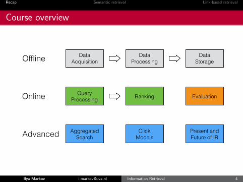
Course overview

Data Acquisition

Data Processing

Data Storage

EvaluationRankingQuery Processing

Aggregated Search

Click Models

Present and Future of IR

Offline

Online

Advanced



Query processing

Data Acquisition

Data Processing

Data Storage


Aggregated Search

Click Models


Offline

Online

Advanced



Query processing

Spell checking

Query expansion

Query suggestion

Query auto-completion



Ranking methods

Data Acquisition

Data Processing

Data Storage


Aggregated Search

Click Models


Offline

Online

Advanced



Ranking methods

1 Content-based

Term-basedSemantic

2 Link-based (web search)

3 Learning to rank



Term-based retrieval

Vector space model

Probabilistic retrieval

Language modeling



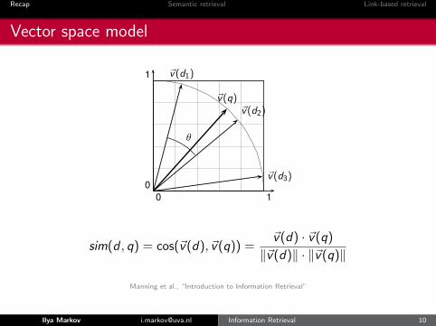
Vector space model

0 10

1

v⃗(q)

v⃗(d1)

v⃗(d2)

v⃗(d3)

θ

sim(d , q) = cos(~v(d), ~v(q)) =~v(d) · ~v(q)

‖~v(d)‖ · ‖~v(q)‖

Manning et al., “Introduction to Information Retrieval”



Probabilistic retrieval

BM25d =∑

t∈qlog

[N

df (t)

]· (k1 + 1) · tf (t, d)

k1 ·[(1− b) + b · dl(d)

dlave

]+ tf (t, d)



Language modeling

Online edition (c)�2009 Cambridge UP

12.1 Language models 239

Model M1 Model M2the 0.2 the 0.15a 0.1 a 0.12frog 0.01 frog 0.0002toad 0.01 toad 0.0001said 0.03 said 0.03likes 0.02 likes 0.04that 0.04 that 0.04dog 0.005 dog 0.01cat 0.003 cat 0.015monkey 0.001 monkey 0.002. . . . . . . . . . . .

! Figure 12.3 Partial specification of two unigram language models.

✎ Example 12.1: To find the probability of a word sequence, we just multiply theprobabilities which the model gives to each word in the sequence, together with theprobability of continuing or stopping after producing each word. For example,

P(frog said that toad likes frog) = (0.01× 0.03× 0.04× 0.01× 0.02× 0.01)(12.2)×(0.8× 0.8× 0.8× 0.8× 0.8× 0.8× 0.2)

≈ 0.000000000001573

As you can see, the probability of a particular string/document, is usually a verysmall number! Here we stopped after generating frog the second time. The first line ofnumbers are the term emission probabilities, and the second line gives the probabil-ity of continuing or stopping after generating each word. An explicit stop probabilityis needed for a finite automaton to be a well-formed language model according toEquation (12.1). Nevertheless, most of the time, we will omit to include STOP and(1− STOP) probabilities (as do most other authors). To compare two models for adata set, we can calculate their likelihood ratio, which results from simply dividing theLIKELIHOOD RATIOprobability of the data according to one model by the probability of the data accord-ing to the other model. Providing that the stop probability is fixed, its inclusion willnot alter the likelihood ratio that results from comparing the likelihood of two lan-guage models generating a string. Hence, it will not alter the ranking of documents.2Nevertheless, formally, the numbers will no longer truly be probabilities, but onlyproportional to probabilities. See Exercise 12.4.

✎ Example 12.2: Suppose, now, that we have two language models M1 and M2,shown partially in Figure 12.3. Each gives a probability estimate to a sequence of

2. In the IR context that we are leading up to, taking the stop probability to be fixed acrossmodels seems reasonable. This is because we are generating queries, and the length distributionof queries is fixed and independent of the document from which we are generating the languagemodel.




Ranking methods

Data Acquisition

Data Processing

Data Storage


Aggregated Search

Click Models


Offline

Online

Advanced



Ranking methods

1 Content-based

Term-basedSemantic


3 Learning to rank



Outline

1 Recap

2 Semantic retrievalLatent semantic indexing/analysisTopic modelingWord embeddingsNeural networksSummary




Problems with term-based retrieval

1 Synonymy

2 Polysemy



Outline




Vector space model

Anthony Julius The Hamlet Othello Macbeth . . .and Caesar Tempest

CleopatraAnthony 1 1 0 0 0 1Brutus 1 1 0 1 0 0Caesar 1 1 0 1 1 1Calpurnia 0 1 0 0 0 0Cleopatra 1 0 0 0 0 0mercy 1 0 1 1 1 1worser 1 0 1 1 1 0. . .




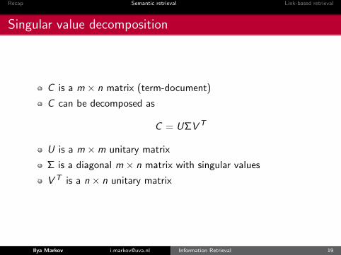
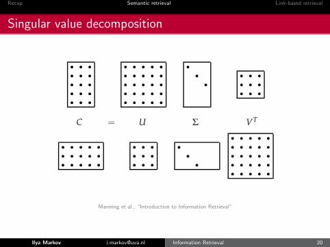
Singular value decomposition

C is a m × n matrix (term-document)

C can be decomposed as

C = UΣV T

U is a m ×m unitary matrix

Σ is a diagonal m × n matrix with singular values

V T is a n × n unitary matrix



Singular value decomposition


18.2 Term-document matrices and singular value decompositions 409

!!!!!

!!!!!

!!!!!

!!!!!

!!!!!

!!!!!

!!!!!

!!!!! ! ! ! !!! !!! !!!

C = U Σ VT

!!! !!! !!! !!! !!! !!! !!! !!! ! ! ! !!!!!

!!!!!

!!!!!

!!!!!

!!!!!

! Figure 18.1 Illustration of the singular-value decomposition. In this schematicillustration of (18.9), we see two cases illustrated. In the top half of the figure, wehave a matrix C for which M > N. The lower half illustrates the case M < N.

as the reduced SVD or truncated SVD and we will encounter it again in Ex-REDUCED SVDTRUNCATED SVD ercise 18.9. Henceforth, our numerical examples and exercises will use this

reduced form.

✎ Example 18.3: We now illustrate the singular-value decomposition of a 4× 2 ma-trix of rank 2; the singular values are Σ11 = 2.236 and Σ22 = 1.

C =

⎛⎜⎜⎝

1 −10 11 0−1 1

⎞⎟⎟⎠ =

⎛⎜⎜⎝

−0.632 0.0000.316 −0.707−0.316 −0.7070.632 0.000

⎞⎟⎟⎠(

2.236 0.0000.000 1.000

)( −0.707 0.707−0.707 −0.707

).(18.11)

As with the matrix decompositions defined in Section 18.1.1, the singu-lar value decomposition of a matrix can be computed by a variety of algo-rithms, many of which have been publicly available software implementa-tions; pointers to these are given in Section 18.5.

? Exercise 18.4

Let

C =

⎛⎝

1 10 11 0

⎞⎠(18.12)

be the term-document incidence matrix for a collection. Compute the co-occurrencematrix CCT. What is the interpretation of the diagonal entries of CCT when C is aterm-document incidence matrix?




Low-rank approximation

C = UΣV T =

min(m,n)∑

i=1

σi ~ui~vTi

≈k∑

i=1

σi ~ui~vTi = UkΣkV

Tk



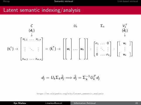
Latent semantic indexing/analysis

C Uk Σk V Tk

(dj) (d̂j)↓ ↓

(tTi )→

x1,1 . . . x1,n

.... . .

...

xm,1 . . . xm,n

= (t̂Ti )→

u1

. . .uk

·

σ1 . . . 0...

. . ....

0 . . . σk

·[

v1

]...[vk

]

dj = UkΣk d̂j =⇒ d̂j = Σ−1k UT

k dj

https://en.wikipedia.org/wiki/Latent_semantic_analysis


https://en.wikipedia.org/wiki/Latent_semantic_analysis


Outline




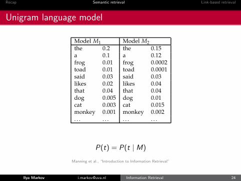
Unigram language model


12.1 Language models 239

Model M1 Model M2the 0.2 the 0.15a 0.1 a 0.12frog 0.01 frog 0.0002toad 0.01 toad 0.0001said 0.03 said 0.03likes 0.02 likes 0.04that 0.04 that 0.04dog 0.005 dog 0.01cat 0.003 cat 0.015monkey 0.001 monkey 0.002. . . . . . . . . . . .

! Figure 12.3 Partial specification of two unigram language models.

✎ Example 12.1: To find the probability of a word sequence, we just multiply theprobabilities which the model gives to each word in the sequence, together with theprobability of continuing or stopping after producing each word. For example,

P(frog said that toad likes frog) = (0.01× 0.03× 0.04× 0.01× 0.02× 0.01)(12.2)×(0.8× 0.8× 0.8× 0.8× 0.8× 0.8× 0.2)

≈ 0.000000000001573

As you can see, the probability of a particular string/document, is usually a verysmall number! Here we stopped after generating frog the second time. The first line ofnumbers are the term emission probabilities, and the second line gives the probabil-ity of continuing or stopping after generating each word. An explicit stop probabilityis needed for a finite automaton to be a well-formed language model according toEquation (12.1). Nevertheless, most of the time, we will omit to include STOP and(1− STOP) probabilities (as do most other authors). To compare two models for adata set, we can calculate their likelihood ratio, which results from simply dividing theLIKELIHOOD RATIOprobability of the data according to one model by the probability of the data accord-ing to the other model. Providing that the stop probability is fixed, its inclusion willnot alter the likelihood ratio that results from comparing the likelihood of two lan-guage models generating a string. Hence, it will not alter the ranking of documents.2Nevertheless, formally, the numbers will no longer truly be probabilities, but onlyproportional to probabilities. See Exercise 12.4.

✎ Example 12.2: Suppose, now, that we have two language models M1 and M2,shown partially in Figure 12.3. Each gives a probability estimate to a sequence of

2. In the IR context that we are leading up to, taking the stop probability to be fixed acrossmodels seems reasonable. This is because we are generating queries, and the length distributionof queries is fixed and independent of the document from which we are generating the languagemodel.

P(t) = P(t | M)




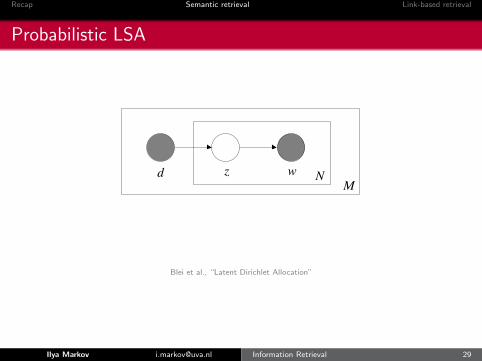
Unigram language modelBLEI, NG, AND JORDAN

wM

N

(a) unigram

z wM

N

(b) mixture of unigrams

z wM

Nd

(c) pLSI/aspect model

Figure 3: Graphical model representation of different models of discrete data.

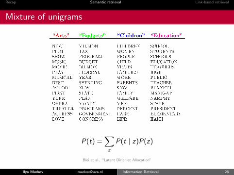
4.2 Mixture of unigrams

If we augment the unigram model with a discrete random topic variable z (Figure 3b), we obtain amixture of unigrams model (Nigam et al., 2000). Under this mixture model, each document is gen-erated by first choosing a topic z and then generating N words independently from the conditionalmultinomial p(w |z). The probability of a document is:

p(w) =∑zp(z)

N

∏n=1

p(wn |z).

When estimated from a corpus, the word distributions can be viewed as representations of topicsunder the assumption that each document exhibits exactly one topic. As the empirical results inSection 7 illustrate, this assumption is often too limiting to effectively model a large collection ofdocuments.

In contrast, the LDA model allows documents to exhibit multiple topics to different degrees.This is achieved at a cost of just one additional parameter: there are k� 1 parameters associatedwith p(z) in the mixture of unigrams, versus the k parameters associated with p(θ |α) in LDA.

4.3 Probabilistic latent semantic indexing

Probabilistic latent semantic indexing (pLSI) is another widely used document model (Hofmann,1999). The pLSI model, illustrated in Figure 3c, posits that a document label d and a word wn are

1000

Blei et al., “Latent Dirichlet Allocation”



Mixture of unigrams

LATENT DIRICHLET ALLOCATION

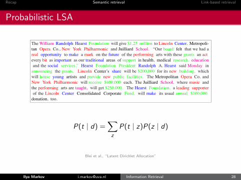
TheWilliam Randolph Hearst Foundation will give $1.25 million to Lincoln Center, Metropoli-tan Opera Co., New York Philharmonic and Juilliard School. “Our board felt that we had areal opportunity to make a mark on the future of the performing arts with these grants an actevery bit as important as our traditional areas of support in health, medical research, educationand the social services,” Hearst Foundation President Randolph A. Hearst said Monday inannouncing the grants. Lincoln Center’s share will be $200,000 for its new building, whichwill house young artists and provide new public facilities. The Metropolitan Opera Co. andNew York Philharmonic will receive $400,000 each. The Juilliard School, where music andthe performing arts are taught, will get $250,000. The Hearst Foundation, a leading supporterof the Lincoln Center Consolidated Corporate Fund, will make its usual annual $100,000donation, too.

Figure 8: An example article from the AP corpus. Each color codes a different factor from whichthe word is putatively generated.

1009

P(t) =∑

z

P(t | z)P(z)




Mixture of unigrams

BLEI, NG, AND JORDAN

wM

N

(a) unigram

z wM

N


z wM

Nd





p(w) =∑zp(z)

N

∏n=1

p(wn |z).





1000




Probabilistic LSA

LATENT DIRICHLET ALLOCATION

TheWilliam Randolph Hearst Foundation will give $1.25 million to Lincoln Center, Metropoli-tan Opera Co., New York Philharmonic and Juilliard School. “Our board felt that we had areal opportunity to make a mark on the future of the performing arts with these grants an actevery bit as important as our traditional areas of support in health, medical research, educationand the social services,” Hearst Foundation President Randolph A. Hearst said Monday inannouncing the grants. Lincoln Center’s share will be $200,000 for its new building, whichwill house young artists and provide new public facilities. The Metropolitan Opera Co. andNew York Philharmonic will receive $400,000 each. The Juilliard School, where music andthe performing arts are taught, will get $250,000. The Hearst Foundation, a leading supporterof the Lincoln Center Consolidated Corporate Fund, will make its usual annual $100,000donation, too.

Figure 8: An example article from the AP corpus. Each color codes a different factor from whichthe word is putatively generated.

1009

P(t | d) =∑

z

P(t | z)P(z | d)




Probabilistic LSA

BLEI, NG, AND JORDAN

wM

N

(a) unigram

z wM

N


z wM

Nd





p(w) =∑zp(z)

N

∏n=1

p(wn |z).





1000




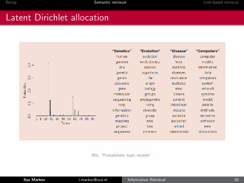
Latent Dirichlet allocation

Blei, “Probabilistic topic models”



Latent Dirichlet allocation

P(t | d) =K∑

z=1

P(t | z , φ)P(z | θ, d)

https://en.wikipedia.org/wiki/Latent_Dirichlet_allocation


https://en.wikipedia.org/wiki/Latent_Dirichlet_allocation


Outline




Word2vec

w(t-2)

w(t+1)

w(t-1)

w(t+2)

w(t)

SUM

INPUT PROJECTION OUTPUT

w(t)


w(t-2)

w(t-1)

w(t+1)

w(t+2)

CBOW Skip-gram

Figure 1: New model architectures. The CBOW architecture predicts the current word based on thecontext, and the Skip-gram predicts surrounding words given the current word.

R words from the future of the current word as correct labels. This will require us to do R ⇥ 2word classifications, with the current word as input, and each of the R + R words as output. In thefollowing experiments, we use C = 10.

4 Results

To compare the quality of different versions of word vectors, previous papers typically use a tableshowing example words and their most similar words, and understand them intuitively. Althoughit is easy to show that word France is similar to Italy and perhaps some other countries, it is muchmore challenging when subjecting those vectors in a more complex similarity task, as follows. Wefollow previous observation that there can be many different types of similarities between words, forexample, word big is similar to bigger in the same sense that small is similar to smaller. Exampleof another type of relationship can be word pairs big - biggest and small - smallest [20]. We furtherdenote two pairs of words with the same relationship as a question, as we can ask: ”What is theword that is similar to small in the same sense as biggest is similar to big?”

Somewhat surprisingly, these questions can be answered by performing simple algebraic operationswith the vector representation of words. To find a word that is similar to small in the same sense asbiggest is similar to big, we can simply compute vector X = vector(”biggest”)�vector(”big”)+vector(”small”). Then, we search in the vector space for the word closest to X measured by cosinedistance, and use it as the answer to the question (we discard the input question words during thissearch). When the word vectors are well trained, it is possible to find the correct answer (wordsmallest) using this method.

Finally, we found that when we train high dimensional word vectors on a large amount of data, theresulting vectors can be used to answer very subtle semantic relationships between words, such asa city and the country it belongs to, e.g. France is to Paris as Germany is to Berlin. Word vectorswith such semantic relationships could be used to improve many existing NLP applications, suchas machine translation, information retrieval and question answering systems, and may enable otherfuture applications yet to be invented.

5

w(t-2)

w(t+1)

w(t-1)

w(t+2)

w(t)

SUM


w(t)


w(t-2)

w(t-1)

w(t+1)

w(t+2)

CBOW Skip-gram

Figure 1: New model architectures. The CBOW architecture predicts the current word based on thecontext, and the Skip-gram predicts surrounding words given the current word.

R words from the future of the current word as correct labels. This will require us to do R ⇥ 2word classifications, with the current word as input, and each of the R + R words as output. In thefollowing experiments, we use C = 10.

4 Results

To compare the quality of different versions of word vectors, previous papers typically use a tableshowing example words and their most similar words, and understand them intuitively. Althoughit is easy to show that word France is similar to Italy and perhaps some other countries, it is muchmore challenging when subjecting those vectors in a more complex similarity task, as follows. Wefollow previous observation that there can be many different types of similarities between words, forexample, word big is similar to bigger in the same sense that small is similar to smaller. Exampleof another type of relationship can be word pairs big - biggest and small - smallest [20]. We furtherdenote two pairs of words with the same relationship as a question, as we can ask: ”What is theword that is similar to small in the same sense as biggest is similar to big?”

Somewhat surprisingly, these questions can be answered by performing simple algebraic operationswith the vector representation of words. To find a word that is similar to small in the same sense asbiggest is similar to big, we can simply compute vector X = vector(”biggest”)�vector(”big”)+vector(”small”). Then, we search in the vector space for the word closest to X measured by cosinedistance, and use it as the answer to the question (we discard the input question words during thissearch). When the word vectors are well trained, it is possible to find the correct answer (wordsmallest) using this method.

Finally, we found that when we train high dimensional word vectors on a large amount of data, theresulting vectors can be used to answer very subtle semantic relationships between words, such asa city and the country it belongs to, e.g. France is to Paris as Germany is to Berlin. Word vectorswith such semantic relationships could be used to improve many existing NLP applications, suchas machine translation, information retrieval and question answering systems, and may enable otherfuture applications yet to be invented.

5

Mikolov et al., “Efficient Estimation of Word Representations in Vector Space”



Word2vec algorithm

1 Choose the length of embeddings

2 Initialize embeddings randomly

3 Update embeddings using gradient descent by optimizingCBOW or Skip-gram



Word2vec example

-2

-1.5

-1

-0.5

0

0.5

1

1.5

2

-2 -1.5 -1 -0.5 0 0.5 1 1.5 2

Country and Capital Vectors Projected by PCAChina

Japan

France

Russia

Germany

Italy

SpainGreece

Turkey

Beijing

Paris

Tokyo

Poland

Moscow

Portugal

Berlin

RomeAthens

Madrid

Ankara

Warsaw

Lisbon

Figure 2: Two-dimensional PCA projection of the 1000-dimensional Skip-gram vectors of countries and theircapital cities. The figure illustrates ability of the model to automatically organize concepts and learn implicitlythe relationships between them, as during the training we did not provide any supervised information aboutwhat a capital city means.

which is used to replace every log P (wO|wI) term in the Skip-gram objective. Thus the task is todistinguish the target word wO from draws from the noise distribution Pn(w) using logistic regres-sion, where there are k negative samples for each data sample. Our experiments indicate that valuesof k in the range 5–20 are useful for small training datasets, while for large datasets the k can be assmall as 2–5. The main difference between the Negative sampling and NCE is that NCE needs bothsamples and the numerical probabilities of the noise distribution, while Negative sampling uses onlysamples. And while NCE approximately maximizes the log probability of the softmax, this propertyis not important for our application.

Both NCE and NEG have the noise distributionPn(w) as a free parameter. We investigated a numberof choices for Pn(w) and found that the unigram distribution U(w) raised to the 3/4rd power (i.e.,U(w)3/4/Z) outperformed significantly the unigram and the uniform distributions, for both NCEand NEG on every task we tried including language modeling (not reported here).

2.3 Subsampling of Frequent Words

In very large corpora, the most frequent words can easily occur hundreds of millions of times (e.g.,“in”, “the”, and “a”). Such words usually provide less information value than the rare words. Forexample, while the Skip-gram model benefits from observing the co-occurrences of “France” and“Paris”, it benefits much less from observing the frequent co-occurrences of “France” and “the”, asnearly every word co-occurs frequently within a sentence with “the”. This idea can also be appliedin the opposite direction; the vector representations of frequent words do not change significantlyafter training on several million examples.

To counter the imbalance between the rare and frequent words, we used a simple subsampling ap-proach: each word wi in the training set is discarded with probability computed by the formula

P (wi) = 1 −!

t

f(wi)(5)

4

Mikolov et al., “Distributed Representations of Words and Phrases and their Compositionality”



Word2vec for retrieval

Average word embeddings (centroids) for queries anddocuments

Cosine similarity

Works best for short documents



Outline




Deep structured semantic model

DNN model is used for Web document ranking as follows: 1) to map term vectors to their corresponding semantic concept vectors; 2) to compute the relevance score between a document and a query as cosine similarity of their corresponding semantic concept vectors; rf. Eq. (3) to (5).

More formally, if we denote ! as the input term vector, " as the output vector, #

!, % & 1,… , ) * 1, as the intermediate hidden

layers, +! as the i-th weight matrix, and ,

! as the %-th bias term,

we have

#"& +

"!

#!& -.+

!#!#"

/ ,!0, % & 2, … ,) * 1

" & -.+$#$#"

/ ,$0

(3)

where we use the 2345 as the activation function at the output layer and the hidden layers #

!, % & 2, … , ) * 1:

-.!0 &1 * 7

#%&

1 / 7#%& (4)

The semantic relevance score between a query 8 and a document 9 is then measured as:

:.8, 90 & cosineA"', "

(B &

"'

)"(

‖"'‖‖"

(‖

(5)

where "'

and "(

are the concept vectors of the query and the document, respectively. In Web search, given the query, the documents are sorted by their semantic relevance scores.

Conventionally, the size of the term vector, which can be viewed as the raw bag-of-words features in IR, is identical to that of the vocabulary that is used for indexing the Web document collection. The vocabulary size is usually very large in real-world Web search tasks. Therefore, when using term vector as the input, the size of the input layer of the neural network would be unmanageable for inference and model training. To address this problem, we have developed a method called “word hashing” for the first layer of the DNN, as indicated in the lower portion of Figure 1. This layer consists of only linear hidden units in which the weight matrix of a very large size is not learned. In the following section, we describe the word hashing method in detail.

3.2 Word Hashing The word hashing method described here aims to reduce the dimensionality of the bag-of-words term vectors. It is based on letter n-gram, and is a new method developed especially for our task. Given a word (e.g. good), we first add word starting and ending marks to the word (e.g. #good#). Then, we break the word into letter n-grams (e.g. letter trigrams: #go, goo, ood, od#). Finally, the word is represented using a vector of letter n-grams.

One problem of this method is collision, i.e., two different words could have the same letter n-gram vector representation. Table 1 shows some statistics of word hashing on two vocabularies. Compared with the original size of the one-hot vector, word hashing allows us to represent a query or a document using a vector with much lower dimensionality. Take the 40K-word vocabulary as an example. Each word can be represented by a 10,306-dimentional vector using letter trigrams, giving a four-fold dimensionality reduction with few collisions. The reduction of dimensionality is even more significant when the technique is applied to a larger vocabulary. As shown in Table 1, each word in the 500K-word vocabulary can be represented by a 30,621 dimensional vector using letter trigrams, a reduction of 16-fold in dimensionality with a negligible collision rate of 0.0044% (22/500,000).

While the number of English words can be unlimited, the number of letter n-grams in English (or other similar languages) is often limited. Moreover, word hashing is able to map the morphological variations of the same word to the points that are close to each other in the letter n-gram space. More importantly, while a word unseen in the training set always causes difficulties in word-based representations, it is not the case where the letter n-gram based representation is used. The only risk is the minor representation collision as quantified in Table 1. Thus, letter n-gram based word hashing is robust to the out-of-vocabulary problem, allowing us to scale up the DNN solution to the Web search tasks where extremely large vocabularies are desirable. We will demonstrate the benefit of the technique in Section 4.

In our implementation, the letter n-gram based word hashing can be viewed as a fixed (i.e., non-adaptive) linear transformation,

Figure 1: Illustration of the DSSM. It uses a DNN to map high-dimensional sparse text features into low-dimensional dense features in a semantic space. The first hidden layer, with 30k units, accomplishes word hashing. The word-hashed features are then projected through multiple layers of non-linear projections. The final layer’s neural activities in this DNN form the feature in the semantic space.

l1 = W1x

li = f (Wi li−1 + bi )

y = f (WnlN−1 + bN)

Huang et al. “Learning Deep Structured Semantic Models for Web Search using Clickthrough Data”



Experimental comparisonlayers from one to three raises the NDCG scores by 0.4-0.5 point which are statistically significant, while there is no significant difference between linear and non-linear models if both are one-layer shallow models (Row 10 vs. Row 11).

# Models NDCG@1 NDCG@3 NDCG@10 1 TF-IDF 0.319 0.382 0.462 2 BM25 0.308 0.373 0.455 3 WTM 0.332 0.400 0.478 4 LSA 0.298 0.372 0.455 5 PLSA 0.295 0.371 0.456 6 DAE 0.310 0.377 0.459 7 BLTM-PR 0.337 0.403 0.480 8 DPM 0.329 0.401 0.479 9 DNN 0.342 0.410 0.486

10 L-WH linear 0.357 0.422 0.495 11 L-WH non-linear 0.357 0.421 0.494 12 L-WH DNN 0.362 0.425 0.498 Table 2: Comparative results with the previous state of the art approaches and various settings of DSSM.

5. CONCLUSIONS We present and evaluate a series of new latent semantic models, notably those with deep architectures which we call the DSSM. The main contribution lies in our significant extension of the previous latent semantic models (e.g., LSA) in three key aspects. First, we make use of the clickthrough data to optimize the parameters of all versions of the models by directly targeting the goal of document ranking. Second, inspired by the deep learning framework recently shown to be highly successful in speech recognition [5][13][14][16][18], we extend the linear semantic models to their nonlinear counterparts using multiple hidden-representation layers. The deep architectures adopted have further enhanced the modeling capacity so that more sophisticated semantic structures in queries and documents can be captured and represented. Third, we use a letter n-gram based word hashing technique that proves instrumental in scaling up the training of the deep models so that very large vocabularies can be used in realistic web search. In our experiments, we show that the new techniques pertaining to each of the above three aspects lead to significant performance improvement on the document ranking task. A combination of all three sets of new techniques has led to a new state-of-the-art semantic model that beats all the previously developed competing models with a significant margin.

REFERENCES [1] Bengio, Y., 2009. “Learning deep architectures for AI.”

Foundumental Trends Machine Learning, vol. 2. [2] Blei, D. M., Ng, A. Y., and Jordan, M. J. 2003. “Latent

Dirichlet allocation.” In JMLR, vol. 3. [3] Burges, C., Shaked, T., Renshaw, E., Lazier, A., Deeds, M.,

Hamilton, and Hullender, G. 2005. “Learning to rank using gradient descent.” In ICML.

[4] Collobert, R., Weston, J., Bottou, L., Karlen, M., Kavukcuoglu, K., and Kuksa, P., 2011. “Natural language processing (almost) from scratch.” in JMLR, vol. 12.

[5] Dahl, G., Yu, D., Deng, L., and Acero, A., 2012. “Context-dependent pre-trained deep neural networks for large vocabulary speech recognition.” in IEEE Transactions on Audio, Speech, and Language Processing.

[6] Deerwester, S., Dumais, S. T., Furnas, G. W., Landauer, T., and Harshman, R. 1990. “Indexing by latent semantic analysis.” J. American Society for Information Science, 41(6): 391-407

[7] Deng, L., He, X., and Gao, J., 2013. "Deep stacking networks for information retrieval." In ICASSP

[8] Dumais, S. T., Letsche, T. A., Littman, M. L., and Landauer, T. K. 1997. “Automatic cross-linguistic information retrieval using latent semantic indexing.” In AAAI-97 Spring Sympo-sium Series: Cross-Language Text and Speech Retrieval.

[9] Gao, J., He, X., and Nie, J-Y. 2010. “Clickthrough-based translation models for web search: from word models to phrase models.” In CIKM.

[10] Gao, J., Toutanova, K., Yih., W-T. 2011. “Clickthrough-based latent semantic models for web search.” In SIGIR.

[11] Gao, J., Yuan, W., Li, X., Deng, K., and Nie, J-Y. 2009. “Smoothing clickthrough data for web search ranking.” In SIGIR.

[12] He, X., Deng, L., and Chou, W., 2008. “Discriminative learning in sequential pattern recognition,” Sept. IEEE Sig. Proc. Mag.

[13] Heck, L., Konig, Y., Sonmez, M. K., and Weintraub, M. 2000. “Robustness to telephone handset distortion in speaker recognition by discriminative feature design.” In Speech Communication.

[14] Hinton, G., Deng, L., Yu, D., Dahl, G., Mohamed, A., Jaitly, N., Senior, A., Vanhoucke, V., Nguyen, P., Sainath, T., and Kingsbury, B., 2012. “Deep neural networks for acoustic modeling in speech recognition,” IEEE Sig. Proc. Mag.

[15] Hofmann, T. 1999. “Probabilistic latent semantic indexing.” In SIGIR.

[16] Hutchinson, B., Deng, L., and Yu, D., 2013. “Tensor deep stacking networks.” In IEEE T-PAMI, vol. 35.

[17] Jarvelin, K. and Kekalainen, J. 2000. “IR evaluation methods for retrieving highly relevant documents.” In SIGIR.

[18] Konig, Y., Heck, L., Weintraub, M., and Sonmez, M. K. 1998. “Nonlinear discriminant feature extraction for robust text-independent speaker recognition.” in RLA2C.

[19] Mesnil, G., He, X., Deng, L., and Bengio, Y., 2013. “Investigation of recurrent-neural-network architectures and learning methods for spoken language understanding.” In Interspeech.

[20] Montavon, G., Orr, G., Müller, K., 2012. Neural Networks: Tricks of the Trade (Second edition). Springer.

[21] Platt, J., Toutanova, K., and Yih, W. 2010. “Translingual doc-ument representations from discriminative projections.” In EMNLP.

[22] Salakhutdinov R., and Hinton, G., 2007 “Semantic hashing.” in Proc. SIGIR Workshop Information Retrieval and Applications of Graphical Models.

[23] Socher, R., Huval, B., Manning, C., Ng, A., 2012. “Semantic compositionality through recursive matrix-vector spaces.” In EMNLP.

[24] Svore, K., and Burges, C. 2009. “A machine learning approach for improved BM25 retrieval.” In CIKM.

[25] Tur, G., Deng, L., Hakkani-Tur, D., and He, X., 2012. “Towards deeper understanding deep convex networks for semantic utterance classification.” In ICASSP.

[26] Yih, W., Toutanova, K., Platt, J., and Meek, C. 2011. “Learning discriminative projections for text similarity measures.” In CoNLL.

DNN – no semantic hashing

L-WH linear – semantic hashing, NO non-linear activation functions

L-WH non-linear – semantic hashing, non-linear activation functions

L-WH DNN – full network

Huang et al. “Learning Deep Structured Semantic Models for Web Search using Clickthrough Data”



Outline




Semantic retrieval summary

Latent semantic indexing/analysis

Topic modeling (pLSA, LDA)

Words embeddings (word2vec)

Neural networks (DSSM)



Materials

Manning et al., Chapter 18

Blei et al.Latent Dirichlet AllocationJournal of Machine Learning Research, 2003

Mikolov et al.Distributed Representations of Words and Phrases andtheir CompositionalityAdvances in neural information processing systems, 2013

Huang et al.Learning Deep Structured Semantic Models for WebSearch using Clickthrough DataProceedings of CIKM, 2013



Ranking methods

1 Content-based

Term-basedSemantic


3 Learning to rank



Outline

1 Recap


3 Link-based retrievalPageRankHITSSummary



Linear algebra

C – square M ×M matrix

~x – M-dimensional vector

C~x = λ~x

λ – eigenvalue~x – right eigenvector

~yTC = λ~yT

~y – right eigenvector

Principal eigenvector – eigenvector corresponding to thelargest eigenvalue

There are many efficient algorithms to compute eigenvaluesand eigenvectors



Outline




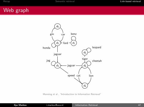
Web graph

Example web graph

d0

d2 d1

d5

d3 d6

d4

car benz

ford

gm

honda

jaguar

jag

cat

leopard

tiger

jaguar

lion

cheetah

speed

PageRank

d0 0.05d1 0.04d2 0.11d3 0.25d4 0.21d5 0.04d6 0.31

PageRank(d2)<PageRank(d6):why?

a h

d0 0.10 0.03d1 0.01 0.04d2 0.12 0.33d3 0.47 0.18d 0.16 0.04

23 / 80Manning et al., “Introduction to Information Retrieval”



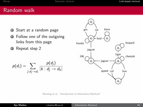
Random walk

1 Start at a random page

2 Follow one of the outgoinglinks from this page

3 Repeat step 2

p(di ) =∑

j :dj→di

p(dj)

|k : dj → dk |

Example web graph

d0

d2 d1

d5

d3 d6

d4

car benz

ford

gm

honda

jaguar

jag

cat

leopard

tiger

jaguar

lion

cheetah

speed

PageRank

d0 0.05d1 0.04d2 0.11d3 0.25d4 0.21d5 0.04d6 0.31


a h

d0 0.10 0.03d1 0.01 0.04d2 0.12 0.33d3 0.47 0.18d 0.16 0.04

23 / 80




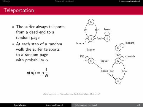
Teleportation

The surfer always teleportsfrom a dead end to arandom page

At each step of a randomwalk the surfer teleportsto a random pagewith probability α

p(di ) = α1

N

Example web graph

d0

d2 d1

d5

d3 d6

d4

car benz

ford

gm

honda

jaguar

jag

cat

leopard

tiger

jaguar

lion

cheetah

speed

PageRank

d0 0.05d1 0.04d2 0.11d3 0.25d4 0.21d5 0.04d6 0.31


a h

d0 0.10 0.03d1 0.01 0.04d2 0.12 0.33d3 0.47 0.18d 0.16 0.04

23 / 80




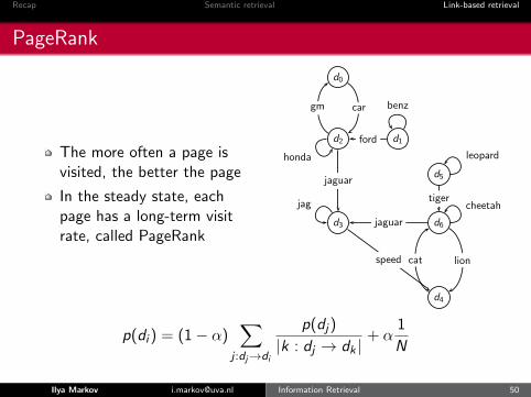
PageRank

The more often a page isvisited, the better the page

In the steady state, eachpage has a long-term visitrate, called PageRank

Example web graph

d0

d2 d1

d5

d3 d6

d4

car benz

ford

gm

honda

jaguar

jag

cat

leopard

tiger

jaguar

lion

cheetah

speed

PageRank

d0 0.05d1 0.04d2 0.11d3 0.25d4 0.21d5 0.04d6 0.31


a h

d0 0.10 0.03d1 0.01 0.04d2 0.12 0.33d3 0.47 0.18d 0.16 0.04

23 / 80

p(di ) = (1− α)∑

j :dj→di

p(dj)

|k : dj → dk |+ α

1

N



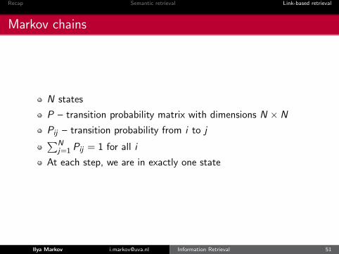
Markov chains

N states

P – transition probability matrix with dimensions N × N

Pij – transition probability from i to j∑N

j=1 Pij = 1 for all i

At each step, we are in exactly one state



Link matrix

d0 d1 d2 d3 d4 d5 d6

d0 0 0 1 0 0 0 0d1 0 1 1 0 0 0 0d2 1 0 1 1 0 0 0d3 0 0 0 1 1 0 0d4 0 0 0 0 0 0 1d5 0 0 0 0 0 1 1d6 0 0 0 1 1 0 1




Transition probability matrix P

d0 d1 d2 d3 d4 d5 d6

d0 0.00 0.00 1.00 0.00 0.00 0.00 0.00d1 0.00 0.50 0.50 0.00 0.00 0.00 0.00d2 0.33 0.00 0.33 0.33 0.00 0.00 0.00d3 0.00 0.00 0.00 0.50 0.50 0.00 0.00d4 0.00 0.00 0.00 0.00 0.00 0.00 1.00d5 0.00 0.00 0.00 0.00 0.00 0.50 0.50d6 0.00 0.00 0.00 0.33 0.33 0.00 0.33




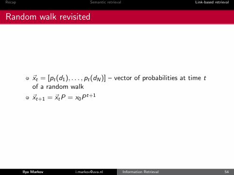
Random walk revisited

~xt = [pt(d1), . . . , pt(dN)] – vector of probabilities at time tof a random walk

~xt+1 = ~xtP = x0Pt+1



Ergodic Markov chains

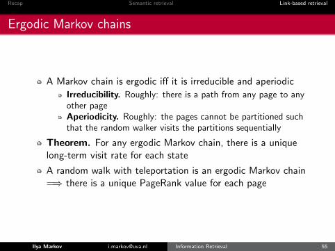
A Markov chain is ergodic iff it is irreducible and aperiodic

Irreducibility. Roughly: there is a path from any page to anyother pageAperiodicity. Roughly: the pages cannot be partitioned suchthat the random walker visits the partitions sequentially

Theorem. For any ergodic Markov chain, there is a uniquelong-term visit rate for each state

A random walk with teleportation is an ergodic Markov chain=⇒ there is a unique PageRank value for each page



PageRank revisited

~π = [PR(d1), . . . ,PR(dN)] – vector of stationary probabilities

1~π = ~πP

λ = 1 – the largest eigenvalue

~π – principal eigenvector



Computing PageRank using power iteration

For any initial distribution vector ~x

For large t

~xPt is very similar to ~xPt+1

~π ≈ ~xPt



Example


468 21 Link analysis

21.2.2 The PageRank computation

How do we compute PageRank values? Recall the definition of a left eigen-vector from Equation 18.2; the left eigenvectors of the transition probabilitymatrix P are N-vectors π⃗ such that

π⃗ P = λπ⃗.(21.2)

The N entries in the principal eigenvector π⃗ are the steady-state proba-bilities of the random walk with teleporting, and thus the PageRank valuesfor the corresponding web pages. We may interpret Equation (21.2) as fol-lows: if π⃗ is the probability distribution of the surfer across the web pages,he remains in the steady-state distribution π⃗. Given that π⃗ is the steady-statedistribution, we have that πP = 1π, so 1 is an eigenvalue of P. Thus if wewere to compute the principal left eigenvector of the matrix P — the one witheigenvalue 1 — we would have computed the PageRank values.

There are many algorithms available for computing left eigenvectors; thereferences at the end of Chapter 18 and the present chapter are a guide tothese. We give here a rather elementary method, sometimes known as poweriteration. If x⃗ is the initial distribution over the states, then the distribution attime t is x⃗Pt. As t grows large, we would expect that the distribution x⃗Pt2

is very similar to the distribution x⃗Pt+1, since for large t we would expectthe Markov chain to attain its steady state. By Theorem 21.1 this is indepen-dent of the initial distribution x⃗. The power iteration method simulates thesurfer’s walk: begin at a state and run the walk for a large number of stepst, keeping track of the visit frequencies for each of the states. After a largenumber of steps t, these frequencies “settle down” so that the variation in thecomputed frequencies is below some predetermined threshold. We declarethese tabulated frequencies to be the PageRank values.

We consider the web graph in Exercise 21.6 with α = 0.5. The transitionprobability matrix of the surfer’s walk with teleportation is then

P =

⎛⎝

1/6 2/3 1/65/12 1/6 5/121/6 2/3 1/6

⎞⎠ .(21.3)

Imagine that the surfer starts in state 1, corresponding to the initial proba-bility distribution vector x⃗0 = (1 0 0). Then, after one step the distributionis

x⃗0P =(

1/6 2/3 1/6)

= x⃗1.(21.4)

2. Note that Pt represents P raised to the tth power, not the transpose of P which is denoted PT.


21.2 PageRank 469

x⃗0 1 0 0x⃗1 1/6 2/3 1/6x⃗2 1/3 1/3 1/3x⃗3 1/4 1/2 1/4x⃗4 7/24 5/12 7/24. . . · · · · · · · · ·x⃗ 5/18 4/9 5/18

! Figure 21.3 The sequence of probability vectors.

After two steps it is

x⃗1P =(

1/6 2/3 1/6)⎛⎝

1/6 2/3 1/65/12 1/6 5/121/6 2/3 1/6

⎞⎠ =

(1/3 1/3 1/3

)= x⃗2.(21.5)

Continuing in this fashion gives a sequence of probability vectors as shownin Figure 21.3.

Continuing for several steps, we see that the distribution converges to thesteady state of x⃗ = (5/18 4/9 5/18). In this simple example, we maydirectly calculate this steady-state probability distribution by observing thesymmetry of the Markov chain: states 1 and 3 are symmetric, as evident fromthe fact that the first and third rows of the transition probability matrix inEquation (21.3) are identical. Postulating, then, that they both have the samesteady-state probability and denoting this probability by p, we know that thesteady-state distribution is of the form π⃗ = (p 1− 2p p). Now, using theidentity π⃗ = π⃗P, we solve a simple linear equation to obtain p = 5/18 andconsequently, π⃗ = (5/18 4/9 5/18).

The PageRank values of pages (and the implicit ordering amongst them)are independent of any query a user might pose; PageRank is thus a query-independent measure of the static quality of each web page (recall such staticquality measures from Section 7.1.4). On the other hand, the relative order-ing of pages should, intuitively, depend on the query being served. For thisreason, search engines use static quality measures such as PageRank as justone of many factors in scoring a web page on a query. Indeed, the relativecontribution of PageRank to the overall score may again be determined bymachine-learned scoring as in Section 15.4.1.




PageRank summary

PageRank is a query-independent indicator of the page quality

PageRank is a stationary state of a random walk withteleportation

A random walk with teleportation is an ergodic Markov chain=⇒ there is a unique PageRank value for each page

PageRank is a principal eigenvector of the transition matrix P=⇒ it can be computed using any algorithm for findingeigenvectors



Outline




Intuition

Hub – a page with a good list of links to pages answering theinformation need

Authority – a page with an answer to the information need

A good hub for a topic links to many authorities for that topic

A good authority for a topic is linked to by many hubs forthat topic



Example Example for hubs and authorities

hubs authorities

www.bestfares.com

www.airlinesquality.com

blogs.usatoday.com/sky

aviationblog.dallasnews.com

www.aa.com

www.delta.com

www.united.com

56 / 80




Computing hub and authority scores

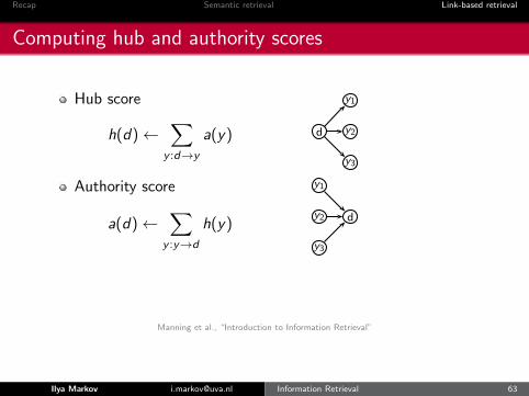
Hub score

h(d)←∑

y :d→y

a(y)

Authority score

a(d)←∑

y :y→d

h(y)

Iterative update

For all d : h(d) =!

d !→y a(y)

d

y1

y2

y3

For all d : a(d) =!

y !→d h(y)

d

y1

y2

y3

Iterate these two steps until convergence

61 / 80

Iterative update

For all d : h(d) =!

d !→y a(y)

d

y1

y2

y3

For all d : a(d) =!

y !→d h(y)

d

y1

y2

y3

Iterate these two steps until convergence

61 / 80




Computing hub and authority scores

A – incidence matrix

Vectorized form of the hub and authority scores

~h← A~a

~a← AT~h

Can be rewritten as

~h← AAT~h

~a← ATA~a

~h and ~a are the eigenvectors of AAT and ATA respectively



Hypertext-induced topic search (HITS)

1 Assemble the target query-dependent subset of web pages

2 Form the graph, induced by their hyperlinks

3 Compute AAT and ATA

4 Compute the principal eigenvectors of AAT and ATA

5 Form the vector of hub scores ~h and authority scores ~a

6 Output the top-scoring hubs and the top-scoring authorities



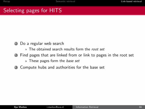
Selecting pages for HITS

1 Do a regular web search

The obtained search results form the root set

2 Find pages that are linked from or link to pages in the root set

These pages form the base set

3 Compute hubs and authorities for the base set



HITS summary

HITS is a query- and link-dependent indicator of the pagequality

Can be computed using any algorithm for finding eigenvectors

Usually, too expensive to be applied at a query time

In practice, usually a good hub is also a good authority

Therefore, the actual difference between PageRank rankingand HITS ranking is not large



Outline




Link-based retrieval summary

PageRank

Query-independentCan be precomputed

HITS

Query-dependentCannot be precomputedIn practice, could be similar to PageRank



Materials

Manning et al., Chapters 21.2–21.3

Croft et al., Chapter 4.5



Ranking methods

1 Content-based

Term-basedSemantic


3 Learning to rank


Информационный поиск, осень 2016: Ранжирование с помощью...

Documents