© 2008 prentice-hall, inc. chapter 7 to accompany quantitative analysis for management, tenth...
TRANSCRIPT
© 2008 Prentice-Hall, Inc.
Chapter 7
To accompanyQuantitative Analysis for Management, Tenth Edition, by Render, Stair, and Hanna Power Point slides created by Jeff Heyl
Linear Programming Models: Graphical and Computer
Methods
© 2009 Prentice-Hall, Inc.
© 2009 Prentice-Hall, Inc. 7 – 2
Introduction
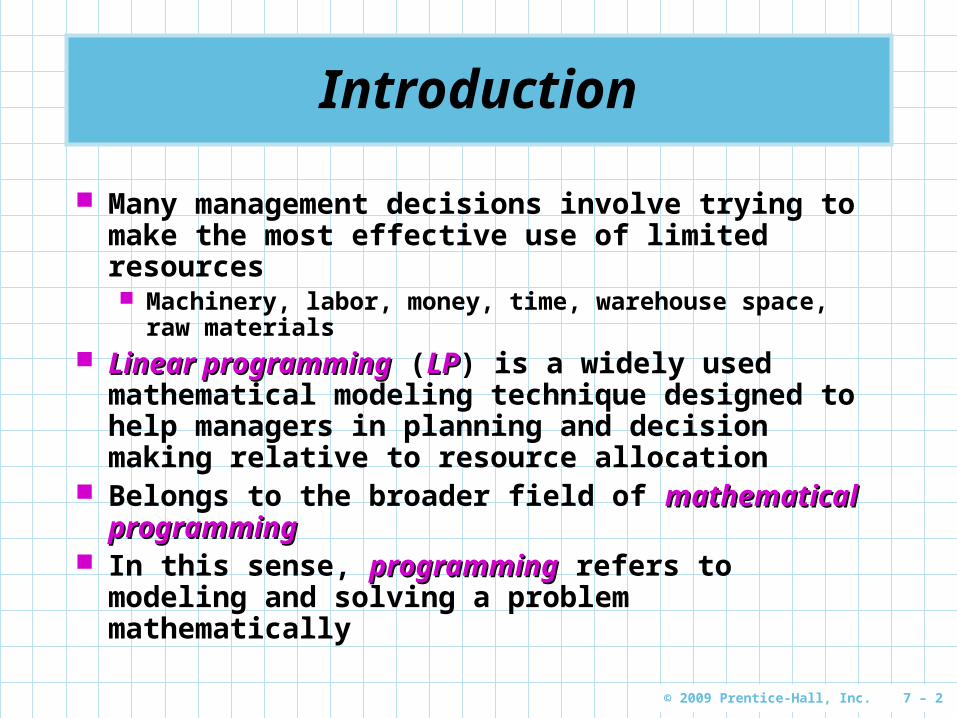
Many management decisions involve trying to make the most effective use of limited resources Machinery, labor, money, time, warehouse space, raw
materials Linear programmingLinear programming (LPLP) is a widely used
mathematical modeling technique designed to help managers in planning and decision making relative to resource allocation
Belongs to the broader field of mathematical mathematical programmingprogramming
In this sense, programmingprogramming refers to modeling and solving a problem mathematically

© 2009 Prentice-Hall, Inc. 7 – 3
Requirements of a Linear Programming Problem
LP has been applied in many areas over the past 50 years
All LP problems have 4 properties in common
1. All problems seek to maximizemaximize or minimizeminimize some quantity (the objective functionobjective function)
2. The presence of restrictions or constraintsconstraints that limit the degree to which we can pursue our objective
3. There must be alternative courses of action to choose from
4. The objective and constraints in problems must be expressed in terms of linearlinear equations or inequalitiesinequalities
© 2009 Prentice-Hall, Inc. 7 – 4
Examples of Successful LP Applications
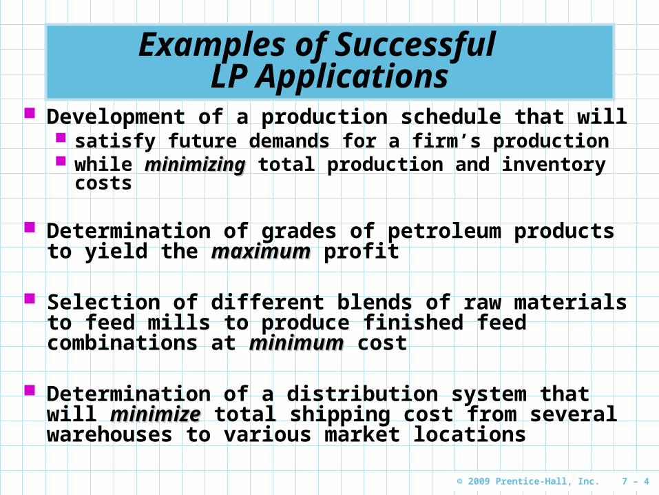
Development of a production schedule that will satisfy future demands for a firm’s production while minimizingminimizing total production and inventory costs
Determination of grades of petroleum products to yield the maximummaximum profit
Selection of different blends of raw materials to feed mills to produce finished feed combinations at minimumminimum cost
Determination of a distribution system that will minimizeminimize total shipping cost from several warehouses to various market locations
© 2009 Prentice-Hall, Inc. 7 – 5
LP Properties and Assumptions
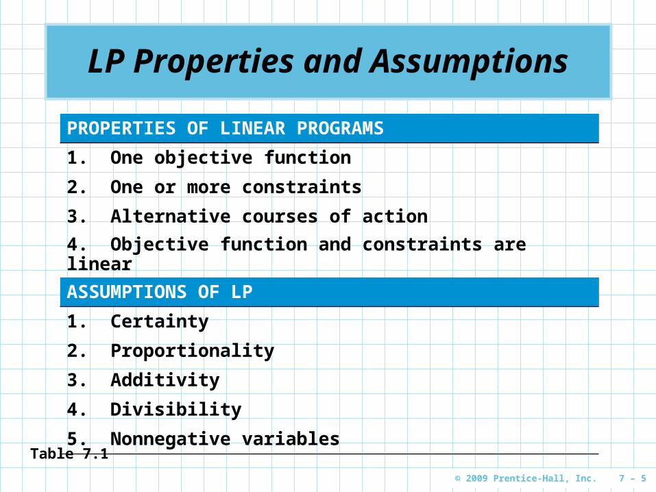
PROPERTIES OF LINEAR PROGRAMS
1. One objective function
2. One or more constraints
3. Alternative courses of action
4. Objective function and constraints are linear
ASSUMPTIONS OF LP
1. Certainty
2. Proportionality
3. Additivity
4. Divisibility
5. Nonnegative variables
Table 7.1
© 2009 Prentice-Hall, Inc. 7 – 6
Basic Assumptions of LP
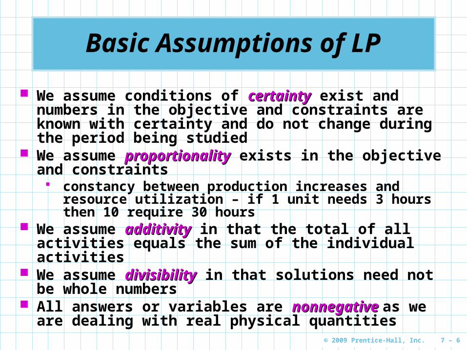
We assume conditions of certaintycertainty exist and numbers in the objective and constraints are known with certainty and do not change during the period being studied
We assume proportionalityproportionality exists in the objective and constraints
constancy between production increases and resource utilization – if 1 unit needs 3 hours then 10 require 30 hours
We assume additivityadditivity in that the total of all activities equals the sum of the individual activities
We assume divisibilitydivisibility in that solutions need not be whole numbers
All answers or variables are nonnegative nonnegative as we are dealing with real physical quantities

© 2009 Prentice-Hall, Inc. 7 – 7
Formulating LP Problems
Formulating a linear program involves developing a mathematical model to represent the managerial problem
The steps in formulating a linear program are1. Completely understand the managerial
problem being faced2. Identify the objective and constraints3. Define the decision variables4. Use the decision variables to write
mathematical expressions for the objective function and the constraints
© 2009 Prentice-Hall, Inc. 7 – 8
Formulating LP Problems
One of the most common LP applications is the product mix problemproduct mix problem
Two or more products are produced using limited resources such as personnel, machines, and raw materials
The profit that the firm seeks to maximize is based on the profit contribution per unit of each product
The company would like to determine how many units of each product it should produce so as to maximize overall profit given its limited resources
© 2009 Prentice-Hall, Inc. 7 – 9
Flair Furniture Company
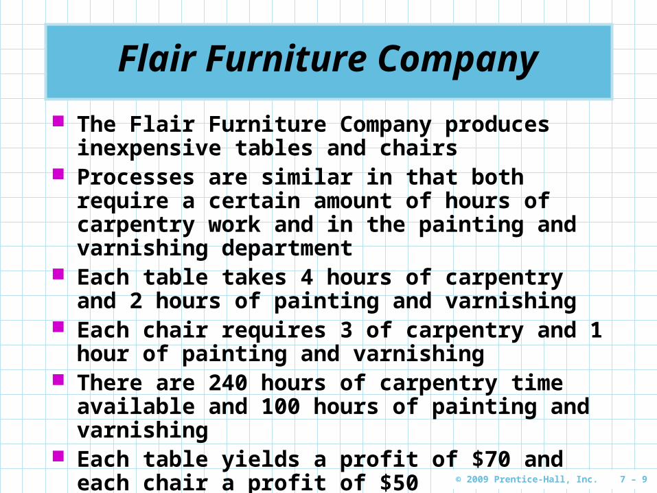
The Flair Furniture Company produces inexpensive tables and chairs
Processes are similar in that both require a certain amount of hours of carpentry work and in the painting and varnishing department
Each table takes 4 hours of carpentry and 2 hours of painting and varnishing
Each chair requires 3 of carpentry and 1 hour of painting and varnishing
There are 240 hours of carpentry time available and 100 hours of painting and varnishing
Each table yields a profit of $70 and each chair a profit of $50
© 2009 Prentice-Hall, Inc. 7 – 10
Flair Furniture Company
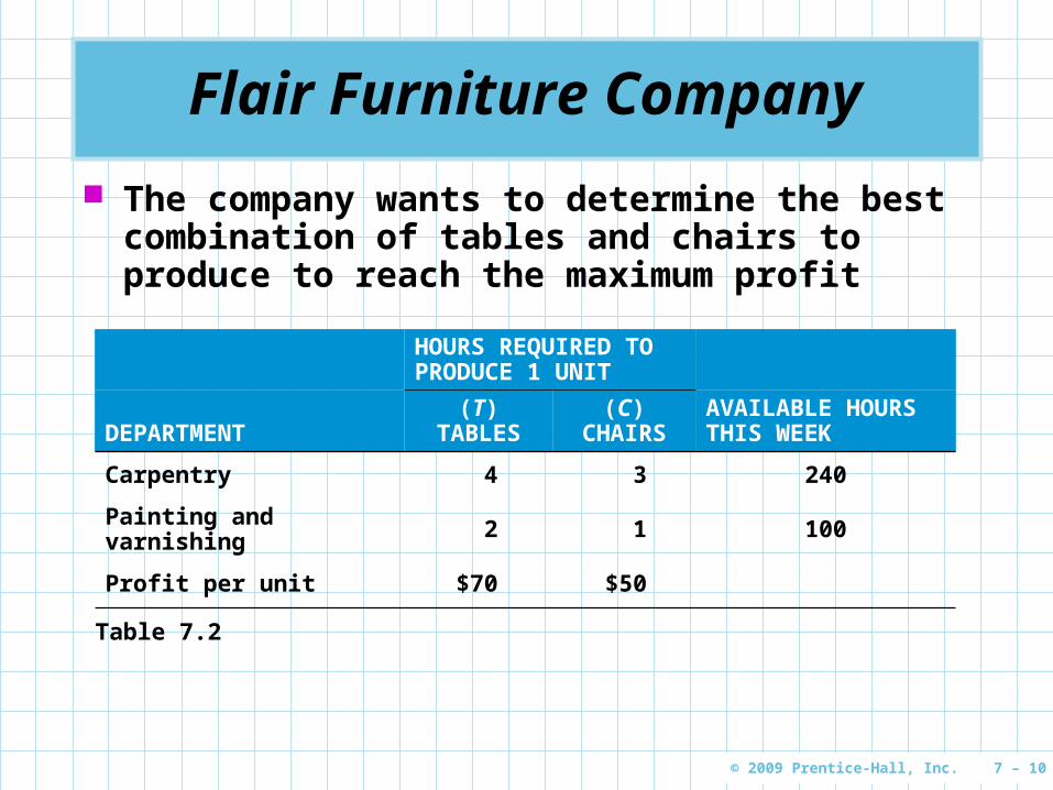
The company wants to determine the best combination of tables and chairs to produce to reach the maximum profit
HOURS REQUIRED TO PRODUCE 1 UNIT
DEPARTMENT(T)
TABLES(C)
CHAIRSAVAILABLE HOURS THIS WEEK
Carpentry 4 3 240
Painting and varnishing 2 1 100
Profit per unit $70 $50
Table 7.2
© 2009 Prentice-Hall, Inc. 7 – 11
Flair Furniture Company
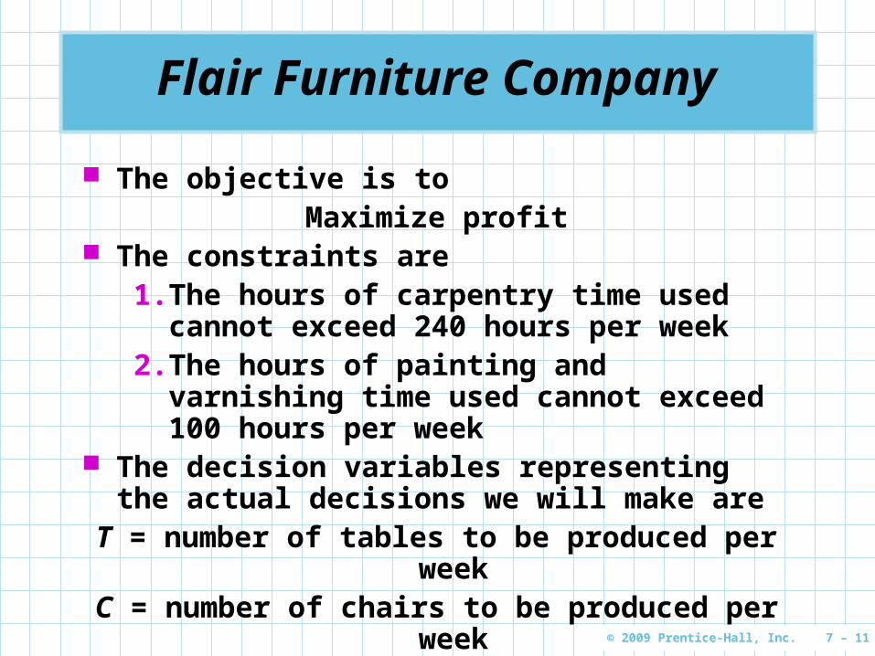
The objective is toMaximize profit
The constraints are1. The hours of carpentry time used cannot
exceed 240 hours per week2. The hours of painting and varnishing time
used cannot exceed 100 hours per week The decision variables representing the actual
decisions we will make areT = number of tables to be produced per weekC = number of chairs to be produced per week

© 2009 Prentice-Hall, Inc. 7 – 12
Flair Furniture Company
We create the LP objective function in terms of T and C
Maximize profit = $70T + $50C Develop mathematical relationships for the two
constraints For carpentry, total time used is
(4 hours per table)(Number of tables produced)+ (3 hours per chair)(Number of chairs
produced) We know that
Carpentry time used ≤ Carpentry time available4T + 3C ≤ 240 (hours of carpentry time)
© 2009 Prentice-Hall, Inc. 7 – 13
Flair Furniture Company
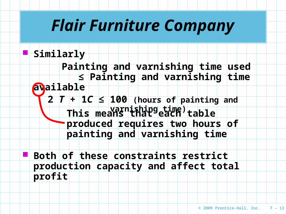
SimilarlyPainting and varnishing time used
≤ Painting and varnishing time available2 T + 1C ≤ 100 (hours of painting and varnishing time)
This means that each table produced requires two hours of painting and varnishing time
Both of these constraints restrict production capacity and affect total profit
© 2009 Prentice-Hall, Inc. 7 – 14
Flair Furniture Company
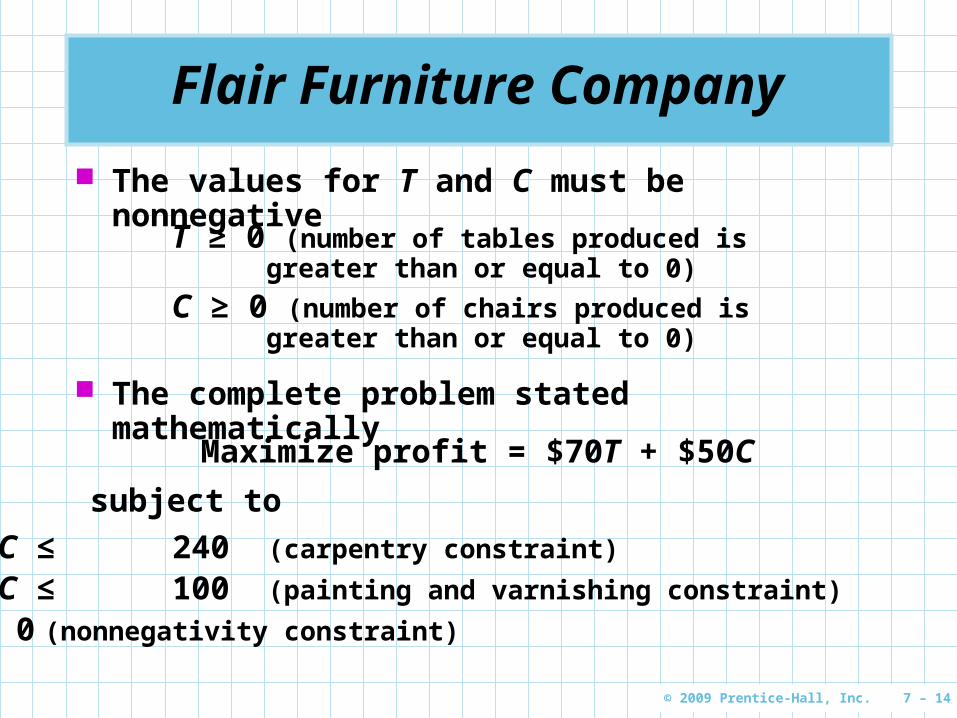
The values for T and C must be nonnegative
T ≥ 0 (number of tables produced is greater than or equal to 0)
C ≥ 0 (number of chairs produced is greater than or equal to 0)
The complete problem stated mathematically
Maximize profit = $70T + $50C
subject to
4T + 3C ≤240 (carpentry constraint)
2T + 1C ≤100 (painting and varnishing constraint)
T, C ≥ 0 (nonnegativity constraint)
© 2009 Prentice-Hall, Inc. 7 – 15
Graphical Solution to an LP Problem
The easiest way to solve a small LP problems is with the graphical solution approach
The graphical method only works when there are just two decision variables
When there are more than two variables, a more complex approach is needed as it is not possible to plot the solution on a two-dimensional graph
The graphical method provides valuable insight into how other approaches work

© 2009 Prentice-Hall, Inc. 7 – 16
Graphical Representation of a Constraint
100 –
–
80 –
–
60 –
–
40 –
–
20 –
–
–
C
| | | | | | | | | | | |
0 20 40 60 80 100 T
Nu
mb
er o
f C
hai
rs
Number of Tables
This Axis Represents the Constraint T ≥ 0
This Axis Represents the Constraint C ≥ 0
Figure 7.1

© 2009 Prentice-Hall, Inc. 7 – 17
Graphical Representation of a Constraint
The first step in solving the problem is to identify a set or region of feasible solutions
To do this we plot each constraint equation on a graph
We start by graphing the equality portion of the constraint equations
4T + 3C = 240 We solve for the axis intercepts and draw
the line
© 2009 Prentice-Hall, Inc. 7 – 18
Graphical Representation of a Constraint
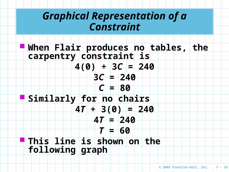
When Flair produces no tables, the carpentry constraint is
4(0) + 3C = 2403C = 240C = 80
Similarly for no chairs4T + 3(0) = 240
4T = 240T = 60
This line is shown on the following graph

© 2009 Prentice-Hall, Inc. 7 – 19
Graphical Representation of a Constraint
100 –
–
80 –
–
60 –
–
40 –
–
20 –
–
–
C
| | | | | | | | | | | |
0 20 40 60 80 100 T
Nu
mb
er o
f C
hai
rs
Number of Tables
(T = 0, C = 80)
Figure 7.2
(T = 60, C = 0)
Graph of carpentry constraint equation
© 2009 Prentice-Hall, Inc. 7 – 20
Graphical Representation of a Constraint
100 –
–
80 –
–
60 –
–
40 –
–
20 –
–
–
C
| | | | | | | | | | | |
0 20 40 60 80 100 T
Nu
mb
er o
f C
hai
rs
Number of TablesFigure 7.3
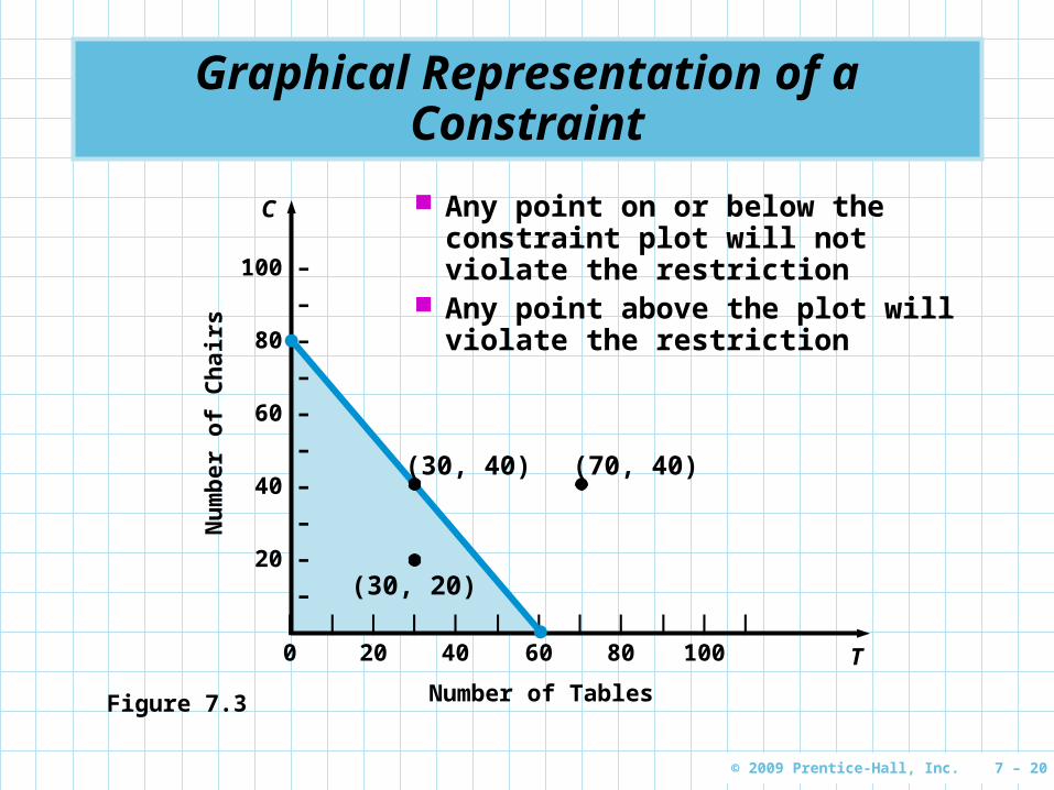
Any point on or below the constraint plot will not violate the restriction
Any point above the plot will violate the restriction
(30, 40)
(30, 20)
(70, 40)
© 2009 Prentice-Hall, Inc. 7 – 21
Graphical Representation of a Constraint
The point (30, 40) lies on the plot and exactly satisfies the constraint
4(30) + 3(40) = 240 The point (30, 20) lies below the plot and
satisfies the constraint
4(30) + 3(20) = 180 The point (30, 40) lies above the plot and
does not satisfy the constraint
4(70) + 3(40) = 400
© 2009 Prentice-Hall, Inc. 7 – 22
Graphical Representation of a Constraint
100 –
–
80 –
–
60 –
–
40 –
–
20 –
–
–
C
| | | | | | | | | | | |
0 20 40 60 80 100 T
Nu
mb
er o
f C
hai
rs
Number of Tables
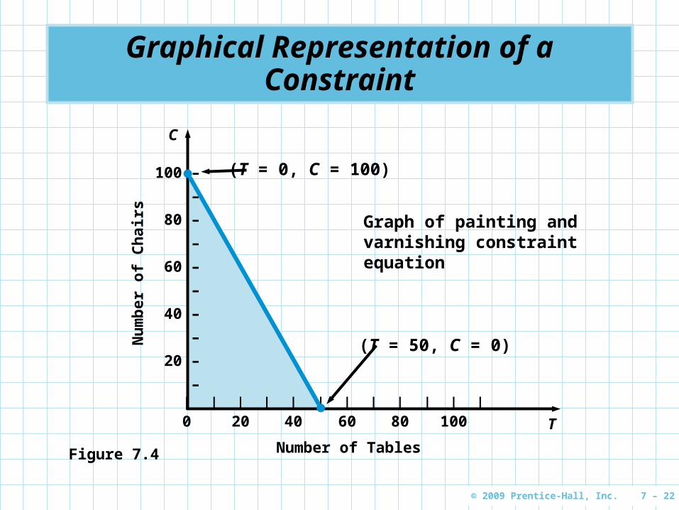
(T = 0, C = 100)
Figure 7.4
(T = 50, C = 0)
Graph of painting and varnishing constraint equation
© 2009 Prentice-Hall, Inc. 7 – 23
Graphical Representation of a Constraint
To produce tables and chairs, both departments must be used
We need to find a solution that satisfies both constraints simultaneouslysimultaneously
A new graph shows both constraint plots The feasible regionfeasible region (or area of feasible area of feasible
solutionssolutions) is where all constraints are satisfied Any point inside this region is a feasiblefeasible
solution Any point outside the region is an infeasibleinfeasible
solution

© 2009 Prentice-Hall, Inc. 7 – 24
Graphical Representation of a Constraint
100 –
–
80 –
–
60 –
–
40 –
–
20 –
–
–
C
| | | | | | | | | | | |
0 20 40 60 80 100 T
Nu
mb
er o
f C
hai
rs
Number of TablesFigure 7.5
Feasible solution region for Flair Furniture
Painting/Varnishing Constraint
Carpentry ConstraintFeasible Region
© 2009 Prentice-Hall, Inc. 7 – 25
Graphical Representation of a Constraint
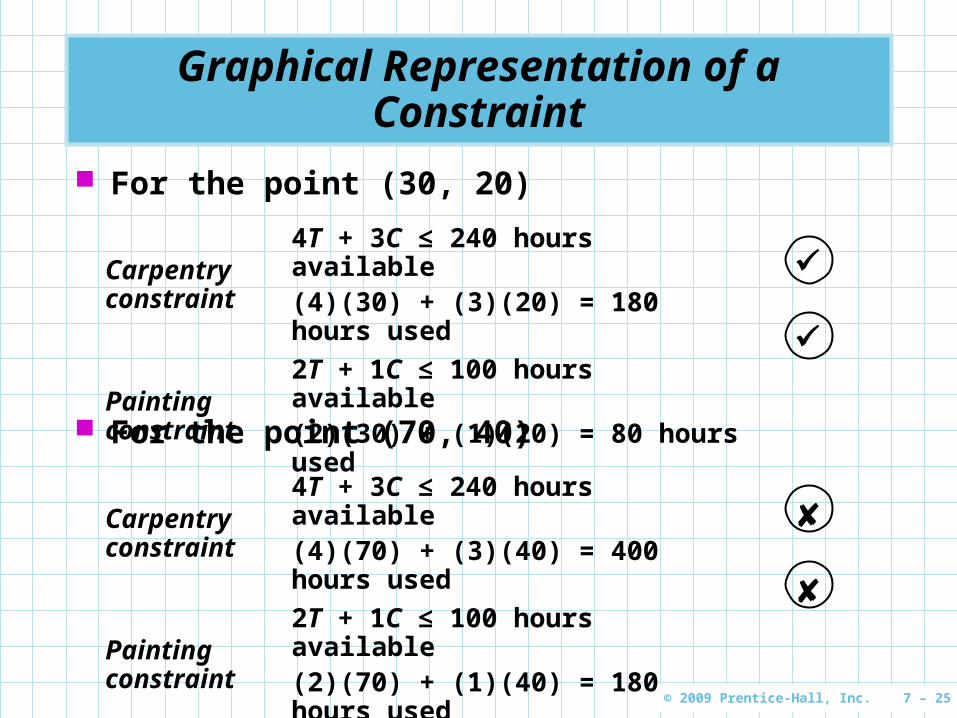
For the point (30, 20)
Carpentry constraint
4T + 3C ≤ 240 hours available(4)(30) + (3)(20) = 180 hours used
Painting constraint
2T + 1C ≤ 100 hours available(2)(30) + (1)(20) = 80 hours used
For the point (70, 40)
Carpentry constraint
4T + 3C ≤ 240 hours available(4)(70) + (3)(40) = 400 hours used
Painting constraint
2T + 1C ≤ 100 hours available(2)(70) + (1)(40) = 180 hours used
© 2009 Prentice-Hall, Inc. 7 – 26
Graphical Representation of a Constraint
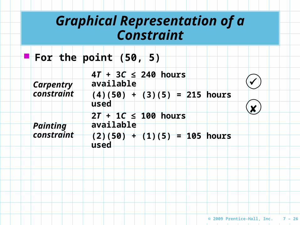
For the point (50, 5)
Carpentry constraint
4T + 3C ≤ 240 hours available(4)(50) + (3)(5) = 215 hours used
Painting constraint
2T + 1C ≤ 100 hours available(2)(50) + (1)(5) = 105 hours used
© 2009 Prentice-Hall, Inc. 7 – 27
Isoprofit Line Solution Method
Once the feasible region has been graphed, we need to find the optimal solution from the many possible solutions
The speediest way to do this is to use the isoprofit line method
Starting with a small but possible profit value, we graph the objective function
We move the objective function line in the direction of increasing profit while maintaining the slope
The last point it touches in the feasible region is the optimal solution
© 2009 Prentice-Hall, Inc. 7 – 28
Isoprofit Line Solution Method For Flair Furniture, choose a profit of $2,100 The objective function is then
$2,100 = 70T + 50C Solving for the axis intercepts, we can draw the
graph This is obviously not the best possible solution Further graphs can be created using larger profits The further we move from the origin while
maintaining the slope and staying within the boundaries of the feasible region, the larger the profit will be
The highest profit ($4,100) will be generated when the isoprofit line passes through the point (30, 40)
© 2009 Prentice-Hall, Inc. 7 – 29
100 –
–
80 –
–
60 –
–
40 –
–
20 –
–
–
C
| | | | | | | | | | | |
0 20 40 60 80 100 T
Nu
mb
er o
f C
hai
rs
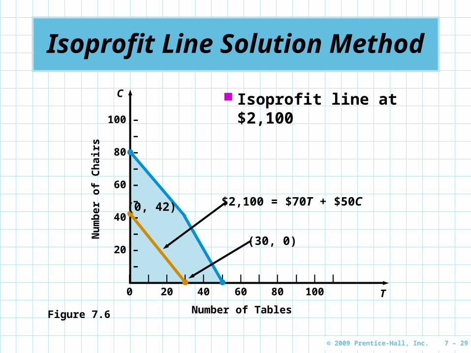
Number of TablesFigure 7.6
Isoprofit line at $2,100
$2,100 = $70T + $50C
(30, 0)
(0, 42)
Isoprofit Line Solution Method

© 2009 Prentice-Hall, Inc. 7 – 30
100 –
–
80 –
–
60 –
–
40 –
–
20 –
–
–
C
| | | | | | | | | | | |
0 20 40 60 80 100 T
Nu
mb
er o
f C
hai
rs
Number of TablesFigure 7.7
Four isoprofit lines
$2,100 = $70T + $50C
$2,800 = $70T + $50C
$3,500 = $70T + $50C
$4,100 = $70T + $50C
Isoprofit Line Solution Method
© 2009 Prentice-Hall, Inc. 7 – 31
100 –
–
80 –
–
60 –
–
40 –
–
20 –
–
–
C
| | | | | | | | | | | |
0 20 40 60 80 100 T
Nu
mb
er o
f C
hai
rs
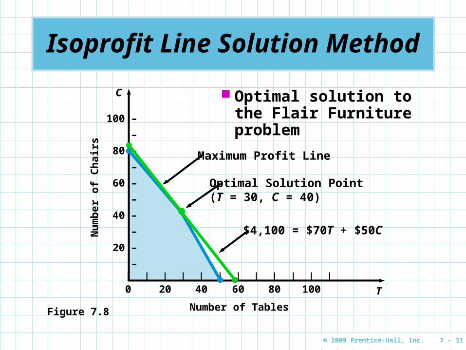
Number of TablesFigure 7.8
Optimal solution to the Flair Furniture problem
Optimal Solution Point(T = 30, C = 40)
Maximum Profit Line
$4,100 = $70T + $50C
Isoprofit Line Solution Method
© 2009 Prentice-Hall, Inc. 7 – 32
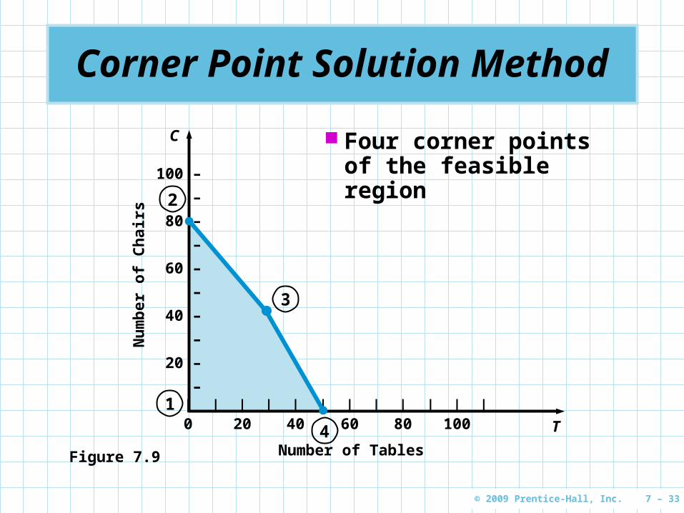
A second approach to solving LP problems employs the corner point methodcorner point method
It involves looking at the profit at every corner point of the feasible region
The mathematical theory behind LP is that the optimal solution must lie at one of the corner pointscorner points, or extreme pointextreme point, in the feasible region
For Flair Furniture, the feasible region is a four-sided polygon with four corner points labeled 1, 2, 3, and 4 on the graph
Corner Point Solution Method
© 2009 Prentice-Hall, Inc. 7 – 33
100 –
–
80 –
–
60 –
–
40 –
–
20 –
–
–
C
| | | | | | | | | | | |
0 20 40 60 80 100 T
Nu
mb
er o
f C
hai
rs
Number of TablesFigure 7.9
Four corner points of the feasible region
1
2
3
4
Corner Point Solution Method

© 2009 Prentice-Hall, Inc. 7 – 34
Corner Point Solution Method
3
1
2
4
Point : (T = 0, C = 0) Profit = $70(0) + $50(0) = $0
Point : (T = 0, C = 80) Profit = $70(0) + $50(80) = $4,000
Point : (T = 50, C = 0) Profit = $70(50) + $50(0) = $3,500
Point : (T = 30, C = 40) Profit = $70(30) + $50(40) = $4,100 Because Point returns the highest profit, this is the optimal solution
To find the coordinates for Point accurately we have to solve for the intersection of the two constraint lines
The details of this are on the following slide
3
3
© 2009 Prentice-Hall, Inc. 7 – 35
Corner Point Solution Method
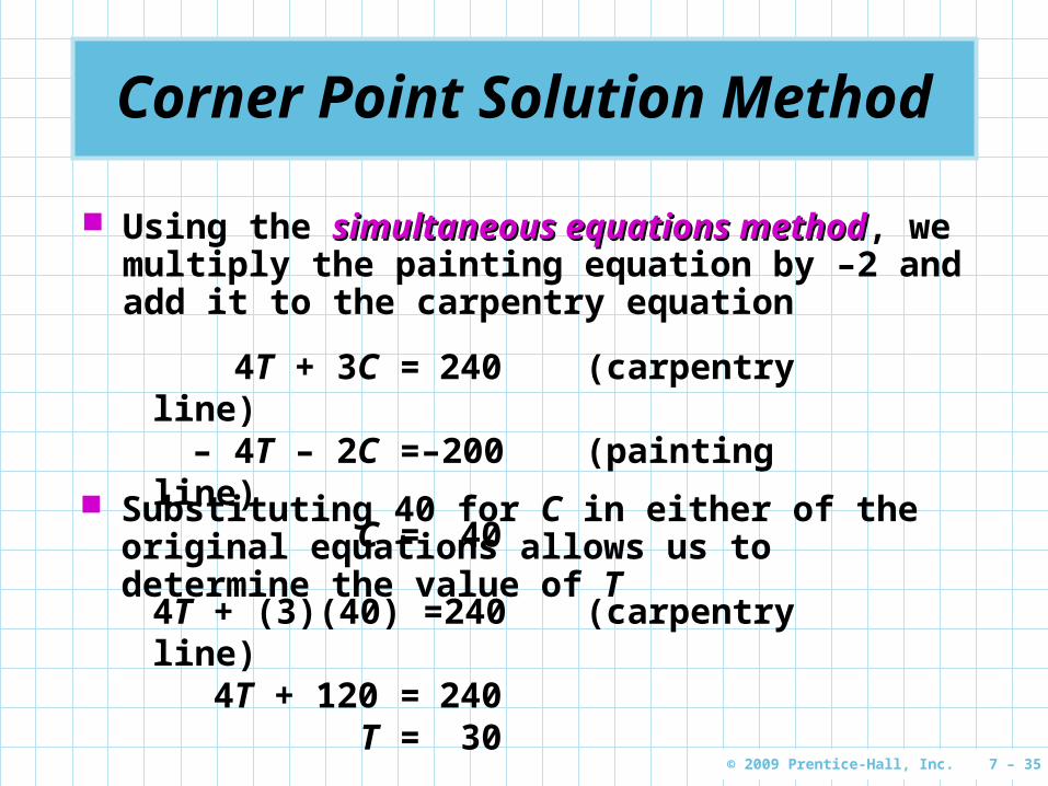
Using the simultaneous equations methodsimultaneous equations method, we multiply the painting equation by –2 and add it to the carpentry equation
4T + 3C = 240 (carpentry line)– 4T – 2C =–200 (painting line)
C = 40
Substituting 40 for C in either of the original equations allows us to determine the value of T
4T + (3)(40) = 240 (carpentry line)4T + 120 = 240
T = 30

© 2009 Prentice-Hall, Inc. 7 – 36
Summary of Graphical Solution Methods
ISOPROFIT METHOD
1. Graph all constraints and find the feasible region.
2. Select a specific profit (or cost) line and graph it to find the slope.
3. Move the objective function line in the direction of increasing profit (or decreasing cost) while maintaining the slope. The last point it touches in the feasible region is the optimal solution.
4. Find the values of the decision variables at this last point and compute the profit (or cost).
CORNER POINT METHOD
1. Graph all constraints and find the feasible region.
2. Find the corner points of the feasible reason.
3. Compute the profit (or cost) at each of the feasible corner points.
4. select the corner point with the best value of the objective function found in Step 3. This is the optimal solution.
Table 7.3

© 2009 Prentice-Hall, Inc. 7 – 37
Solving Flair Furniture’s LP Problem Using QM for Windows and Excel
Most organizations have access to software to solve big LP problems
While there are differences between software implementations, the approach each takes towards handling LP is basically the same
Once you are experienced in dealing with computerized LP algorithms, you can easily adjust to minor changes
© 2009 Prentice-Hall, Inc. 7 – 38
Using QM for Windows
First select the Linear Programming module Specify the number of constraints (non-negativity
is assumed) Specify the number of decision variables Specify whether the objective is to be maximized
or minimized For the Flair Furniture problem there are two
constraints, two decision variables, and the objective is to maximize profit
© 2009 Prentice-Hall, Inc. 7 – 39
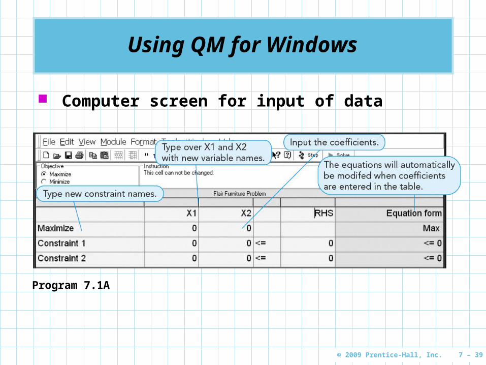
Using QM for Windows
Computer screen for input of data
Program 7.1A
© 2009 Prentice-Hall, Inc. 7 – 40
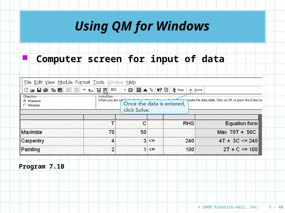
Using QM for Windows
Computer screen for input of data
Program 7.1B
© 2009 Prentice-Hall, Inc. 7 – 41
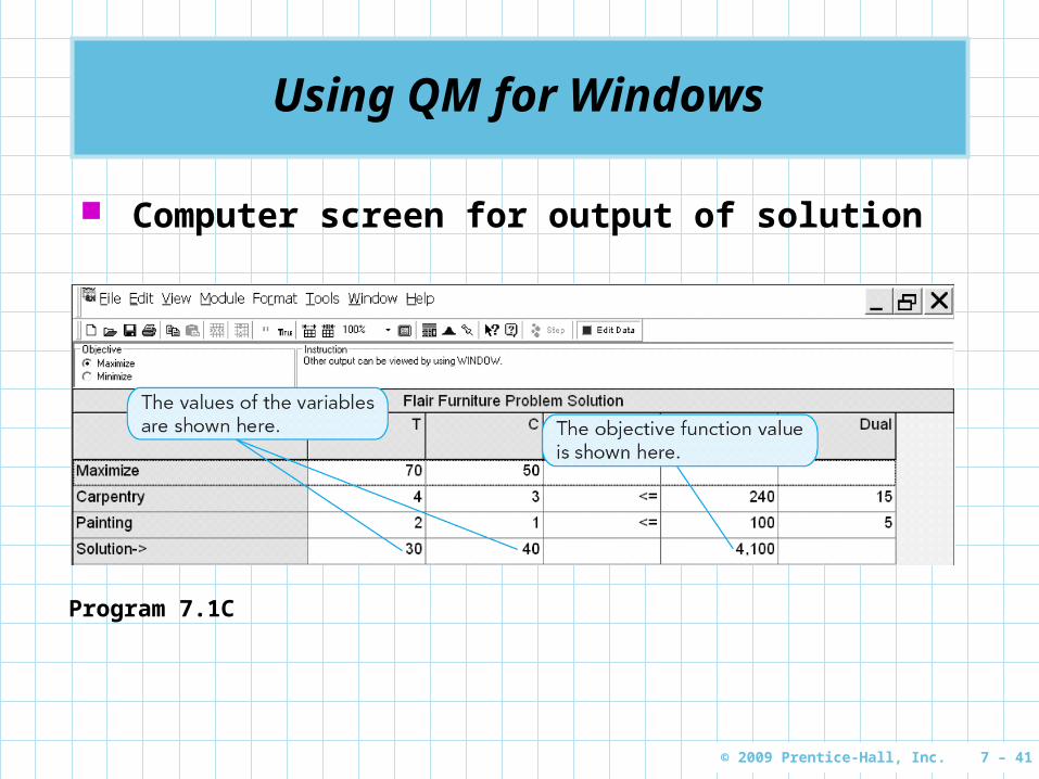
Using QM for Windows
Computer screen for output of solution
Program 7.1C

© 2009 Prentice-Hall, Inc. 7 – 42
Using QM for Windows
Graphical output of solution
Program 7.1D
© 2009 Prentice-Hall, Inc. 7 – 43
Solving Minimization Problems
Many LP problems involve minimizing an objective such as cost instead of maximizing a profit function
Minimization problems can be solved graphically by first setting up the feasible solution region and then using either the corner point method or an isocost line approach (which is analogous to the isoprofit approach in maximization problems) to find the values of the decision variables (e.g., X1 and X2) that yield the minimum cost
© 2009 Prentice-Hall, Inc. 7 – 44
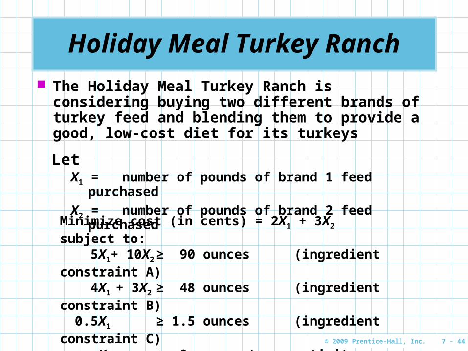
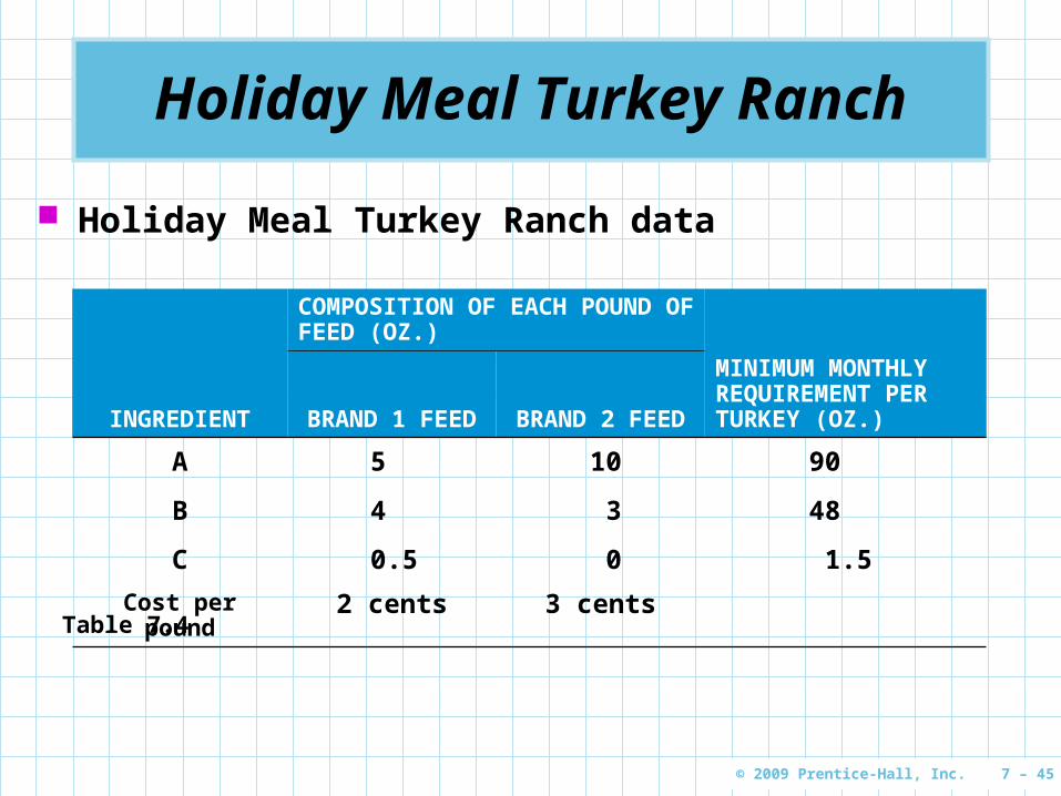
The Holiday Meal Turkey Ranch is considering buying two different brands of turkey feed and blending them to provide a good, low-cost diet for its turkeys
Minimize cost (in cents) = 2X1 + 3X2
subject to:5X1 + 10X2 ≥ 90 ounces (ingredient constraint A)4X1 + 3X2 ≥ 48 ounces (ingredient constraint B)
0.5X1 ≥ 1.5 ounces (ingredient constraint C) X1 ≥ 0 (nonnegativity constraint)
X2 ≥ 0 (nonnegativity constraint)
Holiday Meal Turkey Ranch
X1 = number of pounds of brand 1 feed purchased
X2 = number of pounds of brand 2 feed purchased
Let
© 2009 Prentice-Hall, Inc. 7 – 45
Holiday Meal Turkey Ranch
INGREDIENT
COMPOSITION OF EACH POUND OF FEED (OZ.)
MINIMUM MONTHLY REQUIREMENT PER TURKEY (OZ.)BRAND 1 FEED BRAND 2 FEED
A 5 10 90
B 4 3 48
C 0.5 0 1.5Cost per pound 2 cents 3 cents
Holiday Meal Turkey Ranch data
Table 7.4

© 2009 Prentice-Hall, Inc. 7 – 46
Using the corner point method
First we construct the feasible solution region
The optimal solution will lie at on of the corners as it would in a maximization problem
Holiday Meal Turkey Ranch
–
20 –
15 –
10 –
5 –
0 –
X2
| | | | | |
5 10 15 20 25 X1
Po
un
ds
of
Bra
nd
2
Pounds of Brand 1
Ingredient C Constraint
Ingredient B Constraint
Ingredient A Constraint
Feasible Region
a
b
c
Figure 7.10

© 2009 Prentice-Hall, Inc. 7 – 47
Holiday Meal Turkey Ranch
We solve for the values of the three corner points Point a is the intersection of ingredient constraints
C and B
4X1 + 3X2 = 48
X1 = 3 Substituting 3 in the first equation, we find X2 = 12 Solving for point b with basic algebra we find X1 =
8.4 and X2 = 4.8 Solving for point c we find X1 = 18 and X2 = 0

© 2009 Prentice-Hall, Inc. 7 – 48
Substituting these value back into the objective function we find
Cost = 2X1 + 3X2
Cost at point a = 2(3) + 3(12) = 42Cost at point b = 2(8.4) + 3(4.8) = 31.2Cost at point c = 2(18) + 3(0) = 36
Holiday Meal Turkey Ranch
The lowest cost solution is to purchase 8.4 pounds of brand 1 feed and 4.8 pounds of brand 2 feed for a total cost of 31.2 cents per turkey

© 2009 Prentice-Hall, Inc. 7 – 49
Using the isocost approach
Choosing an initial cost of 54 cents, it is clear improvement is possible
Holiday Meal Turkey Ranch
–
20 –
15 –
10 –
5 –
0 –
X2
| | | | | |
5 10 15 20 25 X1
Po
un
ds
of
Bra
nd
2
Pounds of Brand 1Figure 7.11
Feasible Region
54¢ = 2X1 + 3X
2 Isocost Line
Direction of Decreasing Cost
31.2¢ = 2X1 + 3X
2
(X1 = 8.4, X2 = 4.8)
© 2009 Prentice-Hall, Inc. 7 – 50
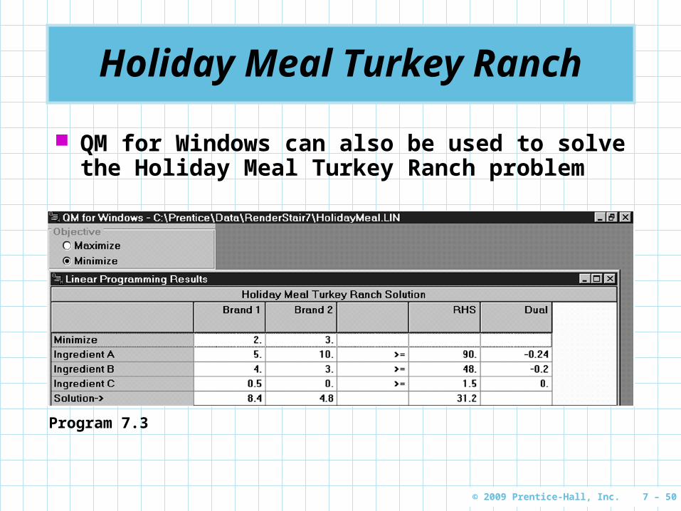
QM for Windows can also be used to solve the Holiday Meal Turkey Ranch problem
Holiday Meal Turkey Ranch
Program 7.3
© 2009 Prentice-Hall, Inc. 7 – 51
Assignment Problems Involve determining the most efficient way to
assign resources to tasks Objective may be to minimize travel times or
maximize assignment effectiveness Assignment problems are unique because they
have a coefficient of 0 or 1 associated with each variable in the LP constraints and the right-hand side of each constraint is always equal to 1
Employee Scheduling Applications
© 2009 Prentice-Hall, Inc. 7 – 52
Ivan and Ivan law firm maintains a large staff of young attorneys
Ivan wants to make lawyer-to-client assignments in the most effective manner
He identifies four lawyers who could possibly be assigned new cases
Each lawyer can handle one new client The lawyers have different skills and special
interests The following table summarizes the lawyers
estimated effectiveness on new cases
Employee Scheduling Applications
© 2009 Prentice-Hall, Inc. 7 – 53
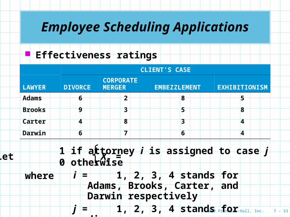
Effectiveness ratings
Employee Scheduling Applications
CLIENT’S CASE
LAWYER DIVORCECORPORATE MERGER EMBEZZLEMENT EXHIBITIONISM
Adams 6 2 8 5
Brooks 9 3 5 8
Carter 4 8 3 4
Darwin 6 7 6 4
Let Xij =1 if attorney i is assigned to case j0 otherwise
where i = 1, 2, 3, 4 stands for Adams, Brooks, Carter, and Darwin respectively
j = 1, 2, 3, 4 stands for divorce, merger, embezzlement, and exhibitionism

© 2009 Prentice-Hall, Inc. 7 – 54
The LP formulation is
Employee Scheduling Applications
Maximize effectiveness =6X11 + 2X12 + 8X13 + 5X14 + 9X21 + 3X22
+ 5X23 + 8X24 + 4X31 + 8X32 + 3X33 + 4X34
+ 6X41 + 7X42 + 6X43 + 4X44
subject to X11 + X21 + X31 + X41 = 1 (divorce case)
X12 + X22 + X32 + X42 = 1 (merger)
X13 + X23 + X33 + X43 = 1 (embezzlement)
X14 + X24 + X34 + X44 = 1 (exhibitionism)
X11 + X12 + X13 + X14 = 1 (Adams)
X21 + X22 + X23 + X24 = 1 (Brook)
X31 + X32 + X33 + X34 = 1 (Carter)
X41 + X42 + X43 + X44 = 1 (Darwin)

© 2009 Prentice-Hall, Inc. 7 – 55
Solving Ivan and Ivan’s assignment scheduling LP problem using QM for Windows
Employee Scheduling Applications
Program 8.4

© 2009 Prentice-Hall, Inc. 7 – 56
Four Special Cases in LP
Four special cases and difficulties arise at times when using the graphical approach to solving LP problems Infeasibility Unboundedness Redundancy Alternate Optimal Solutions

© 2009 Prentice-Hall, Inc. 7 – 57
Four Special Cases in LP
No feasible solution Exists when there is no solution to the
problem that satisfies all the constraint equations
No feasible solution region exists This is a common occurrence in the real world Generally one or more constraints are relaxed
until a solution is found
© 2009 Prentice-Hall, Inc. 7 – 58
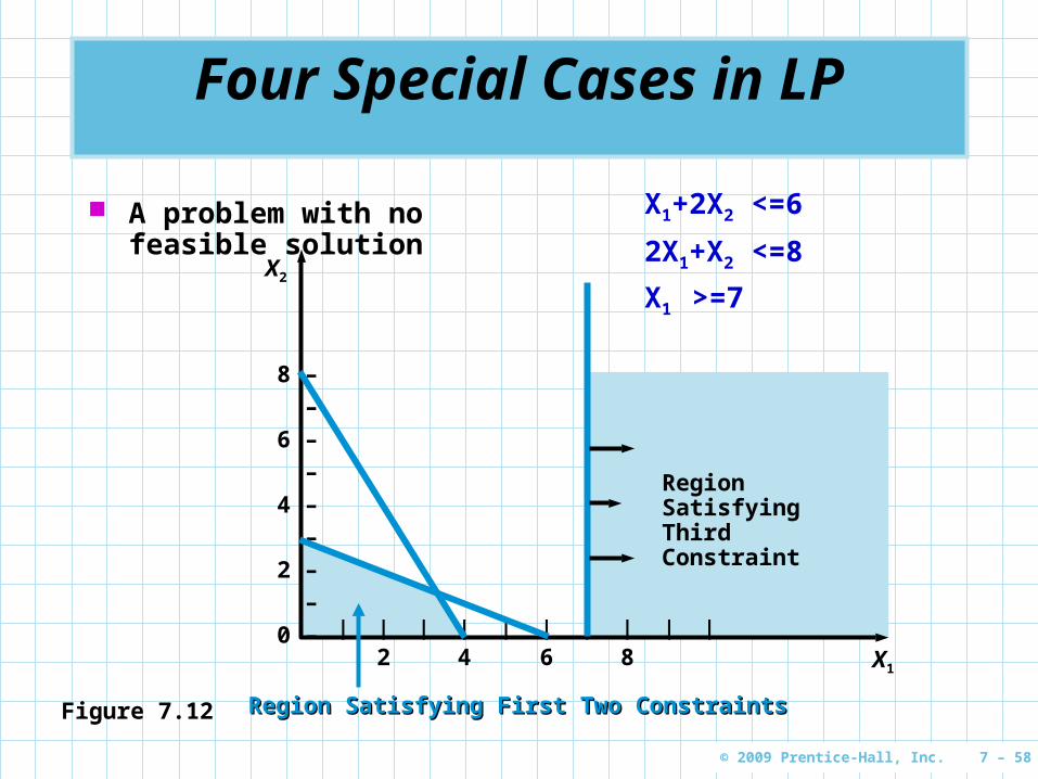
Four Special Cases in LP
A problem with no feasible solution
8 –
–
6 –
–
4 –
–
2 –
–
0 –
X2
| | | | | | | | | |
2 4 6 8 X1
Region Satisfying First Two ConstraintsRegion Satisfying First Two ConstraintsFigure 7.12
Region Satisfying Third Constraint
X1+2X2 <=6
2X1+X2 <=8
X1 >=7
© 2009 Prentice-Hall, Inc. 7 – 59
Four Special Cases in LP
Unboundedness Sometimes a linear program will not have a
finite solution In a maximization problem, one or more
solution variables, and the profit, can be made infinitely large without violating any constraints
In a graphical solution, the feasible region will be open ended
This usually means the problem has been formulated improperly

© 2009 Prentice-Hall, Inc. 7 – 60
Four Special Cases in LP
A solution region unbounded to the right
15 –
10 –
5 –
0 –
X2
| | | | |
5 10 15 X1
Figure 7.13
Feasible Region
X1 ≥ 5
X2 ≤ 10
X1 + 2X2 ≥ 15
© 2009 Prentice-Hall, Inc. 7 – 61
Four Special Cases in LP
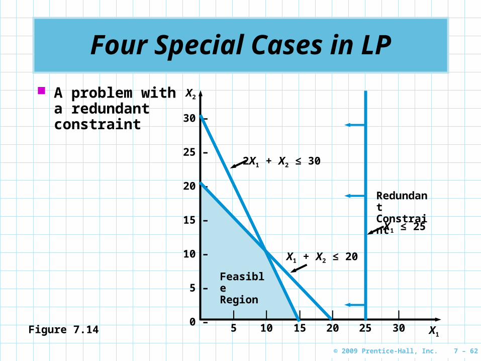
Redundancy A redundant constraint is one that does not
affect the feasible solution region One or more constraints may be more binding This is a very common occurrence in the real
world It causes no particular problems, but
eliminating redundant constraints simplifies the model
© 2009 Prentice-Hall, Inc. 7 – 62
Four Special Cases in LP
A problem with a redundant constraint
30 –
25 –
20 –
15 –
10 –
5 –
0 –
X2
| | | | | |
5 10 15 20 25 30 X1Figure 7.14
Redundant Constraint
Feasible Region
X1 ≤ 25
2X1 + X2 ≤ 30
X1 + X2 ≤ 20
© 2009 Prentice-Hall, Inc. 7 – 63
Four Special Cases in LP
Alternate Optimal Solutions Occasionally two or more optimal solutions
may exist Graphically this occurs when the objective
function’s isoprofit or isocost line runs perfectly parallel to one of the constraints
This actually allows management great flexibility in deciding which combination to select as the profit is the same at each alternate solution
© 2009 Prentice-Hall, Inc. 7 – 64
Four Special Cases in LP
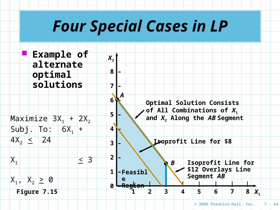
Example of alternate optimal solutions
8 –
7 –
6 –
5 –
4 –
3 –
2 –
1 –
0 –
X2
| | | | | | | |
1 2 3 4 5 6 7 8 X1Figure 7.15
Feasible Region
Isoprofit Line for $8
Optimal Solution Consists of All Combinations of X1 and X2 Along the AB Segment
Isoprofit Line for $12 Overlays Line Segment AB
B
A
Maximize 3X1 + 2X2
Subj. To: 6X1 + 4X2 < 24 X1 < 3 X1, X2 > 0

© 2009 Prentice-Hall, Inc. 7 – 65
Sensitivity Analysis
Optimal solutions to LP problems thus far have been found under what are called deterministic deterministic assumptionsassumptions
This means that we assume complete certainty in the data and relationships of a problem
But in the real world, conditions are dynamic and changing
We can analyze how sensitivesensitive a deterministic solution is to changes in the assumptions of the model
This is called sensitivity analysissensitivity analysis, postoptimality postoptimality analysisanalysis, parametric programmingparametric programming, or optimality optimality analysisanalysis
© 2009 Prentice-Hall, Inc. 7 – 66
Sensitivity Analysis
Sensitivity analysis often involves a series of what-if? questions concerning constraints, variable coefficients, and the objective function
What if the profit for product 1 increases by 10%? What if less advertising money is available?
One way to do this is the trial-and-error method where values are changed and the entire model is resolved
The preferred way is to use an analytic postoptimality analysis
After a problem has been solved, we determine a range of changes in problem parameters that will not affect the optimal solution or change the variables in the solution without re-solving the entire problem

© 2009 Prentice-Hall, Inc. 7 – 67
Sensitivity Analysis
Sensitivity analysis can be used to deal not only with errors in estimating input parameters to the LP model but also with management’s experiments with possible future changes in the firm that may affect profits.
© 2009 Prentice-Hall, Inc. 7 – 68
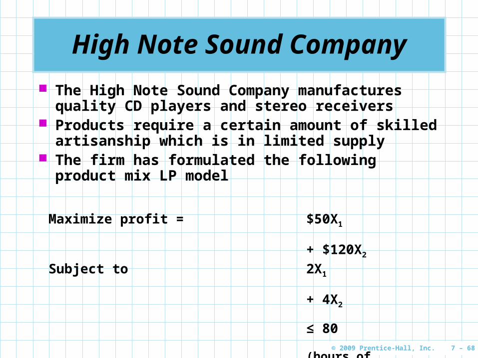
The High Note Sound Company manufactures quality CD players and stereo receivers
Products require a certain amount of skilled artisanship which is in limited supply
The firm has formulated the following product mix LP model
High Note Sound Company
Maximize profit = $50X1
+ $120X2
Subject to 2X1
+ 4X2
≤ 80
(hours of electrician’s time available)
3X1
+ 1X2
≤ 60
(hours of audio technician’s time available)
X1, X2
≥ 0
© 2009 Prentice-Hall, Inc. 7 – 69
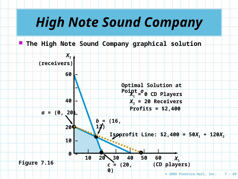
The High Note Sound Company graphical solution
High Note Sound Company
b = (16, 12)
Optimal Solution at Point a
X1 = 0 CD PlayersX2 = 20 ReceiversProfits = $2,400
a = (0, 20)
Isoprofit Line: $2,400 = 50X1 + 120X2
60 –
–
40 –
–
20 –
10 –
0 –
X2
| | | | | |
10 20 30 40 50 60 X1
(receivers)
(CD players)c = (20, 0)Figure 7.16
© 2009 Prentice-Hall, Inc. 7 – 70
Changes in the Objective Function Coefficient
In real-life problems, contribution rates in the objective functions fluctuate periodically
Graphically, this means that although the feasible solution region remains exactly the same, the slope of the isoprofit or isocost line will change
We can often make modest increases or decreases in the objective function coefficient of any variable without changing the current optimal corner point
We need to know how much an objective function coefficient can change before the optimal solution would be at a different corner point

© 2009 Prentice-Hall, Inc. 7 – 71
Changes in the Objective Function Coefficient
Changes in the receiver contribution coefficients
ba
Profit Line for 50X1 + 80X2
(Passes through Point b)
40 –
30 –
20 –
10 –
0 –
X2
| | | | | |
10 20 30 40 50 60 X1
c
Figure 7.17
Profit Line for 50X1 + 120X2
(Passes through Point a)
Profit Line for 50X1 + 150X2
(Passes through Point a)
© 2009 Prentice-Hall, Inc. 7 – 72
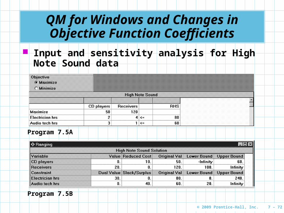
QM for Windows and Changes in Objective Function Coefficients
Input and sensitivity analysis for High Note Sound data
Program 7.5B
Program 7.5A

© 2009 Prentice-Hall, Inc. 7 – 73
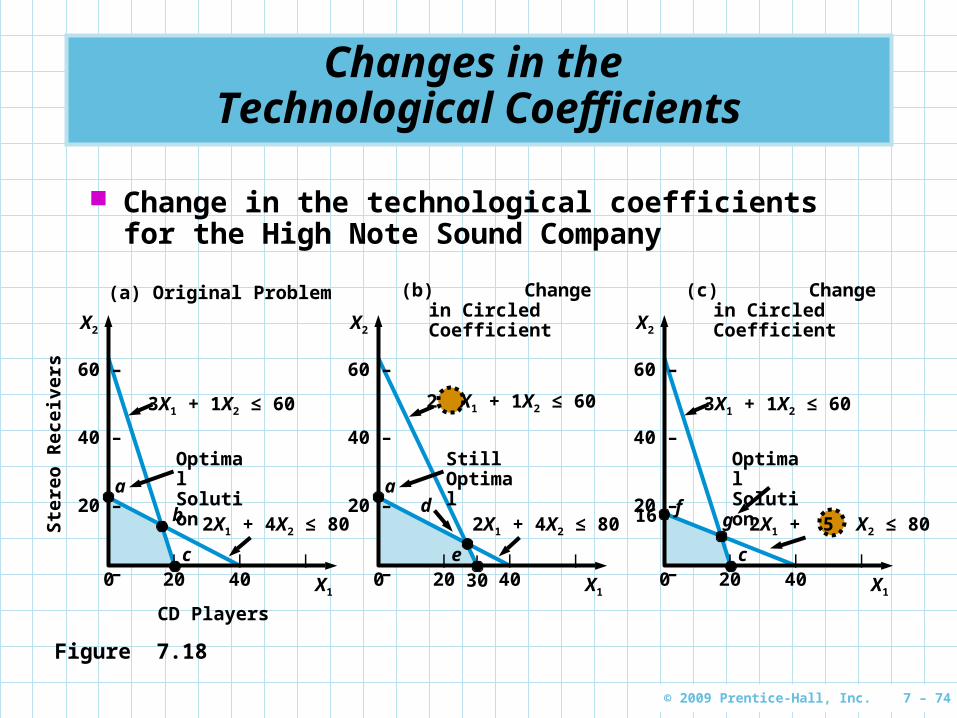
Changes in the Technological Coefficients
Changes in the technological coefficientstechnological coefficients often reflect changes in the state of technology
If the amount of resources needed to produce a product changes, coefficients in the constraint equations will change
This does not change the objective function, but it can produce a significant change in the shape of the feasible region
This may cause a change in the optimal solution
© 2009 Prentice-Hall, Inc. 7 – 74
Changes in the Technological Coefficients
Change in the technological coefficients for the High Note Sound Company
(a) Original Problem
3X1 + 1X2 ≤ 60
2X1 + 4X2 ≤ 80
Optimal Solution
X2
60 –
40 –
20 –
–| | |
0 20 40 X1
Ste
reo
Rec
eiv
ers
CD Players
(b) Change in Circled Coefficient
2 X1 + 1X2 ≤ 60
2X1 + 4X2 ≤ 80
Still Optimal
3X1 + 1X2 ≤ 60
2X1 + 5 X2 ≤ 80
Optimal Solutiona
d
e
60 –
40 –
20 –
–| | |
0 20 40
X2
X1
16
60 –
40 –
20 –
–| | |
0 20 40
X2
X1
|
30
(c) Change in Circled Coefficient
a
b
c
fg
c
Figure 7.18
© 2009 Prentice-Hall, Inc. 7 – 75
Changes in Resources or Right-Hand-Side Values
The right-hand-side values of the constraints often represent resources available to the firm
If additional resources were available, a higher total profit could be realized
Sensitivity analysis about resources will help answer questions such as: How much should the company be willing to pay
for additional hours? Is it profitable to have some electricians work
overtime? Should we be willing to pay for more audio
technician time?
© 2009 Prentice-Hall, Inc. 7 – 76
Changes in Resources or Right-Hand-Side Values
If the right-hand side of a constraint is changed, the feasible region will change (unless the constraint is redundant) and often the optimal solution will change
The amount of change (increase or decrease) in the objective function value that results from a unit change in one of the resources available is called the dual dual priceprice or dual valuedual value
© 2009 Prentice-Hall, Inc. 7 – 77
Changes in Resources or Right-Hand-Side Values
However, the amount of possible increase in the right-hand side of a resource is limited
If the number of hours increases beyond the upper bound (or decreases below the lower bound), then the objective function would no longer increase (decrease) by the dual price. There may be excess (slack) hours of a resource
or the objective function may change by an amount different from the dual price.
Thus, the dual price is relevant only within limits. If the dual value of a constraint is zero
The slack is positive, indicating unused resource Additional amount of resource will simply increase
the amount of slack. The upper limit of infinity indicates that adding
more hours would simply increase the amount of slack.
© 2009 Prentice-Hall, Inc. 7 – 78
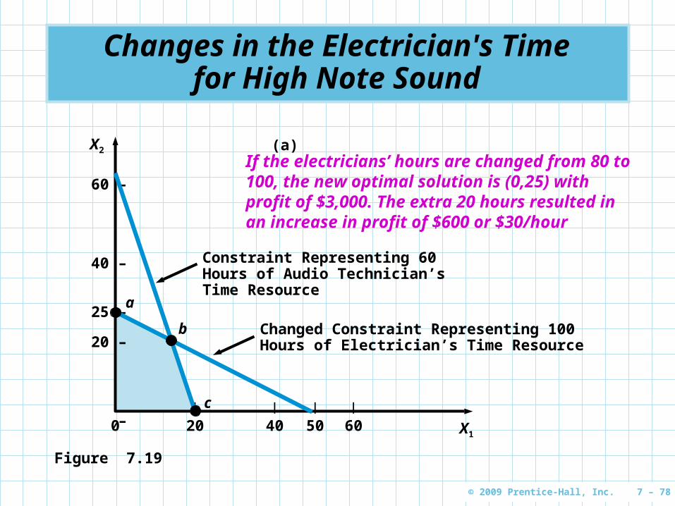
Changes in the Electrician's Time for High Note Sound
60 –
40 –
20 –
–
25 –
| | |
0 20 40 60|
50 X1
X2 (a)
a
b
c
Constraint Representing 60 Hours of Audio Technician’s Time Resource
Changed Constraint Representing 100 Hours of Electrician’s Time Resource
Figure 7.19
If the electricians’ hours are changed from 80 to 100, the new optimal solution is (0,25) with profit of $3,000. The extra 20 hours resulted in an increase in profit of $600 or $30/hour
© 2009 Prentice-Hall, Inc. 7 – 79
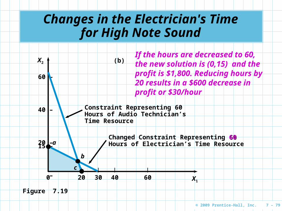
Changes in the Electrician's Time for High Note Sound
60 –
40 –
20 –
–
15 –
| | |
0 20 40 60|
30 X1
X2 (b)
a
b
c
Constraint Representing 60 Hours of Audio Technician’s Time Resource
Changed Constraint Representing 6060 Hours of Electrician’s Time Resource
Figure 7.19
If the hours are decreased to 60, the new solution is (0,15) and the profit is $1,800. Reducing hours by 20 results in a $600 decrease in profit or $30/hour
© 2009 Prentice-Hall, Inc. 7 – 80
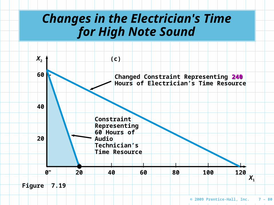
Changes in the Electrician's Time for High Note Sound
60 –
40 –
20 –
–| | | | | |
0 20 40 60 80 100 120X1
X2 (c)
Constraint Representing 60 Hours of Audio Technician’s Time Resource
Changed Constraint Representing 240240 Hours of Electrician’s Time Resource
Figure 7.19
© 2009 Prentice-Hall, Inc. 7 – 81
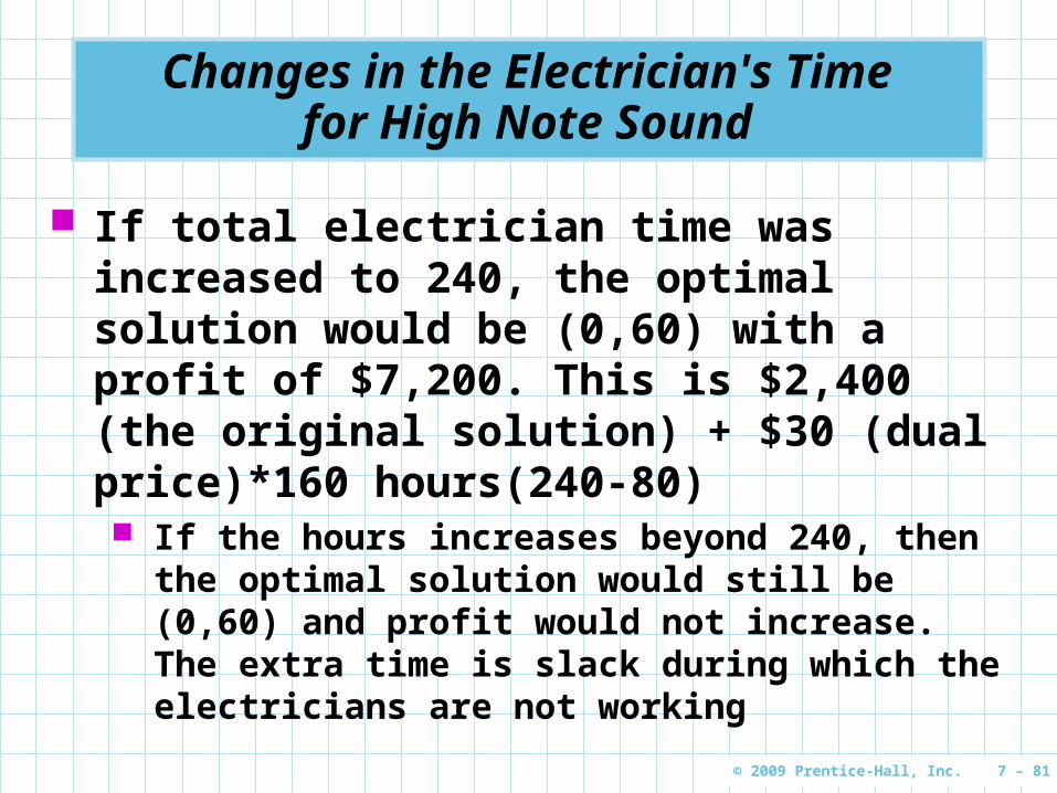
Changes in the Electrician's Time for High Note Sound
If total electrician time was increased to 240, the optimal solution would be (0,60) with a profit of $7,200. This is $2,400 (the original solution) + $30 (dual price)*160 hours(240-80) If the hours increases beyond 240, then the
optimal solution would still be (0,60) and profit would not increase. The extra time is slack during which the electricians are not working

© 2009 Prentice-Hall, Inc. 7 – 82
QM for Windows and Changes in Right-Hand-Side Values
Input and sensitivity analysis for High Note Sound data
Program 7.5B
Program 7.5A

© 2009 Prentice-Hall, Inc. 7 – 83
Flair Furniture – Sensitivity Analysis
Dual/ValueDual/Value RHS changeRHS change Solution changeSolution change
Carpentry/1.5 240241 30/40: 410
29.5/41: 411.5
Painting/.5 100101 30/40: 410
31.5/38: 410.5
Profit per itemProfit per item SolutionSolution RangeRange
Table 7 6.67 10
Chair 5 3.5 5.25
© 2009 Prentice-Hall, Inc. 7 – 84
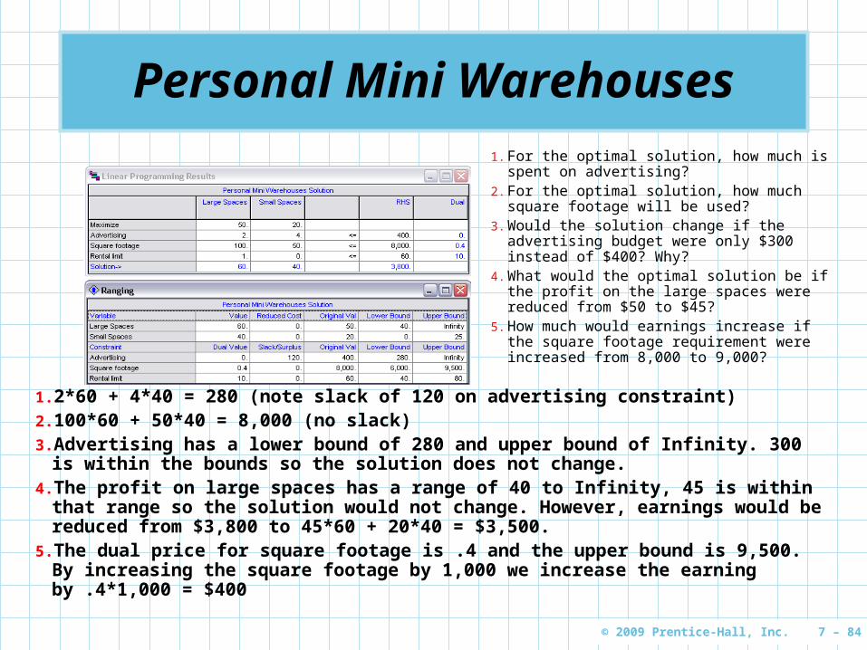
Personal Mini Warehouses1. For the optimal solution, how much is spent on
advertising?2. For the optimal solution, how much square footage
will be used?3. Would the solution change if the advertising budget
were only $300 instead of $400? Why?4. What would the optimal solution be if the profit on
the large spaces were reduced from $50 to $45?5. How much would earnings increase if the square
footage requirement were increased from 8,000 to 9,000?
1. 2*60 + 4*40 = 280 (note slack of 120 on advertising constraint)2. 100*60 + 50*40 = 8,000 (no slack)3. Advertising has a lower bound of 280 and upper bound of Infinity. 300 is within the
bounds so the solution does not change.4. The profit on large spaces has a range of 40 to Infinity, 45 is within that range so the
solution would not change. However, earnings would be reduced from $3,800 to 45*60 + 20*40 = $3,500.
5. The dual price for square footage is .4 and the upper bound is 9,500. By increasing the square footage by 1,000 we increase the earning by .4*1,000 = $400