ZETA POTENTIAL AND COLLOID CHEMISTRY

Eric Olson

ABSTRACT

The US Food and Drug Administration often requests the measurement of zeta potential; however, there is

virtually no guidance offered in any of the regulatory pharmacopoeias. Guidelines are available in other

standards, and there exists a wealth of information in texts and publications. Many of these are taken from

non-pharmaceutical industries where zeta potential is routinely used as part of quality control criteria.

This discussion outlines current guidance to aid quality units with potential issues and questions; reviews

the complex topics of colloid chemistry and zeta potential; and provides insight to chemists who may

require zeta potential determination, but who may not be well versed in these topics.

Basic colloid principles are discussed including definitions, types of colloidal systems, and common

properties. Types of colloidal particles, micelles, and surrounding layers are detailed. Colloidal stability is

discussed. Electrokinetic effects and underlying theories by which electrophoretic mobility is used to

calculate zeta potential are detailed. Sample preparation, the importance of sample history, determination of

zeta potential, and isoelectric point measurement are discussed.

INTRODUCTION

The determination of zeta potential is often required when a pharmaceutical formulation involves micelles

or when the shelf life of a product that contains fine particles is in question. For the sake of this discussion,

fine particles are defined as those with a mean diameter of 10µm or less. FDA often requests

pharmaceutical manufacturers and formulators to provide zeta potential data.

Zeta potential is a frequently misunderstood phenomenon. Zeta potential is rarely taught in most collegiate

curricula. There is no guidance offered in the United States Pharmacopoeia, National Formulary

(USP/NF), the British Pharmacopoeia (BP), the European Pharmacopoeia (EP), the Japanese

Pharmacopoeia (JP), or in current International Conference on Harmonization (ICH) guidelines on the

definition, determination, or reporting of zeta potential. There was an American Society for Testing and

Materials (ASTM) standard, D4187-82 in effect, but that standard was retired and not replaced (1). More

recently, the International Organization for Standardization (ISO) published two draft standards related to

zeta potential and prepared a third, which has not yet been released (2-4). In addition, the International

Union of Pure and Applied Chemists (IUPAC) published some guidelines (5).

Zeta potential, per the IUPAC definition, is “The potential at the plane where slip with respect to bulk

solution is postulated to occur is identified as the electrokinetic or zeta potential, ζ” (5). In simplified terms,

it is a determination of the charge between two particles that keeps them separated from one another. It is

important to note zeta potential is the potential at the slip plane, not the charge on the surface of the particle

as is often assumed. Furthermore, zeta potential is a colloidal determination that is typically performed on a

liquid-liquid system or a solid-liquid system. It is not to be confused with the static charge or electrostatic

potential developed by moving or processing a dry powder.

It is also important to distinguish between a solution and dispersion. A solution is defined as a system in

which a solute is dissolved in a solvent. A colloidal system sometimes referred to as a dispersion,

suspension, or sol, consists of a dispersed phase, which is distributed uniformly in a continuous phase.

There are two primary forces at work on colloidal systems: long range, weak, Van der Waals attractions and

short range, stronger, electrostatic repulsions. It is the sum of the weak attractive and strong repulsive

forces that are responsible for colloidal stability. Thus, the greater the magnitudes of the zeta potential, the

more stable the colloidal dispersion. Because zeta potential is related to colloidal stability, it is often

correlated to properties such as shelf life, material stability, and end-user mixing requirements. Though a

zeta potential of high magnitude is often considered ideal, that is not always the case. In some applications

(e.g., wastewater treatment) a low zeta potential is often desired. A low zeta potential can be established

that will induce flocculation of the particles and aid in the water clarification process.

METHOD VALIDATION

Good manufacturing practice (GMP) method validations typically include specificity, linearity, range,

accuracy, precision, and robustness. Specificity and linearity are not applicable to the determination of zeta

potential. Range can be a difficult factor to assess because no single sample type can be used that will span

the entire range of the instrument technique. There is no National Institute of Standards and Technology

(NIST) traceable certified reference material for zeta potential to date, though several of the zeta potential

instrument manufacturers offer a reference standard that is used for the purposes of determining accuracy

and system suitability.

The electrokinetic effect known as electrophoretic mobility is normally measured and from that, the zeta

potential is calculated. Per the draft ISO standard 13099-2, the accuracy is considered acceptable if the

mean electrophoretic mobility value is within 10% of the published value (3). The repeatability of three

measurements is considered acceptable if the coefficient of variation for the mean electrophoretic mobility

values is less than 10%. The intermediate precision is considered acceptable if the coefficient of variation

for the mean electrophoretic mobility value is less than 15%.

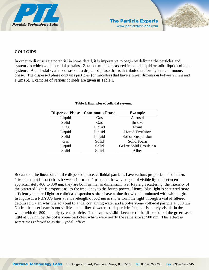
COLLOIDS

In order to discuss zeta potential in some detail, it is imperative to begin by defining the particles and

systems to which zeta potential pertains. Zeta potential is measured in liquid-liquid or solid-liquid colloidal

systems. A colloidal system consists of a dispersed phase that is distributed uniformly in a continuous

phase. The dispersed phase contains particles (or micelles) that have a linear dimension between 1 nm and

1 m (6). Examples of various colloids are given in Table I.

Table I: Examples of colloidal systems.

Dispersed Phase Continuous Phase Example

Liquid Gas Aerosol

Solid Gas Smoke

Gas Liquid Foam

Liquid Liquid Liquid Emulsion

Solid Liquid Sol or Suspension

Gas Solid Solid Foam

Liquid Solid Gel or Solid Emulsion

Solid Solid Alloy

Because of the linear size of the dispersed phase, colloidal particles have various properties in common.

Given a colloidal particle is between 1 nm and 1 m, and the wavelength of visible light is between

approximately 400 to 800 nm, they are both similar in dimension. Per Rayleigh scattering, the intensity of

the scattered light is proportional to the frequency to the fourth power. Hence, blue light is scattered more

efficiently than red light so colloidal dispersions often have a blue tint when illuminated with white light.

In Figure 1, a Nd:YAG laser at a wavelength of 532 nm is shone from the right through a vial of filtered

deionized water, which is adjacent to a vial containing water and a polystyrene colloidal particle at 500 nm.

Notice the laser beam is not visible in the filtered water that is particle-free, but is clearly visible in the

water with the 500 nm polystyrene particle. The beam is visible because of the dispersion of the green laser

light at 532 nm by the polystyrene particles, which were nearly the same size at 500 nm. This effect is

sometimes referred to as the Tyndall effect.

Figure 1: Illustration of the Tyndall effect.

Due to the very small particle size of a colloidal particle, Brownian motion is sufficient to keep them

suspended (7). At some point, the suspension of a particle by Brownian motion will be overcome by

gravity and become subject to Stokes’ law (8). Stokes’ law is given as Equation 1, where v is the settling

velocity, d is the particle diameter, g is gravitational acceleration, is the difference in density between

the particle and the continuous phase, and is the continuous phase viscosity.

18

2

gdv [Equation 1]

Another property that colloids have in common is a very high surface-to-volume ratio. As an example,

consider two spheres, one with a radius = 0.250 m and one with a radius = 100 m. The resulting surface

area and volumes are given in Table II. The exceptionally high surface area-to-volume ratio of the colloidal

sphere illustrates the importance of surface chemistry in the colloidal domain. As one might expect, the

behavior and stability of colloidal dispersions is dependent on the surface chemistry of the colloidal

particles.

Table II: Surface area-to-volume ratios.

Radius Surface Area Volume Surface Area/Volume

0.250 m 7.85X10-1

m2 6.54X10

-2 m

3 12.0 m

2/m

3

100 m 1.26X105 m

2 4.19X10

6 m

3 0.03 m

2/m

3

TYPES OF COLLOIDAL PARTICLES

Definitions and terminology associated with colloids are used in an inconsistent manner. Many texts define

aggregation and agglomeration one way and others define them the opposite way. There were also a large

number of texts that chose not to use the term “aggregate,” but term all particles larger than a primary

particle an “agglomerate.” Terminology used in this discussion will follow the definitions in the ISO

standard on sample preparation (9). It is important to know the type of colloidal particle for which zeta

potential is to be measured to ensure the resulting zeta potential data are applicable to the system of interest.

Primary Particle

A primary particle is one that may be defined as the smallest unit or structure from which other structures

are built. A primary particle may be a single crystal, a micelle, or even a small structure such as a

polymeric sphere.

Coalescence

Certain primary particles may come together and coalesce. This generates a larger particle with a change in

surface area compared to the sum of surface areas of the individual primary particles. A common example

of coalescence, though not on the colloidal scale, is what happens with puddles of mercury. Two small

puddles coalesce into a larger one with roughly the same shape, but with a decrease in total surface area.

Ripening

If the colloidal particle has some solubility in the continuous phase, a different phenomenon may occur.

Small particles generally exhibit more surface strain, which leads to higher surface energy and an increase

in solubility. Thus, the preferential solubility of the small particles will be greater than that compared to the

larger particles. Over time, the population of small particles will dissolve into solution. Sometimes the

dissolved material from the small particles will then deposit on the larger particles, making them even

larger. This process is known as Ostwald ripening (10-12).

Aggregation

Primary particles may also undergo a process by which they come in close contact, stick to each other, and

often form strong chemical bonds over a small area or point of contact. This process is called aggregation

or in some references, coagulation. Aggregates of very small or few primary particles may still be in the

colloidal size domain. Because of the bonds between the primary particles, they are most often quite

difficult to separate by normal means. Note that the process of aggregation may or may not result in an

appreciable difference in surface area. Whether it does is often dependent on the particle shape, the degree

of particle-particle contact, and the extent of three-dimensional packing.

Agglomeration

The final type of colloidal particles to be mentioned is that of agglomeration, or in some references,

flocculation. Primary particles or aggregates come in close contact and stick to each other by means of

weak, long-range bonds such as hydrogen bonding by this mechanism. Agglomerates are often outside the

colloidal size domain, but not always. Because the bonds are weak and typically long range, they are

generally easy to break by normal processing means such as mixing, shaking, or sonication. Agglomeration

does not generally proceed with an appreciable difference in surface area. Examples of the aforementioned

particles and processes are illustrated in Figure 2.

Figure 2: Types of colloidal particles.

MICELLES OR ASSOCIATION COLLOIDS

Sometimes in liquid-liquid systems, one component is more hydrophobic (water hating) than the other,

which may be hydrophilic (water loving). If given enough time to equilibrate, the two components would

separate into their own layers or phases. In order to stabilize a system like this, a surfactant is typically

used.

Surfactants are a general class of molecules that have two ends: one that is hydrophobic and the other that is

hydrophilic. The hydrophobic ends are often called “tail groups” and are typically nonpolar. These groups

are commonly comprised of long covalently-bonded alkyl groups such as laurate (C12), myristate (C14),

palmate (C16), stearate (C18), unsaturated alkyl groups such as linolate (C18:2) and oleate (C18:1); or contain

aromatic functionality such as C14H22O(C2H4O)10H (octyl phenol ethoxylate). Hydrophilic ends or “head

groups” are typically polar, ionic, and are often comprised of chemical groups such as PO4-3

and SO4-2

.

When added to a typical liquid in very low concentrations, the surfactant will form a monolayer on the

surface of the liquid-gas interface. As the concentration of surfactant increases, a point will be reached,

called the critical micelle concentration (CMC), at which time the surfactant molecules will self-assemble

into micelles as shown in Figure 3. Micelles are abundantly found in nature and are of great importance in

the pharmaceutical field as drug-delivery vehicles (13). It is the micelle in a liquid-liquid colloidal system

that has a charge and that for which zeta potential may be measured. In Figure 3, the head groups are

illustrated as red spheres and the tail groups are illustrated as black alkyl chains. This process is driven by

thermodynamics and is nearly spontaneous.

Figure 3: Cross-sectional depiction of a typical micelle.

The CMC is a complex property and is dependent on a variety of factors (6). Some of these factors include

the chain length of the surfactant, the concentration of electrolytes in the dispersion, the size, and

polarizability of the electrolytes in the dispersion, temperature, etc. The ability to measure the CMC of a

given system is a common request in this field, but is outside the scope of this article.

This paper generally focuses on the most common type of micelle, the spherical micelle. However, other

shapes such as cylinders, flexible bilayers, planar bilayers, and inverted micelles do exist. The shape of the

micelle is generally dependent on the surfactant type (single-chain vs. double-chain), the size of the

hydrophilic head group, the type of head group, the dispersion electrolyte concentration, pH, and the degree

of surfactant branching (14).

ANATOMY OF A COLLOIDAL PARTICLE

A particle or micelle in a colloidal system is a dynamic entity and is not isolated or static. As will be

discussed, particles or micelles are surrounded by multiple layers of solvated ions and counter ions that are

in constant motion, even at a point of stable equilibrium (15-21). If these layers of ions and fluid are

considered fixed distances from the solid particle surface, the colloidal particle can be idealized more as a

two-dimensional set of concentric circles. At the center of these concentric circles is the particle or micelle

itself.

Particle Surface and Electrophoretic Mobility

The majority of commercial instrumentation for the determination of zeta potential utilizes the principle of

electrophoretic mobility, which is defined as the movement of charged colloidal particles under the

influence of an external electric field. Thus, in order to measure the electrophoretic mobility and

subsequent zeta potential, the colloidal particle or micelle in question must have a charge.

There are a number of mechanisms by which a solid colloidal particle may acquire a surface charge, some

of which include preferential adsorption of ions, dissociation of surface groups, and differential loss of ions.

Similarly, the surface charge of a micelle is dependent on the number of exposed functional groups on the

surface, the types of functional groups, the packing density, and other factors. The plurality of mechanisms

underscores the fact that the charge on the surface of the colloidal particle or micelle is not only a function

of the exposed chemical groups at the surface, but also the surrounding ions from the environment, the

temperature, diffusion rate of the ions, possible steric hindrance, or shielding effects.

The fact the charge on the surface of the particle is a function of the exposed chemical or functional groups

is often overlooked. There have been many instances where a particular active pharmaceutical ingredient

(API) behaved favorably in a formulation (i.e., having acceptable stability). Once a change was made in the

manufacturing of the API, the API no longer functioned in the formulation properly (i.e., leading to poor

stability). Most typical quality control tests are not designed to determine what has happened to the API,

only that the formulation is no longer stable. A long investigation may ensue that eventually leads back to

the change, often in milling or recrystallization of the API. What has been overlooked is that by milling,

fresh surfaces may be exposed that contain different crystal faces, functional groups, and consequently,

different surface charges. Likewise, recrystallization from a different solvent or with alternate conditions

may also lead to different exposed crystal faces and functional groups.

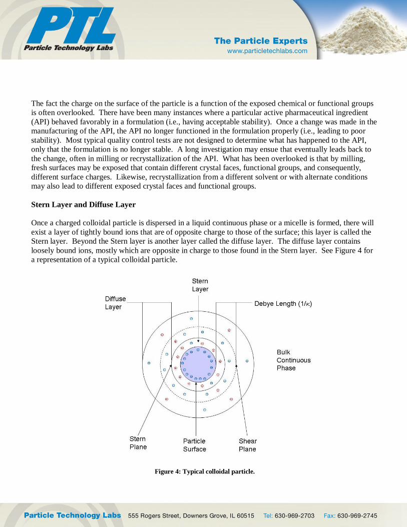
Stern Layer and Diffuse Layer

Once a charged colloidal particle is dispersed in a liquid continuous phase or a micelle is formed, there will

exist a layer of tightly bound ions that are of opposite charge to those of the surface; this layer is called the

Stern layer. Beyond the Stern layer is another layer called the diffuse layer. The diffuse layer contains

loosely bound ions, mostly which are opposite in charge to those found in the Stern layer. See Figure 4 for

a representation of a typical colloidal particle.

Figure 4: Typical colloidal particle.

Shear Plane

When a dispersed colloidal particle is exposed to an electric field, the particle, closely bound Stern layer,

and a portion of the loosely-bound diffuse layer will be attracted (or repelled) to or from the poles of the

field depending on the charge of the particle. Because the diffuse layer is only loosely bound, a portion of

the layer will move with the particle and a portion will not, creating a plane of shear. This is called the

shear plane or is sometimes referred to as the slip plane. It is at the shear plane where the electrophoretic

mobility is measured and the zeta potential is determined. The Stern layer and portion of the loosely bound

diffuse layer is sometimes referred to as the electrical double layer. The thickness of the double layer is

called the Debye length, and is given the symbol, 1/.

COLLOIDAL STABILITY

The stability and properties of colloidal systems have been studied for decades by a variety of individuals

(22-40). Colloids have also been modeled using a variety of approaches and for a variety of geometric

configurations including flat plates, cylinders, and spheres. Most of the mathematics and intricacies are

beyond the scope of this article, but some of the concepts require further explanation.

At the core of understanding colloidal stability are two opposing forces: Van der Waals attractions and

electrostatic repulsion. Van der Waals forces arise from atomic and molecular level interactions due to

induced and permanent dipoles in the system. They include Keesom interactions (i.e., from permanent

dipole/permanent dipole interactions), Debye interactions (i.e., from permanent dipole/induced dipole

interactions), and London interactions (i.e., from induced dipole/induced dipole interactions). They are

always attractive (negative in sign), are relatively weak, and are relatively long ranged.

The electrostatic repulsive forces are generally Coulombic in origin, are relatively strong, and are relatively

short ranged. In this case, they are also repulsive (i.e., positive in sign). Much more detail on all the forces

can be found in Israelachvili (1991) (14).

In order for a colloidal system to be stable, the repulsive forces between the particles must be greater than

the attractive forces. A typical potential energy plot vs. interparticle distance is given in Figure 5.

Interparticle Distance

Po

ten

tial

20 Min.

Ea

10 Min.

Figure 5: Potential energy diagram as a function of interparticle distance.

Figure 5 indicates a few features of note. In order from the right (greatest interparticle distance), it is shown

that at infinite distance, the potential between the particles approaches zero. As the particles approach each

other and the interparticle distance decreases, there exists a potential secondary minimum (20 min.) in

certain systems. Particles that enter the secondary minimum are weakly bound and are said to be

agglomerated or flocculated. The floccs, if present, are very loosely bound with an open structure and low

particle packing fraction. Flocculation is generally reversible with a small amount of required energy. Note

the secondary minimum is often quite broad and shallow.

As the particles approach closer, the repulsive forces manifest themselves in an energetic barrier or

activation energy, Ea. If this barrier is large enough, the particles will remain in or near their secondary

energetic minimum due to kinetics. However, if the particles come close enough to one another to

overcome the repulsive barrier, they will descend into the thermodynamic primary minimum (10 min.).

Particles that enter the primary minimum are strongly bound and are said to be aggregated. The aggregates

are tightly bound with a dense structure and high particle packing fraction. Aggregation is normally

considered an irreversible process.

At the other extreme end of the plot, where the interparticle distance approaches zero, the energetic

potential drastically increases as the particles begin to experience nuclear repulsion.

IMPORTANT FACTORS IN COLLOIDAL STABILITY

Given the plot in Figure 5, one might expect the most efficient manner to develop a highly stable colloidal

system would be to increase the energetic barrier, Ea, which prevents the particles from experiencing

irreversible aggregation at the primary energetic minimum. A list of significant factors that affect colloidal

stability can be derived through examination of the various theories. This list of factors generally includes

pH, ionic strength or conductivity, and temperature.

Temperature

Of these, temperature may be the easiest to conceptualize. As is the case with all chemical reactions, the

degree to which a reaction proceeds as a function of time is dependent on thermodynamics and kinetics (41-

43). In general, as the temperature of a reaction increases, so does the available energy, kT, and the

subsequent kinetic rate. Thus, one might expect the relative proportion of particles that are able to

overcome the energetic barrier to increase with an increase in temperature. Of course, temperature also

affects the Brownian motion of the particle and the dynamic viscosity of the liquid continuous phase (7, 44).

This is why colloidal measurements are often conducted at very controlled temperatures.

pH

Another very important factor is pH. As previously mentioned, one of the major sources of surface charge

is the dissociation of surface groups. An example of this mechanism would be protonation or deprotonation

of a particular functional group at the particle surface. Like a zwitterion, many surfaces can adopt a

negative or positive charge, depending on the pH. This, in turn, can lead to a negative or positive zeta

potential, the magnitude of which may be a function of pH.

Debye Length and Ionic Strength

Finally, 1/, called the Debye length, approximates the double layer thickness, where NA = Avogadro’s

number, z = ionic valence, M = concentration of each ion in the system, = dielectric constant, kB =

Boltzmann’s constant, and T = temperature.

Tk

MzNe

B

i

iiA

222000

[Equation 2]

As shown by Equation 2, as the ionic strength increases, the Debye length decreases. This effectively

increases the shielding effect of the double layer, thus decreasing the measured zeta potential. In fact, at a

given ionic strength called the critical coagulation concentration, most colloids can be forced to undergo

catastrophic instability, which is sometimes called “salting out” of the system.

Another interesting property of colloids comes from the equation for the ionic strength, I.

i

ii MzI 2 [Equation 3]

As shown, the ionic strength is a factor of the ionic valence squared. Thus, monovalent ions such as Na+1

,

K+1

, Cl-1

, and Br-1

contribute to the ionic strength as a function of their respective concentrations. However,

even trace levels of polyvalent ions such as Mg+2

, Ca+2

, and Al+3

can increase the ionic strength of the

system disproportionately and cause colloidal instability. It is for this reason why many wastewater

treatment facilities use FeCl3 as a flocculant (45).

ZETA POTENTIAL AND ELECTROPHORETIC MOBILITY

Electrokinetic effects may be defined as those phenomena involving tangential fluid motion adjacent to a

charged surface. There are a few electrokinetic effects often considered in colloidal systems:

electrophoresis, electro-osmosis, streaming potential, sedimentation potential, and electrokinetic sonic

amplitude. The majority of commercial instrumentation for the determination of zeta potential utilizes the

principle of electrophoresis.

Electrophoresis

Electrophoresis is defined as the movement of charged colloidal particles under the influence of an external

electric field. The electrophoretic velocity, e (m s–1

), is the velocity during electrophoresis. The

electrophoretic mobility, ue (m2 V

–1 s

–1), is the magnitude of the velocity divided by the magnitude of the

electric field strength.

Once the electrophoretic mobility, ue, has been measured, several mathematical equations may be used to

relate it to the zeta potential, . The proper equation is determined by first evaluating r, where 1/ is the

Debye length and r is radius of the particle or micelle. Once r is determined, the initial zeta potential is

calculated. Using the initial zeta potential determination, further refinements, or alternate equations may be

used as shown in the flowchart of Figure 6.

Figure 6: Zeta potential flowchart.

If r is large, say >20, then the Debye length is generally small. This is common in many aqueous systems.

If the absolute value of the initial measured zeta potential, |ξ|, is ≤ 50 mV, then it can be assumed the diffuse

layer is not conductive. In this case, the equation is called the Helmholtz-Smoluchowski equation [Equation

4]. is the dielectric constant and is the dynamic viscosity of the system.

eu [Equation 4]

Note the dependence of the electrophoretic mobility on the dielectric constant and viscosity. ue is directly

proportional to , so in aqueous systems where is very high (80.1 @ 200C), ue is typically very high.

Conversely, in organic systems such as methanol where is very low (30 @ 200C), ue is typically low.

Likewise, ue is indirectly proportional to , so in aqueous systems where is very low (1.002 cP @ 200C),

ue is typically very high and vice versa. It is for this reason that many commercial instruments have

difficulty measuring zeta potential on systems whose dynamic viscosity is greater than about 10 to 20 cP.

If the absolute value of the initial measured zeta potential is ≥ 50 mV, then the diffuse layer cannot be

assumed to be non-conductive and should be taken into account by using the O’Brien-White equation

[Equation 5] (46).

22222222

2222333332321

24

2ln42ln42ln82ln8

rzDezeDeTkez

zeDekTzDeTkeTkrzeDee

u

kT

ez

kT

ez

kT

ez

kT

ez

kT

ez

kT

ez

e

[Equation 5]

z is the electrolyte valence, is the zeta potential, k is Boltzmann’s constant, T is the absolute temperature,

D is the ionic diffusion rate, r is the radius of particle or micelle, is the viscosity, 1/ is the Debye length,

and is the diluent dielectric constant.

If r is small, say <1, then the Debye length is generally large. This is typical of many non-aqueous

systems. It may also hold true for aqueous systems with very low ionic strength. In this case, the Debye-

Hückel equation [Equation 6] should be used.

3

2eu [Equation 6]

If r is >1 but <20, then the Debye length is a moderate size, which is perhaps the most common scenario

for aqueous systems that have also have an average ionic strength. If the absolute value of the initial

measured zeta potential is ≤ 50 mV, then it can be assumed the diffuse layer is not conductive. In this case,

the preferred equation is called Henry’s equation [Equation 7]. Note Henry’s equation is a generalized

equation such that if r = , then as approaches 0, f () approaches 1, and Henry’s equation reduces to the

Debye-Hückel equation. Likewise, as approaches , f () approaches 3/2, and Henry’s equation reduces

to the Helmholtz-Smoluchowski equation.

fue

3

2 [Equation 7]

If the absolute value of the initial measured zeta potential is ≥ 50 mV, then the diffuse layer cannot be

assumed to be non-conductive and should be taken into account by using Oshima’s equation [Equation 8]

(47). In Equation 7, Kp is a factor to compensate for the conductivity of the diffuse layer. As can be seen,

Henry’s equation and Oshima’s equation are very similar and in the limit that the diffuse layer becomes

non-conductive, Oshima’s equation does reduce to Henry’s equation.

pe Kfu ,3

2

[Equation 8]

SAMPLE PREPARATION

A frequently asked question in this field is, “what is the zeta potential of my dry powder sample?”

This is a very difficult question to answer because by definition, a dry powder sample does not have a zeta

potential. The dry powder sample cannot establish an electrical double layer until it is dispersed in a

continuous liquid phase; thus, there is no electrophoretic mobility to measure and no zeta potential to

determine. This raises the issue of sample preparation.

As previously mentioned, the stability of a colloidal system is dependent on a number of factors. Some of

these include pH, ionic strength, and temperature. These must be closely monitored when making a

colloidal dispersion. One thing that is often ignored is the “history” of the dispersion. In many systems, the

colloid “remembers” its history. Though the explanation and fields of rheology and fluid dynamics are

beyond the scope of this paper, it is important to note the type, amount, and duration of sheer applied to the

colloidal system. For instance, a sonic bath may not yield the same product as a sonic probe. Likewise, a

small-scale blender batch may not yield the same product as a full-scale industrial mixer. Not only are the

sheer profiles different, but the time of application and in many cases, the resulting temperature levels, are

different if not controlled.

It is often important to note the concentration or volume fraction of the particles during the dispersion

process. The process history (i.e., if the dispersion has undergone filtration, centrifugation, or dilution) is

also important. Some colloidal systems are sensitive to ionic radii. NaCl may not behave the same as KCl

in certain systems because of the mismatched difference between the ionic radii of Na+1

(1.16Å) and K+1

(1.52Å) and that of Cl-1

(1.67Å) (48). The age of the dispersion may also make a difference in the zeta

potential determination, especially if the colloidal particle experiences ripening. Storage conditions,

especially temperature conditions, may drastically affect a colloid. All these may have an effect on the

resulting zeta potential determination and colloidal stability.

When dealing with colloidal systems, it is often necessary to dilute them in order to obtain particle size or

zeta potential determinations. This is because many instruments that measure zeta potential do so through

use of electrophoretic light scattering. Thus, some colloidal systems have to be diluted in order to minimize

multiple particle light scattering events. When a colloidal system is ultracentrifuged to separate the particles

from the continuous phase, the supernatant still contains the same concentration and type of ions as the

parent dispersion. The supernatant, called the “mother liquor”, may be used as the preferred diluent for the

parent dispersion. In this way, the volume fraction of solids may be reduced without changing the

electrolyte background.

Consideration of all the above factors needs to occur prior to sample preparation when performing zeta

potential determination. This is especially true if comparison between data sets is the end goal.

ZETA POTENTIAL DETERMINATION

When measuring zeta potential, a few limitations must be considered. Zeta potential cannot be measured on

a particle that is anchored to a substrate or locked in place by a solid continuous phase. The colloidal

particle must be free to move. In addition, the particle must have a large enough charge and small enough

size to move at a detectable rate when exposed to an electric potential. The upper limit on mean particle

diameter for which zeta potential may be measured is dependent on several factors, but in general, is

between 1 to 10 m.

There are several ways to measure zeta potential. Modern instrumentation primarily utilizes two principles:

electrophoretic light scattering and electrokinetic sonic amplitude (ESA). Electrophoretic light scattering

can be further divided into those methods that measure the resulting change in frequency and those methods

that measure the resulting change in phase.

Electrophoretic Light Scattering

When measuring zeta potential by electrophoretic light scattering, a dispersion is placed in a cell that has a

pair of electrodes at a fixed and known distance apart. A potential is then applied across the electrodes.

The colloidal particles will migrate to or away from the electrodes, and the direction and velocity will

depend on the charge of the particle and its environment. When a coherent incident light such as that from a

laser strikes the particle and is scattered, there is a change in the frequency and phase of the scattered light.

If the change in frequency is utilized, then a Fourier transform of the data is utilized to convert the data from

frequency domain to time domain. Once the data are expressed as a function of time, the velocity,

electrophoretic mobility, and subsequent zeta potential can be calculated. If the change in phase is utilized,

the determination is called phase analysis light scattering (PALS). In the case of PALS, the data are

expressed as a function of phase, which is already a function of time. Thus, a Fourier transform is not

necessary and the velocity, electrophoretic mobility, and subsequent zeta potential can be calculated with

greater ease, less computational requirement, and with greater sensitivity.

Electrokinetic Sonic Amplitude

When utilizing ESA, a dispersion is placed in a cell that has a pair of electrodes at a fixed and known

distance apart. An alternating current is then applied across the electrodes. When an alternating current

propagates through a colloidal dispersion, it causes the particles to vibrate in a way that depends on their

size and on their zeta potential at the frequency of the applied field. If there is a density difference between

the particles and the liquid, this motion will generate an acoustic wave of the same frequency as the applied

electric field (49-53). The sound wave is then detected by a very sensitive piezoelectric detector.

The ESA amplitude can then be used to calculate the electrophoretic mobility and zeta potential in a similar

manner as that for the other electrokinetic effects using Equation 9. ESA is the electrokinetic sonic

amplitude, is the viscosity, is the dielectric constant, is the volume fraction, is the difference in

density between the particle and the diluent, c is the speed of sound in the diluent, and G (a)-1

is a factor to

take into account the inertial forces of the particles at high frequency.

1

aG

c

ESA

[Equation 9]

ISOELECTRIC POINT DETERMINATION

A common measurement that is often associated with zeta potential determination is the isoelectric point

determination. The definition of the isoelectric point is the pH at which the electrophoretic mobility is zero.

As previously mentioned, a colloidal dispersion is considered stable if the magnitude of the zeta potential is

large, and this is typically desired. However, there are some cases where it is desired for the dispersion to

be unstable. A colloidal system is generally least stable at its isoelectric point.

In order to determine the isoelectric point, the most common method is to measure the zeta potential of a

colloidal system over a wide range of pH values. The pH values are normally adjusted by the addition of an

acid or base in a typical pH titration manner. For example, as the pH of a particle with –OH surface groups

is decreased, the degree of protonization will increase, yielding a net positive charge on the surface and a

positive zeta potential. The opposite is also true. As the pH is increased, the degree of deprotonization will

increase, yielding a net negative charge on the surface and a negative zeta potential. Remember the zeta

potential is not the surface potential, but rather the potential measured at the shear plane, which is a function

of the surface charge as well as all the other factors mentioned earlier. The isoelectric point, like the zeta

potential, is not only dependent on the surface charge and other factors, but is also sometimes useful in

determining purity of the colloidal particle as well as giving insight into the history of the particle. An

isoelectric point titration for a typical colloidal system is shown (as the red data) in Figure 7.

Figure 7: Zeta potential titration of a common colloid before and after heat treatment.

-50

-40

-30

-20

-10

0

10

0 2 4 6 8 10 12

pH

Zeta

Po

ten

tia

l (m

V)

Sample as received Sample after heat treatment

Like all zeta potential determinations, the isoelectric point determination is sensitive to the history of the

colloidal system. A specific example has been observed due to the processing temperature of a colloidal

sample. In this example, the sample was produced in a pyrogenic process and calcined for a given time at a

given temperature. The sample was then analyzed and the data are presented in Table III. Afterwards, the

same batch of material was further heat treated under a nitrogen blanket, the surface annealed, and several –

OH groups were lost in a condensation mechanism. This heat-treated sample was then analyzed and the

data are presented in Table III. The isoelectric point titration for the heat-treated material is shown (as the

blue data) in Figure 7. Clearly, the two colloidal particles were different because of their temperature

histories and one would expect them to behave quite differently in a variety of applications.

Table III: Isoelectric point of pre- and post-heat treated material.

B.E.T. Surface

Area (m2/g)

Mean

Diameter

(nm)

Zeta Potential

@ pH 10 (mV)

Isoelectric

Point

(pH)

As received 200 200 -45 2.0

Post heat treatment 70 200 -15 4.5

The process of properly titrating a system is not intuitive to most. A common mistake is to disperse a

colloid at a given pH such as at pH 7. The pH of the dispersion is then decreased in increments to perhaps

pH 1 as the zeta potential is measured. Then, the chemist erroneously titrates the dispersion up to pH 10,

while taking zeta potential determinations. There are at least two striking errors in this methodology: the

history of the system is ignored, and the effect on the zeta potential is not only due to the pH of the system,

but is also due to the increase in ionic strength.

In the case of the first error, if the effect of conductivity is ignored, there is still the effect of the change in

pH on the surface chemistry of the particle. As the pH decreases, this may affect the solubility of the

surface. It may also affect the surface energy and distribution of functional groups, similar to how

temperature and annealing affected the surface in the previous example. These changes to the surface are

often irreversible. In fact, it is not uncommon to titrate a system down in pH while taking zeta potential

determinations, then as the chemist titrates the pH back up, the zeta potential determinations do not agree

with the initial determinations due to the irreversible changes on the particle surface. It is usually better to

split the original dispersion then use one-half to titrate down and the other half to titrate up. For an example

of this type of titration error, see Figure 8. In Figure 8, the red data represent the first part of the titration

when the pH is decreased. The blue data represent the second part of the titration when the pH is increased.

Note the hysteresis between the two data sets.

-50

-40

-30

-20

-10

0

10

20

0 2 4 6 8 10 12

pH

Zeta

Po

ten

tial

(mV

)

Figure 8: Zeta potential titration of a colloidal system as it is commonly (and erroneously) performed.

In the case of the second error, that of the differences in conductivity, there are two typical ways to

overcome the error. One way is to disperse the sample in a continuous medium that has a relatively high

ionic strength such as 0.1 M KCl. In this way, the change in conductivity due to the increase in ions from

the acid or base is overwhelmed by the ionic strength of the diluent. This is definitely the easiest way to

overcome the error, but due to the dependency of the zeta potential determination on conductivity, it may

not be the most accurate.

An alternate method to overcome the conductivity error is to proceed as follows:

1. Using an aliquot of the prepared dispersion, adjust the pH to the maximum level required

(i.e., pH 2 or pH 10).

2. Measure the conductivity at both ends of the pH range and determine which pH level

yields the dispersion with the highest conductivity.

3. Using a fresh aliquot of the prepared dispersion, titrate the dispersion either up or down

with base or acid, respectively. Concurrently, perform a conductivity titration by adding a

dilute spectator ion such as KCl to the dispersion. The endpoint of each conductivity

titration should be the highest conductivity measured in step 2.

4. Using another fresh aliquot of the prepared dispersion, titrate the dispersion the opposite

pH direction with base or acid. Concurrently, perform a conductivity titration by adding a

dilute spectator ion such as KCl to the dispersion. The endpoint of each conductivity

titration should be the highest conductivity measured in step 2.

This methodology separates the history of increasing pH from that of decreasing pH. It also compensates

for the change in conductivity due to pH titration, which effectively deconvolves the effects of pH from

conductivity on the isoelectric point.

CONCLUSIONS

When requesting or measuring zeta potential, there are many factors that should or must be taken into

consideration, some of which include the following:

pH. Colloidal stability and the isoelectric point must be considered.

Conductivity or ionic strength. Do not exceed the critical coagulation concentration (unless

desired).

Temperature. Excess temperature in either direction can destabilize a suspension.

Particle size. The particles or micelles must be free to move and need to be small enough that they

have a measureable electrophoretic mobility.

Solubility (or lack thereof). Ensure the sample is a dispersion, not a solution.

Viscosity of the diluents. Excessive viscosity can attenuate the electrophoretic mobility.

Debye length and initial zeta potential. These are used to determine the proper equation to calculate

zeta potential from electrophoretic mobility.

History. This includes shear history, storage conditions, dilution, centrifugation, and filtration.

There is clearly a need for regulatory guidance in the international pharmacopeias. In the interim, there are

draft ISO standards, textbooks, and numerous research papers that can be used and referenced.

REFERENCES

1. ASTM standard, D4187-82, Zeta Potential of Colloids in Water and Waste Water, 1982.

2. ISO draft standard 13099-1, Methods for Zeta Potential Determination — Part 1: Introduction,

2010.

3. ISO draft standard 13099-2, Methods for Zeta Potential Determination — Part 2: Optical methods,

2010.

4. ISO standard 13099-3, Methods for Zeta Potential Determination — Part 3: Acoustic methods, (not

released at the time of this publication).

5. Measurement and Interpretation of Electrokinetic Phenomena, (IUPAC Technical Report), Pure

Appl. Chem., 77, 10, p. 1753, 2005.

6. Hiemenz, P.C., Rajagopalan, R., Principles of Colloid and Surface Chemistry, 3rd

edition, Dekker,

1997.

7. Einstein, A., Investigations in the Theory of Brownian Movement, Dover, 1956.

8. Allen, T., Particle Size Measurement Volume 1 – Powder Sampling and Particle Size Measurement,

5th

edition, Chapman & Hall, 1997.

9. ISO standard 14887, Sample Preparation – Dispersing Procedures for Powder in Liquids, 2000.

10. Iler, R.K., The Chemistry of Silica – Solubility, Polymerization, Colloidal and Surface Properties,

and Biochemistry, John Wiley & Sons, 1978.

11. Ostwald, W., Z. Phys. Chem. 37, p. 385, 1901.

12. Baldan, A., J. Mat. Sci., 37, p. 2171, 2002.

13. Kreuter, J., Colloidal Drug Delivery Systems (Drugs and the Pharmaceutical Sciences), CRC Press,

1st edition, 1994.

14. Israelachvili, J. N., Intermodular and Surface Forces, 2nd

edition, Academic Press, 1991.

15. Loeb, A.L., Overbeek, J.Th.G. and Wiersema, P.H., The Electrical Double Layer around a

Spherical Particle, M.I.T. Press, 1961.

16. Hunter, R.J., Foundations of Colloid Science, 2nd

edition, Oxford University Press, 2001.

17. Good, R.J., Surface and Colloid Science, Vol. 11, Plenum, 1979.

18. Ross, S. and Morrison, I.D., Colloidal Systems and Interfaces, Wiley, 1988.

19. Attard, P., Adv. Chem. Phys., 92, 1, 1996.

20. Lyklema J., Fundamentals of Interface and Colloid Science, Elsevier Publishing Company, 1991.

21. Shaw, D., Introduction to Colloid and Surface Chemistry, 4th edition, Butterworth-Heinemann,

1992.

22. Faraday, M., Philos. Trans. R. Soc. London, 1857.

23. Schulze, H., Journal für Praktische Chemie, 27, 1, p. 320, 1883.

24. Chapman, S., Philos. Trans. R. Soc. London, Series A, Containing Papers of a Mathematical or

Physical Character, 211, 1912.

25. Gouy, M., J. de Phys., 4, 9, 1910; Gouy, M., J. de Phys., 5, 1, 1911; Gouy, M., J. de Phys., 14, 1,

1920.

26. Smoluchowski, M., Z. Phys. Chem. 92, p. 129, 1917.

27. Debye, P. & Hückel, E., Physikalische Zeitschrift, 24, p. 185, 1923.

28. Stern, O., Zeit. Elektrochem., 1924.

29. London, F., Zeit. Physik. Chem. B., 1930.

30. Kallmann, H. & Willstaetter, M., Naturwissenschaften, 20, 51, p. 952, 1932.

31. Hamaker, H.C., Physica, 4, p. 1058, 1937.

32. Derjaguin, B.V. & Landau, L., Acta Physiochim. URSS, 14, p. 633, 1941.

33. Verway, E.J.W. & Overbeek, J. Th. G., Theory of the Stability of Lyophobic Colloids, Elsevier,

1948.

34. Derjaguin, B.V., Abricossova, I.I. and Lifshitz, E.M., Q. Rev. Chem. Soc., 10, p. 295, 1956;

Derjaguin, B.V., Sci. Am., 3, 1960.

35. Dzyaloshinskii, I.E., Lifshitz, E.M., and Pitaevskii, L.P., Sov. Phys. Usp., 4, p. 153, 1961.

36. F.M. Fowkes, Ind. Eng. Chem. 56, 40, 1964.

37. Sonntag, H. & Strenge, K., Coagulation and Stability of Disperse Systems, Halsted, 1964.

38. Gregory, J., Adv. Colloid Interface Sci., 2, p. 396, 1969.

39. Dukhin, S.S. & Semenikhin, N.M. Koll. Zhur., 32, p. 366, 1970.

40. Hunter, R.J., Zeta Potentials in Colloid Science: Principles and Applications, Academic Press, 1981.

41. Adamson, A., Physical Chemistry of Surfaces, 6th edition, John Wiley & Sons, 1997.

42. Atkins, P. & De Paula, J., Physical Chemistry, 9th edition, W.H. Freeman, 2009.

43. Steinfeld, J., Francisco, J., Hase, W., Chemical Kinetics and Dynamics, 2nd

edition, Prentice Hall,

1998.

44. Larson, R., The Structure and Rheology of Complex Fluids (Topics in Chemical Engineering),

Oxford University Press, 1998.

45. Bratby, J., Coagulation and Flocculation in Water and Wastewater Treatment, 2nd

edition, IWA

Publishing, 2006.

46. O’Brien, R.W. & White, L.R., J. Chem. Soc., Faraday Trans. II, 74, p. 1607, 1978.

47. Oshima, H., J. Colloid Interface Sci., 168, p. 269, 1994.

48. Shannon, R.D., Acta Cryst., A32, p. 751, 1976.

49. O'Brien, R.W., Midmore, B., Lamb, A. and Hunter, R.J., Faraday Discuss. Chem. Soc., 90, 1990.

50. O’Brien, R.W., J. Fluid Mech., 190, 71, 1988.

51. Debye, P., Trans. Faraday Soc., 30, 1934.

52. Bell, G. & Levine, S., Trans. Faraday Soc., 54, 1958.

53. Freeman, M., Method and Apparatus for Measuring a Colloidal Potential , United States Patent,

4,552,019, NOV 12, 1985.