ZEISS EVO SOP

May 2017

ELECTRON OPTICS

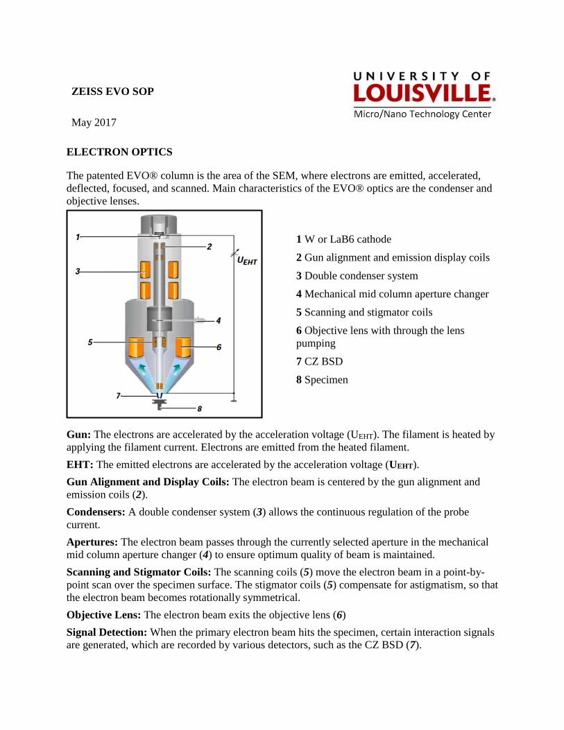
The patented EVO® column is the area of the SEM, where electrons are emitted, accelerated,

deflected, focused, and scanned. Main characteristics of the EVO® optics are the condenser and

objective lenses.

1 W or LaB6 cathode

2 Gun alignment and emission display coils

3 Double condenser system

4 Mechanical mid column aperture changer

5 Scanning and stigmator coils

6 Objective lens with through the lens

pumping

7 CZ BSD

8 Specimen

Gun: The electrons are accelerated by the acceleration voltage (UEHT). The filament is heated by

applying the filament current. Electrons are emitted from the heated filament.

EHT: The emitted electrons are accelerated by the acceleration voltage (UEHT).

Gun Alignment and Display Coils: The electron beam is centered by the gun alignment and

emission coils (2).

Condensers: A double condenser system (3) allows the continuous regulation of the probe

current.

Apertures: The electron beam passes through the currently selected aperture in the mechanical

mid column aperture changer (4) to ensure optimum quality of beam is maintained.

Scanning and Stigmator Coils: The scanning coils (5) move the electron beam in a point-by-

point scan over the specimen surface. The stigmator coils (5) compensate for astigmatism, so that

the electron beam becomes rotationally symmetrical.

Objective Lens: The electron beam exits the objective lens (6)

Signal Detection: When the primary electron beam hits the specimen, certain interaction signals

are generated, which are recorded by various detectors, such as the CZ BSD (7).

SIGNAL DETECTION

The interaction products most frequently used for the generation of images in scanning electron

microscopy are secondary electrons (SE) and backscattered electrons (BSE).

Standard detectors Detected signals Typical application

SE2 detector

(Everhart-Thornley) SE2 Topography and surface structure

VPSE detector SE On VP systems only

Optional detectors Detected signals Typical application

Backscattered electron

detectors, including 4-

quadrant CZBSD

BSE

Topographical (crystal orientation),

atomic number contrast.

Cathodoluminescence (CL)

detector Light photons Mineralogy

Scanning Transmission

Electron Microscopy

(STEM) detector

Transmission

electrons

Transmission imaging of thin

sections in biological and

mineralogical examinations

EPSE (needle and ring)

SE*

*By means of

measuring current

produced by

ionization of gas by

SE Electrons

generated around

Extended pressure applications.

Typically when imaging biological

specimens in a fully hydrated form

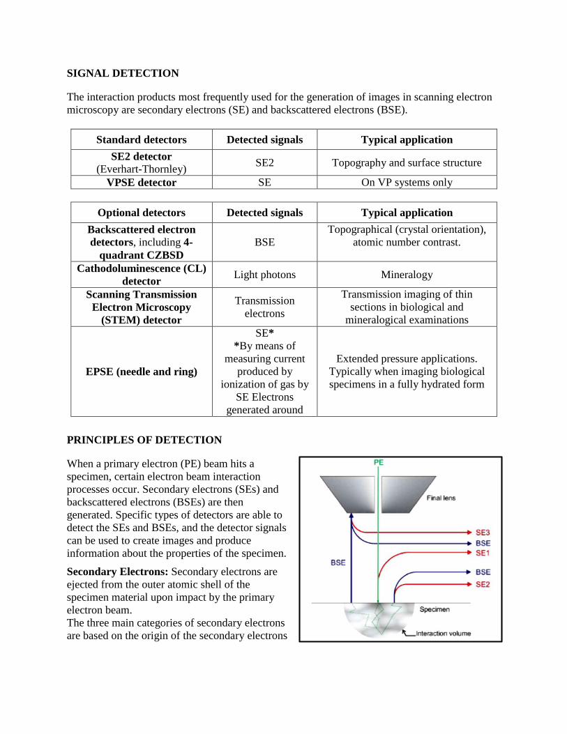
PRINCIPLES OF DETECTION

When a primary electron (PE) beam hits a

specimen, certain electron beam interaction

processes occur. Secondary electrons (SEs) and

backscattered electrons (BSEs) are then

generated. Specific types of detectors are able to

detect the SEs and BSEs, and the detector signals

can be used to create images and produce

information about the properties of the specimen.

Secondary Electrons: Secondary electrons are

ejected from the outer atomic shell of the

specimen material upon impact by the primary

electron beam.

The three main categories of secondary electrons

are based on the origin of the secondary electrons

and on the distance from the PE impact point, where they leave the specimen.

SE1 electrons are generated and leave the surface of the specimen directly at the spot where

the primary electron beam impacts on the specimen surface.

SE2 electrons are generated after multiple scattering inside the interaction volume, and leave

the specimen at a greater distance from the primary beam’s impact point.

SE3 electrons are generated by backscattered electrons colliding with the chamber walls or

the lens system. Secondary electrons have low energy (less than 50 eV).

Backscatter Electrons: All electrons with energy higher than 50 eV are known as backscattered

electrons (BSEs).

BSEs are generated by elastic scattering in a much deeper range of the interaction volume and

carry depth information.

The backscatter coefficient increases with increasing atomic number of the elements within the

specimen. This allows the BSE detector to generate atomic number contrast, or compositional

contrast images.

ET-SE DETECTOR (SE2 DETECTOR)

The ET-SE, or Everhart-Thornley, detector is mounted on the wall of the specimen chamber, and

is therefore classed as a ‘chamber detector’. Due to its position in the chamber, the SE2 detector

views the specimen laterally.

The SE2 detector allows detection of secondary electrons with a small backscattered component.

Secondary electrons moving towards the detector are attracted by the collector and are directed

towards the scintillator accelerated by the scintillator voltage.

Operating Principle

When the high energy electrons hit the scintillator layer (2), photons are generated inside the

scintillator. These photons are directed out of the vacuum system through a light pipe (3) and are

transferred to the photomultiplier (5). The photomultiplier multiplies the flashes of light and

outputs a signal that can be used for imaging.

Collector Bias Voltage

The Detectors tab of the SEM Control panel allows you to adjust the collector bias voltage in the

range –250 V to +400 V in steps of 1 V. This voltage generates a bias in front of the detector.

The bias attracts the low energy SE electrons and accelerates them towards the detector. For all

standard applications the collector bias voltage is usually set to 300 V.

It is also possible to set the collector bias voltage to a negative value. This generates a field that

deflects the secondary electrons, preventing them from reaching the scintillator and contributing

to the signal. Backscattered electrons are not affected significantly by the negative bias voltage

and reach the scintillator to contribute to image information. This allows the generation of a

‘pseudo- backscattered image’, which shows enhanced topographical information.

Surface images that show enhanced topographical information can also be generated using BSE

detectors, but they do not show the shadows that can be created using the SE2 detector.

When using a positive collector bias voltage, surfaces that are tilted in the direction of the

detector are emphasized, but there are no shadowing effects.

When using a negative collector bias voltage, the image shows enhanced topographical

contrast, which arises mainly from the extreme shadowing effects. However, the fine surface

details are less visible.

Applications

The SE2 detector can be used in the complete high-voltage range.

The working distance has a significant effect on the efficiency of the SE2 detector. Shadowing

effects occur when the working distance is too short and, if the specimen is too close to the final

lens, most of the electrons will be deflected by the field of the electrostatic lens or move to the

final lens itself. This means they cannot be detected by the SE2 detector.

Depending on the specimen material and on the specimen geometry, a minimum working

distance of approximately 4 mm should be used. Extreme signal loss is likely to occur if shorter

working distances than this are used. Conversely, the SE2 detector is very good when used for

imaging at long working distances. This is particularly important for low magnification imaging

that is necessary for adjusting the orientation of the specimen holder or locating a specific area

on the specimen.

Optimal initial settings

The following settings provide a good field of view for navigating on the specimen at low

magnifications:

Initial working distance in the range 10 mm to 20 mm.

Acceleration voltage of approximately 10 kV.

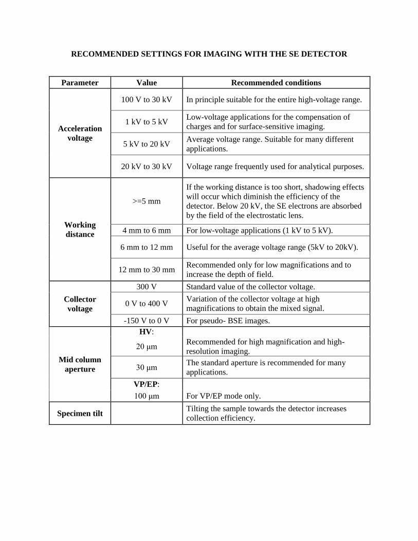
RECOMMENDED SETTINGS FOR IMAGING WITH THE SE DETECTOR

Parameter Value Recommended conditions

Acceleration

voltage

100 V to 30 kV In principle suitable for the entire high-voltage range.

1 kV to 5 kV Low-voltage applications for the compensation of

charges and for surface-sensitive imaging.

5 kV to 20 kV Average voltage range. Suitable for many different

applications.

20 kV to 30 kV Voltage range frequently used for analytical purposes.

Working

distance

>=5 mm

If the working distance is too short, shadowing effects

will occur which diminish the efficiency of the

detector. Below 20 kV, the SE electrons are absorbed

by the field of the electrostatic lens.

4 mm to 6 mm For low-voltage applications (1 kV to 5 kV).

6 mm to 12 mm Useful for the average voltage range (5kV to 20kV).

12 mm to 30 mm Recommended only for low magnifications and to

increase the depth of field.

Collector

voltage

300 V Standard value of the collector voltage.

0 V to 400 V Variation of the collector voltage at high

magnifications to obtain the mixed signal.

-150 V to 0 V For pseudo- BSE images.

Mid column

aperture

HV:

20 μm Recommended for high magnification and high-

resolution imaging.

30 μm The standard aperture is recommended for many

applications.

VP/EP:

100 μm For VP/EP mode only.

Specimen tilt Tilting the sample towards the detector increases

collection efficiency.

OPERATION PROCEDURE

!!! Log into the tool by using FOM, it will turn on the monitor.

1. Login to Zeiss Computer, choose SEM user, PW guest

2. Start SMART SEM USER INTERFACE Software .

3. Login to software [User: your SEM user ID, Password: your SEM password].

EM Server will automatically start up.

Preparing the specimen holder

IMPORTANT

Contamination caused by fingerprints can lead to vacuum deterioration or prolonged pumping

times. Always wear lint-free gloves when touching specimen, specimen holder or stage.

1. Attach the specimen to the stub by using conductive carbon, adhesive metal or carbon tape.

Ensure that the specimen area to be analyzed is in good contact with the stub. This will ensure

high electrical conductivity between the specimen and the stub.

2. Use the tweezers to insert the stub into the specimen holder.

3. Use the Allen key to tighten the location screw and secure the specimen.

Loading the specimen chamber

1. Click the TV icon in the toolbar or press the Camera button on the keyboard.

CAUTION: Risk of damaging the objective lens and/or your specimen Ensure not to hit the

objective lens while driving the stage. Change to TV mode to observe the moving stage.

2. Select Tools/Goto Control Panel from the menu, the SEM Control panel opens.

3. Go to the Vacuum tab and click VENT to vent the specimen chamber. The same can be

achieved by left-click on VAC indicator in the status bar and click VENT.

4. A message appears asking: ’Are you sure you want to vent?’ Confirm by clicking on YES.

5. When vented slowly open the chamber door.

IMPORTANT: Keep the chamber door open as short as possible.

All specimen holders are fitted with a dovetail fitting so that the position of the specimen holder

is exactly defined.

6. Mount the specimen holder:

a. Make sure that you place the dovetail fitting in the correct orientation onto the holding

device on the specimen stage.

b. Make sure that the flat side of the dovetail fitting of the specimen holder is flush with the

milled edge of the stage.

7. When closing the chamber door check the chamber scope to ensure the specimen does not hit

any components when it is introduced into the specimen chamber.

8. Carefully close the chamber door and click Pump in the SEM Control panel. The same can be

achieved by left-click on VAC indicator in the status bar and click PUMP.

Locating the Specimen

1. Move the specimen by using the dual joystick or by calling the Soft Joystick via Tools/Goto

Panel/Soft Joystick.

2. Carefully move the specimen closer to the objective lens. The distance between objective lens

and specimen surface should be less than about 10 mm.

Switching on the Gun

1. In the Vacuum tab: Check that EHT Vac ready=Yes is indicated. Alternatively, check that

there is a green tick alongside VAC in the status bar.

2. Click GUN in the status bar and select Beam On from the pop-up menu. The gun is being run

up.

Switching on the EHT

Note: ’EHT’ stands for Extra High Tension. This voltage has to be applied to the gun in order to

make it emit electrons.

1. Watch the vacuum status messages on the Vacuum tab of the SEM Control panel. When the

required vacuum has been reached you will see the message Vac Status = Ready.

2. Go to the Gun tab and set the acceleration voltage: a move the EHT Target slider to the

desired value. Alternatively click EHT Target = and type in the desired value.

3. Switch on the EHT:

a. Click EHT in the status bar.

b. Select EHT On from the pop-up menu. The EHT will run up to the target value.

The status bar buttons are merged and the ALL : button appears. Now, the electron beam is

on.

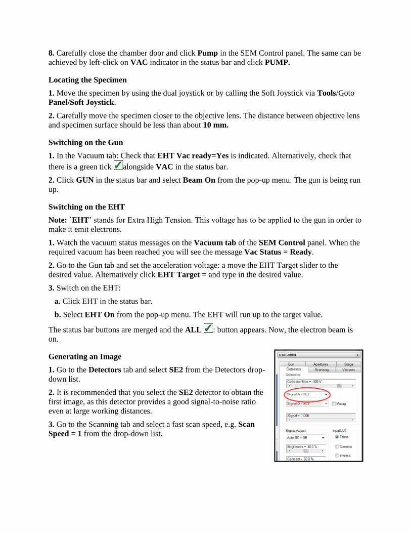
Generating an Image

1. Go to the Detectors tab and select SE2 from the Detectors drop-

down list.

2. It is recommended that you select the SE2 detector to obtain the

first image, as this detector provides a good signal-to-noise ratio

even at large working distances.

3. Go to the Scanning tab and select a fast scan speed, e.g. Scan

Speed = 1 from the drop-down list.

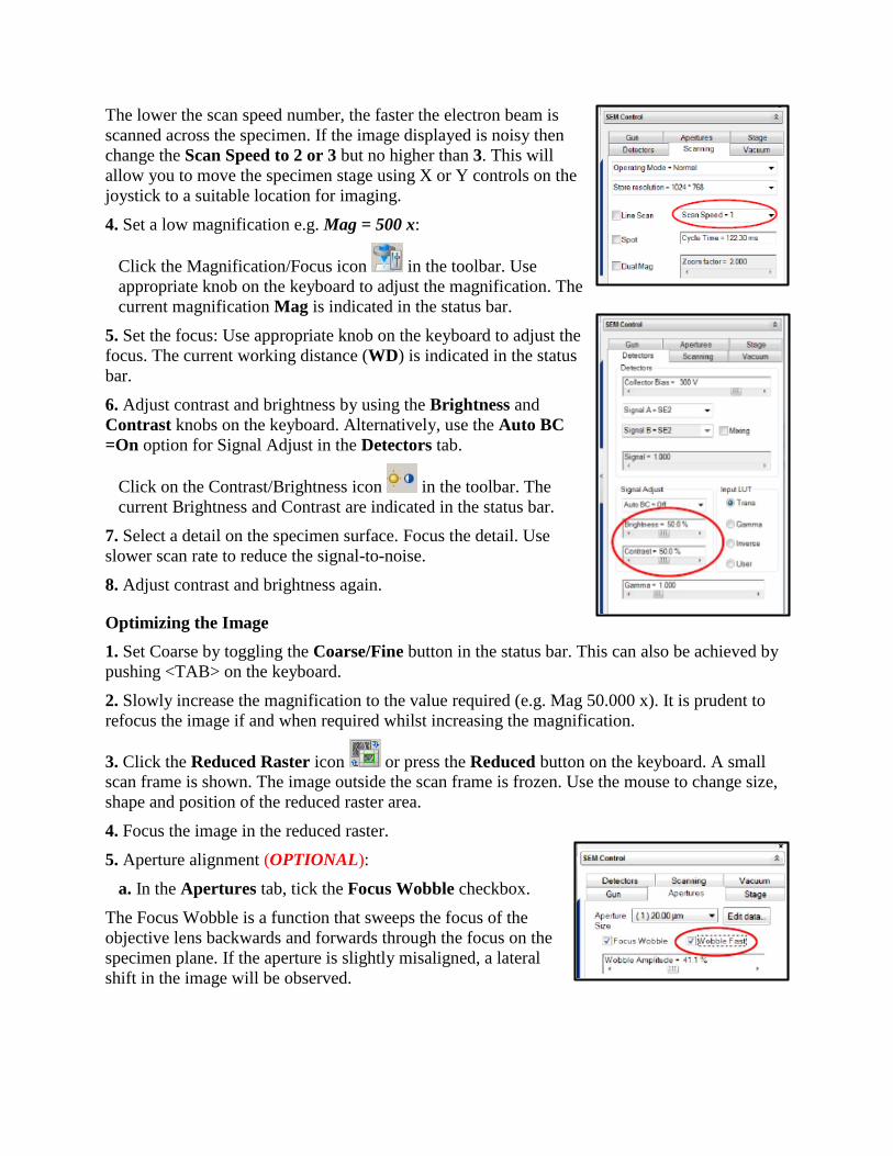
The lower the scan speed number, the faster the electron beam is

scanned across the specimen. If the image displayed is noisy then

change the Scan Speed to 2 or 3 but no higher than 3. This will

allow you to move the specimen stage using X or Y controls on the

joystick to a suitable location for imaging.

4. Set a low magnification e.g. Mag = 500 x:

Click the Magnification/Focus icon in the toolbar. Use

appropriate knob on the keyboard to adjust the magnification. The

current magnification Mag is indicated in the status bar.

5. Set the focus: Use appropriate knob on the keyboard to adjust the

focus. The current working distance (WD) is indicated in the status

bar.

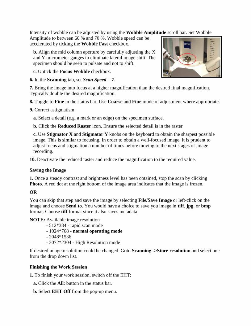
6. Adjust contrast and brightness by using the Brightness and

Contrast knobs on the keyboard. Alternatively, use the Auto BC

=On option for Signal Adjust in the Detectors tab.

Click on the Contrast/Brightness icon in the toolbar. The

current Brightness and Contrast are indicated in the status bar.

7. Select a detail on the specimen surface. Focus the detail. Use

slower scan rate to reduce the signal-to-noise.

8. Adjust contrast and brightness again.

Optimizing the Image

1. Set Coarse by toggling the Coarse/Fine button in the status bar. This can also be achieved by

pushing <TAB> on the keyboard.

2. Slowly increase the magnification to the value required (e.g. Mag 50.000 x). It is prudent to

refocus the image if and when required whilst increasing the magnification.

3. Click the Reduced Raster icon or press the Reduced button on the keyboard. A small

scan frame is shown. The image outside the scan frame is frozen. Use the mouse to change size,

shape and position of the reduced raster area.

4. Focus the image in the reduced raster.

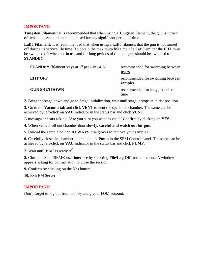
5. Aperture alignment (OPTIONAL):

a. In the Apertures tab, tick the Focus Wobble checkbox.

The Focus Wobble is a function that sweeps the focus of the

objective lens backwards and forwards through the focus on the

specimen plane. If the aperture is slightly misaligned, a lateral

shift in the image will be observed.

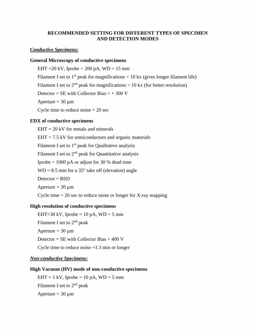
Intensity of wobble can be adjusted by using the Wobble Amplitude scroll bar. Set Wobble

Amplitude to between 60 % and 70 %. Wobble speed can be

accelerated by ticking the Wobble Fast checkbox.

b. Align the mid column aperture by carefully adjusting the X

and Y micrometer gauges to eliminate lateral image shift. The

specimen should be seen to pulsate and not to shift.

c. Untick the Focus Wobble checkbox.

6. In the Scanning tab, set Scan Speed = 7.

7. Bring the image into focus at a higher magnification than the desired final magnification.

Typically double the desired magnification.

8. Toggle to Fine in the status bar. Use Coarse and Fine mode of adjustment where appropriate.

9. Correct astigmatism:

a. Select a detail (e.g. a mark or an edge) on the specimen surface.

b. Click the Reduced Raster icon. Ensure the selected detail is in the raster

c. Use Stigmator X and Stigmator Y knobs on the keyboard to obtain the sharpest possible

image. This is similar to focusing. In order to obtain a well-focused image, it is prudent to

adjust focus and stigmation a number of times before moving to the next stages of image

recording.

10. Deactivate the reduced raster and reduce the magnification to the required value.

Saving the Image

1. Once a steady contrast and brightness level has been obtained, stop the scan by clicking

Photo. A red dot at the right bottom of the image area indicates that the image is frozen.

OR

You can skip that step and save the image by selecting File/Save Image or left-click on the

image and choose Send to. You would have a choice to save you image in tiff, jpg, or bmp

format. Choose tiff format since it also saves metadata.

NOTE: Available image resolution

- 512*384 - rapid scan mode

- 1024*768 - normal operating mode

- 2048*1536

- 3072*2304 - High Resolution mode

If desired image resolution could be changed. Goto Scanning ->Store resolution and select one

from the drop down list.

Finishing the Work Session

1. To finish your work session, switch off the EHT:

a. Click the All: button in the status bar.

b. Select EHT Off from the pop-up menu.

IMPORTANT:

Tungsten Filament: It is recommended that when using a Tungsten filament, the gun is turned

off when the system is not being used for any significant period of time.

LaB6 Filament: It is recommended that when using a LaB6 filament that the gun is not turned

off during its service life time. To obtain the maximum life time of a LaB6 emitter the EHT must

be switched off when not in use and for long periods of time the gun should be switched to

STANDBY.

STANDBY (filament stays at 1st peak I=1.4 A) recommended for switching between

users

EHT OFF recommended for switching between

samples

GUN SHUTDOWN recommended for long periods of

time

2. Bring the stage down and go to Stage Initialization, wait until stage is stops at initial position.

3. Go to the Vacuum tab and click VENT to vent the specimen chamber. The same can be

achieved by left-click on VAC indicator in the status bar and click VENT.

A message appears asking: ’Are you sure you want to vent?’ Confirm by clicking on YES.

4. When vented roll out chamber door slowly, careful and watch out for gun.

5. Unload the sample holder. ALWAYS, use gloves to remove your samples.

6. Carefully close the chamber door and click Pump in the SEM Control panel. The same can be

achieved by left-click on VAC indicator in the status bar and click PUMP.

7. Wait until VAC is ready .

8. Close the SmartSEM® user interface by selecting File/Log Off from the menu. A window

appears asking for confirmation to close the session.

9. Confirm by clicking on the Yes button.

10. Exit EM Server.

IMPORTANT:

Don’t forget to log out from tool by using your FOM account.

RECOMMENDED SETTING FOR DIFFERENT TYPES OF SPECIMEN

AND DETECTION MODES

Conductive Specimens:

General Microscopy of conductive specimens

EHT =20 kV, Iprobe = 200 pA, WD = 15 mm

Filament I set to 1st peak for magnifications < 10 kx (gives longer filament life)

Filament I set to 2nd peak for magnifications > 10 kx (for better resolution)

Detector = SE with Collector Bias > + 300 V

Aperture = 30 µm

Cycle time to reduce noise = 20 sec

EDX of conductive specimens

EHT = 20 kV for metals and minerals

EHT = 7.5 kV for semiconductors and organic materials

Filament I set to 1st peak for Qualitative analysis

Filament I set to 2nd peak for Quantitative analysis

Iprobe = 1000 pA or adjust for 30 % dead time

WD = 8.5 mm for a 35° take off (elevation) angle

Detector = BSD

Aperture = 30 µm

Cycle time = 20 sec to reduce noise or longer for X-ray mapping

High resolution of conductive specimens

EHT=30 kV, Iprobe = 10 pA, WD = 5 mm

Filament I set to 2nd peak

Aperture = 30 µm

Detector = SE with Collector Bias + 400 V

Cycle time to reduce noise =1.3 min or longer

Non-conductive Specimens:

High Vacuum (HV) mode of non-conductive specimens

EHT = 1 kV, Iprobe = 10 pA, WD = 5 rnm

Filament I set to 2nd peak

Aperture = 30 µm

Detector = SE with Collector Bias + 400 V

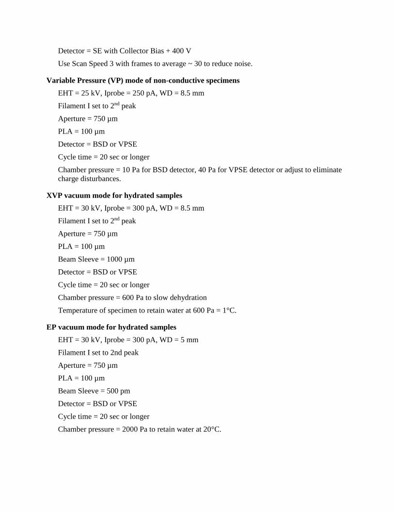
Use Scan Speed 3 with frames to average ~ 30 to reduce noise.

Variable Pressure (VP) mode of non-conductive specimens

EHT = 25 kV, Iprobe = 250 pA, WD = 8.5 mm

Filament I set to 2nd peak

Aperture = 750 µm

PLA = 100 µm

Detector = BSD or VPSE

Cycle time = 20 sec or longer

Chamber pressure = 10 Pa for BSD detector, 40 Pa for VPSE detector or adjust to eliminate

charge disturbances.

XVP vacuum mode for hydrated samples

EHT = 30 kV, Iprobe = 300 pA, WD = 8.5 mm

Filament I set to 2nd peak

Aperture = 750 µm

PLA = 100 µm

Beam Sleeve = 1000 µm

Detector = BSD or VPSE

Cycle time = 20 sec or longer

Chamber pressure = 600 Pa to slow dehydration

Temperature of specimen to retain water at 600 Pa = 1°C.

EP vacuum mode for hydrated samples

EHT = 30 kV, Iprobe = 300 pA, WD = 5 mm

Filament I set to 2nd peak

Aperture = 750 µm

PLA = 100 µm

Beam Sleeve = 500 pm

Detector = BSD or VPSE

Cycle time = 20 sec or longer

Chamber pressure = 2000 Pa to retain water at 20°C.

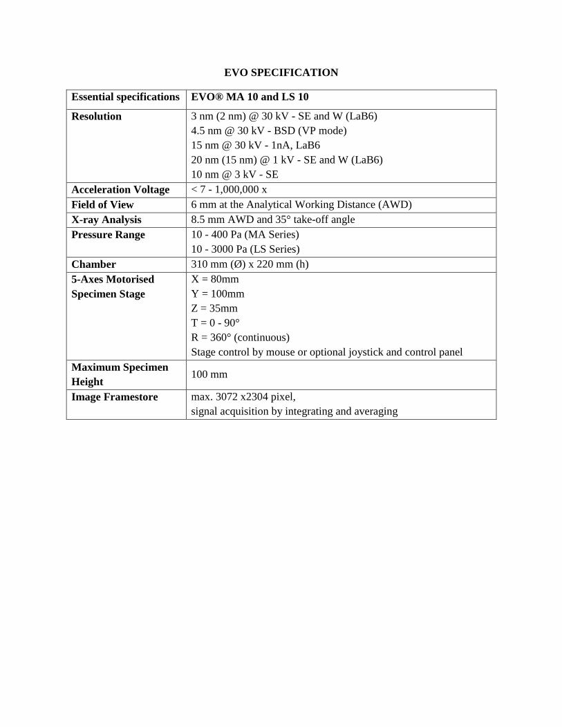
EVO SPECIFICATION

Essential specifications EVO® MA 10 and LS 10

Resolution 3 nm (2 nm) @ 30 kV - SE and W (LaB6)

4.5 nm @ 30 kV - BSD (VP mode)

15 nm @ 30 kV - 1nA, LaB6

20 nm (15 nm) @ 1 kV - SE and W (LaB6)

10 nm @ 3 kV - SE

Acceleration Voltage < 7 - 1,000,000 x

Field of View 6 mm at the Analytical Working Distance (AWD)

X-ray Analysis 8.5 mm AWD and 35° take-off angle

Pressure Range 10 - 400 Pa (MA Series)

10 - 3000 Pa (LS Series)

Chamber 310 mm (Ø) x 220 mm (h)

5-Axes Motorised

Specimen Stage

X = 80mm

Y = 100mm

Z = 35mm

T = 0 - 90°

R = 360° (continuous)

Stage control by mouse or optional joystick and control panel

Maximum Specimen

Height 100 mm

Image Framestore max. 3072 x2304 pixel,

signal acquisition by integrating and averaging