zabalza, jaime and ren, jinchang and ren, jie and liu, zhe ... · jaime zabalza,1 jinchang ren,1,*...

Zabalza, Jaime and Ren, Jinchang and Ren, Jie and Liu, Zhe and

Marshall, Stephen (2014) Structured covariance principal component

analysis for real-time onsite feature extraction and dimensionality

reduction in hyperspectral imaging. Applied Optics, 53 (20). pp. 4440-

4449. ISSN 1559-128X , http://dx.doi.org/10.1364/AO.53.004440

This version is available at https://strathprints.strath.ac.uk/48907/

Strathprints is designed to allow users to access the research output of the University of

Strathclyde. Unless otherwise explicitly stated on the manuscript, Copyright © and Moral Rights

for the papers on this site are retained by the individual authors and/or other copyright owners.

Please check the manuscript for details of any other licences that may have been applied. You

may not engage in further distribution of the material for any profitmaking activities or any

commercial gain. You may freely distribute both the url (https://strathprints.strath.ac.uk/) and the

content of this paper for research or private study, educational, or not-for-profit purposes without

prior permission or charge.

Any correspondence concerning this service should be sent to the Strathprints administrator:

[email protected]

The Strathprints institutional repository (https://strathprints.strath.ac.uk) is a digital archive of University of Strathclyde research

outputs. It has been developed to disseminate open access research outputs, expose data about those outputs, and enable the

management and persistent access to Strathclyde's intellectual output.

http://strathprints.strath.ac.uk/

mailto:[email protected]

http://strathprints.strath.ac.uk/

Structured covariance principal component analysis for

real-time onsite feature extraction and dimensionality

reduction in hyperspectral imaging

Jaime Zabalza,1 Jinchang Ren,1,* Jie Ren,2 Zhe Liu,3 and Stephen Marshall1

1Centre for Excellence in Signal and Image Processing, Department of Electronic and Electrical Engineering,

University of Strathclyde, Glasgow, UK

2College of Electronics and Information, Xi’an Polytechnic University, Xi’an, China

3Department of Applied Mathematics, Northwestern Polytechnical University, Xi’an, China

*Corresponding author: [email protected]

Received 13 March 2014; revised 27 May 2014; accepted 28 May 2014;

posted 3 June 2014 (Doc. ID 208226); published 4 July 2014

Presented in a three-dimensional structure called a hypercube, hyperspectral imaging suffers from alarge volume of data and high computational cost for data analysis. To overcome such drawbacks, prin-cipal component analysis (PCA) has been widely applied for feature extraction and dimensionality re-duction. However, a severe bottleneck is how to compute the PCA covariance matrix efficiently and avoidcomputational difficulties, especially when the spatial dimension of the hypercube is large. In this paper,structured covariance PCA (SC-PCA) is proposed for fast computation of the covariance matrix. In linewith how spectral data is acquired in either the push-broom or tunable filter method, different imple-mentation schemes of SC-PCA are presented. As the proposed SC-PCA can determine the covariancematrix from partial covariance matrices in parallel even without prior deduction of the mean vector,it facilitates real-time data analysis while the hypercube is acquired. This has significantly reducedthe scale of required memory and also allows efficient onsite feature extraction and data reduction tobenefit subsequent tasks in coding and compression, transmission, and analytics of hyperspectraldata. © 2014 Optical Society of AmericaOCIS codes: (100.4145) Motion, hyperspectral image processing; (100.2960) Image analysis.http://dx.doi.org/10.1364/AO.53.004440

1. Introduction

Hyperspectral imaging (HSI), through capturing datafrom numerous and contiguous spectral bands, hasprovided a unique and invaluable solution for a num-ber of application areas. Due to the large spectralrange covered includingnot only visible light, likenor-mal imagingdevices, but also (near) infraredandevenultraviolet, HSI is able to detect and identify theminute differences of objects and even their changesin terms of temperature and moisture. Consequently,

HSI is able to address traditional applications inremote sensing, mining, agriculture, geology, andmilitary surveillance aswell asmanynewly emerginglab-based data analyses. These new applications canbe easily found in security, food quality analysis, andmedical and pharmaceutical fields as well as counter-feit goods and documents detection [1–6].

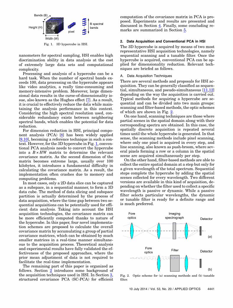
In HSI, as shown in Fig. 1, the captured data formsa three-dimensional (3D) structure, namely a hyper-cube, including a 2D spatial measurement and aspectral dimension. As a result, the total data con-tained can be indexed as HWB, where each of thesymbols refers to the height, width, and bands of thehypercube, respectively. With the narrow band in

1559-128X/14/204440-10$15.00/0© 2014 Optical Society of America

4440 APPLIED OPTICS / Vol. 53, No. 20 / 10 July 2014

http://dx.doi.org/10.1364/AO.53.004440

nanometers for spectral sampling, HSI enables highdiscrimination ability in data analysis at the costof extremely large data sets and computationalcomplexity.

Processing and analysis of a hypercube can be ahard task. When the number of spectral bands ex-ceeds 100, data processing on the hypercube appearslike video analytics, a really time-consuming andmemory-intensive problem. Moreover, large dimen-sional data results in the curse-of-dimensionality is-sue, also known as the Hughes effect [7]. As a result,it is crucial to effectively reduce the data while main-taining the analysis performance in this context.Considering the high spectral resolution used, con-siderable redundancy exists between neighboringspectral bands, which enables the potential for datareduction.

For dimension reduction in HSI, principal compo-nent analysis (PCA) [8] has been widely applied[9,10], becoming a reference technique in such a con-text. However, for the 3D hypercube in Fig. 1, conven-tional PCA analysis needs to convert the hypercubeinto a B ×HW matrix to determine the relevantcovariance matrix. As the second dimension of thematrix becomes extreme large, usually over 100kilobytes, it introduces a fundamental difficulty incalculating the covariance matrix. As a result, theimplementation often crashes due to memory andcomputing problems.

In most cases, only a 2D data slice can be capturedas a subspace, in a sequential manner, to form a 3Ddata cube. The method of data slicing and subspacepartition is actually determined by the process ofdata acquisition, where the time gap between two se-quential acquisitions can be potentially used for effi-cient data analysis. Taking into account the HSIacquisition technologies, the covariance matrix canbe more efficiently computed thanks to nature ofthe hypercube. In this paper, four novel implementa-tion schemes are proposed to calculate the overallcovariance matrix by accumulating a group of partialcovariance matrices, which can be obtained by muchsmaller matrices in a real-time manner simultane-ous to the acquisition process. Theoretical analysisand experimental results have fully validated the ef-fectiveness of the proposed approaches, where theprior mean adjustment of data is not required tofacilitate the real-time implementation.

The remaining part of this paper is organized asfollows. Section 2 introduces some background ofthe acquisition techniques used in HSI. In Section 3,structured covariance PCA (SC-PCA) for efficient

computation of the covariance matrix in PCA is pro-posed. Experiments and results are presented anddiscussed in Section 4. Finally, some concluding re-marks are summarized in Section 5.

2. Data Acquisition and Conventional PCA in HSI

The 3D hypercube is acquired by means of two mostrepresentative HSI acquisition technologies, namelysequential scanning and a tunable filter. Once thehypercube is acquired, conventional PCA can be ap-plied for dimensionality reduction. Relevant tech-niques are briefed as follows.

A. Data Acquisition Techniques

There are several methods and proposals for HSI ac-quisition. They can be generally classified as sequen-tial, simultaneous, and pseudo-simultaneous [11,12]depending on the way the acquisition is carried out.Typical methods for acquiring a hypercube are se-quential and can be divided into two main groups:scanning and filter-based methods, the optic schemesof which are shown in Fig. 2.

On one hand, scanning techniques are those wherepartial scenes in the spatial domain along with theircorresponding spectra are obtained. In this case, thespatially discrete acquisition is repeated severaltimes until the whole hypercube is generated. In thatsense, the scanning methods include pixel scanning,where only one pixel is acquired in every step, andline scanning, also known as push-broom, where sev-eral pixels forming a row or a column in the spatialscene are acquired simultaneously per step.

On the other hand, filter-based methods are able tocollect the entire spatial domain at a step but only fora given wavelength of the total spectrum. Sequentialsteps complete the hypercube by adding the spatialscenes collected for every wavelength. Two differentversions are available in this kind of acquisition, de-pending on whether the filter used to collect a specificwavelength is passive or dynamic. While a passivefilter selects particular wavelengths, the dynamicor tunable filter is ready for a definite range andis much preferred.

Fig. 1. 3D hypercube in HSI.

Fig. 2. Optic scheme for (a) scanning methods and (b) tunablefilter.

10 July 2014 / Vol. 53, No. 20 / APPLIED OPTICS 4441

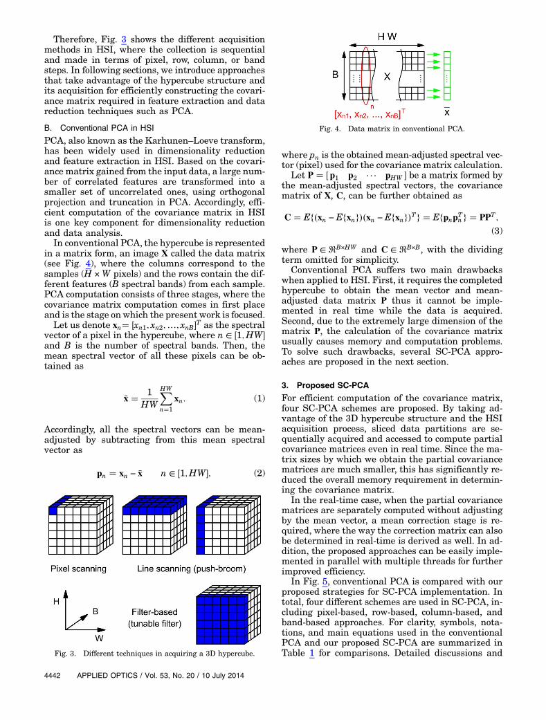
Therefore, Fig. 3 shows the different acquisitionmethods in HSI, where the collection is sequentialand made in terms of pixel, row, column, or bandsteps. In following sections, we introduce approachesthat take advantage of the hypercube structure andits acquisition for efficiently constructing the covari-ance matrix required in feature extraction and datareduction techniques such as PCA.

B. Conventional PCA in HSI

PCA, also known as the Karhunen–Loeve transform,has been widely used in dimensionality reductionand feature extraction in HSI. Based on the covari-ance matrix gained from the input data, a large num-ber of correlated features are transformed into asmaller set of uncorrelated ones, using orthogonalprojection and truncation in PCA. Accordingly, effi-cient computation of the covariance matrix in HSIis one key component for dimensionality reductionand data analysis.

In conventional PCA, the hypercube is representedin a matrix form, an image X called the data matrix(see Fig. 4), where the columns correspond to thesamples (H ×W pixels) and the rows contain the dif-ferent features (B spectral bands) from each sample.PCA computation consists of three stages, where thecovariance matrix computation comes in first placeand is the stage on which the present work is focused.

Let us denote xn� �xn1; xn2;…; xnB�T as the spectral

vector of a pixel in the hypercube, where n ∈ �1; HW�and B is the number of spectral bands. Then, themean spectral vector of all these pixels can be ob-tained as

x̄ �1

HW

X

HW

n�1

xn: (1)

Accordingly, all the spectral vectors can be mean-adjusted by subtracting from this mean spectralvector as

pn � xn − x̄ n ∈ �1; HW�; (2)

where pn is the obtained mean-adjusted spectral vec-tor (pixel) used for the covariance matrix calculation.

Let P � � p1 p2 � � � pHW � be a matrix formed bythe mean-adjusted spectral vectors, the covariancematrix of X, C, can be further obtained as

C � Ef�xn − Efxng��xn − Efxng�Tg � Efpnp

Tn g � PPT ;

(3)

where P ∈ RB×HW and C ∈ RB×B, with the dividingterm omitted for simplicity.

Conventional PCA suffers two main drawbackswhen applied to HSI. First, it requires the completedhypercube to obtain the mean vector and mean-adjusted data matrix P thus it cannot be imple-mented in real time while the data is acquired.Second, due to the extremely large dimension of thematrix P, the calculation of the covariance matrixusually causes memory and computation problems.To solve such drawbacks, several SC-PCA appro-aches are proposed in the next section.

3. Proposed SC-PCA

For efficient computation of the covariance matrix,four SC-PCA schemes are proposed. By taking ad-vantage of the 3D hypercube structure and the HSIacquisition process, sliced data partitions are se-quentially acquired and accessed to compute partialcovariance matrices even in real time. Since the ma-trix sizes by which we obtain the partial covariancematrices are much smaller, this has significantly re-duced the overall memory requirement in determin-ing the covariance matrix.

In the real-time case, when the partial covariancematrices are separately computed without adjustingby the mean vector, a mean correction stage is re-quired, where the way the correction matrix can alsobe determined in real-time is derived as well. In ad-dition, the proposed approaches can be easily imple-mented in parallel with multiple threads for furtherimproved efficiency.

In Fig. 5, conventional PCA is compared with ourproposed strategies for SC-PCA implementation. Intotal, four different schemes are used in SC-PCA, in-cluding pixel-based, row-based, column-based, andband-based approaches. For clarity, symbols, nota-tions, and main equations used in the conventionalPCA and our proposed SC-PCA are summarized inTable 1 for comparisons. Detailed discussions andFig. 3. Different techniques in acquiring a 3D hypercube.

Fig. 4. Data matrix in conventional PCA.


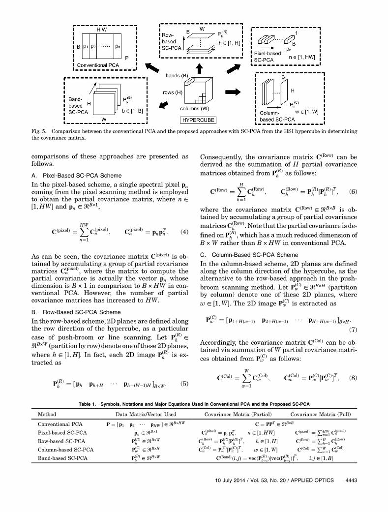
comparisons of these approaches are presented asfollows.

A. Pixel-Based SC-PCA Scheme

In the pixel-based scheme, a single spectral pixel pncoming from the pixel scanning method is employedto obtain the partial covariance matrix, where n ∈�1; HW� and pn ∈ RB×1,

C�pixel� �X

HW

n�1

C�pixel�n ; C

�pixel�n � pnp

Tn : (4)

As can be seen, the covariance matrix C�pixel� is ob-tained by accumulating a group of partial covariancematrices C

�pixel�n , where the matrix to compute the

partial covariance is actually the vector pn whosedimension is B × 1 in comparison to B ×HW in con-ventional PCA. However, the number of partialcovariance matrices has increased to HW.

B. Row-Based SC-PCA Scheme

In the row-based scheme, 2D planes are defined alongthe row direction of the hypercube, as a particular

case of push-broom or line scanning. Let P�R�h ∈

RB×W (partition by row) denote one of these 2Dplanes,

where h ∈ �1; H�. In fact, each 2D image P�R�h is ex-

tracted as

P�R�h � � ph ph�H � � � ph��W−1�H �B×W : (5)

Consequently, the covariance matrix C�Row� can bederived as the summation of H partial covariance

matrices obtained from P�R�h as follows:

C�Row� �X

H

h�1

C�Row�

h ; C�Row�

h � P�R�h �P

�R�h �

T; (6)

where the covariance matrix C�Row� ∈ RB×B is ob-tained by accumulating a group of partial covariance

matricesC�Row�

h . Note that the partial covariance is de-

fined on P�R�h , which has a much reduced dimension of

B ×W rather than B ×HW in conventional PCA.

C. Column-Based SC-PCA Scheme

In the column-based scheme, 2D planes are definedalong the column direction of the hypercube, as thealternative to the row-based approach in the push-

broom scanning method. Let P�C�w ∈ RB×H (partition

by column) denote one of these 2D planes, where

w ∈ �1;W�. The 2D image P�C�w is extracted as

P�C�w � �p1�H�w−1� p2�H�w−1� � � � pH�H�w−1� �B×H :

(7)

Accordingly, the covariance matrix C�Col� can be ob-tained via summation of W partial covariance matri-

ces obtained from P�C�w as follows:

C�Col� �X

W

w�1

C�Col�w ; C

�Col�w � P

�C�w �P

�C�w �

T; (8)

Fig. 5. Comparison between the conventional PCA and the proposed approaches with SC-PCA from the HSI hypercube in determiningthe covariance matrix.

Table 1. Symbols, Notations and Major Equations Used in Conventional PCA and the Proposed SC-PCA

Method Data Matrix/Vector Used Covariance Matrix (Partial) Covariance Matrix (Full)

Conventional PCA P � �p1 p2 � � � pHW � ∈ RB×HW C � PPT ∈ RB×B

Pixel-based SC-PCA pn ∈ RB×1 C�pixel�n � pnp

Tn ; n ∈ �1; HW� C�pixel� �

P

HWn�1

C�pixel�n

Row-based SC-PCA P�R�h ∈ RB×W C

�Row�

h � P�R�h �P

�R�h �

T; h ∈ �1;H� C�Row� �

P

Hh�1

C�Row�

h

Column-based SC-PCA P�C�w ∈ RB×H C

�Col�w � P

�C�w �P

�C�w �

T; w ∈ �1;W� C�Col� �

P

Ww�1

C�Col�w

Band-based SC-PCA P�B�b ∈ RH×W C�Band��i; j� � vec�P�B�

b�i��vec�P�B�b�j��

T; i; j ∈ �1; B�


where the partial covariance matrix is sized of B × B.Again the covariance matrix is obtained by accumu-

lating a group of partial covariance matrices C�Col�w ,

where the matrix to compute the partial covariancehas a much reduced dimension of B ×H rather thanB ×HW in conventional PCA.

D. Band-Based SC-PCA Scheme

Different from the abovementioned three SC-PCAapproaches, the band-based SC-PCA scheme is de-rived from a tunable-filter-based data acquisitionprocess, where all the spatial information is capturedfor a selected wavelength by tuning the optic part ofthe system. Let us define 2D planes along the band

direction of a hypercube as P�B�b ∈ RH×W (partition by

spectral band), where b ∈ �1; B�. The 2D image P�B�b

can be represented as

P�B�b �

2

6

6

4

p1�b� � � � pH�W−1��1�b�

.

.

...

....

pH�b� � � � pHW�b�

3

7

7

5

: (9)

Note that the selected data partition P�B�b contains

all pixels in only one specified spectral band ratherthan the whole spectrum. This fundamental differ-ence has led to the computation of partial covariancematrices, an impossible task as implemented inother SC-PCA approaches. As a result, element-based covariance matrix computation is employedas explained below.

For an element in position �i; j� of the final covari-ance matrix, we have that

C�Band��i; j� � vec�P�B�b�i��vec�P

�B�b�j��

T; (10)

where vec�� transforms the 2D plane P�B�b into a vec-

tor in R1×HW , resulting in a scalar value from themultiplication in Eq. (10). The overall covariance ma-trix is obtained by progressive inclusion of elements�i; j� derived from bands i and j, respectively, wherethe vectors to compute these elements have a muchreduced dimension of 1 ×HW rather than B ×HW inconventional PCA.

E. Mean Correction for Real-Time Computation

Note that the proposed schemes can be directly ap-plied on the whole hypercube when the data acquis-ition process is completed, which results in a muchreduced memory requirement in determining thecovariance matrix. However, the main idea here isto apply these approaches during the acquisitionstage for fast computation of the covariance matrixeven without parallel implementation, as suggestedin [13,14].

For simultaneous data acquisition and PCAprocessing, sequentially obtained partitions of dataare not mean-adjusted. As a result, instead of using

the partitions pn, P�R�h , and P

�C�w for pixel-, row-, and

column-based schemes, respectively, only the non-mean-adjusted equivalent partitions, namely xn,

X�R�h , and X

�C�w , can be used in these three real-time

implementation schemes. Note that in the band-based SC-PCA scheme the initial mean adjustmentin Eq. (2) is feasible as all pixel values from the samewavelength are available when sequentially col-lected band by band. As a result, the mean correctionis not needed for band-based SC-PCA.

Taking the pixel-based approach for example, se-quentially obtained pixels xn are not mean-adjustedas in the conventional PCA (1,2). Hence a correctionfactor M from the mean spectral vector x̄ in Eq. (1)must be applied:

pnpTn � xnx

Tn �M

�pixel�n M

�pixel�n � x̄ x̄T − xnx̄

T− x̄xTn ;

(11)

where M�pixel�n ∈ RB×B is made by the corresponding

pixel xn and x̄, and its construction can be easilyunderstood by thinking in terms of the product ofsubtracted values,

pn�i�pn�j� � �xn�i� − x̄�i��xn�j� − x̄�j��

� xn�i�xn�j� � x̄�i�x̄�j� − xn�i�x̄�j� − x̄�i�xn�j�:

(12)

Therefore, for real-time processing, the covariancematrix obtained by the pixel-based SC-PCA now is

C�pixel� �X

HW

n�1

xnxTn �

X

HW

n�1

M�pixel�n : (13)

In the row-based approach, a correction factor Mmust be applied again, similar to the pixel-basedcase:

P�R�h �P

�R�h �

T� X

�R�h �X

�R�h �

T�M

�R�h M

�R�h

� x̄ x̄T − X�R�h �x̄ � � � x̄�TB×W − �x̄ � � � x̄�B×W �X

�R�h �

T;

(14)

where M�R�h ∈ RB×B is made by the corresponding

partition or subspace X�R�h and x̄. Now the covariance

matrix is obtained, again adding the correction factorat the end of the acquisition:

C�Row� �X

H

h�1

X�R�h �X

�R�h �

T�

X

H

h�1

M�R�h : (15)

Analogously to the row-based approach, a correctionis added in the column-based case:


P�C�w �P

�C�w �

T� X

�C�w �X

�C�w �

T�M

�C�w M

�C�w

� x̄ x̄T − X�C�w �x̄ � � � x̄�TB×H − �x̄ � � � x̄�B×H �X

�C�w �

T;

(16)

where M�C�w ∈ RB×B is made by the corresponding

partition or subspace X�C�w and x̄. Finally, a similar

expression to the other cases but now using column-based partitions is achieved:

C�Col� �X

W

w�1

X�C�w �X

�C�w �

T�

X

W

w�1

M�C�w : (17)

The correction elements in Eqs. (13), (15), and (17)are in fact equivalent to each other and can be com-puted in the same way for these three approaches asa correction matrix CM ∈ RB×B:

CM �X

HW

n�1

M�pixel�n �

X

H

h�1

M�R�h �

X

W

w�1

M�C�w

�X

HW

n�1

�x̄ x̄T − xnx̄T− x̄xTn �: (18)

In addition, it is unnecessary to wait until the end ofthe acquisition process in order to start determiningthe correction matrix. Taking the pixel-based SC-PCA for example; an element �i; j� in the correctionmatrix CM can be expressed as

CM�i; j� �X

HW

n�1

x̄�i�x̄�j� −X

HW

n�1

xn�i�x̄�j� −X

HW

n�1

x̄�i�xn�j�

� HW�x̄�i�x̄�j�� − x̄�j�X

HW

n�1

xn�i� − x̄�i�X

HW

n�1

xn�j�;

(19)

where the second and third element, multiplying anddividing by the same factor, can be obtained as

x̄�j�HW1

HW

X

HW

n�1

xn�i� � x̄�j�HWx̄�i�

x̄�i�HW1

HW

X

HW

n�1

xn�j� � x̄�i�HWx̄�j�: (20)

Accordingly, we can further define correction matrixCM as

CM�i; j� � −HWx̄�i�x̄�j�: (21)

And finally, CM can be obtained by

CM�i; j� � −

1

HW

X

HW

n�1

xn�i�X

HW

n�1

xn�j�: (22)

As a result, elements in the correction matrix canbe obtained by accumulating the values in line withthe process when the data is acquired. Finally, thecovariance matrices in pixel-, row-, and column-based SC-PCA approaches can be, respectively,obtained by correction using CM as follows:

C�pixel� �X

HW

n�1

xnxTn � CM

C�Row� �X

H

h�1

X�R�h �X

�R�h �

T� CM

C�Col� �X

W

w�1

X�C�w �X

�C�w �

T� CM: (23)

F. Equivalency of the Approaches

It is worth noting that these four proposed strategiesare in fact equivalent to the conventional PCA. Belowwe will show how the pixel-based SC-PCA scheme isactually equal to the conventional PCA.

In conventional PCA, the covariance matrix C isdefined by C � PPT ∈ RB×B from Eq. (3). For eachelement �i; j�, it can be expressed as

C�i; j� �X

HW

n�1

pn�i�pn�j�: (24)

On the other hand, in the pixel-based approach, thepartial covariance matrix is determined by

C�pixel�n � pnp

Tn

�

2

6

6

4

pn�1�pn�1� � � � pn�1�pn�B�

.

.

...

....

pn�B�pn�1� � � � pn�B�pn�B�

3

7

7

5

B×B

: (25)

According to Eq. (4), the covariance matrix can beobtained by accumulating these partial covariancematrices as

C�pixel��X

HW

n�1

C�pixel�n

�

2

6

6

6

4

P

HWn�1

pn�1�pn�1� ��P

HWn�1

pn�1�pn�B�

.

.

...

....

P

HWn�1

pn�B�pn�1� ��P

HWn�1

pn�B�pn�B�

3

7

7

7

5

B×B

:

(26)

If we compare Eqs. (24) and (26), it is apparent thatthe pixel-based SC-PCA approach generates thesame covariance matrix as conventional PCA does;hence the two approaches are equivalent to eachother. Similar mechanisms can be also used to prove


the equivalency of the conventional PCA to other pro-posed SC-PCA approaches.

4. Experimental Results

The proposed approaches have been implementedusing Matlab, along with the conventional PCA, yetthe achieved results are independent of any specificprogramming language. With the extracted principalcomponents from various PCA schemes, a supportvector machine (SVM) takes them as input vectorsfor data classification.Corresponding results are thencompared to validate the effectiveness of theseSC-PCA schemes. Four stages of the experimentalsetup, including data description, data conditioning,feature extraction, and data classification, are dis-cussed in detail as follows, along with the results.

A. Data Description

The Airborne Visible/InfraRed Imaging Spectrom-eter (AVIRIS) is a sensor instrument widely usedby HSI researchers for data acquisition, deliveringcalibrated images in 224 contiguous bands with spec-tral wavelengths ranging from 400 to 2500 nm [15].Another well-known remote sensing instrument isthe Reflective Optics System Imaging Spectrometer(ROSIS), providing 114 bands with a spectral rangebetween 430 and 860 nm [16]. Finally HYPERION,aboard the EO-1 spacecraft, is able to provide sceneswith more than 200 spectral bands in the range 400–2500 nm from on-orbit missions [17]. Using the abovethree sensors, three publicly available data sets withdefined ground truth [18] are used in our experi-ments for quantitative performance evaluation.

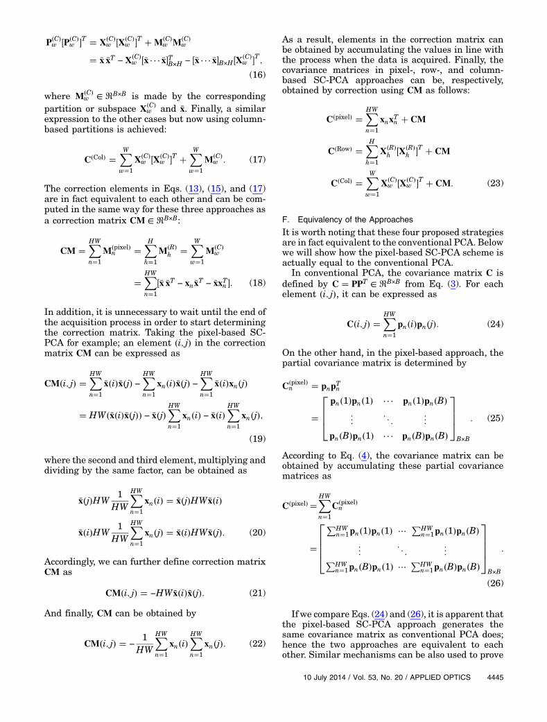
First, the AVIRIS Indian Pines data set, as shownin Fig. 6, was collected over an agricultural study sitein northwest Indiana in United States. The image ismade of 145 × 145 pixelswith 220 spectral reflectancebands in the wavelength range 400–2500 nm. Thisdata set is for land usage evaluation purpose, wheresixteen land cover classes are labeled in the image,presenting mostly agriculture, forest, and perennialvegetation.

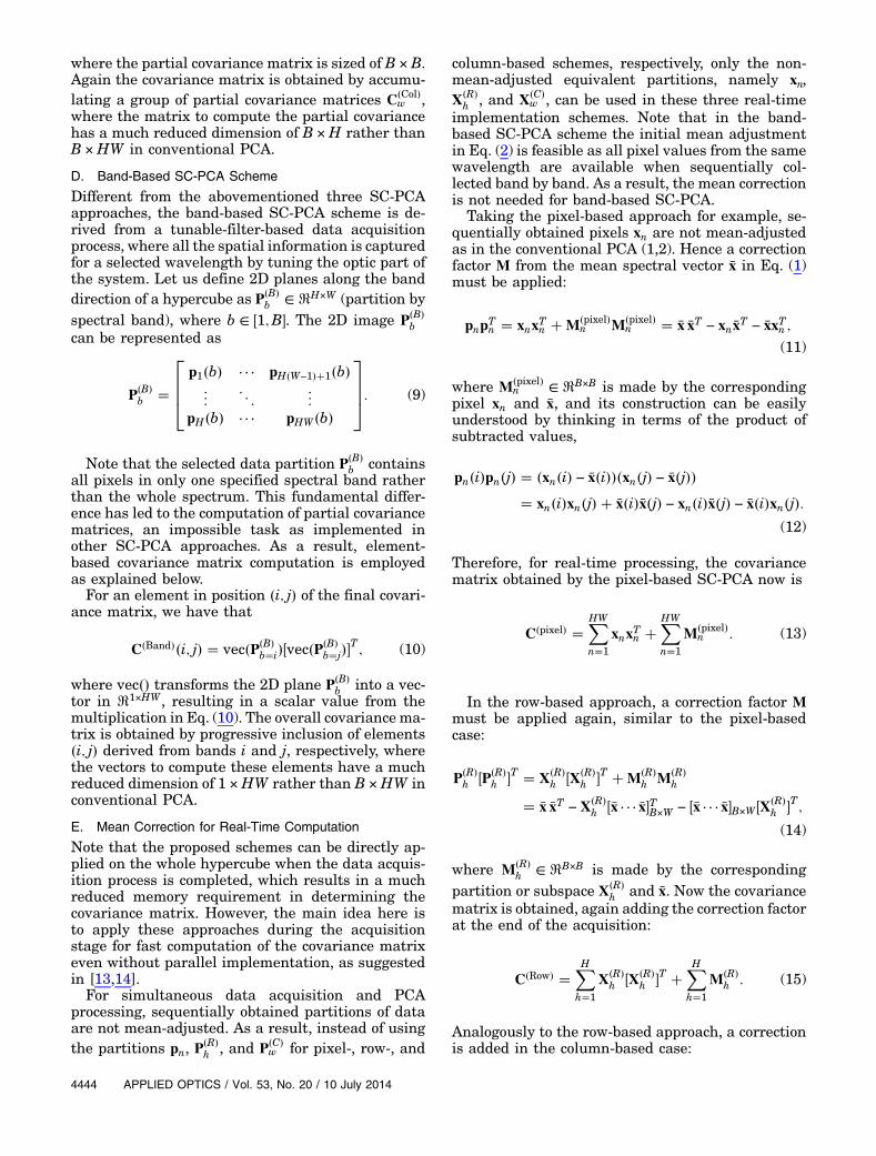
Second, the ROSIS Pavia University A data set(Pavia UA, shown in Fig. 7), corresponding to

northern Italy, is a subscene made of 150 × 150 pix-els, with 114 spectral bands at a geometric resolutionof 1.3 m. A total number of eight classes can be differ-entiated in its ground truth, corresponding to mead-ows, asphalt, bare soil, and trees, among others.

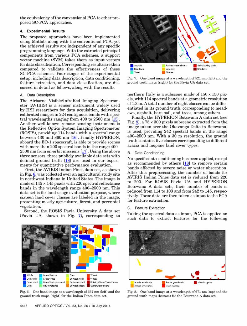
Finally, the HYPERION Botswana A data set (seeFig. 8), a 75 × 300 pixels subscene extracted from theimage taken over the Okavango Delta in Botswana,is used, providing 242 spectral bands in the range400–2500 nm. With a 30 m resolution, the groundtruth contains five classes corresponding to differentacacia and mopane land cover types.

B. Data Conditioning

No specific data conditioning has been applied, exceptas recommended by others [18] to remove certainbands affected by severe noise or water absorption.After this preprocessing, the number of bands forAVIRIS Indian Pines data set is reduced from 220to 200. For ROSIS Pavia UA and HYPERIONBotswana A data sets, their number of bands isreduced from 114 to 103 and from 242 to 145, respec-tively. These data are then taken as input to the PCAfor feature extraction.

C. Feature Extraction

Taking the spectral data as input, PCA is applied onsuch data to extract features for the following

Fig. 6. One band image at a wavelength of 667 nm (left) and theground truth maps (right) for the Indian Pines data set.

Fig. 7. One band image at a wavelength of 521 nm (left) and theground truth maps (right) for the Pavia UA data set.

Fig. 8. One band image at a wavelength of 671 nm (top) and theground truth maps (bottom) for the Botswana A data set.


classification tasks. Implemented in Matlab, the con-ventional PCA and the proposed SC-PCA strategiesare employed for feature extraction, respectively.Therefore, in total five approaches are compared,which include

– Conventional PCA (PCA)– Pixel-based SC-PCA (SC-PCA/P)– Row-based SC-PCA (SC-PCA/R)– Column-based SC-PCA (SC-PCA/C)– Band-based SC-PCA (SC-PCA/B).

D. Data Classification

The SVM classifier is implemented using LIBSVM[19], a publicly available library with interface toMatlab. Although the classifier supports several ker-nels including linear, polynomial, and Gaussian ra-dial basis function (RBF), it is found that theGaussian RBF kernel produces particular good re-sults. Consequently, the RBF kernel is selected in allour experiments, and this is consistent with findingsfrom many other researchers [20,21]. To learn theSVM model, the training ratio is always fixed at arelatively low value of 30%. The number of PCA re-duced components is tested on the interval 1–10.

The data sets are randomly split for training andtesting by stratified sampling inside each class in theground truth. This is repeated 10 times providing atotal of 10 possible experiments. Two parameters forthe RBF kernel, the penalty C and the gamma γ, areoptimized for every experiment in the training proc-ess through a grid search. For the five PCA ap-proaches, the mean classification rate in terms ofoverall accuracy and the standard deviation overthe 10 experiments are obtained for performanceevaluation. These are reported in the following.

E. Results and Discussion

First of all, classification rates using features fromthe different PCA approaches is compared in Table 2,where the numbers of principal components used forclassification is 10. As can be seen, the results fromthese five PCA approaches are exactly the same.

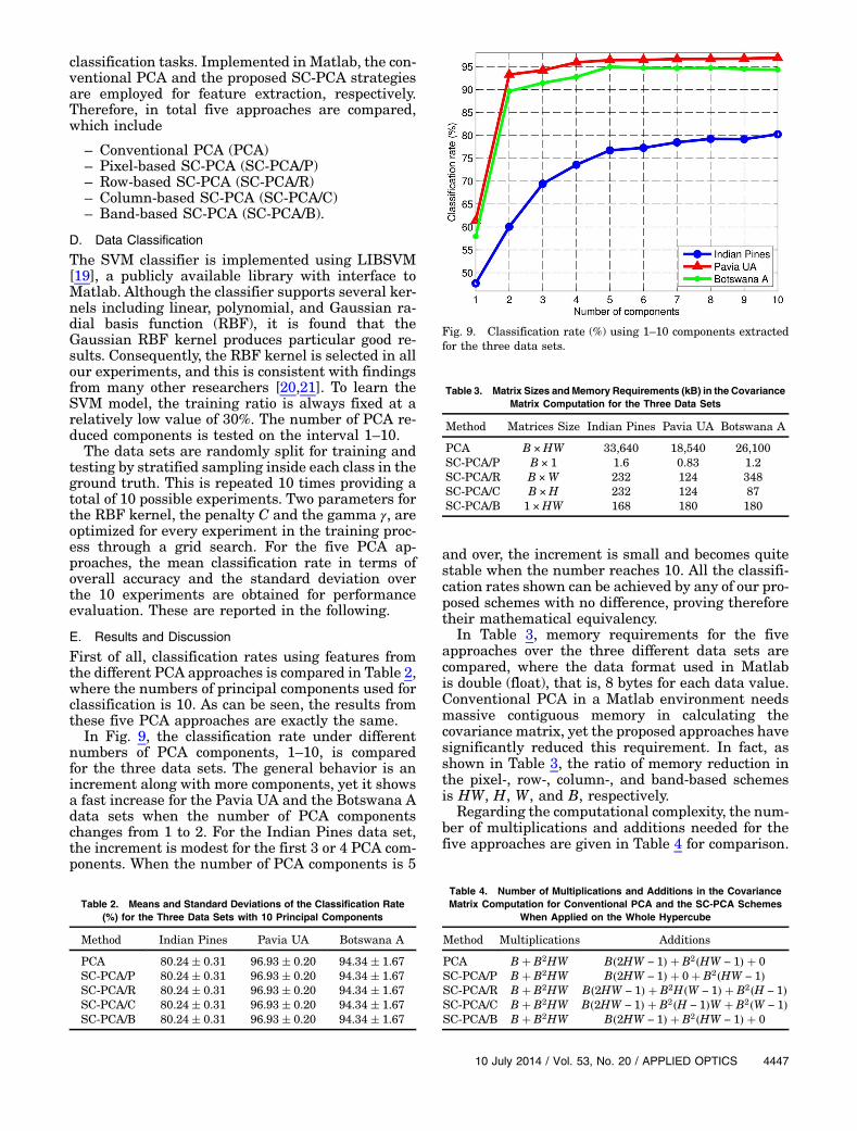
In Fig. 9, the classification rate under differentnumbers of PCA components, 1–10, is comparedfor the three data sets. The general behavior is anincrement along with more components, yet it showsa fast increase for the Pavia UA and the Botswana Adata sets when the number of PCA componentschanges from 1 to 2. For the Indian Pines data set,the increment is modest for the first 3 or 4 PCA com-ponents. When the number of PCA components is 5

and over, the increment is small and becomes quitestable when the number reaches 10. All the classifi-cation rates shown can be achieved by any of our pro-posed schemes with no difference, proving thereforetheir mathematical equivalency.

In Table 3, memory requirements for the fiveapproaches over the three different data sets arecompared, where the data format used in Matlabis double (float), that is, 8 bytes for each data value.Conventional PCA in a Matlab environment needsmassive contiguous memory in calculating thecovariance matrix, yet the proposed approaches havesignificantly reduced this requirement. In fact, asshown in Table 3, the ratio of memory reduction inthe pixel-, row-, column-, and band-based schemesis HW, H, W, and B, respectively.

Regarding the computational complexity, the num-ber of multiplications and additions needed for thefive approaches are given in Table 4 for comparison.

Table 2. Means and Standard Deviations of the Classification Rate

(%) for the Three Data Sets with 10 Principal Components

Method Indian Pines Pavia UA Botswana A

PCA 80.24� 0.31 96.93� 0.20 94.34� 1.67SC-PCA/P 80.24� 0.31 96.93� 0.20 94.34� 1.67SC-PCA/R 80.24� 0.31 96.93� 0.20 94.34� 1.67SC-PCA/C 80.24� 0.31 96.93� 0.20 94.34� 1.67SC-PCA/B 80.24� 0.31 96.93� 0.20 94.34� 1.67

Fig. 9. Classification rate (%) using 1–10 components extractedfor the three data sets.

Table 3. Matrix Sizes and Memory Requirements (kB) in the Covariance

Matrix Computation for the Three Data Sets

Method Matrices Size Indian Pines Pavia UA Botswana A

PCA B ×HW 33,640 18,540 26,100SC-PCA/P B × 1 1.6 0.83 1.2SC-PCA/R B ×W 232 124 348SC-PCA/C B ×H 232 124 87SC-PCA/B 1 ×HW 168 180 180

Table 4. Number of Multiplications and Additions in the Covariance

Matrix Computation for Conventional PCA and the SC-PCA Schemes

When Applied on the Whole Hypercube

Method Multiplications Additions

PCA B� B2HW B�2HW − 1� � B2�HW − 1� � 0

SC-PCA/P B� B2HW B�2HW − 1� � 0� B2�HW − 1�

SC-PCA/R B� B2HW B�2HW − 1� � B2H�W − 1� � B2�H − 1�

SC-PCA/C B� B2HW B�2HW − 1� � B2�H − 1�W � B2�W − 1�

SC-PCA/B B� B2HW B�2HW − 1� � B2�HW − 1� � 0


The multiplications contain two parts: the first is forthe mean-adjustment implementation, while the sec-ond is for the covariance matrix construction. On theother hand, the additions needed contain three parts:the first for the mean adjustment, the second forcalculating the partial covariance matrices, and thethird for their summation. Not surprisingly, thenumber of required multiplications and additionsis exactly the same, yet these operations are differ-ently distributed.

In the following, the numbers of multiplicationsand additions needed for real-time covariance com-putation in the four SC-PCA approaches are com-pared. In Table 5, the computational complexity ineach loop is shown. As can be seen, SC-PCA/P hasthe minimum required computations in each loop,yet it takes HW sequential scans to complete theacquisition process. In contrast, the other threeSC-PCA approaches have more computations in eachloop, yet the overall number of sequential scans ismuch reduced. The total computational cost in com-puting the covariance matrix for all the SC-PCAapproaches is almost the same.

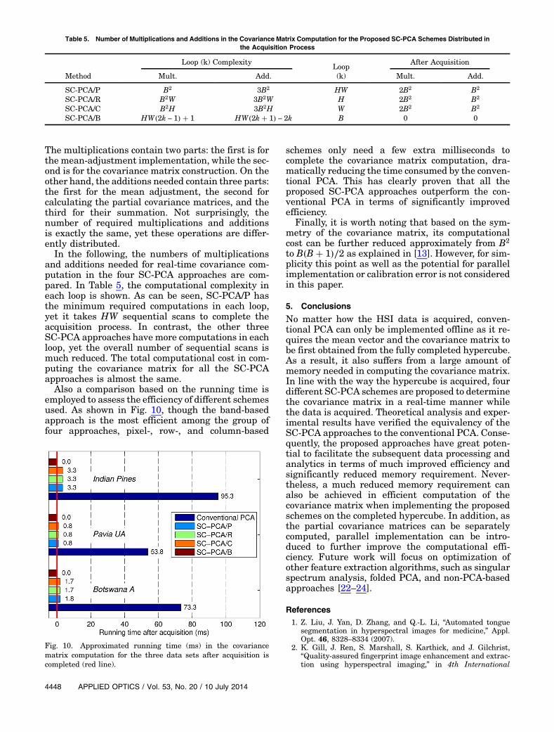
Also a comparison based on the running time isemployed to assess the efficiency of different schemesused. As shown in Fig. 10, though the band-basedapproach is the most efficient among the group offour approaches, pixel-, row-, and column-based

schemes only need a few extra milliseconds tocomplete the covariance matrix computation, dra-matically reducing the time consumed by the conven-tional PCA. This has clearly proven that all theproposed SC-PCA approaches outperform the con-ventional PCA in terms of significantly improvedefficiency.

Finally, it is worth noting that based on the sym-metry of the covariance matrix, its computationalcost can be further reduced approximately from B2

to B�B� 1�∕2 as explained in [13]. However, for sim-plicity this point as well as the potential for parallelimplementation or calibration error is not consideredin this paper.

5. Conclusions

No matter how the HSI data is acquired, conven-tional PCA can only be implemented offline as it re-quires the mean vector and the covariance matrix tobe first obtained from the fully completed hypercube.As a result, it also suffers from a large amount ofmemory needed in computing the covariance matrix.In line with the way the hypercube is acquired, fourdifferent SC-PCA schemes are proposed to determinethe covariance matrix in a real-time manner whilethe data is acquired. Theoretical analysis and exper-imental results have verified the equivalency of theSC-PCA approaches to the conventional PCA. Conse-quently, the proposed approaches have great poten-tial to facilitate the subsequent data processing andanalytics in terms of much improved efficiency andsignificantly reduced memory requirement. Never-theless, a much reduced memory requirement canalso be achieved in efficient computation of thecovariance matrix when implementing the proposedschemes on the completed hypercube. In addition, asthe partial covariance matrices can be separatelycomputed, parallel implementation can be intro-duced to further improve the computational effi-ciency. Future work will focus on optimization ofother feature extraction algorithms, such as singularspectrum analysis, folded PCA, and non-PCA-basedapproaches [22–24].

References

1. Z. Liu, J. Yan, D. Zhang, and Q.-L. Li, “Automated tonguesegmentation in hyperspectral images for medicine,” Appl.Opt. 46, 8328–8334 (2007).

2. K. Gill, J. Ren, S. Marshall, S. Karthick, and J. Gilchrist,“Quality-assured fingerprint image enhancement and extrac-tion using hyperspectral imaging,” in 4th International

Table 5. Number of Multiplications and Additions in the Covariance Matrix Computation for the Proposed SC-PCA Schemes Distributed in

the Acquisition Process

Method

Loop (k) ComplexityLoop(k)

After Acquisition

Mult. Add. Mult. Add.

SC-PCA/P B2 3B2 HW 2B2 B2

SC-PCA/R B2W 3B2W H 2B2 B2

SC-PCA/C B2H 3B2H W 2B2 B2

SC-PCA/B HW�2k − 1� � 1 HW�2k� 1� − 2k B 0 0

Fig. 10. Approximated running time (ms) in the covariancematrix computation for the three data sets after acquisition iscompleted (red line).


Conference on Imaging for Crime Detection and Prevention,London (2011).

3. S. Sumriddetchkajorn and Y. Intaravanne, “Hyperspectralimaging-based credit card verifier structure with adaptivelearning,” Appl. Opt. 47, 6594–6600 (2008).

4. T. Kelman, J. Ren, and S. Marshall, “Effective classification ofChinese tea samples in hyperspectral imaging,” Artific. Intell.Res. 2, 87–96 (2013).

5. C. Zhao, X. Li, J. Ren, and S. Marshall, “Improved sparse rep-resentation using adaptive spatial support for effective targetdetection in hyperspectral imagery,” Int. J. Remote Sens. 34,8669–8684 (2013).

6. S. E. Craig, S. E. Lohrenz, Z. Lee, K. L. Mahoney, G. J.Kirkpatrick, O. M. Schofield, and R. G. Steward, “Use ofhyperspectral remote sensing reflectance for detection and as-sessment of the harmful alga, Karenia brevis,” Appl. Opt. 45,5414–5425 (2006).

7. G. F. Hughes, “On the mean accuracy of statistical patternrecognition,” IEEE Trans. Inf. Theory 14, 55–63 (1968).

8. H. Abdi and L. J. Williams, Principal Component Analysis(WIREs Comp Stat, 2010).

9. R. Dianat and S. Kasaei, “Dimension reduction of optical re-mote sensing images via minimum change rate deviationmethod,” IEEE Trans. Geosci. Remote Sens. 48, 198–206(2010).

10. T. W. Du Bosq, J. M. Lopez-Alonso, and G. D. Boreman, “Milli-meter wave imaging system for land mine detection,” Appl.Opt. 45, 5686–5692 (2006).

11. F. Ndi, F. Adar, and S. H. Atzeni, “Spectral imaging,” Readout38, 68–73 (2011).

12. F. Vagni, “Survey of hyperspectral and multispectral imagingtechnologies,” NATO Tech. Rep., 2007.

13. R. Jošth, J. Antikainen, J. Havel, A. Herout, P. Zemčík, andM.Hauta-Kasari, “Real-time PCA calculation for spectral imag-ing (using SIMD and GP-GPU),” J. Real Time Image Proc. 7,1–9 (2012).

14. M.-Z. Wang, D.-M. Wang, W.-X. Xu, B.-Y. Chen, and K.Guo, “Parallel computing of covariance matrix and its appli-cation on hyperspectral data process,” in Geoscience andRemote Sensing Symposium (IGARSS), July 22–27, 2012,pp. 4058–4061.

15. R. O. Green, M. L. Eastwood, C. M. Sarture, T. G. Chrien, M.Aronsson, B. J. Chippendale, J. A. Faust, B. E. Pavri, C. J.Chovit, M. Solis, M. R. Olah, and O. Williams, “Imagingspectroscopy and the airborne visible/infrared imaging spec-trometer (AVIRIS),” Remote Sens. Environ. 65, 227–248(1998).

16. S. Holzwarth, A. Müller, M. Habermeyer, R. Richter, A.Hausold, S. Thiemann, and P. Strohl, “HySens-DAIS 7915/ROSIS imaging spectrometers at DLR,” in Proceedings ofthe 3rd Earsel Workshop on Imaging Spectroscopy, Herrsch-ing, Germany, May 13–16, 2003, pp. 3–14.

17. J. S. Pearlman, P. S. Barry, C. C. Segal, J. Shepanski, D. Beiso,and S. L. Carman, “Hyperion, a space-based imagingspectrometer,” IEEE Trans. Geosci. Remote Sens. 41,1160–1173, (2003).

18. “Hyperspectral remote sensing scenes,” 2014, http://www.ehu.es/ccwintco/index.php/Hyperspectral_Remote_Sensing_Scenes.

19. C. C. Chang and C. J. Lin, “LIBSVM: a library for supportvector machines,” ACM Trans. Intell. Syst. Technol. 2, 1–27(2013).

20. F. Melgani and L. Bruzzone, “Classification of hyperspectralremote sensing images with support vector machines,” IEEETrans. Geosci. Remote Sens. 42, 1778–1790 (2004).

21. M. Rojas, I. Dópido, A. Plaza, and P. Gamba, “Comparison ofsupport vector machine-based processing chains for hyper-spectral image classification,” Proc. SPIE 7810, 78100B(2010).

22. J. Zabalza, J. Ren, Z. Wang, S. Marshall, and J. Wang, “Singu-lar spectrum analysis for effective feature extraction inhyperspectral imaging,” IEEE Geosci. Remote Sens. Lett.11, 1886–1890 (2014).

23. J. Zabalza, J. Ren, M. Yang, Y. Zhang, J. Wang, S. Marshall,and J. Han, “Novel folded-PCA for improved feature extrac-tion and data reduction with hyperspectral imaging andSAR in remote sensing,” ISPRS J. Photogr. Remote Sens.93, 112–122 (2014).

24. J. Ren, J. Zabalza, S. Marshall, and J. Zheng, “Effective fea-ture extraction and data reduction with hyperspectral imag-ing in remote sensing,” IEEE Signal Process. Mag. 31(4),149–154 (2014).


http://www.ehu.es/ccwintco/index.php/Hyperspectral_Remote_Sensing_Scenes





zabalza, jaime and ren, jinchang and ren, jie and liu, zhe ... · jaime zabalza,1 jinchang ren,1,*...

Documents