X-ray fluorescence analysis for the study of fragments potteryexcavated at Tell Jendares site, Syria, employing multivariatestatistical analysis

E. H. Bakraji • M. Itlas • A. Abdulrahman •

H. Issa • R. Abboud

Received: 8 February 2010 / Published online: 14 May 2010

� Akademiai Kiado, Budapest, Hungary 2010

Abstract X-ray fluorescence analysis study of 44

archaeological pottery samples collected from Tell Jend-

ares site north-west of Syria has been carried out. Four

samples of the total previous investigated samples were

obtained from the kiln found on Tell Jendares site. Sev-

enteen different chemical elements were determined. The

XRF results have been processed using two multivariate

statistical cluster and factor analysis methods in order to

determine the similarities and correlation between the

selected samples based on their elemental composition.

The methodology successfully separates the samples where

three distinct chemical groups were discerned.

Keywords X-ray � Pottery � Archaeology �Multivariate analysis � Syria

Introduction

In view of the considerable Syrian heritage, special atten-

tion was given recently to physical instrumental analysis

science applications in archaeology, such as X-ray fluo-

rescence (XRF), particle induced X-ray emission (PIXE),

thermo luminescence (TL), etc. Archaeologists have been,

for many years, interested in the provenance of pottery

fragments, since pottery is the most abundant tracer in all

archaeological excavation. The analysis of pottery can

indeed supplement the information gathered from written

documents to produce a better knowledge of trade routes

linking populations of different areas, which is one of the

essential in gradients for the comprehension of their his-

tory. The microscopic properties of pottery such as

chemical composition may answer questions concerning

origin [1].

Chemical composition of pottery from major, minor and

trace elements provides a compositional ‘‘fingerprint’’ for

grouping together pottery made from the same raw mate-

rials and for distinguishing between groups of pottery made

from different raw material [2]. In the early days of

provenance studies using chemical analysis the principal

analytical techniques were instrumental neutron activation

analysis (INAA), and X-ray fluorescence (XRF). Since the

initial pottery study by Sayer and Dosden in 1957 [3],

many techniques have been widely exploited in the study

of archaeological pottery, such as INAA [4–6], XRF, PIXE

[7–13], and inductively coupled plasma emission analysis

[14]. The trace constituents-elements which are present in

amount below 1.000 ppm that provides the primary basis

for provenience analysis. XRF, a very sensitive non-

destructive method for analyzing the content of various

chemical elements in material, is an excellent tool for

investigations of historic relics, works of art and archaeo-

logical finds [15, 16]. The XRF method have been applied

in our laboratory to analyze different kind of samples,

among them archaeological pottery [12, 13]. XRF is low-

cost and rapid technique for the determining the major,

minor and trace element composition of pottery [17, 18],

XRF can analyze some 15–30 elements with atomic

E. H. Bakraji (&) � H. Issa � R. Abboud

Department of Chemistry, Atomic Energy Commission,

P.O. Box 6091, Damascus, Syria

e-mail: cscientific@aec.org.sy

M. Itlas

Department of Scientific Service, Atomic Energy Commission,

P.O. Box 6091, Damascus, Syria

A. Abdulrahman

Director of Tell Jendares Mission, Albassel Centre for

Archaeological Training, Atomic Energy Commission,

P.O. Box 6091, Damascus, Syria

123

J Radioanal Nucl Chem (2010) 285:455–460

DOI 10.1007/s10967-010-0595-4

numbers ranging from Z = 11 to Z = 41 and some of the

rare earth elements (REEs) [19, 20].

In this work, we applied the XRF technique to analyze

archaeological pottery recovered during the 2006 and 2007

field seasons of the Syrian–German Expedition to the Tell

Jendares site. Seventeen chemical elements were deter-

mined. These elemental concentrations have been pro-

cessed using statistical method in order to determine

similarity and correlation between the various samples. The

first aim of our study was to classify pottery into groups

having similar elemental composition, which are assumed

to correspond to the same provenance. The determination

of provenance of pottery is of special interest, as it gives

valuable insight into ancient trade connection. The second

aim was providing database on additional chemical com-

position of archaeological pottery in Syria. Provenance

studies based on chemical composition involve then the

analysis of a large number of samples. In selecting pottery

samples for analysis, it is important that the samples are

from a single period and site.

Description of area and materials

Tell Jendares is located north-west of Syria (36� 220 N, 40�360 E), at the heart of this Tell exist the Alomek plain,

which represent a key milestone in this geographically part

of Syria. Alomek plain extends from the north-east to the

south-west among the Mont Simon in the east and moun-

tains Alomanus in the West.

The plain starts from the north of the Syrian–Turkish

border and ends at the south-west coast of the Mediterra-

nean, where the mouth of the Orontes river. The archaeo-

logical hill (Tell Jendares) exists in the south-west of the

Jendares town. Tell Jendares has a semi circular form and

the average diameter of the reminder of this Tell is about

450 m. Tell Jendares is located in plain at an altitude of

200 meters above sea level. The highest level of the Tell

Jendares is 31 m above the surrounding plain. Tell Jend-

ares contains consecutive settlements dating back to the

second millennium BC, where it is expected to be the

capital of Alomek plain and its name was ‘‘Anek’’ at that

time. In the first millennium BC, the Assyrian text indicates

that the name of the city Jendares was ‘‘Konaloa’’ at that

time, and it was the capital of Alomek area as well. It was

also mentioned that it was a rich city, has handed donations

and gifts to the Assyrian king Ashur Nasir Pal II, to avoid

the conflict with him.

All subsequent settlements belong to the classical per-

iod, which constitute recolonization since the Hellenistic

period to the Byzantine period, and the hill was called

‘‘Jindaros’’.

The 44 samples analyzed are unglazed and not decorated

earthenware and fairly representative of Hellenistic-Roman

pottery made between 300 BC and 100 AD. Four samples

of the total samples derive from the kiln found on the site

(samples K41, K42, K43, and K44).

Experimental

Sample preparation

After removal of the surface deposit, pottery samples were

ground into a fine powder for 10–15 min, using an agate

motor. All samples powder were then dried at 105 �C for

24 h and stored in desiccators until they were measured,

where pellets from pressed powder were performed.

Instrumentation and measurements

The analyses of the thick pellets (25 mm diameter) from

pressed powder were performed using an EDXRF spec-

trometer assembled by the Syrian Atomic Energy Com-

mission. The unit is equipped with a Molybdenum X-ray

tube (Philips) with Mo secondary target, controller and

cooling system from (ItalStructures), Si(Li) detector and its

electronics (H.V. power supply, Amp., ADC and MCA)

from PGT, system 4000. The Si(Li) detector has an energy

resolution 140 eV at 5.9 keV for the Mn–Ka. The X-ray

tube was operated at 35 kV, 20 mA at 1000 s live time to

generate X-ray intensity ka, La lines data for the following

elements: bromine (Br) calcium (Ca), copper (Cu), chro-

mium (Cr), gallium (Ga), iron (Fe), lead (Pb) (from La),

manganese (Mn), nickel (Ni), potassium (K), rubidium

(Rb), strontium (Sr), titanium (Ti), and zinc (Zn). For the

elements niobium (Nb), yttrium (Y), and zirconium (Zr),

Ka line data were generated by using a cadmium (109Cd)

radioisotope source (*9 9 108 Bq) for 1000 s live time.

X-ray fluorescence outgoing from the samples were carried

out with qualitative and quantitative X-ray analysis pro-

gram (QXAS) from the International Atomic Energy

Agency (IAEA). The net peak intensities of the Ka and Lalines were calculated by fitting the spectra with the sub-

program AXIL (version 3.6) [21].

One of the implemented procedures in the QXAS

package is called elemental sensitivities in sub-program the

simple quantitative analysis (S.Q.A.), which is used to

determine the sensitivity of X-ray lines, taking into account

the X-ray attenuation in the standard used for calibration.

The standards used in our study to establish the sensitivity

curves are the following: Ti; Cr; Fe; Cu; Zn; Zr; as foils; S;

Ni; Se; as powder pure elements; KH2PO4; CaCO3; KCl;

KBr; As2O3 and SrCO3 as chemical compounds; for Ka

456 E. H. Bakraji et al.

123

lines; Pt; Pb and U as foils; CsCl3; La2O3; Nd2O3; Gd2O3;

WO3 as chemical compounds; for La lines.

Soil-7 (IAEA); sediments SL-1 and SL-3 (IAEA) were

used as standards samples for testing the accuracy of sen-

sitivity curves. The S.Q.A. is then used to determine the

concentrations of the elements in the unknown samples

with the possibility to take X-ray attenuation into account.

More details about the S.Q.A. method are described in

[21]. All of the XRF data analyses were the results of

averaging three measurements for each pottery sample. The

repeated analyses of several samples showed that in each

case the relative standard deviation (RSD) was less than

5% for each element under investigation.

Statistical treatment

The Statistical 6.0 package was used in this work for all

statistical calculations. The final data which consists of

observations (samples) and variables (elements) have been

processed using two multivariate statistical methods,

cluster analysis (CA), and factor analysis (FA). Cluster

analysis is often used in the initial inspection of data

because it is a rapid and efficient technique for evaluating

relationships between a large numbers of samples, between

which distance measures have been calculated [22]. CA

classifies samples into distinct groups and the results are

commonly presented as dendrogram showing the order and

levels of clustering as well as the distances between indi-

vidual samples.

A primary goal of factor analysis is to extract a mini-

mum number of factors which explains an acceptable

amount of total variance of the data set. In order to explain

100% of the variance in the data set, the number of factors

retained should necessarily be equal to the number of

elements chosen for statistical analysis. In general we

choose a number of factors that explain at least 70% of the

total variance, and generally the three-first factors are

sufficient to reach this value. For the present work the

three-first factors were adequate to explain, as we will see

later, more than 70% of the total variance. The method for

factor extraction used in this study was principal compo-

nents; the method utilized for rotation was varimax.

Results and discussion

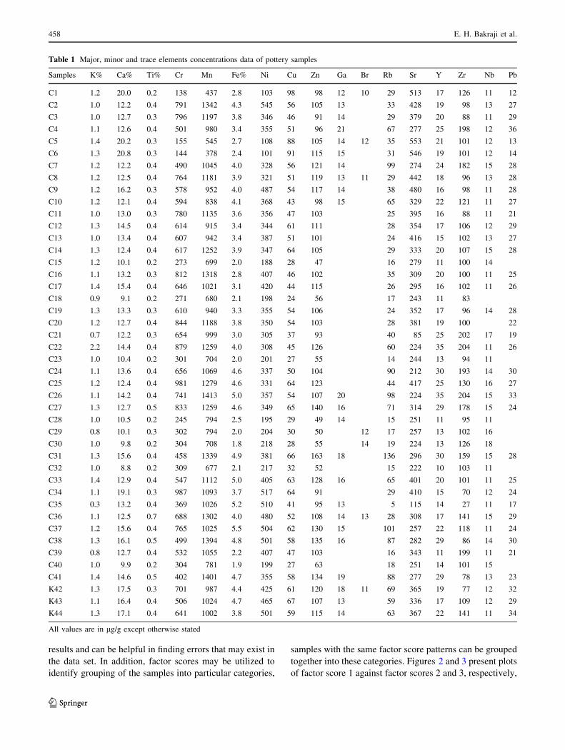
Table 1 lists the concentration of major, minor, and trace

elements found in the pottery analyzed. It is clear from this

table that there are large variations in the elemental con-

centrations among the samples. All the elements in the data

set with precision better than 10% were considered because

if an element is not measured with good precision it

can obscure real differences in concentration, and the

discriminating effect of other well-measured element tends

to be reduced. In the present work the precision was better

than 10% for all determined elements. In the other hand all

elements that have more than 25% missing values across

the samples set were not introduced in the data set for

multivariate analysis, this is the case of the elements gal-

lium (Ga) and bromine (Br). The procedure used to esti-

mate the missing values for other element in the data set

was to replace any missing value by the minimum detec-

tion limits (MDL) determined by XRF, this is the case of

the two elements niobium (Nb) and lead (Pb) were the

MDL is 10 ppm for these elements.

Based on the screening criteria, only 15 elements were

used in the subsequent data analysis. The final data set

consisted of 44 samples (observations) with 15 elements

(variables) for a total of 660 data entries. The cluster and

factor analysis were performed from the base log.10

transformed concentration values, to normalize element

distribution and reduce the impact of differences in mag-

nitude for some of the major elements.

Cluster analysis (CA)

The resulting dendrogram is shown in Fig. 1. It was found

using single linkage as grouping rule, according to

Euclidean distance. It is clear that there are two main

clusters. Cluster 1 contains 31 samples (70% of the

observations), cluster 2 contains eight samples, and there is

one small cluster, cluster 3 which contains only three

samples (C1, C5, and C6).

Factor analysis (FA)

Table 2 shows the factor loading for the three extracted

factors. As listed on Table 2, factor 1 explains 28.6% of the

total variance of the data set, factor 2 explains 27.5% and

finally factor 3 explains 14.8%. It is clear that the three

factors extracted in this study explain 70.9.% of the total

variance of the data set. The square of the factor loading of

an element for a given factor indicates the fraction of

variance of the element which can be explained by the

common variance of that factor. For example the loading of

manganese (Mn) in Table 2 on factor 1 for the data set is

0.92, thus (0.92)2 = 85% of the variance of Mn can be

explained by the common variance of factor 1. The squared

factor loading of a particular element summed over all

factors is the communality of that element. It is clear from

Table 2 that the communalities for 80% of the elements are

greater than 50%. Therefore, the FA fit to the data set is

good. In addition to factor loading, this analysis yields

factor scores, which quantify the relative intensities of

factor strength on each sample. Factor scores are very

helpful in interpreting and understanding factor analysis

X-ray fluorescence 457

123

results and can be helpful in finding errors that may exist in

the data set. In addition, factor scores may be utilized to

identify grouping of the samples into particular categories,

samples with the same factor score patterns can be grouped

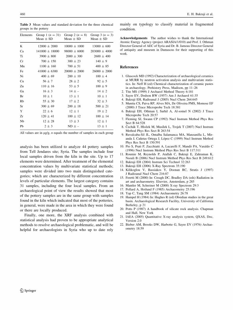
together into these categories. Figures 2 and 3 present plots

of factor score 1 against factor scores 2 and 3, respectively,

Table 1 Major, minor and trace elements concentrations data of pottery samples

Samples K% Ca% Ti% Cr Mn Fe% Ni Cu Zn Ga Br Rb Sr Y Zr Nb Pb

C1 1.2 20.0 0.2 138 437 2.8 103 98 98 12 10 29 513 17 126 11 12

C2 1.0 12.2 0.4 791 1342 4.3 545 56 105 13 33 428 19 98 13 27

C3 1.0 12.7 0.3 796 1197 3.8 346 46 91 14 29 379 20 88 11 29

C4 1.1 12.6 0.4 501 980 3.4 355 51 96 21 67 277 25 198 12 36

C5 1.4 20.2 0.3 155 545 2.7 108 88 105 14 12 35 553 21 101 12 13

C6 1.3 20.8 0.3 144 378 2.4 101 91 115 15 31 546 19 101 12 14

C7 1.2 12.2 0.4 490 1045 4.0 328 56 121 14 99 274 24 182 15 28

C8 1.2 12.5 0.4 764 1181 3.9 321 51 119 13 11 29 442 18 96 13 28

C9 1.2 16.2 0.3 578 952 4.0 487 54 117 14 38 480 16 98 11 28

C10 1.2 12.1 0.4 594 838 4.1 368 43 98 15 65 329 22 121 11 27

C11 1.0 13.0 0.3 780 1135 3.6 356 47 103 25 395 16 88 11 21

C12 1.3 14.5 0.4 614 915 3.4 344 61 111 28 354 17 106 12 29

C13 1.0 13.4 0.4 607 942 3.4 387 51 101 24 416 15 102 13 27

C14 1.3 12.4 0.4 617 1252 3.9 347 64 105 29 333 20 107 15 28

C15 1.2 10.1 0.2 273 699 2.0 188 28 47 16 279 11 100 14

C16 1.1 13.2 0.3 812 1318 2.8 407 46 102 35 309 20 100 11 25

C17 1.4 15.4 0.4 646 1021 3.1 420 44 115 26 295 16 102 11 26

C18 0.9 9.1 0.2 271 680 2.1 198 24 56 17 243 11 83

C19 1.3 13.3 0.3 610 940 3.3 355 54 106 24 352 17 96 14 28

C20 1.2 12.7 0.4 844 1188 3.8 350 54 103 28 381 19 100 22

C21 0.7 12.2 0.3 654 999 3.0 305 37 93 40 85 25 202 17 19

C22 2.2 14.4 0.4 879 1259 4.0 308 45 126 60 224 35 204 11 26

C23 1.0 10.4 0.2 301 704 2.0 201 27 55 14 244 13 94 11

C24 1.1 13.6 0.4 656 1069 4.6 337 50 104 90 212 30 193 14 30

C25 1.2 12.4 0.4 981 1279 4.6 331 64 123 44 417 25 130 16 27

C26 1.1 14.2 0.4 741 1413 5.0 357 54 107 20 98 224 35 204 15 33

C27 1.3 12.7 0.5 833 1259 4.6 349 65 140 16 71 314 29 178 15 24

C28 1.0 10.5 0.2 245 794 2.5 195 29 49 14 15 251 11 95 11

C29 0.8 10.1 0.3 302 794 2.0 204 30 50 12 17 257 13 102 16

C30 1.0 9.8 0.2 304 708 1.8 218 28 55 14 19 224 13 126 18

C31 1.3 15.6 0.4 458 1339 4.9 381 66 163 18 136 296 30 159 15 28

C32 1.0 8.8 0.2 309 677 2.1 217 32 52 15 222 10 103 11

C33 1.4 12.9 0.4 547 1112 5.0 405 63 128 16 65 401 20 101 11 25

C34 1.1 19.1 0.3 987 1093 3.7 517 64 91 29 410 15 70 12 24

C35 0.3 13.2 0.4 369 1026 5.2 510 41 95 13 5 115 14 27 11 17

C36 1.1 12.5 0.7 688 1302 4.0 480 52 108 14 13 28 308 17 141 15 29

C37 1.2 15.6 0.4 765 1025 5.5 504 62 130 15 101 257 22 118 11 24

C38 1.3 16.1 0.5 499 1394 4.8 501 58 135 16 87 282 29 86 14 30

C39 0.8 12.7 0.4 532 1055 2.2 407 47 103 16 343 11 199 11 21

C40 1.0 9.9 0.2 304 781 1.9 199 27 63 18 251 14 101 15

C41 1.4 14.6 0.5 402 1401 4.7 355 58 134 19 88 277 29 78 13 23

K42 1.3 17.5 0.3 701 987 4.4 425 61 120 18 11 69 365 19 77 12 32

K43 1.1 16.4 0.4 506 1024 4.7 465 67 107 13 59 336 17 109 12 29

K44 1.3 17.1 0.4 641 1002 3.8 501 59 115 14 63 367 22 141 11 34

All values are in lg/g except otherwise stated

458 E. H. Bakraji et al.

123

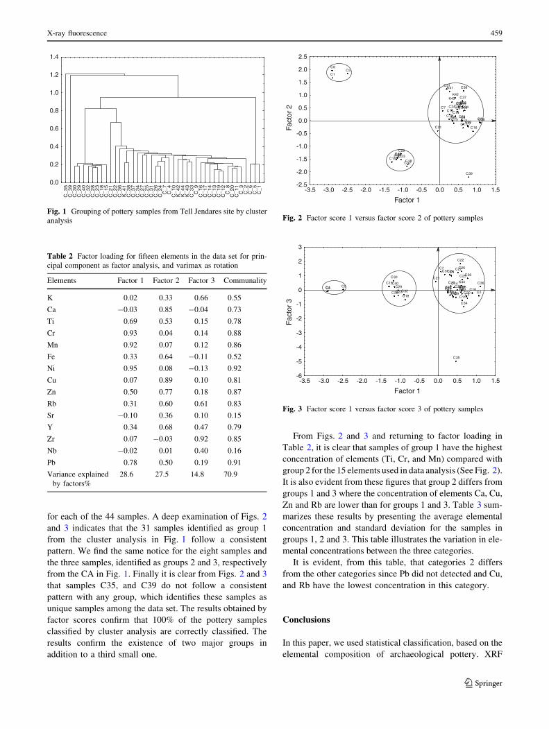
for each of the 44 samples. A deep examination of Figs. 2

and 3 indicates that the 31 samples identified as group 1

from the cluster analysis in Fig. 1 follow a consistent

pattern. We find the same notice for the eight samples and

the three samples, identified as groups 2 and 3, respectively

from the CA in Fig. 1. Finally it is clear from Figs. 2 and 3

that samples C35, and C39 do not follow a consistent

pattern with any group, which identifies these samples as

unique samples among the data set. The results obtained by

factor scores confirm that 100% of the pottery samples

classified by cluster analysis are correctly classified. The

results confirm the existence of two major groups in

addition to a third small one.

From Figs. 2 and 3 and returning to factor loading in

Table 2, it is clear that samples of group 1 have the highest

concentration of elements (Ti, Cr, and Mn) compared with

group 2 for the 15 elements used in data analysis (See Fig. 2).

It is also evident from these figures that group 2 differs from

groups 1 and 3 where the concentration of elements Ca, Cu,

Zn and Rb are lower than for groups 1 and 3. Table 3 sum-

marizes these results by presenting the average elemental

concentration and standard deviation for the samples in

groups 1, 2 and 3. This table illustrates the variation in ele-

mental concentrations between the three categories.

It is evident, from this table, that categories 2 differs

from the other categories since Pb did not detected and Cu,

and Rb have the lowest concentration in this category.

Conclusions

In this paper, we used statistical classification, based on the

elemental composition of archaeological pottery. XRF

Table 2 Factor loading for fifteen elements in the data set for prin-

cipal component as factor analysis, and varimax as rotation

Elements Factor 1 Factor 2 Factor 3 Communality

K 0.02 0.33 0.66 0.55

Ca -0.03 0.85 -0.04 0.73

Ti 0.69 0.53 0.15 0.78

Cr 0.93 0.04 0.14 0.88

Mn 0.92 0.07 0.12 0.86

Fe 0.33 0.64 -0.11 0.52

Ni 0.95 0.08 -0.13 0.92

Cu 0.07 0.89 0.10 0.81

Zn 0.50 0.77 0.18 0.87

Rb 0.31 0.60 0.61 0.83

Sr -0.10 0.36 0.10 0.15

Y 0.34 0.68 0.47 0.79

Zr 0.07 -0.03 0.92 0.85

Nb -0.02 0.01 0.40 0.16

Pb 0.78 0.50 0.19 0.91

Variance explained

by factors%

28.6 27.5 14.8 70.9

C_

35

C_

39

C_

30

C_

29

C_

40

C_

32

C_

28

C_

23

C_

18

C_

15

C_

21

C_

22

C_

36

K_

41

C_

38

C_

37

C_

34

C_

27

C_

25

C_

31

C_

26

C_

24

C_

7C

_4

C_

10

K_

42

K_

44

K_

43

C_

33

C_

9C

_1

6C

_1

7C

_1

4C

_1

3C

_1

9C

_1

2C

_8

C_

20

C_

11

C_

3C

_2

C_

6C

_5

C_

1

0.0

0.2

0.4

0.6

0.8

1.0

1.2

1.4

Fig. 1 Grouping of pottery samples from Tell Jendares site by cluster

analysis

C1

C2C3

C4

C5 C6

C7

C8

C9

C10

C11

C12

C13

C14

C15

C16

C17

C18

C19

C20

C21

C22

C23

C24 C25 C26 C27

C28 C29

C30

C31

C32

C33 C34 C35

C36

C37

C38

C39

C40

K41

K42 K43

K44

-3.5 -3.0 -2.5 -2.0 -1.5 -1.0 -0.5 0.0 0.5 1.0 1.5

Factor 1

-2.5

-2.0

-1.5

-1.0

-0.5

0.0

0.5

1.0

1.5

2.0

2.5

Fact

or 2

Fig. 2 Factor score 1 versus factor score 2 of pottery samples

C1C2

C3

C4

C5 C6

C7

C8 C9

C10

C11

C12 C13

C14 C15

C16 C17

C18

C19 C20

C21

C22

C23

C24 C25

C26 C27

C28

C29

C30

C31

C32 C33

C34

C35

C36 C37 C38

C39

C40 K41

K42 K43

K44

-3.5 -3.0 -2.5 -2.0 -1.5 -1.0 -0.5 0.0 0.5 1.0 1.5

Factor 1

-6

-5

-4

-3

-2

-1

0

1

2

3

Fac

tor

3

Fig. 3 Factor score 1 versus factor score 3 of pottery samples

X-ray fluorescence 459

123

analysis has been utilized to analyze 44 pottery samples

from Tell Jendares site; Syria. The samples include four

local samples driven from the kiln in the site. Up to 17

elements were determined. After treatment of the elemental

concentration values by multivariate statistical methods;

samples were divided into two main distinguished cate-

gories; which are characterized by different concentration

levels of particular elements. The largest category contains

31 samples, including the four local samples. From an

archaeological point of view the results showed that most

of the pottery samples are in the same group with samples

found in the kiln which indicated that most of the potteries,

in general, were made in the area in which they were found

or there are locally produced.

Finally, one more, the XRF analysis combined with

statistical analysis had proven to be appropriate analytical

methods to resolve archaeological problematic, and will be

helpful for archaeologists in Syria who up to date rely

mainly on typology to classify material in fragmented

condition.

Acknowledgements The author wishes to thank the International

Atomic Energy Agency (project ARASIA/1/010) and Prof. I. Othman

Director General of AEC of Syria and Dr. B. Jamous Director General

of antiquity and museum in Damascus for their supporting of this

work.

References

1. Glascock MD (1992) Characterization of archaeological ceramics

at MURR by neutron activation analysis and multivariate statis-

tics. In: Neff H (ed) Chemical characterization of ceramic pastes

in archaeology. Prehistory Press, Madison, pp 11–26

2. Tite MS (1999) J Archaeol Method Theory 6:181

3. Sayre EV, Dodson RW (1957) Am J Archaeol 61:35

4. Bakraji EH, Radioanal J (2005) Nucl Chem 264:645

5. Munita CS, Paiva RP, Alves MA, De Oliveira PMS, Momose EF

(2000) J Trace Microprobe Tech 18:381

6. Bakraji EH, Othman I, Sarhil A, Al-somel N (2002) J Trace

Microprobe Tech 20:57

7. Fleming SJ, Swann CP (1992) Nucl Instrum Method Phys Res

Sect B 64:528

8. Cechak T, Hlozek M, Musılek L, Trojek T (2007) Nucl Instrum

Method Phys Res Sect B 263:54

9. Ruvalcaba-Sil JL, Ontalba Salamanca MA, Manzanilla L, Mir-

anda J, Canetas Ortega J, Lopez C (1999) Nucl Instrum Method

Phys Res Sect B 150:591

10. Pio S, Prati P, Zucchiatti A, Lucarelli F, Mando PA, Varaldo C

(1996) Nucl Instrum Method Phys Res Sect B 117:311

11. Roumie M, Reynolds P, Atallah C, Bakraji E, Zahraman K,

Nsouli B (2006) Nucl Instrum Method Phys Res Sect B 249:612

12. Bakraji EH (2004) Instrum Sci Technol 32:263

13. Bakraji EH (2006) X-Ray Spectrom 35:190

14. Kilikoglou V, Bassiakos Y, Doonan RC, Stratis J (1997)

J Radioanal Nucl Chem 216:87

15. Feretti M (2000) In: Creagh DC, Bradley DA (eds) Radiation in

art and archaeometry. Elsevier, Amsterdam, p 285

16. Mantler M, Schreiner M (2000) X-ray Spectrom 29:3

17. Pollard A, Hoilund F (1985) Archaeometry 25:196

18. Yap C, Tang SM (1984) Archaeometry 26:78

19. Hampel H (1984) In: Hughes R (ed) Obsidian studies in the great

basin. Archaeological Research Facility, University of California

Berkeley, p 21

20. Potts P (1987) A handbook of silicate rock analysis. Chapman

and Hall, New York

21. IAEA (2005) Quantitative X-ray analysis system, QXAS, Doc,

Version 2.0

22. Bieber AM, Brooks DW, Harbotte G, Sayre EV (1976) Archae-

ometry 18:59

Table 3 Mean values and standard deviation for the three chemical

groups in the pottery

Elements Group 1 (n = 31) Group 2 (n = 8) Group 3 (n = 3)

Mean ± SD Mean ± SD Mean ± SD

K 12000 ± 2000 10000 ± 1000 13000 ± 600

Ca 141000 ± 18000 98000 ± 6000 203000 ± 4000

Ti 3900 ± 800 2000 ± 300 2600 ± 400

Cr 700 ± 150 300 ± 23 140 ± 9

Mn 1100 ± 160 700 ± 51 400 ± 85

Fe 41000 ± 6300 20000 ± 2000 26000 ± 2000

Ni 400 ± 69 200 ± 10 100 ± 4

Cu 56 ± 7 28 ± 2 92 ± 5

Zn 110 ± 16 53 ± 5 100 ± 9

Ga 16 ± 3 14 ± – 14 ± 2

Br 10 ± 1 13 ± 1 10 ± 1

Rb 55 ± 30 17 ± 2 32 ± 3

Sr 300 ± 69 200 ± 18 500 ± 21

Y 22 ± 6 12 ± 1 19 ± 2

Zr 120 ± 41 100 ± 12 100 ± 14

Nb 12 ± 28 13 ± 3 12 ± 1

Pb 2 ± 3 ND ± – 13 ± 1

All values are in lg/g, n equals the number of samples in each group

460 E. H. Bakraji et al.

123