www.bioalgorithms.infoan introduction to bioinformatics algorithms dynamic programming: edit...
Post on 19-Dec-2015
228 views
TRANSCRIPT
www.bioalgorithms.infoAn Introduction to Bioinformatics Algorithms
Dynamic Programming:Edit Distance
An Introduction to Bioinformatics Algorithms www.bioalgorithms.info
Outline
• DNA Sequence Comparison: First Success Stories• Change Problem• Manhattan Tourist Problem• Longest Paths in Graphs • Sequence Alignment• Edit Distance• Longest Common Subsequence Problem• Dot Matrices
An Introduction to Bioinformatics Algorithms www.bioalgorithms.info
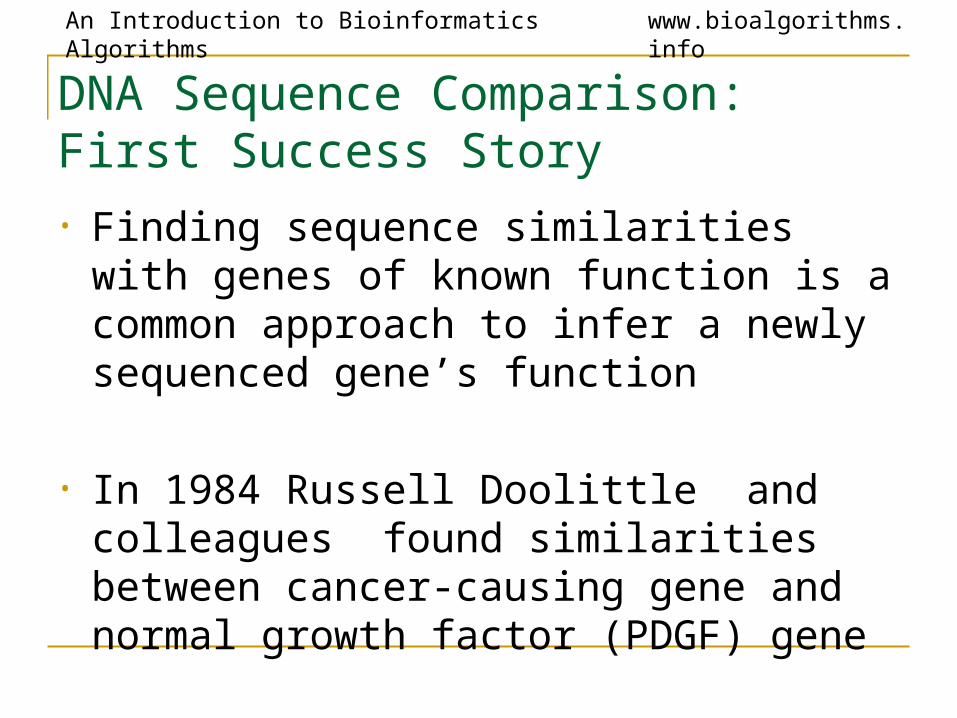
DNA Sequence Comparison: First Success Story • Finding sequence similarities with genes
of known function is a common approach to infer a newly sequenced gene’s function
• In 1984 Russell Doolittle and colleagues found similarities between cancer-causing gene and normal growth factor (PDGF) gene
An Introduction to Bioinformatics Algorithms www.bioalgorithms.info
Cystic Fibrosis
• Cystic fibrosis (CF) is a chronic and frequently fatal genetic disease of the body's mucus glands (abnormally high level of mucus in glands). CF primarily affects the respiratory systems in children.
• Mucus is a slimy material that coats many epithelial surfaces and is secreted into fluids such as saliva
An Introduction to Bioinformatics Algorithms www.bioalgorithms.info
Cystic Fibrosis: Inheritance
• In early 1980s biologists hypothesized that CF is an autosomal recessive disorder caused by mutations in a gene that remained unknown till 1989
• Heterozygous carriers are asymptomatic
• Must be homozygously recessive in this gene in order to be diagnosed with CF
An Introduction to Bioinformatics Algorithms www.bioalgorithms.info
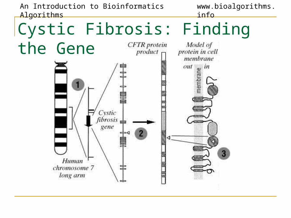
Cystic Fibrosis: Finding the Gene
An Introduction to Bioinformatics Algorithms www.bioalgorithms.info
Finding Similarities between the Cystic
Fibrosis Gene and ATP binding proteins
• ATP binding proteins are present on cell membrane and act as transport channel
• In 1989 biologists found similarity between the cystic fibrosis gene and ATP binding proteins
• A plausible function for cystic fibrosis gene, given the fact that CF involves sweet secretion with abnormally high sodium level
An Introduction to Bioinformatics Algorithms www.bioalgorithms.info
Cystic Fibrosis: Mutation Analysis
If a high % of cystic fibrosis (CF) patients have a certain mutation in the gene and the normal patients don’t, then that could be an indicator of a mutation that is related to CF
A certain mutation was found in 70% of CF patients, convincing evidence that it is a predominant genetic diagnostics marker for CF
An Introduction to Bioinformatics Algorithms www.bioalgorithms.info
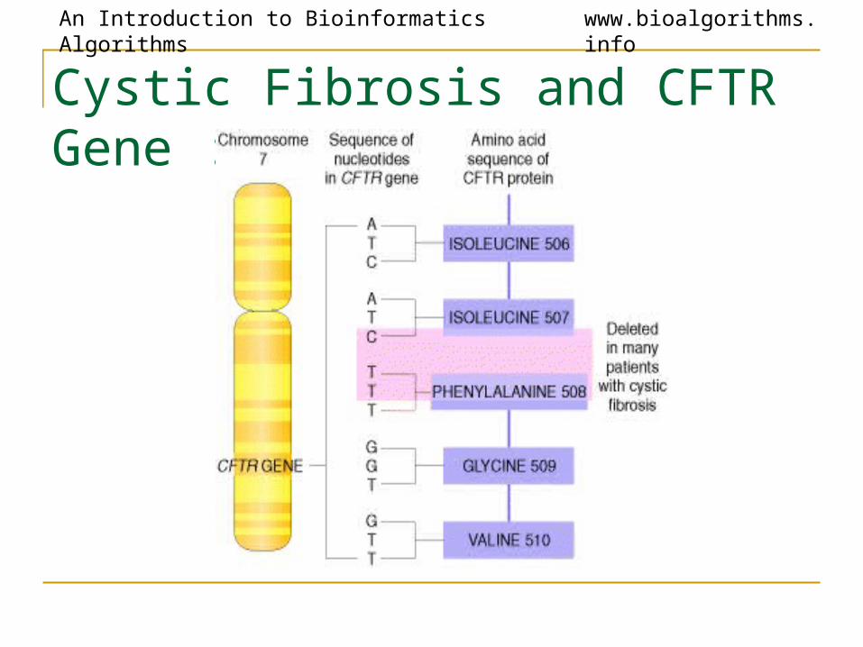
Cystic Fibrosis and CFTR Gene :
An Introduction to Bioinformatics Algorithms www.bioalgorithms.info
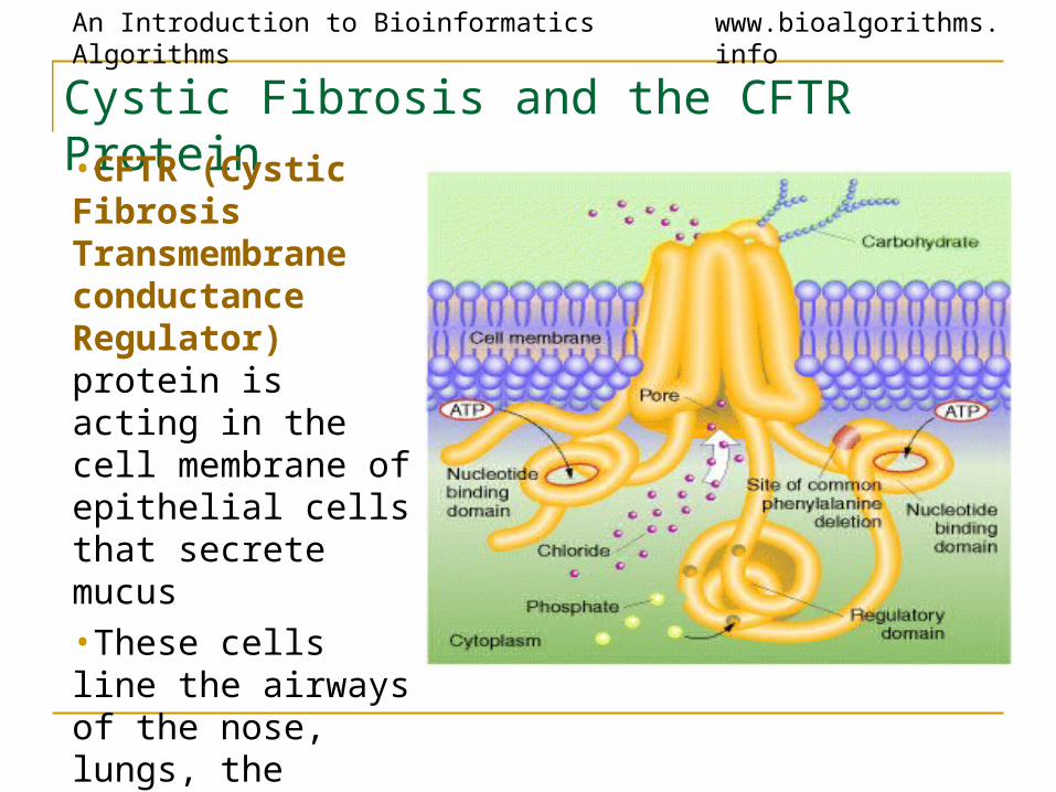
Cystic Fibrosis and the CFTR Protein•CFTR (Cystic Fibrosis Transmembrane conductance Regulator) protein is acting in the cell membrane of epithelial cells that secrete mucus•These cells line the airways of the nose, lungs, the stomach wall, etc.
An Introduction to Bioinformatics Algorithms www.bioalgorithms.info
Mechanism of Cystic Fibrosis
• The CFTR protein (1480 amino acids) regulates a chloride ion channel
• Adjusts the “wateriness” of fluids secreted by the cell
• Those with cystic fibrosis are missing one single amino acid in their CFTR
• Mucus ends up being too thick, affecting many organs
An Introduction to Bioinformatics Algorithms www.bioalgorithms.info
Bring in the Bioinformaticians• Gene similarities between two genes with
known and unknown function alert biologists to some possibilities
• Computing a similarity score between two genes tells how likely it is that they have similar functions
• Dynamic programming is a technique for revealing similarities between genes
• The Change Problem is a good problem to introduce the idea of dynamic programming
An Introduction to Bioinformatics Algorithms www.bioalgorithms.info
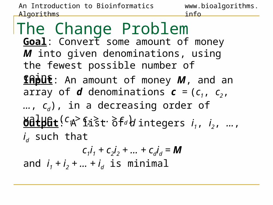
The Change ProblemGoal: Convert some amount of money M into given denominations, using the fewest possible number of coins
Input: An amount of money M, and an array of d denominations c = (c1, c2, …, cd), in a decreasing order of value (c1 > c2 > … > cd)
Output: A list of d integers i1, i2, …, id such that c1i1 + c2i2 + … + cdid = M
and i1 + i2 + … + id is minimal
An Introduction to Bioinformatics Algorithms www.bioalgorithms.info
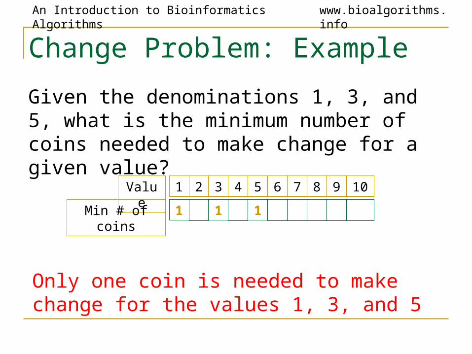
Change Problem: Example
Given the denominations 1, 3, and 5, what is the minimum number of coins needed to make change for a given value?
1 2 3 4 5 6 7 8 9 10
1 1 1
Value
Min # of coins
Only one coin is needed to make change for the values 1, 3, and 5
An Introduction to Bioinformatics Algorithms www.bioalgorithms.info
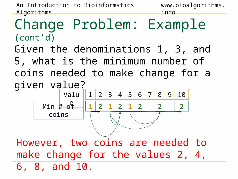
Change Problem: Example (cont’d)Given the denominations 1, 3, and 5, what is the minimum number of coins needed to make change for a given value?
1 2 3 4 5 6 7 8 9 10
1 2 1 2 1 2 2 2
Value
Min # of coins
However, two coins are needed to make change for the values 2, 4, 6, 8, and 10.
An Introduction to Bioinformatics Algorithms www.bioalgorithms.info
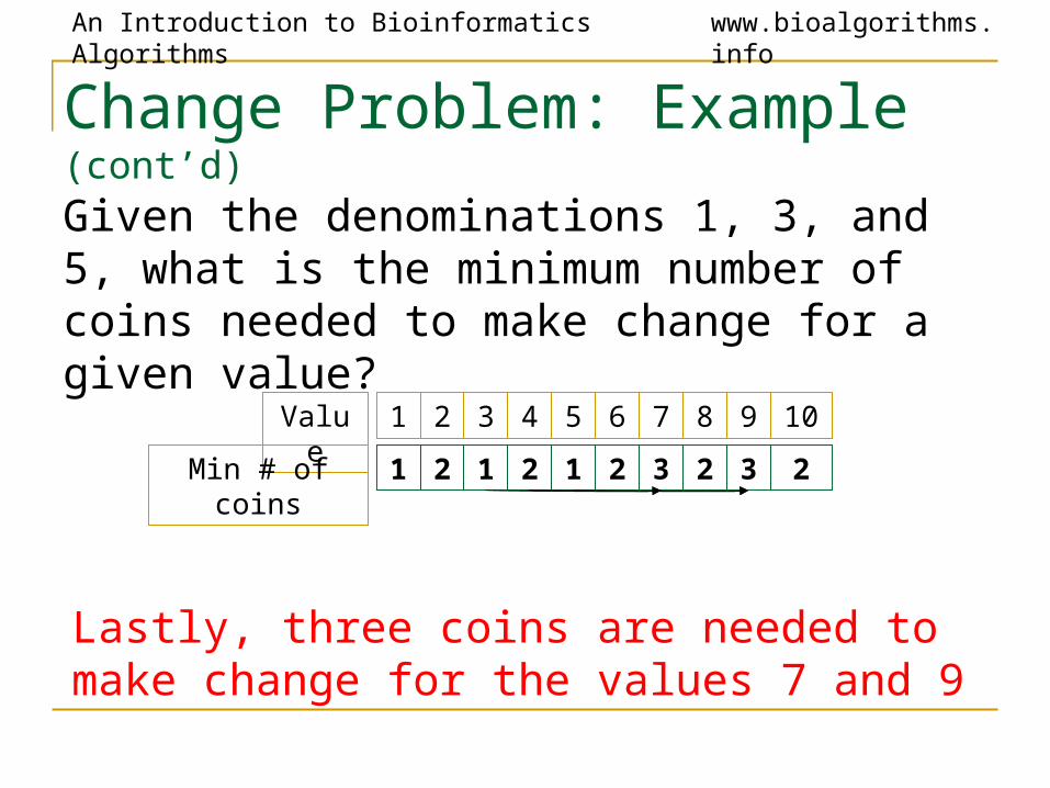
Change Problem: Example (cont’d)
1 2 3 4 5 6 7 8 9 10
1 2 1 2 1 2 3 2 3 2
Value
Min # of coins
Lastly, three coins are needed to make change for the values 7 and 9
Given the denominations 1, 3, and 5, what is the minimum number of coins needed to make change for a given value?
An Introduction to Bioinformatics Algorithms www.bioalgorithms.info
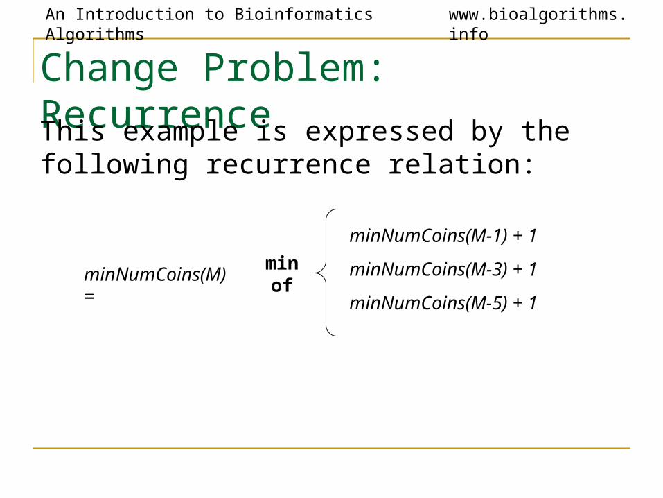
Change Problem: Recurrence
This example is expressed by the following recurrence relation:
minNumCoins(M) =
minNumCoins(M-1) + 1
minNumCoins(M-3) + 1
minNumCoins(M-5) + 1
min of
An Introduction to Bioinformatics Algorithms www.bioalgorithms.info
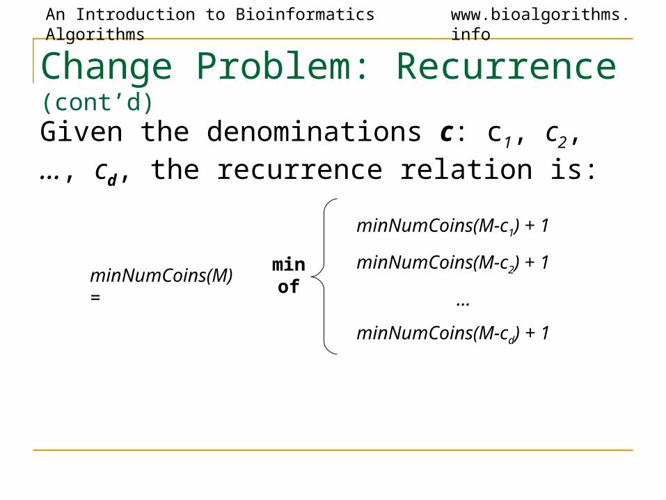
Change Problem: Recurrence (cont’d)Given the denominations c: c1, c2, …, cd, the recurrence relation is:
minNumCoins(M) =
minNumCoins(M-c1) + 1
minNumCoins(M-c2) + 1
…
minNumCoins(M-cd) + 1
min of
An Introduction to Bioinformatics Algorithms www.bioalgorithms.info
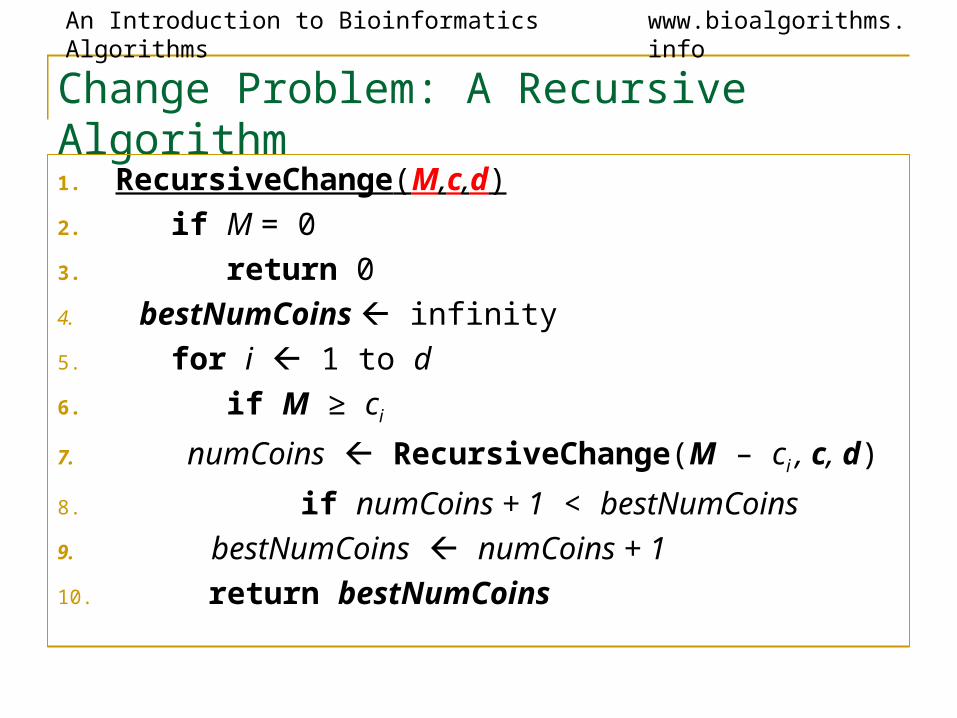
Change Problem: A Recursive Algorithm1. RecursiveChange(M,c,d)2. if M = 03. return 04. bestNumCoins infinity5. for i 1 to d6. if M ≥ ci
7. numCoins RecursiveChange(M – ci , c, d)
8. if numCoins + 1 < bestNumCoins9. bestNumCoins numCoins + 110. return bestNumCoins
An Introduction to Bioinformatics Algorithms www.bioalgorithms.info
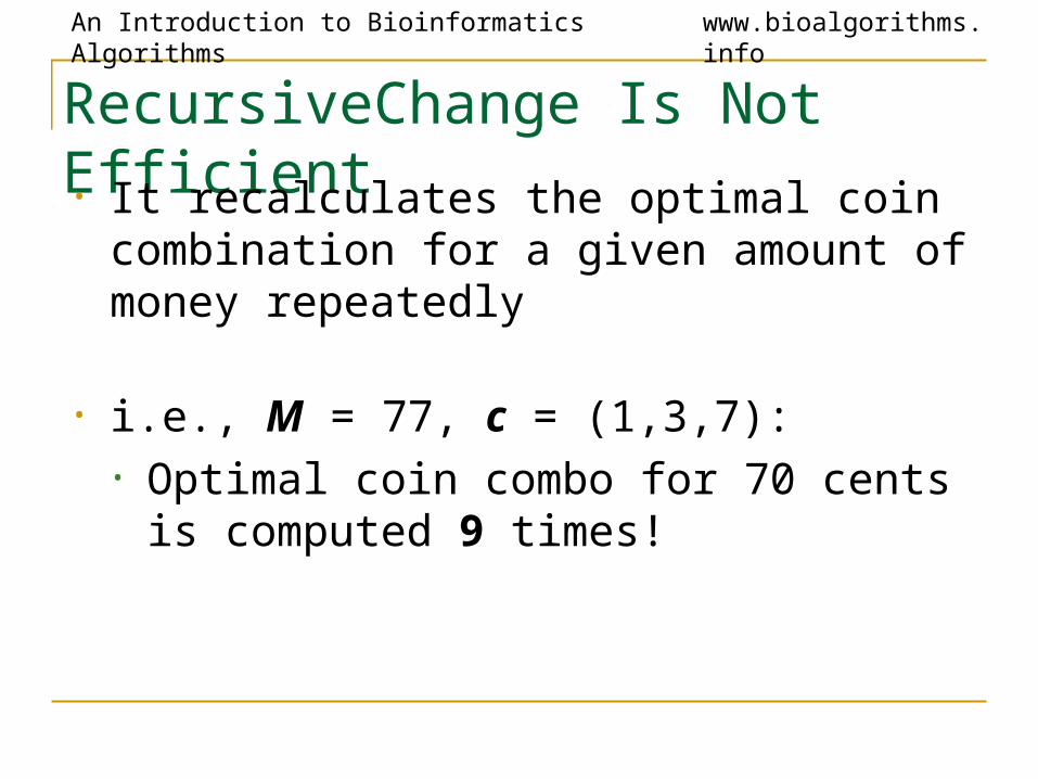
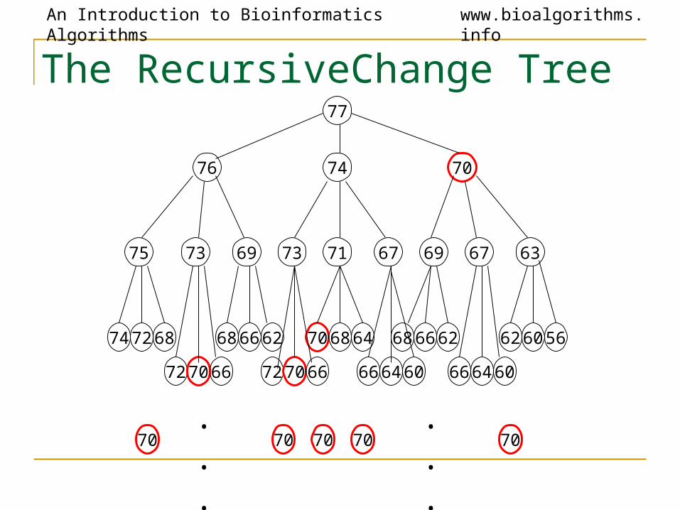
RecursiveChange Is Not Efficient• It recalculates the optimal coin combination
for a given amount of money repeatedly
• i.e., M = 77, c = (1,3,7):• Optimal coin combo for 70 cents is
computed 9 times!
An Introduction to Bioinformatics Algorithms www.bioalgorithms.info
The RecursiveChange Tree
74
77
76 70
75 73 69 73 71 67 69 67 63
74 72 68
72 70 66
68 66 62
72 70 66
70 68 64
66 64 60
68 66 62
66 64 60
62 60 56
. . . . . .70 70 70 7070
An Introduction to Bioinformatics Algorithms www.bioalgorithms.info
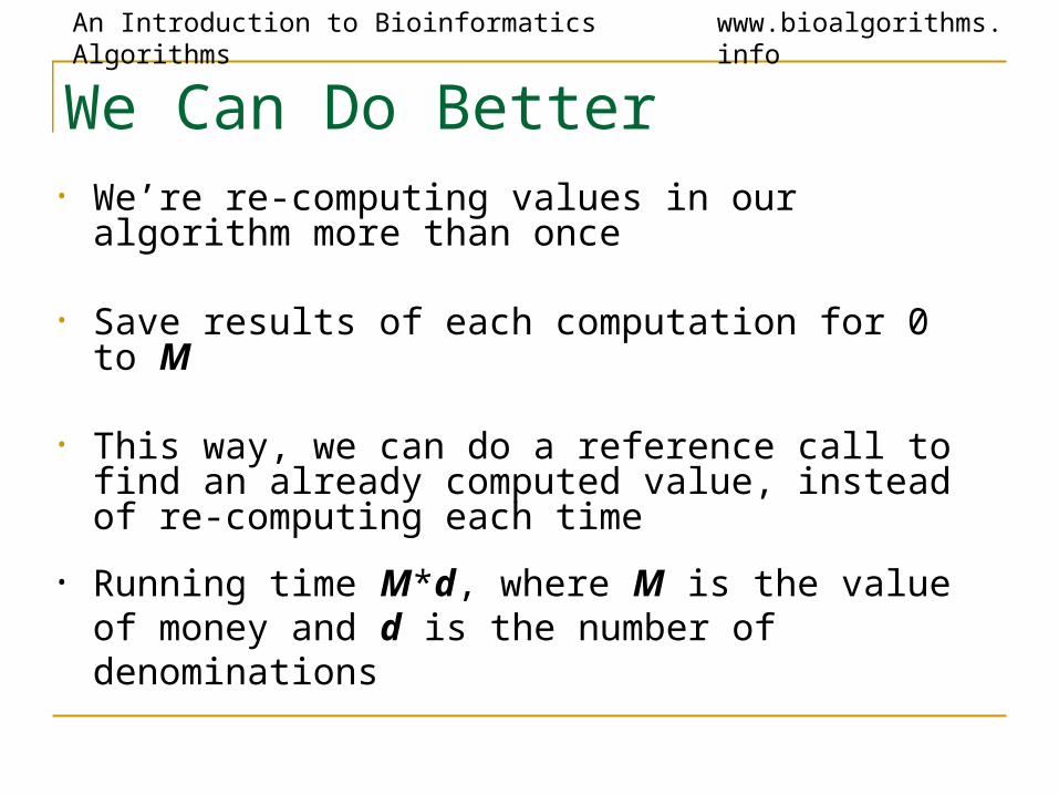
We Can Do Better• We’re re-computing values in our algorithm more
than once
• Save results of each computation for 0 to M
• This way, we can do a reference call to find an already computed value, instead of re-computing each time
• Running time M*d, where M is the value of money and d is the number of denominations
An Introduction to Bioinformatics Algorithms www.bioalgorithms.info
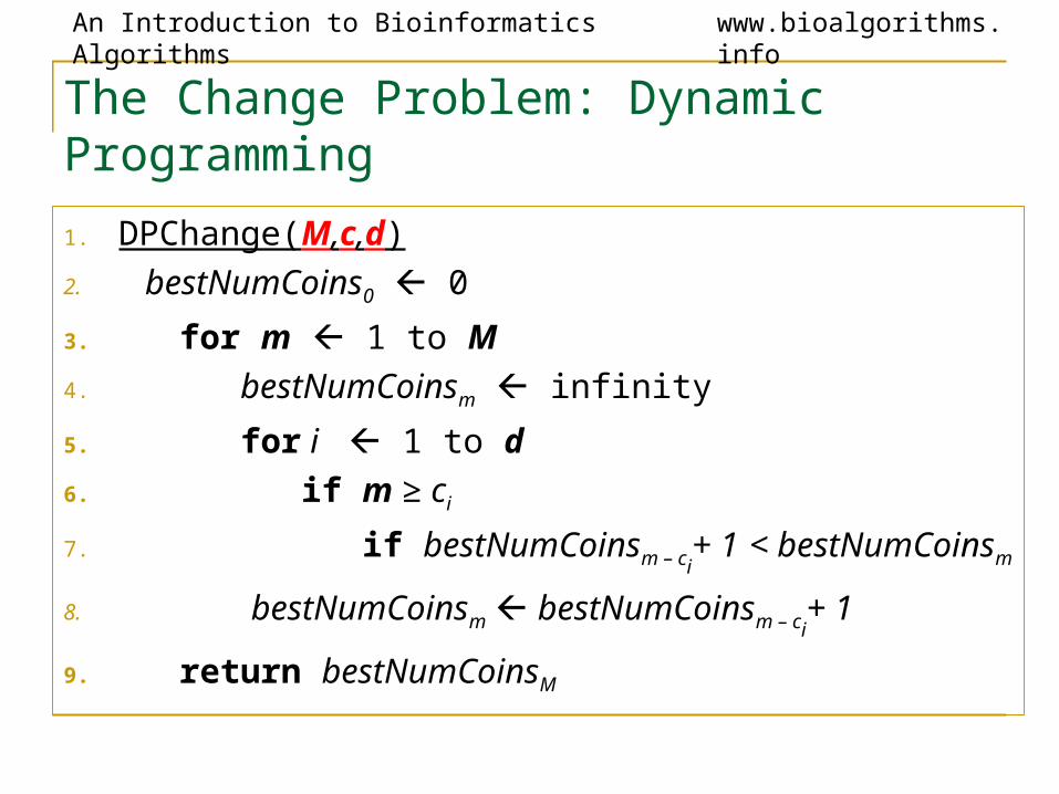
The Change Problem: Dynamic Programming
1. DPChange(M,c,d)2. bestNumCoins0 0
3. for m 1 to M4. bestNumCoinsm infinity
5. for i 1 to d6. if m ≥ ci
7. if bestNumCoinsm – ci+ 1 < bestNumCoinsm
8. bestNumCoinsm bestNumCoinsm – ci+ 1
9. return bestNumCoinsM
An Introduction to Bioinformatics Algorithms www.bioalgorithms.info
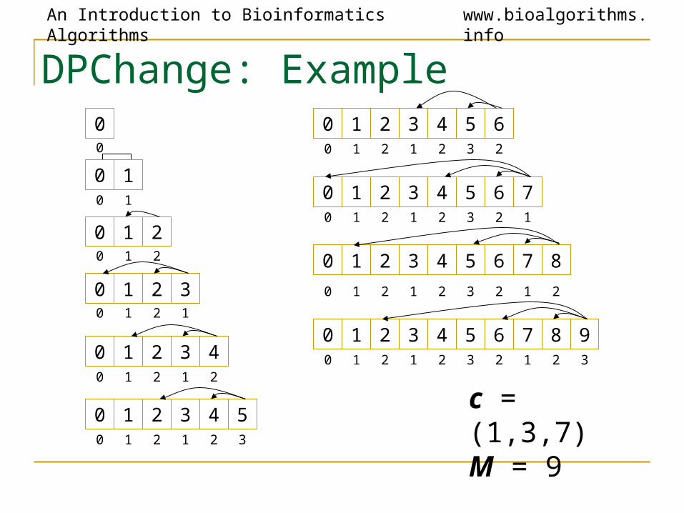
DPChange: Example0
0 1
0 1 2
0 1 2 3
0 1 2 3 4
0 1 2 3 4 5
0 1 2 3 4 5 6
0 1 2 3 4 5 6 7
0 1 2 3 4 5 6 7 8
0 1 2 3 4 5 6 7 8 9
0 1
0
0 1 2
0 1 2 1
0 1 2 1 2
0 1 2 1 2 3
0 1 2 1 2 3 2
0 1 2 1 2 3 2 1
0 1 2 1 2 3 2 1 2
0 1 2 1 2 3 2 1 2 3
c = (1,3,7)M = 9
An Introduction to Bioinformatics Algorithms www.bioalgorithms.info
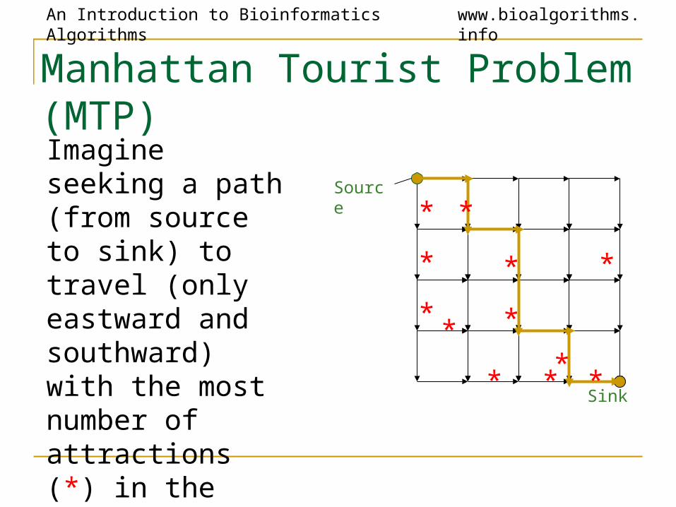
Manhattan Tourist Problem (MTP)Imagine seeking a path (from source to sink) to travel (only eastward and southward) with the most number of attractions (*) in the Manhattan grid Sink
*
*
*
*
*
**
* *
*
*
Source
*
An Introduction to Bioinformatics Algorithms www.bioalgorithms.info
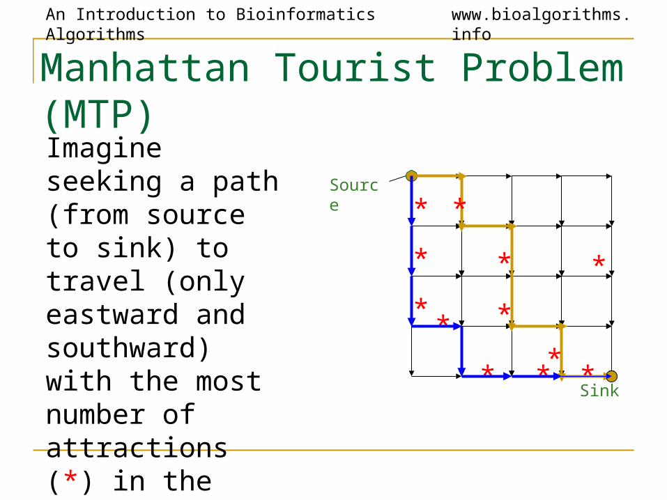
Manhattan Tourist Problem (MTP)Imagine seeking a path (from source to sink) to travel (only eastward and southward) with the most number of attractions (*) in the Manhattan grid Sink
*
*
*
*
*
**
* *
*
*
Source
*
An Introduction to Bioinformatics Algorithms www.bioalgorithms.info
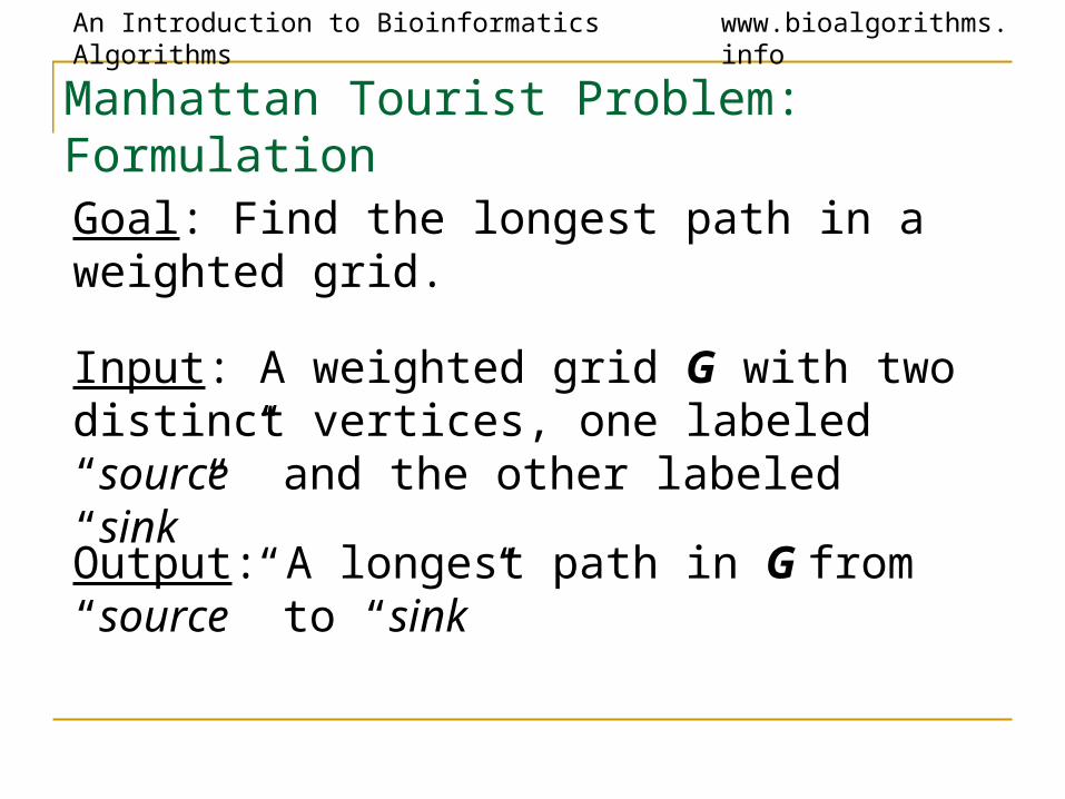
Manhattan Tourist Problem: Formulation
Goal: Find the longest path in a weighted grid.
Input: A weighted grid G with two distinct vertices, one labeled “source” and the other labeled “sink”
Output: A longest path in G from “source” to “sink”
An Introduction to Bioinformatics Algorithms www.bioalgorithms.info
MTP: An Example
3 2 4
0 7 3
3 3 0
1 3 2
4
4
5
6
4
6
5
5
8
2
2
5
0 1 2 3
0
1
2
3
j coordinatei c
oor
dina
te
13
source
sink
4
3 2 4 0
1 0 2 4 3
3
1
1
2
2
2
419
95
15
23
0
20
3
4
An Introduction to Bioinformatics Algorithms www.bioalgorithms.info
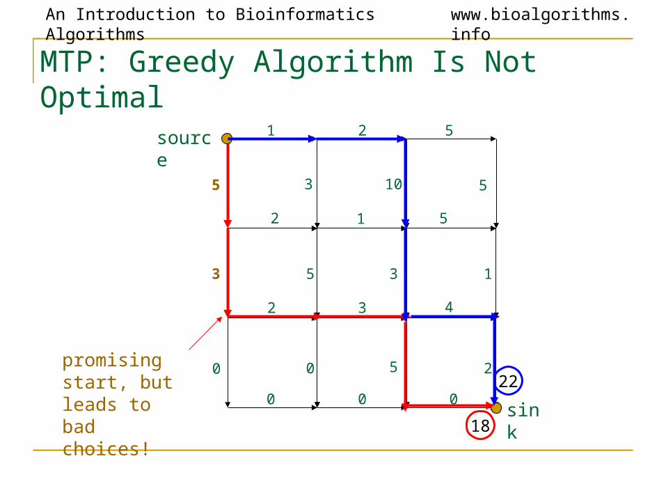
MTP: Greedy Algorithm Is Not Optimal
1 2 5
2 1 5
2 3 4
0 0 0
5
3
0
3
5
0
10
3
5
5
1
2promising start, but leads to bad choices!
source
sink18
22
An Introduction to Bioinformatics Algorithms www.bioalgorithms.info
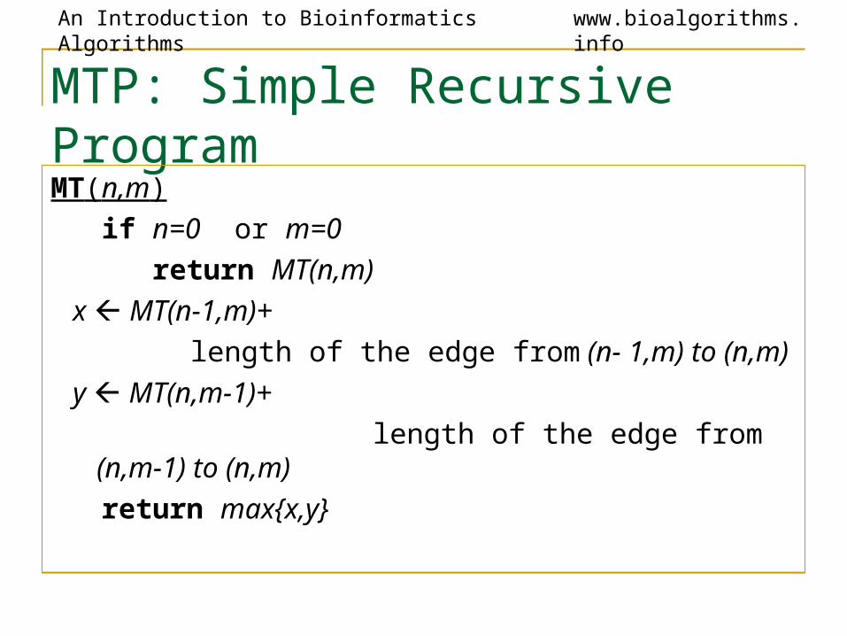
MTP: Simple Recursive ProgramMT(n,m) if n=0 or m=0 return MT(n,m) x MT(n-1,m)+ length of the edge from (n- 1,m) to
(n,m) y MT(n,m-1)+ length of the edge from (n,m-1) to (n,m) return max{x,y}
An Introduction to Bioinformatics Algorithms www.bioalgorithms.info
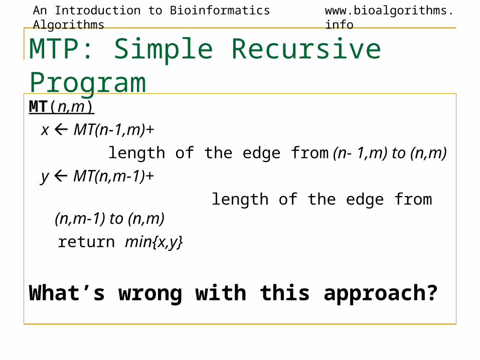
MTP: Simple Recursive ProgramMT(n,m) x MT(n-1,m)+ length of the edge from (n- 1,m) to
(n,m) y MT(n,m-1)+ length of the edge from (n,m-1) to (n,m) return min{x,y}
What’s wrong with this approach?
An Introduction to Bioinformatics Algorithms www.bioalgorithms.info
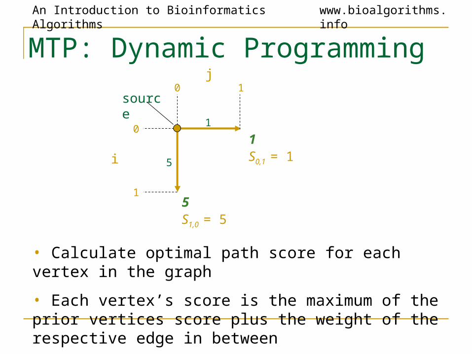
1
5
0 1
0
1
i
source
1
5S1,0 = 5
S0,1 = 1
• Calculate optimal path score for each vertex in the graph
• Each vertex’s score is the maximum of the prior vertices score plus the weight of the respective edge in between
MTP: Dynamic Programmingj
An Introduction to Bioinformatics Algorithms www.bioalgorithms.info
MTP: Dynamic Programming (cont’d)
1 2
5
3
0 1 2
0
1
2
source
1 3
5
8
4
S2,0 = 8
i
S1,1 = 4
S0,2 = 33
-5
j
An Introduction to Bioinformatics Algorithms www.bioalgorithms.info
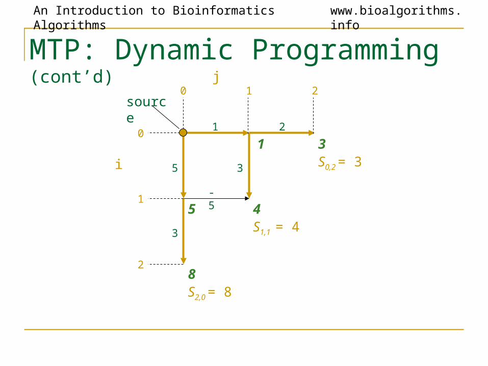
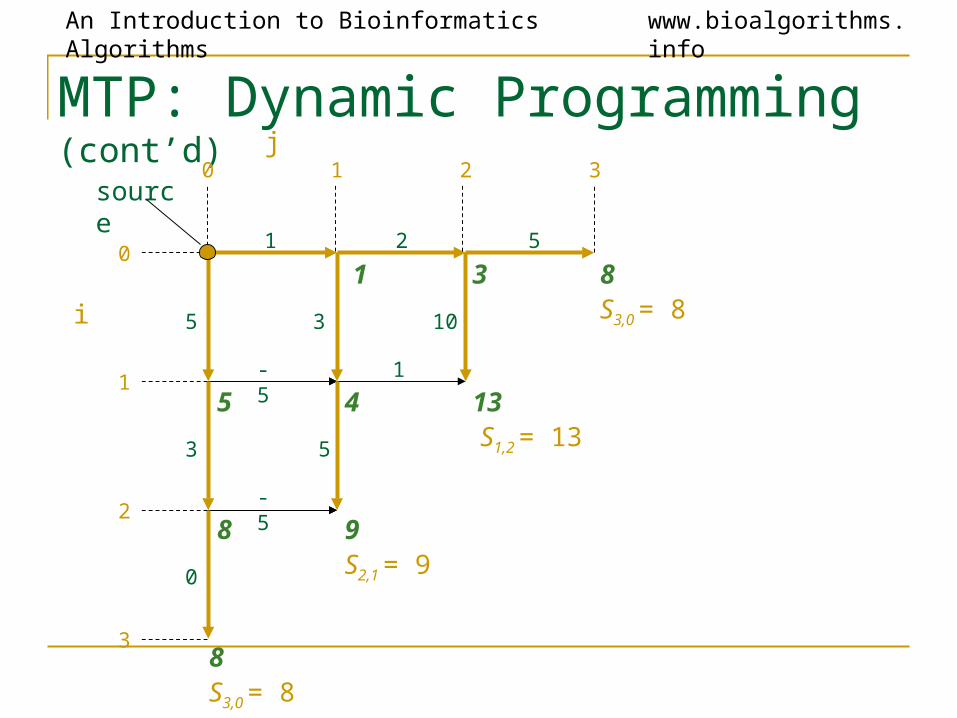
MTP: Dynamic Programming (cont’d)
1 2
5
3
0 1 2 3
0
1
2
3
i
source
1 3
5
8
8
4
0
5
8
103
5
-5
9
131-5
S3,0 = 8
S2,1 = 9
S1,2 = 13
S3,0 = 8
j
An Introduction to Bioinformatics Algorithms www.bioalgorithms.info
MTP: Dynamic Programming (cont’d)
greedy alg. fails!
1 2 5
-5 1 -5
-5 3
0
5
3
0
3
5
0
10
-3
-5
0 1 2 3
0
1
2
3
i
source
1 3 8
5
8
8
4
9
13 8
9
12
S3,1 = 9
S2,2 = 12
S1,3 = 8
j
An Introduction to Bioinformatics Algorithms www.bioalgorithms.info
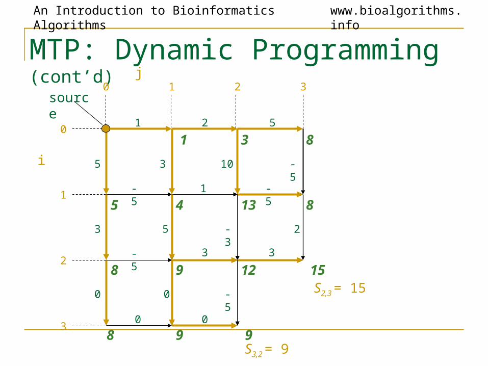
MTP: Dynamic Programming (cont’d)
1 2 5
-5 1 -5
-5 3 3
0 0
5
3
0
3
5
0
10
-3
-5
-5
2
0 1 2 3
0
1
2
3
i
source
1 3 8
5
8
8
4
9
13 8
12
9
15
9
j
S3,2 = 9
S2,3 = 15
An Introduction to Bioinformatics Algorithms www.bioalgorithms.info
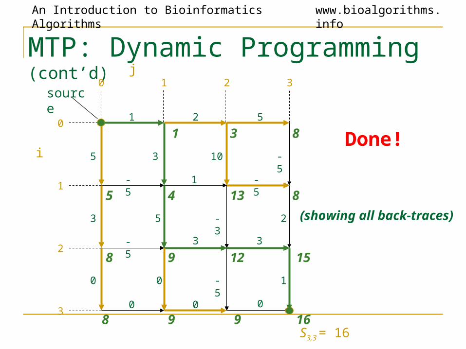
MTP: Dynamic Programming (cont’d)
1 2 5
-5 1 -5
-5 3 3
0 0
5
3
0
3
5
0
10
-3
-5
-5
2
0 1 2 3
0
1
2
3
i
source
1 3 8
5
8
8
4
9
13 8
12
9
15
9
j
0
1
16S3,3 = 16
(showing all back-traces)
Done!
An Introduction to Bioinformatics Algorithms www.bioalgorithms.info
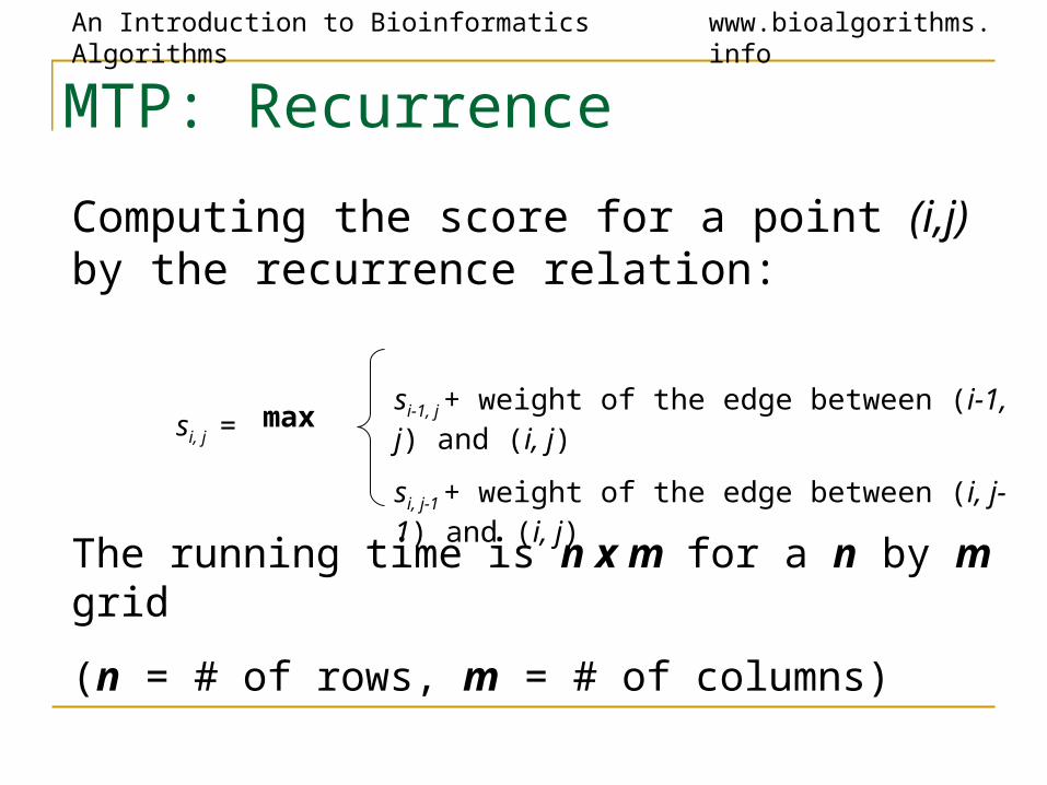
MTP: Recurrence
Computing the score for a point (i,j) by the recurrence relation:
si, j = max si-1, j + weight of the edge between (i-1, j) and (i, j)
si, j-1 + weight of the edge between (i, j-1) and (i, j)
The running time is n x m for a n by m grid
(n = # of rows, m = # of columns)
An Introduction to Bioinformatics Algorithms www.bioalgorithms.info
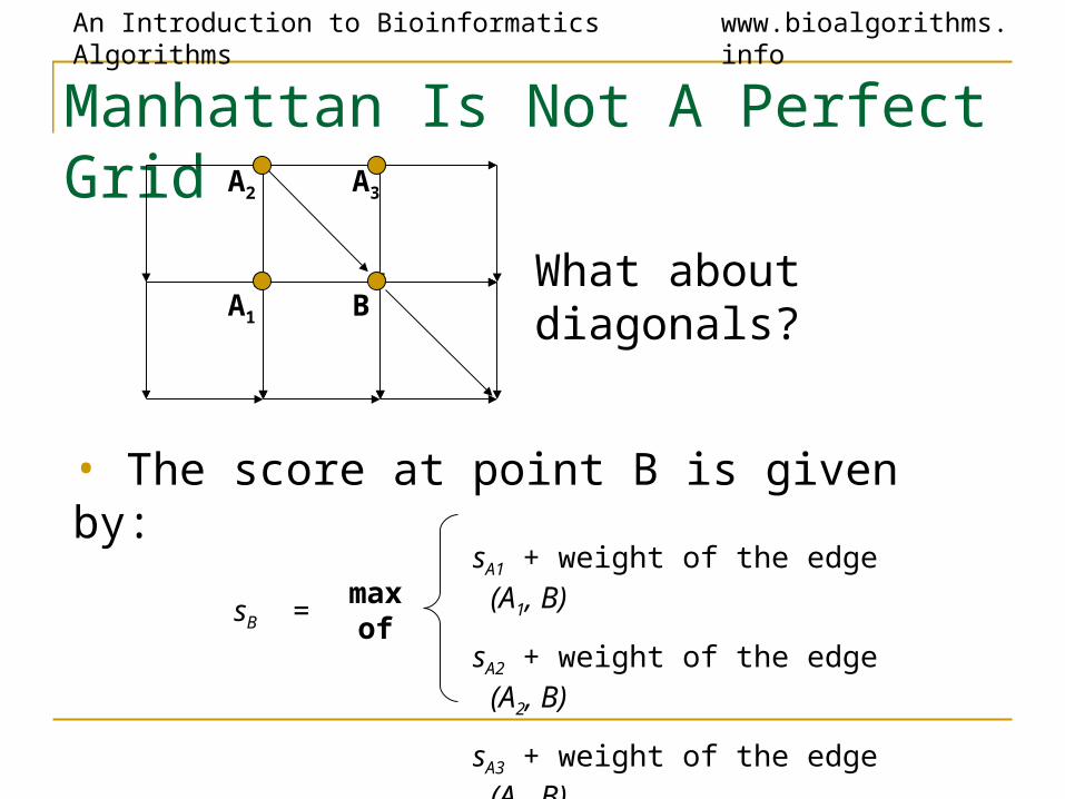
Manhattan Is Not A Perfect Grid
What about diagonals?
• The score at point B is given by:
sB =max of
sA1 + weight of the edge (A1, B)
sA2 + weight of the edge (A2, B)
sA3 + weight of the edge (A3, B)
B
A3
A1
A2
An Introduction to Bioinformatics Algorithms www.bioalgorithms.info
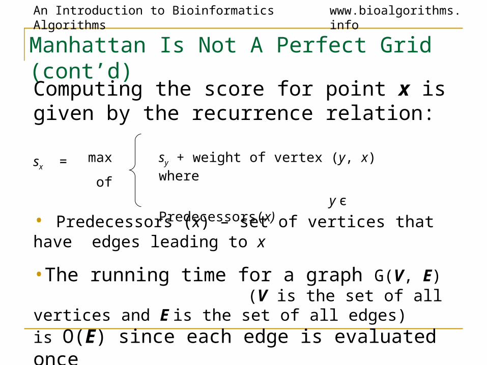
Manhattan Is Not A Perfect Grid (cont’d)
Computing the score for point x is given by the recurrence relation:
sx = max
of
sy + weight of vertex (y, x) where
y є Predecessors(x)
• Predecessors (x) – set of vertices that have edges leading to x
•The running time for a graph G(V, E) (V is the set of all vertices and E is the set of all edges) is O(E) since each edge is evaluated once
An Introduction to Bioinformatics Algorithms www.bioalgorithms.info
Traveling in the Grid•The only hitch is that one must decide on the order in which visit the vertices
•By the time the vertex x is analyzed, the values sy for all its predecessors y should be computed – otherwise we are in trouble.
•We need to traverse the vertices in some order
•Try to find such order for a directed cycle
???
An Introduction to Bioinformatics Algorithms www.bioalgorithms.info
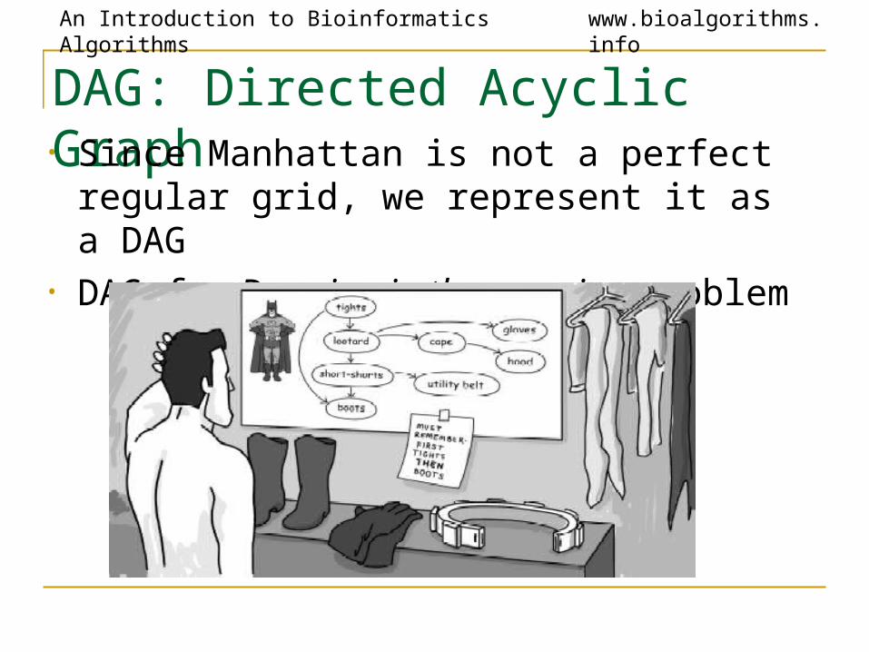
DAG: Directed Acyclic Graph• Since Manhattan is not a perfect regular grid,
we represent it as a DAG • DAG for Dressing in the morning problem
An Introduction to Bioinformatics Algorithms www.bioalgorithms.info
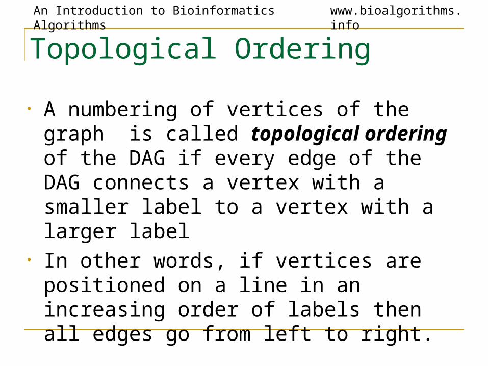
Topological Ordering
• A numbering of vertices of the graph is called topological ordering of the DAG if every edge of the DAG connects a vertex with a smaller label to a vertex with a larger label
• In other words, if vertices are positioned on a line in an increasing order of labels then all edges go from left to right.
An Introduction to Bioinformatics Algorithms www.bioalgorithms.info
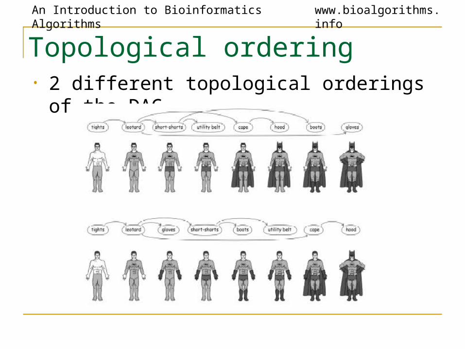
Topological ordering• 2 different topological orderings of the DAG
An Introduction to Bioinformatics Algorithms www.bioalgorithms.info
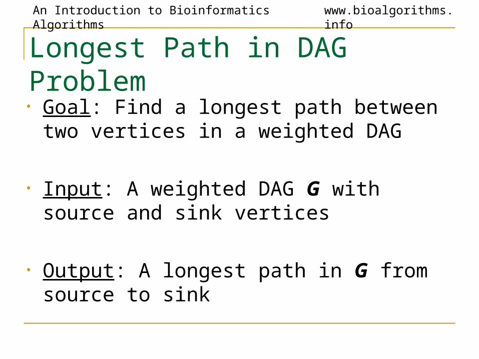
Longest Path in DAG Problem
• Goal: Find a longest path between two vertices in a weighted DAG
• Input: A weighted DAG G with source and sink vertices
• Output: A longest path in G from source to sink
An Introduction to Bioinformatics Algorithms www.bioalgorithms.info
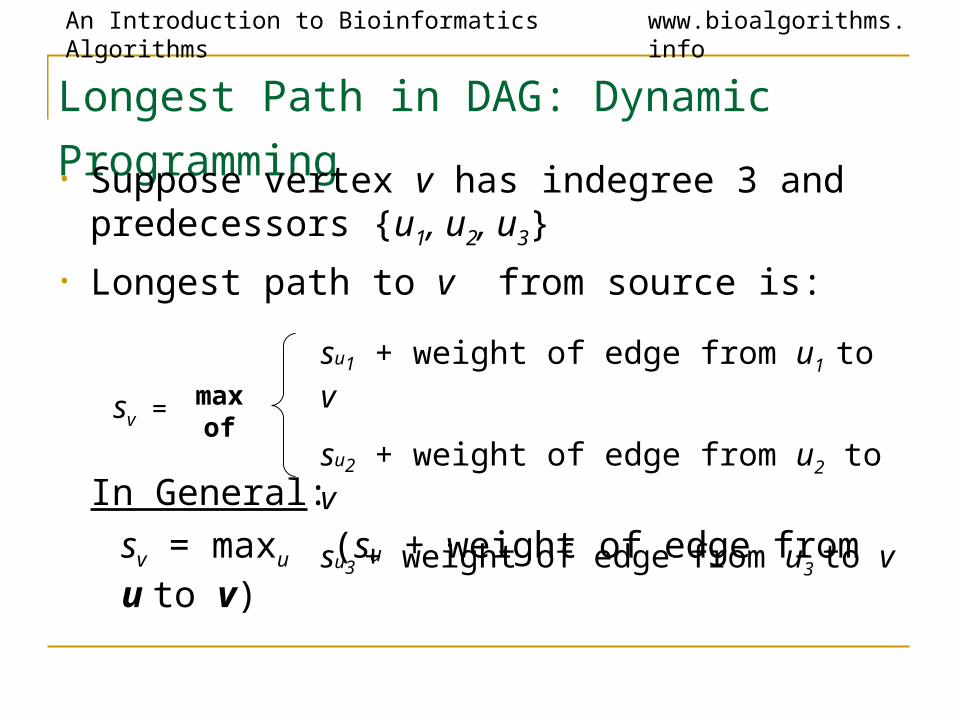
Longest Path in DAG: Dynamic
Programming • Suppose vertex v has indegree 3 and predecessors {u1, u2, u3}
• Longest path to v from source is:
In General:
sv = maxu (su + weight of edge from u to v)
sv =max of
su1 + weight of edge from u1 to v
su2 + weight of edge from u2 to v
su3 + weight of edge from u3 to v
An Introduction to Bioinformatics Algorithms www.bioalgorithms.info
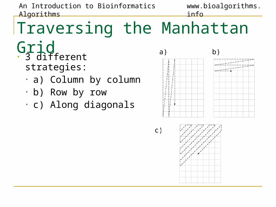
Traversing the Manhattan Grid • 3 different strategies:
• a) Column by column• b) Row by row• c) Along diagonals
a) b)
c)
An Introduction to Bioinformatics Algorithms www.bioalgorithms.info
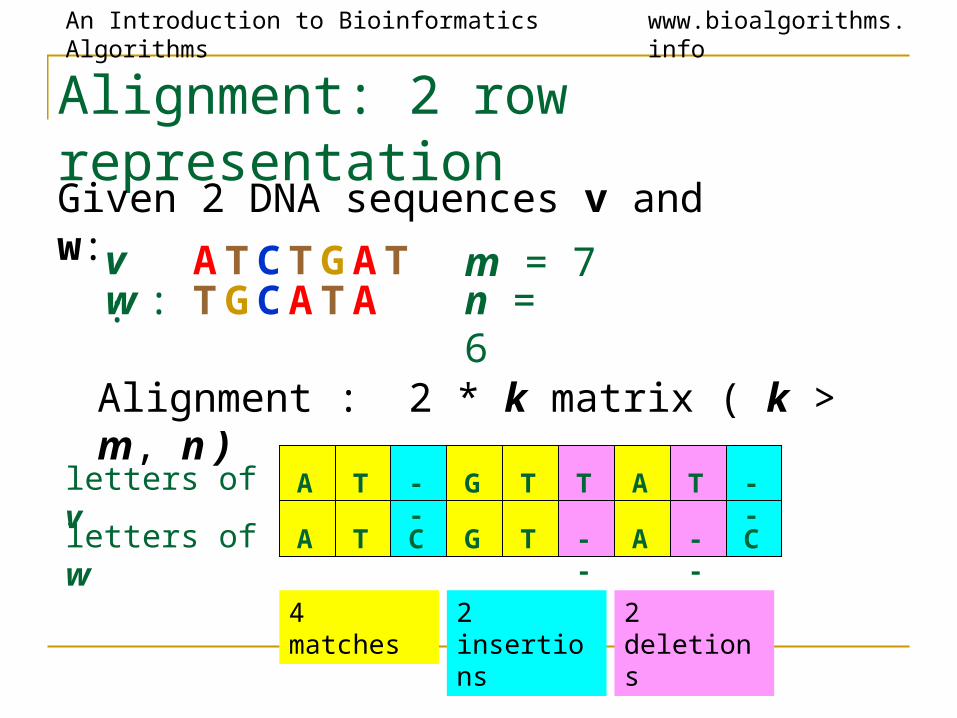
Alignment: 2 row representation
Alignment : 2 * k matrix ( k > m, n )
A T -- G T A T --
A T C G -- A -- C
letters of v
letters of w
T
T
AT CT GATT GCAT A
v :w :
m = 7 n = 6
4 matches 2 insertions 2 deletions
Given 2 DNA sequences v and w:
An Introduction to Bioinformatics Algorithms www.bioalgorithms.info
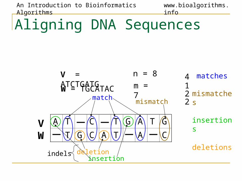
Aligning DNA Sequences
V = ATCTGATGW = TGCATAC
n = 8
m = 7
A T C T G A T G
T G C A T A CV
W
match
deletioninsertion
mismatch
indels
4122
matches mismatches insertions deletions
An Introduction to Bioinformatics Algorithms www.bioalgorithms.info
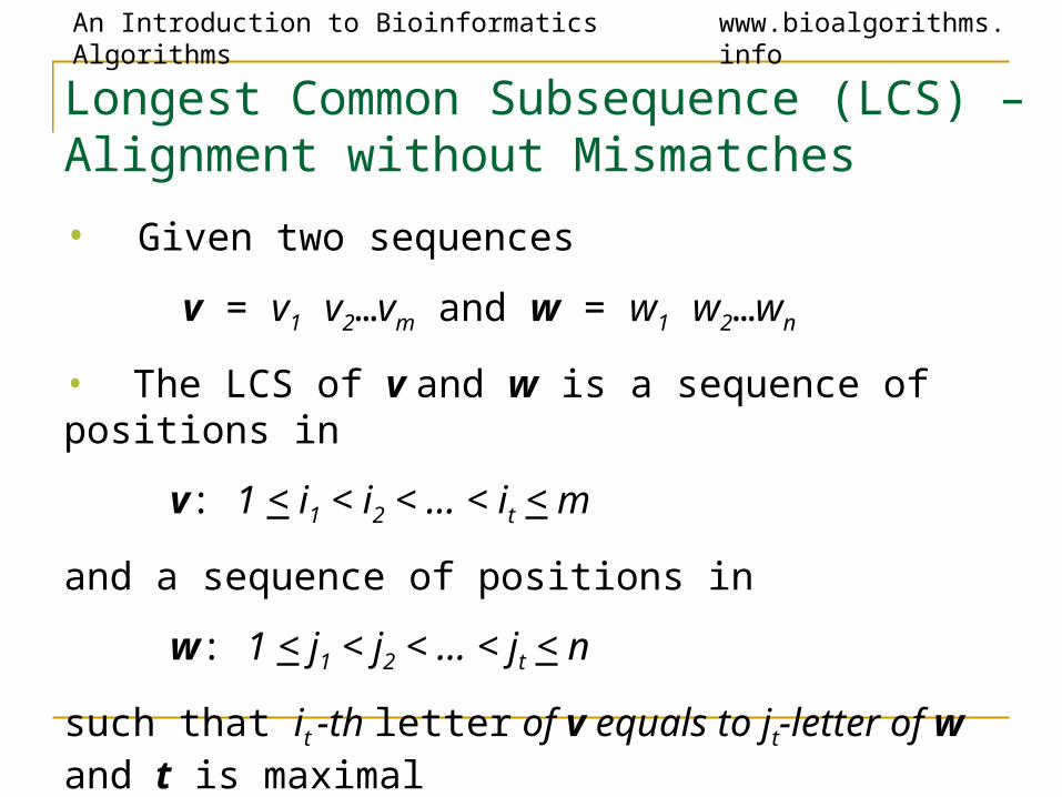
Longest Common Subsequence (LCS) – Alignment without Mismatches
• Given two sequences
v = v1 v2…vm and w = w1 w2…wn
• The LCS of v and w is a sequence of positions in
v: 1 < i1 < i2 < … < it < m
and a sequence of positions in
w: 1 < j1 < j2 < … < jt < n
such that it -th letter of v equals to jt-letter of w and t is maximal
An Introduction to Bioinformatics Algorithms www.bioalgorithms.info
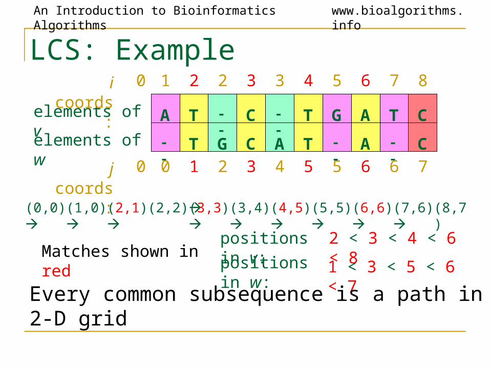
LCS: Example
A T -- C T G A T C
-- T G C T -- A -- C
elements of v
elements of w
--
A1
2
0
1
2
2
3
3
4
3
5
4
5
5
6
6
6
7
7
8
j coords:
i coords:
Matches shown in redpositions in v:
positions in w:
2 < 3 < 4 < 6 < 8
1 < 3 < 5 < 6 < 7
Every common subsequence is a path in 2-D grid
0
0
(0,0)(1,0)(2,1)(2,2)(3,3)(3,4)(4,5)(5,5)(6,6)(7,6)(8,7)
An Introduction to Bioinformatics Algorithms www.bioalgorithms.info
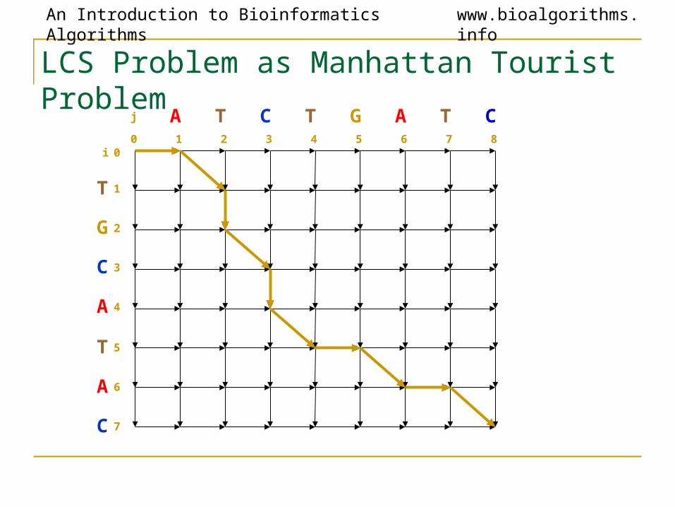
LCS Problem as Manhattan Tourist Problem
T
G
C
A
T
A
C
1
2
3
4
5
6
7
0i
A T C T G A T C0 1 2 3 4 5 6 7 8
j

An Introduction to Bioinformatics Algorithms www.bioalgorithms.info
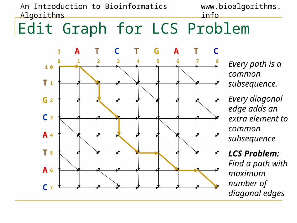
Edit Graph for LCS Problem
T
G
C
A
T
A
C
1
2
3
4
5
6
7
0i
A T C T G A T C0 1 2 3 4 5 6 7 8
j
An Introduction to Bioinformatics Algorithms www.bioalgorithms.info
Edit Graph for LCS Problem
T
G
C
A
T
A
C
1
2
3
4
5
6
7
0i
A T C T G A T C0 1 2 3 4 5 6 7 8
j
Every path is a common subsequence.
Every diagonal edge adds an extra element to common subsequence
LCS Problem: Find a path with maximum number of diagonal edges
An Introduction to Bioinformatics Algorithms www.bioalgorithms.info
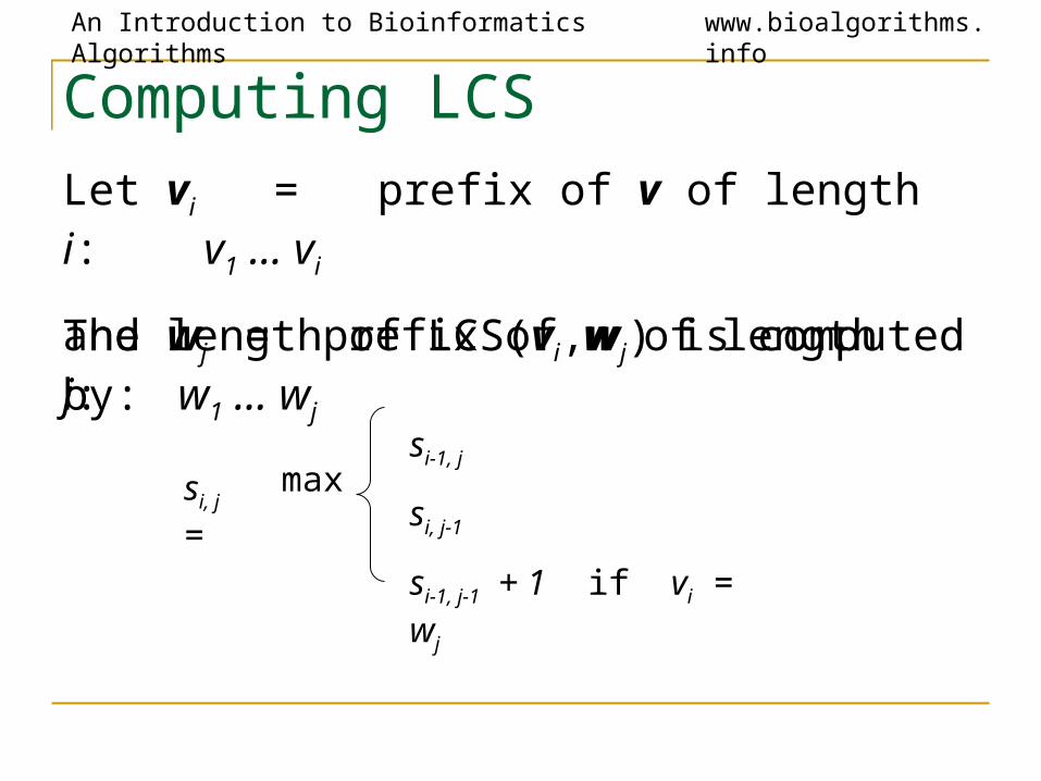
Computing LCSLet vi = prefix of v of length i: v1 … vi
and wj = prefix of w of length j: w1 … wj
The length of LCS(vi,wj) is computed by:
si, j = maxsi-1, j
si, j-1
si-1, j-1 + 1 if vi = wj
An Introduction to Bioinformatics Algorithms www.bioalgorithms.info
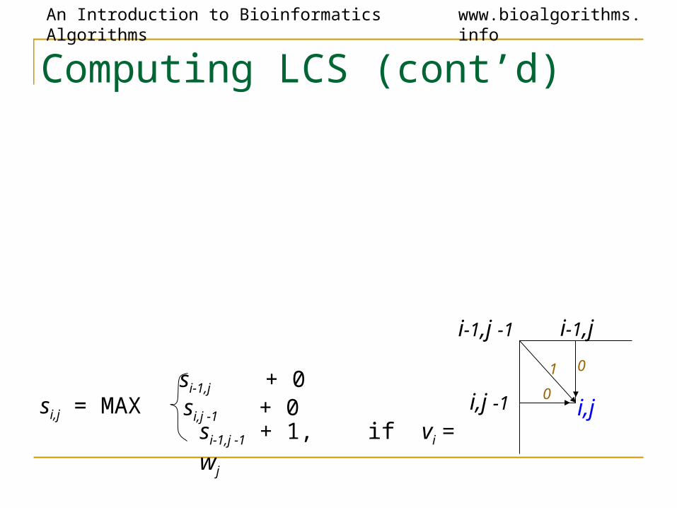
Computing LCS (cont’d)
si,j = MAX si-1,j + 0 si,j -1 + 0 si-1,j -1 + 1, if vi = wj
i,j
i-1,j
i,j -1
i-1,j -1
1 0
0
An Introduction to Bioinformatics Algorithms www.bioalgorithms.info
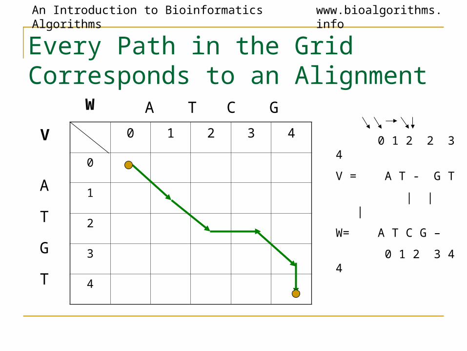
Every Path in the Grid Corresponds to an Alignment
0 1 2 3 4
0
1
2
3
4
W A T C G
A
T
G
T
V
0 1 2 2 3 4
V = A T - G T
| | |
W= A T C G –
0 1 2 3 4 4
An Introduction to Bioinformatics Algorithms www.bioalgorithms.info
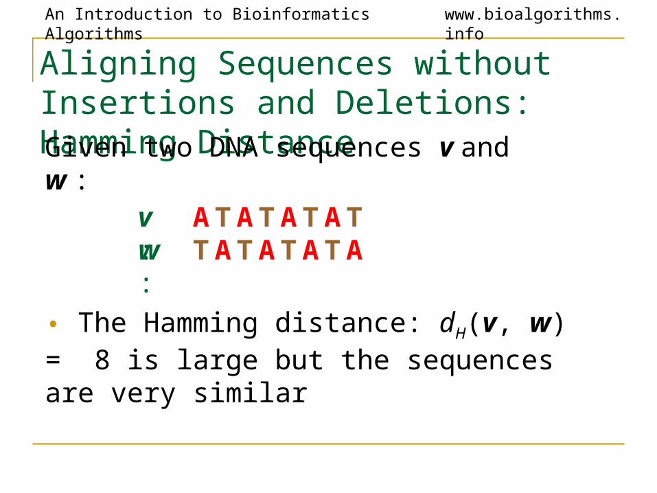
Aligning Sequences without Insertions and Deletions: Hamming DistanceGiven two DNA sequences v and w :
v :
• The Hamming distance: dH(v, w) = 8 is large but the sequences are very similar
AT AT AT ATAT AT AT ATw :
An Introduction to Bioinformatics Algorithms www.bioalgorithms.info
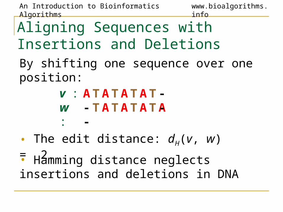
Aligning Sequences with Insertions and Deletions
v : AT AT AT ATAT AT AT ATw : ----
By shifting one sequence over one position:
• The edit distance: dH(v, w) = 2.
• Hamming distance neglects insertions and deletions in DNA
An Introduction to Bioinformatics Algorithms www.bioalgorithms.info
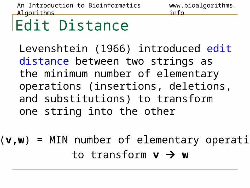
Edit Distance
Levenshtein (1966) introduced edit distance between two strings as the minimum number of elementary operations (insertions, deletions, and substitutions) to transform one string into the other
d(v,w) = MIN number of elementary operations
to transform v w
An Introduction to Bioinformatics Algorithms www.bioalgorithms.info
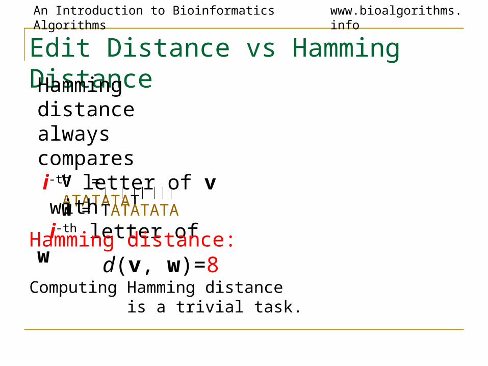
Edit Distance vs Hamming Distance
V = ATATATAT
W = TATATATA
Hamming distance always compares i-th letter of v with i-th letter of w
Hamming distance: d(v, w)=8Computing Hamming distance is a trivial task.

An Introduction to Bioinformatics Algorithms www.bioalgorithms.info
Edit Distance vs Hamming Distance
V = ATATATAT
W = TATATATA
Hamming distance: Edit distance: d(v, w)=8 d(v, w)=2
Computing Hamming distance Computing edit distance
is a trivial task is a non-trivial task
W = TATATATA
Just one shift
Make it all line up
V = - ATATATAT
Hamming distance always compares i-th letter of v with i-th letter of w
Edit distance may compare i-th letter of v with j-th letter of w
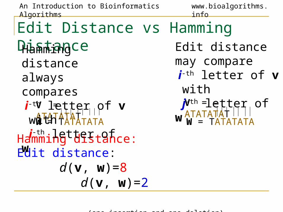
An Introduction to Bioinformatics Algorithms www.bioalgorithms.info
Edit Distance vs Hamming Distance
V = ATATATAT
W = TATATATA
Hamming distance: Edit distance: d(v, w)=8 d(v, w)=2
(one insertion and one deletion)
How to find what j goes with what i ???
W = TATATATA
V = - ATATATAT
Hamming distance always compares i-th letter of v with i-th letter of w
Edit distance may compare i-th letter of v with j-th letter of w
An Introduction to Bioinformatics Algorithms www.bioalgorithms.info
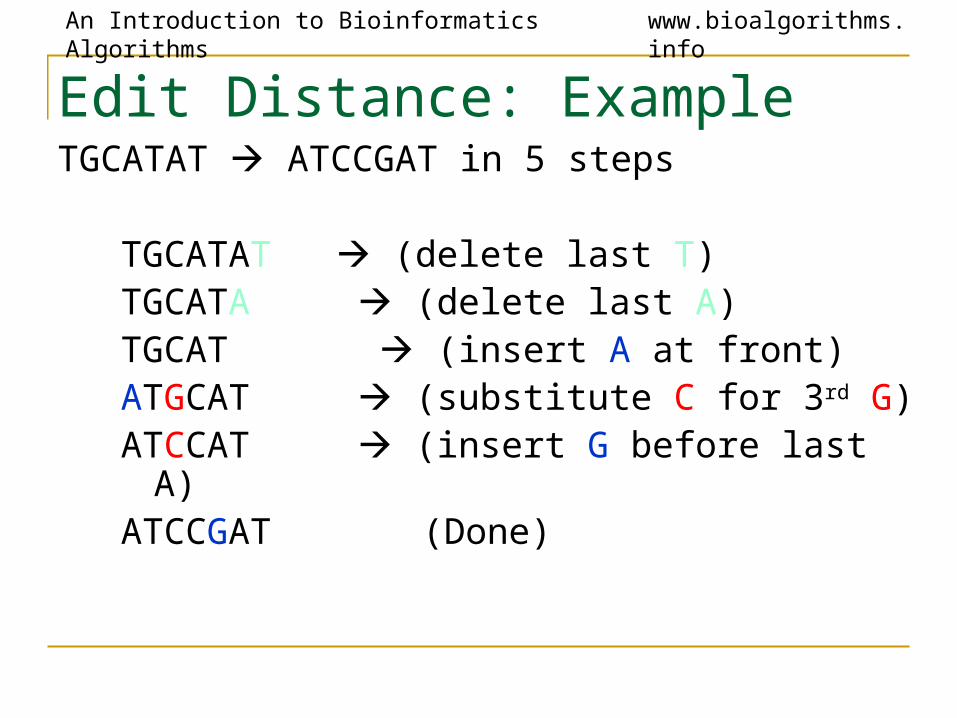
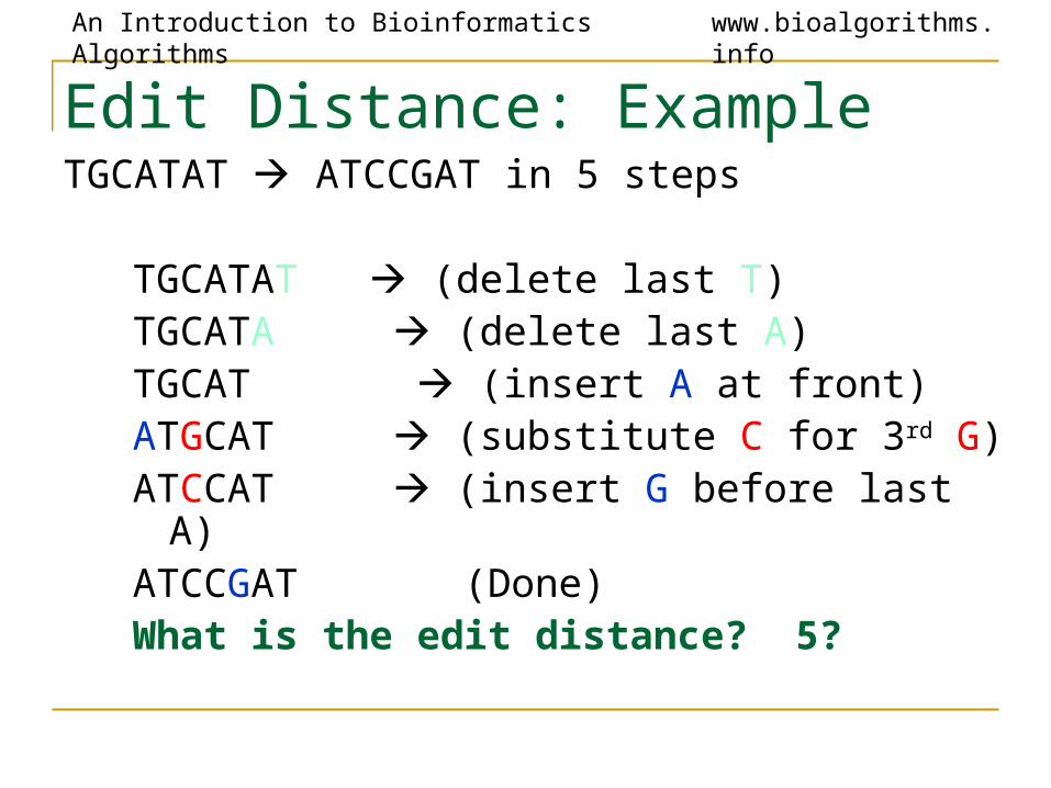
Edit Distance: ExampleTGCATAT ATCCGAT in 5 steps
TGCATAT (delete last T)TGCATA (delete last A)TGCAT (insert A at front)ATGCAT (substitute C for 3rd G)ATCCAT (insert G before last A) ATCCGAT (Done)
An Introduction to Bioinformatics Algorithms www.bioalgorithms.info
Edit Distance: ExampleTGCATAT ATCCGAT in 5 steps
TGCATAT (delete last T)TGCATA (delete last A)TGCAT (insert A at front)ATGCAT (substitute C for 3rd G)ATCCAT (insert G before last A) ATCCGAT (Done)What is the edit distance? 5?
An Introduction to Bioinformatics Algorithms www.bioalgorithms.info
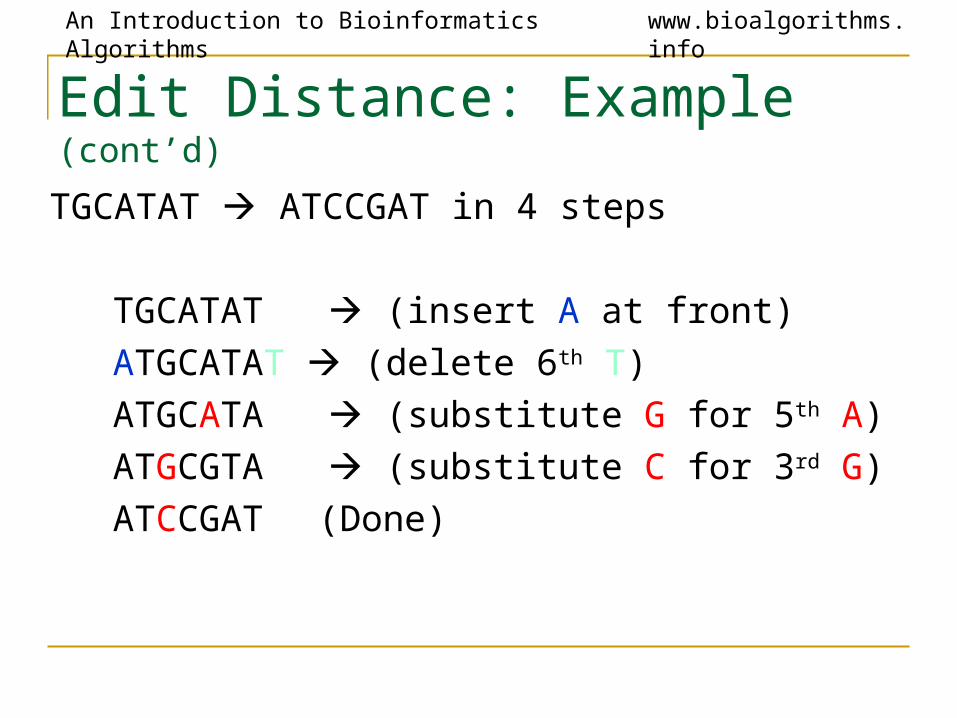
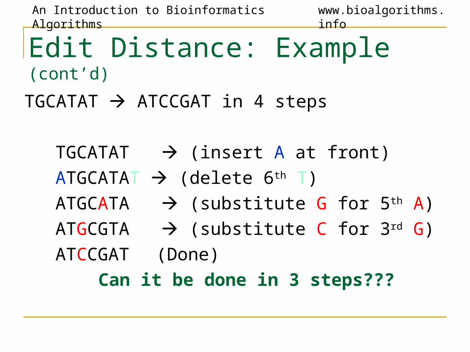
Edit Distance: Example (cont’d)
TGCATAT ATCCGAT in 4 steps
TGCATAT (insert A at front)
ATGCATAT (delete 6th T)
ATGCATA (substitute G for 5th A)
ATGCGTA (substitute C for 3rd G)
ATCCGAT (Done)
An Introduction to Bioinformatics Algorithms www.bioalgorithms.info
Edit Distance: Example (cont’d)
TGCATAT ATCCGAT in 4 steps
TGCATAT (insert A at front)
ATGCATAT (delete 6th T)
ATGCATA (substitute G for 5th A)
ATGCGTA (substitute C for 3rd G)
ATCCGAT (Done)
Can it be done in 3 steps???
An Introduction to Bioinformatics Algorithms www.bioalgorithms.info
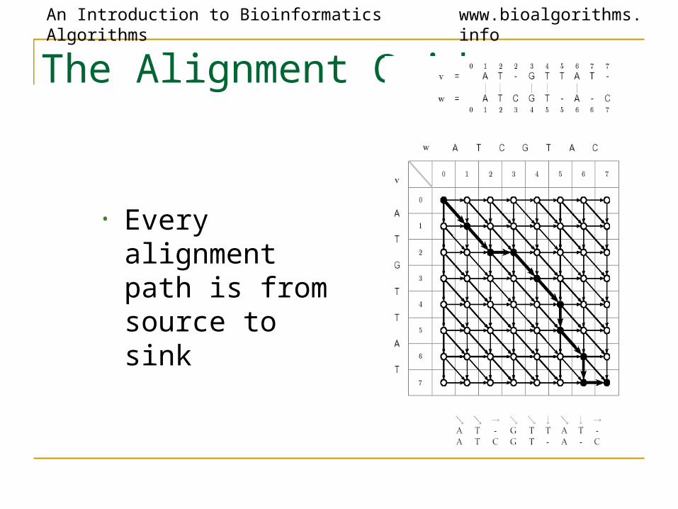
The Alignment Grid
• Every alignment path is from source to sink
An Introduction to Bioinformatics Algorithms www.bioalgorithms.info
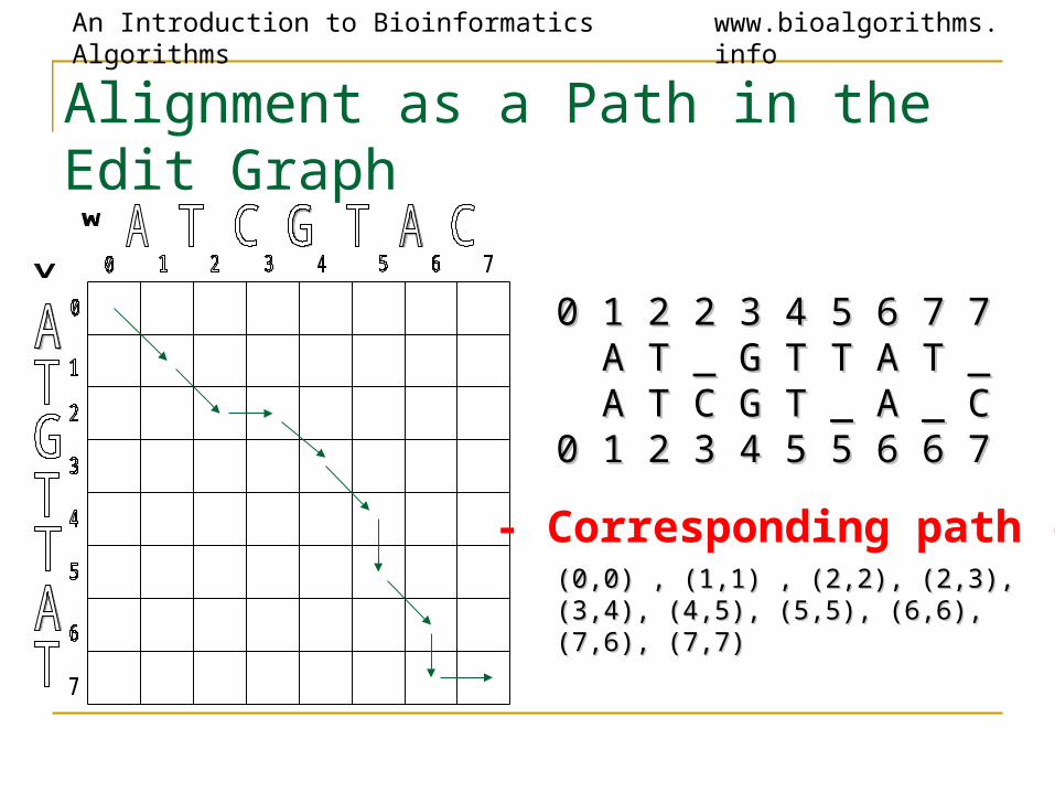
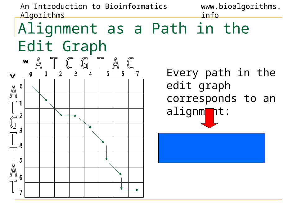
Alignment as a Path in the Edit Graph
0 1 2 2 3 4 5 6 7 70 1 2 2 3 4 5 6 7 7 A T _ G T T A T _A T _ G T T A T _ A T C G T _ A _ CA T C G T _ A _ C0 1 2 3 4 5 5 6 6 7 0 1 2 3 4 5 5 6 6 7
(0,0) , (1,1) , (2,2), (2,3), (0,0) , (1,1) , (2,2), (2,3), (3,4), (4,5), (5,5), (6,6), (3,4), (4,5), (5,5), (6,6), (7,6), (7,7)(7,6), (7,7)
- Corresponding path -
An Introduction to Bioinformatics Algorithms www.bioalgorithms.info
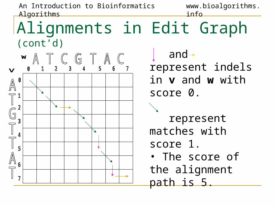
Alignments in Edit Graph (cont’d)
and represent indels in v and w with score 0.
represent matches with score 1.• The score of the alignment path is 5.
An Introduction to Bioinformatics Algorithms www.bioalgorithms.info
Alignment as a Path in the Edit Graph
Every path in the edit graph corresponds to an alignment:
An Introduction to Bioinformatics Algorithms www.bioalgorithms.info
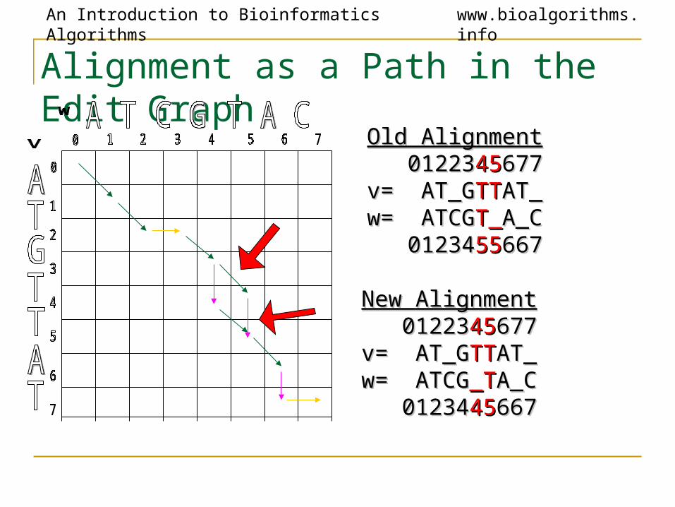
Alignment as a Path in the Edit Graph
Old AlignmentOld Alignment 01223012234545677677v= AT_Gv= AT_GTTTTAT_AT_w= ATCGw= ATCGT_T_A_CA_C 01234012345555667667
New AlignmentNew Alignment 01223012234545677677v= AT_Gv= AT_GTTTTAT_AT_w= ATCGw= ATCG_T_TA_CA_C 01234012344545667667
An Introduction to Bioinformatics Algorithms www.bioalgorithms.info
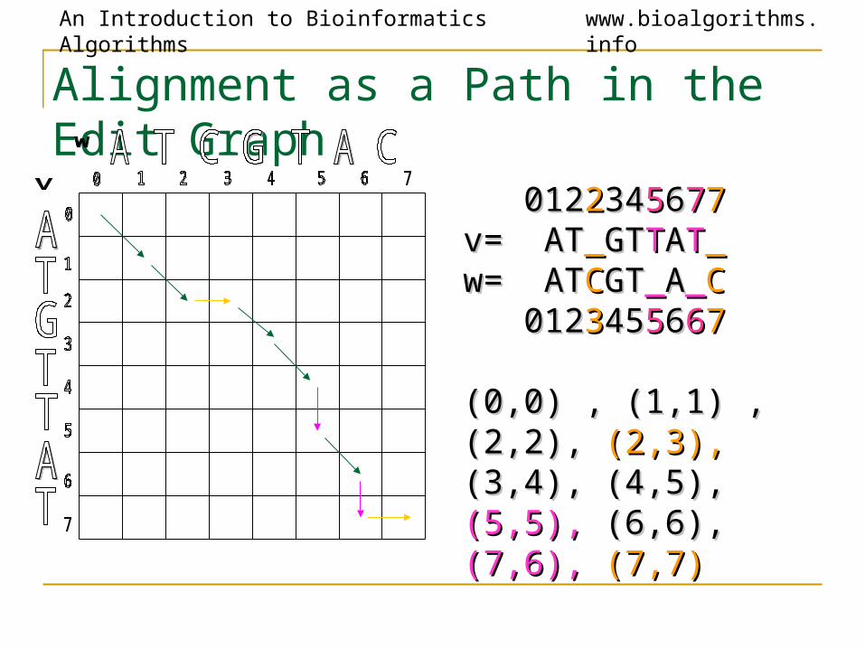
Alignment as a Path in the Edit Graph
01201222343455667777v= ATv= AT__GTGTTTAATT__w= ATw= ATCCGTGT__AA__CC 01201233454555666677
(0,0) , (1,1) , (2,2), (0,0) , (1,1) , (2,2), (2,3),(2,3), (3,4), (4,5), (3,4), (4,5), (5,5),(5,5), (6,6), (6,6), (7,6),(7,6), (7,7)(7,7)

An Introduction to Bioinformatics Algorithms www.bioalgorithms.info
Alignment: Dynamic Programming
si,j = si-1, j-1+1 if vi = wj
max si-1, j
si, j-1
An Introduction to Bioinformatics Algorithms www.bioalgorithms.info
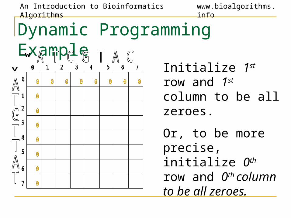
Dynamic Programming Example
Initialize 1st row and 1st column to be all zeroes.
Or, to be more precise, initialize 0th row and 0th column to be all zeroes.
An Introduction to Bioinformatics Algorithms www.bioalgorithms.info
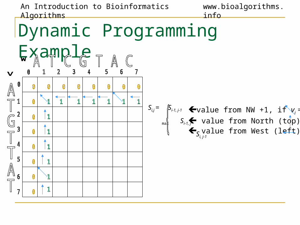
Dynamic Programming Example
Si,j = Si-1, j-1
max Si-1, j
Si, j-1
value from NW +1, if vi = wj
value from North (top) value from West (left)
An Introduction to Bioinformatics Algorithms www.bioalgorithms.info
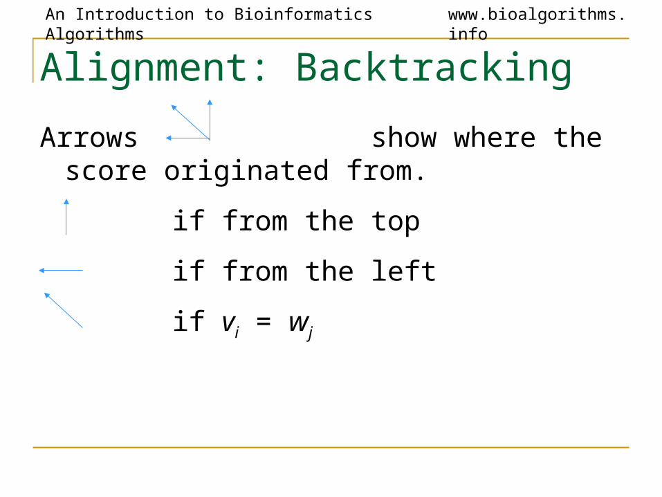
Alignment: Backtracking
Arrows show where the score originated from.
if from the top
if from the left
if vi = wj
An Introduction to Bioinformatics Algorithms www.bioalgorithms.info
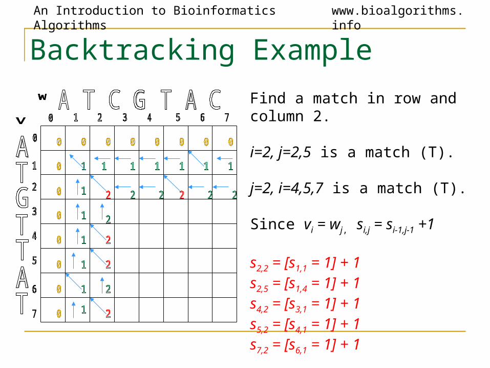
Backtracking Example
Find a match in row and column 2.
i=2, j=2,5 is a match (T).
j=2, i=4,5,7 is a match (T).
Since vi = wj, si,j = si-1,j-1 +1
s2,2 = [s1,1 = 1] + 1 s2,5 = [s1,4 = 1] + 1s4,2 = [s3,1 = 1] + 1s5,2 = [s4,1 = 1] + 1s7,2 = [s6,1 = 1] + 1
An Introduction to Bioinformatics Algorithms www.bioalgorithms.info
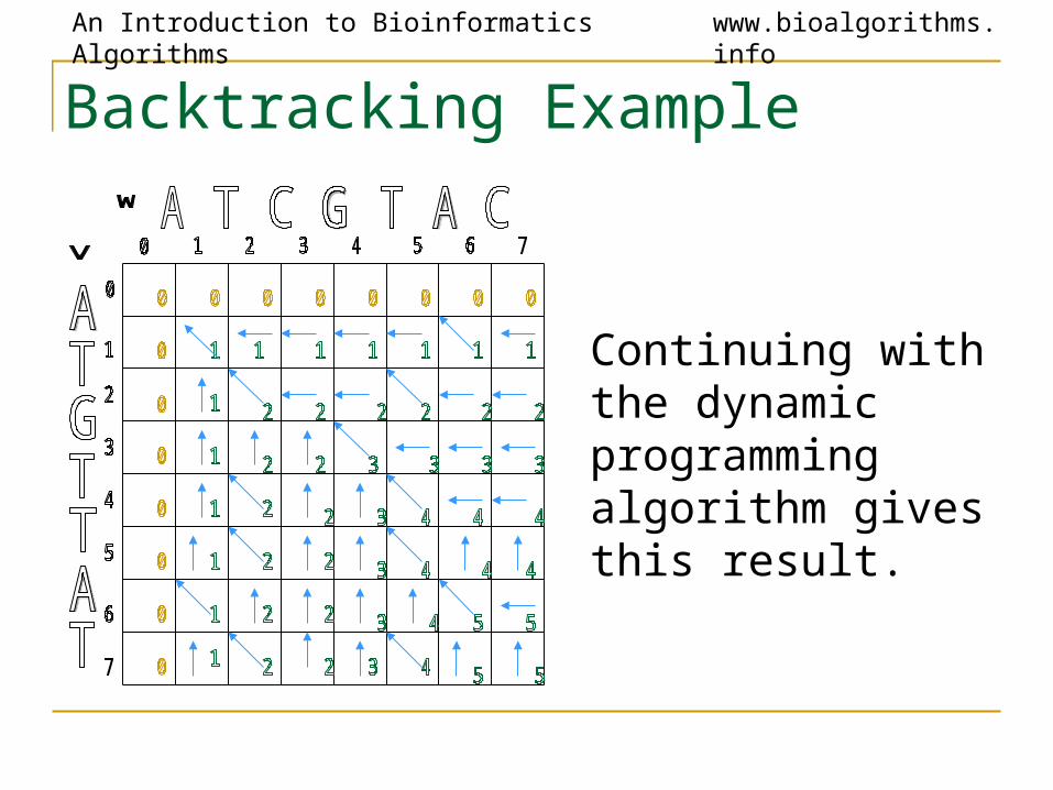
Backtracking Example
Continuing with the dynamic programming algorithm gives this result.
An Introduction to Bioinformatics Algorithms www.bioalgorithms.info
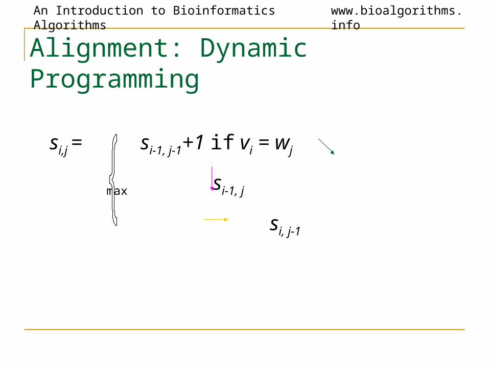
Alignment: Dynamic Programming
si,j = si-1, j-1+1 if vi = wj
max si-1, j
si, j-1
An Introduction to Bioinformatics Algorithms www.bioalgorithms.info
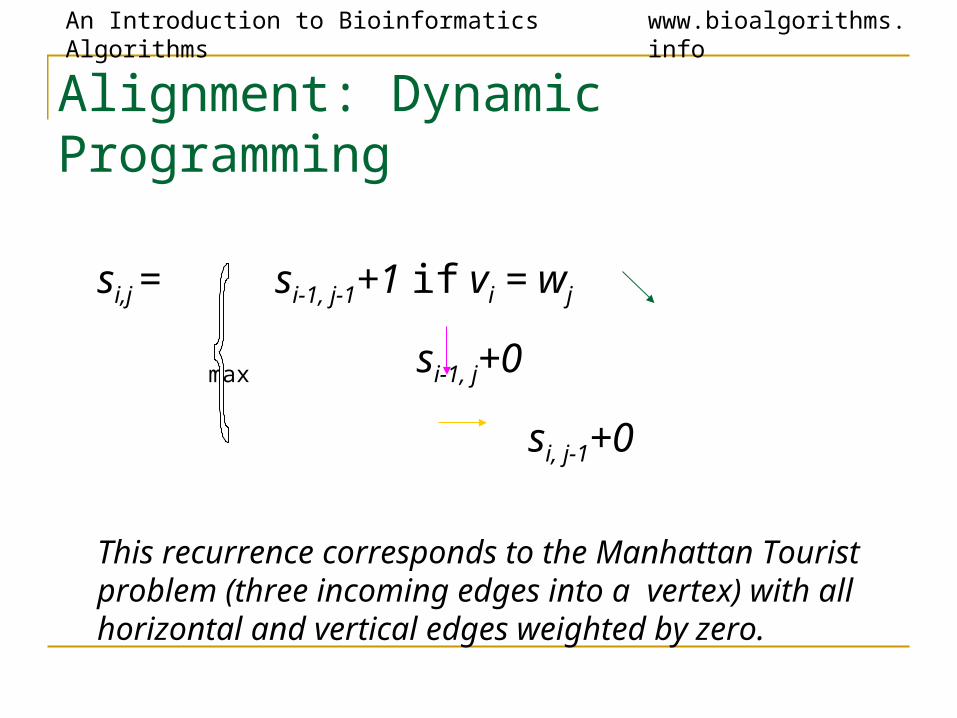
Alignment: Dynamic Programming
si,j = si-1, j-1+1 if vi = wj
max si-1, j+0
si, j-1+0
This recurrence corresponds to the Manhattan Tourist problem (three incoming edges into a vertex) with all horizontal and vertical edges weighted by zero.
An Introduction to Bioinformatics Algorithms www.bioalgorithms.info
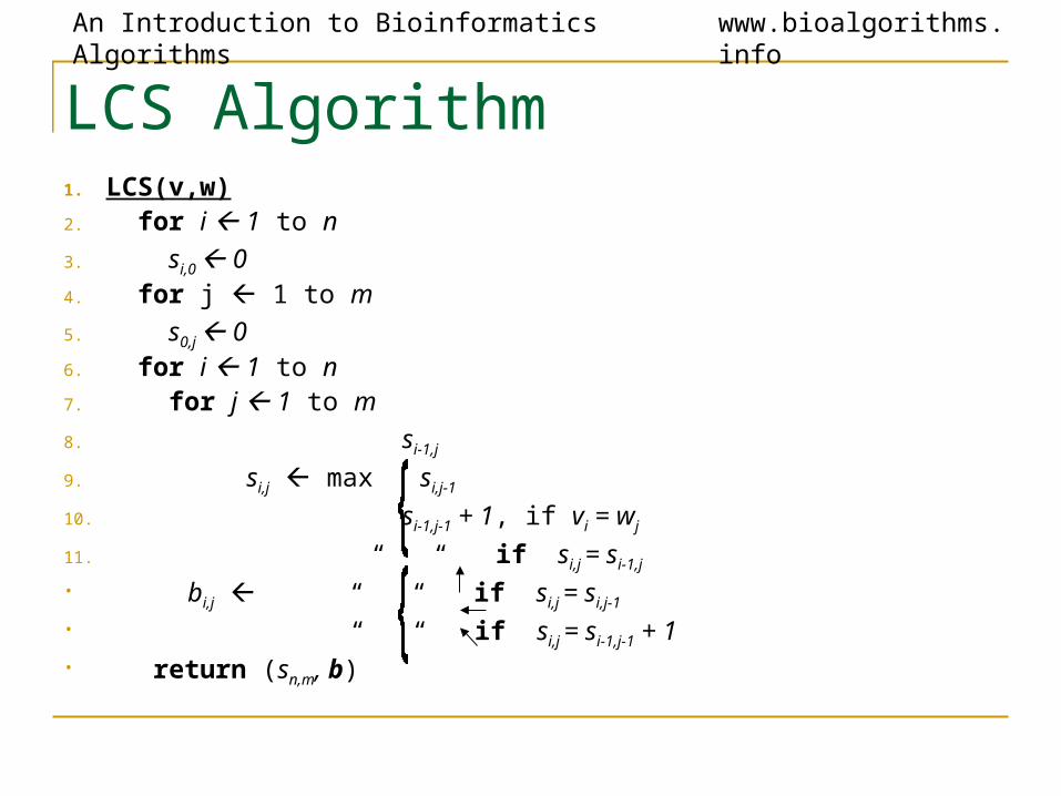
LCS Algorithm1. LCS(v,w)2. for i 1 to n3. si,0 04. for j 1 to m5. s0,j 06. for i 1 to n7. for j 1 to m8. si-1,j
9. si,j max si,j-1
10. si-1,j-1 + 1, if vi = wj
11. “ “ if si,j = si-1,j
• bi,j “ “ if si,j = si,j-1
• “ “ if si,j = si-1,j-1 + 1
• return (sn,m, b)
An Introduction to Bioinformatics Algorithms www.bioalgorithms.info
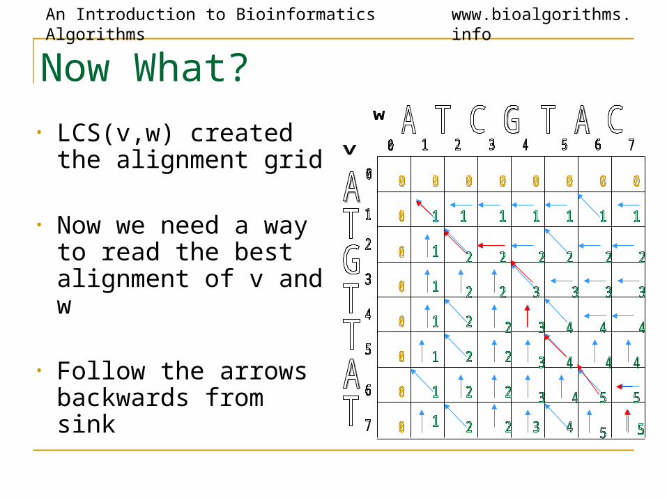
Now What?
• LCS(v,w) created the alignment grid
• Now we need a way to read the best alignment of v and w
• Follow the arrows backwards from sink
An Introduction to Bioinformatics Algorithms www.bioalgorithms.info
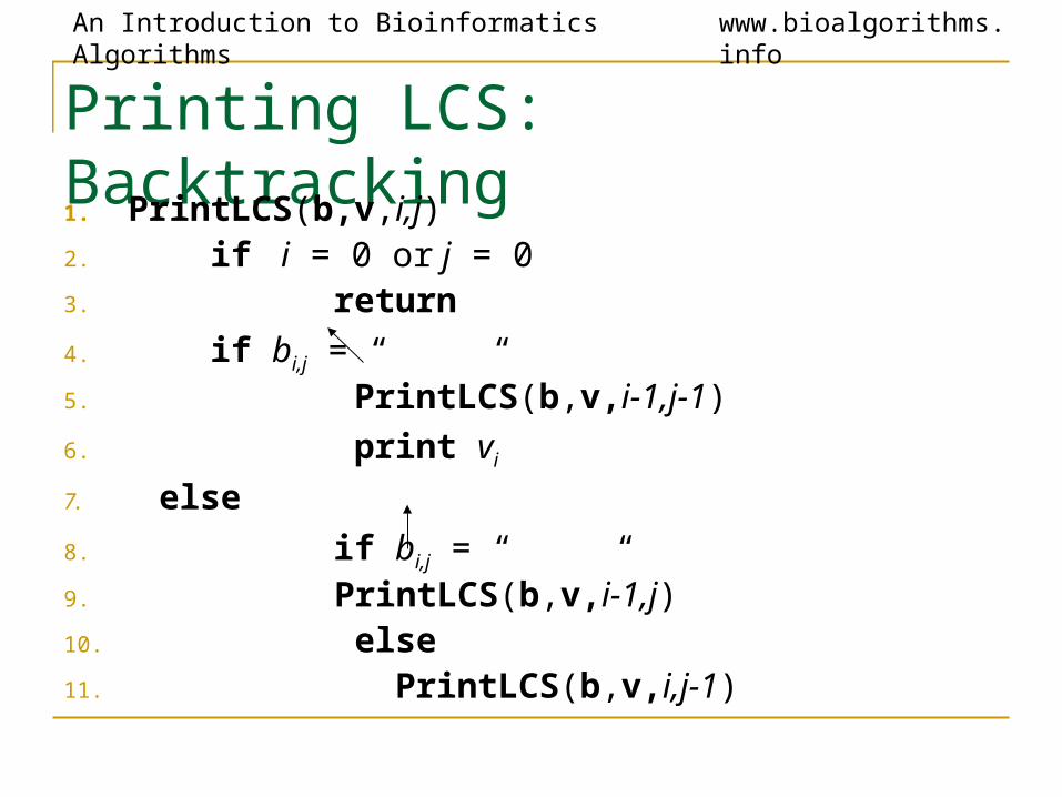
Printing LCS: Backtracking
1. PrintLCS(b,v,i,j)2. if i = 0 or j = 03. return4. if bi,j = “ “5. PrintLCS(b,v,i-1,j-1)6. print vi
7. else
8. if bi,j = “ “9. PrintLCS(b,v,i-1,j)10. else11. PrintLCS(b,v,i,j-1)
An Introduction to Bioinformatics Algorithms www.bioalgorithms.info
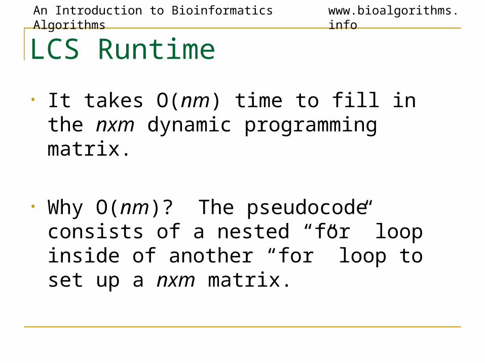
LCS Runtime
• It takes O(nm) time to fill in the nxm dynamic programming matrix.
• Why O(nm)? The pseudocode consists of a nested “for” loop inside of another “for” loop to set up a nxm matrix.