working paper series - european central bank · sovereign debt ratings? 1 by antónio afonso 2,...

ISSN 1561081-0

9 7 7 1 5 6 1 0 8 1 0 0 5

WORKING PAPER SER IESNO 711 / JANUARY 2007

WHAT “HIDES” BEHIND SOVEREIGN DEBT RATINGS?

by António Afonso, Pedro Gomes and Philipp Rother

In 2007 all ECB publications

feature a motif taken from the €20 banknote.

WORK ING PAPER SER IE SNO 711 / JANUARY 2007

This paper can be downloaded without charge from http://www.ecb.int or from the Social Science Research Network

electronic library at http://ssrn.com/abstract_id=954705.

WHAT “HIDES” BEHIND SOVEREIGN DEBT RATINGS? 1

by António Afonso 2, Pedro Gomes 3 and Philipp Rother 4

1 We are grateful to Fitch Ratings, Moody’s, and Standard & Poor’s for providing us historical sovereign rating data, to Renate Dreiskena for help with the data, to Vassilis Hajivassiliou and Philip Vermeulen for helpful clarifications, to Moritz Kraemer, participants at an

ECB seminar, and an anonymous referee for useful comments. The opinions expressed herein are those of the authors and do not necessarily reflect those of the the ECB or the Eurosystem.

2 European Central Bank, Directorate General Economics, Kaiserstrasse 29, 60311 Frankfurt am Main, Germany; e-mail: [email protected]. ISEG/UTL - Technical University of Lisbon, Department of Economics; UECE – Research Unit on

Complexity and Economics, R. Miguel Lupi 20, 1249-078 Lisbon, Portugal. UECE is supported by FCT (Fundação para a Ciência e a Tecnologia, Portugal); e-mail: [email protected].

3 London School of Economics & Political Science; STICERD – Suntory and Toyota International Centres for Economics and Related Disciplines, Houghton Street, London WC2A 2AE, United Kingdom; e-mail: [email protected]. CIEF – Centre for Research on

Financial Economics, R. Miguel Lupi 20, 1249-078 Lisbon, Portugal. The author would like to thank the Fiscal Policies Division of the ECB for its hospitality and aknowledge financial support of FCT.

4 European Central Bank, Directorate General Economics, Kaiserstrasse 29, 60311 Frankfurt am Main, Germany; e-mail: [email protected].

© European Central Bank, 2007

AddressKaiserstrasse 2960311 Frankfurt am Main, Germany

Postal addressPostfach 16 03 1960066 Frankfurt am Main, Germany

Telephone +49 69 1344 0

Internethttp://www.ecb.int

Fax +49 69 1344 6000

Telex411 144 ecb d

All rights reserved.

Any reproduction, publication and reprint in the form of a different publication, whether printed or produced electronically, in whole or in part, is permitted only with the explicit written authorisation of the ECB or the author(s).

The views expressed in this paper do not necessarily reflect those of the European Central Bank.

The statement of purpose for the ECB Working Paper Series is available from the ECB website, http://www.ecb.int.

ISSN 1561-0810 (print)ISSN 1725-2806 (online)

3ECB

Working Paper Series No 711January 2007

CONTENTS

Abstract 4Non-technical summary 51. Introduction 72. Rating systems and literature 8 2.1. Overview of rating systems 8 2.2. Literature review 93. Methodology 11 3.1. Explanatory variables 11 3.2. Linear regression framework 13 3.3. Ordered response framework 154. Empirical analysis 16 4.1. Data 16 4.2. Linear panel results 18 4.2.1. Full sample 18 4.2.2. Differentiation across sub-periods 20 4.2.3. Differentiation across ratings levels 21 4.3. Ordered probit results 23 4.4. Prediction analysis 24 4.5. Examples of specif ic country analysis 275 Conclusion 29References 32Tables and f igures 34Appendix 1 Data sources 59Appendix 2 Countries and years in most extensive rating sample 60Appendix 3 A logistic transformation 61European Central Bank Working Paper Series 64

Abstract

In this paper we study the determinants of sovereign debt credit ratings using rating notations from the three main international rating agencies, for the period 1995-2005. We employ panel estimation and random effects ordered probit approaches to assess the explanatory power of several macroeconomic and public governance variables. Our results point to a good performance of the estimated models, across agencies and across the time dimension, as well as a good overall prediction power. Relevant explanatory variables for a country's credit rating are: GDP per capita, GDP growth, government debt, government effectiveness indicators, external debt, external reserves, and default history. JEL: C23; C25; E44; F30; F34; G15; H63 Keywords: credit ratings; sovereign debt; rating agencies; panel data; random effects ordered probit

4ECB Working Paper Series No 711January 2007

Non-technical summary

Sovereign credit ratings are a condensed assessment of a government’s ability and

willingness to repay its public debt both in principal and in interests on time. In this,

they are forward-looking qualitative measures of the probability of default put forward

by rating agencies. This paper studies the determinants of sovereign debt credit ratings

of the three main international rating agencies: Standard and Poor’s, Moody’s and Fitch

Ratings. We build an extensive ratings database, with sovereign foreign currency

ratings, attributed by the three agencies, as well as the credit rating outlook, for a panel

of 130 countries from 1970 to 2005.

In the first part of the paper we explain the main econometric approaches to the study of

the determinants of credit ratings focussing on specification of the functional form and

the estimation methodology. There are two major strands of empirical work in the

literature: on the one hand, OLS analysis on a numerical representation of the ratings,

which allows for a straightforward generalization to panel data by doing fixed or

random effects estimation; on the other hand, ordered response models. We discuss in

some detail the main advantages and caveat of the several approaches and suggest an

original specification and a more robust estimation procedure. Our specification allows

for an important distinction between short and long-run impact of the explanatory

variables on the credit rating.

In terms of the regressors, we divide them in four main blocks: macroeconomic

performance (per capita GDP, unemployment rate, inflation rate, real GDP growth),

government performance block (government debt, fiscal balance and government

effectiveness), external balance (external debt, foreign reserves and current account

balance) and other explanatory variables (default history, European Union and regional

dummies).

The main finding is that GDP per capita, real GDP growth, government debt,

government effectiveness, external debt and external reserves, sovereign default

indicator as well as being a member of European Union, are the most important

determinants of the sovereign debt ratings. We find that the government related

variables have a stronger effect than found in existing literature.

5ECB


The large sample allows for a sub-period analysis and for a differentiated analysis of

high and low ratings. While the results are roughly stable across agencies, time periods

and ratings levels, some additional interesting results emerge. For instance, for the low

rating levels, external debt and external reserves are more relevant. On the other hand,

for the early sub-period, 1996-2000, the current account balance was more important,

while external reserves were possibly somewhat more important in the later period,

2001-2005 (for Moody’s and S&P). Moreover, after the Asian crisis, it seems there was

a decline in the relevance of the current account variable in the specifications for

Moody’s and S&P.

In the last part of the paper we analyse some specific country cases. We find that, for

instance, Spain’s rating upgrades since 1998 were mainly due to its good

macroeconomic performance, while Portugal’s deterioration of its creditworthiness

during the same period can be mainly attributed to poor government performance.

Additionally new European Union member countries benefited not only from their good

macroeconomic performance, but also from a credibility effect of joining the European

Union.


1. Introduction

Sovereign credit ratings are a condensed assessment of a government’s ability and

willingness to repay its public debt both in principal and in interests on time. In this,

they are forward-looking qualitative measures of the probability of default put forward

by rating agencies. Naturally, one should try to understand the determinants of credit

ratings, given their relevance for international financial markets, economic agents and

governments. Indeed, sovereign credit ratings are important in three ways. First,

sovereign ratings are a key determinant of the interest rates a country faces in the

international financial market and therefore of its borrowing costs. Second, the

sovereign rating may have a constraining impact on the ratings assigned to domestic

banks or companies. Third, some institutional investors have lower bounds for the risk

they can assume in their investments and they will choose their bond portfolio

composition taking into account the credit risk perceived via the rating notations. For

instance, the European Central Bank when conducting open market operations can only

take as collateral bonds that have at least a single A attributed by at least one of the

major rating agencies.

In this paper we perform an empirical analysis of foreign currency sovereign debt

ratings, using rating data from the three main international rating agencies: Fitch

Ratings, Moody’s, and Standard & Poor’s. We have compiled a comprehensive data set

on sovereign debt ratings, macroeconomic data, and qualitative variables for a wide

range of countries starting in 1990. Regarding the empirical modelling strategy, we

follow the two main strands in the literature. We make use of linear regression methods

on a linear transformation of the ratings and we also estimate our specifications under

an ordered probit response framework.

Our main contribution to the existing literature is the innovation of the estimation

method used and the functional form specification, and the large dataset employed.

Under the linear framework, we argue that random effects estimation will be inadequate

due to the correlation between the country specific error and the regressors, but also that

its alternative, fixed effects estimation will not be very informative. We salvage the

random effects approach by means of modelling the country specific error, which in

practical terms implies adding time-averages of the explanatory variables as additional

7ECB


time-invariant regressors. This setting will allow us to make the constructive distinction

between immediate and long-run effects of a variable on the sovereign rating.

Moreover, we also use a limited dependent variable framework by estimating the

augmented-model using ordered probit and random effects ordered probit specifications.

The latter is the best procedure for panel data as it considers the existence of an

additional normally distributed cross-section error. This approach allows both to

determine the cut-off points throughout the rating scale as well as to test whether a

linear quantitative transformation of the ratings is actually more appropriate than a

possible non-linear transformation. Furthermore, we perform robustness check by

allowing for a sub-period analysis and for a differentiated high and low rating analysis.

We find that in particular six core variables have a consistent impact on sovereign

ratings. These are the level of GDP per capita, real GDP growth, the public debt level

and government effectiveness, as well as the level of external debt and external

reserves. A dummy reflecting past sovereign defaults is also found significant as well

as, in some cases, the fiscal balance and a dummy for European Union countries. It is

noteworthy that fiscal variables turn out to be more important than found in the previous

literature.

The paper is organised as follows. In Section Two we give an overview of the rating

systems and review the relevant related literature. Section Three explains our

methodological choices, specifically regarding the econometric approaches employed.

In Section Four we describe the dataset and report on the empirical analysis, notably in

terms of the estimation and prediction results. Section Five summarises the paper’s

main findings.

2. Rating systems and literature

2.1. Overview of rating systems

We use sovereign credit ratings by the three main international rating agencies,

Moody’s, Standard & Poor’s (S&P) and Fitch Ratings. Although these agencies do not

use the same qualitative codes, in general, there is a correspondence between each

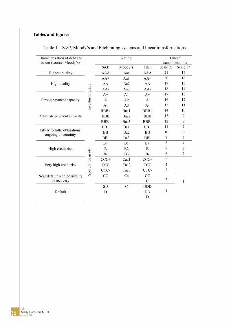
agency rating level as shown in Table 1. S&P and Fitch use a similar qualitative letter


rating in descending order form AAA to CCC-, while Moody’s system goes from Aaa

to Caa3.

[Insert Table 1 here]

2.2. Literature review

Sovereign ratings are assessments of the relative likelihood of default. The rating

agencies assess the risk of default by analysing a wide range of elements from solvency

factors that affect the capacity to repay the debt, but also socio-political factors that

might affect the willingness to pay of the borrower. For example, S&P determines the

rating by evaluating the country’s performance in each of the following areas: political

risk, income and economic structure, economic growth and prospects, fiscal flexibility,

general government debt burden, off-shore and contingent liabilities, monetary

flexibility, external liquidity, public-sector external debt burden and private sector

external debt burden.

Given that the rating materializes out of the analysis of a vast amount of data, it would

be useful to find a reduced set of variables capable of explaining a country’s rating. A

first study on the determinants of sovereign ratings by Cantor and Packer (1996)

concluded that the ratings can be largely explained by a small set of variables namely:

per capita income, GDP growth, inflation, external debt, level of economic

development, and default history. Further studies incorporated more variables.

Macroeconomic performance variables like the unemployment rate or the investment-

to-GDP ratio. In papers focussing on the study of currency crises several external

indicators such as foreign reserves, current account balance, exports or terms of trade

seem to play an important role. Moreover, indicators of how the government conducts

its fiscal policy, budget balance and government debt can also be relevant, as well as

variables that assess political risk, like corruption or social indexes. Table 2 summarises

some of the relevant related studies and findings.


9ECB


Regarding the econometric approach, there are two major strands in the literature. The

first uses linear regression methods on a numerical representation of the ratings. The

early study by Cantor and Packer (1996), applies OLS regressions to a linear

representation of the ratings, on a cross section of 45 countries. This methodology was

also pursued by Afonso (2003), Alexe et al. (2003) and Butler and Fauver (2006). Using

OLS analysis on a numerical representation of the ratings is quite simple and allows for

a straightforward generalization to panel data by doing fixed or random effects

estimation (Monfort and Mulder, 2000; Eliasson, 2002 and Canuto et al., 2004).

Although estimating the determinants of ratings using these approaches has in general a

good fit and a good predictive power it faces some critiques. As ratings are a qualitative

ordinal measure, using traditional estimation techniques on a linear representation of the

ratings is not the most adequate framework of estimation. First, it implies the

assumption that the difference between two rating categories is equal for any two

adjacent categories, which would need to be tested. Furthermore, even if this

assumption was true, because of the presence of elements in the top and bottom

category, the estimates are biased, even in big samples. Nevertheless, Eliasson (2002)

argues that given the existence of many categories one can treat the rating variable as

continuous and to overcome the criticism of the assumption of an even distance between

steps, it is possible to use different quantitative transformations. For instance, Reisen

and Maltzan (1999) apply a logistic transformation of the ratings and Afonso (2003)

applies both a logistic and an exponential transformation of the ratings. In that case, the

differences between categories are not constant, but are still imposed a priori.

The other strand of the literature uses ordered response models. Because the ratings are

a qualitative ordinal measure, the established wisdom advises the use of ordered probit

estimation. This method will itself determine the size of the differences between each

category. For example, this procedure was used by Hu et al. (2002), Bissoondoyal-

Bheenick (2005) and Bissoondoyal-Bheenick et al. (2005). Although this should be

considered the preferred estimation procedure it is not entirely satisfying. The crucial

point is that the ordered probit asymptotic properties do not generalise for a small

sample, so if we estimate the determinants of the ratings using a cross-section of

countries, we would have too few observations. It is therefore imperative to try to

maximize the number of observation by using panel data, but when doing so, one has to


be careful. Indeed, the generalization of ordered probit to panel data is not completely

straightforward, due to the existence of a country specific effect. Furthermore, within

this framework, the need to have many observations makes it harder to perform

robustness analysis by, for instance, partitioning the sample. In Section Three we will

address these questions when explaining our modelling strategy.

3. Methodology

Using a linear scale we grouped the ratings in 17 categories, by putting together in the

same bucket the few observations below B-. Indeed, if we used a specific number for

each existing rating notch, for instance 21 categories, it might be hard to efficiently

estimate the threshold points between CCC+ and CCC, CCC and CCC- and so on, given

that the bottom rating categories have very few observations. Table 1 above also shows

the relation established between the qualitative and the possible linear scales. Moreover,

and as we will see latter in the paper, a linear transformation is quite adherent to the

data. Nevertheless, we also report in Appendix 3 estimation results using a logistic

transformation.

3.1. Explanatory variables

Building on the evidence provided by the existing literature, we identify a set of main

macroeconomic and qualitative variables that may determine sovereign ratings.

GDP per capita – positive impact on rating: more developed economies are expected to

have more stable institutions to prevent government over-borrowing and to be less

vulnerable to exogenous shocks.

Real GDP growth – positive impact: higher real growth strengthens the government’s

ability to repay outstanding obligations.

Inflation – uncertain impact: on the one hand, it reduces the real stock of outstanding

government debt in domestic currency, leaving overall more resources for the coverage

of foreign debt obligations. On the other hand, it is symptomatic of problems at the

macroeconomic policy level, especially if caused by monetary financing of deficits.

11ECB


Unemployment – negative impact: a country with lower unemployment tends to have

more flexible labour markets making it less vulnerable to changes in the economic

environment. In addition, lower unemployment reduces the fiscal burden of

unemployment and social benefits while broadening the base for labour taxation.

Government debt – negative impact: a higher stock of outstanding government debt

implies a higher interest burden and should correspond to a higher risk of default.

Fiscal balance – positive impact: large fiscal deficits absorb domestic savings and also

suggest macroeconomic disequilibria, negatively affecting the rating level. Persistent

deficits may signal problems with the institutional environment for policy makers.

Government effectiveness – positive impact: high quality of public service delivery and

competence of bureaucracy should impinge positively of the ability to service debt

obligations. (We initially used all six World Bank Governance Indicators: voice and

accountability, political stability, regulatory quality, rule of law, control of corruption

and government effectiveness, but only this last one turned up as significant).

External debt – negative impact: the higher the overall economy’s external

indebtedness, the higher becomes the risk for additional fiscal burdens, either directly

due to a sell-off of foreign government debt or indirectly due to the need to support

over-indebted domestic borrowers.

Foreign reserves – positive impact: higher (official) foreign reserves should shield the

government from having to default on its foreign currency obligations.

Current account balance – uncertain impact: a higher current account deficit could

signal an economy’s tendency to over-consume, undermining long-term sustainability.

Alternatively, it could reflect rapid accumulation of fixed investment, which should lead

to higher growth and improved sustainability over the medium term.

Default history – negative impact: past sovereign defaults may indicate a great

acceptance of reducing the outstanding debt burden via a default. The effect is modelled


by a dummy variable indicating the past occurrence of a default and by a variable

measuring the number of years since the last default. This variable measures the

recovery of credibility after a default and can be expected to influence positively the

rating score.

3.2. Linear regression framework

A possible starting point for our linear panel model would follow Monfort and Mulder

(2000), Eliasson (2002) or Canuto, Santos and Porto (2004), generalizing a cross section

specification to panel data,

it it i i itR X Z aβ λ µ= + + + , (1)

where we have: R – quantitative variable, obtained by a linear or by a non-linear

transformation; Xit is a vector containing time varying variables that includes the time-

varying explanatory variables described above and Zi is a vector of time invariant

variables that include regional dummies.

In (1) the index i (i=1,…,N) denotes the country, the index t (t=1,…,T) indicates the

period and ai stands for the individual effects for each country i (that can either be

modelled as a error term or as N dummies to be estimated). Additionally, it is assumed

that the disturbances µit are independent across countries and across time.

There are three ways to estimate this equation: pooled OLS, fixed effects or random

effects estimation. In normal conditions all estimators are consistent and the ranking of

the three methods in terms of efficiency is clear: a random effects approach is preferable

to the fixed effects, which is preferable to pooled OLS. The question one should ask is

whether the normal conditions are fulfilled. What we mean by normal conditions is

whether or not the country specific error is uncorrelated with the regressors E(ai| Xit,

Zi)=0. If this is the case one should opt for the random effects estimation, while if this

condition does not hold, both the pooled OLS and the random effects estimation give

inconsistent estimates and fixed effects estimation is preferable.

13ECB


In our case, it seems more natural that the country specific effect is correlated with the

regressors.1 Given this scenario one should be tempted to say that the “fixed effects

estimation” is the best strategy, but that has a problem. Because there is not much

variation of a countries rating over time, the country dummies included in the regression

will capture the country’s average rating, while all the other variables will only capture

movements in the ratings across time. This means that, although statistically correct, a

regression by fixed effects would be seriously striped of meaning.

There are two ways of rescuing a random effects approach under correlation between

the country specific error and the regressors. One is to do the Hausman-Taylor IV

estimation but for that we would have to come up with possible instruments that are not

correlated with ai, which does not seem an easy task. In this paper we will opt for a

different approach that consists on modelling the error term ai. This approach, described

in Wooldridge (2002), is usually applied when estimating non-linear models, as IV

estimation proves to be a Herculean task but, as we shall see, the application to our case

is quite successful. The idea is to give an explicit expression for the correlation between

the error and the regressors, stating that the expected value of the country specific error

is a linear combination of time-averages of the regressors iX . This follows Hajivassiliou

and Ioannides (2006) and Hajivassiliou (2006).

( | , ) ii it iE a X Z Xη= . (2)

If we modify our initial equation (1), with ti ia Xη ε= + we get

iXit it i i itR X Zβ λ η ε µ= + + + + , (3)

where iε is an error term by definition uncorrelated with the regressors. In practical

terms, we eliminate the problem by including a time-average of the explanatory

variables as additional time-invariant regressors. We can rewrite (3) as:

1 This idea can easily be checked by doing some exploratory regressors. We estimated equation (1) using random effects and performed the Hausman test; the Qui-Square statistisc was in fact very high, and the null hypothesis of no correlation was rejected with p-values of 0.000.


( X ) ( )Xi iit it i i itR X Zβ η β λ ε µ= − + + + + + . (4)

This expression is quite intuitive.δ η β= + can be interpreted as a long-term effect (e. g.

if a country has a permanent high inflation what is the respective effect on the rating),

while β is a short-term effect (e. g. if a country manages to reduce inflation this year by

one point what would be the effect in the rating). This intuitive distinction is useful for

policy purposes as it can tell what a country can do to improve its rating in the short to

medium-term. We will estimate equation (4) by random effects, but we also estimate the

OLS and fixed effects versions. The way we modelled the error term can be considered

successful if the coefficients of iX are significant and if the Hausman test indicates no

correlation between the regressors and the new error term.

3.3. Ordered response framework

Alternatively we estimate the determinants of sovereign debt ratings in a limited

dependent variable framework. As we mentioned before, the ordered probit is a natural

approach for this type of problem, because the rating is a discrete variable and reflects

an order in terms of probability of default. The setting is the following. Each rating

agency makes a continuous evaluation of a country’s credit-worthiness, embodied in an

unobserved latent variable R*. This latent variable has a linear form and depends on the

same set of variables as before,

* ( X ) Xi iit it i i itR X Zβ δ λ ε µ= − + + + + . (5)

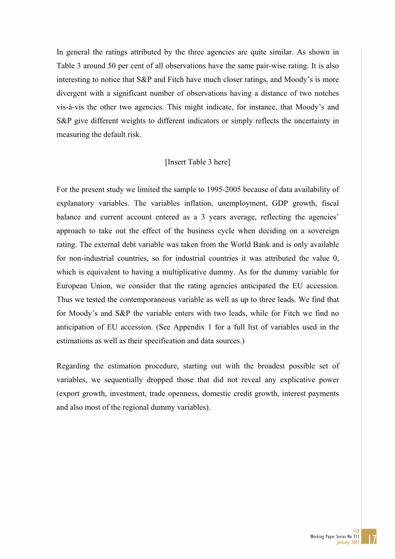
Because there is a limited number of rating categories, the rating agencies will have

several cut-off points that draw up the boundaries of each rating category. The final

rating will then be given by

*16

*16 15

*15 14

*1

( ) ( 1)

( 2)

( 1)

it

it

it it

it

AAA Aaa if R cAA Aa if c R c

R AA Aa if c R c

CCC Caa if c R

⎧ >⎪ + > >⎪⎪= > >⎨⎪⎪⎪< + >⎩

M. (6)

15ECB


The parameters of equation (5) and (6), notably β, δ, λ and the cut-off points c1 to c16 are

estimated using maximum likelihood. Since we are working in a panel data setting, the

generalization of ordered probit is not straightforward, because instead of having one

error term, we now have two. Wooldridge (2002) describes two approaches to estimate

this model. One “quick and dirty” possibility is to assume we only have one error term

that is serially correlated within countries. Under that assumption one can do the normal

ordered probit estimation but a robust variance-covariance matrix estimator is needed to

account for the serial correlation. The second possibility is the random effects ordered

probit model, which considers both errors εi and µit to be normally distributed, and the

maximization of the log-likelihood is done accordingly. This second approach should be

considered the best one, but it has as a drawback the quite cumbersome calculations

involved. In STATA this procedure was created by Rabe-Hesketh et al. (2000) and

substantially improved by Frechette (2001a, 2001b), and we will use such procedures in

our calculations.

4. Empirical analysis

4.1. Data

We build a ratings database with sovereign foreign currency rating attributed by the

three above-mentioned main rating agencies. For the rating notations we covered a

period from 1970 to 2005. The rating of a particular year is the rating that was attributed

at 31st of December of that year. In 2005 there are 130 countries with a rating, though

only 78 have a rating attributed by all three agencies (see Appendix 2 for rating

coverage description).2

In Figure 1 we can see the evolution of the number of countries rated by each agency

and it is possible to notice a significant increase in mid 1990’s of the number of

countries with rating, especially from S&P and Moody’s.

[Insert Figure 1 here]

2 The full historical rating dataset that we compiled, including foreign and local currency ratings as well as credit rating outlooks, is available from the authors on request.


In general the ratings attributed by the three agencies are quite similar. As shown in

Table 3 around 50 per cent of all observations have the same pair-wise rating. It is also

interesting to notice that S&P and Fitch have much closer ratings, and Moody’s is more

divergent with a significant number of observations having a distance of two notches

vis-à-vis the other two agencies. This might indicate, for instance, that Moody’s and

S&P give different weights to different indicators or simply reflects the uncertainty in

measuring the default risk.


For the present study we limited the sample to 1995-2005 because of data availability of

explanatory variables. The variables inflation, unemployment, GDP growth, fiscal

balance and current account entered as a 3 years average, reflecting the agencies’

approach to take out the effect of the business cycle when deciding on a sovereign

rating. The external debt variable was taken from the World Bank and is only available

for non-industrial countries, so for industrial countries it was attributed the value 0,

which is equivalent to having a multiplicative dummy. As for the dummy variable for

European Union, we consider that the rating agencies anticipated the EU accession.

Thus we tested the contemporaneous variable as well as up to three leads. We find that

for Moody’s and S&P the variable enters with two leads, while for Fitch we find no

anticipation of EU accession. (See Appendix 1 for a full list of variables used in the

estimations as well as their specification and data sources.) Regarding the estimation procedure, starting out with the broadest possible set of

variables, we sequentially dropped those that did not reveal any explicative power

(export growth, investment, trade openness, domestic credit growth, interest payments

and also most of the regional dummy variables).

17ECB


4.2. Linear panel results

4.2.1. Full sample

The results generated by the panel regressions point to broadly similar regression

models across the three rating agencies (see Tables 4, 5 and 6). In view of the analytical

considerations above the discussion will focus on the random effects estimations. This

is supported by the Hausmann tests reported at the end of each table pointing to the

acceptability of the random effects approach. Nevertheless, we also report the pooled

OLS and the fixed effects results for completeness and comparison purposes.

[Insert Tables 4, 5 and 6 here]

We report the results of two models for each of the rating agencies, the unrestricted and

the restricted model. While the unrestricted model incorporates all variables discussed

above, the restricted model contains only the variables which were found to have a

statistically significant impact. Although the sequence of excluding individual variables

in moving from the unrestricted to the restricted regression can have an impact on the

final specfication, the restricted models presented in the tables are quite robust to

alternative exclusion procedures. As can be seen from the statistics reported at the end

of each table, the explanatory power of the models is very high with R-square values

around 95 per cent and it remains almost constant moving from the unrestricted to the

restricted versions, while the number of observations increases marginally. In addition,

the variables found to be significant in the unrestricted model generally remain

significant with the same sign in the restricted version.

The restricted models reveal a homogenous set of explanatory variables across agencies.

On the real side, GDP per capita and GDP growth rates turn out significant for all three

companies. In the fiscal area, this applies to the government debt ratio as a difference

from the average and to the government effectiveness indicator. On the external side,

the average external debt ratio and the average level of reserves are found to be

significant across agencies. Default, EU and industrial country dummies are also

significant for all agencies. Moreover, the size of the coefficients is of the same order of

magnitude and they have the expected signs. In particular, the level and growth rate of


real income drive up the rating, government and external debt have a negative impact

and government effectiveness and higher external reserves have a positive impact.

Beyond this set of core variables, the agencies appear to employ a limited number of

additional variables. For Fitch the analysis finds the smallest set of additional variables,

comprising government effectiveness as a deviation from the average and foreign

currency reserves also as the short-run deviation. By contrast, the analysis finds more

significant explanatory variables for Moody’s and Standard and Poor’s, with a large

degree of homogeneity between these two agencies. In particular, on the real side

inflation is found to have a significantly negative impact. In the fiscal area, the average

debt level exerts an additional negative impact on the ratings level, whereas the fiscal

balance has a strong positive impact. With regard to the external sector, the current

account balance has a negative impact.

The findings regarding the current account effect may appear surprising as it suggests

that countries with high current account surpluses would tend to be rated lower than

otherwise equal countries without such surpluses. However, this result is quite recurrent

in the literature (Monfort and Mulder, 2000 or Eliasson, 2002). A possible explanation

is that a current account deficit could in fact serve as an indicator for the willingness of

foreigners to cover the current account gap through loans and foreign investment. In this

situation, a higher current account deficit would be associated with either higher credit-

worthiness or good economic prospects of the economy and consequently a higher

sovereign rating.

Finally, the impact of the unemployment variables appears not entirely clear cut. While

the average level of unemployment is found to have a significant negative impact on the

rating by Moody’s, the short-run deviation from the average enters positively and

significantly in the S&P model. Structural reforms that raise unemployment in the short

run but improve fiscal sustainability in the long run could provide an explanation for

this latter finding, but further research would be necessary to validate this hypothesis.

One can also assess how successfull and important our specification is. First, most of

the time averages of the explanatory variables are significant, which proves that if we

19ECB


did not include them we would be mispecifying the model.3 Second, the models pass the

Hausman test, which sugested that the problem was entirely corrected. Furthermore, if

we look at the fixed effects estimation we can see how poor it is. Notice the estimated

constant and its significance. In general the constant captures the middle rating, while

the estimated country dummies (ommited here), which vary from -7 to 7 notches,

capture each country’s average rating. All the other variables only capture small

movements from the rating in relation to its average4.

4.2.2. Differentiation across sub-periods

The separation of the overall sample into two sub-periods allows to assess broadly the

robustness of the empirical models and provides additional insight into possible changes

in the rating determinants. In particular, cutting the sample period in 2000 could reveal

any changes in the sovereign ratings methodology in response to the Asian crisis which

was perceived by market participants as revealing previously underestimated risks to

sovereign sustainability. Additionally, this also divides the full sample in two rather

similar sized sub-samples.

The models for the sub-periods are generally in line with those for the full estimation

period, although the significance levels of the individual coefficients are reduced (see

Tables 7–9). The lower significance levels reflect the reduction in the respective sample

sizes in half, which makes the coefficient estimates less certain. Taking this into

account, signs and orders of magnitude of the coefficient estimates from the full-period

models are mostly confirmed for the sub-periods. In particular, the core variables

identified above enter the models for the sub-periods with the correct sign and generally

significantly with a comparable order of magnitude.


Regarding the possible impact of the Asian crisis on ratings approaches, the stability of

the ratings models suggests that there was no fundamental change in methodologies. A

3 This is in fact the cause why without including time-averages the models would not pass the Hausman test. 4 We also estimated the model with the average rating of the three agencies, and also pooling the data for the three agencies, but the results where quite similar.


change that may point to some adaptation of ratings methods in response to the Asian

events is the decline in importance of the current account variable for Moody’s and

S&P, both with regard to the value of the estimated coefficient as well as its

significance level. The change may suggest that the function of the current account as

an indicator for foreigners’ willingness to cover the current account gap has declined.

Finally, for Moody’s the increase in value and significance of the coefficient on external

reserves may point to a higher importance attached to this variable after the Asian crisis.

Taken together with the reduced importance of the current account, this could suggest a

move towards a broader view on foreign financial relationships, which includes capital

flows in addition to the current account movements.

Looking at the individual agencies, for Fitch coefficient values remain remarkably

stable over the sub-periods. An exception is the negative (though insignificant) value for

GDP growth in the early sub-sample. For S&P, sign reversals between sub-periods

occur for the explanatory variables unemployment, government effectiveness and

external debt, but there are no significant coefficient estimates with opposing signs. For

Moody’s, the models point to a sign reversal for the insignificant estimate of the

coefficient on inflation.

4.2.3. Differentiation across ratings levels

As a further test of the robustness of the results derived above, the sample was split into

two groups according to the ratings level: regressions were run separately for high-rated

countries with grades BBB+ and below and those above this grade. The choice of the

threshold reflects practical considerations. While market participants generally divide

bond issuers into investment-grade and non-investment grade at the threshold of BBB-,

this threshold would result in a relatively small number of observations for low ratings

making inference problematic. From the estimation of the ratigns above BBB+, we

removed the variable external debt because there were too few observations of non-

industrial countries.

The results for the separate regressions according to ratings levels confirm the overall

results from the full sample (see Tables 10–12). Looking at the random effects

estimation for each agency, the variables that were found to be significant across

21ECB


agencies in the full sample also show up consistently with the correct sign in the

individual regression models for high and low ratings. Most of the coefficients are

statistically significant. Notably, the importance of average external reserves appears to

rise for low ratings in the models for Fitch and S&P. In the cases of statistical

significance external reserves always have a positive impact on the ratings.


The explanatory power of the individual regressions is somewhat lower than that found

for the full sample as well as for the sub-periods. This reflects the fact that splitting the

sample in this way reduces the number of rating categories for each estimation, so that,

with a discrete dependent variable, estimated rating errors become relatively larger.

Beyond the core variables, the results for Moody’s and S&P suggest a significant

difference in the importance of inflation for high and low ratings, respectively. For both

agencies the (significant) coefficient on inflation as an average and the deviation from it

is much higher for high ratings than for low ratings. (For Fitch, this finding is supported

by the pooled OLS and the fixed effects estimations, but not for the random effects

specification.) This suggests that for high rated countries inflation has a much more

important impact on the rating. A possible explanation is that for this set of countries

price level stability may be taken as an indicator for sound economic and in particular

monetary policies which support the long-run sustainability of government finances.

Turning to differences across agencies, the results point to a relatively high level of

consistency in the approach to high and low ratings for Fitch and Moody’s. For these

two agencies signs and (mostly) significance levels of coefficient are generally

consistent for high and low ratings. A somewhat higher degree of variation in this

regard can be observed for S&P where the sign of the estimated impact of some

variables switches between high and low ratings, although in most instances the

comparison involves statistically insignificant coefficients. Additionally, one notices

also a higher R-square for low ratings for S&P and Fitch.


4.3. Ordered probit results

In view of the discussion of econometric issues above, ordered probit models should

give additional insight into the determinants of sovereign ratings. In particular, this

method allows to relax the rigid assumption on the shape of the ratings schedule.

Instead it generates estimates of the threshold values between rating notches allowing an

assessment of the shape of the ratings curve. Given the data requirements, the method

was only applied to the full sample, which appears appropriate in view of the overall

robustness of the empirical results to the use of sub-samples.

The results from the ordered probit estimation validate the findings highlighted above

(see Tables 13 and 14, respectively for the ordered probit robust standard errors and the

random effects ordered probit). The core variables identified in the linear regressions

also show up with the correct sign in the ordered probit approach. In addition, the

ordered probit models suggest the significance of somewhat more explanatory variables,

namely inflation and the current account, which were significant only in some

specifications in the linear approach. At the same time, in the area of external variables,

reserves do not show up significantly for Moody’s and Fitch in the restricted

specifications, both for the ordered probit and for the random effects ordered probit.

Finally, for the current account variable, the restricted specification for Moody’s shows

a negative sign for deviations from the long-term average, but a positive sign for the

average, and similar sign switches appear also in some instances for the other agencies.

This result goes some way in reconciling the counter intuitive result of the negative

effect of current account on sovereign ratings, with the conventional wisdom.

[Insert Tables 13 and 14 here]

The estimated threshold coefficients reported in the second part of the tables suggest

that the linear specification assumed for the panel regression above is appropriate. The

plot of the results of the random effects ordered probit (see Figure 2), shows that for all

three agencies the thresholds between rating notches are broadly equally distributed

across the ratings range. In other words, the distance for a country to move e.g. from B–

to B is roughly equal to that for moving from AA to AA+. Nevertheless, the

econometric tests at the bottom of the tables reveal additional insights. For the restricted

23ECB


model of Moody’s, the test does not reject the null hypothesis of equal distances

between thresholds, but the significance level is close to 10 per cent. Indeed the

estimated thresholds point to a relatively large jump between the ratings for BBB– and

BBB. This suggests that countries close to the non-investment grade rating are given a

wider range before they actually cross that threshold. For Fitch, the hypothesis of equal

distances is strongly rejected as the thresholds for higher ratings are further apart than

those of the lower ratings. In this case the kink lies at the A rating.


Finally, for S&P, different distances are found throughout the ratings scale. Looking at

Figure 2, it appears that for lower ratings the relative distance between thresholds of

S&P coincides with that of Moody’s. However, above the investment grade limit, the

distances between thresholds at first decline and then increase, resulting in a slightly

curved ratings schedule that makes the transition to the highest grades most difficult.

4.4. Prediction analysis

Our prediction analysis will focus on two elements: the prediction for the rating of each

individual observation in the sample, as well as the prediction of movements in the

ratings through time.

Prediction with the pooled OLS model was done by rounding the fitted value (which is

continuous) to the closest integer between 1 and 17. For the random effects estimations

we can have two predictions, with or without the country specific effect, εi, and we can

write the corresponding estimated versions of (4) as:

ˆ ˆ ˆˆ ˆ( X ) Xi iit it i iR X Zβ δ λ ε= − + + + , (7a)

ˆ ˆ ˆ( X ) Xi iit it iR X Zβ δ λ= − + +% . (7b)

We can then estimate each country specific effect by taking the time average of the

estimated residual for each country. As a result we can include or exclude this


additional information that comes out of the estimation. In other words, we generate in-

sample and out-of-sample prediction. After the fitted value is computed it is then also

rounded to the closest integer between 1 and 17. The prediction with both ordered probit

and the random effects ordered probit was done by fitting the value of the latent

variable, setting the error term to zero, and then match it up to the cut points do

determine the predicted rating. Table 15 presents an overall summary of the prediction

errors, for the three agencies and for the several methods using the respective restricted

specifications.


The first conclusion is that the random effects model including the estimated country

effect is the method with the best fit. On average for the three agencies, it correctly

predicts 70 per cent of all observations and more than 95 per cent of the predicted

ratings lie within one notch (99 per cent within two notches). This is not surprising, the

country errors capture factors like political risk, geopolitical uncertainty and social

tensions that are likely to systematically affect the ratings, therefore, such term acts like

a correction for these factors.

This additional information cropping up from the random effects estimation with the

country specific effect can be very useful if we want to work with countries that belong

to our sample. But if we want to make out of sample predictions we will not have this

information. In that case, only the random effects estimation excluding the country error

is comparable to the OLS specification, to the ordered probit and to the random effects

ordered probit. We can see that in general both ordered probit and random effects

ordered probit have a better fit than the pooled OLS and random effects for all three

agencies, though not as clearly for Fitch. Overall, the simple ordered probit seems the

best method as far as prediction in levels is concerned as it predicts correctly around 45

per cent of all observations and more then 80 per cent within one notch.

Another interesting aspect to notice is that the OLS and the random effects

specifications are biased downward, while the ordered probit and random effects

ordered probit ones are slightly biased upward. The explanation for this turns out to be

simple if we look at Figures 3 to 5, were we present a map of predicted versus actual

25ECB


rating for every category using the four estimation methods. We can see that both the

OLS and the random effects specifications tend to under predict actual AAA’s (Aaa)

while both ordered probit models and random effects ordered probit tend to over predict

the actual rating in the top categories, attributing many AAA’s (Aaa) to countries with

actual lower rating. In the bottom end of the rating scale the opposite happens, OLS and

random effects have a propensity to overestimate ratings that are bellow CCC+ (Caa1),

on the other hand, both ordered probit prediction errors are quite balanced.

[Insert Figures 3, 4 and 5 here]

Those figures provide some additional insights. For Moody’s, ordered probit performs

well in the bottom ratings while random effects ordered probit is better for top ratings.

Also notice that all four models have difficulty explaining the rating A3. Out of 21

observations the maximum correctly predicted is 2 (with OLS) with a substantial

number of predictions lying outside 1 notch.

For S&P the ordered probit outperforms all other models in the middle and bottom

categories. For Fitch, one should mention that the number of observations used for the

random effects ordered probit is higher than the other models (because of the non-

inclusion of one of the variables), which makes comparison harder. One element we

need to highlight is the fact that there is only one observation in the category A+, which

is the possible cause for the identification of the jump in both limited dependent

variable estimations, mentioned before in section 4.4. For completeness, Figure 6

reports the map of predicted ratings using the random effects estimation including

country specific errors.


Let’s now turn to how the models perform in predicting changes in ratings. Table 16

presents the total number of sample upgrades (downgrades), the predicted number of

upgrades (downgrades) and the number of upgrades (downgrades) that where correctly

predicted by the several models.



Roughly the models correctly predict between one third and one half of both upgrades

and downgrades. In our opinion this is quite satisfactory given that the empirical

approach used here necessarily neglects two sources of information that are known to

enter the decision of the rating agencies. First, in contrast to the backward-looking

models presented above, rating agencies base their decision to a considerable extent on

projected economic developments. Thus, a full empirical model of the agencies’

approach would need to incorporate the agencies’ expectations regarding the relevant

explanatory variables. However, as the agencies generally do not publish their

projections, any such modelling attempt would remain highly tentative. Still, the

observation that many of the actual rating changes are predicted by the models with a

lag of one or two years appears to support the relevance of this point. Second, ratings

agencies also generally make a clear point that they cover qualitative variables in

addition to quantitative data in the ratings process. While the relative importance of the

qualitative and quantitative factors that enter the ratings decision is uncertain (and might

well vary across countries), rating agencies’ public statements indicate that such factors

can play an important role.5 In the models above, by contrast, the only variable

reflecting such considerations is the government effectiveness indicator and it thus

appears likely that in these models the impact of qualitative factors is under-represented.

The most noticeable difference between the models is not the number of corrected

predicted changes but the total number of predicted changes. In fact, the ordered probit

and random effects ordered probit predict significantly more changes than the OLS and

random effects counterparts. For instance, for S&P, while both OLS and random effects

predict around 79 upgrades and 50 downgrades, the ordered probit model predicts 102

upgrades and 64 downgrades.

4.5. Examples of specific country analysis

In terms of the magnitude of the coefficients, the comparison between the ordered probit

and random effects ordered probit is not straightforward because the estimated distances

between the categories are different. But in general, once this is accounted for, by

5 For example, see Rother (2005) for an analysis of the impact of EMU convergence on country ratings in eastern Europe.

27ECB


standardising the coefficients in relation to the average jump, they are both in line with

the linear panel results. An improvement of 2 percentage points in the budget deficit, a

reduction of 5 percentage points in public debt, or a higher GDP growth by 3 percentage

points, all have the same relative impact on the ratings between 0.1 and 0.2 notches. An

increase of 10 per cent in GDP per capita would improve the rating by 0.15 to 0.25

notches. As we mentioned, a reduction of the unemployment only affects the rating if

this reduction is sustainable. If that is the case, a reduction of 4 percentage points

increases the rating by 0.2 to 0.35 notches. The effect of inflation is quite small, a

reduction of 20 percentage points on inflation increases the rating by 0.05 to 0.1

notches. These values are too small to be noteworthy for industrial countries, but if one

does the same calculation with the value estimated for high rated countries a reduction

of 4 percentage points in inflation would increase the rating by 0.15 notches.

Now that we have an idea of the estimated impact of the variables we can do some

specific country analysis. As an example, in Table 17 we show the rating for some

European countries and some emerging markets both in 1998 and 2005. Then, we use

the estimated short-run coefficients of the random effects ordered probit together with

the values for the relevant variables. Afterwards, we divide the overall prediction

change in the rating for each agency into the contributions of the different blocks of

explanatory variables: macroeconomic performance, government and fiscal

performance, external elements and European Union6. The upper and lower bound

presented are computed by adding and subtracting one standard deviation to the point

estimate of the coefficients.


Let’s compare, for instance, Portugal and Spain. In 1998 they both had an AA (Aa2)

rating but in 2005 while Spain had been upgraded to AAA (Aaa) by all agencies,

Portugal had been downgraded by S&P. If we analyse the contributions of the main key

variables we see that, for Portugal the positive contribution of the macroeconomic

performance was overshadowed by the negative government developments. For such

6 As an exception, we used the long-run coefficient of unemployment instead of the short-run coefficient. We are implicitly assuming that all the changes in unemployment between these two years were structural.


government performance contributed the worsening of the budget deficit since 2000, the

upward trend in government debt and the worsening in the World Bank governance

effectiveness indicator. As for Spain, the good macroeconomic performance was the

main cause of the upgrade, specially the reduction of structural unemployment since the

mid nineties and the increase of GDP per capita due to the persistent high growth.

Another example can be seen with the new European Union member states Slovakia,

the Czech Republic, Hungary, Slovenia and Poland, which have in general been

upgraded by the three agencies, in some cases more than two notches. The good

macroeconomic performance, especially in Slovakia and the Czech Republic, plays a

major role, but there was also an important credibility effect of joining the European

Union, mostly visible for Moody’s. It is in fact for Moody’s that we observe the

strongest upgrades. For Poland, the effect of the macro performance might be

undervalued. One of the key elements was the sharp reduction of inflation of more then

12 percentage points, but, as we mentioned before, the effect of inflation for high rated

countries is under assessed in the main estimations. If we consider such information,

one would have an estimated additional impact of almost half a notch.

As a final example for the emerging economies, we report the results for five countries

that have, in general also been upgraded: Brazil, Mexico, Malaysia, Thailand and South

Africa. We should briefly highlight that for Brazil the main positive contribution came

from the external area specially the reduction of external debt and the increase in

foreign reserves. This effect is particular to Fitch. For Malaysia and Thailand the main

contribution came from the macro side, while for Mexico and South Africa the

contributions are more balanced.

5. Conclusion

In this paper we studied the determinants of global sovereign debt ratings using ratings

from the three main international rating agencies, for the period 1995-2005. Overall, our

results point to a good performance of the estimated models, across agencies and across

the time dimension, as well as a good overall prediction power.

29ECB


Regarding the methodological approach, we used both a linear framework and an

ordered probit approach. We modelled the country specific error using a random effects

approach, which in practical terms implied adding time-averages of the explanatory

variables as additional time-invariant regressors. This setting allowed us to distinguish

between immediate and long-run effects of a variable on the sovereign rating level.

Moreover, we also used a limited dependent variable framework by means of an ordered

probit and random effects ordered probit specifications. The latter is the best procedure

for panel data as it considers the existence of an additional normally distributed cross-

section error term. This approach allowed both to determine the cut-off points

throughout the rating scale as well as assessing whether a linear quantitative

transformation of the ratings is actually more appropriate than a possible non-linear

transformation.

Our main findings in the panel random effects framework allowed us to detect a set of

core variables that are relevant for the determination of the ratings: per capita GDP;

GDP real growth rate; government debt; government effectiveness; external debt and

external reserves; sovereign default indicators. Moreover, the importance of fiscal

variables appears stronger than in the previous existing literature.7

The ordered probit analysis confirmed the overall estimation results from the linear

panel regressions. Interestingly, there is some evidence for different approaches of the

agencies with regard to the distance between ratings thresholds. For instance, for

Moody’s the estimated thresholds point to a relatively large jump between the ratings

for BBB– and BBB. This suggests that countries close to the non-investment grade

rating are given a wider range before they actually cross that threshold. For Fitch, the

hypothesis of equal distances is strongly rejected as the thresholds for higher ratings are

further apart than those of the lower ratings. In this case the kink lies at the A rating. On

the other hand, no clear switching pattern emerges for S&P.

The panel sample we used is quite comprehensive, which allowed for a sub-period

analysis and for a differentiated high and low rating analysis. While the results are

7 We performed additional analysis from some different perspectives. For instance, we used the information on credit rating outlooks but no relevant improvement on the fit of the models occurred. In addition, we assessed also whether different exchange rate regimes added information to the rating determination, but that was not the case.


roughly stable across agencies, time periods and ratings levels, some additional

interesting results emerge. For instance, for the low rating levels, external debt and

external reserves are more relevant. On the other hand, for the early sub-period, 1996-

2000, the current account balance was more important, while external reserves were

possibly somewhat more important in the later period, 2001-2005 (for Moody’s and

S&P). Moreover, after the Asian crisis, it seems there was a decline in the relevance of

the current account variable in the specifications for Moody’s and S&P.

Another relevant outcome ot the analysis ist that low ratings levels are more affected by

external debt and external reserves while inflation plays a bigger role for high rating

levels. On the other hand, the specifications for the Fitch ratings seem to be most

consistent over time and ratings categories. There was more variation for S&P and

Moody’s in the middle of the rating scales, which possibly points to a more quantitative

model-based approach for Fitch.

Finally, regarding the prediction analysis, the random effects model including the

estimated country effect turns out to be the method with the best fit. On average for the

three agencies, such specification correctly predicted 70 per cent of all observations and

more than 95 per cent of the predicted ratings lay within one notch. Moreover, the

models also correctly predicted between one third and one half of respectively upgrades

and downgrades. This is quite satisfactory for two reasons: first, the rating agencies also

have a forward looking behaviour that is absent from our models and second, other

qualitative factors not captured in our variables may play an important role.

Looking forward, further studies could investigate how to capture agencies’

expectations in empirical models as well as their views on qualitative variables.

Moreover, in our modelling approach we only use the government effectiveness

indicator in order to asses the impact of qualitative factors on the rating determination.

Therefore, other qualitative information could also be tentatively assessed as for

instance, socio-political factors.

31ECB


References Afonso, A. (2003). Understanding the determinants of sovereign debt ratings: evidence for the two leading agencies. Journal of Economics and Finance, 27 (1), 56-74. Alexe, S.; Hammer, P.; Kogan, A. and Lejeune, M. (2003). A non-recursive regression model for country risk rating. Rutcor Research Report 9, Rutgers Center for Operational Research, March. Bissoondoyal-Bheenick, E. (2005). An analysis of the determinants of sovereign ratings. Global Finance Journal, 15 (3), 251-280. Bissoondoyal-Bheenick, E.; Brooks, R. and Yip, A. (2005). Determinants of sovereign ratings: A comparison of case-based reasoning and ordered probit approaches. Monash Econometrics and Business Statistics Working Papers 9/05, Monash University, Department of Econometrics and Business Statistics, May. Borio, C. and Packer, F. (2004). Assessing new perspectives on country risk. BIS Quarterly Review, BIS, December, 47-65. Butler, A. and Fauver. L. (2006). Institutional Environment and Sovereign Credit Ratings. Financial Management (forthcoming). Cantor R. and Packer, F. (1996). Determinants and impact of sovereign credit ratings. Economic Policy Review, 2, 37-53. Federal Reserve Bank of New York. Canuto, O.; Santos, P. and Porto, P. (2004). Macroeconomics and Sovereign Risk Ratings, Januray, mimeo. Eliasson, A. (2002). Sovereign credit ratings. Working Papers 02-1, Deutsche Bank. Fitch Ratings (2006). Fitch sovereign ratings transition and default study. Frechette, G. (2001a). sg158: Random-effects ordered probit, Stata Technical Bulletin 59, 23-27. Reprinted in Stata Technical Bulletin Reprints 10, 261-266. Frechette, G. (2001b). sg158.1: Update to random-effects ordered probit, Stata Technical Bulletin 61, 12. Reprinted in Stata Technical Bulletin Reprints 10, 266-267. Hajivassiliou, V. (2006). A Modified Random Effects Estimator for Panel Data Models with Correlated Regressors, mimeo. Hajivassiliou, V. and Ioannides, Y. (2006). Unemployment and Liquidity Constraints. Journal of Applied Econometrics (forthcoming). Hu, Y.-T.; Kiesel, R. and Perraudin, W. (2002). The estimation of transition matrices for sovereign credit ratings. Journal of Banking & Finance, 26 (7), 1383-1406.


Jaimovich, D. and Panizza, U. (2006). Public Debt around the World: A New Dataset of Central Government Debt. Working Papers 1019, Inter-American Development Bank, Research Department. Monfort, B. and Mulder, C. (2000). Using credit ratings for capital requirements on lending to emerging market economies - possible impact of a new Basel accord. IMF Working Papers 00/69. Moody’s (2006). Default and Recovery Rates of Sovereign Bond Issuers 1983-2005. (available at http://www.moodys.com). Standard & Poor’s (2004). Sovereign Defaults Set to Fall Again in 2005. (available at http://www2.standardandpoors.com). Standard & Poor’s (2006). 2005 Transition Data for Rated Sovereigns. (available at http://www2.standardandpoors.com). Rabe-Hesketh, S.; Pickles, A. and Taylor, C. (2000). sg120: Generalized linear latent and mixed models. Stata Technical Bulletin 53, 47-57. Reprinted in Stata Technical Bulletin Reprints 9, 293-307. Reisen, H. and Maltzan, J. (1999). Boom and Burst and Sovereign Ratings. International Finance, 2 (2), 273-293. Rother, P. C. (2005). The EU Premium: Ratings Strengthened for Countries Moving Toward EMU Convergence, Moody’s Special Comment, Moody’s Investors Service, August. Wooldridge, J. (2002). Econometric Analysis of Cross Section and Panel Data. MIT Press.

33ECB


Tables and figures

Table 1 – S&P, Moody’s and Fitch rating systems and linear transformations

Rating Linear

transformations Characterization of debt and

issuer (source: Moody’s)

S&P Moody’s Fitch Scale 21 Scale 17 Highest quality AAA Aaa AAA 21 17

AA+ Aa1 AA+ 20 16 AA Aa2 AA 19 15 High quality AA- Aa3 AA- 18 14 A+ A1 A+ 17 13 A A2 A 16 12 Strong payment capacity A- A3 A- 15 11

BBB+ Baa1 BBB+ 14 10 BBB Baa2 BBB 13 9 Adequate payment capacity

Inve

stm

ent g

rade

BBB- Baa3 BBB- 12 8 BB+ Ba1 BB+ 11 7 BB Ba2 BB 10 6 Likely to fulfil obligations,

ongoing uncertainty BB- Ba3 BB- 9 5 B+ B1 B+ 8 4 B B2 B 7 3 High credit risk B- B3 B- 6 2

CCC+ Caa1 CCC+ 5 CCC Caa2 CCC 4 Very high credit risk CCC- Caa3 CCC- 3 CC Ca CC Near default with possibility

of recovery C

2

SD C DDD D DD Default

Spec

ulat

ive

grad

e

D

1

1


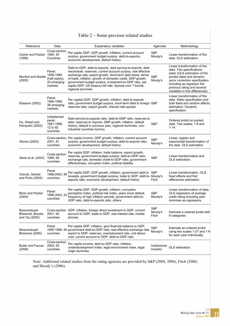
Table 2 – Some previous related studies

Reference Data Explanatory variables Agencies Methodology

Cantor and Packer (1996)

Cross-section, 1995, 45 Countries

Per capita GDP, GDP growth, Inflation, current account surplus, government budget surplus, debt-to-exports, economic development, default history

S&P Moody′s

Linear transformation of the data. OLS estimation.

Monfort and Mulder (2000)

Panel, 1995-1999 (half-yearly), 20 emerging markets

Debt-to-GDP, debt-to-exports, debt service-to-exports, debt reschedule, reserves, current account surplus, real effective exchange rate, export growth, short-term debt share, terms of trade, inflation, growth of domestic credit, GDP growth, government budget surplus, investment-to-GDP ratio, per capita GDP, US treasury bill rate, Spread over T-bonds, regional dummies

S&P Moody′s

Linear transformation of the data. Two specifications: static (OLS estimation of the pooled data) and dynamic (error correction specification including as regressor the previous rating and several variables in first differences)

Eliasson (2002)

Panel, 1990-1999, 38 emerging markets

Per capital GDP, GDP growth, inflation, debt-to-exports ratio, government budget surplus, short-term debt to foreign reserves ratio, export growth, interest rate spread

S&P

Linear transformation of the data. Static specification and both fixed and random effects estimation. Dynamic specification.

Hu, Kiesel and Perraudin (2002)

Unbalanced panel, 1981-1998, 12 to 92 countries

Debt service-to-exports ratio, debt-to-GNP ratio, reserves to debt, reserves to imports, GNP growth, inflation, default history, default in previous year, regional dummies, non-industrial countries dummy

S&P Ordered probit on pooled data. Two scales: 1-8 and 1-14

Afonso (2003) Cross-section, 2001, 81 countries

Per capita income, GDP growth, inflation, current account surplus, government budget surplus, debt-to-exports ratio, economic development, default history

S&P Moody′s

Linear, logistic and exponential transformation of the data. OLS estimation.

Alexe et al. (2003)

Cross-section 1998, 68 countries

Per capita GDP, inflation, trade balance, export growth, reserves, government budget surplus, debt-to-GDP ratio, exchange rate, domestic credit-to-GDP ratio, government effectiveness, corruption index, political stability

S&P Linear transformation and OLS estimation.

Canuto, Santos and Porto (2004)

Panel 1998-2002, 66 countries

Per capita GDP, GDP growth, inflation, government debt to receipts, government budget surplus, trade to GDP, debt-to-exports ratio, economic development, default history

S&P Moody′s Fitch

Linear transformation. OLS, fixed effects and first differences estimation.

Borio and Packer (2004)


Per capita GDP, GDP growth, inflation, corruption perception index, political risk index, years since default, frequency of high inflation periods, government debt-to-GDP ratio, debt-to-exports ratio, others

S&P Moody′s

Linear transformation of data. OLS regression of average credit rating including year dummies as regressors.

Bissoondoyal-Bheenick, Brooks and Yip (2005)


GDP, inflation, foreign direct investment to GDP, current account to GDP, trade to GDP, real interest rate, mobile phones

S&P Moody′s Fitch

Estimate a ordered probit with 9 categories

Bissoondoyal-Bheenick (2005)


Per capita GDP, inflation, govt financial balance to GDP, government debt-to-GDP ratio, real effective exchange rate, export to GDP, reserves, unemployment rate, unit labour cost, current account to GDP, debt-to-GDP ratio

S&P Moody′s

Estimate an ordered probit using two scales 1-21 and 1-9 for each year individually.

Butler and Fauver (2006)


Per capita income, debt-to-GDP ratio, inflation, underdevelopment index, legal environment index, legal origin dummies

Institutional Investor OLS estimation.

Note: Additional related studies from the rating agencies are provided by S&P (2004, 2006), Fitch (2006) and Moody’s (2006).

35ECB


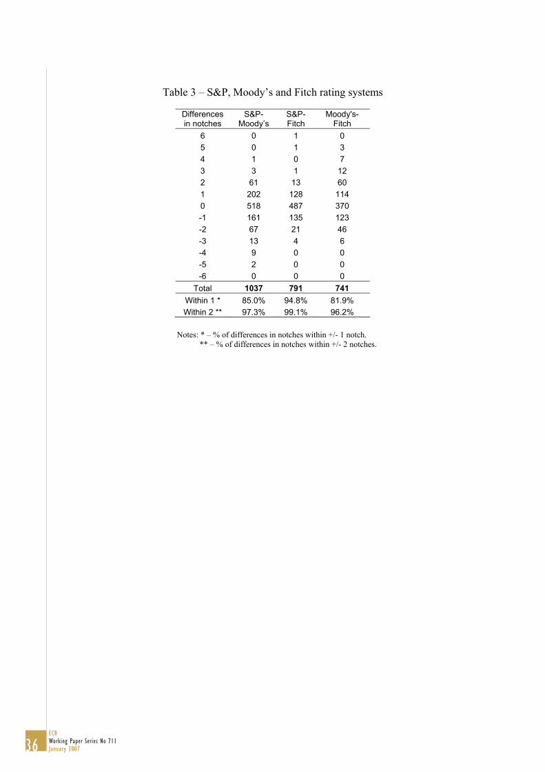
Table 3 – S&P, Moody’s and Fitch rating systems

Differences in notches

S&P-Moody’s

S&P-Fitch

Moody's-Fitch

6 0 1 0 5 0 1 3 4 1 0 7 3 3 1 12 2 61 13 60 1 202 128 114 0 518 487 370 -1 161 135 123 -2 67 21 46 -3 13 4 6 -4 9 0 0 -5 2 0 0 -6 0 0 0

Total 1037 791 741 Within 1 * 85.0% 94.8% 81.9% Within 2 ** 97.3% 99.1% 96.2%

Notes: * – % of differences in notches within +/- 1 notch. ** – % of differences in notches within +/- 2 notches.


Table 4 – Estimations for Moody’s Pooled OLS Random Effects Fixed Effects (1) (2) (3) (4) (5) (6)

Constant 3.618*** 3.934*** 3.431 8.291 10.064*** 9.952 (2.85) (3.22) (0.95) (12.49) (99.36) (143.93) GDP per capita 1.686*** 1.607*** 1.779*** 1.789*** 1.800*** 1.876 (5.07) (4.91) (7.61) (8.03) (7.53) (9.61) GDP per capita Avg. 0.664*** 0.631*** 0.650 (4.11) (3.92) (1.46) GDP growth 7.431*** 9.044*** 8.643*** 8.768*** 8.971*** 5.909 (2.04) (2.76) (3.07) (3.26) (3.14) (2.44) GDP growth Avg. 0.527 5.237 (0.12) (0.46) Unemployment -0.044 -0.069** 0.014 0.024 (-1.43) (-2.34) (0.52) (0.87) Unemployment Avg. -0.049*** -0.051*** -0.072* -0.073* (-3.68) (-3.67) (-1.78) (-1.70) Inflation -0.452*** -0.497*** -0.124* -0.145** -0.105** -0.136 (-2.64) (-2.95) (-1.79) (-2.11) (-2.01) (-2.66) Inflation Avg. -0.648*** -0.712**** -0.360* -0.347** (-3.55) (-4.05) (-1.84) (-2.00) Gov Debt -0.008 -0.014** -0.014** -0.014** -0.016*** -0.015 (-1.21) (-2.40) (-2.38) (-2.53) (-2.65) (-3.54) Gov Debt Avg. -0.013*** -0.016*** -0.011 -0.014** (-4.12) (-4.81) (-1.49) (-2.24) Gov Balance 6.995* 7.740*** 6.991*** 7.598*** 6.056 (1.94) (2.77) (2.54) (2.58) (2.99) Gov Balance Avg. 6.311* 6.122* 7.893 (1.80) (1.67) (0.80) Gov Effectiveness 0.277 0.242 0.205 0.542 (0.88) (1.18) (0.98) (2.90) Gov Effectiveness Avg. 1.927*** 1.756*** 1.906*** 2.470*** (10.89) (9.78) (4.06) (6.80) External Debt -0.010*** -0.009*** -0.004* -0.004* -0.003 (-5.84) (-5.60) (-1.79) (-1.95) (-1.27) External Debt Avg. -0.007*** -0.006*** -0.004** -0.004** (-6.54) (-5.82) (-2.20) (-2.47) Current Account -8.334*** -8.881*** -7.246*** -8.760*** -7.074*** -2.605 (-3.84) (-4.27) (-3.67) (-4.84) (-3.37) (-1.96) Current Account Avg. -1.320 -3.321 (-0.77) (-0.78) Reserves 1.689*** 1.891*** 1.423** 1.710*** 1.488*** 1.132 (3.02) (3.52) (3.63) (4.61) (3.84) (3.56) Reserves Avg. 1.758*** 1.788*** 1.475 1.254 (3.85) (4.03) (1.60) (1.43) Def 1 -1.667*** -1.671*** -1.998*** -2.075*** -2.109*** -2.244 (-6.19) (-6.72) (-6.87) (-8.11) (-6.77) (-7.71) Def 2 0.065*** 0.089*** -0.015 -0.049 (2.67) (3.88) (-0.32) (-0.76) EU (2) 1.220*** 1.273*** 1.598*** 1.650*** 1.704*** 1.376 (6.97) (7.22) (6.63) (6.69) (6.84) (6.51) IND 2.176*** 2.653*** 2.289*** 3.157*** (6.08) (7.57) (2.89) (4.61) LAC -1.072*** -1.282*** -0.903* (-5.44) (-6.39) (-1.93) R2 0.950 0.948 0.945 0.940 0.984 0.980 Countries 66 66 66 66 66 78 Observations 551 557 551 557 551 699 Hausman Test$ 21.93 (0.06) 14.30 (0.160)

Notes: White diagonal standard errors & covariance (d.f. corrected). The t statistics are in parentheses. *, **, *** - statistically significant at the 10, 5, and 1 per cent. $ The null is that RE estimation is consistent and therefore preferable to fixed effects. The test statistic is to be compared to a Qui-Square with 13 and 10 degrees of freedom respectively (the number of time-varying regressors). The p-value is in brackets.

37ECB


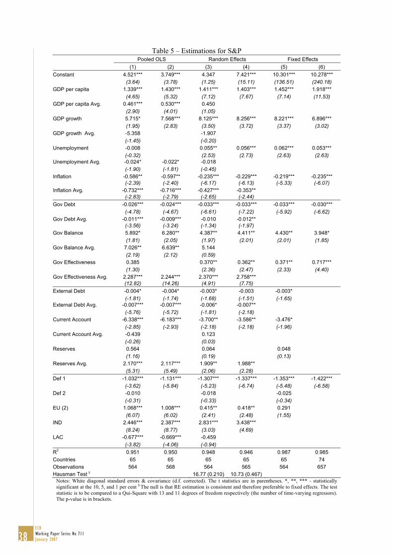
Table 5 – Estimations for S&P Pooled OLS Random Effects Fixed Effects (1) (2) (3) (4) (5) (6) Constant 4.521*** 3.749*** 4.347 7.421*** 10.301*** 10.278*** (3.64) (3.78) (1.25) (15.11) (136.51) (240.18) GDP per capita 1.339*** 1.430*** 1.411*** 1.403*** 1.452*** 1.918*** (4.65) (5.32) (7.12) (7.67) (7.14) (11.53) GDP per capita Avg. 0.461*** 0.530*** 0.450 (2.90) (4.01) (1.05) GDP growth 5.715* 7.568*** 8.125*** 8.256*** 8.221*** 6.896*** (1.95) (2.83) (3.50) (3.72) (3.37) (3.02) GDP growth Avg. -5.358 -1.907 (-1.45) (-0.20) Unemployment -0.008 0.055** 0.056*** 0.062*** 0.053*** (-0.32) (2.53) (2.73) (2.63) (2.63) Unemployment Avg. -0.024* -0.022* -0.018 (-1.90) (-1.81) (-0.45) Inflation -0.586** -0.597** -0.235*** -0.229*** -0.219*** -0.235*** (-2.39) (-2.40) (-6.17) (-6.13) (-5.33) (-6.07) Inflation Avg. -0.732*** -0.716*** -0.427*** -0.353** (-2.83) (-2.79) (-2.65) (-2.44) Gov Debt -0.026*** -0.024*** -0.033*** -0.033*** -0.033*** -0.030*** (-4.78) (-4.67) (-6.61) (-7.22) (-5.92) (-6.62) Gov Debt Avg. -0.011*** -0.009*** -0.010 -0.012** (-3.56) (-3.24) (-1.34) (-1.97) Gov Balance 5.892* 6.280** 4.387** 4.411** 4.430** 3.948* (1.81) (2.05) (1.97) (2.01) (2.01) (1.85) Gov Balance Avg. 7.026** 6.639** 5.144 (2.19) (2.12) (0.59) Gov Effectiveness 0.385 0.370** 0.362** 0.371** 0.717*** (1.30) (2.36) (2.47) (2.33) (4.40) Gov Effectiveness Avg. 2.287*** 2.244*** 2.370*** 2.758*** (12.82) (14.26) (4.91) (7.75) External Debt -0.004* -0.004* -0.003* -0.003 -0.003* (-1.81) (-1.74) (-1.68) (-1.51) (-1.65) External Debt Avg. -0.007*** -0.007*** -0.006* -0.007** (-5.76) (-5.72) (-1.81) (-2.18) Current Account -6.338*** -6.183*** -3.700** -3.586** -3.476* (-2.85) (-2.93) (-2.18) (-2.18) (-1.96) Current Account Avg. -0.439 0.123 (-0.26) (0.03) Reserves 0.564 0.064 0.048 (1.16) (0.19) (0.13) Reserves Avg. 2.170*** 2.117*** 1.909** 1.988** (5.31) (5.49) (2.06) (2.28) Def 1 -1.032*** -1.131*** -1.307*** -1.337*** -1.353*** -1.422*** (-3.62) (-5.84) (-5.23) (-6.74) (-5.48) (-6.58) Def 2 -0.010 -0.018 -0.025 (-0.31) (-0.33) (-0.34) EU (2) 1.068*** 1.008*** 0.415** 0.418** 0.291 (6.07) (6.02) (2.41) (2.48) (1.55) IND 2.446*** 2.387*** 2.831*** 3.438*** (8.24) (8.77) (3.03) (4.69) LAC -0.677*** -0.669*** -0.459 (-3.82) (-4.06) (-0.94) R2 0.951 0.950 0.948 0.946 0.987 0.985 Countries 65 65 65 65 65 74 Observations 564 568 564 565 564 657 Hausman Test $ 16.77 (0.210) 10.73 (0.467)

Notes: White diagonal standard errors & covariance (d.f. corrected). The t statistics are in parentheses. *, **, *** - statistically significant at the 10, 5, and 1 per cent $ The null is that RE estimation is consistent and therefore preferable to fixed effects. The test statistic is to be compared to a Qui-Square with 13 and 11 degrees of freedom respectively (the number of time-varying regressors). The p-value is in brackets.


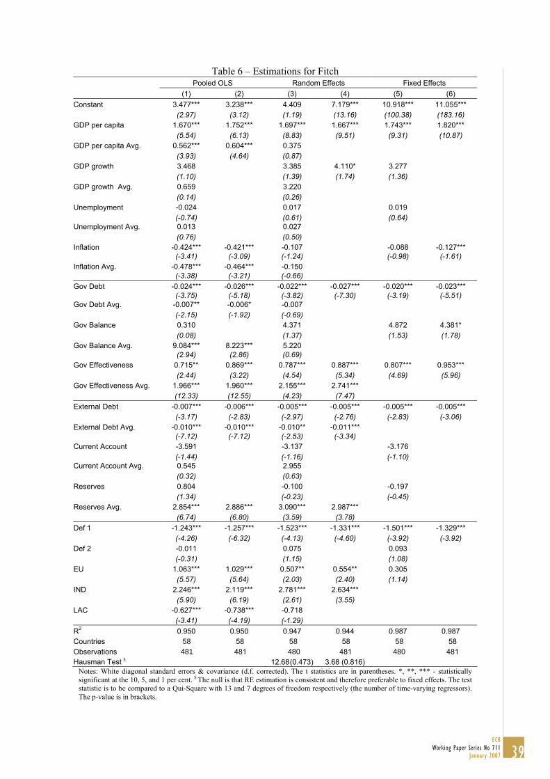
Table 6 – Estimations for Fitch Pooled OLS Random Effects Fixed Effects (1) (2) (3) (4) (5) (6)

Constant 3.477*** 3.238*** 4.409 7.179*** 10.918*** 11.055*** (2.97) (3.12) (1.19) (13.16) (100.38) (183.16) GDP per capita 1.670*** 1.752*** 1.697*** 1.667*** 1.743*** 1.820*** (5.54) (6.13) (8.83) (9.51) (9.31) (10.87) GDP per capita Avg. 0.562*** 0.604*** 0.375 (3.93) (4.64) (0.87) GDP growth 3.468 3.385 4.110* 3.277 (1.10) (1.39) (1.74) (1.36) GDP growth Avg. 0.659 3.220 (0.14) (0.26) Unemployment -0.024 0.017 0.019 (-0.74) (0.61) (0.64) Unemployment Avg. 0.013 0.027 (0.76) (0.50) Inflation -0.424*** -0.421*** -0.107 -0.088 -0.127*** (-3.41) (-3.09) (-1.24) (-0.98) (-1.61) Inflation Avg. -0.478*** -0.464*** -0.150 (-3.38) (-3.21) (-0.66) Gov Debt -0.024*** -0.026*** -0.022*** -0.027*** -0.020*** -0.023*** (-3.75) (-5.18) (-3.82) (-7.30) (-3.19) (-5.51) Gov Debt Avg. -0.007** -0.006* -0.007 (-2.15) (-1.92) (-0.69) Gov Balance 0.310 4.371 4.872 4.381* (0.08) (1.37) (1.53) (1.78) Gov Balance Avg. 9.084*** 8.223*** 5.220 (2.94) (2.86) (0.69) Gov Effectiveness 0.715** 0.869*** 0.787*** 0.887*** 0.807*** 0.953*** (2.44) (3.22) (4.54) (5.34) (4.69) (5.96) Gov Effectiveness Avg. 1.966*** 1.960*** 2.155*** 2.741*** (12.33) (12.55) (4.23) (7.47) External Debt -0.007*** -0.006*** -0.005*** -0.005*** -0.005*** -0.005*** (-3.17) (-2.83) (-2.97) (-2.76) (-2.83) (-3.06) External Debt Avg. -0.010*** -0.010*** -0.010** -0.011*** (-7.12) (-7.12) (-2.53) (-3.34) Current Account -3.591 -3.137 -3.176 (-1.44) (-1.16) (-1.10) Current Account Avg. 0.545 2.955 (0.32) (0.63) Reserves 0.804 -0.100 -0.197 (1.34) (-0.23) (-0.45) Reserves Avg. 2.854*** 2.886*** 3.090*** 2.987*** (6.74) (6.80) (3.59) (3.78) Def 1 -1.243*** -1.257*** -1.523*** -1.331*** -1.501*** -1.329*** (-4.26) (-6.32) (-4.13) (-4.60) (-3.92) (-3.92) Def 2 -0.011 0.075 0.093 (-0.31) (1.15) (1.08) EU 1.063*** 1.029*** 0.507** 0.554** 0.305 (5.57) (5.64) (2.03) (2.40) (1.14) IND 2.246*** 2.119*** 2.781*** 2.634*** (5.90) (6.19) (2.61) (3.55) LAC -0.627*** -0.738*** -0.718 (-3.41) (-4.19) (-1.29) R2 0.950 0.950 0.947 0.944 0.987 0.987 Countries 58 58 58 58 58 58 Observations 481 481 480 481 480 481 Hausman Test $ 12.68 (0.473) 3.68 (0.816)

Notes: White diagonal standard errors & covariance (d.f. corrected). The t statistics are in parentheses. *, **, *** - statistically significant at the 10, 5, and 1 per cent. $ The null is that RE estimation is consistent and therefore preferable to fixed effects. The test statistic is to be compared to a Qui-Square with 13 and 7 degrees of freedom respectively (the number of time-varying regressors). The p-value is in brackets.

39ECB


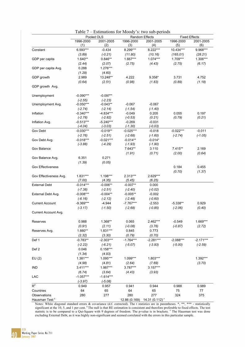
Table 7 – Estimations for Moody’s: two sub-periods Pooled OLS Random Effects Fixed Effects

1996-2000

(1) 2001-2005

(2) 1996-2000

(3) 2001-2005

(4) 1996-2000

(5) 2001-2005

(6) Constant 6.593*** -0.434 8.299*** 8.222*** 10.434*** 9.968*** (3.89) (-0.21) (11.80) (10.16) (165.01) (28.21) GDP per capita 1.640** 0.846** 1.667*** 1.074*** 1.709*** 1.306*** (2.44) (2.07) (2.75) (4.43) (2.75) (6.17) GDP per capita Avg. 0.288 1.276*** (1.29) (4.60) GDP growth 2.989 13.248** 4.222 9.358* 3.731 4.752 (0.64) (2.51) (0.98) (1.83) (0.89) (1.18) GDP growth Avg. Unemployment -0.090*** -0.097** (-2.55) (-2.23) Unemployment Avg. -0.050*** -0.043** -0.067 -0.067 (-2.74) (-2.14) (-1.54) (-1.40) Inflation -0.340*** -4.834*** -0.049 0.205 0.055 0.197 (-2.78) (-2.82) (-0.53) (0.21) (0.79) (0.21) Inflation Avg. -0.513*** -5.240*** -0.269 -0.031 (-4.04) (-3.03) (-1.30) (-0.03) Gov Debt -0.030*** -0.019** -0.025*** -0.018 -0.022*** -0.011 (-2.76) (-2.51) (-2.68) (-1.60) (-2.74) (-1.05) Gov Debt Avg. -0.018*** -0.021*** -0.014** -0.014* (-3.88) (-4.29) (-1.93) (-1.90) Gov Balance 7.643** 3.110 7.415** 2.169 (1.91) (0.71) (2.00) (0.64) Gov Balance Avg. 6.351 0.271 (1.39) (0.05) Gov Effectiveness 0.184 0.455 (0.70) (1.37) Gov Effectiveness Avg. 1.831*** 1.198*** 2.313*** 2.629*** (7.00) (4.35) (5.45) (6.25) External Debt -0.014*** -0.006** -0.007** 0.000 (-7.38) (-2.51) (-2.40) (-0.02) External Debt Avg. -0.008*** -0.004** -0.005** -0.002 (-6.16) (-2.12) (-2.48) (-0.60) Current Account -9.369*** -4.944 -7.767*** -2.553 -5.338** 0.929 (-3.17) (-1.50) (-2.68) (-0.85) (-2.06) (0.40) Current Account Avg. Reserves 0.988 1.368** 0.065 2.462*** -0.549 1.669*** (0.91) (2.11) (-0.08) (3.76) (-0.87) (2.72) Reserves Avg. 1.660** 1.831*** 0.845 0.773 (2.32) (3.30) (0.79) (0.70) Def 1 -0.783** -2.303*** -1.764*** -2.281*** -2.088*** -2.171*** (-2.22) (-6.21) (-5.07) (-3.93) (-5.00) (-2.59) Def 2 0.046 0.158*** (1.34) (4.93) EU (2) 1.381*** 1.095*** 1.099*** 1.803*** 1.392*** (4.98) (4.81) (2.64) (7.69) (3.70) IND 3.411*** 1.987*** 3.787*** 3.157*** (6.74) (3.64) (4.43) (3.93) LAC -1.057*** -1.614*** (-3.97) (-5.08) R2 0.949 0.957 0.941 0.944 0.988 0.989 Countries 64 65 64 65 75 77 Observations 280 277 280 277 324 375 Hausman Test $ 12.86 (0.169) 14.31 (0.112) #

Notes: White diagonal standard errors & covariance (d.f. corrected). The t statistics are in parentheses. *, **, *** - statistically significant at the 10, 5, and 1 per cent. $ The null is that RE estimation is consistent and therefore preferable to fixed effects. The test statistic is to be compared to a Qui-Square with 9 degrees of freedom. The p-value is in brackets. # The Hausman test was done excluding External Debt, as it was highly non-significant and seemed correlated with the errors in this particular sample.


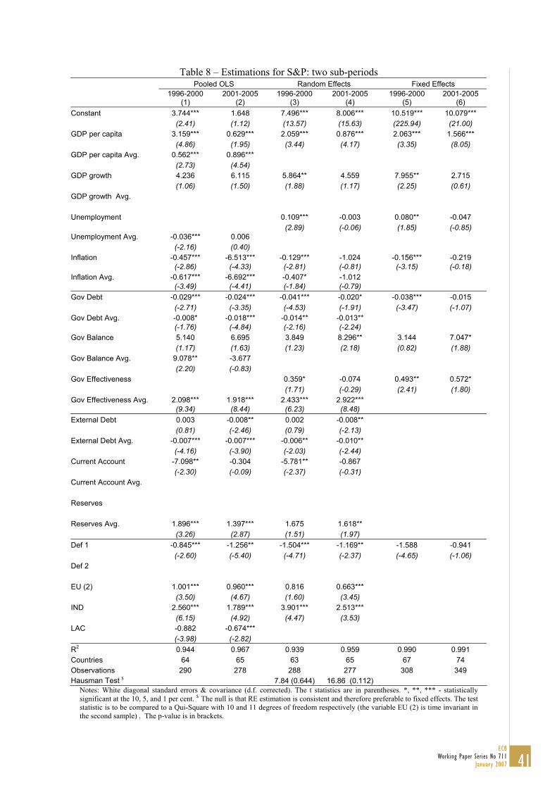
Table 8 – Estimations for S&P: two sub-periods Pooled OLS Random Effects Fixed Effects

1996-2000

(1) 2001-2005

(2) 1996-2000

(3) 2001-2005

(4) 1996-2000

(5) 2001-2005

(6) Constant 3.744*** 1.648 7.496*** 8.006*** 10.519*** 10.079*** (2.41) (1.12) (13.57) (15.63) (225.94) (21.00) GDP per capita 3.159*** 0.629*** 2.059*** 0.876*** 2.063*** 1.566*** (4.86) (1.95) (3.44) (4.17) (3.35) (8.05) GDP per capita Avg. 0.562*** 0.896*** (2.73) (4.54) GDP growth 4.236 6.115 5.864** 4.559 7.955** 2.715 (1.06) (1.50) (1.88) (1.17) (2.25) (0.61) GDP growth Avg. Unemployment 0.109*** -0.003 0.080** -0.047 (2.89) (-0.06) (1.85) (-0.85) Unemployment Avg. -0.036*** 0.006 (-2.16) (0.40) Inflation -0.457*** -6.513*** -0.129*** -1.024 -0.156*** -0.219 (-2.86) (-4.33) (-2.81) (-0.81) (-3.15) (-0.18) Inflation Avg. -0.617*** -6.692*** -0.407* -1.012 (-3.49) (-4.41) (-1.84) (-0.79) Gov Debt -0.029*** -0.024*** -0.041*** -0.020* -0.038*** -0.015 (-2.71) (-3.35) (-4.53) (-1.91) (-3.47) (-1.07) Gov Debt Avg. -0.008* -0.018*** -0.014** -0.013** (-1.76) (-4.84) (-2.16) (-2.24) Gov Balance 5.140 6.695 3.849 8.296** 3.144 7.047* (1.17) (1.63) (1.23) (2.18) (0.82) (1.88) Gov Balance Avg. 9.078** -3.677 (2.20) (-0.83) Gov Effectiveness 0.359* -0.074 0.493** 0.572* (1.71) (-0.29) (2.41) (1.80) Gov Effectiveness Avg. 2.098*** 1.918*** 2.433*** 2.922*** (9.34) (8.44) (6.23) (8.48) External Debt 0.003 -0.008** 0.002 -0.008** (0.81) (-2.46) (0.79) (-2.13) External Debt Avg. -0.007*** -0.007*** -0.006** -0.010** (-4.16) (-3.90) (-2.03) (-2.44) Current Account -7.098** -0.304 -5.781** -0.867 (-2.30) (-0.09) (-2.37) (-0.31) Current Account Avg. Reserves Reserves Avg. 1.896*** 1.397*** 1.675 1.618** (3.26) (2.87) (1.51) (1.97) Def 1 -0.845*** -1.256** -1.504*** -1.169** -1.588 -0.941 (-2.60) (-5.40) (-4.71) (-2.37) (-4.65) (-1.06) Def 2 EU (2) 1.001*** 0.960*** 0.816 0.663*** (3.50) (4.67) (1.60) (3.45) IND 2.560*** 1.789*** 3.901*** 2.513*** (6.15) (4.92) (4.47) (3.53) LAC -0.882 -0.674*** (-3.98) (-2.82) R2 0.944 0.967 0.939 0.959 0.990 0.991 Countries 64 65 63 65 67 74 Observations 290 278 288 277 308 349 Hausman Test $ 7.84 (0.644) 16.86 (0.112)

Notes: White diagonal standard errors & covariance (d.f. corrected). The t statistics are in parentheses. *, **, *** - statistically significant at the 10, 5, and 1 per cent. $ The null is that RE estimation is consistent and therefore preferable to fixed effects. The test statistic is to be compared to a Qui-Square with 10 and 11 degrees of freedom respectively (the variable EU (2) is time invariant in the second sample) . The p-value is in brackets.

41ECB


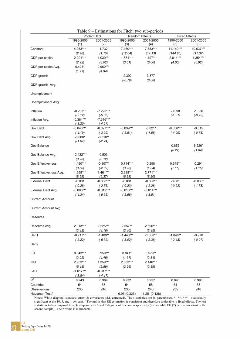
Table 9 – Estimations for Fitch: two sub-periods Pooled OLS Random Effects Fixed Effects

1996-2000

(1) 2001-2005

(2) 1996-2000

(3) 2001-2005

(4) 1996-2000

(5) 2001-2005

(6) Constant 4.953*** 1.732 7.160*** 7.783*** 11.149*** 10.637*** (2.96) (1.15) (12.04) (14.13) (144.80) (17.37) GDP per capita 2.201*** 1.030*** 1.881*** 1.197*** 2.014*** 1.354*** (2.92) (3.02) (3.61) (6.00) (4.00) (5.92) GDP per capita Avg. 0.403* 0.960*** (1.93) (4.94) GDP growth -2.392 3.377 (-0.79) (0.88) GDP growth Avg. Unemployment Unemployment Avg. Inflation -0.233** -7.223*** -0.098 -1.086 (-2.12) (-5.06) (-1.01) (-0.73) Inflation Avg. -0.364*** -7.316*** (-3.20) (-4.97) Gov Debt -0.046*** -0.027*** -0.039*** -0.021* -0.036*** -0.015 (-4.19) (-3.99) (-5.81) (-1.85) (-4.09) (-0.78) Gov Debt Avg. -0.008* -0.010** (-1.67) (-2.24) Gov Balance 0.852 6.226* (0.22) (1.84) Gov Balance Avg. 12.422*** 0.503 (3.26) (0.12) Gov Effectiveness 1.490*** -0.907** 0.714*** 0.298 0.545** 0.294 (3.60) (-2.09) (3.26) (1.04) (2.15) (1.15) Gov Effectiveness Avg. 1.958*** 1.461*** 2.628*** 2.771*** (8.59) (6.37) (6.28) (8.20) External Debt -0.001 -0.008*** -0.001 -0.008** -0.001 -0.008* (-0.28) (-2.76) (-0.23) (-2.26) (-0.22) (-1.78) External Debt Avg. -0.008*** -0.012*** -0.010*** -0.014*** (-4.34) (-5.35) (-2.68) (-3.51) Current Account Current Account Avg. Reserves Reserves Avg. 2.313*** 2.225*** 2.557** 2.696*** (3.42) (4.16) (2.40) (3.45) Def 1 -0.717** -1.409** -1.440*** -1.338** -1.848** -0.970 (-2.22) (-5.32) (-3.02) (-2.36) (-2.43) (-0.97) Def 2 EU 0.843*** 0.959*** 0.841* 0.579** (2.92) (4.45) (1.67) (2.34) IND 2.953*** 1.359*** 2.883*** 2.146*** (5.48) (2.89) (2.96) (3.39) LAC -1.017*** -0.917*** (-3.84) (-4.17) R2 0.943 0.969 0.932 0.957 0.990 0.993 Countries 54 58 54 58 54 58 Observations 235 246 235 246 235 246 Hausman Test $ 6.95 (0.325) 11.25 (0.128)

Notes: White diagonal standard errors & covariance (d.f. corrected). The t statistics are in parentheses. *, **, *** - statistically significant at the 10, 5, and 1 per cent. $ The null is that RE estimation is consistent and therefore preferable to fixed effects. The test statistic is to be compared to a Qui-Square with 8 and 7 degrees of freedom respectively (the variable EU (2) is time invariant in the second sample). The p-value is in brackets.


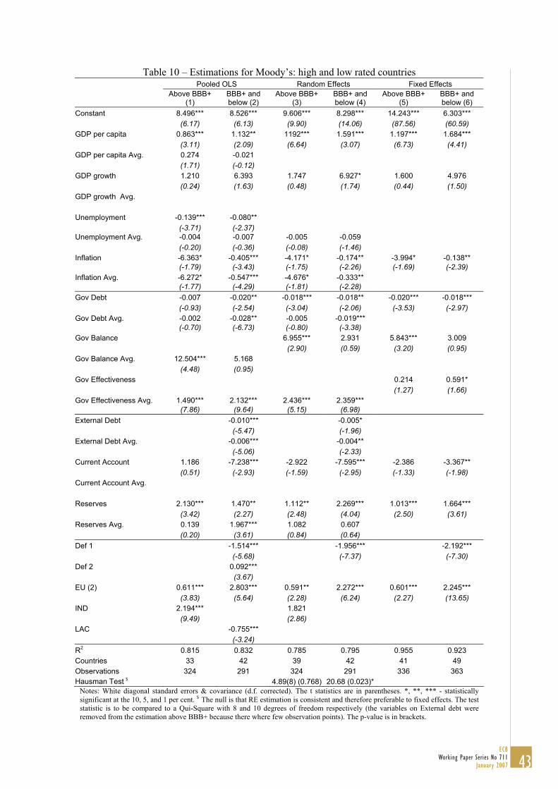
Table 10 – Estimations for Moody’s: high and low rated countries Pooled OLS Random Effects Fixed Effects Above BBB+

(1) BBB+ and below (2)

Above BBB+ (3)

BBB+ and below (4)

Above BBB+ (5)

BBB+ and below (6)

Constant 8.496*** 8.526*** 9.606*** 8.298*** 14.243*** 6.303*** (6.17) (6.13) (9.90) (14.06) (87.56) (60.59) GDP per capita 0.863*** 1.132** 1192*** 1.591*** 1.197*** 1.684*** (3.11) (2.09) (6.64) (3.07) (6.73) (4.41) GDP per capita Avg. 0.274 -0.021 (1.71) (-0.12) GDP growth 1.210 6.393 1.747 6.927* 1.600 4.976 (0.24) (1.63) (0.48) (1.74) (0.44) (1.50) GDP growth Avg. Unemployment -0.139*** -0.080** (-3.71) (-2.37) Unemployment Avg. -0.004 -0.007 -0.005 -0.059 (-0.20) (-0.36) (-0.08) (-1.46) Inflation -6.363* -0.405*** -4.171* -0.174** -3.994* -0.138** (-1.79) (-3.43) (-1.75) (-2.26) (-1.69) (-2.39) Inflation Avg. -6.272* -0.547*** -4.676* -0.333** (-1.77) (-4.29) (-1.81) (-2.28) Gov Debt -0.007 -0.020** -0.018*** -0.018** -0.020*** -0.018*** (-0.93) (-2.54) (-3.04) (-2.06) (-3.53) (-2.97) Gov Debt Avg. -0.002 -0.028** -0.005 -0.019*** (-0.70) (-6.73) (-0.80) (-3.38) Gov Balance 6.955*** 2.931 5.843*** 3.009 (2.90) (0.59) (3.20) (0.95) Gov Balance Avg. 12.504*** 5.168 (4.48) (0.95) Gov Effectiveness 0.214 0.591* (1.27) (1.66) Gov Effectiveness Avg. 1.490*** 2.132*** 2.436*** 2.359*** (7.86) (9.64) (5.15) (6.98) External Debt -0.010*** -0.005* (-5.47) (-1.96) External Debt Avg. -0.006*** -0.004** (-5.06) (-2.33) Current Account 1.186 -7.238*** -2.922 -7.595*** -2.386 -3.367** (0.51) (-2.93) (-1.59) (-2.95) (-1.33) (-1.98) Current Account Avg. Reserves 2.130*** 1.470** 1.112** 2.269*** 1.013*** 1.664*** (3.42) (2.27) (2.48) (4.04) (2.50) (3.61) Reserves Avg. 0.139 1.967*** 1.082 0.607 (0.20) (3.61) (0.84) (0.64) Def 1 -1.514*** -1.956*** -2.192*** (-5.68) (-7.37) (-7.30) Def 2 0.092*** (3.67) EU (2) 0.611*** 2.803*** 0.591** 2.272*** 0.601*** 2.245*** (3.83) (5.64) (2.28) (6.24) (2.27) (13.65) IND 2.194*** 1.821 (9.49) (2.86) LAC -0.755*** (-3.24) R2 0.815 0.832 0.785 0.795 0.955 0.923 Countries 33 42 39 42 41 49 Observations 324 291 324 291 336 363 Hausman Test $ 4.89(8) (0.768) 20.68 (0.023)*

Notes: White diagonal standard errors & covariance (d.f. corrected). The t statistics are in parentheses. *, **, *** - statistically significant at the 10, 5, and 1 per cent. $ The null is that RE estimation is consistent and therefore preferable to fixed effects. The test statistic is to be compared to a Qui-Square with 8 and 10 degrees of freedom respectively (the variables on External debt were removed from the estimation above BBB+ because there where few observation points). The p-value is in brackets.

43ECB


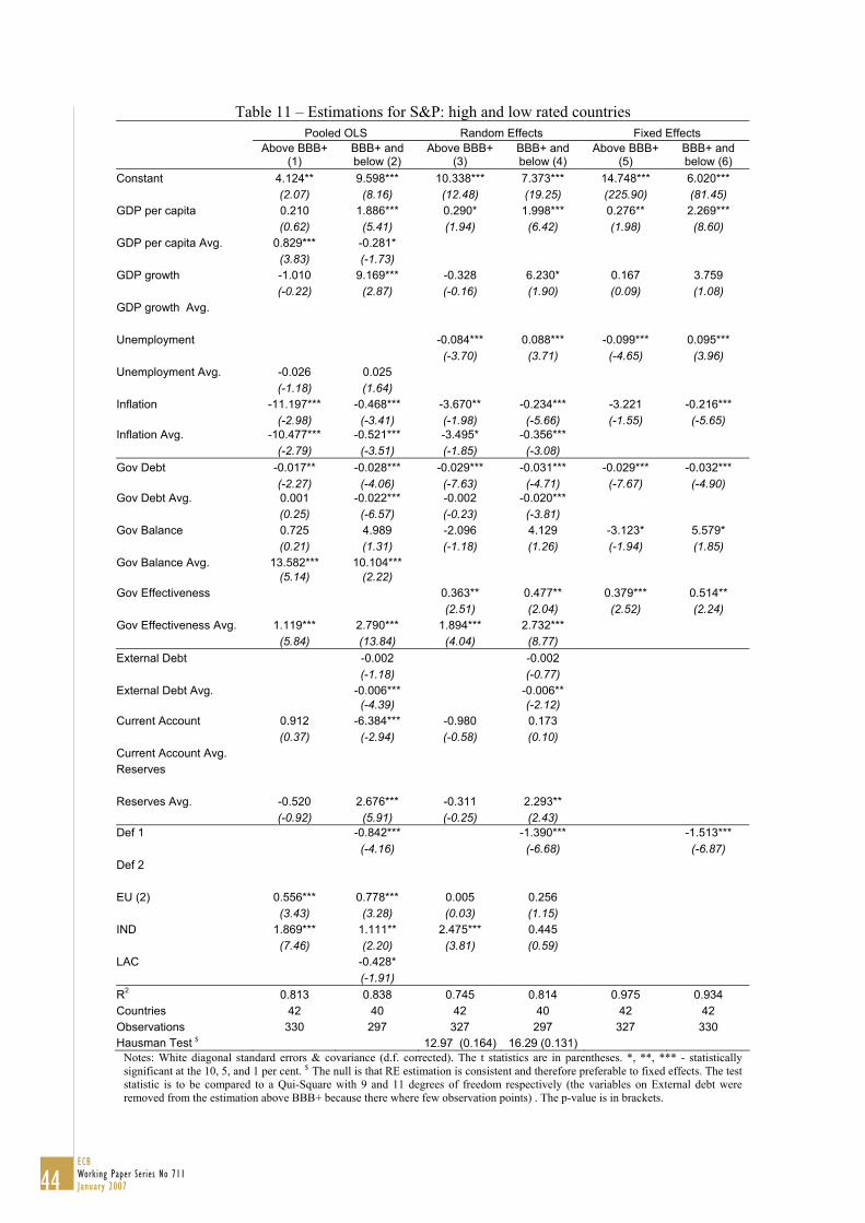
Table 11 – Estimations for S&P: high and low rated countries Pooled OLS Random Effects Fixed Effects Above BBB+


Above BBB+ (3)

BBB+ and below (4)

Above BBB+ (5)

BBB+ and below (6)

Constant 4.124** 9.598*** 10.338*** 7.373*** 14.748*** 6.020*** (2.07) (8.16) (12.48) (19.25) (225.90) (81.45) GDP per capita 0.210 1.886*** 0.290* 1.998*** 0.276** 2.269*** (0.62) (5.41) (1.94) (6.42) (1.98) (8.60) GDP per capita Avg. 0.829*** -0.281* (3.83) (-1.73) GDP growth -1.010 9.169*** -0.328 6.230* 0.167 3.759 (-0.22) (2.87) (-0.16) (1.90) (0.09) (1.08) GDP growth Avg. Unemployment -0.084*** 0.088*** -0.099*** 0.095*** (-3.70) (3.71) (-4.65) (3.96) Unemployment Avg. -0.026 0.025 (-1.18) (1.64) Inflation -11.197*** -0.468*** -3.670** -0.234*** -3.221 -0.216*** (-2.98) (-3.41) (-1.98) (-5.66) (-1.55) (-5.65) Inflation Avg. -10.477*** -0.521*** -3.495* -0.356*** (-2.79) (-3.51) (-1.85) (-3.08) Gov Debt -0.017** -0.028*** -0.029*** -0.031*** -0.029*** -0.032*** (-2.27) (-4.06) (-7.63) (-4.71) (-7.67) (-4.90) Gov Debt Avg. 0.001 -0.022*** -0.002 -0.020*** (0.25) (-6.57) (-0.23) (-3.81) Gov Balance 0.725 4.989 -2.096 4.129 -3.123* 5.579* (0.21) (1.31) (-1.18) (1.26) (-1.94) (1.85) Gov Balance Avg. 13.582*** 10.104*** (5.14) (2.22) Gov Effectiveness 0.363** 0.477** 0.379*** 0.514** (2.51) (2.04) (2.52) (2.24) Gov Effectiveness Avg. 1.119*** 2.790*** 1.894*** 2.732*** (5.84) (13.84) (4.04) (8.77) External Debt -0.002 -0.002 (-1.18) (-0.77) External Debt Avg. -0.006*** -0.006** (-4.39) (-2.12) Current Account 0.912 -6.384*** -0.980 0.173 (0.37) (-2.94) (-0.58) (0.10) Current Account Avg. Reserves Reserves Avg. -0.520 2.676*** -0.311 2.293** (-0.92) (5.91) (-0.25) (2.43) Def 1 -0.842*** -1.390*** -1.513*** (-4.16) (-6.68) (-6.87) Def 2 EU (2) 0.556*** 0.778*** 0.005 0.256 (3.43) (3.28) (0.03) (1.15) IND 1.869*** 1.111** 2.475*** 0.445 (7.46) (2.20) (3.81) (0.59) LAC -0.428* (-1.91) R2 0.813 0.838 0.745 0.814 0.975 0.934 Countries 42 40 42 40 42 42 Observations 330 297 327 297 327 330 Hausman Test $ 12.97 (0.164) 16.29 (0.131)

Notes: White diagonal standard errors & covariance (d.f. corrected). The t statistics are in parentheses. *, **, *** - statistically significant at the 10, 5, and 1 per cent. $ The null is that RE estimation is consistent and therefore preferable to fixed effects. The test statistic is to be compared to a Qui-Square with 9 and 11 degrees of freedom respectively (the variables on External debt were removed from the estimation above BBB+ because there where few observation points) . The p-value is in brackets.


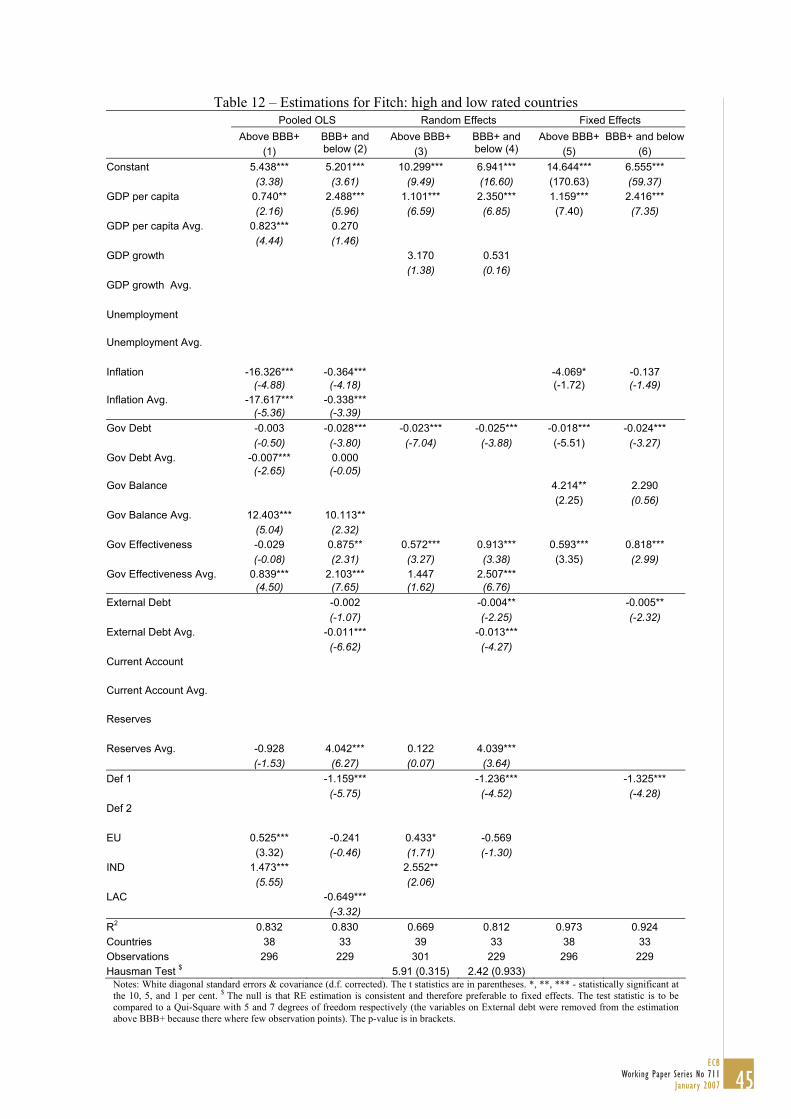
Table 12 – Estimations for Fitch: high and low rated countries Pooled OLS Random Effects Fixed Effects Above BBB+


Above BBB+ (3)

BBB+ and below (4)

Above BBB+ (5)

BBB+ and below(6)

Constant 5.438*** 5.201*** 10.299*** 6.941*** 14.644*** 6.555*** (3.38) (3.61) (9.49) (16.60) (170.63) (59.37) GDP per capita 0.740** 2.488*** 1.101*** 2.350*** 1.159*** 2.416*** (2.16) (5.96) (6.59) (6.85) (7.40) (7.35) GDP per capita Avg. 0.823*** 0.270 (4.44) (1.46) GDP growth 3.170 0.531 (1.38) (0.16) GDP growth Avg. Unemployment Unemployment Avg. Inflation -16.326*** -0.364*** -4.069* -0.137 (-4.88) (-4.18) (-1.72) (-1.49) Inflation Avg. -17.617*** -0.338*** (-5.36) (-3.39) Gov Debt -0.003 -0.028*** -0.023*** -0.025*** -0.018*** -0.024*** (-0.50) (-3.80) (-7.04) (-3.88) (-5.51) (-3.27) Gov Debt Avg. -0.007*** 0.000 (-2.65) (-0.05) Gov Balance 4.214** 2.290 (2.25) (0.56) Gov Balance Avg. 12.403*** 10.113** (5.04) (2.32) Gov Effectiveness -0.029 0.875** 0.572*** 0.913*** 0.593*** 0.818*** (-0.08) (2.31) (3.27) (3.38) (3.35) (2.99) Gov Effectiveness Avg. 0.839*** 2.103*** 1.447 2.507*** (4.50) (7.65) (1.62) (6.76) External Debt -0.002 -0.004** -0.005** (-1.07) (-2.25) (-2.32) External Debt Avg. -0.011*** -0.013*** (-6.62) (-4.27) Current Account Current Account Avg. Reserves Reserves Avg. -0.928 4.042*** 0.122 4.039*** (-1.53) (6.27) (0.07) (3.64) Def 1 -1.159*** -1.236*** -1.325*** (-5.75) (-4.52) (-4.28) Def 2 EU 0.525*** -0.241 0.433* -0.569 (3.32) (-0.46) (1.71) (-1.30) IND 1.473*** 2.552** (5.55) (2.06) LAC -0.649*** (-3.32) R2 0.832 0.830 0.669 0.812 0.973 0.924 Countries 38 33 39 33 38 33 Observations 296 229 301 229 296 229 Hausman Test $ 5.91 (0.315) 2.42 (0.933)

Notes: White diagonal standard errors & covariance (d.f. corrected). The t statistics are in parentheses. *, **, *** - statistically significant at the 10, 5, and 1 per cent. $ The null is that RE estimation is consistent and therefore preferable to fixed effects. The test statistic is to be compared to a Qui-Square with 5 and 7 degrees of freedom respectively (the variables on External debt were removed from the estimation above BBB+ because there where few observation points). The p-value is in brackets.

45ECB


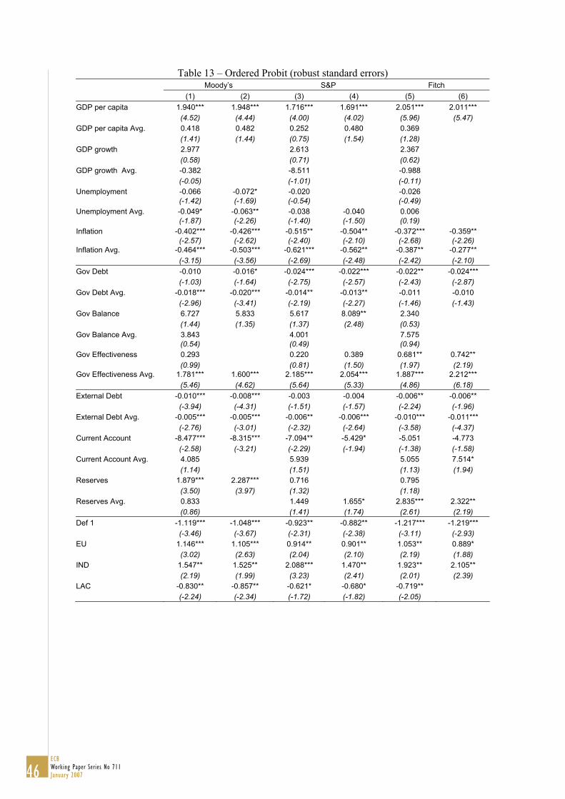
Table 13 – Ordered Probit (robust standard errors) Moody’s S&P Fitch (1) (2) (3) (4) (5) (6)

GDP per capita 1.940*** 1.948*** 1.716*** 1.691*** 2.051*** 2.011*** (4.52) (4.44) (4.00) (4.02) (5.96) (5.47) GDP per capita Avg. 0.418 0.482 0.252 0.480 0.369 (1.41) (1.44) (0.75) (1.54) (1.28) GDP growth 2.977 2.613 2.367 (0.58) (0.71) (0.62) GDP growth Avg. -0.382 -8.511 -0.988 (-0.05) (-1.01) (-0.11) Unemployment -0.066 -0.072* -0.020 -0.026 (-1.42) (-1.69) (-0.54) (-0.49) Unemployment Avg. -0.049* -0.063** -0.038 -0.040 0.006 (-1.87) (-2.26) (-1.40) (-1.50) (0.19) Inflation -0.402*** -0.426*** -0.515** -0.504** -0.372*** -0.359** (-2.57) (-2.62) (-2.40) (-2.10) (-2.68) (-2.26) Inflation Avg. -0.464*** -0.503*** -0.621*** -0.562** -0.387** -0.277** (-3.15) (-3.56) (-2.69) (-2.48) (-2.42) (-2.10) Gov Debt -0.010 -0.016* -0.024*** -0.022*** -0.022** -0.024*** (-1.03) (-1.64) (-2.75) (-2.57) (-2.43) (-2.87) Gov Debt Avg. -0.018*** -0.020*** -0.014** -0.013** -0.011 -0.010 (-2.96) (-3.41) (-2.19) (-2.27) (-1.46) (-1.43) Gov Balance 6.727 5.833 5.617 8.089** 2.340 (1.44) (1.35) (1.37) (2.48) (0.53) Gov Balance Avg. 3.843 4.001 7.575 (0.54) (0.49) (0.94) Gov Effectiveness 0.293 0.220 0.389 0.681** 0.742** (0.99) (0.81) (1.50) (1.97) (2.19) Gov Effectiveness Avg. 1.781*** 1.600*** 2.185*** 2.054*** 1.887*** 2.212*** (5.46) (4.62) (5.64) (5.33) (4.86) (6.18) External Debt -0.010*** -0.008*** -0.003 -0.004 -0.006** -0.006** (-3.94) (-4.31) (-1.51) (-1.57) (-2.24) (-1.96) External Debt Avg. -0.005*** -0.005*** -0.006** -0.006*** -0.010*** -0.011*** (-2.76) (-3.01) (-2.32) (-2.64) (-3.58) (-4.37) Current Account -8.477*** -8.315*** -7.094** -5.429* -5.051 -4.773 (-2.58) (-3.21) (-2.29) (-1.94) (-1.38) (-1.58) Current Account Avg. 4.085 5.939 5.055 7.514* (1.14) (1.51) (1.13) (1.94) Reserves 1.879*** 2.287*** 0.716 0.795 (3.50) (3.97) (1.32) (1.18) Reserves Avg. 0.833 1.449 1.655* 2.835*** 2.322** (0.86) (1.41) (1.74) (2.61) (2.19) Def 1 -1.119*** -1.048*** -0.923** -0.882** -1.217*** -1.219*** (-3.46) (-3.67) (-2.31) (-2.38) (-3.11) (-2.93) EU 1.146*** 1.105*** 0.914** 0.901** 1.053** 0.889* (3.02) (2.63) (2.04) (2.10) (2.19) (1.88) IND 1.547** 1.525** 2.088*** 1.470** 1.923** 2.105** (2.19) (1.99) (3.23) (2.41) (2.01) (2.39) LAC -0.830** -0.857** -0.621* -0.680* -0.719**

(-2.24) (-2.34) (-1.72) (-1.82) (-2.05)


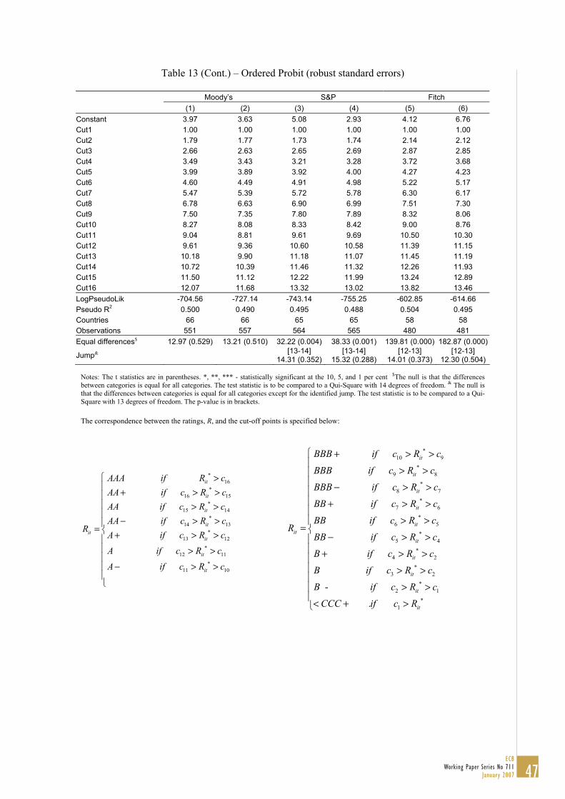
Table 13 (Cont.) – Ordered Probit (robust standard errors)

Moody’s S&P Fitch (1) (2) (3) (4) (5) (6)

Constant 3.97 3.63 5.08 2.93 4.12 6.76 Cut1 1.00 1.00 1.00 1.00 1.00 1.00 Cut2 1.79 1.77 1.73 1.74 2.14 2.12 Cut3 2.66 2.63 2.65 2.69 2.87 2.85 Cut4 3.49 3.43 3.21 3.28 3.72 3.68 Cut5 3.99 3.89 3.92 4.00 4.27 4.23 Cut6 4.60 4.49 4.91 4.98 5.22 5.17 Cut7 5.47 5.39 5.72 5.78 6.30 6.17 Cut8 6.78 6.63 6.90 6.99 7.51 7.30 Cut9 7.50 7.35 7.80 7.89 8.32 8.06 Cut10 8.27 8.08 8.33 8.42 9.00 8.76 Cut11 9.04 8.81 9.61 9.69 10.50 10.30 Cut12 9.61 9.36 10.60 10.58 11.39 11.15 Cut13 10.18 9.90 11.18 11.07 11.45 11.19 Cut14 10.72 10.39 11.46 11.32 12.26 11.93 Cut15 11.50 11.12 12.22 11.99 13.24 12.89 Cut16 12.07 11.68 13.32 13.02 13.82 13.46 LogPseudoLik -704.56 -727.14 -743.14 -755.25 -602.85 -614.66 Pseudo R2 0.500 0.490 0.495 0.488 0.504 0.495 Countries 66 66 65 65 58 58 Observations 551 557 564 565 480 481 Equal differences$ 12.97 (0.529) 13.21 (0.510) 32.22 (0.004) 38.33 (0.001) 139.81 (0.000) 182.87 (0.000)

Jump& [13-14]

14.31 (0.352)[13-14]

15.32 (0.288) [12-13]

14.01 (0.373) [12-13]

12.30 (0.504) Notes: The t statistics are in parentheses. *, **, *** - statistically significant at the 10, 5, and 1 per cent $The null is that the differences between categories is equal for all categories. The test statistic is to be compared to a Qui-Square with 14 degrees of freedom. & The null is that the differences between categories is equal for all categories except for the identified jump. The test statistic is to be compared to a Qui-Square with 13 degrees of freedom. The p-value is in brackets. The correspondence between the ratings, R, and the cut-off points is specified below:

*16

*16 15

*15 14

*14 13

*13 12

it

it

it

itit

it

AAA if R cAA if c R cAA if c R cAA if c R c

RA if c R c

A

>+ > >

> >− > >

=+ > >

*12 11

*11 10

it

it

if c R c

A if c R c

⎧⎪⎪⎪⎪⎪⎨⎪⎪ > >⎪

− > >⎪⎪⎩

*10 9

*9 8

*8 7

*7 6

*6 5

it

it

it

it

itit

BBB if c R c

BBB if c R c

BBB if c R c

BB if c R c

BB if c R cR

BB if c

+ > >

> >

− > >

+ > >

> >=

− *5 4

*4 2

*3 2

*2 1

*1

-

.

it

it

it

it

it

R c

B if c R c

B if c R c

B if c R c

CCC if c R

⎧⎪⎪⎪⎪⎪⎪⎪⎨

> >⎪⎪ + > >⎪⎪ > >⎪

> >⎪⎪< + >⎩

47ECB


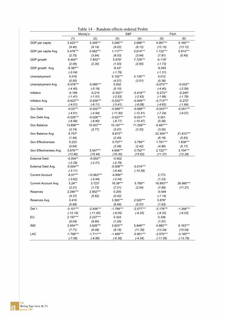
Table 14 – Random effects ordered Probit Moody’s S&P Fitch (1) (2) (3) (4) (5) (6)

GDP per capita 3.422*** 3.349*** 3.246*** 2.686*** 4.087*** 4.160*** (9.40) (9.14) (9.02) (8.12) (12.15) (13.12) GDP per capita Avg. 0.478*** 0.562*** 1.117*** 0.614*** 1.132*** 0.913*** (2.75) (3.84) (6.03) (3.94) (7.81) (5.45) GDP growth 6.464** 7.852** 5.979* 7.729*** -5.119* (2.06) (2.30) (1.93) (2.60) (-1.73) GDP growth Avg. -9.387** -8.43* -6.083 (-2.04) (-1.79) (-1.31) Unemployment 0.016 0.152*** 0.135*** 0.012 (0.50) (4.57) (3.01) (0.36) Unemployment Avg. -0.078*** -0.085*** 0.002 -0.073*** -0.033** (-4.40) (-5.18) (0.10) (-4.40) (-2.09) Inflation -0.199 -0.214 -0.353** -0.418*** -0.273** -0.245* (-1.41) (-1.51) (-2.53) (-2.93) (-1.96) (-1.79) Inflation Avg. -0.623*** -0.939*** -0.532*** -0.949*** -0.713*** -0.272* (-4.01) (-6.11) (-3.41) (-6.08) (-4.62) (-1.84) Gov Debt -0.03*** -0.032*** -0.085*** -0.088*** -0.043*** -0.051*** (-4.61) (-4.94) (-11.90) (-12.41) (-7.24) (-9.07) Gov Debt Avg. -0.026*** -0.028*** -0.027*** -0.031*** 0.001 (-6.99) (-8.80) (-8.77) (-10.47) (0.26) Gov Balance 13.898*** 10.937*** 10.187*** 11.559*** 9.487*** (3.74) (2.77) (3.07) (3.32) (3.00) Gov Balance Avg. 6.757* 8.873** 22.304*** 21.812*** (1.84) (2.40) (6.18) (5.83) Gov Effectiveness 0.223 0.707** 0.794** 1.761*** 1.838*** (0.64) (2.08) (2.42) (4.86) (5.17) Gov Effectiveness Avg. 3.679*** 3.547*** 4.606*** 3.752*** 2.722*** 3.104*** (13.46) (15.44) (16.30) (15.62) (11.37) (12.28) External Debt -0.004** -0.002** -0.002 (-2.29) (-2.21) (-0.79) External Debt Avg. -0.004*** -0.008*** -0.014*** (-3.11) (-6.40) (-10.39) Current Account -8.57*** -12.863*** -4.899** 2.772 (-3.62) (-5.94) (-2.04) (1.23) Current Account Avg. 5.24** 3.723* 18.39*** 5.769** 18.993*** 26.980*** (2.21) (1.73) (7.21) (2.54) (7.89) (11.27) Reserves 2.246*** 2.952*** 0.205 -0.549 (4.37) (5.82) (0.42) (-1.14) Reserves Avg. 0.416 3.365*** 2.520*** 0.876* (0.88) (6.94) (5.57) (1.83) Def 1 -3.101*** -2.936*** -1.789*** -2.077*** -2.176*** -1.266*** (-12.18) (-11.95) (-8.05) (-9.25) (-9.33) (-6.03) EU 2.197*** 2.237*** 0.324 0.336 (9.04) (8.90) (1.55) (1.57) IND 3.554*** 3.626*** 3.923*** 5.848*** 4.982*** 6.163*** (7.71) (9.08) (8.18) (11.38) (13.24) (15.54) LAC -1.766*** -1.711*** -1.485*** -0.901*** -2.570*** -3.165***

(-7.08) (-8.86) (-6.38) (-4.34) (-11.08) (-13.78)


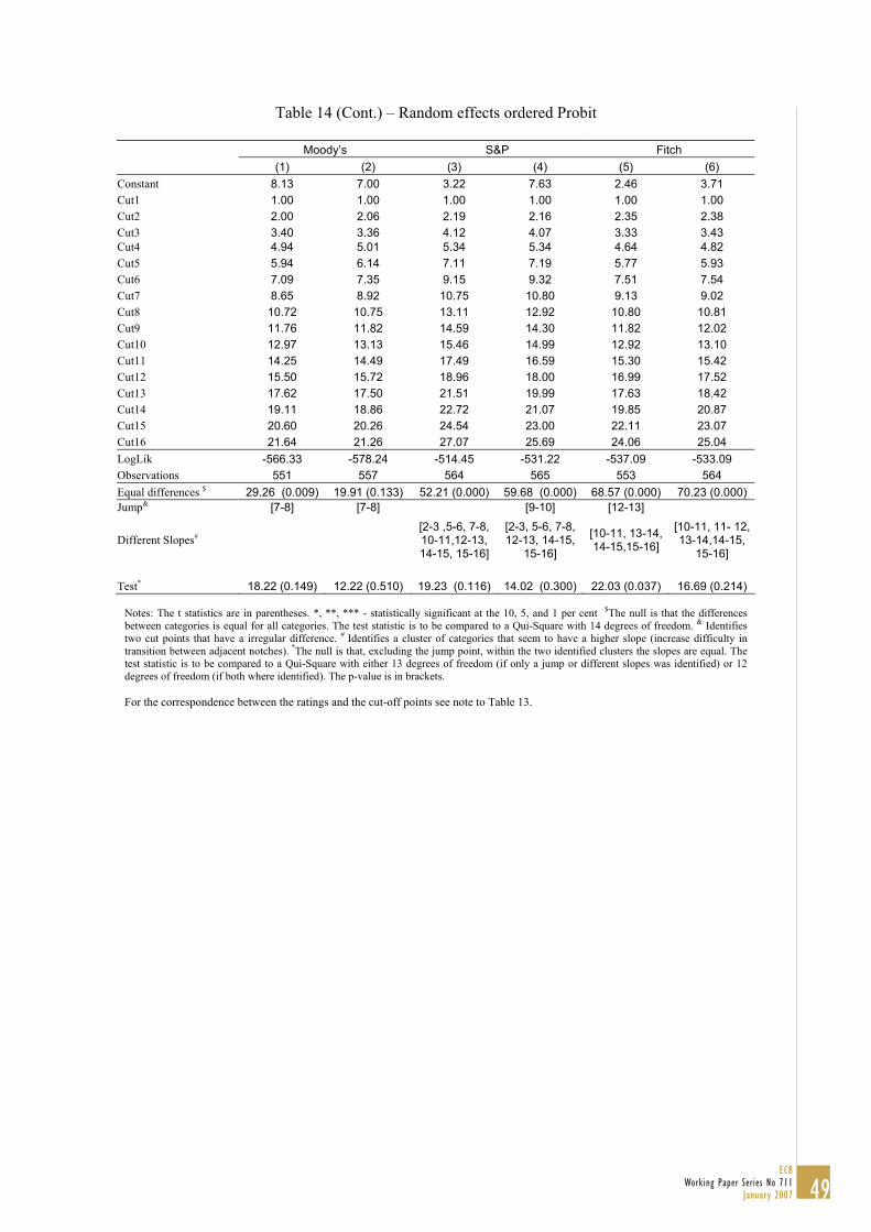
Table 14 (Cont.) – Random effects ordered Probit

Moody’s S&P Fitch (1) (2) (3) (4) (5) (6)

Constant 8.13 7.00 3.22 7.63 2.46 3.71 Cut1 1.00 1.00 1.00 1.00 1.00 1.00 Cut2 2.00 2.06 2.19 2.16 2.35 2.38 Cut3 3.40 3.36 4.12 4.07 3.33 3.43 Cut4 4.94 5.01 5.34 5.34 4.64 4.82 Cut5 5.94 6.14 7.11 7.19 5.77 5.93 Cut6 7.09 7.35 9.15 9.32 7.51 7.54 Cut7 8.65 8.92 10.75 10.80 9.13 9.02 Cut8 10.72 10.75 13.11 12.92 10.80 10.81 Cut9 11.76 11.82 14.59 14.30 11.82 12.02 Cut10 12.97 13.13 15.46 14.99 12.92 13.10 Cut11 14.25 14.49 17.49 16.59 15.30 15.42 Cut12 15.50 15.72 18.96 18.00 16.99 17.52 Cut13 17.62 17.50 21.51 19.99 17.63 18.42 Cut14 19.11 18.86 22.72 21.07 19.85 20.87 Cut15 20.60 20.26 24.54 23.00 22.11 23.07 Cut16 21.64 21.26 27.07 25.69 24.06 25.04 LogLik -566.33 -578.24 -514.45 -531.22 -537.09 -533.09 Observations 551 557 564 565 553 564 Equal differences $ 29.26 (0.009) 19.91 (0.133) 52.21 (0.000) 59.68 (0.000) 68.57 (0.000) 70.23 (0.000) Jump& [7-8] [7-8] [9-10] [12-13]

Different Slopes# [2-3 ,5-6, 7-8, 10-11,12-13, 14-15, 15-16]

[2-3, 5-6, 7-8, 12-13, 14-15,

15-16]

[10-11, 13-14, 14-15,15-16]

[10-11, 11- 12, 13-14,14-15,

15-16]

Test* 18.22 (0.149) 12.22 (0.510) 19.23 (0.116)

14.02 (0.300)

22.03 (0.037)

16.69 (0.214) Notes: The t statistics are in parentheses. *, **, *** - statistically significant at the 10, 5, and 1 per cent $The null is that the differences between categories is equal for all categories. The test statistic is to be compared to a Qui-Square with 14 degrees of freedom. & Identifies two cut points that have a irregular difference. # Identifies a cluster of categories that seem to have a higher slope (increase difficulty in transition between adjacent notches). *The null is that, excluding the jump point, within the two identified clusters the slopes are equal. The test statistic is to be compared to a Qui-Square with either 13 degrees of freedom (if only a jump or different slopes was identified) or 12 degrees of freedom (if both where identified). The p-value is in brackets. For the correspondence between the ratings and the cut-off points see note to Table 13.

49ECB


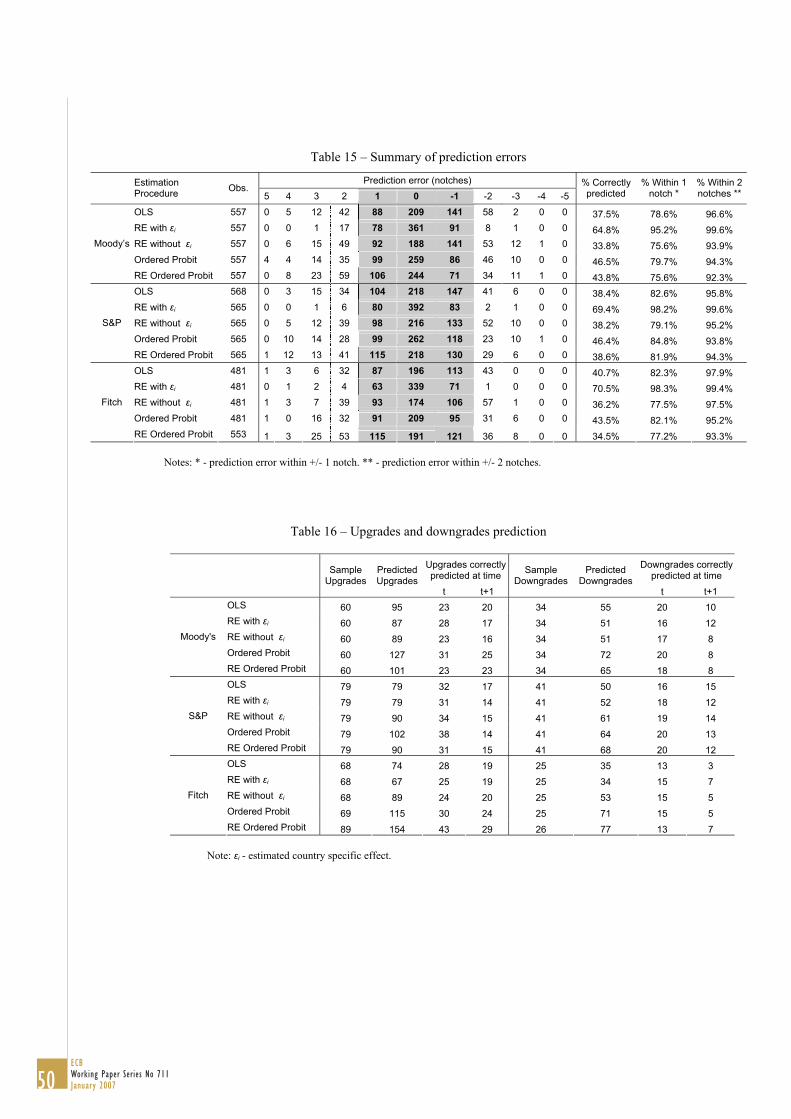
Table 15 – Summary of prediction errors

Notes: * - prediction error within +/- 1 notch. ** - prediction error within +/- 2 notches.

Table 16 – Upgrades and downgrades prediction

Upgrades correctly predicted at time

Downgrades correctly predicted at time

Sample

UpgradesPredicted Upgrades

t t+1

Sample Downgrades

Predicted Downgrades

t t+1 OLS 60 95 23 20 34 55 20 10 RE with εi 60 87 28 17 34 51 16 12 RE without εi 60 89 23 16 34 51 17 8 Ordered Probit 60 127 31 25 34 72 20 8

Moody's

RE Ordered Probit 60 101 23 23 34 65 18 8 OLS 79 79 32 17 41 50 16 15 RE with εi 79 79 31 14 41 52 18 12 RE without εi 79 90 34 15 41 61 19 14 Ordered Probit 79 102 38 14 41 64 20 13

S&P

RE Ordered Probit 79 90 31 15 41 68 20 12 OLS 68 74 28 19 25 35 13 3 RE with εi 68 67 25 19 25 34 15 7 RE without εi 68 89 24 20 25 53 15 5 Ordered Probit 69 115 30 24 25 71 15 5

Fitch

RE Ordered Probit 89 154 43 29 26 77 13 7

Note: εi - estimated country specific effect.

Prediction error (notches) Estimation

Procedure Obs. 5 4 3 2 1 0 -1 -2 -3 -4 -5

% Correctly predicted

% Within 1 notch *

% Within 2 notches **

OLS 557 0 5 12 42 88 209 141 58 2 0 0 37.5% 78.6% 96.6% RE with εi 557 0 0 1 17 78 361 91 8 1 0 0 64.8% 95.2% 99.6% RE without εi 557 0 6 15 49 92 188 141 53 12 1 0 33.8% 75.6% 93.9% Ordered Probit 557 4 4 14 35 99 259 86 46 10 0 0 46.5% 79.7% 94.3%

Moody’s

RE Ordered Probit 557 0 8 23 59 106 244 71 34 11 1 0 43.8% 75.6% 92.3% OLS 568 0 3 15 34 104 218 147 41 6 0 0 38.4% 82.6% 95.8% RE with εi 565 0 0 1 6 80 392 83 2 1 0 0 69.4% 98.2% 99.6% RE without εi 565 0 5 12 39 98 216 133 52 10 0 0 38.2% 79.1% 95.2% Ordered Probit 565 0 10 14 28 99 262 118 23 10 1 0 46.4% 84.8% 93.8%

S&P

RE Ordered Probit 565 1 12 13 41 115 218 130 29 6 0 0 38.6% 81.9% 94.3% OLS 481 1 3 6 32 87 196 113 43 0 0 0 40.7% 82.3% 97.9% RE with εi 481 0 1 2 4 63 339 71 1 0 0 0 70.5% 98.3% 99.4% RE without εi 481 1 3 7 39 93 174 106 57 1 0 0 36.2% 77.5% 97.5% Ordered Probit 481 1 0 16 32 91 209 95 31 6 0 0 43.5% 82.1% 95.2%

Fitch

RE Ordered Probit 553 1 3 25 53 115 191 121 36 8 0 0 34.5% 77.2% 93.3%


Table 17 – Example of country analysis: variables’ contribution to expected rating changes

17a – European countries Portugal Spain Greece Italy Ireland

1998 2005 1998 2005 1998 2005 1998 2005 1998 2005 Moody's Aa2 (15) Aa2 (15) Aa2 (15) Aaa (17) Baa1 (10) A1 (13) Aa3 (14) Aa2 (15) Aaa (17) Aaa (17) S&P AA (15) AA- (14) AA (15) AAA (17) BBB (9) A (12) AA (15) AA- (14) AA+ (16) AAA (17) R

atin

g$

Fitch AA (15) AA (15) AA (15) AAA (17) BBB (9) A (12) AA- (14) AA (15) AAA (17) AAA (17)

Macro contribution 0.53 0.73 0.93 1.69 1.98 2.28 1.33 1.52 1.70 0.91 1.08 1.26 1.46 1.83 2.20 Gov. contribution -0.69 -0.46 -0.23 0.27 0.65 1.03 -0.05 -0.01 0.02 -0.03 0.14 0.31 0.20 0.39 0.58 External contribution 0.09 0.12 0.15 0.22 0.31 0.39 0.18 0.24 0.31 0.17 0.24 0.30 0.15 0.21 0.26 European Union 0.00 0.00 0.00 0.00 0.00 0.00 0.00 0.00 0.00 0.00 0.00 0.00 0.00 0.00 0.00 M

oody

's

Overall change -0.07 0.39 0.86 2.19 2.95 3.70 1.46 1.75 2.03 1.05 1.46 1.87 1.81 2.43 3.05

Macro contribution 0.42 0.57 0.73 0.94 1.07 1.20 0.99 1.13 1.27 0.56 0.67 0.77 0.91 1.15 1.38 Gov. contribution -1.06 -0.88 -0.70 0.48 0.77 1.06 -0.13 -0.10 -0.08 0.07 0.21 0.34 0.83 0.98 1.14 External contribution 0.03 0.05 0.08 0.07 0.14 0.21 0.06 0.11 0.16 0.05 0.11 0.16 0.05 0.09 0.14 European Union 0.00 0.00 0.00 0.00 0.00 0.00 0.00 0.00 0.00 0.00 0.00 0.00 0.00 0.00 0.00

S&P

Overall change -0.61 -0.25 0.11 1.49 1.98 2.47 0.91 1.14 1.36 0.69 0.98 1.26 1.78 2.22 2.66

Macro contribution 0.90 0.99 1.08 1.78 2.01 2.25 1.43 1.56 1.69 1.06 1.18 1.30 1.92 2.14 2.35 Gov. contribution -1.26 -1.05 -0.85 -0.46 -0.13 0.19 -0.11 -0.08 -0.06 -0.45 -0.29 -0.14 0.15 0.31 0.47 External contribution -0.06 -0.03 -0.01 -0.16 -0.09 -0.02 -0.13 -0.07 -0.01 -0.12 -0.07 -0.01 -0.11 -0.06 -0.01European Union 0.00 0.00 0.00 0.00 0.00 0.00 0.00 0.00 0.00 0.00 0.00 0.00 0.00 0.00 0.00

Fitc

h

Overall change -0.42 -0.10 0.23 1.16 1.79 2.42 1.19 1.40 1.62 0.49 0.81 1.14 1.97 2.39 2.81

17b – European countries Czech Republic Hungary Poland Slovakia Slovenia

1998 2005 1998 2005 1998 2005 1998 2005 1998 2005 Moody's Baa1 (10) A1 (13) Baa3 (10) A1 (13) Baa3 (10) A2 (12) Ba1 (7) A2 (12) A3 (11) Aa3 (14) S&P A- (11) A- (11) BBB (9) A- (11) BBB- (8) BBB+ (10) BB+ (7) A (12) A (12) AA- (14) R

atin

g$

Fitch BBB+ (10) A (12) BBB (9) BBB+ (10) BBB+ (10) BBB+ (10) BB+(7) A (12) A- (11) AA- (14)

Macro contribution 1.43 1.76 2.08 2.08 2.36 2.65 0.59 0.90 1.21 1.30 1.57 1.84 1.07 1.22 1.38 Gov. contribution -0.75 -0.59 -0.43 -0.39 -0.29 -0.19 -0.61 -0.42 -0.23 -0.32 -0.11 0.10 -0.23 -0.10 0.02 External contribution -0.08 -0.05 -0.01 0.00 0.09 0.17 -0.34 -0.23 -0.13 -0.04 0.26 0.56 0.13 0.17 0.22 European Union 1.42 1.60 1.77 1.42 1.60 1.77 1.42 1.60 1.77 1.42 1.60 1.77 1.42 1.60 1.77 M

oody

's

Overall change 2.03 2.72 3.41 3.11 3.76 4.41 1.06 1.85 2.63 2.37 3.32 4.28 2.39 2.89 3.39

Macro contribution 1.24 1.46 1.68 1.48 1.69 1.89 0.86 1.03 1.19 1.23 1.39 1.55 0.76 0.87 0.99 Gov. contribution -1.05 -0.93 -0.80 -0.25 -0.18 -0.11 -0.63 -0.49 -0.35 -0.45 -0.28 -0.11 -0.18 -0.08 0.02 External contribution -0.02 0.00 0.03 0.02 0.08 0.15 -0.09 -0.01 0.07 -0.28 -0.02 0.23 0.01 0.04 0.07 European Union 0.07 0.19 0.31 0.07 0.19 0.31 0.07 0.19 0.31 0.07 0.19 0.31 0.07 0.19 0.31

S&P

Overall change 0.23 0.73 1.22 1.31 1.77 2.24 0.20 0.72 1.23 0.58 1.28 1.97 0.66 1.02 1.38

Macro contribution 1.53 1.73 1.92 2.24 2.48 2.71 0.95 1.17 1.39 1.51 1.73 1.95 1.20 1.32 1.44 Gov. contribution -0.80 -0.67 -0.54 -0.35 -0.27 -0.19 -0.88 -0.72 -0.55 0.20 0.38 0.57 0.13 0.24 0.35 External contribution 0.05 0.10 0.15 -0.10 -0.02 0.05 0.11 0.24 0.38 0.27 0.73 1.19 -0.08 -0.04 -0.01European Union 0.08 0.22 0.36 0.08 0.22 0.36 0.08 0.22 0.36 0.08 0.22 0.36 0.08 0.22 0.36

Fitc

h

Overall change 0.86 1.37 1.89 1.88 2.40 2.93 0.26 0.92 1.58 2.06 3.06 4.07 1.33 1.73 2.14 Notes: The block contributions were calculated using the changes in the variables multiplied by the short-run coefficients estimated by random effects ordered probit, and then aggregated. The only exception was unemployment, for which we used the long-run coefficient. The upper and lower bounds where calculated using plus and minus one standard deviation. $ The quantitative rating scale is in brackets.

51ECB


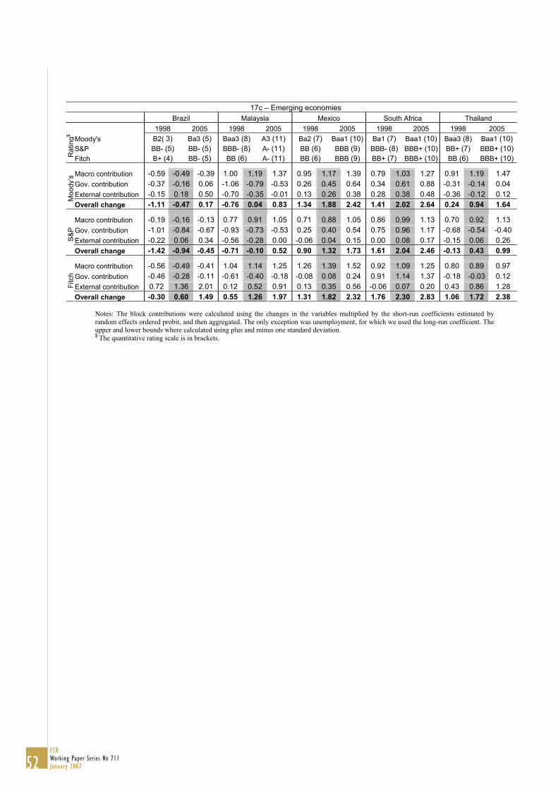
17c – Emerging economies Brazil Malaysia Mexico South Africa Thailand

1998 2005 1998 2005 1998 2005 1998 2005 1998 2005 Moody's B2( 3) Ba3 (5) Baa3 (8) A3 (11) Ba2 (7) Baa1 (10) Ba1 (7) Baa1 (10) Baa3 (8) Baa1 (10) S&P BB- (5) BB- (5) BBB- (8) A- (11) BB (6) BBB (9) BBB- (8) BBB+ (10) BB+ (7) BBB+ (10)

Rat

ing$

Fitch B+ (4) BB- (5) BB (6) A- (11) BB (6) BBB (9) BB+ (7) BBB+ (10) BB (6) BBB+ (10)

Macro contribution -0.59 -0.49 -0.39 1.00 1.19 1.37 0.95 1.17 1.39 0.79 1.03 1.27 0.91 1.19 1.47 Gov. contribution -0.37 -0.16 0.06 -1.06 -0.79 -0.53 0.26 0.45 0.64 0.34 0.61 0.88 -0.31 -0.14 0.04 External contribution -0.15 0.18 0.50 -0.70 -0.35 -0.01 0.13 0.26 0.38 0.28 0.38 0.48 -0.36 -0.12 0.12

Moo

dy’s

Overall change -1.11 -0.47 0.17 -0.76 0.04 0.83 1.34 1.88 2.42 1.41 2.02 2.64 0.24 0.94 1.64

Macro contribution -0.19 -0.16 -0.13 0.77 0.91 1.05 0.71 0.88 1.05 0.86 0.99 1.13 0.70 0.92 1.13 Gov. contribution -1.01 -0.84 -0.67 -0.93 -0.73 -0.53 0.25 0.40 0.54 0.75 0.96 1.17 -0.68 -0.54 -0.40 External contribution -0.22 0.06 0.34 -0.56 -0.28 0.00 -0.06 0.04 0.15 0.00 0.08 0.17 -0.15 0.06 0.26 S&

P

Overall change -1.42 -0.94 -0.45 -0.71 -0.10 0.52 0.90 1.32 1.73 1.61 2.04 2.46 -0.13 0.43 0.99

Macro contribution -0.56 -0.49 -0.41 1.04 1.14 1.25 1.26 1.39 1.52 0.92 1.09 1.25 0.80 0.89 0.97 Gov. contribution -0.46 -0.28 -0.11 -0.61 -0.40 -0.18 -0.08 0.08 0.24 0.91 1.14 1.37 -0.18 -0.03 0.12 External contribution 0.72 1.36 2.01 0.12 0.52 0.91 0.13 0.35 0.56 -0.06 0.07 0.20 0.43 0.86 1.28 Fi

tch

Overall change -0.30 0.60 1.49 0.55 1.26 1.97 1.31 1.82 2.32 1.76 2.30 2.83 1.06 1.72 2.38 Notes: The block contributions were calculated using the changes in the variables multiplied by the short-run coefficients estimated by random effects ordered probit, and then aggregated. The only exception was unemployment, for which we used the long-run coefficient. The upper and lower bounds where calculated using plus and minus one standard deviation. $ The quantitative rating scale is in brackets.


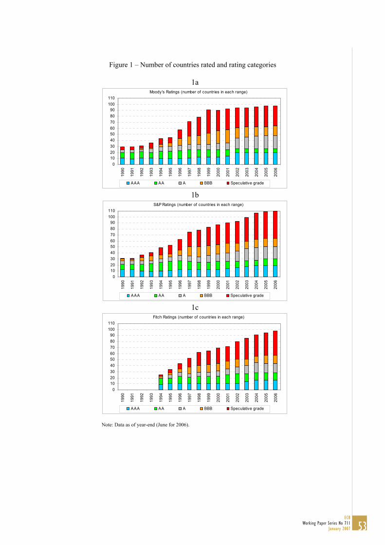
Figure 1 – Number of countries rated and rating categories 1a

Moody's Ratings (number of countries in each range)

0102030405060708090

100110

1990

1991

1992

1993

1994

1995

1996

1997

1998

1999

2000

2001

2002

2003

2004

2005

2006

AAA AA A BBB Speculative grade

1b S&P Ratings (number of countries in each range)

0102030405060708090

100110

1990

1991

1992

1993

1994

1995

1996

1997

1998

1999

2000

2001

2002

2003

2004

2005

2006


1c Fitch Ratings (number of countries in each range)

0102030405060708090

100110

1990

1991

1992

1993

1994

1995

1996

1997

1998

1999

2000

2001

2002

2003

2004

2005

2006


Note: Data as of year-end (June for 2006).

53ECB


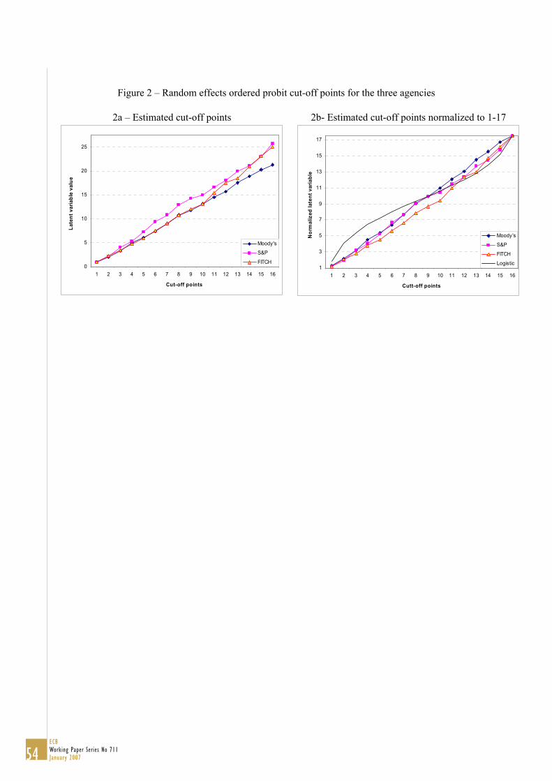
Figure 2 – Random effects ordered probit cut-off points for the three agencies

2a – Estimated cut-off points 2b- Estimated cut-off points normalized to 1-17

0

5

10

15

20

25

1 2 3 4 5 6 7 8 9 10 11 12 13 14 15 16

Cut-off points

Late

nt v

aria

ble

valu

e

Moody's

S&P

FITCH1

3

5

7

9

11

13

15

17

1 2 3 4 5 6 7 8 9 10 11 12 13 14 15 16

Cutt-off points

Nor

mal

ized

late

nt v

aria

ble

Moody's

S&P

FITCH

Logistic


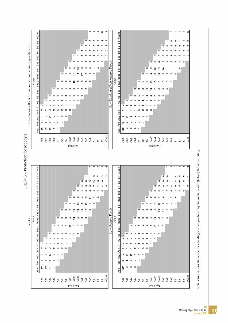
Figu

re 3

– P

redi

ctio

n fo

r Moo

dy’s

3a

– O

LS

3b –

Ran

dom

eff

ects

est

imat

ion

with

out c

ount

ry sp

ecifi

c er

ror

Aaa

Aa1

Aa2

Aa3

A1A

2A

3B

aa1

Baa

2B

aa3

Ba1

Ba2

Ba3

B1B2

B3≤C

aa1

Aaa

866

00

0Aa

150

63

60

0Aa

211

1122

22

04

Aa3

13

30

02

30

A10

16

53

13

0A2

00

40

00

00

A30

22

21

00

0Ba

a10

82

115

20

0Ba

a20

89

1310

70

0Ba

a31

05

1913

30

0Ba

10

314

84

14

0Ba

20

1210

36

50

1Ba

30

111

88

31

0B1

02

37

135

1B2

02

25

75

B30

46

37

≤Caa

10

13

11

Actu

alPredicted

Aaa

Aa1

Aa2

Aa3

A1

A2

A3

Baa

1Ba

a2Ba

a3B

a1Ba

2B

a3B

1B2

B3≤C

aa1

Aaa

866

10

0Aa

140

83

60

0Aa

216

821

22

04

Aa3

50

30

43

21

A11

41

60

22

20

A20

00

51

20

00

A30

02

30

50

00

Baa1

00

61

65

12

0Ba

a20

09

913

125

10

Baa3

01

15

813

30

0Ba

10

03

279

51

40

Ba2

00

89

67

81

1Ba

30

10

44

75

30

B10

14

75

66

0B2

00

16

93

6B3

00

05

410

≤Caa

10

02

38

Actu

al

Predicted

3c

– O

rder

ed P

robi

t 3d

– R

ando

m e

ffec

ts o

rder

ed P

robi

t

Aaa

Aa1

Aa2

Aa3

A1A

2A

3B

aa1

Baa

2B

aa3

Ba1

Ba2

Ba3

B1B2

B3≤C

aa1

Aaa

139

152

60

0Aa

13

114

11

04

Aa2

36

111

10

00

Aa3

32

10

22

00

0A1

21

14

14

10

0A2

05

42

12

00

0A3

01

41

20

00

0Ba

a10

62

95

41

00

Baa2

06

1013

53

00

0Ba

a33

06

2517

20

30

Ba1

02

218

61

40

0Ba

20

25

17

30

00

Ba3

04

76

42

11

B11

62

108

40

B21

45

105

4B3

01

56

6≤C

aa1

03

413

Actu

al

Predicted

Aaa

Aa1

Aa2

Aa3

A1A2

A3Ba

a1Ba

a2Ba

a3Ba

1B

a2Ba

3B1

B2

B3

≤Caa

1A

aa13

915

56

0A

a13

714

11

0A

a20

08

11

04

Aa3

52

21

43

00

A1

12

05

64

53

0A

20

00

14

10

00

A3

00

03

09

01

0B

aa1

00

14

1015

43

0B

aa2

00

72

58

1 00

0B

aa3

00

06

189

40

3B

a10

00

1914

57

40

Ba2

00

51

32

50

1B

a30

21

51

55

40

B1

01

55

66

61

B2

01

54

61

3B

30

03

63

7≤C

aa1

00

55

13

Act

ual

Predicted

N

ote:

obs

erva

tions

abo

ve (b

elow

) the

dia

gona

l are

pre

dict

ed b

y th

e m

odel

abo

ve (b

elow

) the

act

ual r

atin

g.

55ECB


Figu

re 4

– P

redi

ctio

n fo

r S&

P 4a

– O

LS

4b –

Ran

dom

eff

ects

est

imat

ion

with

out c

ount

ry sp

ecifi

c er

ror

AAA

AA+

AA

AA-

A+

AA-

BB

B+B

BB

BBB

-BB

+BB

BB-

B+B

B-<C

CC

+A

AA

6716

01

1A

A+

3526

70

60

AA

1512

111

20

0A

A-

30

14

25

00

A+

07

42

62

00

A1

01

12

01

2A

-0

01

121

00

0B

BB+

03

116

21

00

BB

B0

34

1112

20

0B

BB-

03

1821

90

00

BB

+0

116

715

80

0B

B0

115

194

03

0B

B-

04

138

76

10

B+

00

79

122

3B

00

35

46

B-

24

35

4≤C

CC

+0

03

4

Act

ual

Predicted

AAA

AA+

AAA

A-A

+A

A-

BBB

+BB

BB

BB-

BB+

BB

BB-

B+B

B-

<CC

C+

AAA

7015

01

2A

A+31

2910

05

0A

A16

64

03

00

AA-

34

43

28

00

A+

04

21

32

01

A5

40

13

00

2A

-0

11

60

00

0B

BB+

02

103

11

00

BBB

16

1016

111

00

BBB

-0

113

219

10

0B

B+0

216

917

80

0B

B0

214

194

04

0B

B-0

48

67

61

0B

+0

29

1010

21

B0

13

73

7B

-1

32

53

≤CC

C+

00

46

Act

ual

Predicted

4c

– O

rder

ed P

robi

t 4d

– R

ando

m e

ffec

ts o

rder

ed P

robi

t

AAA

AA

+AA

AA-

A+A

A-

BBB

+B

BBB

BB-

BB

+BB

BB-

B+B

B-<C

CC

+AA

A96

261

16

AA+

2121

131

21

AA2

74

21

30

AA-

10

00

10

00

A+0

03

23

40

00

A0

54

14

40

10

A-1

00

213

20

30

BBB+

00

25

42

00

0BB

B0

05

612

30

00

BBB-

00

217

359

00

0BB

+0

01

1211

158

02

BB0

00

1520

52

20

BB-

00

212

94

62

1B+

00

05

105

10

B0

00

311

38

B-0

22

32

1≤C

CC

+0

20

77

Actu

al

Predicted

AAA

AA+

AAA

A-A

+A

A-

BBB

+BB

BB

BB-

BB+

BB

BB-

B+B

B-

<CC

C+

AAA

8332

31

70

AA+

3519

100

30

0A

A2

35

32

50

0A

A-0

06

20

40

00

A+

03

21

22

01

1A

02

12

30

01

0A

-0

03

131

21

00

BBB

+0

02

12

00

00

BBB

06

109

1 01

00

0B

BB-

12

1927

131

00

0B

B+0

011

613

80

20

BB

02

1221

42

20

0B

B-0

511

96

70

1B

+0

11

49

31

B0

58

84

6B

-2

00

23

≤CC

C+

31

66

Act

ual

Predicted

N

ote:

obs

erva

tions

abo

ve (b

elow

) the

dia

gona

l are

pre

dict

ed b

y th

e m

odel

abo

ve (b

elow

) the

act

ual r

atin

g.


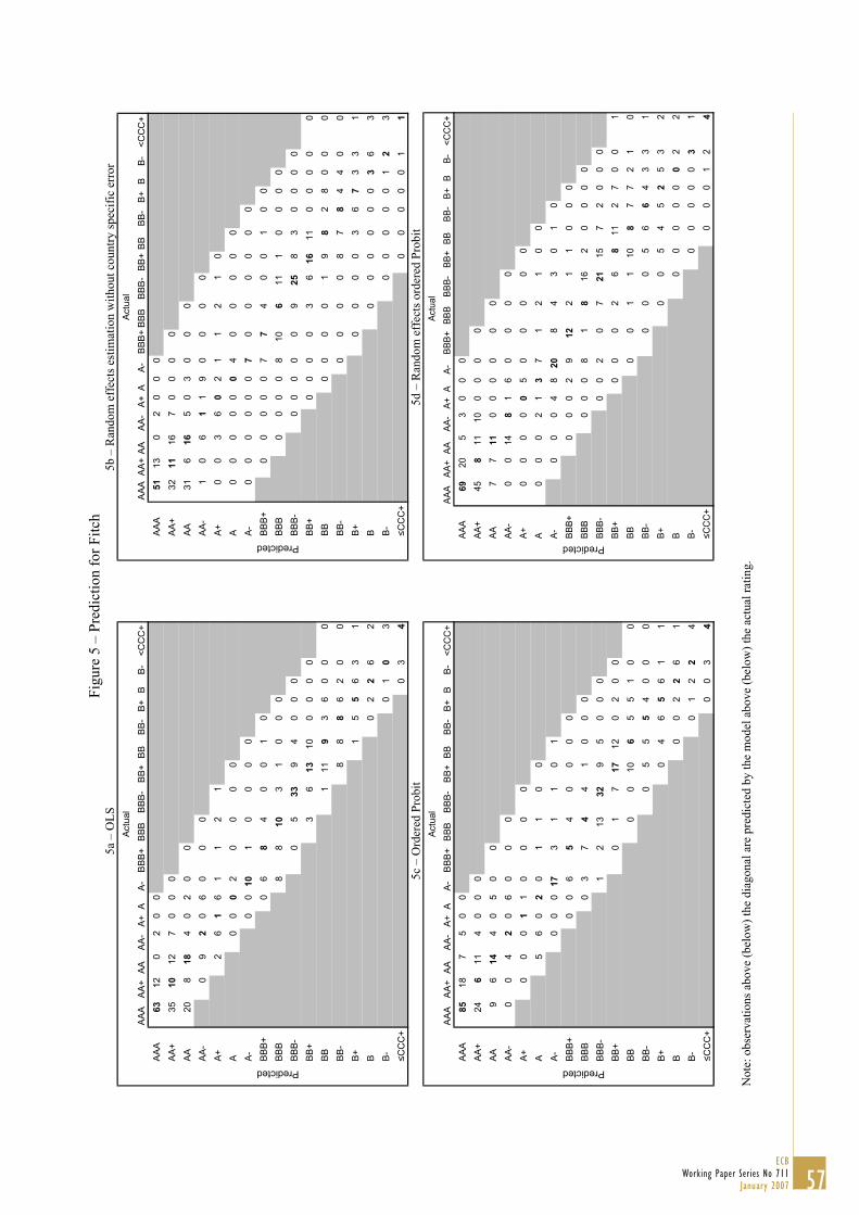
Figu

re 5

– P

redi

ctio

n fo

r Fitc

h 5a

– O

LS

5b –

Ran

dom

eff

ects

est

imat

ion

with

out c

ount

ry sp

ecifi

c er

ror

AAA

AA

+AA

AA-

A+A

A-

BBB

+B

BBB

BB-

BB

+BB

BB-

B+B

B-<C

CC

+AA

A63

120

20

0AA

+35

1012

70

00

AA20

818

40

20

0AA

-0

92

06

00

0A+

26

16

11

21

A0

00

20

00

0A-

00

101

00

00

BBB+

06

84

00

10

BBB

88

103

10

00

BBB-

05

339

40

00

BB+

36

1310

00

00

BB1

119

36

00

0BB

-8

88

62

00

B+1

55

63

1B

02

26

2B-

01

03

≤CC

C+

03

4

Actu

alPredicted

AAA

AA+

AAA

A-A

+A

A-

BBB

+BB

BB

BB-

BB+

BB

BB-

B+B

B-

<CC

C+

AAA

5113

02

00

0A

A+32

1116

70

00

0A

A31

616

50

30

00

AA-

10

61

19

00

00

A+

00

36

02

11

21

0A

00

00

00

40

00

00

A-

00

00

00

70

00

00

0B

BB+

00

00

07

74

00

10

0B

BB0

00

08

106

111

00

00

BBB

-0

00

00

925

83

00

00

BB+

00

00

36

1611

00

00

0B

B0

00

01

98

28

00

0B

B-0

00

08

78

44

00

B+

00

00

36

73

31

B0

00

00

03

63

B-

00

00

01

23

≤CC

C+

00

00

01

1

Act

ual

Predicted

5c

– O

rder

ed P

robi

t 5d

– R

ando

m e

ffec

ts o

rder

ed P

robi

t

AAA

AA

+AA

AA-

A+A

A-

BBB

+B

BBB

BB-

BB

+BB

BB-

B+B

B-<C

CC

+AA

A85

187

50

0AA

+24

611

40

00

AA9

614

40

50

0AA

-0

04

20

60

00

A+0

00

11

00

00

A5

60

20

11

00

A-0

00

173

11

01

BBB+

00

65

40

00

0BB

B0

37

44

10

00

BBB-

12

1332

95

00

0BB

+0

17

1712

02

00

BB0

010

65

51

00

BB-

05

55

40

00

B+0

46

56

11

B0

02

26

1B-

01

22

4≤C

CC

+0

03

4

Actu

al

Predicted

AAA

AA+

AAAA

-A+

AA-

BBB+

BBB

BBB-

BB+

BBBB

-B+

BB-

<CC

C+

AAA

6920

53

00

0AA

+45

811

100

00

0AA

77

110

00

00

0AA

-0

014

81

60

00

0A+

00

00

05

00

00

0A

00

02

13

71

21

00

A-0

00

48

208

43

01

0BB

B+0

00

29

122

11

00

0BB

B0

00

81

816

20

00

0BB

B-0

02

07

2115

72

00

0BB

+0

00

26

811

27

00

1BB

00

11

108

77

21

0BB

-0

00

56

64

33

1B +

00

54

52

53

2B

00

00

00

22

B-0

00

00

31

≤CC

C+

00

01

24

Actu

al

Predicted

N

ote:

obs

erva

tions

abo

ve (b

elow

) the

dia

gona

l are

pre

dict

ed b

y th

e m

odel

abo

ve (b

elow

) the

act

ual r

atin

g.

57ECB


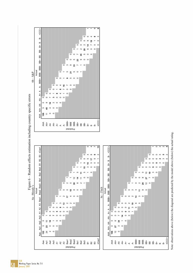
Fi

gure

6 –

Ran

dom

eff

ects

est

imat

ion

incl

udin

g co

untry

spec

ific

erro

rs

6a –

Moo

dy’s

6b

– S

&P

Aaa

Aa1

Aa2

Aa3

A1A

2A

3B

aa1

Baa

2B

aa3

Ba1

Ba2

Ba3

B1B2

B3≤C

aa1

Aaa

122

30

0Aa

124

2310

10

Aa2

20

186

00

Aa3

00

17

20

0A1

00

05

01

0A2

00

68

31

0A3

00

713

20

0Ba

a10

02

170

21

Baa2

02

418

51

0Ba

a30

08

3912

10

Ba1

00

814

51

0Ba

20

211

111

10

Ba3

10

515

90

0B1

01

315

54

0B2

00

517

84

B30

05

67

≤Caa

10

12

13

Actu

al

Predicted

AAA

AA+

AA

AA-

A+

AA-

BBB+

BBB

BB

B-BB

+B

BB

B-

B+B

B-<C

CC

+A

AA

109

50

0A

A+

1145

90

0A

A0

416

70

0A

A-

00

23

10

0A

+0

00

81

00

A0

04

84

00

A-

01

716

11

0B

BB+

00

78

53

0B

BB

00

521

90

0B

BB-

00

533

50

0B

B+

00

723

71

0B

B1

19

352

00

BB

-0

05

202

00

B+

00

614

90

1B

00

719

41

B-

00

18

9≤C

CC

+0

03

6

Act

ual

Predicted

6c

– F

itch

AAA

AA

+AA

AA-

A+A

A-

BBB

+B

BBB

BB-

BB

+BB

BB-

B+B

B-<C

CC

+AA

A10

60

00

0AA

+12

276

00

0AA

03

347

00

0AA

-0

114

00

00

A+0

00

00

00

A0

011

20

00

A-1

319

22

10

BBB+

06

133

00

0BB

B0

311

20

10

BBB-

08

298

00

0BB

+0

1227

100

00

BB0

719

20

00

BB-

03

98

00

1B+

05

86

00

B0

32

52

B-0

35

2≤C

CC

+0

25

Actu

al

Predicted

Not

e: o

bser

vatio

ns a

bove

(bel

ow) t

he d

iago

nal a

re p

redi

cted

by

the

mod

el a

bove

(bel

ow) t

he a

ctua

l rat

ing.


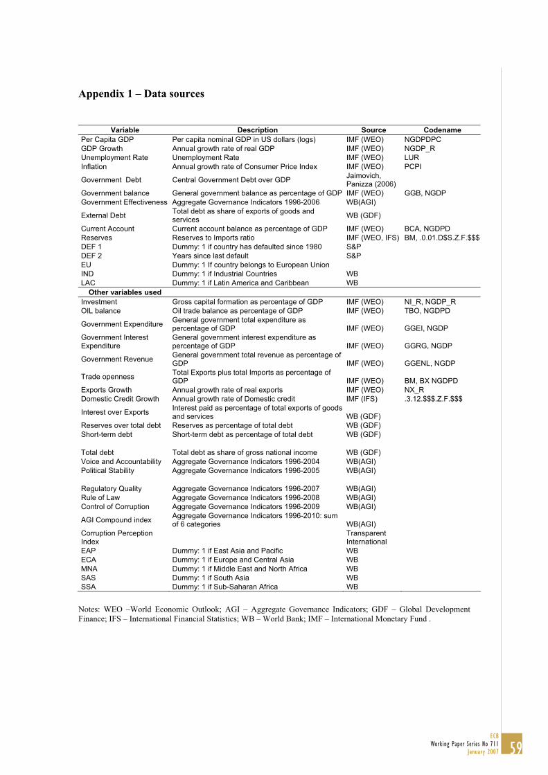
Appendix 1 – Data sources

Variable Description Source Codename

Per Capita GDP Per capita nominal GDP in US dollars (logs) IMF (WEO) NGDPDPC GDP Growth Annual growth rate of real GDP IMF (WEO) NGDP_R Unemployment Rate Unemployment Rate IMF (WEO) LUR Inflation Annual growth rate of Consumer Price Index IMF (WEO) PCPI

Government Debt Central Government Debt over GDP Jaimovich, Panizza (2006)

Government balance General government balance as percentage of GDP IMF (WEO) GGB, NGDP Government Effectiveness Aggregate Governance Indicators 1996-2006 WB(AGI)

External Debt Total debt as share of exports of goods and services WB (GDF)

Current Account Current account balance as percentage of GDP IMF (WEO) BCA, NGDPD Reserves Reserves to Imports ratio IMF (WEO, IFS) BM, .0.01.D$S.Z.F.$$$DEF 1 Dummy: 1 if country has defaulted since 1980 S&P DEF 2 Years since last default S&P EU Dummy: 1 If country belongs to European Union IND Dummy: 1 if Industrial Countries WB LAC Dummy: 1 if Latin America and Caribbean WB

Other variables used Investment Gross capital formation as percentage of GDP IMF (WEO) NI_R, NGDP_R OIL balance Oil trade balance as percentage of GDP IMF (WEO) TBO, NGDPD

Government Expenditure General government total expenditure as percentage of GDP IMF (WEO) GGEI, NGDP

Government Interest Expenditure

General government interest expenditure as percentage of GDP IMF (WEO) GGRG, NGDP

Government Revenue General government total revenue as percentage of GDP IMF (WEO) GGENL, NGDP

Trade openness Total Exports plus total Imports as percentage of GDP IMF (WEO) BM, BX NGDPD

Exports Growth Annual growth rate of real exports IMF (WEO) NX_R Domestic Credit Growth Annual growth rate of Domestic credit IMF (IFS) .3.12.$$$.Z.F.$$$

Interest over Exports Interest paid as percentage of total exports of goods and services WB (GDF)

Reserves over total debt Reserves as percentage of total debt WB (GDF) Short-term debt Short-term debt as percentage of total debt WB (GDF) Total debt Total debt as share of gross national income WB (GDF) Voice and Accountability Aggregate Governance Indicators 1996-2004 WB(AGI) Political Stability Aggregate Governance Indicators 1996-2005 WB(AGI) Regulatory Quality Aggregate Governance Indicators 1996-2007 WB(AGI) Rule of Law Aggregate Governance Indicators 1996-2008 WB(AGI) Control of Corruption Aggregate Governance Indicators 1996-2009 WB(AGI)

AGI Compound index Aggregate Governance Indicators 1996-2010: sum of 6 categories WB(AGI)

Corruption Perception Index

Transparent International

EAP Dummy: 1 if East Asia and Pacific WB ECA Dummy: 1 if Europe and Central Asia WB MNA Dummy: 1 if Middle East and North Africa WB SAS Dummy: 1 if South Asia WB SSA Dummy: 1 if Sub-Saharan Africa WB Notes: WEO –World Economic Outlook; AGI – Aggregate Governance Indicators; GDF – Global Development Finance; IFS – International Financial Statistics; WB – World Bank; IMF – International Monetary Fund .

59ECB


Appendix 2 – Countries and years in most extensive rating sample

Country Years Obs. Country Years Obs. Country Years Obs.

Andorra 4 4 Greece 19 42 Nicaragua 9 9 Argentina 21 45 Grenada 5 5 Nigeria 1 2 Aruba 5 5 Guatemala 10 17 Norway 32 73 Australia 36 79 Honduras 8 8 Oman 11 21 Austria 32 75 Hong Kong 21 56 Pakistan 13 26 Azerbaijan 7 7 Hungary 15 34 Panama 10 29 Bahamas 10 14 Iceland 18 43 Papua New Guinea 9 25 Bahrain 11 23 India 17 32 Paraguay 11 20 Barbados 12 20 Indonesia 15 38 Peru 10 26 Belgium 19 51 Iran 5 5 Philippines 14 36 Belize 8 15 Ireland 20 52 Poland 12 36 Benin 4 7 Isle of Man 7 7 Portugal 21 53 Bermuda 13 38 Israel 19 43 Qatar 11 19 Bolivia 9 21 Italy 21 53 Romania 11 32 Bosnia and Herzegovina 3 3 Jamaica 8 13 Russia 11 33

Botswana 6 12 Japan 31 70 San Marino 6 6 Brazil 21 47 Jordan 12 23 Saudi Arabia 11 18 Bulgaria 11 29 Kazakhstan 11 33 Senegal 7 7 Burkina Faso 3 3 Korea 19 39 Serbia 3 5 Cameroon 4 8 Kuwait 12 33 Singapore 18 45 Canada 36 85 Latvia 10 27 Slovakia 13 33 Cape Verde 4 4 Lebanon 10 30 Slovenia 11 33 Chile 15 36 Lesotho 5 5 South Africa 13 39 China 19 43 Liechtenstein 11 11 Spain 19 51 Colombia 14 41 Lithuania 11 31 Sri Lanka 2 4 Cook Islands 10 10 Luxembourg 18 44 Suriname 8 14 Costa Rica 10 29 Macao 10 10 Sweden 30 61 Croatia 10 30 Macedonia 3 5 Switzerland 26 58 Cuba 8 8 Madagascar 3 3 Taiwan 18 37 Cyprus 13 27 Malawi 4 4 Thailand 18 45 Czech Republic 14 40 Malaysia 21 48 Trinidad and Tobago 14 25 Denmark 36 75 Mali 3 6 Tunisia 12 22 Dominican Republic 10 22 Malta 13 37 Turkey 15 43

Egypt 10 26 Mauritius 11 11 Turkmenistan 10 10 El Salvador 11 32 Mexico 17 44 Uganda 2 2 Ecuador 10 22 Moldova 10 19 Ukraine 9 21 Estonia 10 25 Mongolia 8 10 United Arab Emirates 11 11 Fiji Islands 8 8 Montenegro 3 3 United Kingdom 29 71 Finland 30 73 Montserrat 3 3 United States of America 37 86 France 32 60 Morocco 9 17 Uruguay 14 39 Gambia 5 5 Mozambique 4 7 Venezuela 30 60 Georgia 2 2 Namibia 2 2 Vietnam 5 12 Germany 24 58 Netherlands 21 52 Ghana 4 8 New Zealand 37 73 Note: For instance, for 2005 the total number of rated countries was 130 (Fitch, 98; S&P, 110; Moody's, 98). Countries with 3 ratings: 78.


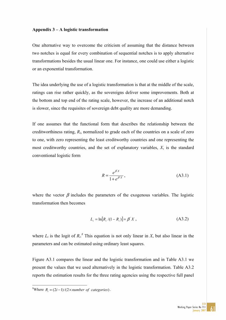
Appendix 3 – A logistic transformation

One alternative way to overcome the criticism of assuming that the distance between

two notches is equal for every combination of sequential notches is to apply alternative

transformations besides the usual linear one. For instance, one could use either a logistic

or an exponential transformation.

The idea underlying the use of a logistic transformation is that at the middle of the scale,

ratings can rise rather quickly, as the sovereigns deliver some improvements. Both at

the bottom and top end of the rating scale, however, the increase of an additional notch

is slower, since the requisites of sovereign debt quality are more demanding.

If one assumes that the functional form that describes the relationship between the

creditworthiness rating, Ri, normalized to grade each of the countries on a scale of zero

to one, with zero representing the least creditworthy countries and one representing the

most creditworthy countries, and the set of explanatory variables, X, is the standard

conventional logistic form

X

X

eeR '1

'

β

β

+= , (A3.1)

where the vector β includes the parameters of the exogenous variables. The logistic

transformation then becomes

[ ] XRRL iii')1/(ln β=−= , (A3.2)

where Li is the logit of Ri.8 This equation is not only linear in X, but also linear in the

parameters and can be estimated using ordinary least squares.

Figure A3.1 compares the linear and the logistic transformation and in Table A3.1 we

present the values that we used alternatively in the logistic transformation. Table A3.2

reports the estimation results for the three rating agencies using the respective full panel

8Where (2 1) /(2 )iR i number of categories= − × .

61ECB


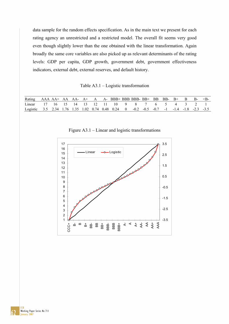
data sample for the random effects specification. As in the main text we present for each

rating agency an unrestricted and a restricted model. The overall fit seems very good

even though slightly lower than the one obtained with the linear transformation. Again

broadly the same core variables are also picked up as relevant determinants of the rating

levels: GDP per capita, GDP growth, government debt, government effectiveness

indicators, external debt, external reserves, and default history.

Table A3.1 – Logistic transformation

Rating AAA AA+ AA AA- A+ A A- BBB+ BBB BBB- BB+ BB BB- B+ B B- <B- Linear 17 16 15 14 13 12 11 10 9 8 7 6 5 4 3 2 1 Logistic 3.5 2.34 1.76 1.35 1.02 0.74 0.48 0.24 0 -0.2 -0.5 -0.7 -1 -1.4 -1.8 -2.3 -3.5

Figure A3.1 – Linear and logistic transformations

123456789

1011121314151617

CC

C+ B- B B+ B

B-

BB

BB+

BB

B-

BB

B

BBB

+ A- A A+

AA

-

AA

AA

+

AA

A

-3.5

-2.5

-1.5

-0.5

0.5

1.5

2.5

3.5

Linear Logistic


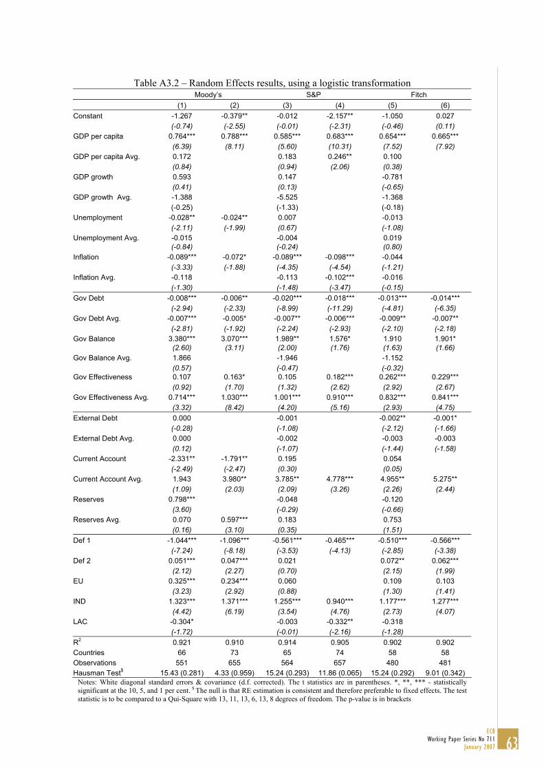
Table A3.2 – Random Effects results, using a logistic transformation

Moody’s S&P Fitch (1) (2) (3) (4) (5) (6)

Constant -1.267 -0.379** -0.012 -2.157** -1.050 0.027 (-0.74) (-2.55) (-0.01) (-2.31) (-0.46) (0.11) GDP per capita 0.764*** 0.788*** 0.585*** 0.683*** 0.654*** 0.665*** (6.39) (8.11) (5.60) (10.31) (7.52) (7.92) GDP per capita Avg. 0.172 0.183 0.246** 0.100 (0.84) (0.94) (2.06) (0.38) GDP growth 0.593 0.147 -0.781 (0.41) (0.13) (-0.65) GDP growth Avg. -1.388 -5.525 -1.368 (-0.25) (-1.33) (-0.18) Unemployment -0.028** -0.024** 0.007 -0.013 (-2.11) (-1.99) (0.67) (-1.08) Unemployment Avg. -0.015 -0.004 0.019 (-0.84) (-0.24) (0.80) Inflation -0.089*** -0.072* -0.089*** -0.098*** -0.044 (-3.33) (-1.88) (-4.35) (-4.54) (-1.21) Inflation Avg. -0.118 -0.113 -0.102*** -0.016 (-1.30) (-1.48) (-3.47) (-0.15) Gov Debt -0.008*** -0.006** -0.020*** -0.018*** -0.013*** -0.014*** (-2.94) (-2.33) (-8.99) (-11.29) (-4.81) (-6.35) Gov Debt Avg. -0.007*** -0.005* -0.007** -0.006*** -0.009** -0.007** (-2.81) (-1.92) (-2.24) (-2.93) (-2.10) (-2.18) Gov Balance 3.380*** 3.070*** 1.989** 1.576* 1.910 1.901* (2.60) (3.11) (2.00) (1.76) (1.63) (1.66) Gov Balance Avg. 1.866 -1.946 -1.152 (0.57) (-0.47) (-0.32) Gov Effectiveness 0.107 0.163* 0.105 0.182*** 0.262*** 0.229*** (0.92) (1.70) (1.32) (2.62) (2.92) (2.67) Gov Effectiveness Avg. 0.714*** 1.030*** 1.001*** 0.910*** 0.832*** 0.841*** (3.32) (8.42) (4.20) (5.16) (2.93) (4.75) External Debt 0.000 -0.001 -0.002** -0.001* (-0.28) (-1.08) (-2.12) (-1.66) External Debt Avg. 0.000 -0.002 -0.003 -0.003 (0.12) (-1.07) (-1.44) (-1.58) Current Account -2.331** -1.791** 0.195 0.054 (-2.49) (-2.47) (0.30) (0.05) Current Account Avg. 1.943 3.980** 3.785** 4.778*** 4.955** 5.275** (1.09) (2.03) (2.09) (3.26) (2.26) (2.44) Reserves 0.798*** -0.048 -0.120 (3.60) (-0.29) (-0.66) Reserves Avg. 0.070 0.597*** 0.183 0.753 (0.16) (3.10) (0.35) (1.51) Def 1 -1.044*** -1.096*** -0.561*** -0.465*** -0.510*** -0.566*** (-7.24) (-8.18) (-3.53) (-4.13) (-2.85) (-3.38) Def 2 0.051*** 0.047*** 0.021 0.072** 0.062*** (2.12) (2.27) (0.70) (2.15) (1.99) EU 0.325*** 0.234*** 0.060 0.109 0.103 (3.23) (2.92) (0.88) (1.30) (1.41) IND 1.323*** 1.371*** 1.255*** 0.940*** 1.177*** 1.277*** (4.42) (6.19) (3.54) (4.76) (2.73) (4.07) LAC -0.304* -0.003 -0.332** -0.318

(-1.72) (-0.01) (-2.16) (-1.28) R2 0.921 0.910 0.914 0.905 0.902 0.902 Countries 66 73 65 74 58 58 Observations 551 655 564 657 480 481 Hausman Test$ 15.43 (0.281) 4.33 (0.959) 15.24 (0.293) 11.86 (0.065) 15.24 (0.292) 9.01 (0.342)

Notes: White diagonal standard errors & covariance (d.f. corrected). The t statistics are in parentheses. *, **, *** - statistically significant at the 10, 5, and 1 per cent. $ The null is that RE estimation is consistent and therefore preferable to fixed effects. The test statistic is to be compared to a Qui-Square with 13, 11, 13, 6, 13, 8 degrees of freedom. The p-value is in brackets

63ECB



European Central Bank Working Paper Series

For a complete list of Working Papers published by the ECB, please visit the ECB’s website(http://www.ecb.int)

680 “Comparing alternative predictors based on large-panel factor models” by A. D’Agostino and D. Giannone, October 2006.

681 “Regional inflation dynamics within and across euro area countries and a comparison with the US” by G. W. Beck, K. Hubrich and M. Marcellino, October 2006.

682 “Is reversion to PPP in euro exchange rates non-linear?” by B. Schnatz, October 2006.

683 “Financial integration of new EU Member States” by L. Cappiello, B. Gérard, A. Kadareja and S. Manganelli, October 2006.

684 “Inflation dynamics and regime shifts” by J. Lendvai, October 2006.

685 “Home bias in global bond and equity markets: the role of real exchange rate volatility” by M. Fidora, M. Fratzscher and C. Thimann, October 2006

686 “Stale information, shocks and volatility” by R. Gropp and A. Kadareja, October 2006.

687 “Credit growth in Central and Eastern Europe: new (over)shooting stars?” by B. Égert, P. Backé and T. Zumer, October 2006.

688 “Determinants of workers’ remittances: evidence from the European Neighbouring Region” by I. Schiopu and N. Siegfried, October 2006.

689 “The effect of financial development on the investment-cash flow relationship: cross-country evidence from Europe” by B. Becker and J. Sivadasan, October 2006.

690 “Optimal simple monetary policy rules and non-atomistic wage setters in a New-Keynesian framework” by S. Gnocchi, October 2006.

691 “The yield curve as a predictor and emerging economies” by A. Mehl, November 2006.

692 “Bayesian inference in cointegrated VAR models: with applications to the demand for euro area M3” by A. Warne, November 2006.

693 “Evaluating China’s integration in world trade with a gravity model based benchmark” by M. Bussière and B. Schnatz, November 2006.

694 “Optimal currency shares in international reserves: the impact of the euro and the prospects for the dollar” by E. Papaioannou, R. Portes and G. Siourounis, November 2006.

695 “Geography or skills: What explains Fed watchers’ forecast accuracy of US monetary policy?” by H. Berger, M. Ehrmann and M. Fratzscher, November 2006.

696 “What is global excess liquidity, and does it matter?” by R. Rüffer and L. Stracca, November 2006.

697 “How wages change: micro evidence from the International Wage Flexibility Project” by W. T. Dickens, L. Götte, E. L. Groshen, S. Holden, J. Messina, M. E. Schweitzer, J. Turunen, and M. E. Ward, November 2006.

698 “Optimal monetary policy rules with labor market frictions” by E. Faia, November 2006.

65ECB


699 “The behaviour of producer prices: some evidence from the French PPI micro data” by E. Gautier, December 2006.

700 “Forecasting using a large number of predictors: Is Bayesian regression a valid alternative toprincipal components?” by C. De Mol, D. Giannone and L. Reichlin, December 2006.

701 “Is there a single frontier in a single European banking market?” by J. W. B. Bos and H. Schmiedel, December 2006.

702 “Comparing financial systems: a structural analysis” by S. Champonnois, December 2006.

703 “Comovements in volatility in the euro money market” by N. Cassola and C. Morana, December 2006.

704 “Are money and consumption additively separable in the euro area? A non-parametric approach” by B. E. Jones and L. Stracca, December 2006.

705 “What does a technology shock do? A VAR analysis with model-based sign restrictions” by L. Dedola and S. Neri, December 2006.

706 “What drives investors’ behaviour in different FX market segments? A VAR-based returndecomposition analysis” by O. Castrén, C. Osbat and M. Sydow, December 2006.

707 “Ramsey monetary policy with labour market frictions” by E. Faia, January 2007.

708 “Regional housing market spillovers in the US: lessons from regional divergences in a common monetary policy setting” by I. Vansteenkiste, January 2007.

709 “Quantifying and sustaining welfare gains from monetary commitment” by P. Levine, P. McAdam and J. Pearlman, January 2007.

710 “Pricing of settlement link services and mergers of central securities depositories” by J. Tapking, January 2007.

711 “What “hides” behind sovereign debt ratings?” by A. Afonso, P. Gomes and P. Rother, January 2007.

ISSN 1561081-0

9 7 7 1 5 6 1 0 8 1 0 0 5

working paper series - european central bank · sovereign debt ratings? 1 by antónio afonso 2,...

Documents