wildlife and landscape ecology || applications of fractal geometry in wildlife biology

2 Applications of Fractal Geometry in Wildlife Biology

BRUCE T. MILNE

2.1 Introduction

Unlike simple physical systems, such as frictionless pendula and leaking buckets, ecosystems possess complexities that have limited biologists' ability to describe, predict, and manage natural resources. Complexity can be addressed with tools to assess spatial pattern over vast expanses (e.g., geographic information systems and remote sensing), to uncover persistent interactions over space and time (Cressie 1991, Deutsch and JourneI1992), and to discover simplicity in the face of chaotic changes (Tilman and Wedin 1991, Sole et al. 1992, Kauffman 1993, Plotnick and McKinney 1993, Peak, Chapter 3). Techniques to unravel spatial and temporal complexity involve purposeful manipulation of the scale of observation to discover how phenomena change steadily, and predictably, with scale.

Ecology and wildlife biology share an awareness that natural complexity varies predictably with scale, in both space and time (Urban et al. 1987, Senft et al. 1987, Delcourt and Delcourt 1988). For example, hierarchical complexity can be discerned by measuring nature at a variety of scales (Allen and Starr 1982). By observing mortality due to old age and mortality due to predation, the observer jumps from the population level of organization to the community level (Allen and Hoekstra 1992). Reviews about scale (Wiens 1989, Levin 1992, Schneider 1994) and synthetic evaluations of complexity (Holling 1992) suggest that observations made at multiple scales are key to unraveling natural complexity.

Bruce T. Milne is Associate Professor of Biology in the Department of Biology, University of New Mexico. He is also principal investigator of the Sevilleta Long Term Ecological Research project. His research focuses on the role of spatial complexity in landscapes. Since 1985 he has explored the use of fractal geometry for the characterization of landscape patterns and has applied percolation theory in studies of beetle diffusion and ecotone structure. Recent interest in the biological controls of ecotones has led to investigations of soil, water, and energy balance models.

32

J. A. Bissonette (ed.), Wildlife and Landscape Ecology© Springer-Verlag New York Inc. 1997

2. Applications of Fractal Geometry in Wildlife Biology 33

The word scale has many meanings, but in general it refers to the resolution at which patterns are measured, perceived, or represented. It is helpful to break the notion of scale into several components, namely, grain, extent, lag, and window length (Milne 1991a). These four components can be manipulated to reveal different properties of a study area or a species distribution. Grain is the smallest resolvable unit of study, for example a 1 x 1 m quadrat. On a digital map, a grain is one "cell" or "pixel," which represents the vegetation type present, the number of animals present, or some abiotic condition of the landscape. Grain generally determines the lower limit of what can be studied. Extent is the width of a study area, the boundary of a map, a species range, or the duration of a study. Extent determines the limit to how many grains can be observed and the limit of the largest patterns that can be observed (see Magnuson 1990).

Analyses of complexity involve comparisons of grains separated by a given distance. For example, we could easily compare all the grains that are 60m apart; the distance 60 is called a lag distance. The results of comparisons vary predictably with lag (Burrough 1986, Cressie 1991, Rossi et al. 1992), and the dependence provides a very useful characterization of spatial complexity. For example, one could walk along recording elevation every 60 paces. A graph of the elevation at one location versus that at the next would portray the correlation between elevations measured at a lag of 60 paces. Estimating the correlations at 5, 10, 30, and 120 pace lags would reveal how the correlation changes with scale, thereby providing a characterization of terrain roughness.

Rather than considering one point at a time, a window (e.g., a quadrat or plot) surrounds a set of grains from which a statistical property, such as a mean, is measured. As for lags, statistical properties can be studied as a function of window size to reveal regularities in complex patterns.

Regardless of how scale is treated technically, many characteristics of landscapes that pertain to wildlife and habitat management vary with scale, such as vegetation (Palmer 1988), animal density (Peters 1983), patch geometry (Krummel et al. 1987) or resource availability (Milne 1992a). Changes in pattern with scale reflect transitions between the controlling influence of one environmental factor over another (Johnson et al. 1992). There are two ways in which factors operate across a range of scales, i.e., grain sizes, lags, or window sizes. First, a constraint such as a streambed may interact with something else, such as stream discharge, in a consistent way across a range of scales, as from 1st- to 10th-order streams. Second, the controlling factors may change abruptly, as when interspecific competition outweighs intraspecific competition (Yamamura 1976) to create a discontinuity in a pattern on the landscape, such as at an ecotone boundary (Milne et al. 1996). It is important for management purposes to: (1) identify what the major controlling factors are (e.g., forage availability versus climate) and (2) to quantify the "domain" of scales (Wiens 1989) over which a manageable factor operates, e.g., transmission distances of a disease. Tools

34 B.T. Milne

described below detect such domains and characterize the scales over which a single factor operates (see Milne 1992b).

The main purpose of this chapter is to illustrate the fundamental notions of fractal geometry (Mandelbrot 1982) as they apply to wildlife biology. By definition, fractal geometry requires a multiscale approach to studies of nature. It is useful to ignore the puzzling details of fractal geometry, which are available in many reviews (e.g., Feder 1988, Peitgen and Saupe 1988, Milne 1991a) until an intuitive understanding is had of the issues, problems, and insights to be gained by the use of fractal geometry. Indeed, the beauty and usefulness of fractal geometry are closely tied to the intuition about natural complexity that is captured by rather simple quantitative approaches. Specific applications to wildlife biology included here are:

1. an estimate of bald-eagle nest density along a coastline 2. estimation of red-cockaded woodpecker habitat area for the southern

United States 3. models of the fluxes of water, nitrogen, and reproductive energy costs for

herbivorous mammals living on fractal landscapes 4. modification of the classic species-area relation to accommodate the

fractal geometry of islands 5. aggregation of fine-scale maps to coarse resolution as in GAP analysis 6. analyses of pelican population changes in relation to climate fluctuations 7. visualization of habitat edges at multiple scales.

2.1.1 Allometry: Biological Scale Dependence Species effectively operate at different scales by virtue of physiological and morphometric characteristics that vary predictably with body mass. Allometry describes how physical, morphological, physiological, and behavioral traits vary with body size both in animals (Peters 1983) and plants (Niklas 1994). Allometry affects reproductive success via clutch size, foraging rates, and traits related to locomotion, thermal regulation, and demography. In general, mammals respire, grow, and reproduce as the 3/4 power of body mass while physiological rates per unit mass vary as the -+power of mass (Peters 1983). Allometrically controlled defecation rates and nutritional requirements pertain directly to ecosystem function because small animals process energy and wastes at vastly different rates than do large animals. Allometry in animals is tied closely to energetic requirements that have been adjusted evolutionarily to trade off the benefits of gathering energy against the rate at which energy can be converted to offspring (Brown et al. 1993). Tradeoffs between small size, which confers an advantage during reproduction, and large size, with associated low costs of trans-


port to find food, indicate that the optimal mammalian body size is 100 g (Brown et al. 1993). For purposes of this chapter, I consider animals >100g and thereby assume that relevant traits increase or decrease steadily with body mass.

Over broad areas, species interact with continental margins, mountain ranges, landscapes, and patches (Senft et al. 1987) in very different ways depending upon strong interactions between allometry, habitat requirements, and the geographic distribution of habitat. For instance, foragers select individual plants depending on palatability or caloric supply and simultaneously select among patches of plants, landscapes, and regions depending on food availability (Senft et al. 1987), safety from predation, competitive regimes, mate availability, and climatic factors (Root 1988). Source-sink (Pulliam and Danielson 1991), neighborhood (Clements 1905), and proximity effects (Milne et al. 1989) contribute to a species distribution in somewhat indirect ways. Thus, the myriad ultimate factors that regulate a species distribution interact, some locally and others over broad areas.

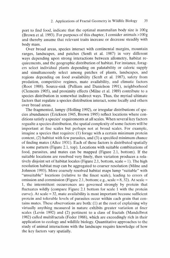
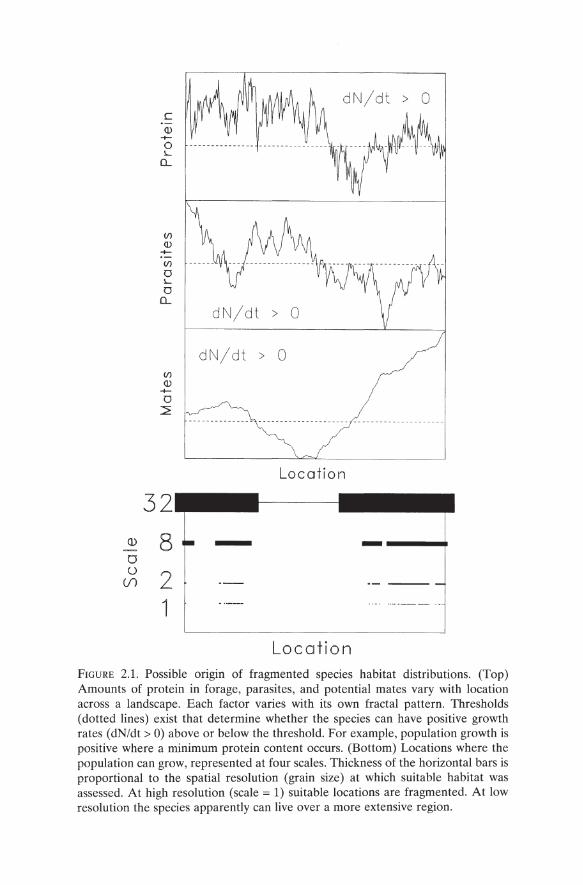
The fragmented, lumpy (Holling 1992), or irregular distributions of species abundances (Erickson 1945, Brown 1995) reflect locations where conditions satisfy a species' requirements at all scales. When several key factors regualte a species distribution, the spatial complexity of some factors will be important at fine scales but perhaps not at broad scales. For example, imagine a species that requires: (1) forage with a certain minimum protein content, (2) habitat with few parasites, and (3) a specified minimum chance of finding mates (Allee 1931). Each of these factors is distributed spatially in some pattern (Figure 2.1, top). Locations with suitable combinations of food, parasites, and mates can be mapped (Figure 2.1, bottom). If the suitable locations are resolved very finely, then variation produces a relatively disjoint set of habitat locales (Figure 2.1, bottom, scale = 1). The high resolution habitat map can be aggregated to coarser resolution (Milne and Johnson 1993). More coarsely resolved habitat maps lump "suitable" with "unsuitable" locations (relative to the finest scale), leading to errors of omission and commission (Figure 2.1, bottom; e.g., scale = 8, 32). At scale =

1, the intermittent occurrences are governed strongly by protein that fluctuates wildly (compare Figure 2.1 bottom for scale 1 with the protein curve). At scale = 32, mate availability is most important because sufficient protein and tolerable levels of parasites occur within each grain that contains mates. These observations are both: (1) at the root of explaining why virtually anything measured in nature exhibits greater variation at finer scales (Levin 1992) and (2) pertinent to a class of fractals (Mandelbrot 1982) called multifractals (Feder 1988), which are exceedingly rich in their application to ecology and wildlife biology. Quantitative approaches to the study of animal interactions with the landscape require knowledge of how the key factors vary spatially.

(I)

o ()

(f)

c Q) --o L

0.-

32

8

2 1

dN/dt >

Location

----....

Location FIGURE 2.1. Possible origin of fragmented species habitat distributions. (Top) Amounts of protein in forage, parasites, and potential mates vary with location across a landscape. Each factor varies with its own fractal pattern. Thresholds (dotted lines) exist that determine whether the species can have positive growth rates (dN/dt > 0) above or below the threshold. For example, population growth is positive where a minimum protein content occurs. (Bottom) Locations where the population can grow, represented at four scales. Thickness of the horizontal bars is proportional to the spatial resolution (grain size) at which suitable habitat was assessed. At high resolution (scale = 1) suitable locations are fragmented. At low resolution the species apparently can live over a more extensive region.


2.2 The Notion of Scale Dependence

As a graduate student in 1982, I studied species diversity on the coast of Maine, USA (Milne and Forman 1986). The study was designed to test Simpson's (1964) peninsula diversity hypothesis that the number of species decreases with distance from the mainland. In search of independent replicate peninsulas, I spent many frustrating days trying to overcome what I eventually learned was the hallmark of a fractal: every small peninsula was but a knob on the side of a yet larger one (see the map in Figure 2.1 in Milne and Forman 1986, or virtually any map of a jagged coastline). Thus, no peninsula was "independent" of others, and the assumption of independent replicates (Hurlbert 1984) could not be satisfied. I learned that a profound stumbling block to an otherwise pedestrian study is a fertile topic in itself.

Indeed, coastlines remain the archetypal fractal because they illustrate the concepts of self-similarity and scale dependence. Self-similar patterns can be magnified to reveal more of the same pattern at increasingly finer scales. The classic example of scale dependence is Richardson's (1960) analysis of the coast of Britain. By asking "How long is the coast of Britain?" we discover that the length depends upon the resolution at which it is measured (Mandelbrot 1982), i.e., is scale dependent. At first this seems paradoxical, as we expect that a single length must exist. However, a simple exercise illustrates notions of both scale dependence and selfsimilarity.

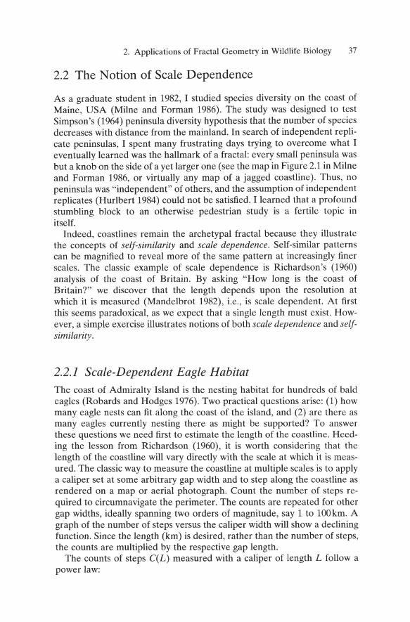
2.2.1 Scale-Dependent Eagle Habitat The coast of Admiralty Island is the nesting habitat for hundreds of bald eagles (Robards and Hodges 1976). Two practical questions arise: (1) how many eagle nests can fit along the coast of the island, and (2) are there as many eagles currently nesting there as might be supported? To answer these questions we need first to estimate the length of the coastline. Heeding the lesson from Richardson (1960), it is worth considering that the length of the coastline will vary directly with the scale at which it is measured. The classic way to measure the coastline at multiple scales is to apply a caliper set at some arbitrary gap width and to step along the coastline as rendered on a map or aerial photograph. Count the number of steps required to circumnavigate the perimeter. The counts are repeated for other gap widths, ideally spanning two orders of magnitude, say 1 to 100km. A graph of the number of steps versus the caliper width will show a declining function. Since the length (km) is desired, rather than the number of steps, the counts are multiplied by the respective gap length.

The counts of steps C(L) measured with a caliper of length L follow a power law:

38 B.T. Milne

(1)

where Dc is a fractal dimension estimated by the caliper method, and b is a constant; the symbol C(L) is subscript notation, not multiplication.

In geometry, a dimension specifies how to relate a small part of something to the whole. For example, there are 8 cells along one edge of a checkerboard and 82 = 64 cells in all. The 8 is squared because the board is a two-dimensional plane. Similarly, the number of inches in a foot is 12 = 121; the implicit exponent 1 indicates that a foot is a linear measure. The dimension 3 is used to relate the edge of a cube to its volume. Fractal objects, such as coastlines, generally have noninteger dimensions such as 1.28, indicating that the bends in the coastline tend to fill the plane in which it is embedded; the coastline does not occupy the entire two-dimensional plane (Figure 2.2). Rough terrain can be described as a bent and folded sheet that tends to fill the three-dimensional space surrounding the surface (Figure 2.3). Thus, terrain exhibits dimensions between 2 and 3 (Turcotte 1992). Fractal dimensions relate to the jaggedness of curves or the roughness of surfaces.

At first, the smallness of dimensions and, worse yet, the small difference between a dimension of, say, 1.2 and 1.3, may lead one to wonder how they could have much effect on wildlife. However, the dimensions are exponents in scaling relations like eq. 1, and thus a small change in the exponent can have a big impact on that which is measured, e.g., the coastline length.

Nests 800.-----------------------,

,-.... . E

..c 600 -t--

Ol C Q)

Q)

c400 +(J)

o o

(.)

•

Admiralty Island

.:e(L) = 715.7 L1- Dc

o = 1.25 c

2000~---1~O----~20----~3~O----4~O~~50

Caliper width (km)

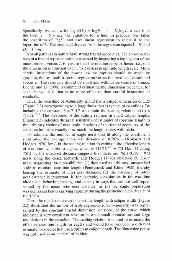
FIGURE 2.2. Distribution of bald-eagle nests (after Robards and Hodges 1976) and fractal geometry of Admiralty Island. The caliper dimension Dc is related to the caliper width L used to estimate coastline length 2'(L).


o • :::::0.5 •• • •

1

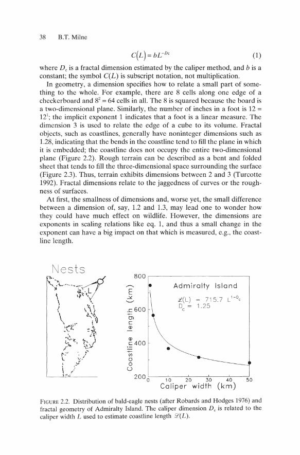
2 D :::::2.3 r:;;7 FIGURE 2.3. Euclidean and fractal dimensions of representative patterns. Euclidean sets such as points, lines, and planes have integer dimensions 0, 1, and 2, respectively. Fractals include sets of points along a line, a curve with fluctuations at all scales CD '" 1.28), or rough terrain that resembles a bent and folded sheet with D '" 2.3.

Patterns with noninteger dimensions are called fractals. Written as a power of L, measurements of fractals (e.g., eq. 1) reflect the idea that there is no single scale that best describes a fractal. Rather, an explicit reference to the scale is needed to infer the length, amount, density, or roughness of a fractal. Here is the most important point when using fractal geometry to solve problems in wildlife biology: the animal is the caliper. For example, on average, the area of an animal's home range (i.e., its caliper) increases with body mass because larger animals need more food and have to cover more ground to find it. Thus, a O.lkg animal needs much less area than a 100kg animal. If we consider the populations of these two species we can imagine that: (1) small animals reach higher densities on a given fractal landscape (Morse et al. 1985), and (2) if the species happen to occupy coastlines, the small species will perceive a longer coastline than the large species. Moreover, let us assume that the two species use the same resource, such as grass. Then places where the resource is relatively dense for the small species will be different from those where the grass is dense for large species (Milne 1992a, Milne et al. 1992). The scale dependence of suitable habitat has profound implications for the coexistence of species.

Returning to the eagle example, counts of steps of length L are converted to actual length of coastline 2'( L) by multiplying counts by the length of the step:

(2)

By logarithmic transformation, eq. 2 can be written as the equation of a line, and linear regression can be used to estimate the slope, which is 1 - DC"

40 B.T. Milne

Specifically, we can write log .'?(L) = 10gb + 1 - DJogL which is in the form y = b + mx, the equation for a line. In practice, one takes the logarithm of .'?(L) and uses linear regression to relate it to the logarithm of L. The predicted slope m from the regression equals 1- Dc and Dc = 1- m.

Not all patterns in nature have strong fractal properties. The appropriateness of a fractal representation is assessed by inspecting a log-log plot of the measurement versus L to ensure that the relation appears linear, i.e., that the dimension is constant over 1 to 2 orders magnitude length scale. More careful inspections of the power law assumption should be made by graphing the residuals from the regression versus the predicted values and versus L. The residuals should be small and without curvature or trends. Loehle and Li (1996) recommend estimating the dimension piecemeal for each change in L that is no more effective than careful inspection of residuals.

Thus, the coastline of Admiralty Island has a caliper dimension of 1.25 (Figure 2.2) corresponding to a jaggedness that is typical of coastlines. By including the constant b = 715.7 we obtain the scaling relation .'l'(L) = 715.7 C 025 • The steepness of the scaling relation at small caliper lengths (Figure 2.2) indicates the great sensitivity of estimates of coastline length to the arbitrary choice of map scale. Analysis of the fractal geometry of the coastline indicates exactly how much the length varies with scale.

To estimate the number of eagle nests that fit along the coastline, I substituted the average inter-nest distance of 0.782km (Robards and Hodges 1976) for L in the scaling relation to estimate the effective length of coastline available to eagles, which is 715.7 C 025 = 761.1 km. Dividing 761.1 by the internest distance suggests that there are 761.110.782 = 973 nests along the coast. Robards and Hodges (1976) observed 80 fewer nests, suggesting three possibilities: (1) they used an arbitrary, unspecified scale to estimate coastline length (Pennycuick and Kline 1986), thereby biasing the estimate of inter-nest distance; (2) the variance of internest distance is important, if, for example, convolutions in the coastline alter social behavior, spacing, and density in ways that are not well represented by the mean inter-nest distance; or (3) the eagle population was depressed below carrying capacity during the pesticide-laden decade of the 1970s.

Thus, the regular decrease in coastline length with caliper width (Figure 2.2) illustrated the notion of scale dependence. Self-similarity was represented by the constant fractal dimension, or slope, of the curve, which indicated a very consistent relation between small crenulations and large undulations in the coastline. The scaling relation was used to estimate the effective coastline length for eagles and would have produced a different estimate for species that use a different caliper length. The dimension per se was not used as an "index" of habitat.


2.2.2 Box Dimension and the Red-Cockaded Woodpecker Coastlines are quasi I-dimensional structures that require the caliper method to estimate the dimension. In contrast, habitats that are better described as patches require different methods to measure scale dependence and self-similarity. As for Admiralty Island, one application is to estimate how much habitat is available to species that encounter the landscape at scales other than those used by cartographers. The box dimension (Mandelbrot 1982, Voss 1988, Milne 1991a) provides a scaling relation appropriate for binary maps of patches. Expectations for the box dimension are that it will equal 0 when a habitat map is composed of a single point (Figure 2.3) and will range up to a value of 2 when the habitat occurs everywhere at all scales. The pattern analysis literature generally poses a trichotomy of pattern types, namely random, regular, and clumped (Pielou 1977). Interestingly, both random and regular patterns share a box dimension equal to 2 (for boxes greater than the average inter-patch distance in regular patterns, such as checkerboards). In both cases the number of grains increases strictly as the square of the window length. By this criterion both patterns are best thought of as homogeneous or lacking in contagion.

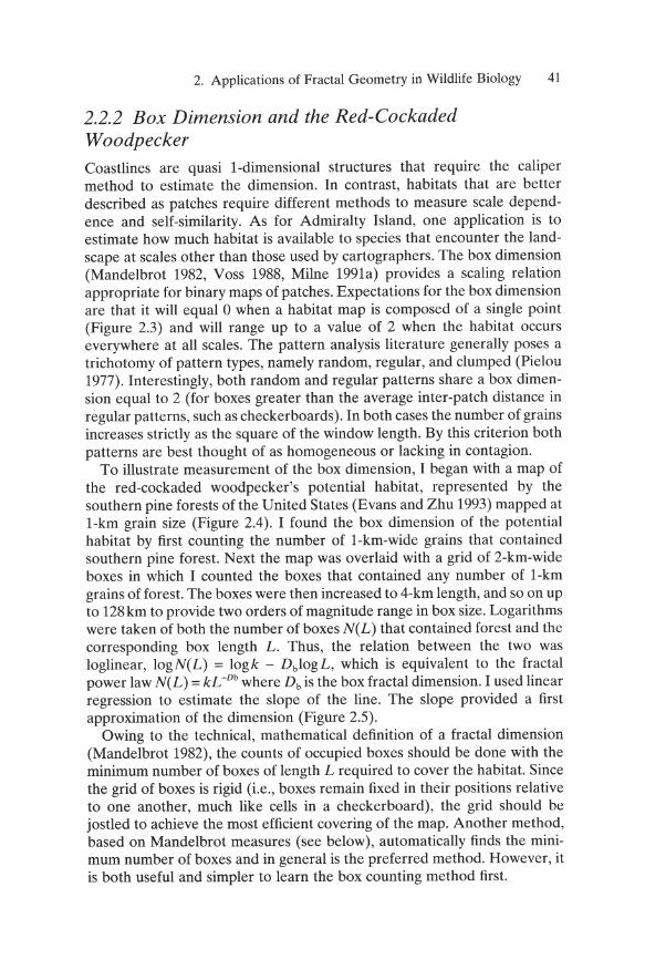
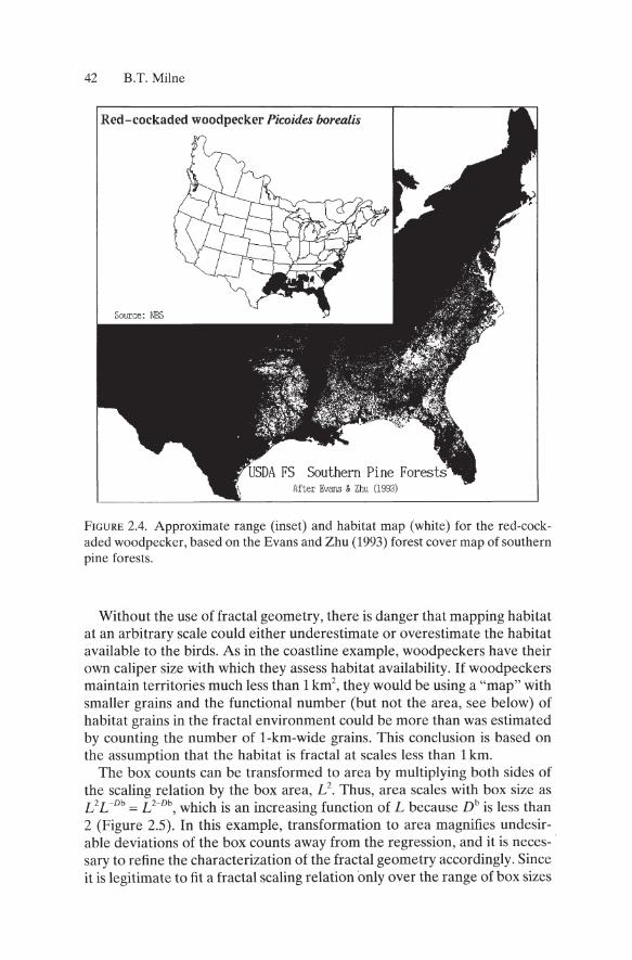
To illustrate measurement of the box dimension, I began with a map of the red-cockaded woodpecker's potential habitat, represented by the southern pine forests of the United States (Evans and Zhu 1993) mapped at l-km grain size (Figure 2.4). I found the box dimension of the potential habitat by first counting the number of l-km-wide grains that contained southern pine forest. Next the map was overlaid with a grid of 2-km-wide boxes in which I counted the boxes that contained any number of l-km grains of forest. The boxes were then increased to 4-km length, and so on up to 128 km to provide two orders of magnitude range in box size. Logarithms were taken of both the number of boxes N( L) that contained forest and the corresponding box length L. Thus, the relation between the two was loglinear, 10gN(L) = logk - DblogL, which is equivalent to the fractal power law N( L) = kL -Db where Db is the box fractal dimension. I used linear regression to estimate the slope of the line. The slope provided a first approximation of the dimension (Figure 2.5).

Owing to the technical, mathematical definition of a fractal dimension (Mandelbrot 1982), the counts of occupied boxes should be done with the minimum number of boxes of length L required to cover the habitat. Since the grid of boxes is rigid (i.e., boxes remain fixed in their positions relative to one another, much like cells in a checkerboard), the grid should be jostled to achieve the most efficient covering of the map. Another method, based on Mandelbrot measures (see below), automatically finds the minimum number of boxes and in general is the preferred method. However, it is both useful and simpler to learn the box counting method first.

42 B.T. Milne

Red-cockaded woodpecker Picoides borealis

After Evans & Zhu (1993)

FIGURE 2.4. Approximate range (inset) and habitat map (white) for the red-cockaded woodpecker, based on the Evans and Zhu (1993) forest cover map of southern pine forests.

Without the use of fractal geometry, there is danger that mapping habitat at an arbitrary scale could either underestimate or overestimate the habitat available to the birds. As in the coastline example, woodpeckers have their own caliper size with which they assess habitat availability. If woodpeckers maintain territories much less than 1 km2, they would be using a "map" with smaller grains and the functional number (but not the area, see below) of habitat grains in the fractal environment could be more than was estimated by counting the number of I-km-wide grains. This conclusion is based on the assumption that the habitat is fractal at scales less than 1 km.

The box counts can be transformed to area by multiplying both sides of the scaling relation by the box area, L2. Thus, area scales with box size as L 2L-Db = L 2- Db, which is an increasing function of L because Db is less than 2 (Figure 2.5). In this example, transformation to area magnifies undesirable deviations of the box counts away from the regression, and it is necessary to refine the characterization of the fractal geometry accordingly. Since it is legitimate to fit a fractal scaling relation only over the range of box sizes


for which the estimates of area fit a power law, I fit the curve for area using length >lOkm. Thus, the area dimension Da = 1.76 (Figure 2.5).

Above lOkm (Figure 2.5), factors related to the geometry of terrain probably produce a reasonable fractal pattern by limiting the distribution of forests via gradients in soil moisture and solar radiation (Frank and Inouye 1994). At scales below 10km considerably less habitat is available than would be expected from the fractal relation, possibly because of land use practices (Krummel et a1. 1987) or seed dispersal limitation, which aggregate pine forests at short scales. Aggregation, or contagion, reduces the small fragments of forest that would be expected to persist if a fractal generating process were operating. Based on the argument that fractal habitat pattern enables species of different sizes to occupy different places within a landscape (Milne 1992a), the lack of fractal structure below 10km implies that species of disparate body size may be forced to occupy the same, relatively large patches. Before reaching equilibrium, there could be an increase in species richness within a patch and also increased competition. Evidence of elevated richness due to contagion would come from

• 10 5 (f) Q)

x o

....0

'0 10 4

•

0

0

1 Box

/ / /0 Do

Db= 1.66

10 length (km)

1.76 1 0 6 0

~

N

E .:::::. "---'"'

0 Q) ~

«

• 1 0 5 100

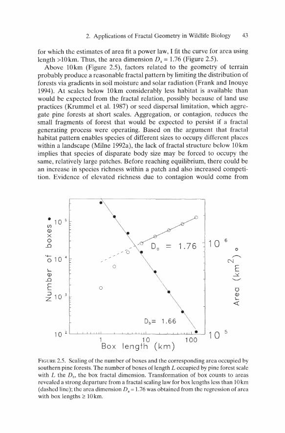
FIGURE 2.S. Scaling of the number of boxes and the corresponding area occupied by southern pine forests. The number of boxes of length L occupied by pine forest scale with L the Db, the box fractal dimension. Transformation of box counts to areas revealed a strong departure from a fractal scaling law for box lengths less than 10 km (dashed line); the area dimension Da = 1.76 was obtained from the regression of area with box lengths 2': 10 km.

44 B.T. Milne

studies of bird species richness in forest islands expressed per unit of patch area. Expressed per unit area, both richness and competition should be highest in landscapes with relatively few small patches, i.e., with area-scale relations that violate fractal scaling laws at fine scales. Support for the competition effect would argue for the deliberate creation or preservation of landscapes with a wide variety of patch sizes (Milne 1991b, Forman 1995). A very real trade-off in this design strategy relates to the greater success of nest parasites in small patches. However, costs due to parasitism might be outweighed by the benefits of the very large patches that are necessary to produce a fractal pattern that spans several orders of magnitude.

2.3 Mandelbrot Measures: Relations to the Landscape

The fractal properties of Admiralty Island and woodpecker habitat illustrate the statistical regularity and predictive power of fractal geometry. Equally useful insights come from mapping resources, habitats, or organisms at different scales. Such maps enable the statistical properties of fractals to be related directly to the ground (Milne 1992a), with potential applications in resource thinning and planting operations (Milne 1993). The statistical relations also enable assessments of the encounter rate between predators and prey (Mangel and Adler 1994). Geometrical treatments are useful for predicting species interactions through competition or predation, which may be altered considerably by landscape pattern (Spalinger and Hobbs 1992, Keitt and Johnson 1995).

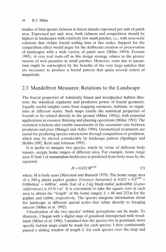
It is useful to imagine two species, which by virtue of different body masses, occupy home ranges of different sizes. For example, home range area H (km2) of mammalian herbivores is predicted from body mass by the equation:

H = 0.032Af!998 (3)

where M is body mass (Harestad and Bunnell 1979). The home range area of a 200-g plains pocket gopher (Geamys bursarius) is 0.032 x 0.20998 = 0.0064km2 = 6400m2, while that of a 2-kg black-tailed jackrabbit (Lepus califamicus) is 63,911 m2. It is convenient to take the square root of each area to obtain the "length" of the home ranges; L = 80 and 252m for the gopher and rabbit, respectively. The species integrate information about the landscape at different spatial scales that relate directly to foraging success (Milne et al. 1992).

Visualization of the two species' habitat perceptions can be made. To illustrate, I began with a digital map of grassland interspersed with woodlands (Milne et al. 1996). I assumed that the species live in grassland; more specific habitat maps could be made for each species. I then continuously passed a sliding window of length L for each species over the map and


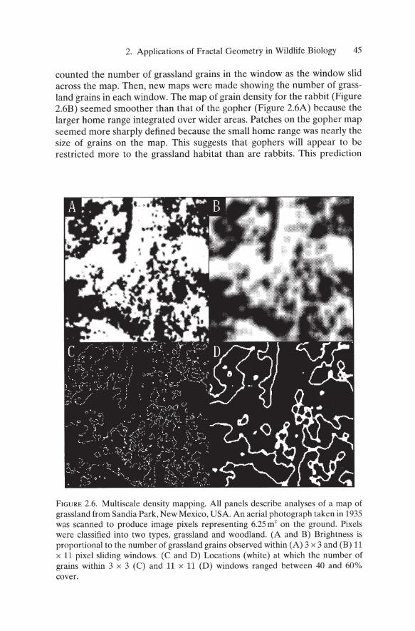
counted the number of grassland grains in the window as the window slid across the map. Then, new maps were made showing the number of grassland grains in each window. The map of grain density for the rabbit (Figure 2.6B) seemed smoother than that of the gopher (Figure 2.6A) because the larger home range integrated over wider areas. Patches on the gopher map seemed more sharply defined because the small home range was nearly the size of grains on the map. This suggests that gophers will appear to be restricted more to the grassland habitat than are rabbits. This prediction

FIGURE 2.6. Multiscale density mapping. All panels describe analyses of a map of grassland from Sandia Park, New Mexico, USA. An aerial photograph taken in 1935 was scanned to produce image pixels representing 6.25 m2 on the ground. Pixels were classified into two types, grassland and woodland. (A and B) Brightness is proportional to the number of grassland grains observed within (A) 3 x 3 and (B) 11 x 11 pixel sliding windows. (C and D) Locations (white) at which the number of grains within 3 x 3 (C) and 11 x 11 (D) windows ranged between 40 and 60% cover.

46 B. T. Milne

would be falsified if: (1) population densities were well below carrying capacity, and (2) if the nongrassland areas function as barriers, thereby reducing access to grassland within a window.

I incorporated the idea that some species prefer "edge" habitat by mapping only windows that contained 40 to 60% grassland cover (Figure 2.6C, D). The "edges" for rabbits were considerably smoother and at different locations than those for gophers. Here, I simply varied the window size and held the edge definition constant to reveal that changes in scale alter the amount of edge and locations of the edges (Milne 1992a), much as changes in caliper width alter estimates of coastline length.

As a technical aside, the counts of grassland cells, mapped at each location, form a geometric measure (Morgan 1988). When the measures are restricted to windows whose centers are occupied by the cover type of interest, in this case grassland, the measures are called Mandelbrot measures (Voss 1988). Since map boundaries prevent the centers of big windows from visiting the same set of locations as the centers of small windows, only locations common to both large and small windows were mapped (Figure 2.6).

2.3.1 Scaling of Mandelbrot Measures One of the most useful aspects of fractal analyses based on Mandelbrot measures is a well-developed, and still developing, methodology to quantify the statistical behavior of subsets of fractal patterns. The methodology has been reviewed many times (Feder 1988, Voss 1988, Milne 1991a, 1992a, Sole and Manrubia 1995) and applied in fairly advanced ways for studies of the correlation between two or more fractal sets. e.g., as for studies of two or more species (Scheuring and Riedi 1994) and for a fractal thinning procedure designed to preserve tree density as perceived by a given target species (Milne 1993).

Here, I consider binary maps, composed of grains or pixels, that are either empty or occupied by habitat, e.g. , Figures 2.4 and 2.6. As for the box dimension, the number of occupied cells D(L) within a box of length L increases as a power of L according to the equation D(L) = kLD, where D is a fractal dimension of the set. In this case D is specifically the "mass dimension" (Voss 1988) because it describes the "mass" or amount of habitat grains expected for a window of length L, which is centered on an occupied grain. This method differs from that of the box dimension by allowing overlapping windows to slide over the image rather than be fixed and nonoverlapping within a rigid grid. The sliding windows are intended to visit and enumerate the configurations of occupied grains on the map. For instance, having two occupied grains within a window is different from having 12 grains, and the sliding windows are intended to detect and characterize the frequency with which each mass of occupied cells occurs on a map. The motivation for this stems from the thermodynamic heritage of the


technique (e.g., Grassberger and Pro caccia 1983), which includes methods to specify all possible states of a system.

The dimension D describes how fast the number of occupied cells G(L) increases as the window size increases. Below, I illustrate scaling laws for studies of the simultaneous occurrence of two or more species and use the dimension to estimate how much habitat would be available jointly to species that operate at different scales. In studies of competition or disease transmission, the habitat the species have in common may be a predictor of the effect of one species on another. Similarly, the joint occurrence of a species and one or more environmental factors could be assessed at multiple scales.

Thus, several predictions can be made. Since habitat is the place where an organism lives, I assume that an animal's home range is centered on a grain of suitable habitat. Then the average number of grains available to an animal with a home range of length L is

(4)

Calculation of D and k is described in detail by Feder (1988), Voss (1988), Milne (1991a) and Milne et al. (1996). As for the box dimension, take logarithms of both sides to convert eq. 4 into an equation in the form y = mx + b and use linear regression to estimate the slope m = D and intercept b. Assuming natural logarithms were used, k = eb•

Of course home ranges are not square and it is appropriate to consider better ways of applying L to irregularly shaped home ranges. The simplest approach is to assume that the square root of home range area is a good approximation of the length when averaged over many home ranges which differ in shape. By computing L for a species or a population based on many home ranges the nuances of any particular shape will be averaged out. A second approach is to begin with a map of each home range rendered as a cluster of grains; the cluster may have a highly irregular shape that includes gaps and jagged edges. The center of mass of the home range has coordinates equal to the mean latitude and mean longitude of grains in the cluster. Then, the "length" can be represented by twice the "radius of gyration" (Feder 1988, Cresswick et al. 1992), which is the square root of the average squared distance between each pair of grains in the cluster. The radius of gyration is a measure of length of highly irregular objects. Software for measuring the radius of gyration and other properties of clusters is available via the World Wide Web (http://sevilleta.unm.edu/-bmilne/ khoros/ktool.html) .

Returning to the use of Mandelbrot measures, the number of grains can be converted to percent cover peL), which is commonly used to characterize habitat, by dividing the number of grains by the area of the window and then multiplying by 100:

(5)

48 B.T. Milne

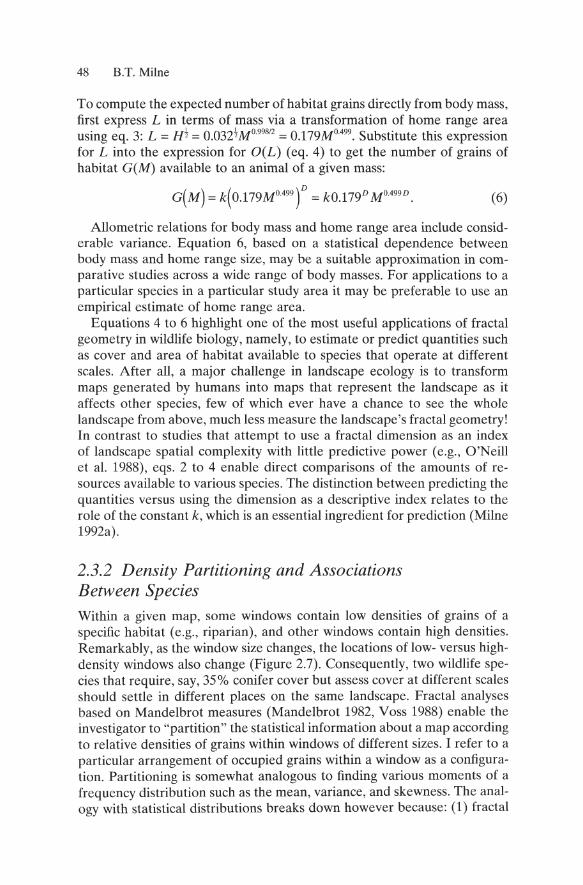
To compute the expected number of habitat grains directly from body mass, first express L in terms of mass via a transformation of home range area using eq. 3: L = Ht = O.032tM099812 = O.179M°.499. Substitute this expression for L into the expression for G(L) (eq. 4) to get the number of grains of habitat G(M) available to an animal of a given mass:

G(M) = k(O.179M°.499t = kO.179D M°.499D. (6)

Allometric relations for body mass and home range area include considerable variance. Equation 6, based on a statistical dependence between body mass and home range size, may be a suitable approximation in comparative studies across a wide range of body masses. For applications to a particular species in a particular study area it may be preferable to use an empirical estimate of home range area.

Equations 4 to 6 highlight one of the most useful applications of fractal geometry in wildlife biology, namely, to estimate or predict quantities such as cover and area of habitat available to species that operate at different scales. After all, a major challenge in landscape ecology is to transform maps generated by humans into maps that represent the landscape as it affects other species, few of which ever have a chance to see the whole landscape from above, much less measure the landscape's fractal geometry! In contrast to studies that attempt to use a fractal dimension as an index of landscape spatial complexity with little predictive power (e.g., O'Neill et al. 1988), eqs. 2 to 4 enable direct comparisons of the amounts of resources available to various species. The distinction between predicting the quantities versus using the dimension as a descriptive index relates to the role of the constant k, which is an essential ingredient for prediction (Milne 1992a).

2.3.2 Density Partitioning and Associations Between Species Within a given map, some windows contain low densities of grains of a specific habitat (e.g., riparian), and other windows contain high densities. Remarkably, as the window size changes, the locations of low- versus highdensity windows also change (Figure 2.7). Consequently, two wildlife species that require, say, 35% conifer cover but assess cover at different scales should settle in different places on the same landscape. Fractal analyses based on Mandelbrot measures (Mandelbrot 1982, Voss 1988) enable the investigator to "partition" the statistical information about a map according to relative densities of grains within windows of different sizes. I refer to a particular arrangement of occupied grains within a window as a configuration. Partitioning is somewhat analogous to finding various moments of a frequency distribution such as the mean, variance, and skewness. The analogy with statistical distributions breaks down however because: (1) fractal


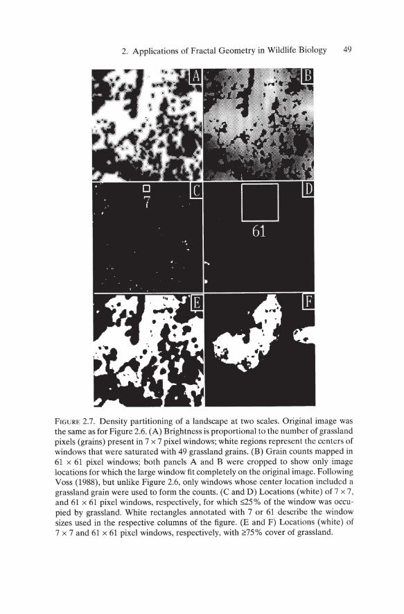
FIGURE 2.7. Density partitioning of a landscape at two scales. Original image was the same as for Figure 2.6. (A) Brightness is proportional to the number of grassland pixels (grains) present in 7 x 7 pixel windows; white regions represent the centers of windows that were saturated with 49 grassland grains. (B) Grain counts mapped in 61 x 61 pixel windows; both panels A and B were cropped to show only image locations for which the large window fit completely on the original image. Following Voss (1988), but unlike Figure 2.6, only windows whose center location included a grassland grain were used to form the counts. (C and D) Locations (white) of 7 x 7 , and 61 x 61 pixel windows, respectively, for which ::;25% of the window was occupied by grassland. White rectangles annotated with 7 or 61 describe the window sizes used in the respective columns of the figure. (E and F) Locations (white) of 7 x 7 and 61 x 61 pixel windows, respectively, with ~75% cover of grassland.

50 B.T. Milne

partitioning provides additional information about "negative moments," which describe the sparse configurations of grains (Milne 1991a), and (2) the scale dependence of each moment can be measured to learn how the geometry of sparse configurations differs from that of dense configurations (Feder 1988). Sparse configurations of grains can be thought of as "stepping stones" between higher concentrations of grains. Some landscapes contain more stepping stones than others, with implications for the connectivity between dense patches of habitat. Partitioning provides a suite of scaling exponents, one for each moment, and thus a more complete characterization of the pattern than can be had from any single dimension or exponent. In theory, the scaling exponents of all moments converge for infinite size maps but the finite extent of empirical maps makes the convergence a very special case.

In the management of pest outbreaks or of predator-prey interactions, it may be necessary to know the spatial association between host and parasite or predator and prey. In a nonfractal world, the associations can be described by a correlation coefficient between the abundances of one member of the pair and the other (Mangle and Adler 1994). However, if either or both players are fractally distributed, then the correlation between the two will change with scale (Scheuring and Riedi 1994).

It is reasonable to measure the association between a predator and a prey by focusing on the predator. Then, one can ask what the chance of finding a prey item is within a given search radius. Operationally, one centers a quadrat or window on the predator and counts the number of prey present. Replicate predators would provide a distribution of surrounding prey densities.

Measurements of the association between two species are made by scanning across a map of species 1 with a window of length L. Windows whose center location coincides with a grain containing species 1 are inspected. If any grains within the window are occupied by species 2, then the number of grains with species 1 is tallied to provide a measure of species 1 abundance, conditional on the presence of species 2 (Scheuring and Riedi 1994).

The analysis can be generalized for measurement of the fractal geometry of a given species contingent on the presence of any number of other species or environmental conditions. Specifically, the analysis involves counting the number of grains of species j = 1 that occur in windows of length L occupied by at least one grain of species j = 2,3, ... S, where S is the number of species under study; grains for species j "# 1 do not have to be in the center of the window. Each species occupies a set of points called Ii' which can be thought of as a map of all the grains that contain species j. For any given window size L there is a number of windows W(L,lt ... Is) for which species 1 is present at the center location and species 2 ... S are present in the window. At each window location i, there are nj (It 112 ... Is) grains of species 1 conditional ("I") on the other species. Since the counts


need to be divided by the total mumber of windows that satisfy the condition, the total number of grains of species 1 that satisfy the condition is n(lj1/2 . .. Is) = Lini (ltI/2 ... Is). The portion of the total at location i is Pi(lt1/2 ... is) = nl/tli2 ... Is)/n(ltI/2 ... Is)· The portions Pi(ltl/2 ... Is) have ex-plicit spatial coordinates and as such constitute a geometric measure (Morgan 1988) on the landscape. Scheuring and Riedi (1994) compute scaling exponents from the portions Pi (lt1/2 ... Is) using an ambiguous series of equations.

I compute the scaling behavior of the measures by recasting the portions in terms that enable use of an alternative expression (Voss 1988, Milne 1991a, 1992a). Since a frequency distribution can be made of the grain counts ni(ltI/2 . .. Is), I follow Voss (1988) and first compute the probability P(m,L) of observing m = ni(ltI/2 . .. Is) points in a window of length L. The values of mare <5.L 2 so Lm=! P(m,L) = 1. The fractal moments are formed:

L'

M(Lf = I,mqP(m,L), (7) k=!

which defines the qth fractal moment M(L)q. Since raising m to a high power effectively creates a large weight by which P(m,L) is multiplied, positive values of q produce moments that emphasize the contribution of densely filled windows, i.e., locations where many grains of species 1 occur with all the subsidiary species. In contrast, negative q values down weight dense windows in favor of sparse windows. Thus, q can be thought of as a tuning parameter that enables the moments to reflect selected partitions of the species distribution. As it turns out, some values of m at a fine scale produce high values of m q P(m,L) and thereby contribute a lot to the size of the moment (eq. 7). At broader scales other values of m contribute a lot but these values of m generally occur at different locations than the important m values at the fine scale. Since the moment at scale L characterizes "what the animal encounters," we conclude that animals that operate at different scales are influenced by different locations.

The qth roots of the moments increase as a power of L (Voss 1988, Milne 1991a, 1992a) according to:

/ )t/q \M(Lf =kLDq (8)

for q i= 0; for q = 0, Do is obtained from the slope of T(L) -In L where T(L) = Lm logm P(m,L). The brackets "( ) " indicate that an average has been taken. The result is an entire family of scaling exponents D q. The notion that a fractal is composed of partitions, each of which has its own scaling exponent, led to the term multifractal (Feder 1988). Scaling relations (e.g., eq. 8) are valid only when the moments increase as a power of L. It is

52 B.T. Milne

necessary to inspect doubly logarithmic graphs of the transformed qth root of the moments and L to verify the assumption of multifratality (Scheuring and Riedi 1994).

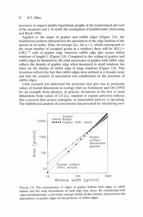
Applied to the maps of gopher and rabbit edges (Figure 2.6), the multifractal analysis characterizes the association of the edge habitats of the species at all scales. Thus, on average (i.e., for q = 1, which corresponds to the mean number of occupied grains in a window) there will be M(L) = 0.08 L 186 cells of gopher edge wherever rabbit edge also occurs within windows of length L (Figure 2.8). Compared to the scaling of gopher and rabbit edges by themselves, the joint occurrence of gopher with rabbit edge reflects the density of gopher edge when measured in small windows but takes on the density of rabbit edge in large windows (Figure 2.8). This transition reflects the fact that rabbit edges were defined at a broader scale and that the analysis of association was conditioned on the presence of rabbit edges.

Little research has addressed the processes that give rise to particular values of fractal dimensions in ecology (but see Sommerer and Ott [1993] for an example from physics). in general, deviations of the box or mass dimensions from values of 2.0 (i.e., random or regular patterns) indicate that a process that creates contagion, or nonrandom pattern, is operating. The multifractal analysis of co occurrence has potential for identifying envi-

10000

.---... Vl c 1000 .-0 I....

OJ '--"

0 (J) 100 I....

«

1 0

1 0

-- -- Gopher Geee8 Rabbit ..... Gopher AND rabbit

Rabbit pattern dominates

Gopher pattern limits density

100

gopher

Window width (grains) 1000

FIGURE 2.S. The co occurrence of edges of gopher habitat with edges of rabbit habitat and the scale dependence of each edge type alone. By considering both edges simultaneously, a new slope emerges which, in this analysis, characterizes the dependence of gopher edges on the presence of rabbit edges.


ronmental factors or species associations that regulate a given species distribution, as indicated by the novel dimension that emerged from considering the co occurrence of gopher and rabbit edges. Sole and Manrubia (1995) show that changes in the parameters of a simulation model (i.e., changes in the process rates) alter the dimensions. In this sense, the scaling behavior of any given ecological fractal could be considered diagnostic of some underlying physical or biological process that constrains the fractal to some finite subset of the landscape.

Scheuring and Riedi (1994) show how to use multifractal results to form standard X2 contingency tables to evaluate co occurrence at all scales simultaneously. Their innovation addresses concerns about finding "the" proper measurement scale for studies of species associations in spatially complex landscapes, at least for ranges of window sizes that satisfy the multifractal assumption. Simultaneous tests for association across a range of scales are possible.

2.4 Flux

Fluxes form the basis for many landscape and resource management decisions. Fluxes describe the production of forage, trace greenhouse gases such as methane, and reproductive effort expended on a landscape during the breeding season. Where nonrandom patterns or incomplete mixing of gasses occur, ecologists and wildlife biologists who extrapolate fine-scale field measurements to predict patterns and fluxes over broad regions need to incorporate the spatial heterogeneity of the landscape into the predictions. Some of the most difficult problems relate to estimating fluxes, or rates of production of matter and energy per unit area through time.

Substitution of the home range equation (eq. 3) into expressions for metabolic fluxes could be used in models of nutrient cycling rates at various scales. For example, mammals excrete N at rates (g/s):

N( M) = 3.41 X 10-6 M074 (9)

(Stahl 1962). Flux, which is the mass of N per unit area per unit time, is found by dividing N(M) by the area from which flux can occur, namely the number of habitat grains occupied by an animal of a given mass G(M), (eq. 6). Thus, the flux from an animal of mass M living on a landscape with dimension D has units gm-2s-1:

F(M) = N(M)/G(M) = 3.41 x 10-6 M0 74/( kO.179 D MOA99D)

= 3.41 x 10-6 M074-0A99D / kO.179 D. (10)

Equation 10 is simply a ratio of nitrogen loss rate N(M) divided by the grains of habitat available to the animal within its home range G(M). As

54 B. T. Milne

before (eq. 4,5,6), k is a constant derived by regression and is related to the geometry of gaps (Mandelbrot 1982), or equivalently the degree of contagion (Milne 1992a) within the landscape. Similar expressions can be derived for other emissions from animals such as methane, evaporative water (e.g., Crawford and Lasiewski 1968), and feces (Blueweiss et a1. 1978). Following the logic of eq. 10, the flux of evaporative water (Crawford and Lasiewski 1968) is:

w( M) = 4.4 X 10-4 MO.88-{)449D / kO.179 D• (11)

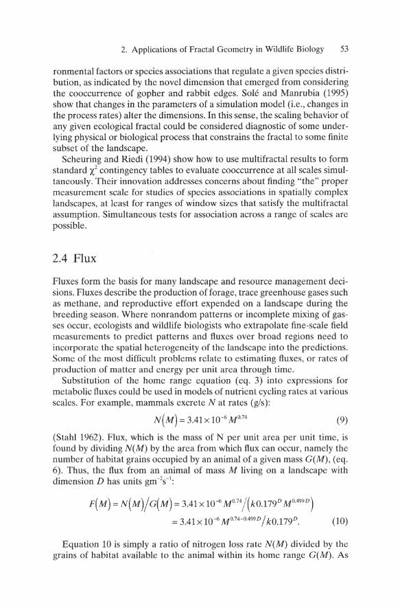
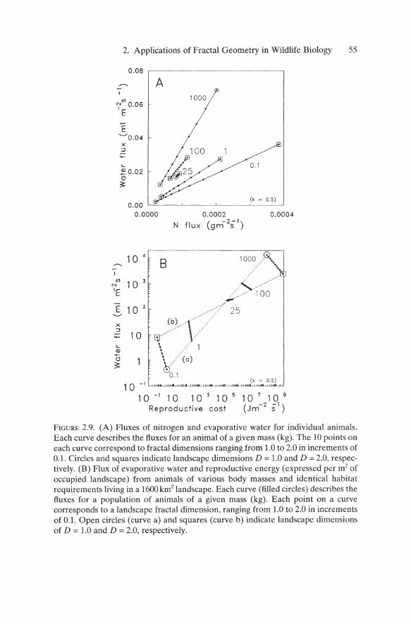
Comparisons of the per individual fluxes of N and evaporative water for mammals ranging from 0.1 to 1000kg revealed a startling interaction between the relative magnitudes of the fluxes and the fractal dimension of the landscape (Figure 2.9A). Small mammals (0.1 kg) generate relatively high N flux, compared to water flux, for landscapes of all dimensions. The ratio of N flux to water flux is lower for large mammals, reflecting the tremendous water demand of large mammals. The water conservation strategies of small mammals, combined with a preference for high N foods, such as seeds, suggests that small mammals could explain the preponderance of variation in N flux from one landscape to the next.

Interestingly, species of modest size (25 kg) display comparable fluxes for both N and water in landscapes of any dimension. Such species would be perfect generalists, performing equally well in any landscape. It is intriguing to wonder whether people "selected" goats, sheep, and swine as domestic animals (rather than rodents or elephants) because of the merits of a 25 kg beast.

The compression of the curve for 25kg animals (Figure 2.9A) reflects a mass-dependent reversal of fluxes in low- versus high-dimensional landscapes. For example, the 0.1 kg animal has a lower evaporative flux in a landscape where D = 1.0 than in a landscape with D = 2.0 (Figure 2.9A). In contrast, the highest water flux of 1000-kg species occurs at D = 1.0. Presumably the homogeneity of a D = 2.0 landscape, coupled with the lower transport costs of large animals, implies greater access to water and to cover for thermoregulation. Collectively, the ends of the curves bound a set of observable fluxes (assuming a constant value of k that would probably vary among species with different habitat requirements, even within a given landscape) .

I used an allometric expression for population density (Damuth 1981) to calculate the total flux of evaporative water and total reproductive cost (Peters 1983, p. 127, after Brody 1945) for 1600km2 1andscapes. I multiplied the per-animal reproductive cost R(M), measured in joules, by the number of females expected over the area (Figure 2.9B). As for individual fluxes, landscape heterogeneity interacts with body mass such that large animals have the highest per-landscape reproductive costs on the most homogeneous landscapes (D = 2.0), possibly due to intraspecific competition related to overlapping home ranges. The reverse is true for small animals. The body


0 .08

,--..

1

A Ul I' 0.06 E

E '-'0 .04 x :J

'-20.02 o 3:

"I Ul

N

'E

E x ::J

'-CIl -0

3:

0 .00 0.0000

10 4

10 3

10 2

10

B

1000

0.1

(k = 0.5)

0.0002 0.0004

N flux (gm-2S- 1)

.,;... f

/ ,' 25

(k = 0.5) 1 0 -1 L...Lu.."'-'-w"'--'-u"""--w"""'-'.uwoLLtimL-,-,"",LLum'-"""'--".uuoLuJ

1 0 -1 1 0 1 0 3 1 0 5 1 0 7 1 0 9

Reproductive cost (Jm- 2 51)

FIGURE 2.9. (A) Fluxes of nitrogen and evaporative water for individual animals. Each curve describes the fluxes for an animal of a given mass (kg). The 10 points on each curve correspond to fractal dimensions ranging from 1.0 to 2.0 in increments of 0.1. Circles and squares indicate landscape dimensions D = 1.0 and D = 2.0, respectively. (B) Flux of evaporative water and reproductive energy (expressed per m2 of occupied landscape) from animals of various body masses and identical habitat requirements living in a 1600 km2 landscape. Each curve (filled circles) describes the fluxes for a population of animals of a given mass (kg). Each point on a curve corresponds to a landscape fractal dimension, ranging from 1.0 to 2.0 in increments of 0.1. Open circles (curve a) and squares (curve b) indicate landscape dimensions of D = 1.0 and D = 2.0, respectively.

56 B.T. Milne

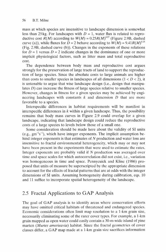
mass at which species are insensitive to landscape dimension is somewhat less than 25kg. For landscapes with D = 1, water flux is related to reproductive cost R(M) according to W(M) = O.25R(M)057 (Figure 2.9B, dashed curve (a)), while fluxes for D = 2 behave according to W(M) = 9.41R(M)025 (Fig. 2.9B, dashed curve (b)). Changes in the exponents of these relations for D = 1 versus D = 2 indicate changes in the dominance of one or more implicit physiological factors, such as litter mass and total reproductive cost.

The dependence between body mass and reproductive cost argues strongly for the preservation of large tracts of land to support the reproduction of large species. Since the absolute costs to large animals are higher than costs to smaller species in landscapes of all dimensions (1 < D < 2), it is untenable to argue that wise landscape design (i.e., design that manipulates D) can increase the fitness of large species relative to smaller species. However, changes in fitness for a given species may be achieved by engineering landscapes with constants k and dimension D that are more favorable to a species.

Interspecific differences in habitat requirements will be manifest in interspecific differences in k within a given landscape. Thus, the possibility remains that body mass curves in Figure 2.9 could overlap for a given landscape, indicating that landscape design could reduce the reproductive costs of a large species to levels below those of a small one.

Some consideration should be made here about the validity of SI units (e.g., gm-2s-1), which have integer exponents. The implicit assumption behind integer exponents is that estimates of N production and water loss are insensitive to fractal environmental heterogeneity, which mayor may not have been present in the experiments that were used to estimate the rates. Integer exponents are probably valid if N production was averaged over time and space scales for which autocorrelation did not exist, i.e., variation was homogeneous in time and space. Pennycuick and Kline (1986) proposed that units of measure be superscripted by the appropriate dimension to account for the effects of fractal patterns that are at odds with the integer dimensions of SI units. Assuming homogeneity during calibration, eqs. 10 and 11 suffice to incorporate spatial heterogeneity of the landscape.

2.5 Fractal Applications to GAP Analysis

The goal of GAP analysis is to identify areas where conservation efforts may have omitted critical habitats of threatened and endangered species. Economic considerations often limit map resolution to a l-km grain size, necessarily eliminating some of the rarer cover types. For example, a l-km grain mapped as open water could easily contain a 30-m-wide island of pine marten (Murtes amerieavia) habitat. Since the fractal geometries of cover classes differ, a GAP map made at a l-km grain size sacrifices information


about some classes more than others. Moreover, the risk that a given 1-km grain omits a particular class depends on the multifractal association between the mapped class and the omitted classes.

There are many ways to aggregate fine-scale maps to coarse scales. Some of the best understood methods are renormalization methods (Gould and Tobochnik 1988, Cresswick et al. 1992, Milne and Johnson 1993) which involve aggregation of 2 x 2 blocks of grains. A block is converted into a single grain if the set of occupied grains within it satisfy a rule chosen by the investigator. For example, the "percolation" rule (Gould and Tobochnik 1988) results in an occupied block if at least two occupied grains are adjacent vertically (Fig. 2.10A). In cases that involve multiple cover classes on random maps, the minority classes are lost upon aggregation because they make up less than 61 % of the total cover on the map (Gould and Tobochnik 1988). Autocorrelation within actual landscapes results in similar effects at coverages not equal to 61 %. Some rules eliminate classes below other critical densities (e.g., 50% for the majority rule, Turner et al. 1989). In contrast, the similarity dimension rule preserves cover density by maintaining a constant fractal dimension of a selected class (Milne and Johnson 1993 Figures 2.10, 2.11).

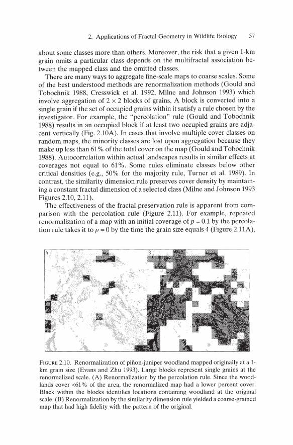
The effectiveness of the fractal preservation rule is apparent from comparison with the percolation rule (Figure 2.11). For example, repeated renormalization of a map with an initial coverage of p == 0.1 by the percolation rule takes it to p == 0 by the time the grain size equals 4 (Figure 2.11A),

FIGURE 2.10. Renormalization of pinon-juniper woodland mapped originally at a 1-km grain size (Evans and Zhu 1993). Large blocks represent single grains at the renormalized scale. (A) Renormalization by the percolation rule. Since the woodlands cover <61 % of the area, the renormalized map had a lower percent cover. Black within the blocks identifies locations containing woodland at the original scale. (B) Renormalization by the similarity dimension rule yielded a coarse-grained map that had high fidelity with the pattern of the original.

58 B.T. Milne

"0 Q)

1.0

g-0.8 (,) (,)

o 0.. 0 . 6 o E

0 0 .4

c o 1: 0.2 o

Q..

"0 Q)

g-0 .8 (,) (,)

o 0..0 .6 o E

'0 0 .4

c o 1: 0.2 o

Q..

0.0

A

Exten t: 1024

B

Extent: 1024

10 100 1000 Grain size

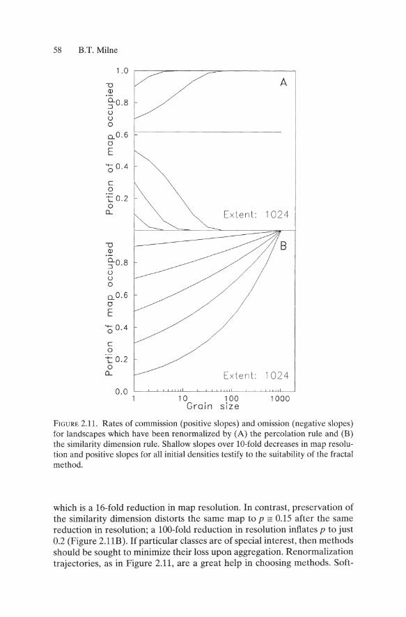
FIGURE 2.11. Rates of commission (positive slopes) and omission (negative slopes) for landscapes which have been renormalized by (A) the percolation rule and (B) the similarity dimension rule. Shallow slopes over lO-fold decreases in map resolution and positive slopes for all initial densities testify to the suitability of the fractal method.

which is a l6-fold reduction in map resolution. In contrast, preservation of the similarity dimension distorts the same map to p == 0.15 after the same reduction in resolution; a 100-fold reduction in resolution inflates p to just 0.2 (Figure 2.11B). If particular classes are of special interest, then methods should be sought to minimize their loss upon aggregation. Renormalization trajectories, as in Figure 2.11, are a great help in choosing methods. Soft-


ware and a tutorial for renormalization and other fractal analyses are available at: (http://sevilleta.unm.edu/-bmilne/frac/clara/clarat.html).

2.6 Species Area Relations Are Fractal

The classic species area curves, that describe the number of species per area, form the basis of major theories about the distribution and abundance of organisms (Preston 1962, MacArthur 1972, Rosenzweig 1995). The species area relation is an essential tool for estimating biodiversity. Interestingly, the species area relation can be expressed readily as a fractal scaling law by taking the square root of area to obtain a length scale.

In particular, the classic relation between the number of species Sand island area A is:

S = CA' (12)

and includes the exponent z. Taking the square root of area gives

S = e( Al /2 r = CA Z/2 , (13)

which can be rewritten in terms of length:

S = eLY (14)

for which y = z12. Since S is an "affine function" (Barnsely 1988), it is inappropriate to call ya fractal dimension. It is, however, a scaling exponent, and a dimension could be obtained from studies of the autocorrelation or semivariance of S (Milne 1991a). Consequently, empirical z values may be explained at least partly as a consequence of life on fractal terrain, such as islands. For instance, if an observation window is centered on an island or continent, increasing window sizes encompass all of the island until they ultimately include some of the surrounding water where terrestrial species are absent. This is similar to a Scheuring and Riedi (1994) analysis of one species contingent on the presence of one or more other species. Here however, the "species" of interest is the set of all species (which are counted to give S) and the land is analogous to "other species." Since terrestrial species must occur on land, S is implicitly conditioned on the presence of terra firma. With increasing window size, the absence of land beyond the island boundary is the constraint that limits S. Since the land boundary is fractal (Figure 2.2), its dimension should dominate the scaling exponent of the species area curve when the window size is greater than roughly half the island diameter and less than or equal to the width of the island. Thus, expressing the species area curve as a fractal scaling relation emphasizes the ultimate constraint of land mass on species richness. This, of course, is the intention of the classical species area curve, but the fractal geometry of the land is generally ignored (but see Scheuring 1991).

60 B.T. Milne

To incorporate the geographic complexity of islands, I compute the box fractal dimension of an island by making a map of it, overlaying a grid of boxes of length L, and then counting the number of grid cells that contain any part of the island. For box sizes smaller than the island width, the number of boxes that contain parts of the island N(L) is:

N(L)=kC Db (15)

where Db is the "box" dimension (Voss 1988). The exponent is negative because the number of boxes decreases as the box size increases. Multiplying N(L) by the area of the box (L2) gives the area at scale L: A(L) = N(L)L2 = kL2- Db. Since Db is <2, the apparent area increases with L. This expression for area can be substituted in eq. 12 to incorporate the geometry of the island:

S(L) = c( kL2-Db r. (16)

Throughout the history of the study of species-area relations, investigators have neglected to use eq. 15 to partial out the scale dependence of island area, which is equivalent to rewriting eq. 16 as

S(L) = ckzLz(Z-Db) = ckzA z-(ZDb)/2, (17)

in which the dimension of the island is confounded by the species area exponent z. Equation 16 eliminates ambiguity about the scale at which the island area was measured and enables estimates of S(L) from various islands to be controlled, or normalized, for L. Normalization entails expressing the area of each island at a common L. For example, given the scaling relations for two islands and areas computed at arbitrary scales (km2),

Island A: AA(L) = 0.51L2-16 ; AA(I) = 0.51km2 for L = 1

Island B: A8(L) = 0.32L2- L2 ; A8(2) = 0.55km 2 for L = 2,

it is possible to express the area of the small Island A at the same measurement scale as Island B; AA(2) = 0.51(22 - 16) = 0.67 km2. Expressed at the same scale, Island A is larger than B, because the higher fractal dimension and constant conspire to provide more island area as the resolution is increased. Normalizing island area across all islands should disentangle the exponent in the classic species-area relation from the implicit exponent of eq. 14. If whole archipelagos are to be treated as study units, then the box dimension of each archipelago, coupled with species richness estimates for the archipelago, would enable tests of Scheuring's (1991) hypothesis that species richness is controlled by energy expenditures that scale with body mass raised to the 3/4 power. His accounting for surface roughness on


islands could also be combined with the above suggestion that the box dimension is related to the classic species area curve.

It should not be surprising that species richness is disproportionately high in the Andes of South America where rough terrain creates islands of habitat with low box dimensions. In the extremes, when habitat is confined to jagged peaks that create patches with Db - 1, eq. 16 becomes approximately S(L) = c(kLY, whereas smooth, round patches with D - 2 imply S(L) = c(kLoy = ck', which should be less diverse. Under this hypothesis, rough terrain partitions habitat into smaller units and fosters diversification over evolutionary time. Connectivity or homogeneity, which are maximal when island area scales as L2, would tend to enable competitive dominants to eliminate other species or would allow genetic introgression to disrupt locally adapted genotypes, thereby reducing evolutionary potential and diversity.

2.7 Scaling of Population Changes

Much has been written about the scale dependence of fractal changes through time, such as variation in river flows and sunspots (Hurst 1951, Mandelbrot and Wallis 1969, Feder 1988). Temporal fractals require different quantitative approaches than those used for coastlines and binary maps (Mandelbrot 1982, Voss 1988, Milne 1991a). Limited applications in ecology (Sole et al. 1992) provide one reliable method of characterizing fluctuations in population sizes across a range of time scales so as to identify periods of scale dependence and possible relations with fractal environmental variables.

For example, I hypothesized that the EI Nino Southern Oscillation Phenomenon (ENSO), which is widely recognized as an historically important perturbation of foodwebs in the Pacific Ocean, would exhibit scaling behavior similar to fluctuations in pelican population sizes. The ENSO fluctuations are characterized by the Southern Oscillation Index (SOl), which is the pressure differential between Darwin, Australia and Tahiti. Persistent low values of the index presage an EI Nino event that disrupts ocean currents, upwelling, and the delivery of nutrients to the foodchain. Presumably, collapse of the fish populations during EI Nino cascades up the foodchain to affect pelican population sizes. If pelican fluctuations are indeed tied to ENSO, then both should exhibit similar scaling behavior.

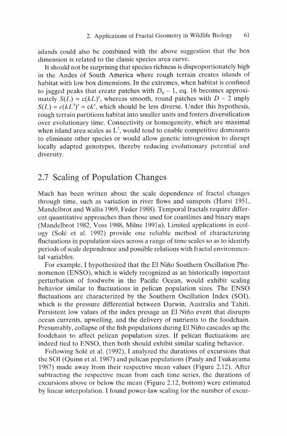
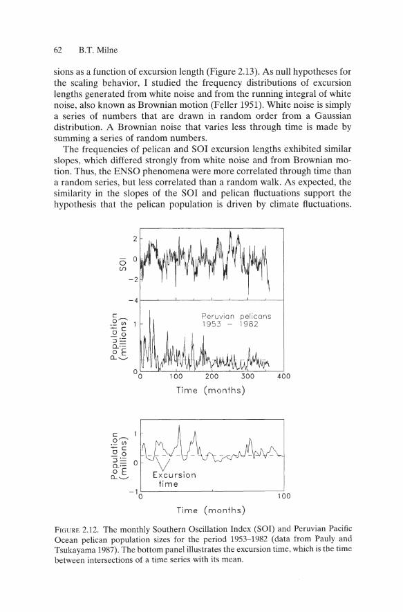
FOllowing Sole et al. (1992), I analyzed the durations of excursions that the SOl (Quinn et al. 1987) and pelican populations (Pauly and Tsukayama 1987) made away from their respective mean values (Figure 2.12). After subtracting the respective mean from each time series, the durations of excursions above or below the mean (Figure 2.12, bottom) were estimated by linear interpolation. I found power-law scaling for the number of excur-

62 B.T. Milne

sions as a function of excursion length (Figure 2.13). As null hypotheses for the scaling behavior, I studied the frequency distributions of excursion lengths generated from white noise and from the running integral of white noise, also known as Brownian motion (Feller 1951). White noise is simply a series of numbers that are drawn in random order from a Gaussian distribution. A Brownian noise that varies less through time is made by summing a series of random numbers.

The frequencies of pelican and Sal excursion lengths exhibited similar slopes, which differed strongly from white noise and from Brownian motion. Thus, the ENSO phenomena were more correlated through time than a random series, but less correlated than a random walk. As expected, the similarity in the slopes of the Sal and pelican fluctuations support the hypothesis that the pelican population is driven by climate fluctuations.

2

o 0 lfl

c 0---..

._ III

..... c o 0

:i=-= 0..:= o E

0... "--'

c .~~ ..... c ~o :J::: 0..:= 0 o E

0... "--'

Peruvian pelica ns 1953 - 1982

Time (months)

Time (months)

400

100

FIGURE 2.12. The monthly Southern Oscillation Index (SOl) and Peruvian Pacific Ocean pelican population sizes for the period 1953-1982 (data from Pauly and Tsukayama 1987). The bottom panel illustrates the excursion time, which is the time between intersections of a time series with its mean.


1000

>- 100 (J

c (j)

::::l 0- 10 (j) L

l.J....

0 . 1

Whi t e n Oise

•• ----- ---.-0 Brown ian --- 0

motion

~ Pelicans 0 0 000 SOl

10

Excursion time (months)

FIGURE 2.13. Scaling of the frequencies of excursion times for white noise, Brownian motion, the monthly Southern Oscillation Index (SOl), and pelican population sizes.

This method could be applied to other observations to test for the effects of constraints that govern the fluctuations .

2.8 Landscape Design

Natural resource management entails landscape planning and design. Although the use of fractals to make striking images of landscapes, terrain, and vegetation (Mandelbrot 1982, Barnsley 1988) provides visually convincing arguments that fractal geometry has uses in ecology and wildlife biology, a lack of theoretical basis for the ecological benefits of fractal designs has hampered their application. Milne (1991b) explained the use of iterated function systems (Barnsley 1988) to generate fractal designs that are aesthetically pleasing, naturalistic, and easy to generate. Thus, it is conceivable that patterns such as clearcuts, plantations, and parklands could be manipulated based on fractal designs with potential benefits to wildlife because the designs are self-similar, as are patterns in nature. Morse et a1. (1985) suggested that fractal environments support many species by accommodating a wide range of body sizes, each of which perceives the environment at different scales. Theory predicts that fractal landscape patterns of different dimensions affect ecological processes (Fig. 2.9) . Thus, landscapes designed to have a given dimension and the associated self-

64 B. T. Milne

similarity across a range of scales could increase the reproductive success of a targeted species of reduce that of a pest.

2.9 Conclusions

A wealth of alternative fractal models exist to aid in the characterization of complex landscape patterns. Species abundances, habitat patterns, coastline geometries, fluxes, cartographic estimation, landscape design, and population fluctuations all are amenable to fractal analysis. In this chapter I focused on selected applications that may typify the types of problems encountered in wildlife biology. Existing allometric relations (Peters 1983) formed the basis for analyses of energy, water, and nutrient fluxes in landscapes with various dimensions. This application illustrates how new fractal relations can be generated for particular problems.

An underlying theme throughout this chapter is that fractal geometry is most effective when used to predict quantities such as habitat area, coastline length, and fluxes. Many papers in the field of landscape ecology have emphasized the measurement of one or several types of fractal dimension. These studies often stop short of prediction, having halted at description. There are, indeed, instances when a dimension forms a stringent index that, if equal to a theoretical value, is diagnostic of fundamental dynamical processes, e.g., Feder (1988), Sommerer and Ott (1993). However, use of fractal dimensions without explicit a priori expected values ranks as one of the weakest uses.

Fractal power laws are diagnostic of one or more processes that act in a consistent fashion over a range of scales (Krummel et a1. 1987). However, such laws generally apply over a finite range of scales (Fig. 2.5), and other forms of scale dependence may apply, such as exponential relations. Care is needed, in the form of graphical inspection of the measured quantities as a function of scale, to evaluate the appropriateness of a fractal scaling law for a given application. Such scrutiny is absolutely necessary for multifractal applications (eq. 8) and for studies of co-occurrence, especially when characterizing the scale dependence of sparse occurrences, i.e., for q < O.

Finally, fractal geometry provides highly effective tools to address the complexity of nature. The regular statistical behavior of complex patterns provides quantitative insights into what otherwise are bewildering irregularities that confound many of the traditional approaches in ecology, wildlife biology, and management.

2.10 Summary

Species use resources at different scales by virtue of allometric variation in home range area, metabolic rate, and movement speeds. Consequently, fractal distributions of habitat and resources imply that a given landscape


represents effectively different resource patterns for each species. Assessments of resource availability at multiple scales are needed to predict the coexistence of species, to estimate effective habitat area, and to characterize the ways in which species respond to spatial complexity. The fundamentals for such assessments include the notion of scale dependence, the measurement of fractal dimensions, and visualizations of resource density at many scales. This chapter introduced a range of insights possible from multiscale analyses of resource patterns. Specific applications to wildlife biology included estimation of bald-eagle nest density along a coastline; estimation of red-cockaded woodpecker habitat area for the southern United States; models of the fluxes of water, nitrogen, and reproductive energy costs for herbivorous mammals living on fractal landscapes; modification of the classic species-area relation to accommodate the fractal geometry of islands; aggregation of fine-scale maps to coarse resolution as in GAP analysis; analyses of pelican population changes in relation to fluctuations in the El Nino Southern Oscillation phenomenon; and visualization of habitat edges at multiple scales. Fractal analyses in wildlife biology simultaneously provide statistical and spatial information with which to assess habitat availability and to guide management decisions.

2.11 Acknowledgments. Many thanks to John Bissonette for motivating this work and to Alan Johnson for suggesting the pelican study. The redcockaded woodpecker range map was obtained from the National Biological Service via http://www.im.nbs.gov/bbs/htmra/h3950ra.html. Yeulong Yang provided a constructive critique of the manuscript. Support was provided by the NSF (grants BSR-9058136 and BSR-9107339) and the Electric Power Research Institute. Sevilleta LTER publication no. 94.

2.12 References Allee, W.e. 1931. Animal aggregations: A study in general sociology. University of

Chicago Press, Chicago, Illinois, USA. Allen, T.F.H., and T.B. Starr. 1982. Hierarchy. University of Chicago Press, Chi

cago, Illinois, USA. Allen, T.F.H., and T.W. Hoekstra. 1992. Toward a unified ecology. Columbia Uni

versity Press, New York, New York, USA. Barnsley, M. 1988. Fractals everywhere. Academic Press, New York, New York,

USA. Blueweiss, L., H. Fox, V. Kudzma, D. Nakashima, R. Peters, and S. Sams. 1978.

Relationships between body size and some life history parameters. Oecologia (Berlin) 37:257-272.

Brody, S. 1945. Bioenergetics and growth. Reinhold Publishing Company, Baltimore, Maryland, USA.

Brown, J.H. 1995 Macroecology. University of Chicago Press, Chicago, Illinois, USA.

66 B.T. Milne

Brown, J.H., P.A Marquet, and M.L. Taper. 1993. Evolution of body size: consequences of an energetic definition of fitness. American Naturalist 142:573-584.

Burrough, P.A 1986. Principles of geographical information systems for land resources. Assessment. Clarendon Press, Oxford, UK.

Clements, F.E. 1905. Research methods in ecology. The University Publishing Company, Lincoln, Nebraska USA

Crawford, E.c. Jr., and RC. Lasiewski. 1968. Oxygen consumption and respiratory evaporation of the emu and rhea. Condor 70:333-339.

Cressie, N.AC. 1991. Statistics for spatial data. J. Wiley & Sons Inc., New York, New York, USA

Cresswick, RJ., H.A Farach, and c.P. Poole, Jr. 1992. Introduction to renormalization group methods in physics. J. Wiley & Sons Inc., New York, New, Yrok, USA

Damuth, J. 1981 Population size and body size in mammals. Nature 290:699-700. Delcourt, H.R, and P.A Delcourt. 1988. Quaternary landscape ecology: relevant

scales in space and time. Landscape Ecology 2:23-44. Deutsch, C.V., and AG. Journel. 1992. GSLIB: Geostatistical software library and

user's guide. Oxford University Press, Oxford, UK. Erickson, RO. 1945. The Clematis fremontii var. Riehlii population in the Ozarks.

Annals of the Missouri Botanical Garden 32:413-460. Evans, D.L., and Z. Zhu. 1993. A VHRR for forest mapping: national applications

and global implications. p. 76-79 in A Lewis, editor. Looking to the future with an eye on the past: proceedings of the 1993 ACMS/ASPRS. American Society of Photogrammetry and Remote Sensing.

Feder, J. 1988. Fractals. Plenum Press, New York, New York, USA Feller, W. 1951. The asymptotic distribution of the range of sums of independent

random variables. Annals of Mathematical Statistics 22:427. Forman, RT.T. 1995. Land mosaics. Cambridge University Press. Cambridge, UK. Frank, D.A, and R.S. Inouye. 1994. Temporal variation in actual evapo

transpiration of terrestrial ecosystems: patterns and ecological processes. Journal of Biogeography 21:401-411.

Gould, H., and J. Tobochnik. 1988. An introduction to computer simulation methods: applications to physical systems. Part 2. Addison-Wesley Publishing Company, Reading, Massachusetts, USA

Grassberger, P., and 1. Procaccia. 1983. Measuring the strangeness of strange attractors. Physica D 9:189-208.

Gupta, V.K., and E.D. Waymire. 1989 Statistical self-similarity in river networks parameterized by elevation. Water Resources Research 25:463-476.

Harestad, AS., and F.L. Bunnell. 1979. Home range and body weight: A reevaluation. Ecology 60:389-402.

Holling, C.S. 1992. Cross-scale morphology, geometry and dynamics of ecosystems. Ecological Monographs 62:447-502.

Hurlbert, S.H. 1984. Pseudoreplication and the design of ecological field experiments. Ecological Monographs 54:187-211.

Hurst, H.E. 1951. Long-term storage capacity of reservoirs. Transactions of the American Society Civil Engineers 116:770-808.

Johnson, A.R, B.T. Milne, and J.A Wiens. 1992. Diffusion in fractal landscapes: Simulations and experimental studies of Tenebrionid beetle movements. Ecology 73:1968-1983.


Kauffman, S.A 1993. The origins of order. Oxford University Press, Oxford, UK.

Keitt, T.R., and A.R Johnson. 1995. Spatial heterogeneity and anomalous kinetics: Emergent patterns in diffusion-limited predator-prey interactions. Journal of Theoretical Biology 172:127-139.

Krummel, J.R., RH. Gardner, G. Sugihara, RV. O'Neill, and P.R Coleman. 1987. Landscape pattern in a disturbed environment. Oikos 48:321-324.

Levin, S.A 1992. The problem of pattern and scale in ecology. Ecology 73:1942-1968.

Loehle, c., and B.-L. Li. 1996. Statistical properties of ecological and geologic fractals. Ecological Modelling 85:271-284.

MacArthur, RH. 1972. Geographical ecology. Princeton University Press, Princeton, New Jersey, USA

Magnuson, J.J. 1990. Long-term ecological research and the invisible present. BioScience 40:495-501.

Mandelbrot, B.B. 1982. The fractal geometry of nature. W.R. Freeman and Co., New York, New York, USA

Mandelbrot, B.B., and J.R Wallis. 1969. Some long-run properties of geophysical records. Water Resources Research 5:321-340.

Mangel, M., and F.R Adler. 1994. Construction of multidimensional clustered patterns. Ecology 75:1289-1298.

Milne, B.T. 1991a. Lessons from applying fractal models to landscape patterns. Pp. 199-235 in M.G. Turner, and RH. Gardner, editors. Quantitative methods in landscape ecology. Springer-Verlag, New York, New York, USA

Milne, B.T. 1991b. The utility of fractal geometry in landscape design. Landscape and Urban Planning 21:81-90.

Milne, B.T. 1992a. Spatial aggregation and neutral models in fractal landscapes. American Naturalist 139:32-57.

Milne, B.T. 1992b. Indications of landscape condition at many scales. Pp. 883-895 in D.H. McKenzie, D.E. Hyatt, and V.J. McDonald, editors. Ecological indicators. Vol. 2. Elsevier Applied Science, London, UK and New York, New York, USA

Milne, B.T. 1993. Pattern analysis for landscape evaluation and characterization. Pp. 131-143 in M.E. Jensen, and P.S. Bourgeron, compilers. Ecosystem management: principles and applications. United States Department of Agriculture, Forest Service Pacific Northwest Research Station General Technical Report PNWGTR-318. Portland, Oregon, USA

Milne, B.T., and RT.T. Forman. 1986. Peninsulas in Maine: woody plant diversity, distance, and environmental patterns. Ecology 67:967-974.

Milne, B.T., K. Johnston, and RT.T. Forman. 1989. Scale-dependent proximity of wildlife habitat in a spatially-neutral Bayesian model. Landscape Ecology 2:101-110.

Milne, B.T., M.G. Turner, J.A Wiens, and AR Johnson. 1992. Interactions between the fractal geometry of landscapes and allometric herbivory. Theoretical Population Biology 41:337-353.

Milne, B.T., and AR Johnson. 1993. Renormalization relations for scale transformation in ecology. Pp. 109-128 in RH. Gardner, editor. Some mathematical questions in biology: predicting spatial effects in ecological systems. American Mathematical Society, Providence, Rhode Island, USA

68 B.T. Milne

Milne, B.T., AR Johnson, T.H. Keitt, e.A Hatfield, J.L. David, and P. Hraber. 1996. Detection of critical densities associated with pifton-juniper woodland ecotones. Ecology 77:805-821.

Morgan, F. 1988. Geometric measure theory. Academic Press. New York, New York, USA

Morse, D.R, J.H. Lawton, M.M. Dodson, and M.H. Williamson. 1985. Fractal dimension of vegetation and the distribution of arthropod body lengths. Nature 314:731-734.

Niklas, K.J. 1994. Plant allometry: the scaling of form and process. University of Chicago Press, Chicago, Illinois, USA

O'Neill, RV., J.R Krummel, RH. Gardner, G. Sugihara, B. Jackson, D.L. DeAngelis, B.T. Milne, M.G. Turner, B. Zygmunt, S.W. Christensen, V.H. Dale, and RL. Grahm. 1988. Indices of landscape pattern. Landscape Ecology 1:153-162.

Palmer, M.W. 1988. Fractal geometry: a tool for describing spatial patterns of plant communities. Vegetatio 75:91-102.

Pauly, D., and I. Tsukayama, editors. 1987. The Peruvian anchoveta and its upwelling ecosystem: three decades of change. Instituto de Mar del Peru, Callao, Peru.

Peitgen, H.-O., and D. Saupe. 1988. The science of fractal images. Springer-Verlag, New York, New York, USA

Pennycuick, e.J., and Kline, N.e. 1986. Units of measurement for fractal extent, applied to the coastal distribution of bald eagle nests in the Aleutian Islands, Alaska. Oecologia 68:254-258.

Peters, RH. 1983. The ecological implications of body size. Cambridge University Press, Cambridge, UK.

Pielou, E.e. 1977. Mathematical ecology. J. Wiley & Sons, New York, New York, USA

Plotnick, RE., and M.L. McKinney. 1993. Ecosystem organization and extinction dynamics. Palios 8:202-212.

Preston, F.A 1962. The canonical distribution of commonness and rarity, Part I. Ecology 43:185-215, 431-32.

Pulliam, H.R, and B.J. Danielson. 1991. Sources, sinks, and habitat selection: a landscape perspective in population dynamics. American Naturalist 137:S50-S60.

Quinn, W.H., V.T. Neal, and S.E. Antunez de Mayolo. 1987. El Nifto over the past four and a half centuries. Journal Geophysical Research 92:14449-14461.

Richardson, L.F. 1960. Statistics of deadly quarrels. E.Q. Wright and e.e. Lienau, editors. Boxwood Press, Pacific Grove, California, USA

Robards, F.e., and J.I. Hodges. 1976. Observations from 2760 bald eagle nests in southeast Alaska: progress report 1969-1976. United States Department of the Interior, Fish and Wildlife Service, Eagle Management Study. Juneau, Alaska, USA

Root, T. 1988. Energy constraints on avian distributions and abundances. Ecology 69:330-339.

Rosenzweig, M.L. 1995. Species diversity in space and time. Cambridge University Press, Cambridge, Massachusetts, USA

Rossi, RE., D.J. Mulla, AG. Journel, and E.H. Franz. 1992. Geostatistical tools for modelling and interpreting ecological dependence. Ecological Monographs 62:277-314.


Scheuring, I. 1991. The fractal nature of vegetation and the species-area relation. Theoretical Population Biology 39:170-177.

Scheuring, I., and RH. Riedi. 1994. Application of multifractals to the analysis of vegetation pattern. Journal of Vegetation Science 5:489-495.

Schneider, D.C. 1994. Quantitative ecology: spatial and temporal scaling. Academic Press, San Diego, California, USA.

Senft, RL. , M.B. Coughenour, D.W. Bailey, L.R Rittenhouse, O.E. Sala, and D.M. Swift. 1987. Large herbivore foraging and ecological hierarchies. BioScience 37:789-799.

Simpson, G.G. 1964. Species density of North American recent mammals. Systematic Zoology 13:57-73.

Sole, RV., D. L6pez, M. Ginovart, and J. Valls. 1992. Self-organized criticality in Monte Carlo simulated ecosystems. Physics Letters A 172:56-61.

Sole, RY., and S.c. Manrubia. 1995. Are rainforests self-organized in a critical state? Journal of Theoretical Biology 173:31-40.

Sommerer, J.c., and E. Ott. 1993. Particles floating on a moving fluid: a dynamically comprehensible physical fractal. Science 259:335-339.

Spalinger, D.E., and N.T. Hobbs. 1992. Mechanisms of foraging in mammalian herbivores: new models of functional response. American Naturalist 140:325-348.

Stahl, W.R 1962. Similarity and dimensional methods in biology. Science 137:205-212.

Tilman, D., and D. Wedin. 1991. Oscillations and chaos in the dynamics of a perennial grass. Nature 353:653-655.

Turcotte, D.L. 1992. Fractals and chaos in geology and geophysics. Cambridge University Press, Cambridge, UK.

Turner, M.G., RV. O'Neill, RH. Gardner, and B.T. Milne. 1989. Effects of changing spatial scale on the analysis of landscape pattern. Landscape Ecology 3:153-162.

Urban, D.L., RV. O'Neill, and H.H. Shugart. 1987. Landscape ecology. BioScience 37:119-127.

Voss, RF. 1988. Fractals in nature: from characterization to simulation. Pp. 21-70 in H.-a. Peitgen and D. Saupe, editors. The science of fractal images. SpringerVerlag, New York, New York, USA.

Wiens, J.A. 1989. Spatial scaling in ecology. Functional Ecology 3:383- 397. Yamamura, N. 1976. A mathematical approach to spatial distribution and temporal

succession in plant communities. Bulletin of Mathematical Biology 38:517-526.

wildlife and landscape ecology || applications of fractal geometry in wildlife biology

Documents