why should statisticians be interested in artificial ... · why should statisticians be interested...

Why Should Statisticians Be Interested inArtificial Intelligence?1

Glenn Shafer 2

Statistics and artificial intelligence have much in common. Both disciplines are concernedwith planning, with combining evidence, and with making decisions. Neither is an empiricalscience. Each aspires to be a general science of practical reasoning. Yet the two disciplineshave kept each other at arm's length. Sometimes they resemble competing religions. Each isquick to see the weaknesses in the other's practice and the absurdities in the other's dogmas.Each is slow to see that it can learn from the other.

I believe that statistics and AI can and should learn from each other in spite of theirdifferences. The real science of practical reasoning may lie in what is now the gap betweenthem.

I have discussed elsewhere how AI can learn from statistics (Shafer and Pearl, 1990). Here,since I am writing primarily for statisticians, I will emphasize how statistics can learn from AI. Iwill make my explanations sufficiently elementary, however, that they can be understood byreaders who are not familiar with standard probability ideas, terminology, and notation.

I begin by pointing out how other disciplines have learned from AI. Then I list some specificareas in which collaboration between statistics and AI may be fruitful. After these generalities, Iturn to a topic of particular interest to me—what we can learn from AI about the meaning andlimits of probability. I examine the probabilistic approach to combining evidence in expertsystems, and I ask how this approach can be generalized to situations where we need to combineevidence but where the thorough-going use of numerical probabilities is impossible orinappropriate. I conclude that the most essential feature of probability in expert systems—thefeature we should try to generalize—is factorization, not conditional independence. I show howfactorization generalizes from probability to numerous other calculi for expert systems, and Idiscuss the implications of this for the philosophy of subjective probability judgment.

This is a lot of territory. The following analytical table of contents may help keep it inperspective.

Section 1. The Accomplishments of Artificial IntelligenceHere I make the case that we, as statisticians, can learn from AI.

Section 2. An Example of Probability PropagationThis section is most of the paper. Using a simple example, I explain how probability

1This is the written version of a talk at the Fifth Annual Conference on Making Statistics Teaching More Effectivein Schools of Business, held at the University of Kansas on June 1 and 2, 1990.2Glenn Shafer is Ronald G. Harper Distinguished Professor, School of Business, University of Kansas, Lawrence,Kansas 66045. Research for this paper was partially supported by National Science Foundation grant IRI-8902444.The author would like to thank Paul Cohen, Pierre Ndilikilikesha, Ali Jenzarli, and Leen-Kiat Soh for comments andassistance.

2

judgments for many related events or variables can be constructed from local judgments(judgments involving only a few variables at a time) and how the computations tocombine these judgments can be carried out locally.

Section 3. Axioms for Local ComputationIn this section, I distill the essential features of the computations of the previous section

into a set of axioms. These axioms apply not only to probability, but also to other calculi,numerical and non-numerical, that have been used to manage uncertainty in expertsystems.

Section 4. Artificial Intelligence and the Philosophy of ProbabilityIs probability always the right way to manage uncertainty, even in AI? I argue that it is

not. There is a continuum of problems, from those in which we can use probabilities torepresent uncertainty and control reasoning to those where no explicit representation ofuncertainty is useful. The axioms of the preceding section extend farther into the middleground between these extremes than probability itself.

1. The Accomplishments of Artificial IntelligenceWhat has AI accomplished? Statisticians, among others, have been known to question

whether it has accomplished much of anything. I hope to persuade you, however, that there aregood reasons to be interested in AI in general and in the AI workshops in this conference inparticular.

The talented people who have worked in the field of AI during the past thirty years have ac-complished a good deal. But there is a structural problem in recognizing their accomplishmentsas accomplishments of artificial intelligence. The problem is that once something artificialworks, we no longer want to call it intelligent. Intelligence is supposed to be somethingmysterious, not something that we understand because we built it. The ideas and products thathave come out of AI include time-sharing, electronic mail, the Macintosh personal computerinterface, and expert systems. These are all important, but are any of them intelligent? Ofcourse not.

In this respect, AI is similar to philosophy. It is hard to recognize the lasting achievements ofphilosophy as a discipline, because the successes of philosophy are absorbed by other disciplinesor become new disciplines (such as physics, logic, and linguistics). To remain part ofphilosophy, a topic must be mystifying.

About a decade ago, I heard Amos Tversky predict that AI would be remembered less for itsown accomplishments than for its impact on more established disciplines. He contended thatestablished disciplines often need the new ideas that can emerge from the unfettered thinking ofa brash young discipline such as AI. They need these new ideas, and they are in a better positionthan AI itself to exploit them. They have the intellectual capital to do so.

Tversky's prediction has been borne out over the past decade. To see this, let us make a briefinventory of some disciplines AI has influenced: computer science, psychology, philosophy, andmathematics.

Computer Science. As I have already pointed out, many of the accomplishments of AI arenow regarded simply as accomplishments of computer science. These include time-sharing,electronic mail, and many improvements in computer software and hardware.

3

Psychology. The influence of AI on psychology is best summed up by the name “cognitivescience.” This name covers a multitude of attitudes and accomplishments, and I am not wellqualified to summarize them. Let me simply point out that cognitive science is much morewilling to speculate about mechanism than the behaviorist approach to psychology that precededit. The discipline of AI is only one of many disciplines that cognitive science has drawn on, butthe AI idea—the idea of mind as computer—has been basic. For a balanced discussion of thehistorical roots of cognitive science, see Gardner (1985).

Philosophy. In philosophy, as in psychology, the last decade has seen a greater emphasis onmechanism and context. Philosophizing about concepts has drawn a little closer to the problemsthat would be involved in making a computer use these concepts. I cite as an example JonBarwise and John Perry's work on situational semantics (Barwise and Perry 1983). This has itsmathematical roots in logic, but it is driven by the desire to understand meaning in terms ofmechanisms that are specific enough to be implemented.

Mathematics. Few mathematicians would be sympathetic to the idea that AI has had muchinfluence on their field. I submit, however, that something has had an influence. As a discipline,mathematics is changing. The 1980s have seen a shift, symbolized by the David Report (David1984), away from preoccupation with proof and towards greater emphasis on structure withinmathematics and greater emphasis on the relation of mathematics to other disciplines. Ichallenge you to explain this shift, and I submit the hypothesis that progress in symbolic formulamanipulation and theorem-proving has been one of the principal causes. If computer programscan manipulate formulas and prove theorems (Bundy 1983, McAllester 1989), then it is nowonder that mathematicians now feel compelled to give a broader account of their expertise. Isit accidental that today's most thoughtful mathematicians talk about AI when they undertake toexplain the real nature of their enterprise (see, e.g., Davis and Hersh 1986 and Kac, Rota, andSchwartz 1986)?

I return now to our own field of statistics, hoping that I have persuaded you that being influ-enced by AI is not a sin. It would not put us in bad company to admit that some such influenceexists.

In fact, AI is influencing statistics, and this influence will grow. There are three basic areasof influence. First, intelligent software for data analysis is coming. It will be useful, and it willcast new light on the craft of statistical modelling. Second, methods for handling data that havebeen adopted with relatively little investigation in AI will come under our scrutiny and willcontribute to our own toolbox of methods. Third, the struggle to use probability or probability-like ideas in expert systems will cast new light on the meaning and limits of probability.

Each of these three areas of influence is represented in this conference. Wayne Oldford, PaulTukey, and Jacques LaFrance are talking about intelligent statistical software. Timothy Bell istalking about neural nets, one new method of data analysis from AI. Prakash Shenoy andRajendra Srivastava are talking about belief functions in expert systems.

The practical usefulness of intelligent statistical software is obvious. I want to comment alsoon its implications for understanding statistical modelling. Like other experts, we can easily be-come smug about our unique powers of judgment. It is easy to denounce the failings of amateurusers of statistics without spelling out in any generality how we would do it. At the most funda-mental level, the challenge of writing intelligent statistical software is the challenge of spellingout our expertise. If we know how to do it right, we should be able to explain how to do it right.If the progress of expert systems in other areas is any guide, we will discover that this is bothmore complicated and more possible than we had thought.

4

Statisticians have already begun to investigate methods of data analysis that have been pro-posed in AI. The work of White (1989) on neural nets is one example. We have left someimportant methods relatively untouched, however. I cite as an example A. G. Ivakhnenko'sgroup method of data handling and Roger Barron's learning networks, two closely relatedmethods that have received more practical use than theoretical study (Farlow 1984).

The third area I have pointed to, the implications of expert systems for the limits andmeaning of probability, will be the topic of the rest of this paper. As I have already explained, Iwill discuss how to generalize probability from the numerical theory with which we are familiarto more flexible tools for expert systems, and I will examine what we should learn about thephilosophy of probability from this generalization.

2. An Example of Probability PropagationA number of statisticians and computer scientists, including Judea Pearl, David Spiegelhalter,

Steffen Lauritzen, Prakash Shenoy, and myself, have explored the use of probability in expertsystems (Pearl 1988, Shenoy and Shafer 1986, Lauritzen and Spiegelhalter 1988). Their workhas led to new theoretical understanding and to improvements in actual expert systems.

This work involves the manipulation of joint probability distributions in factored form. Thefactors are usually conditional probabilities involving only a few variables at a time. Suchfactors may be more practical to assess than joint probabilities involving many variables, andalso more feasible to work with computationally. The computational tasks include updating ajoint distribution by conditioning on observations, marginalizing to find probabilities for valuesof individual variables, and finding configurations of values that are jointly most probable.These tasks can be carried out by processes of local computation and propagation that involveonly a few variables at a time. We call each computation local because it involves only a fewclosely related variables, but a given local computation may incorporate evidence about distantvariables that has been propagated through a sequence of other local computations involvingsuccessively less distant variables.

In most of this work, the factorization is motivated by a causal model, but the probabilitiesare then given a subjective interpretation. The subjective interpretation is essential, because inmost problems it is impossible to base probabilities for so many variables on observedfrequencies—most of the probabilities must be made up. I will return to the issue ofinterpretation in Section 4. In this section, I will follow the usual subjective interpretation, notbecause I believe that it is really sensible to invent subjective distributions for large numbers ofvariables, but because the subjective interpretation is appropriate for the generalizations that Iwill consider later.

Since this section is so long, it may be helpful to provide another analytical table of contents.

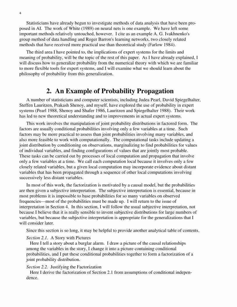
Section 2.1. A Story with PicturesHere I tell a story about a burglar alarm. I draw a picture of the causal relationships

among the variables in the story, I change it into a picture containing conditionalprobabilities, and I put these conditional probabilities together to form a factorization of ajoint probability distribution.

Section 2.2. Justifying the FactorizationHere I derive the factorization of Section 2.1 from assumptions of conditional indepen-

dence.

5

Section 2.3. Probabilities for Individual VariablesWe saw in the first section that factorization allows us to construct many probabilities

from a few probabilities. Here I show that it also allows the efficient computation ofprobabilities for individual variables. These benefits can be obtained from anyfactorization involving the same clusters of variables. The individual factors need not beprobabilities.

Section 2.4. Posterior ProbabilitiesI want posterior probabilities about the burglar alarm—probability judgments that take

all my information into account. The factorization we studied in the preceding sections isa factorization of the prior, not of the posterior. By adding an indicator function for eachobserved variable, we get a factorization of the posterior. This enables us to computeposterior probabilities for individual variables.

Section 2.5. Join TreesLocal computation works for the story of the burglar alarm because the clusters of vari-

ables involved in the factorization can be arranged in a join tree. In general, this will nothappen. To get a join tree, we must enlarge the clusters.

My purpose in this section is to make the simplicity of the ideas as clear as possible. I have nottried to be comprehensive. For a more thorough treatment, see Shafer and Shenoy (1988, 1990).

Figure 1.

The causal structure

of the story of the burglar

alarm.

E B

ER EO EA

A

PT AL

PC GW GH WH

GP GC WC

Earthquake Burglary

Earthquake reported onradio.

Earthquake felt atoffice.

Earthquake triggersalarm.

Alarm goes off.

Alarm loud enough forneighbors to hear.

Police try to call.

I get policecall.

Gibbons is wacky.

Gibbons hears thealarm.

Watson hears the alarm.

Gibbons played pranks in past week.

Call about alarm from Gibbons

Confused callfrom Watson

6

2.1. A Story with PicturesIn this section, I tell a story about a burglar alarm, a story first told, in a simpler form, by

Judea Pearl (1988, pp. 42-52). I draw a picture that displays the causal structure of this story andthen another picture that displays the conditional probabilities of the effects given their causes. Iinterpret this latter picture in terms of a factorization of my joint probability distribution for thevariables in the story.

Unlike the similar pictures drawn in path analysis (see, e.g., Duncan 1975), the pictures Idraw here are not substantive hypotheses, to be tested by statistical data. Rather, they are guidesto subjective judgement in a situation where there is little data relative to the number of variablesbeing considered. We are using a presumed causal structure to guide the construction ofsubjective probabilities. The conditional probabilities are building blocks in that construction.

The Story. My neighbor Mr. Gibbons calls me at my office at UCLA to tell me he has heardmy burglar alarm go off. (No, I don't work at UCLA, but it is easiest to tell the story in the firstperson.) His call leaves me uncertain about whether my home has been burglarized. The alarmmight have been set off instead by an earthquake. Or perhaps the alarm did not go off at all.Perhaps the call is simply one of Gibbons's practical jokes. Another neighbor, Mr. Watson, alsocalls, but I cannot understand him at all. I think he is drunk. What other evidence do I haveabout whether there was an earthquake or a burglary? No one at my office noticed anearthquake, and when I switch the radio on for a few minutes, I do not hear any reports aboutearthquakes in the area. Moreover, I should have heard from the police if the burglar alarm wentoff. The police station is notified electronically when the alarm is triggered, and if the policewere not too busy they would have called my office.

Perhaps you found Figure 1 useful as you organized this story in your mind. It gives a roughpicture of the story's causal structure. A burglary can cause the alarm to go off, hearing thealarm go off can cause Mr. Gibbons to call, etc.

7

Figure 2.

The causal structure

and the observations.

E B

ER EO EA

A

PT AL

PC GW GH WH

GP GC WC

Earthquake Burglary




Alarm goes off.


Police try to call.

I get policecall.

Gibbons is wacky.






nnoo nnoo

nnoo

nnoo yyeess yyeess

8

Figure 3.

The factorization

of my prior distribution.

E B

ER EO EA

A

PT AL

PC GH WH

GP GC WC

P( er,eo,ea | e )

P(a | ea,b)

P(gp | gw)

P(e) P(b)

P(al | a)

P(pc | pt) P(gh | al) P(wh | al)

P(gc | gw,gh) P(wc | wh)

P(pt | a)

GWP(gw)

ER,EO,EA,E

A,EA,B

PT,A AL,A

PC,PT GH,AL WH,AL

GC,GW,GH WC,WHGP,GW

Figure 1 shows only this causal structure. Figure 2 shows more; it also shows what I actuallyobserved. Gibbons did not play any other pranks on me during the preceding week (GP=no).Gibbons and Watson called (GC=yes, WC=yes), but the police did not (PC=no). I did not feel anearthquake at the office (EO=no), and I did not hear any report about an earthquake on the radio(ER=no).

I will construct one subjective probability distribution based on the evidence represented byFigure 1, and another based on the evidence represented by Figure 2. Following the usual termi-nology of Bayesian probability theory, I will call the first my prior distribution, and second myposterior distribution. The posterior distribution is of greatest interest; it gives probabilitiesbased on all my evidence. But we will study the prior distribution first, because it is much easierto work with. Only in Section 2.4 will we turn to the posterior distribution.

A Probability Picture. It is possible to interpret Figure 1 as a set of conditions on mysubjective probabilities, but the interpretation is complicated. So I want to call your attention toa slightly different picture, Figure 3, which conveys probabilistic information very directly.

I have constructed Figure 3 from Figure 1 by interpolating a box between each child and itsparents. In the box, I have put conditional probabilities for the child given the parents. In onecase (the case of E and its children, ER, EO, and EA), I have used a single box for severalchildren. In other cases (such as the case of A and its children, PT and AL), I have used separateboxes for each child. I have also put unconditional probabilities in the circles that have noparents.

9

The meaning of Figure 3 is simple: I construct my prior probability distribution for thefifteen variables in Figure 1 by multiplying together the functions (probabilities and conditionalprobabilities) in the boxes and circles:

P(e,er,eo,ea,b,a,pt,pc,al,gh,wh,gw,gp,gc,wc) = P(e) . P(er,eo,ea|e) . P(b) . P(a|ea,b) . P(pt|a) . P(pc|pt) . P(al|a) .P(gh|al) . P(wh|al) . P(gw) . P(gp|gw) . P(gc|gw,gh) . P(wc|wh). (1)

I may not actually perform the multiplication numerically. But it defines my prior probabilitydistribution in principle, and as we shall see, it can be exploited to find my prior probabilities forindividual variables.

I will call (1) a factorization of my prior probability distribution. This name can bemisleading, for it suggests that the left-hand side was specified in some direct way and thenfactored. The opposite is true; we start with the factors and multiply them together,conceptually, to define the distribution. Once this is clearly understood, however, “factorization”is a useful word.

Why should I define my prior probability distribution in this way? Why should I want or ex-pect my prior probabilities to satisfy (1)? What use is the factorization? The best way to startanswering these questions is to make the example numerical, by listing possible values of thevariables and their numerical probabilities. This by itself will make the practical significance ofthe factorization clearer, and it will give us a better footing for further abstract discussion.

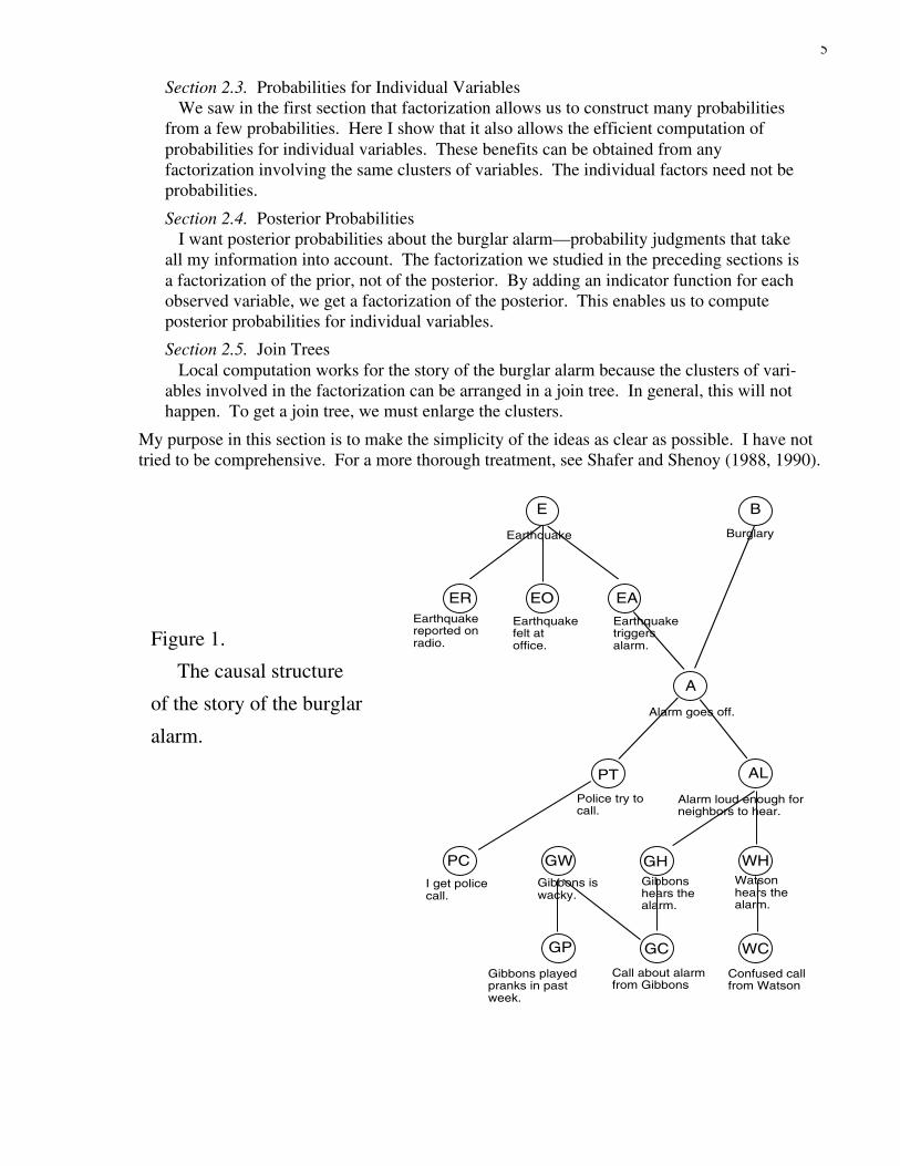
Frames. There are fifteen variables in my story—E, ER, EO, B, and so on. The lower caseletters in Figure 3—e, er,eo, b, and so on—represent possible values of these variables. What arethese possible values?

For simplicity, I have restricted most of the variables to two possible values—yes or no. Butin order to make the generality of the ideas clear, I have allowed two of the variables, PT andGW, to have three possible values. The police can try to call not at all, some, or a lot. Mr.Gibbons's level of wackiness this week can be low, medium, or high. This gives the sets ofpossible values shown in Figure 4. We can call these sets samples spaces or frames for thevariables.

10

Figure 4.

The frames.

E B

ER EO EA

A

PT AL

PC GW GH WH

GP GC WC

Earthquake Burglary




Alarm goes off.


Police try to call.

I get policecall.

Gibbons is wacky.




yesno

yesno

yesno

yesno

yesno

yesno

yesno

yesno

yesno

yesno

yesno

yesno

lowmediumhigh

not at allsomea lot

yesno



Probability Notation. The expressions in Figure 3 follow the usual notational conventionsof probability theory:

P(e) stands for “my prior probability that E=e,”P(a|ea,b) stands for “my prior probability that A=a, given that EA=ea and B=b,”P(er,eo,ea|e) stands for “my prior probability that ER=er and EO=eo and EA=ea, given that

E=e,”and so on.

Each of these expression stands not for a single number but rather for a whole set of num-bers—one number for each choice of values for the variables. In other words, the expressionsstand for functions. This probability notation differs, however, from the standard mathematicalnotation for functions. In mathematical notation, f(x) and g(x) are generally different functions,while f(x) and f(y) are the same function. Here, however, P(e) and P(b) are different functions.The first gives my probabilities for E, while the second gives my probabilities for B.

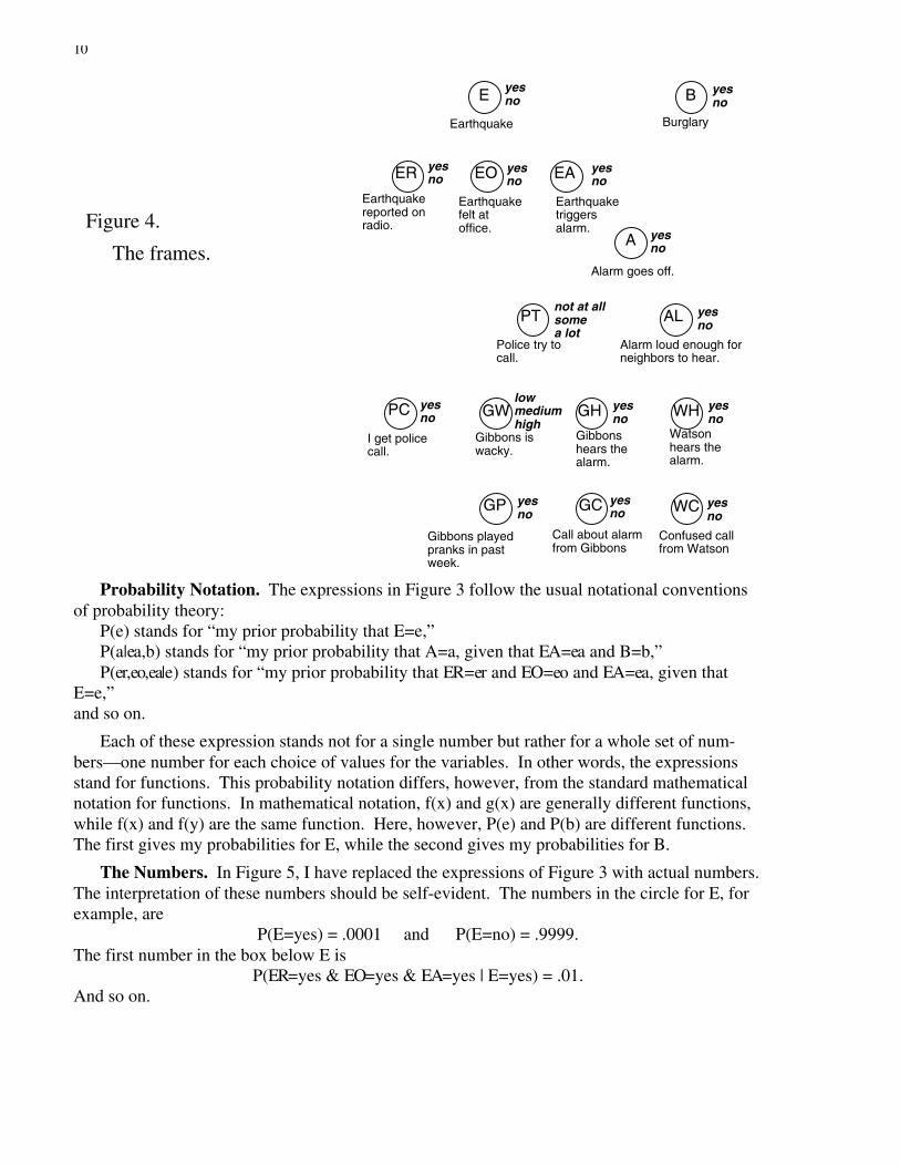
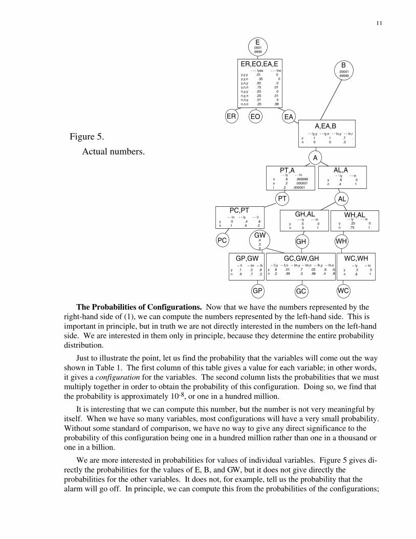
The Numbers. In Figure 5, I have replaced the expressions of Figure 3 with actual numbers.The interpretation of these numbers should be self-evident. The numbers in the circle for E, forexample, are

P(E=yes) = .0001 and P(E=no) = .9999.The first number in the box below E is

P(ER=yes & EO=yes & EA=yes | E=yes) = .01.And so on.

11

Figure 5.

Actual numbers.

E

B

ER EO EA

A

PT AL

PC GH WH

GP GC WC

P(er,eo,ea|e)

P(a|ea,b)

P(al|a)

P(pc|pt) P(gh|al) P(wh|al)

P(pt|a)

GW

- - - |yes - - - |noy,y,y .01 0y,y,n .35 0y,n,y .05 0y,n,n .15 .01n,y,y .03 0n,y,n .20 .01n,n,y .01 0n,n,n .20 .98

- - |y,y - - |y,n - - |n,y - - |n,ny 1 1 .7 .n 0 0 .3 .

- - |y - - |n y .6 0 n .4 1

- - |n - - |s - - |l y 0 .4 .8n 1 .6 .2

- - |y - - |n y .5 0 n .5 1

.0001

.9999

.00001

.99999

-- |y -- |n y .2 0 n .8 1

-- |l,y -- |l,n -- |m,y -- |m,n -- |h,y -- |h,ny .8 .01 .7 .02 .6 .04n .2 .99 .3 .98 .4 .96

-- |l -- |m -- |hy .1 .3 .8n .9 .7 .2

.4

.3

.3

- - |y - - |n n .6 .999998 s .2 .000001l .2 .000001

- - |y - - |n y .25 0 n .75 1

ER,EO,EA,E

A,EA,B

PT,A AL,A

PC,PT GH,AL WH,AL

GC,GW,GH WC,WHGP,GW

The Probabilities of Configurations. Now that we have the numbers represented by theright-hand side of (1), we can compute the numbers represented by the left-hand side. This isimportant in principle, but in truth we are not directly interested in the numbers on the left-handside. We are interested in them only in principle, because they determine the entire probabilitydistribution.

Just to illustrate the point, let us find the probability that the variables will come out the wayshown in Table 1. The first column of this table gives a value for each variable; in other words,it gives a configuration for the variables. The second column lists the probabilities that we mustmultiply together in order to obtain the probability of this configuration. Doing so, we find thatthe probability is approximately 10-8, or one in a hundred million.

It is interesting that we can compute this number, but the number is not very meaningful byitself. When we have so many variables, most configurations will have a very small probability.Without some standard of comparison, we have no way to give any direct significance to theprobability of this configuration being one in a hundred million rather than one in a thousand orone in a billion.

We are more interested in probabilities for values of individual variables. Figure 5 gives di-rectly the probabilities for the values of E, B, and GW, but it does not give directly theprobabilities for the other variables. It does not, for example, tell us the probability that thealarm will go off. In principle, we can compute this from the probabilities of the configurations;

12

we find the probabilities of all the configurations in which A=yes, and we add these probabilitiesup. As we will see in Section 2.3, however, there are much easier ways to find the probabilitythat A=yes.

For the sake of readers who are not familiar with probability theory, let me explain at thispoint two terms that I will use in this context: joint and marginal. A probability distribution fortwo or more variables is called a joint distribution. Thus the probability for a configuration is ajoint probability. If we are working with a joint probability distribution for a certain set ofvariables, then the probability distribution for any subset of these variables, or for any individualvariable, is called a marginal distribution. Thus the probability for an individual variable takinga particular value is a marginal probability. Computing such probabilities is the topic of Section2.3.

Table 1.

Computing the

probability of a

configuration.

E=yes P(E=yes) 0.0001ER=yesEO=no P(ER=yes&EO=no&EA=yes|E=yes) 0.05EA=yesB=no P(B=no) 0.99999A=yes P(A=yes|EA=yes&B=no) 1.0PT=a lot P(PT=a lot|A=yes) 0.2PC=no P(PC=no|PT=a lot) 0.2AL=yes P(AL=yes|A=yes) 0.6GH=yes P(GH=yes|AL=yes) 0.5WH=no P(WH=no|AL=yes) 0.75GW=low P(GW=low) 0.4GP=no P(GP=no|GW=low) 0.9GC=yes P(GC=yes|GW=low&GH=yes) 0.8WC=no P(WC=no|WH=no). 1.0

Many Numbers from a Few. How many configurations of our fifteen variables are there?Since thirteen of the variables have two possible values and two of them have three possible val-ues, there are

213 x 32 = 73,728configurations altogether.

One way to define my joint distribution for the fifteen variables would be to specify directlythese 73,728 numbers, making sure that they add to one. Notice how much more practical andefficient it is to define it instead by means of the factorization (1) and the 77 numbers in Figure5. I could not directly make up sensible numerical probabilities for the 73,728 configurations.Nor, for that matter, could I directly observe that many objective frequencies. But it may bepractical to make up or observe the 77 probabilities on the right-hand side. It is also much morepractical to store 77 rather than 73,728 numbers.

We could make do with even fewer than 77 numbers. Since each column of numbers in theFigure 5 adds to one, we can leave out the last number in each column without any loss of infor-mation, and this will reduce the number of numbers we need to specify and store from 77 to 46.This reduction is unimportant, though, compared with the reduction from 73,728 to 77.Moreover, it is relatively illusory. When we specify the numbers, we do want to think about the

13

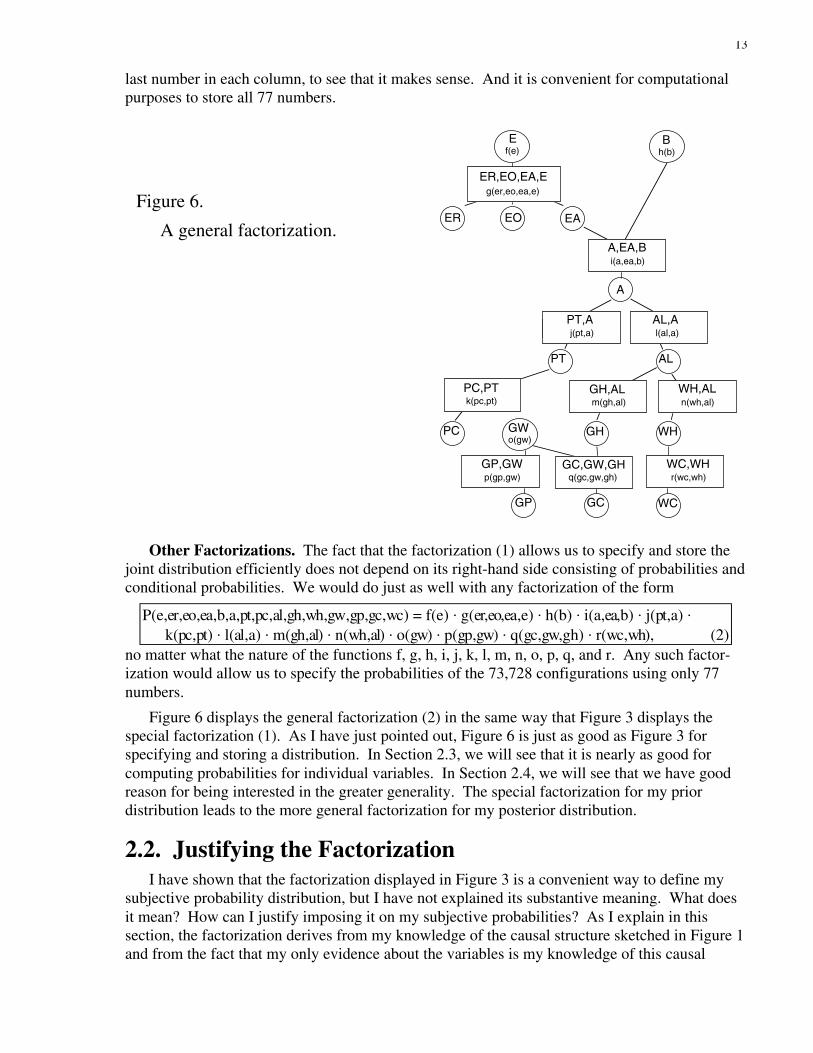
last number in each column, to see that it makes sense. And it is convenient for computationalpurposes to store all 77 numbers.

Figure 6.

A general factorization.

E B

ER EO EA

PT AL

PC GH WH

GP GC WC

P(a|ea,b)

P(gp|gw)

f(e) h(b)

P(al|a)


P(gc|gw,gh) P(wc|wh)

P(pt|a)

GWP(gw)

g(er,eo,ea,e)

ER,EO,EA,E

i(a,ea,b)A,EA,B

A

j(pt,a)PT,A

l(al,a)AL,A

GWo(gw)

k(pc,pt)PC,PT

m(gh,al)GH,AL

n(wh,al)WH,AL

p(gp,gw)GP,GW

q(gc,gw,gh)GC,GW,GH

r(wc,wh)WC,WH

Other Factorizations. The fact that the factorization (1) allows us to specify and store thejoint distribution efficiently does not depend on its right-hand side consisting of probabilities andconditional probabilities. We would do just as well with any factorization of the form

P(e,er,eo,ea,b,a,pt,pc,al,gh,wh,gw,gp,gc,wc) = f(e) . g(er,eo,ea,e) . h(b) . i(a,ea,b) . j(pt,a) . k(pc,pt) . l(al,a) . m(gh,al) . n(wh,al) . o(gw) . p(gp,gw) . q(gc,gw,gh) . r(wc,wh), (2)

no matter what the nature of the functions f, g, h, i, j, k, l, m, n, o, p, q, and r. Any such factor-ization would allow us to specify the probabilities of the 73,728 configurations using only 77numbers.

Figure 6 displays the general factorization (2) in the same way that Figure 3 displays thespecial factorization (1). As I have just pointed out, Figure 6 is just as good as Figure 3 forspecifying and storing a distribution. In Section 2.3, we will see that it is nearly as good forcomputing probabilities for individual variables. In Section 2.4, we will see that we have goodreason for being interested in the greater generality. The special factorization for my priordistribution leads to the more general factorization for my posterior distribution.

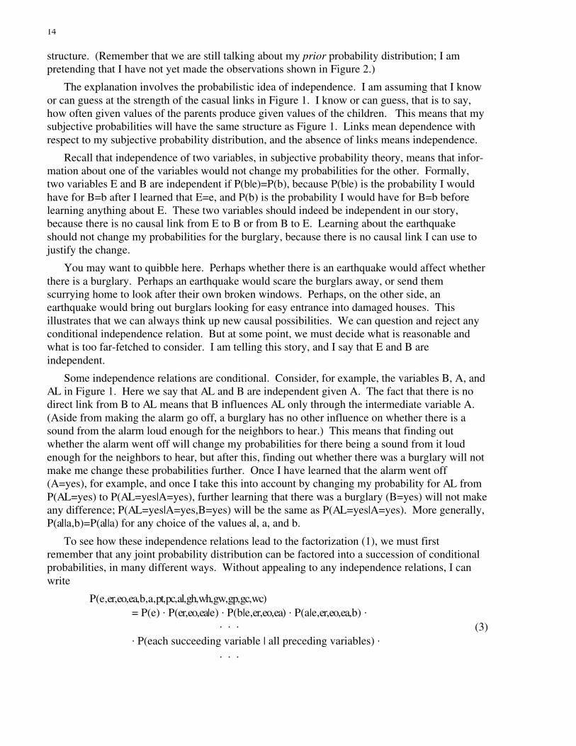
2.2. Justifying the FactorizationI have shown that the factorization displayed in Figure 3 is a convenient way to define my

subjective probability distribution, but I have not explained its substantive meaning. What doesit mean? How can I justify imposing it on my subjective probabilities? As I explain in thissection, the factorization derives from my knowledge of the causal structure sketched in Figure 1and from the fact that my only evidence about the variables is my knowledge of this causal

14

structure. (Remember that we are still talking about my prior probability distribution; I ampretending that I have not yet made the observations shown in Figure 2.)

The explanation involves the probabilistic idea of independence. I am assuming that I knowor can guess at the strength of the casual links in Figure 1. I know or can guess, that is to say,how often given values of the parents produce given values of the children. This means that mysubjective probabilities will have the same structure as Figure 1. Links mean dependence withrespect to my subjective probability distribution, and the absence of links means independence.

Recall that independence of two variables, in subjective probability theory, means that infor-mation about one of the variables would not change my probabilities for the other. Formally,two variables E and B are independent if P(b|e)=P(b), because P(b|e) is the probability I wouldhave for B=b after I learned that E=e, and P(b) is the probability I would have for B=b beforelearning anything about E. These two variables should indeed be independent in our story,because there is no causal link from E to B or from B to E. Learning about the earthquakeshould not change my probabilities for the burglary, because there is no causal link I can use tojustify the change.

You may want to quibble here. Perhaps whether there is an earthquake would affect whetherthere is a burglary. Perhaps an earthquake would scare the burglars away, or send themscurrying home to look after their own broken windows. Perhaps, on the other side, anearthquake would bring out burglars looking for easy entrance into damaged houses. Thisillustrates that we can always think up new causal possibilities. We can question and reject anyconditional independence relation. But at some point, we must decide what is reasonable andwhat is too far-fetched to consider. I am telling this story, and I say that E and B areindependent.

Some independence relations are conditional. Consider, for example, the variables B, A, andAL in Figure 1. Here we say that AL and B are independent given A. The fact that there is nodirect link from B to AL means that B influences AL only through the intermediate variable A.(Aside from making the alarm go off, a burglary has no other influence on whether there is asound from the alarm loud enough for the neighbors to hear.) This means that finding outwhether the alarm went off will change my probabilities for there being a sound from it loudenough for the neighbors to hear, but after this, finding out whether there was a burglary will notmake me change these probabilities further. Once I have learned that the alarm went off(A=yes), for example, and once I take this into account by changing my probability for AL fromP(AL=yes) to P(AL=yes|A=yes), further learning that there was a burglary (B=yes) will not makeany difference; P(AL=yes|A=yes,B=yes) will be the same as P(AL=yes|A=yes). More generally,P(al|a,b)=P(al|a) for any choice of the values al, a, and b.

To see how these independence relations lead to the factorization (1), we must firstremember that any joint probability distribution can be factored into a succession of conditionalprobabilities, in many different ways. Without appealing to any independence relations, I canwrite

P(e,er,eo,ea,b,a,pt,pc,al,gh,wh,gw,gp,gc,wc)= P(e) . P(er,eo,ea|e) . P(b|e,er,eo,ea) . P(a|e,er,eo,ea,b) .

. . . (3). P(each succeeding variable | all preceding variables) .

. . .

15

Here we have the probability for e, followed by the conditional probability for each succeedingvariable given all the preceding ones, except that I have grouped er, eo, and ea together. There arethirteen factors altogether.

Going from (3) to (1) is a matter of simplifying P(b|e,er,eo,ea) to P(b), P(a|e,er,eo,ea,b) toP(a|ea,b), and so on. Each of these simplifications corresponds to an independence relation.

Consider the first factor, P(b|e,er,eo,ea). The variables E, ER, EO, and EA, which have to dowith a possible earthquake, have no influence on B, whether there was a burglary. So B is un-conditionally independent of E, ER, EO, and EA; knowing the values of E, ER, EO, and EA wouldnot affect my probabilities for B. In symbols: P(b|e,er,eo,ea) = P(b).

The next factor I need to simplify is P(a|e,er,eo,ea,b). Once I know whether or not anearthquake triggered the alarm (this is what the value of EA tells me) and whether there was aburglary, further earthquake information will not change further my probabilities about whetherthe alarm went off. So P(a|e,er,eo,ea,b) = P(a|ea,b); A is independent of E, ER, and EO given EAand B.

I will leave it to the reader to simplify the remaining factors. In each case, the simplificationis achieved by identifying my evidence with the causal structure and then making a judgment ofindependence based on the lack of direct causal links. In each case, the judgment is that thevariable whose probability is being considered is independent of the variables we leave out giventhe variables we leave in.

One point deserves further discussion. In Figure 3, I used one box for the three children of Ebut separate boxes for the children of A and separate boxes for the children of GW. This choice,which is reflected in children of E entering (1) together while the children of A and GW enterseparately, is based on my judgment that the children of E are dependent given E, while thechildren in the other cases are independent given their parents. This again is based on causalreasoning. In my version of the story, PT and AL are independent given A. The mechanism bywhich the alarm alerts the police is physically independent of the mechanism by which it makesnoise; hence if it goes off, whether it is loud enough for the neighbors to hear is independent ofwhether the police try to call. On the other hand, if there is an earthquake at my home, whetherit is strong enough to be felt at my office is not independent of whether it is important enough tobe reported on the radio or strong enough to trigger my burglar alarm.

Factorization or Independence? Since I have used independence relations to justify myfactorization, you might feel that I should have started with independence rather than with factor-ization. Isn't it more basic?

Most authors, including Pearl (1988) and Lauritzen and Spiegelhalter (1988) haveemphasized independence rather than factorization. These authors do not use pictures such asFigure 3. Instead, they emphasize directed acyclic graphs, pictures like Figure 1, which theyinterpret directly as sets of independence relations.

There are several reasons to emphasize factorization rather than independence. First, andmost importantly, it is factorization rather than independence that generalizes most fruitfullyfrom probability to other approaches to handling uncertainty in expert systems. This is mymessage in Sections 3 and 4 of this paper.

Second, even within the context of probability, an emphasis on independence obscures theessential simplicity of the local computations that we will study shortly. Local computation re-quires factorization, but it does not require all the independence relations implied by a directedacyclic graph. This is of practical importance when we undertake to compute posterior

16

probabilities, for in this case we start only with a factorization. An insistence on working with adirected acyclic graph for the posterior will lead to conceptual complication and computationalinefficiency.

Third, the theory of independence is a detour from the problems of most importance. Onlysome of the independence relations suggested by the absence of links in Figure 1 were needed tojustify the factorization. Do these imply the others? What other subsets of all the independencerelations suggested by the figure are sufficient to imply the others? These are interesting andsometimes difficult questions (see, e.g., Geiger 1990), but they have minimal relevance to com-putation and implementation.

2.3. Probabilities for Individual VariablesIn Section 2.1, I pointed out that the factorizations of Figures 3 and 6 allow me to specify and

store probabilities for many configurations using only a few numbers. In this section, we willstudy a second benefit of these factorizations. They allow me to compute the marginalprobabilities for individual variables efficiently, using only local computations.

I begin by demonstrating how to obtain marginals from Figure 3. The method is simple, andreaders practiced in probability calculations will see immediately why it works. Then I willexplain how to obtain marginals for the more general factorization of Figure 6. As we will see,there is slightly more work to do in this case, but the generality of the case makes the simplicityof the method clear. We do not need the more subtle properties of probabilistic conditionalindependence. We need only the distributivity of multiplication over addition and a property oftree used by Figures 3 and 6—it is a join tree.

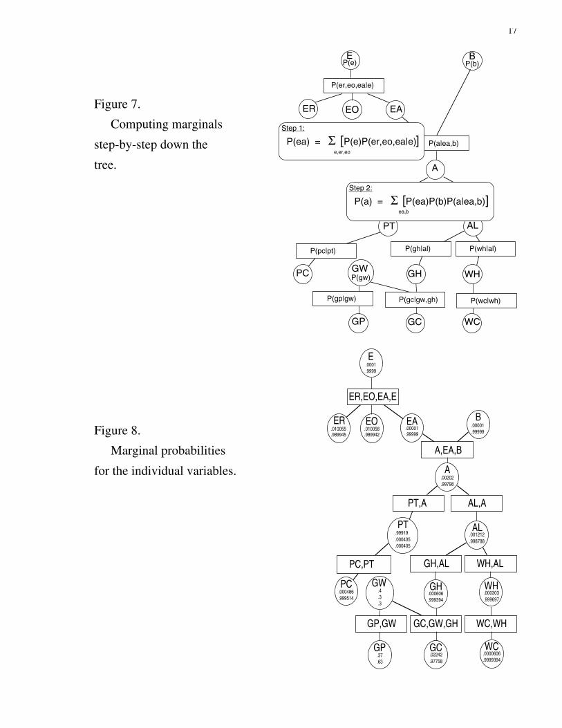
Marginals from the Special Factorization. Suppose we want my probabilities for A,whether the alarm went off. Figure 7 shows how to find them from the factorization of Figure 3.First we compute the marginal for EA. Then we use it to compute the marginal for A.

This is practical and efficient. It avoids working with all 73,728 configurations, which wewould have to do if we had defined the joint directly, without a factorization. In the first step, wehave two summations (one for EA=yes and one for EA=no), each involving only eight terms. Inthe second step, we again have two summations, each involving only four terms.

We can compute the marginal for any variable we want in this way. We simply keep goingdown the tree until we come to that variable. At each step, we compute the marginal for aparticular variable from factors that involve only it and its parents. These factors are either givenin the beginning or computed in the preceding steps.

17

Figure 7.

Computing marginals

step-by-step down the

tree.

E B

ER EO EA

A

PT AL

PC GH WH

GP GC WC

P(er,eo,ea|e)

P(a|ea,b)

P(gp|gw)

P(e) P(b)

P(al|a)



P(pt|a)

Step 1:

P(ea) = Σ [P(e)P(er,eo,ea|e)] e,er,eo

Step 2:

P(a) = Σ [P(ea)P(b)P(a|ea,b)] ea,b

GWP(gw)

Figure 8.

Marginal probabilities

for the individual variables.

E.0001.9999

GW.4.3.3

A

PC,PT GH,AL WH,AL

GP,GW GC,GW,GH WC,WH

PT,A AL,A

ER.010055.989945

EO.010058.989942

EA.00001.99999

B.00001.99999

.00202

.99798

PT.99919.000405.000405

AL.001212.998788

WH.000303.999697

GH.000606.999394

GC.02242.97758

GP.37.63

PC.000486.999514

ER,EO,EA,E

A,EA,B

WC.0000606.9999394

18

Figure 8 shows the numerical results, using the inputs of Figure 5. Each circle now containsthe marginal probabilities for its variable.

Why does this method work? Why are the formulas in Figure 7 correct? If you are practicedenough with probability, you may feel that the validity of the formulas and the method is tooobvious to require much explanation. Were you to try to spell out an explanation, however, youwould find it fairly complex.

I will spell out an explanation, but I will do it in a roundabout way, in order to make clear thegenerality of the method. I will begin by redescribing the method in a leisurely way. This willhelp us sort out what depends on the particular properties of the special factorization in Figure 3from what will work for the general factorization in Figure 6.

The Leisurely Redescription. My redescription involves pruning branches as I go down thetree of Figure 3. For reasons that will become apparent only in Section 2.5, I prune very slowly.At each step, I prune only circles or only boxes.

On the first step, I prune only circles from Figure 3. I prune the circle E, the circle B, thecircle ER, and the circle EO. When I prune a circle that contains a function (E and B containfunctions, but ER and EO do not), I put that function in the neighboring box, where it multipliesthe function already there. This gives Figure 9.

On the next step, I prune the box ER,EO,EA,E from Figure 9. I sum the variables ER, EO,and E out of the function in the box, and I put the result, P(ea) in the neighboring circle. Thisgives Figure 10.

Next I prune the circle EA, putting the factor it contains into the neighboring box. This givesFigure 11.

Then I prune the box A,EA,B. I sum the variables EA and B out of the function in this box,and I put the result, P(a), in the neighboring circle. This gives Figure 12.

Here are the rules I am following:Rule 1. I only prune twigs. (A twig is a circle or box that has only one

neighbor; the circle EO is a twig in Figure 3, and the box A,EA,B is a twig inFigure 11.)

Rule 2. When I prune a circle, I put its contents, if any, in the neighboringbox, where it will be multiplied by whatever is already there.

Rule 3. When I prune a box, I sum out from the function it contains anyvariables that are not in the neighboring circle, and then I put the result in thatcircle.

In formulating Rules 2 and 3, I have used the fact that a twig in a tree has a unique neighbor. Itis useful to have a name for this unique neighbor; I call it the twig's branch.

I ask you to notice two properties of the process governed by these rules. First, in eachfigure, from Figure 9 to Figure 12, the functions in the boxes and the circles form a factorizationfor the joint probability distribution of the variables that remain in the picture. Second, thefunction I put into a circle is always the marginal probability distribution for the variable in thatcircle.

The second property is convenient, because it is the marginal probability distributions that wewant. But as we will see shortly, the first property is more general. It will hold when we prunethe general factorization of Figure 6, while the second property will not. Moreover, the firstproperty will hold when we prune twigs from below just as it holds when we prune twigs fromabove. This means that the first property is really all we need. If we can prune twigs while

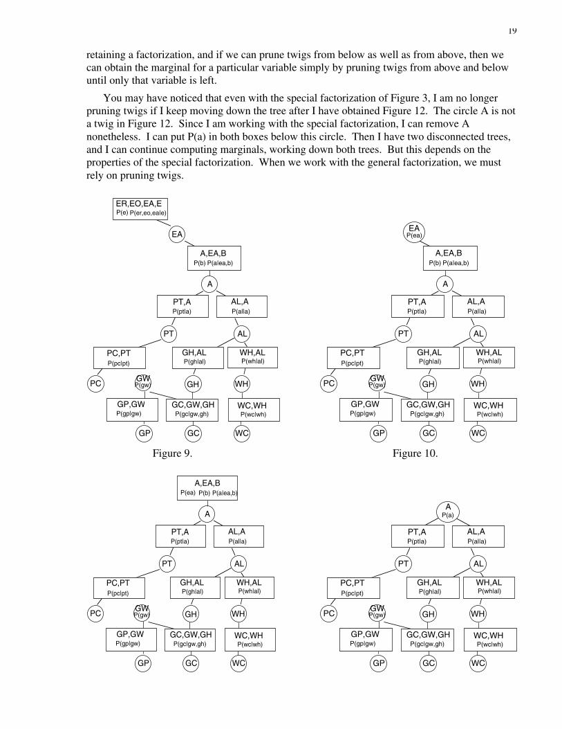
19

retaining a factorization, and if we can prune twigs from below as well as from above, then wecan obtain the marginal for a particular variable simply by pruning twigs from above and belowuntil only that variable is left.

You may have noticed that even with the special factorization of Figure 3, I am no longerpruning twigs if I keep moving down the tree after I have obtained Figure 12. The circle A is nota twig in Figure 12. Since I am working with the special factorization, I can remove Anonetheless. I can put P(a) in both boxes below this circle. Then I have two disconnected trees,and I can continue computing marginals, working down both trees. But this depends on theproperties of the special factorization. When we work with the general factorization, we mustrely on pruning twigs.

EA

A

PT AL

PC GH WH

GP GC WC

P(al|a)P(pt|a)

GWP(gw)

P(a|ea,b)A,EA,B

P(pc|pt) P(gh|al) P(wh|al)PC,PT GH,AL WH,AL

P(wc|wh)P(gc|gw,gh)P(gp|gw)GP,GW GC,GW,GH WC,WH

P(er,eo,ea|e)ER,EO,EA,E

PT,A AL,A

P(b)

P(e)

EA

A

PT AL

PC GH WH

GP GC WC

P(al|a)P(pt|a)

GWP(gw)

P(a|ea,b)A,EA,B



PT,A AL,A

P(b)

P(ea)

Figure 9. Figure 10.

A

PT AL

PC GH WH

GP GC WC

P(al|a)P(pt|a)

GWP(gw)

P(a|ea,b)A,EA,B



PT,A AL,A

P(b)P(ea)

A

PT AL

PC GH WH

GP GC WC

P(al|a)P(pt|a)

GWP(gw)

P(a)



PT,A AL,A

20


Marginals from the General Factorization. Now I prune the general factorization ofFigure 6. Figures 13 to 16 show what happens as I prune the circles and boxes above A.

Notice that I must invent some names for the functions I get when I sum out the variables.Going from Figure 13 to Figure 14 involves summing ER, EO, and E out of f(e).g(er,eo,ea,e); Iarbitrarily call the result g*(ea). In symbols:

g*(ea) = ∑e,er,eo

[f(e).g(er,eo,ea,e)] .

Similarly, i*(a) is the result of summing EA and B out of g*(ea).h(b).i(a,ea,b):

i*(a) = ∑ea,b

[g*(ea).h(b).i(a,ea,b)] .

I want to convince you that Figures 13 to 16 have the same property as Figure 6. In eachcase, the functions in the picture constitute a factorization of the joint probability distribution forthe variables in the picture.

EA

PT AL

PC GH WH

GP GC WC

P(a|ea,b)

P(gp|gw)

f(e)

P(al|a)



P(pt|a)

GWP(gw)

g(er,eo,ea,e)

ER,EO,EA,E

i(a,ea,b)

A,EA,B

A

j(pt,a)PT,A

l(al,a)AL,A

GWo(gw)

k(pc,pt)PC,PT

m(gh,al)GH,AL

n(wh,al)WH,AL

p(gp,gw)GP,GW

q(gc,gw,gh)GC,GW,GH

r(wc,wh)WC,WH

h(b)

EA

PT AL

PC GH WH

GP GC WC

P(a|ea,b)

P(gp|gw)

P(al|a)



P(pt|a)

GWP(gw)

g*(ea)

i(a,ea,b)

A,EA,B

A

j(pt,a)PT,A

l(al,a)AL,A

GWo(gw)

k(pc,pt)PC,PT

m(gh,al)GH,AL

n(wh,al)WH,AL

p(gp,gw)GP,GW

q(gc,gw,gh)GC,GW,GH

r(wc,wh)WC,WH

h(b)


Figure 13 obviously has this property, because it has the same functions as Figure 6. It is lessobvious that Figure 14 has the property. It is here that we must use the distributivity ofmultiplication.

In general, to obtain the joint distribution of a set of variables from the joint distribution of alarger set of variables, we must sum out the variables that we want to omit. So if we omit ER,EO, and E from the joint distribution of all fifteen variables, the joint distribution of the twelvethat remain is given by

21

P(ea,b,a,pt,pc,al,gh,wh,gw,gp,gc,wc)

= ∑e,er,eo

P(e,er,eo,ea,b,a,pt,pc,al,gh,wh,gw,gp,gc,wc) .

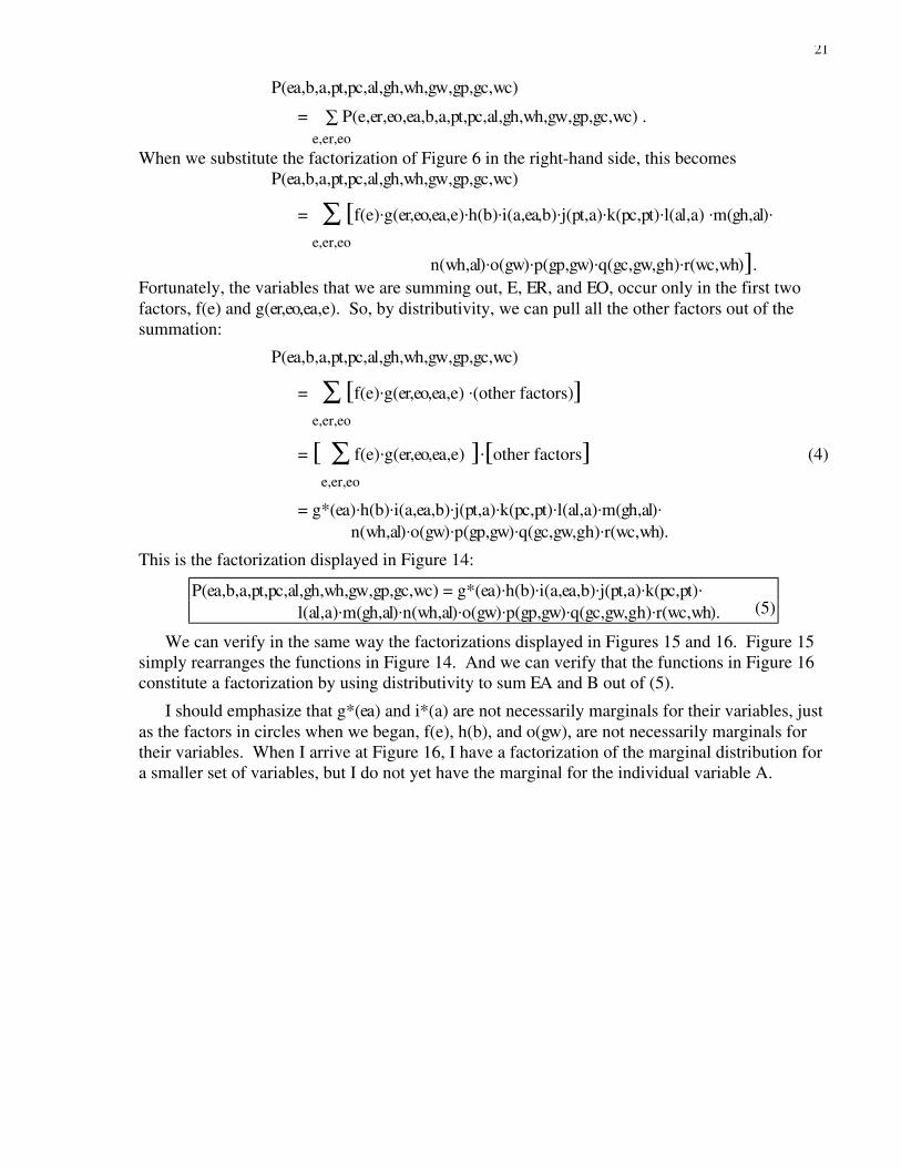
When we substitute the factorization of Figure 6 in the right-hand side, this becomesP(ea,b,a,pt,pc,al,gh,wh,gw,gp,gc,wc)

= ∑e,er,eo

[f(e).g(er,eo,ea,e).h(b).i(a,ea,b).j(pt,a).k(pc,pt).l(al,a) .m(gh,al).

n(wh,al).o(gw).p(gp,gw).q(gc,gw,gh).r(wc,wh)].Fortunately, the variables that we are summing out, E, ER, and EO, occur only in the first twofactors, f(e) and g(er,eo,ea,e). So, by distributivity, we can pull all the other factors out of thesummation:

P(ea,b,a,pt,pc,al,gh,wh,gw,gp,gc,wc)

= ∑e,er,eo

[f(e).g(er,eo,ea,e) .(other factors)]

= [ ∑e,er,eo

f(e).g(er,eo,ea,e) ].[other factors] (4)

= g*(ea).h(b).i(a,ea,b).j(pt,a).k(pc,pt).l(al,a).m(gh,al).

n(wh,al).o(gw).p(gp,gw).q(gc,gw,gh).r(wc,wh).

This is the factorization displayed in Figure 14:

P(ea,b,a,pt,pc,al,gh,wh,gw,gp,gc,wc) = g*(ea).h(b).i(a,ea,b).j(pt,a).k(pc,pt).

l(al,a).m(gh,al).n(wh,al).o(gw).p(gp,gw).q(gc,gw,gh).r(wc,wh). (5)

We can verify in the same way the factorizations displayed in Figures 15 and 16. Figure 15simply rearranges the functions in Figure 14. And we can verify that the functions in Figure 16constitute a factorization by using distributivity to sum EA and B out of (5).

I should emphasize that g*(ea) and i*(a) are not necessarily marginals for their variables, justas the factors in circles when we began, f(e), h(b), and o(gw), are not necessarily marginals fortheir variables. When I arrive at Figure 16, I have a factorization of the marginal distribution fora smaller set of variables, but I do not yet have the marginal for the individual variable A.

22

PT AL

PC GH WH

GP GC WC

P(a|ea,b)

P(gp|gw)

P(al|a)



P(pt|a)

GWP(gw)

i(a,ea,b)

A,EA,B

A

j(pt,a)PT,A

l(al,a)AL,A

GWo(gw)

k(pc,pt)PC,PT

m(gh,al)GH,AL

n(wh,al)WH,AL

p(gp,gw)GP,GW

q(gc,gw,gh)GC,GW,GH

r(wc,wh)WC,WH

h(b)g*(ea)

PT AL

PC GH WH

GP GC WC

P(gp|gw)

P(al|a)



P(pt|a)

GWP(gw)

A

j(pt,a)PT,A

l(al,a)AL,A

GWo(gw)

k(pc,pt)PC,PT

m(gh,al)GH,AL

n(wh,al)WH,AL

p(gp,gw)GP,GW

q(gc,gw,gh)GC,GW,GH

r(wc,wh)WC,WH

i*(a)


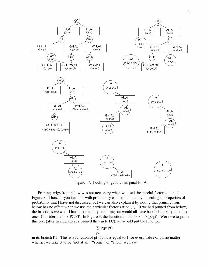
To obtain the marginal for A, I must peel from below in Figure 16. This process is laid out ineight steps in Figure 17. In the first step, I prune four circles, PC, GP, GC, and WC, none ofwhich contains a function. In the second step, I prune the box PC,PT, the box GP,GW, and thebox WC,WH. Each time, I sum out a variable and put the result into the box's branch, k*(pt) intoPT, p*(gw) into GW, and r*(wh) into WH. And so on. At each step, the functions in the pictureform a factorization for the distribution for the variables remaining. At the end, only the variableA and the function j*(a).i*(a).l*(a) remain. A “factorization” of a distribution consisting of asingle function is simply the distribution itself. So j*(a).i*(a).l*(a) is the marginal P(a).

We can find the marginal for any other variable in the same way. We simply prune twigsuntil only that variable remains.

23

PT AL

GH WH

P(gp|gw)

P(al|a)



P(pt|a)

GWP(gw)

A

j(pt,a)PT,A

l(al,a)AL,A

GWo(gw)

k(pc,pt)PC,PT

m(gh,al)GH,AL

n(wh,al)WH,AL

p(gp,gw)GP,GW

q(gc,gw,gh)GC,GW,GH

r(wc,wh)WC,WH

i*(a)

PT AL

GH WH

P(al|a)

P(gh|al) P(wh|al)

P(gc|gw,gh)

P(pt|a)

GWo(gw)

A

j(pt,a)PT,A

l(al,a)AL,A

k*(pt)

m(gh,al)GH,AL

n(wh,al)WH,AL

p*(gw)

q(gc,gw,gh)GC,GW,GH

r*(wh)

i*(a)

AL

GH

P(al|a)

P(gh|al) P(wh|al)

P(gc|gw,gh)

P(pt|a)

A

j(pt,a)PT,A

l(al,a)AL,A

k*(pt)

m(gh,al)GH,AL

n(wh,al)WH,AL

q(gc,gw,gh)

GC,GW,GH

r*(wh)

i*(a)

o(gw)p*(gw)

AL

GH

P(al|a)

P(gh|al)

Aj*(a)

l(al,a)AL,A

m(gh,al)GH,AL

n*(al)

i*(a)

q*(gh)

AL

P(al|a)

P(gh|al)

Aj*(a)

l(al,a)AL,A

m(gh,al)GH,AL

n*(al)

i*(a)

q*(gh)

AL

P(al|a)

Aj*(a)

l(al,a)AL,A

m*(al) n*(al)

i*(a)

P(al|a)

Aj*(a)

l(al,a)AL,A

m*(al) n*(al)

i*(a)

A

j*(a) i*(a) l*(a)

Figure 17. Peeling to get the marginal for A.

Pruning twigs from below was not necessary when we used the special factorization ofFigure 3. Those of you familiar with probability can explain this by appealing to properties ofprobability that I have not discussed, but we can also explain it by noting that pruning frombelow has no affect when we use the particular factorization (1). If we had pruned from below,the functions we would have obtained by summing out would all have been identically equal toone. Consider the box PC,PT. In Figure 3, the function in this box is P(pc|pt). Were we to prunethis box (after having already pruned the circle PC), we would put the function

∑pc

P(pc|pt)

in its branch PT. This is a function of pt, but it is equal to 1 for every value of pt; no matterwhether we take pt to be “not at all,” “some,” or “a lot,” we have

24

∑pc

P(pc|pt) = P(PC=yes|pt) + P(PC=no|pt) = 1.

We can pass this function on to the box PT, and then on to the box PT,A, but it will make no dif-ference, because multiplying the function already in that box by one will not change it. Thishappens throughout the tree; the messages passed upwards will be identically equal to one andhence will not make any difference.

Join Trees. The tree in Figure 6 has one property that is essential in order for us to retain afactorization as we prune. When I pruned the twig ER,EO,EA,E, I summed out all the variablesthat were not in the branch, EA. My justification for doing this locally, equation (4), relied onthe fact that the variables I was summing out did not occur in any of the other factors. In otherwords, if a variable is not in the branch, it is not anywhere else in the tree either!

Each time I prune a box and sum out variables, I rely on this same condition. Each time, Iam able to sum locally because the only variable the box has in common with the rest of the treeis in its branch.

We can make a more general statement. If we think of Figure 6 as a tree in which all thenodes are sets of variables (ignoring the distinction between boxes and circles), then each timewe prune a twig, any variables that the twig has in common with the rest of the tree are in itsbranch. This is true when we prune boxes, for the box always has only one variable in commonwith the rest of the tree, and it is in the circle that serves as the box's branch. It is also true whenwe prune circles, for the single variable in the circle is always in the box that serves as thecircle's branch.

A tree that has sets of variables as nodes and meets the italicized condition in the precedingparagraph is called a join tree. As we will see in Section 2.5, local computation can beunderstood most clearly in the abstract setting of join trees.

Comparing the Effort. Possibly you are not yet convinced that the amount of computingneeded to find marginals for the general factorization of Figure 6 is comparable to the amountneeded for the special factorization of Figure 3. With the special factorization, we get marginalsfor all the variables by moving down the tree once, making local computations as we go. To geteven a single marginal from the general factorization, we must peel away everything else, fromabove and below, and getting a second marginal seems to require repeating the whole process.

In general, however, getting a second marginal does not require repeating the whole process,because if the two variables are close together in the tree, much of the pruning will be the same.Shafer and Shenoy (1988, 1990) explain how to organize the work so that all the marginals canbe computed with only about twice as much effort as it takes to compute any single marginal,even if the tree is very large. In general, computing all the marginals from the general factoriza-tion is only about twice as hard as moving down the tree once to compute all the marginals fromthe special factorization. This factor of two can be of some importance, but if the tree is large,the advantage of the special over the general factorization will be insignificant compared to theadvantage of both over the brute-force approach to marginalization that we would have to resortto if we did not have a factorization.

2.4. Posterior ProbabilitiesWe are now in a position to compute posterior probabilities for the story of the burglar alarm.

In this section, I will adapt the factorization of the prior distribution shown in Figure 3 to a

25

factorization of the posterior distribution, and then I will use the method of the preceding sectionto compute posterior probabilities for individual variables.

Notation for Posterior Probabilities. I have observed six of the fifteen variables:ER=no, EO=no, PC=no, GP=no, GC=yes, WC=yes.

I want to compute my posterior probabilities for the nine other variables based on these observa-tions. I want to compute, for example, the probabilities

P(B=yes | ER=no,EO=no,PC=no,GP=no,GC=yes,WC=yes) (6)and

P(B=no | ER=no,EO=no,PC=no,GP=no,GC=yes,WC=yes); (7)these are my posterior probabilities for whether there was a burglary. For the moment I willwrite er0 for the value “no” of the variable ER, I will write gc0 for the value “yes” of the variableGC, and so on. This allows me to write

P(b|er0,eo0,pc0,gp0,gc0,wc0)for my posterior probability distribution for B. This notation is less informative than (6) and (7),for it does not reveal which values of the variables I observed, but it is conveniently abstract.

In order to compute my posterior probabilities for individual variables, I need to work withmy joint posterior distribution for all fifteen variables, the distribution

P(e,er,eo,ea,b,a,pt,pc,al,gh,wh,gw,gp,gc,wc | er0,eo0,pc0,gp0,gc0,wc0). (8)As we will see shortly, I can write down a factorization for this distribution that fits into the sametree as our factorization of my prior distribution.

You may be surprised to hear that we need to work with my joint posterior distribution for allfifteen variables. It may seem wasteful to put all fifteen variables, including the six I have ob-served, on the left-hand side of the vertical bar in (8). Posterior to the observations, I have prob-ability one for specific values of these six variables. Why not leave them out, and work with thesmaller joint distribution for the nine remaining variables:

P(e,ea,b,a,pt,al,gh,wh,gw | er0,eo0,pc0,gp0,gc0,wc0)?We could do this, but it will be easier to explain what we are doing if we continue to work withall fifteen variables. We will waste some time multiplying and adding zeros—the probability in(8) will be zero if er is different from er0 or eo is different from eo0, etc. But this is a minormatter.

A Review of Conditional Probability. Since we are doing things a little differently thanusual, we need to go back to the basics.

In general, the probability of an event A given an event B is given by

P(A | B) = P(A & B)

P(B) (9)

So my posterior probability for the event B=b given the observation E=e0 is given by

P(B=b | E=e0) = P(B=b & E=e0)

P(E=e0) .

When we think of P(B=b | E=e0) as a distribution for B, with the observation e0 fixed, we usuallyabbreviate this to

P(b|e0) = K . P(B=b & E=e0),and we say that K is a constant. We often abbreviate it even further, to

P(b|e0) = K . P(b,e0).This last formula has a clear computational meaning. If we have a way of computing the jointdistribution P(b,e), then to get the conditional, we compute this joint with e0 substituted for e,and then we find K. Finding K is called renormalizing. Since the posterior probabilities for Bmust add to one, K will be the reciprocal of the sum of P(b,e0) over all b.

26

I want to include E on the left of the vertical bar in these formulas. So I use (9) again, toobtain

P(B=b & E=e | E=e0) = P(B=b & E=e & E=e0)

P(E=e0) .

I abbreviate this toP(b,e|e0) = K . P(B=b & E=e & E=e0). (10)

But what do I do next? I am tempted to write P(b,e,e0) for the probability on the right-hand side,but what is P(b,e,e0) in terms of the joint distribution for B and E? I need a better notation thanthis—one that makes the computational meaning clearer.

What I need is a notation for indicator functions.

Posterior Probabilities with Indicator Functions. Given a value e0 for a variable E, I willwrite Ee0 for the indicator function for E=e0. This is a function on the frame for E. It assignsthe number one to e0 itself, and it assigns the number zero to every other element of the frame.

In symbols:

Ee0(e) = 1 if e=e0

0 if e≠e0

In our story, the frame for E is {yes, no}. Thus the indicator function Eno, say, is given byEno(yes)=0 and Eno(no)=1.

Now let us look again at (10). It is easy to see that

P(B=b & E=e & E=e0) = P(b,e) if e=e0

0 if e≠e0 = P(b,e) .

1 if e=e0

0 if e≠e0 = P(b,e) . Ee0(e).

So we can write (10) using an indicator function:

P(b,e|e0) = K . P(b,e) . Ee0(e).

To condition a joint distribution on an observation, we simply multiply it by the indicatorfunction corresponding to the observation. We also need to find the constant K that will makethe posterior probabilities add up to one. It is the reciprocal of the sum of the P(b,e).Ee0(e) over

all b and e.

If we observe several variables, then the conditioning can be carried out step by step; we con-dition on the first observation, then condition the result on the second, etc. At each step, we sim-ply multiply by another indicator variable. We can leave the renormalization until the end.Briefly put, conditioning on several observations means multiplying by all the indicator variablesand then renormalizing.

The Burglar Alarm Again. I have six observations, so I multiply my prior by six indicatorfunctions:

P(e,er,eo,ea,b,a,pt,pc,al,gh,wh,gw,gp,gc,wc | er0,eo0,pc0,gp0,gc0,wc0)= K . P(e,er,eo,ea,b,a,pt,pc,al,gh,wh,gw,gp,gc,wc) . ERer0(er) .

EOeo0(eo) . PCpc0(pc) . GPgp0(gp) . GCgc0(gc) . WCwc0(wc).

At this point, we can simplify the notation. Instead of ERer0(er), I write ERno(er), and similarly

for the other observations. I also eliminate the subscripted expressions on the left-hand side.The posterior probability distribution is just another probability distribution. So I can give it asimple name—say Q. With these changes, we have

Q(e,er,eo,ea,b,a,pt,pc,al,gh,wh,gw,gp,gc,wc)

27

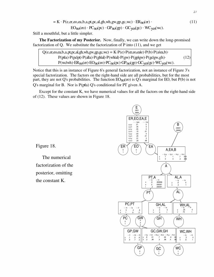
= K . P(e,er,eo,ea,b,a,pt,pc,al,gh,wh,gw,gp,gc,wc) . ERno(er) . (11)

EOno(eo) . PCno(pc) . GPno(gp) . GCyes(gc) . WCyes(wc).Still a mouthful, but a little simpler.

The Factorization of my Posterior. Now, finally, we can write down the long-promisedfactorization of Q. We substitute the factorization of P into (11), and we get

Q(e,er,eo,ea,b,a,pt,pc,al,gh,wh,gw,gp,gc,wc) = K.P(e).P(er,eo,ea|e).P(b).P(a|ea,b).

P(pt|a).P(pc|pt).P(al|a).P(gh|al).P(wh|al).P(gw).P(gp|gw).P(gc|gw,gh). (12)P(wc|wh).ERno(er).EOno(eo).PCno(pc).GPno(gp).GCyes(gc).WCyes(wc).

Notice that this is an instance of Figure 6's general factorization, not an instance of Figure 3'sspecial factorization. The factors on the right-hand side are all probabilities, but for the mostpart, they are not Q's probabilities. The function EOno(eo) is Q's marginal for EO, but P(b) is notQ's marginal for B. Nor is P(pt|a) Q's conditional for PT given A.

Except for the constant K, we have numerical values for all the factors on the right-hand sideof (12). These values are shown in Figure 18.

Figure 18.

The numerical

factorization of the

posterior, omitting

the constant K.

EAER01

EO01

E

A

GP GC WC

P(er,eo,ea|e)

P(a|ea,b)

P(al|a)

P(gh|al) P(wh|al)

P(pt|a)

- - - |yes - - - |noy,y,y .01 0y,y,n .35 0y,n,y .05 0y,n,n .15 .01n,y,y .03 0n,y,n .20 .01n,n,y .01 0n,n,n .20 .98

- - |y,y - - |y,n - - |n,y - - |n,ny 1 1 .7 .002n 0 0 .3 .998

- - |y - - |n y .6 0 n .4 1

- - |y - - |n y .5 0 n .5 1

.0001

.9999

-- |y -- |n y .2 0 n .8 1

-- |l,y -- |l,n -- |m,y -- |m,n -- |h,y -- |h,ny .8 .01 .7 .02 .6 .04n .2 .99 .3 .98 .4 .96

-- |l -- |m -- |hy .1 .3 .8n .9 .7 .2

- - |y - - |n n .6 .999998 s .2 .000001l .2 .000001

- - |y - - |n y .25 0 n .75 1

ER,EO,EA,E

A,EA,B

PT,A AL,A

GH,AL WH,AL

GC,GW,GH WC,WHGP,GW

GP GC WC01

10

10

GH WHPC01

GW.4.3.3

PT AL

B.00001.99999

PC,PT - - |n - - |s - - |l y 0 .4 .8n 1 .6 .2

28

We can now find Q's marginals for all the individual variables, using the method of thepreceding section. There is only one complication—the constant K. How do we find itefficiently? As it turns out, K will more or less fall out of the computation. If we leave K out ofthe right-hand side of (12), the final result will still need to be multiplied by K in order to sum toone. If, for example, we are finding the marginal for A, then the function j*(a).i*(a).l*(a) inFigure 17 will satisfy P(a)=K.j*(a).i*(a).l*(a), and hence K is [j*(yes).i*(yes).l*(yes)+j*(no).i*(no).l*(no)]-1.

Since the proper renormalization of the marginal probabilities for an individual variable canbe accomplished at the end, we can renormalize the results of intermediate computationsarbitrarily as we proceed. If, for example, the successive multiplications make the numbers weare storing in a particular circle all inconveniently small, we can simply multiply them all by thesame large constant. Unless we keep track of these arbitrary renormalizations, therenormalization constant we compute at the end will not be the K of equation (12). But usuallywe are not interested in this K. It does have a substantive meaning; its reciprocal is the priorjoint probability of the observations. But its numerical value is usually of little use.

Figure 19 shows the posterior marginals for the individual variables in our story. The valueof K is 9.26 x 104.

Figure 19.

Posterior marginals

for individual variables.

E.0005.9995

GW.61.31.08

A

PC,PT GH,AL WH,AL

GP,GW GC,GW,GH WC,WH

PT,A AL,A

ER EO EA B.003.997

PT.79.16.05

AL

WHGH.98.02

GCGP

PC

ER,EO,EA,E

A,EA,B

WC

.0005

.999501

01

10

10

01

10

01

10

10

29

Figure 20.

In the top tree, the

nodes containing any

particular variable are

connected.

In the bottom tree,

the nodes containing

the variable B are not

connected.

A,B,C

B,C,D

D

B,C,K

D,E,F

G,H

H,I,JB,K,L,M

A,B,C

B,C,D

D

B,C,K

D,E,F

B,F,G,H

H,I,JB,K,L,M

This is a join tree.

This is not a join tree.

2.5. Join TreesWe have been studying local computation in trees in which the nodes are circles and boxes,

but the method we have been studying does not distinguish between circles and boxes. Both thetree structure that local computation requires and the rules that it follows can be describedwithout any such distinction.

As I have already explained, the crucial property of the tree we have been studying is thatwhenever a twig is pruned, any variables the twig has in common with the nodes that remain arecontained in the twig's branch. Any tree having this property is called a join tree. When wewant to use local computation to find marginals from a factorization, we must find a join treewhose nodes contain the clusters of variables in the factorization.

In this section, I explain how local computation proceeds in an arbitrary join tree, and I givean example in which the clusters of a factorization can be arranged in a join tree only after theyare enlarged.

What is a Join Tree? Given a tree whose nodes are sets of variables, how do we tellwhether it is a join tree? I have just said that it is a join tree if and only if it satisfies

Condition 1. As we prune twigs, no matter in what order, any variable that isin both the twig being pruned and the tree that remains is also in the twig's branch.

Checking this directly would involve thinking about all the ways of pruning the tree.Fortunately, there is an equivalent condition that is easier to check:

Condition 2. For any variable, the set of nodes that contain that variable areconnected.

In other words, they constitute a subtree. (See Beeri et al. 1983 or Maier 1983).

30

The tree in the top of Figure 20 is a join tree, because it satisfies Condition 2. There is onlyone node containing A, the four nodes containing B are connected, the three nodes containing Care connected, and so on. In the tree in the bottom of the figure, however, the five nodescontaining B are not all connected. The node B,F,G,H is separated from the other four by thenodes D and D,E,F.

Why are Conditions 1 and 2 equivalent? It is obvious enough that a variable like B in thebottom tree in Figure 20 can create a problem when we prune twigs. If we prune H,I,J and thentry to prune B,F,G,H, we find that B is not in the branch. On the other hand, if we do run into aproblem pruning a twig, it must be because the twig is not connected through its branch to someother node containing the same variable.

The concept of a join tree originated in the theory of relational databases. Maier (1983) listsseveral more conditions that are equivalent to Conditions 1 and 2.

Finding Marginals in Join Trees. Suppose we have a factorization of a joint probabilitydistribution, and the factors are arranged in a join tree with no distinction between boxes and cir-cles, such as Figure 21. Can we compute marginals by the method we learned in Section 2.3?

Indeed we can. In the absence of a distinction between boxes and circles, we can formulatethe rules as follows:

Rule 1. I only prune twigs.Rule 2. When I prune a twig, I sum out from the function it contains any vari-

ables that are not in its branch, and I put the result in the branch.If all the twig's variables are in its branch, there is no summing out, but I still put the function inthe branch. With this understanding, Rule 2 covers both cases we considered in Section 2.3, thecase where we sum variables out of a box and put the result in a circle and the case where wemove a function from a circle into a box.

It is easy to see, using the distributivity of multiplication just as we did in Section 2.3, that ifwe start with a factorization in a join tree and prune twigs following Rules 1 and 2, we will con-tinue to have factorizations in the smaller and smaller join trees we obtain. When we have onlyone node left, the function in that node will be the probability distribution for the variables in thatnode.

Figure 21.

A factorization in a join tree.

A,B,C

B,C,D

D

B,C,K

D,E,F

G,H

H,I,JB,K,L,M

f(a,b,c) g(d)

h(b,c,d) i(d,e,f)

j(b,c,k) k(g,h)

l(b,k,l,m) m(h,i,j)

In our earthquake example, computing marginals for all the nodes means computingmarginals not only for the individual variables in the circles but also for the clusters of variablesin the boxes. We did not do this in Section 2.3, but we easily could have done so. If we prune

31

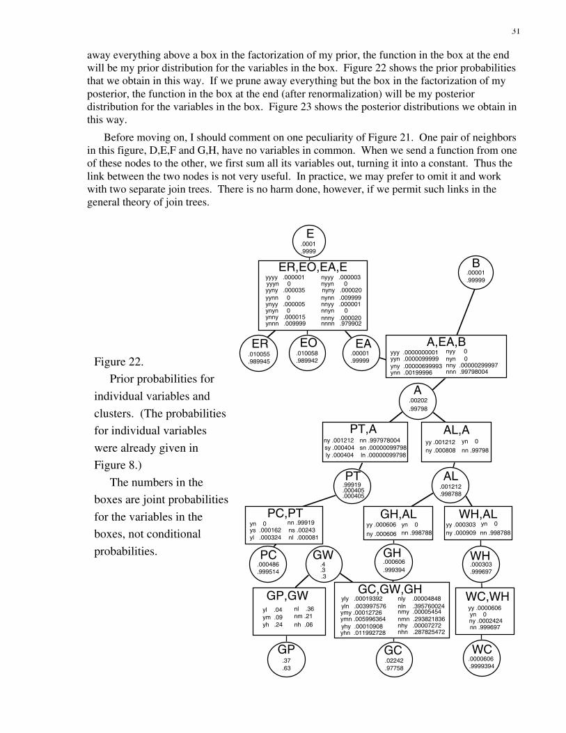
away everything above a box in the factorization of my prior, the function in the box at the endwill be my prior distribution for the variables in the box. Figure 22 shows the prior probabilitiesthat we obtain in this way. If we prune away everything but the box in the factorization of myposterior, the function in the box at the end (after renormalization) will be my posteriordistribution for the variables in the box. Figure 23 shows the posterior distributions we obtain inthis way.

Before moving on, I should comment on one peculiarity of Figure 21. One pair of neighborsin this figure, D,E,F and G,H, have no variables in common. When we send a function from oneof these nodes to the other, we first sum all its variables out, turning it into a constant. Thus thelink between the two nodes is not very useful. In practice, we may prefer to omit it and workwith two separate join trees. There is no harm done, however, if we permit such links in thegeneral theory of join trees.

Figure 22.

Prior probabilities for

individual variables and

clusters. (The probabilities

for individual variables

were already given in

Figure 8.)

The numbers in the

boxes are joint probabilities

for the variables in the

boxes, not conditional

probabilities.

E

A

ER,EO,EA,E

PT,A AL,A

WC,WH

PT AL

B

.0001

.9999

EAER EO

yyyy .000001yyyn 0yyny .000035yynn 0ynyy .000005ynyn 0ynny .000015ynnn .009999

nyyy .000003nyyn 0nyny .000020nynn .009999nnyy .000001nnyn 0nnny .000020nnnn .979902

P(a|ea,b)

A,EA,Byyy .0000000001yyn .0000099999yny .00000699993ynn .00199996

nyy 0nyn 0nny .00000299997nnn .99798004

ny .001212 nn .997978004sy .000404 sn .00000099798ly .000404 ln .00000099798

yy .001212 yn 0

ny .000808 nn .99798

P(pc|pt)PC,PT

yn 0 nn .99919ys .000162 ns .00243yl .000324 nl .000081

P(gh|al)GH,ALyy .000606 yn 0

ny .000606 nn .998788

P(wh|al)WH,AL yn 0yy .000303

ny .000909 nn .998788

GH WHPC GW

GP,GW

GPGP GC WC

yl .04ym .09yh .24

nl .36 nm .21nh .06

yy .0000606 yn 0ny .0002424 nn .999697

GC,GW,GHyly .00019392yln .003997576ymy .00012726ymn .005996364yhy .00010908yhn .011992728

nly .00004848nln .395760024nmy .00005454nmn .293821836nhy .00007272nhn .287825472

WC,WH

.010055

.989945.010058.989942

.00001

.99999

.00001

.99999

.00202

.99798

.001212

.998788

.000303

.999697

.0000606.9999394

.02242

.97758.37.63

.000486

.999514.4.3.3

.99919

.000405

.000405

.000606

.999394

32

Figure 23.

Posterior probabilities

for individual variables and

clusters. (The probabilities

for individual variables

were already given in

Figure 19.)

Again, the boxes contain

joint rather than conditional

probabilities.

EAER01

EO01

E

A

GP GC WC

P(a|ea,b)


nnyy .00051 nnny .00002nnnn .99947

yyy 5x10yyn .0005yny .0035ynn .9960

ny .79sy .16ly .05

ER,EO,EA,E

A,EA,B

PT,A AL,A

PC,PT GH,AL WH,AL

GC,GW,GH WC,WHGP,GW

GP GC WC01

10

10

GH WHPC01

GW

PT AL

B

.0005

.9995

yy 1.0

10

10

10

.79

.16

.05

.61

.31

.08

.98

.02

.003

.997

.0005

.9995

nn .79ns .16nl .05

yy .98ny .02

yy 1.0

yy 1.0yly .599 yln .007ymy .305 ymn .009yhy .075 yhn .005

nl .61nm .31nh .08

-9

When the Causal Structure is Not a Tree. The story of the burglar alarm, as I told it, hadthe causal structure of a tree (Figure 1) and led to a factorization whose clusters could be ar-ranged in a join tree (Figure 3). Most causal structures are not trees and lead to factorizationswhose clusters cannot be arranged in a join tree. In such a case, a join tree whose nodes containthe clusters will have some nodes that are larger than any of the clusters they contain.

To illustrate this point, let me return to the story of the burglar alarm and entertain areasonable objection to some of the conditional independence assumptions I made there. Iassumed that the three telephone calls are independent of the occurrence of an earthquake, giventhat the alarm does or does not go off. Yet Watson's call, which I could not understand, mighthave been about an earthquake rather than about my burglar alarm. Gibbons, who is a bit odd,

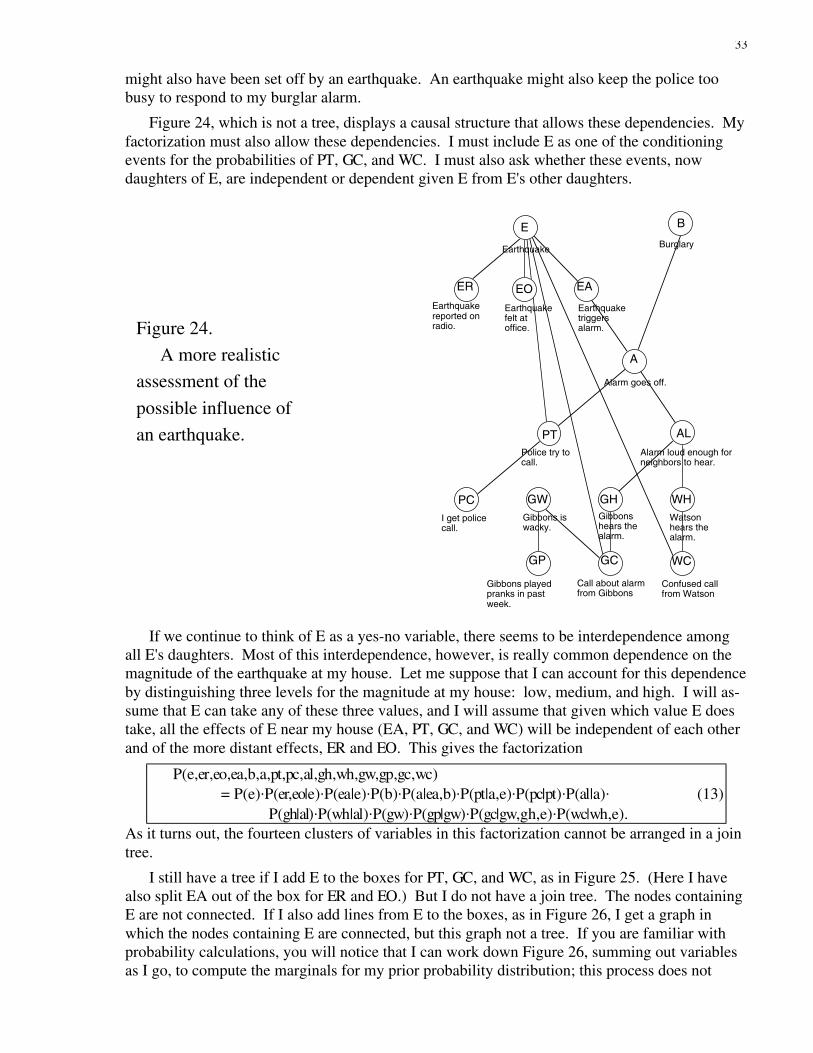
33

might also have been set off by an earthquake. An earthquake might also keep the police toobusy to respond to my burglar alarm.

Figure 24, which is not a tree, displays a causal structure that allows these dependencies. Myfactorization must also allow these dependencies. I must include E as one of the conditioningevents for the probabilities of PT, GC, and WC. I must also ask whether these events, nowdaughters of E, are independent or dependent given E from E's other daughters.

Figure 24.

A more realistic

assessment of the

possible influence of

an earthquake.

E B

ER EO EA

A

PT AL

PC GW GH WH

GP GC WC

Earthquake Burglary




Alarm goes off.


Police try to call.

I get policecall.

Gibbons is wacky.






If we continue to think of E as a yes-no variable, there seems to be interdependence amongall E's daughters. Most of this interdependence, however, is really common dependence on themagnitude of the earthquake at my house. Let me suppose that I can account for this dependenceby distinguishing three levels for the magnitude at my house: low, medium, and high. I will as-sume that E can take any of these three values, and I will assume that given which value E doestake, all the effects of E near my house (EA, PT, GC, and WC) will be independent of each otherand of the more distant effects, ER and EO. This gives the factorization

P(e,er,eo,ea,b,a,pt,pc,al,gh,wh,gw,gp,gc,wc)= P(e).P(er,eo|e).P(ea|e).P(b).P(a|ea,b).P(pt|a,e).P(pc|pt).P(al|a). (13)

P(gh|al).P(wh|al).P(gw).P(gp|gw).P(gc|gw,gh,e).P(wc|wh,e).As it turns out, the fourteen clusters of variables in this factorization cannot be arranged in a jointree.

I still have a tree if I add E to the boxes for PT, GC, and WC, as in Figure 25. (Here I havealso split EA out of the box for ER and EO.) But I do not have a join tree. The nodes containingE are not connected. If I also add lines from E to the boxes, as in Figure 26, I get a graph inwhich the nodes containing E are connected, but this graph not a tree. If you are familiar withprobability calculations, you will notice that I can work down Figure 26, summing out variablesas I go, to compute the marginals for my prior probability distribution; this process does not

34

depend on the graph being a tree. But if I want to compute my posterior probabilities for A,given my six observations, then Figure 26 will not help me. I need to prune twigs until only A isleft, and I cannot do this in a graph that is not a tree.

E B

ER EO EA

A

PT AL

PC GH WH

GP GC WC

P( er,eo | e )

P(a | ea,b)

P(gp | gw)

P(e) P(b)

P(al | a)


P(gc | gw,gh,e) P(wc | wh,e)

P(pt | a,e)

GWP(gw)

ER,EO,E

A,EA,B

PT,A,E AL,A

PC,PT GH,AL WH,AL

GC,GW,GH,E WC,WH,EGP,GW

P( ea | e )EA,E

E B

ER EO EA

A

PT AL

PC GH WH

GP GC WC

P( er,eo | e )

P(a | ea,b)

P(gp | gw)

P(e) P(b)

P(al | a)



P(pt | a,e)

GWP(gw)

ER,EO,E

A,EA,B

PT,A,E AL,A

PC,PT GH,AL WH,AL


P( ea | e )EA,E


In order to construct a join tree containing the clusters in (13), I must use some nodes largerthan the clusters they contain. Figure 27 shows one way of doing this. In this figure, I haveadded E not only to the boxes for PT, GC, and WC, as in Figure 25, but also to all the nodes be-tween these boxes and the Es at the top of the figure. Figure 27 is a join tree, and I can use it tocompute my posterior marginals. The computation will be more time-consuming than thecomputation in Section 2.4, for I must deal with three times as many terms (this is the size of E'sframe) when pruning any node to which E has been added. This is onerous but feasible. It is notlike working with 73,728 terms.

Because I started this section with Figure 3 rather than with the abstract idea of a join tree, Ihave made Figure 27 analogous to Figure 3. A more abstract point of view leads to a morestreamlined join tree. If I begin simply with the fourteen clusters in the factorization,

E ER,EO,E EA,E B A,EA,BPT,A,E PC,PT AL,A GH,AL WH,ALGW GP,GW GC,GW,GH,E WC,WH,E,

and I ask for the fewest and smallest nodes that contain these clusters and can be arranged in ajoin tree, then I will end up with these nodes:

ER,EO,E A,EA,B,E PT,A,E PC,PT AL,A,EGH,AL,E WH,AL,E GP,GW GC,GW,GH,E WC,WH,E.

This is only ten of the twenty-six nodes in Figure 27. Figure 28 shows one way of arrangingthese ten nodes in a join tree. It is more streamlined than Figure 27, but a close look at thecomputations involved in finding marginals will reveal that this streamlining does not cut down

35

on the computation. The extra nodes in Figure 27 serve only as storage in the course of thecomputation.

Figure 27.

A join tree for the

factorization (13).

Some of the boxes

in this tree contain E

even though it does not

occur in the functions

they contain.

E B

ER EO EA,E

A,E

PT AL,E

PC GH,E

GP GC WC

P( er,eo | e )

P(a | ea,b)

P(gp | gw)

P(e) P(b)

P(al | a)



P(pt | a,e)

GWP(gw)

ER,EO,E

A,EA,B,E

PT,A,E AL,A,E

PC,PT GH,AL,E WH,AL,E


P( ea | e )EA,E

WH,E

Figure 28.

A more streamlined

join tree for the same

factorization.

P(er,eo|e) P(a|ea,b)

P(gp | gw)

P(e) P(b)

P(al | a)P(pc | pt)

P(gh | al) P(wh | al)


P(pt | a,e)

P(gw)

ER,EO,E A,EA,B,E

PT,A,E AL,A,E

GH,AL,E WH,AL,E


P(ea|e)

PC,PT

36

It is only in the most fortunate cases that the clusters in a factorization can themselves be ar-ranged in a join tree. Usually, as in this example, we must use a join tree with some largernodes. By using nodes that are large enough, we can always find a join tree that will hold agiven factorization, because a single node containing all the variables constitutes a join tree. Butin order for the computation to be feasible, the join tree must have relatively small nodes.

I have not told you how to check whether a collection of clusters can be arranged in a jointree, how to arrange them in a join tree if this is possible, or how to enlarge them minimally if itis not possible. For some answers to these questions and many references, see Pearl (1988) orShafer and Shenoy (1988).

3. Axioms for Local ComputationWe can describe the process of local computation that we learned in the preceding section in

an abstract way, using general terms such as marginalization and combination instead of morespecific terms such as summing out and multiplication. As I will explain briefly in this section,this more abstract description can be formalized as a set of axioms. These axioms apply not onlyto probabilities but also to other calculi, including belief functions, that have been used tomanage uncertainty in expert systems.

The Setting for the Axioms. What do we need in the way of a formal setting in order to talkabout marginalization and combination?

First, we need variables and sets of variables. I will use upper case Latin letters—A, B, C,and so on—to represent variables. I will use lower case Greek letters—α, β, γ, and so on—to

represent sets of variables.

Next, we need objects that are analogous to probability distributions for sets of variables. Iwill call these objects valuations, and I will use lower case Latin letters—f, g, h, and so on, torepresent them. Each valuation is associated with a certain set of variables. In the probabilitycase, a valuation on a set of variables is a non-negative function on those variables. A valuationon the variables {A,B,C}, for example, is a non-negative function f(a,b,c). In other applicationsof our axioms, we might have rather different objects as valuations. In the belief-function case, avaluation on a set of variables is a belief function over these variables. In the case of a non-numerical probability calculus, a valuation on a set of variables might be an assignment of termssuch as “likely” or “unbelievable” to certain configurations or sets of configurations of thesevariables.

Next, we need a way of combining valuations to get other valuations. In the probability case,combination is simply multiplication, but in other cases we will have other rules of combination.Whatever the rule is, I will write f⊗g for the valuation that I get by combining the valuations f

and g. In general, the number of variables with which we are concerned grows as we combinevaluations. If f is a valuation on α and g is a valuation on β, then f⊗g will be a valuation on

α∪β. In the probability case, for example, when we combine a valuation f(a,b,c) on {A,B,C}

with a valuation g(b,d,e) on {B,D,E}, we get f(a,b,c).g(b,d,e), which is a valuation on{A,B,C,D,E}.

37

Finally, we need a way of marginalizing a valuation from one set of variables to a smaller setof variables. In the probability case, we do this by summing out variables; the result ofmarginalizing f(a,b,c,d) to {A,B} is the function ∑

c,d

f(a,b,c,d) ,

which is a function only of a and b—i.e., a valuation on {A,B}. In general, whenever f is a val-

uation on α and β is a subset of α, I will write f↓β for the result of marginalizing f from α to β.

To summarize, we need four concepts. First, in the background, we need the familiarconcept of a variable. Second, we need some concept of a valuation on a set of variables. Thirdwe need a concept of combination for valuations; we combine f on α and g on β to get f⊗g on

α∪β. Fourth, we need a concept of marginalization for valuations; we marginalize f from α to β

to get f↓β.

The Axioms. Only three axioms are needed in order to justify the method of local computa-tion that we learned in the preceding section:

Axiom 1. Commutativity and associativity of combination.Suppose f, g, and h are valuations.Then f⊗g = g⊗f, and f⊗(g⊗h) = (f⊗g)⊗h.

Axiom 2. Consonance of marginalization.Suppose f is a valuation on α, and suppose γ ⊆ β ⊆ α.

Then (f↓β)↓γ = f↓γ.Axiom 3. Distributivity of combination over marginalization.

Suppose f and g are valuations on α and β, respectively.

Then (f⊗g)↓α = f⊗(g↓α∩β).

These axioms were first formulated by Shenoy and Shafer (1990).

The Probability Case. It is easy to see that all three axioms are satisfied by probabilities.Axiom 1 is satisfied because multiplication is commutative and associative. Axiom 2 is satisfiedbecause when we sum variables out of a function, the order in which we sum them does notmake any difference; we can first sum out the variables that are not in β and then the ones that

are in β but not in γ, or we can sum out all these variables all at once. Axiom 3 is satisfied

because multiplication distributes over addition; if α={A,B,C} and β={B,D,E}, for example,

then

(f⊗g)↓α(a,b,c) = (f⊗g)↓{A,B,C}(a,b,c) = ∑d,e

[f(a,b,c).g(b,d,e)]

= [f(a,b,c)].[∑d,e

g(b,d,e)] = f(a,b,c) . g↓{B}(b)

= (f⊗(g↓{B}))(a,b,c) = (f⊗(g↓α∩β))(a,b,c).

I used all three of these axioms when I explained local computation for probabilities inSection 2. I talked explicitly only about distributivity, but I took commutativity and associativityfor granted, and I also took it for granted that I could sum variables out of a function in any orderI liked.

38

Other Examples. Even in the case where valuations are real-valued functions on the vari-ables, there are many other choices for ⊗ and ↓ that satisfy the axioms.

For example, keeping ⊗ as multiplication, we can take ↓ to be the operation of maximizing

out variables, rather than summing them out. This means, for example, that if f is a valuation on{A,B,C,D}, then f↓{A,B}(a,b) is given by maxc,d f(a,b,c,d) instead of ∑

c,d

f(a,b,c,d) .

This is useful if we have a probability distribution in factored form and we want to find theconfiguration with greatest probability. We simply maximize inwards in the join tree, just as wesummed inwards in Section 2. If we are summing and we keep summing until we have summedout even the variables in the last remaining node, we will get either 1, in the case of the prior, orK-1, in the case of the posterior. If we are maximizing and we keep maximizing, we will obtainthe maximum value of the product of the factors with which we are working. If we keep track,as we pass the maxima inwards, of the values of the variables at which these maxima areattained, we will also know at the end which configuration of variables gives the product thismaximum value. We find for example, that in the story of the burglar alarm, the configurationfor the variables

(E,ER,EO,EA,B,A,PT,PC,AL,GH,WH,GW,GP,GC,WC)with greatest prior probability is

(E=no, ER=no, EO=no, EA=no, B=no, A=no, PT=not at all, PC=no,AL=no, GH=no, WH=no, GW=low, GP=no, GC=no, WC=no),

with prior probability 0.38, while the configuration with greatest posterior probability is(E=no, ER=no, EO=no, EA=no, B=no, A=yes, PT=not at all, PC=no,AL=yes, GH=yes, WH=yes, GW=low, GP=no, GC=yes, WC=yes),

with posterior probability 0.47. For details on this kind of computation, see Shafer and Shenoy(1988).

Finding a most probable configuration is only one optimization problem in which theobjective function can be decomposed. There are many others, with both additive andmultiplicative decompositions. Methods which take advantage of such decompositions arereferred to broadly as “non-serial dynamic programming.” Since our axioms are satisfied wheneither addition or multiplication is used for combination and either minimization ormaximization is used to eliminate variables, the whole field of non-serial dynamic programmingcan be seen as another instance of these axioms. Much of what we know about join trees,incidentally, is due to workers in this field (Bertele and Brioschi 1972).

These possibilities (maximization or minimization for ↓ and addition or multiplication for ⊗)

also permit various non-probabilistic calculi for the assessment of evidence. If we use additivescores to weigh evidence against configurations, for example, then we can use minimization tomarginalize, on the grounds that a configuration (a,b,c), say, has a given weight of evidenceagainst it if (a,b,c,d,e) has that weight of evidence against it for every choice of d and e. Spohn(1990) has formulated a non-probabilistic calculus along these lines, which Shenoy (1989) hasanalyzed in the light of the three axioms.

Belief Functions. Shenoy and I were first led to the axioms stated above not by examples ofdirect probability computations like those in Section 2, but rather by examples from the theory ofbelief functions, an alternative theory of subjective probability on which I have worked for manyyears (Shafer 1976, 1990). The axioms are satisfied if we take valuations to be belief functions,

39

combination to be Dempster's rule, and marginalization to be the standard marginalization ofbelief-function theory.

I cannot go into details here; instead I must refer you to Shenoy and Shafer (1990). I do,however, want to point out that applications of belief functions do not usually begin with acausal structure such as that of Figure 1. Instead, we begin by sorting our evidence intoindependent items and formulating variables on which these items bear. The formal startingpoint for combination is therefore a set of belief functions bearing on different clusters ofvariables. Efficient combination requires that these clusters be arranged in a join tree. Thus jointrees are the natural setting for belief functions; here we do not need to navigate our way to jointrees from causal trees, as I did for probabilities in Section 2.

4. Artificial Intelligence and the Philosophy of ProbabilityWhat are the limits of probability? In what problems is probability useful and in what prob-

lems is it not? What other methods are useful when probability is not? An outsider might expectthat statisticians have systematically tried to answer this question. In fact, however, we do nothave a tradition of scholarly study of the limits of our subject. Traditionally, the foundations ofour subject have been dominated instead by the Bayesian vs. frequentist debate over how tointerpret and use probability.

I believe that AI can help broaden our perspective. It can teach us some alternatives toprobability, and it can help move the question of whether and how to use probability from theBayesian vs. frequentist debate to a broader context of choices.

The difference in perspective between AI and statistics lies primarily in AI's emphasis on im-plementation. As statisticians, we are accustomed to thinking in terms of models and methods;we see implementation as practically but not conceptually important. For workers in AI, likeother computer scientists, questions of implementation loom larger.

Workers in AI have two broad categories for the issues that arise in implementation:representation and control. In this section, I briefly relate representation and control to the use ofprobability. I argue that the problems in which probability can play a role in both representationand control lie at one extreme of a continuum. The axioms we have just studied represent onedirection for generalization of probability within this continuum.

Representation. From the AI point of view, whether knowledge can in principle be repre-sented in probabilistic terms is secondary to the question of how we actually represent thisknowledge in a computer program.

Bayesians argue that decisions are rational only if they maximize expected utility. Strictlyspeaking, this is not a claim about implementation; nothing is said about how the maximizationis to be achieved. But standard presentations of Bayesian decision theory, such as Raiffa (1968),spell out how the maximization can be achieved through the explicit assessment of probabilitiesand utilities. It is no surprise, therefore, that psychologists and workers in AI have seen theBayesian claim as a claim about implementation.

A number of authors have investigated whether people do make critical decisions byexplicitly assessing probabilities and utilities. The clear conclusion is that they do not. Peopledo sometimes deliberate in a way that refers to qualitative probabilities and utilities. But aspeople become experts, they pay less rather than more attention to probabilities. Experts do usetheir experience, which consists to some extent of frequencies, but this experience does not seem

40

to be compiled in their minds in the form of probabilities. How is it compiled? Some authors,such as Kuipers et al. (1988) have advanced the hypothesis that it is compiled in rules of thumb.Other, such as Klein (1989), hypothesize more complicated data structures. In many cases, anexpert seems to have a list of typical situations, ordered by their frequency of occurrence. Eachsituation has lists of expectations and recommended actions, also ordered by the frequency withwhich they are appropriate. Faced with a new situation, the expert checks through the list oftypical situations, looking for a match. Once a match is found, the expert then checks similarlythrough the list of recommended actions. The choice of a situation or an action from the listseems less a matter of deliberation than a matter of recognition.

An intelligent advocate of probability will point out that probability does not need to be theexplicit mode of representation in order to be of central importance. If we use Bayesian decisiontheory in order to derive a discriminant function, then we are using Bayesian decision theorywhen we use the discriminant function, even if we use it as a rule of thumb, withoutremembering how we derived it. The centrality of probability is not so clear, however, when wetry to understand how experience is stored in problems such as those studied by Klein. Theprinciple that we should list typical situations in our memory in order of frequency is only a firststep towards deciding how to organize experience into typical situations.

Control. As Paul R. Cohen (1987) has emphasized, the designers of robots and artificial in-telligence programs usually pay more attention to control, in the sense of computer science, thanto the explicit representation of uncertainty. When conflicting claims or conflicting evidenceimpinge on a system, the resolution is often determined by which subsystem has control—whichsubsystem says what to do next. Once rules for passing control have been established, the ex-plicit representation and weighing of conflicting evidence may be redundant.

I have just discussed one way in which frequency information can represented by a controlsystem rather than by probability numbers: we can list typical situations or typical actions inorder of frequency and then try them out in the order in which they are listed.

A more extreme case of managing uncertainty by control is provided by the robots designedby Rodney Brooks at MIT (Brooks 1986, Waldrop 1990). In these robots, individual simple-minded reflexes are organized hierarchically, with the inputs from different sensors beingdirected to levels where they are most relevant. The most elementary part of the system usessonar to wander without hitting obstacles. A higher level uses vision to decide when to interferewith the lower level in order to direct the robot towards a goal. Thus these two sources ofevidence, sonar and vision, are used by different parts of the system instead of being representedand compared or combined by some central processor. Experience is used to calibrate Brooks'srobots, and hence we can say that they use frequency information in some sense. It is difficult toargue, however, that probability is playing any role in representation or control within thesystem.

Probabilistic Expert Systems. The theory of Section 2 suggests an expert system that relieson probability for both representation and control. Experience is represented in the form ofnumerical probabilities, and control is provided by the structure of the tree. There are expert sys-tems that do use probability in this thorough-going way. The best example of this is probably theMUNIN expert system for diagnosing muscle and nerve diseases, developed in Denmark(Andreassen et al. 1987).

What are the characteristics of problems that lend themselves to such probabilistic expertsystems?

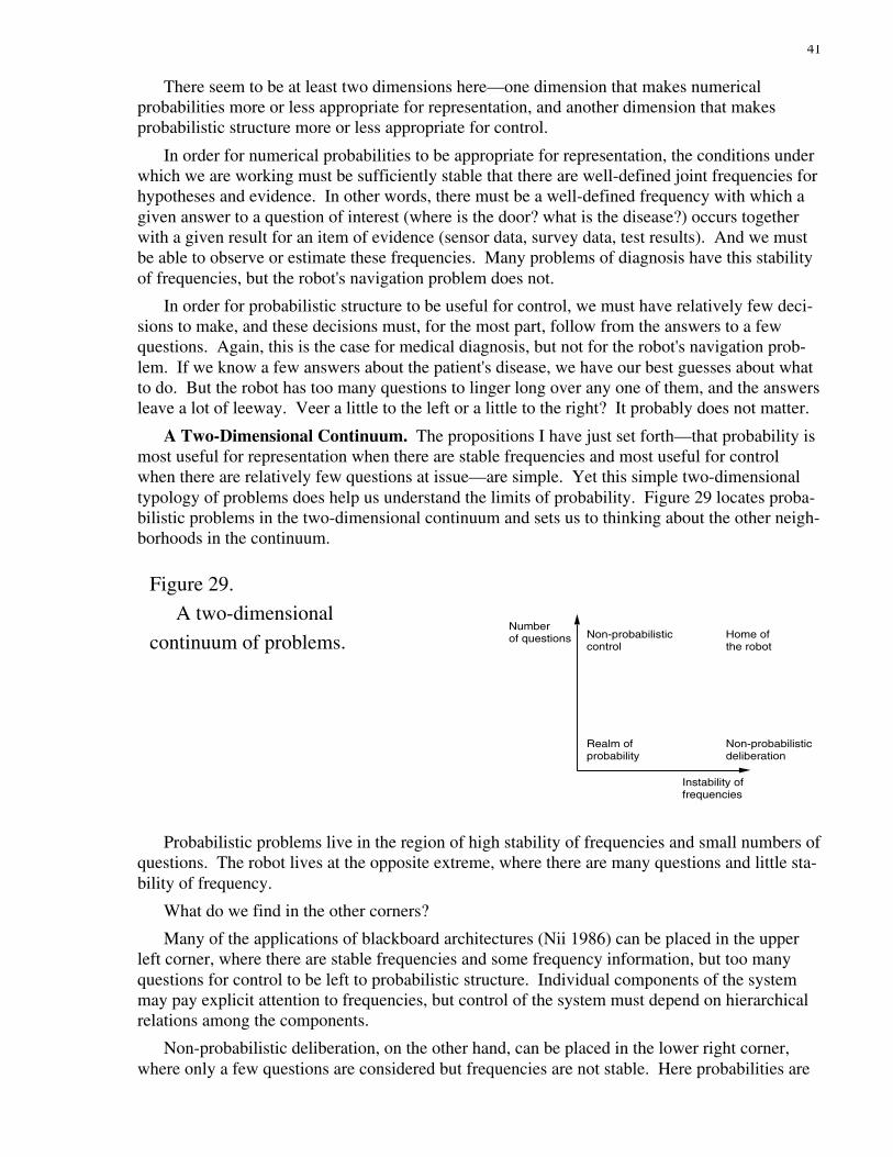
41

There seem to be at least two dimensions here—one dimension that makes numericalprobabilities more or less appropriate for representation, and another dimension that makesprobabilistic structure more or less appropriate for control.

In order for numerical probabilities to be appropriate for representation, the conditions underwhich we are working must be sufficiently stable that there are well-defined joint frequencies forhypotheses and evidence. In other words, there must be a well-defined frequency with which agiven answer to a question of interest (where is the door? what is the disease?) occurs togetherwith a given result for an item of evidence (sensor data, survey data, test results). And we mustbe able to observe or estimate these frequencies. Many problems of diagnosis have this stabilityof frequencies, but the robot's navigation problem does not.

In order for probabilistic structure to be useful for control, we must have relatively few deci-sions to make, and these decisions must, for the most part, follow from the answers to a fewquestions. Again, this is the case for medical diagnosis, but not for the robot's navigation prob-lem. If we know a few answers about the patient's disease, we have our best guesses about whatto do. But the robot has too many questions to linger long over any one of them, and the answersleave a lot of leeway. Veer a little to the left or a little to the right? It probably does not matter.

A Two-Dimensional Continuum. The propositions I have just set forth—that probability ismost useful for representation when there are stable frequencies and most useful for controlwhen there are relatively few questions at issue—are simple. Yet this simple two-dimensionaltypology of problems does help us understand the limits of probability. Figure 29 locates proba-bilistic problems in the two-dimensional continuum and sets us to thinking about the other neigh-borhoods in the continuum.

Figure 29.

A two-dimensional

continuum of problems.Numberof questions

Instability of frequencies

Realm ofprobability

Home of the robot

Non-probabilisticdeliberation

Non-probabilisticcontrol

Probabilistic problems live in the region of high stability of frequencies and small numbers ofquestions. The robot lives at the opposite extreme, where there are many questions and little sta-bility of frequency.

What do we find in the other corners?

Many of the applications of blackboard architectures (Nii 1986) can be placed in the upperleft corner, where there are stable frequencies and some frequency information, but too manyquestions for control to be left to probabilistic structure. Individual components of the systemmay pay explicit attention to frequencies, but control of the system must depend on hierarchicalrelations among the components.

Non-probabilistic deliberation, on the other hand, can be placed in the lower right corner,where only a few questions are considered but frequencies are not stable. Here probabilities are

42

not appropriate for representations of uncertainty, but other explicit representations, such asbelief functions, may be useful. I would place the most interesting applications of belieffunctions, including applications to financial auditing (Srivastava et al. 1989) in this corner.Belief functions are only one possibility for representation, however. As long as we are workingwith only a few central questions, the axioms of the preceding section may apply, and theseaxioms leave open the possibility of relying on the structure of the reasoning itself for control ofthat reasoning.

ReferencesAndreassen, S., M. Woldbye, B. Falck, and S.K. Andersen (1987). MUNIN—A causal proba-

bilistic network for interpretation of electromyographic findings. Proceedings of the TenthInternational Joint Conference on Artificial Intelligence, pp. 366-372.

Barwise, Jon, and John Perry (1983). Situations and Attitudes. MIT Press, Cambridge,Massachusetts.

Beeri, Catriel, Ronald Fagin, David Maier, and Mihalis Yannakakis (1983). On the desirabilityof acyclic database schemes. Journal of the Association of Computing Machinery 30 479-513.

Bertele, U., and Brioschi, F. (1972). Nonserial Dynamic Programming. Academic Press, NewYork.

Brooks, Rodney A. (1986). A robust layered control system for a mobile robot. IEEE Journal ofRobotics and Automation RA-2(1). Reprinted in Shafer and Pearl (1990), pp. 204-214.

Bundy, Alan (1983). The Computer Modelling of Mathematical Reasoning. Academic Press.Cohen, Paul R. (1987). The control of reasoning under uncertainty: A discussion of some pro-

grams. The Knowledge Engineering Review 2(1). Reprinted in Shafer and Pearl (1990), pp.177-197.

David, Edward E., Jr., et al. (1984) Renewing U. S. Mathematics: Critical Resources for theFuture. (Ad Hoc Committee on Resources for the Mathematical Sciences, National ResearchCouncil) Notices of the American Mathematical Society 31:5 434-466.

Davis, Philip J., and Reuben Hersh (1986). Descartes' Dream: The World According toMathematics. Harcourt Brace Jovanovich, San Diego.

Duncan, Otis Dudley (1975). Introduction to Structural Equation Models. Academic Press,New York.

Farlow, Stanley J. (1984). Self-Organizing Methods in Modeling. Marcel Dekker, New Yorkand Basel.

Gardner, Howard (1985). The Mind's New Science: A History of the Cognitive Revolution.Basic Books, New York.

Geiger, Dan (1990). Graphoids: A qualitative framework for probabilistic inference. TechnicalReport R-142, Cognitive Systems Laboratory, Computer Science, UCLA.

Kac, Mark, Gian-Carlo Rota, and Jacob T. Schwartz (1986). Discrete Thoughts: Essays onMathematics, Science, and Philosophy. Birkhauser, Boston.

Klein, Gary A. (1989). Recognition-primed decisions. Advances in Man-Machines SystemsResearch 5 47-92.

Kuipers, Benjamin, Alan J. Moskowitz, and Jerome P. Kassirer (1988). Critical decisions underuncertainty: representation and structure. Cognitive Science 12 177-210. Reprinted inShafer and Pearl (1990), pp. 105-121.

Lauritzen, Steffen L., and David J. Spiegelhalter (1988). Local computations with probabilitieson graphical structures and their application to expert systems (with discussion). Journal of

43

the Royal Statistical Society, Series B 50 157-224. Reprinted in Shafer and Pearl (1990), pp.415-448.

Maier, David (1983). The Theory of Relational Databases. Computer Science Press, Rockville,Maryland.

McAllester, David A. (1989). ONTIC: A Knowledge Representation System for Mathematics.MIT Press, Cambridge, Massachusetts.belief networks. Artificial Intelligence 29 241-288.

Nii, H.P. (1986). The blackboard model of problem solving. AI Magazine 7(2) 38-54.Pearl, Judea (1988). Probabilistic Reasoning in Intelligent Systems: Networks of Plausible

Inference. Morgan Kaufmann, San Mateo, California.Raiffa, Howard (1968). Decision Analysis. Addison-Wesley, Reading, Massachusetts.Shafer, Glenn (1976). A Mathematical Theory of Evidence. Princeton University Press.Shafer, Glenn (1990). Perspectives on the theory and practice of belief functions. To appear in

International Journal of Approximate Reasoning.Shafer, Glenn, and Judea Pearl (1990). Readings in Uncertain Reasoning. Morgan Kaufmann,

San Mateo, California.Shafer, Glenn, and Prakash Shenoy (1988). Local computation in hypertrees. Working Paper

No. 201, School of Business, University of Kansas.Shafer, Glenn, and Prakash Shenoy (1990). Probability propagation. Annals of Mathematics

and Artificial Intelligence 2 327-352.Shenoy, Prakash P. (1989). On Spohn's rule for revisions of beliefs. Working Paper 213, School

of Business, University of Kansas.Shenoy, Prakash P., and Glenn Shafer (1986). Propagating belief functions using local computa-

tions. IEEE Expert 1(3) 43-52.Shenoy, Prakash P., and Glenn Shafer (1990). Axioms for probability and belief-function

propagation. Uncertainty in Artificial Intelligence 4, pp. 169-198. R.D. Shachter, T.S.Levitt, L.N. Kanal, and J.F. Lemmer, eds. North-Holland. Reprinted in Shafer and Pearl(1990), pp. 575-610.

Spohn, Wolfgang (1990). A general non-probabilistic theory of inductive reasoning.Uncertainty in Artificial Intelligence 4. R.D. Shachter, T.S. Levitt, L.N. Kanal, and J.F.Lemmer, eds. North-Holland.

Srivastava, Rajendra P., Prakash P. Shenoy, and Glenn Shafer (1989). Audit risk: A belief-function approach. Working Paper 212, School of Business, University of Kansas.

Waldrop, M. Mitchell (1990). Fast, cheap, and out of control. Science 248 959-961.White, Halbert (1989). Some asymptotic results for learning in single hidden-layer feedforward

network models. Journal of the American Statistical Association 84 1003-1013.

why should statisticians be interested in artificial ... · why should statisticians be interested...

Documents