why are gambling markets organised so differently …aldous/157/papers/levitt_gambling... · why...

WHY ARE GAMBLING MARKETSORGANISED SO DIFFERENTLYFROM FINANCIAL MARKETS?*

Steven D. Levitt

The market for sports gambling is structured very differently from the typical financial market.In sports betting, bookmakers announce a price, after which adjustments are small and in-frequent. Bookmakers do not play the traditional role of market makers matching buyers andsellers but, rather, take large positions with respect to the outcome of game. Using a uniquedata set, I demonstrate that this peculiar price-setting mechanism allows bookmakers to achievesubstantially higher profits. Bookmakers are more skilled at predicting the outcomes of gamesthan bettors and systematically exploit bettor biases by choosing prices that deviate from themarket clearing price.

There are many parallels between trading in financial markets and sportswagering. First, in both settings, investors with heterogeneous beliefs andinformation seek to profit through trading as uncertainty is resolved over time.Second, sports betting, like trading in financial derivatives, is a zero-sum gamewith one trader on each side of the transaction. Finally, large amounts ofmoney are potentially at stake. The four major British bookmaking firms reportturnover of almost £10 billion in 2002; estimates of wagering on sporting eventsin the US go as high as $380 billion annually (National Gambling Impact StudyCommission, 1999).

In light of these similarities, it is surprising that these two types of markets areorganised so differently. In most financial markets, prices change frequently.The prevailing price is that which equilibrates supply and demand. The primaryrole of market makers is to match buyers with sellers. With sports wagering andalso horse racing in the UK, market makers (i.e. bookmakers) simply announcea ‘price’ (which can be odds to win a horse race, or for sporting events can beodds to win a game or a point spread, e.g., the home team to win an Americanfootball game by at least 3.5 points), after which adjustments are typically smalland relatively infrequent.1 If that price is not the market clearing price, then the

* I thank John Cochrane, Stefano DellaVigna, Roland Fryer, Lars Hansen, Stephen Machin, CaseyMulligan, Koleman Strumpf, Justin Wolfers and seminar participants at the Royal Economic Societyannual conference and University of California-Berkeley for helpful discussions and comments. I alsogratefully acknowledge Casey Mulligan and Koleman Strumpf for providing some of the data used inthis paper. Trung Nguyen provided excellent research assistance. Portions of this paper were writtenwhile the author was a Spencer Foundation fellow at the Center for Advanced Studies of BehavioralSciences. This research was funded by a grant from the National Science Foundation.

1 In my data on American football, in the five days preceding a game, the posted price changes anaverage of 1.4 times per game. When the price does change, in 85% of the cases the line moves by theminimum increment of one-half of a point. Thus, the posted spread on Tuesday is within one point ofthe posted spread at kickoff on Sunday in 90% of all games. These calculations are based on infor-mation on changes in the casino lines reported at http://www.wagerline.com. In horse racing, the oddsset by bookmakers change more frequently.

The Economic Journal, 114 (April), 223–246. � Royal Economic Society 2004. Published by BlackwellPublishing, 9600 Garsington Road, Oxford OX4 2DQ, UK and 350 Main Street, Malden, MA 02148, USA.

[ 223 ]

bookmakers may be exposed to substantial risk.2 If bettors are able to recogniseand exploit mispricing on the part of the bookmaker, the bookmaker can sus-tain large losses. The risk borne by bookmakers on sports betting is categoricallydifferent from the casino’s risk on other games of chance such as roulette, keno,or slot machines. In those games of chance, the odds are stacked in favour ofthe casino and the law of large numbers dictates profits for the house. Incontrast, however, if the bookmaker sets the wrong line on sporting events, itcan lose money, even in the long run. The presence of a small number ofbettors whose skills allow them to achieve positive expected profits could provefinancially disastrous to the bookmaker. Such bettors could either amass largebankrolls or, in the presence of credit constraints, sell their information toothers.

Although the mechanism used for price-setting in sports betting seems peculiar,there are at least three scenarios in which the bookmaker can sustain profitsimplementing it. In the first scenario, bookmakers are extremely good at deter-mining in advance the price which equalises the quantity of money wagered oneach side of the bet. If this occurs, the bookmaker makes money regardless of whowins the game since the bookmaker charges a commission (known as the ‘vig’) onbets.3 Following this strategy, bookmakers do not have to have any particular skillin picking the actual outcome of sporting events, they simply need to be good atforecasting how bettors behave. Popular depictions of bookmaker behaviour havestressed this explanation.4

An alternative scenario under which this price-setting mechanism could persistis if bookmakers are systematically better than gamblers in predicting the out-comes of games. If that were the case, the bookmaker could set the ‘correct’ price(i.e. the one which equalises the probability that a bet placed on either side of awager is a winner). Although the money bet on any individual game would not beequalised, on average the bookmaker will earn the amount of the commission

2 There are many notorious examples of bookmakers suffering large losses. It is reported that overhalf of all British bookmakers were bankrupted when Airborne won the Epsom Derby in 1946 (thefirst running after World War II ended) at odds of 50 to 1 (Smith, 2002). In 1996, popular jockeyFrankie Dettori won seven straight races, costing bookmakers an estimated £30 million (GamblingMagazine, 1999). Coral Eurobet reported losses of £12 million on internet betting in quarter-finalround of Euro 2000 soccer championship (Smith, 2002).

3 Typically, bettors must pay the casino 110 units if a bet loses, but are paid only 100 units if the betwins.

4 For instance, a website devoted to educating novice gamblers (http://www.nfl-betting.org) writes,‘A sports bettor needs to realize that the point spread on a game is NOT a prediction by an odds makeron the outcome of a game. Rather, the odds are designed so that equal money is bet on both sides of thegame. If more money is bet on one of the teams, the sports book runs the risk of losing money if thatteam were to win. Bookmakers are not gamblers – they want to make money on every bet regardless ofthe outcome of the game.’ Similarly, Lee and Smith (forthcoming) write, ‘Bookies do not want theirprofits to depend on the outcome of the game. Their objective is to set the point spread to equalize thenumber of dollars wagered on each team and to set the total line to equalize the number of dollarswagered over and under. If they achieve this objective, then the losers pay the winners $10 and pay thebookmaker $1, no matter how the game turns out. This $1 profit (the ‘‘vigorish’’) presumably com-pensates bookmakers for making a market and for the risk they bear that the point spread or total linemay be set incorrectly.’

224 [ A P R I LT H E E C O N O M I C J O U R N A L

� Royal Economic Society 2004

charged to the bettors. Unlike the first scenario above, however, if prices are set inthis manner, the bookmaker will lose if gamblers are actually more skilled indetermining the outcome of games than is the bookmaker. The third possiblescenario combines elements of the two situations described in the precedingparagraphs. If bookmakers are not only better at predicting game outcomes butalso proficient at predicting bettors preferences, they can do even better inexpectation than to simply collect the commission. By systematically setting the‘wrong’ prices in a manner that takes advantage of bettor preferences, bookmakerscan increase profits. For instance, if bookmakers know that local bettors preferlocal teams, they can skew the odds against the local team. There are constraintson the magnitude of this distortion, however, since bettors who know the ‘correct’price can generate positive returns if the posted price deviates too much from thetrue odds.5

In this paper, I attempt to understand the structure of the market for sportsgambling better by exploiting a data set of approximately 20,000 wagers on theNational Football League, the premier league of American football placed by285 bettors at an online sports book as part of a high-stakes handicappingcontest. Two aspects of this data set are unique. First, in contrast to previousstudies of betting that only had information on prices, I observe both prices andquantities of bets placed. That information allows me to determine whether thebookmaker appears to be equalising the amount of bets on each side of awager. Second, I am able to track the behaviour of individual bettors over time,which provides a means of determining whether some bettors are more skillfulthan others. Although my data are from one bookmaker, the patterns observedhere are likely to generalise since all bookmakers offer nearly identical spreadson a given game.

A number of results emerge from the analysis. First, I demonstrate that thebookmaker does not appear to be trying to set prices to equalise the amount ofmoney bet on either side of a wager. In almost one-half of all games, at least two-thirds of the bets fall on one side of the gamble. Moreover, the spread chosensystematically fails to incorporate readily available information (e.g. which team isthe home team) that would help in equalising the money bet on either side of awager.6 For instance, in games where the home team is an underdog, on averagetwo-thirds of the wagers are on the visiting team. These findings argue stronglyagainst the first scenario presented above and the popular depictions of book-maker behaviour. A rationale for this failure to equalise the money emerges in the

5 This assumes that bookmakers are unable to offer different prices to different bettors. Indeed,there is evidence that local bookmakers who deal repeatedly with the same clients are able to exercisesome degree of price discrimination. See Strumpf (2002) for empirical evidence that bookmakers bothshade the odds against the home team and offer different odds to bettors with different past bettinghistories.

6 Of course, it is not the number of bets on either side of a wager that the bookmaker wants toequalise, but rather, the total dollars bet on either side. In my data, however, all wagers are constrainedto have the same dollar value, so the two are equivalent. If there are large bankroll bettors outside mysample who systematically bet against the prevailing sentiment of other bettors, conclusions based onmy sub-sample may be erroneous.

2004] 225W H Y G A M B L I N G M A R K E T S A R E R U N D I F F E R E N T L Y


paper’s second finding: bookmakers appear to be strategically setting prices inorder to exploit bettors’ biases, just as DellaVigna and Malmendier (2003) dem-onstrate health clubs do with their clients. Bettors exhibit a systematic bias towardfavourites and, to a lesser extent, towards visiting teams.7 Consequently, thebookmakers are able to set odds such that favourites and home teams win less than50% of the time, yet attract more than half of the betting action. By choosing theseprices, it appears bookmakers increase their gross profit margins by 20–30% over aprice-setting policy that attempts to balance the amount of money on either side ofthe wager. On the dimension of favourites versus underdogs, bookmakers appearto have distorted prices as much as possible without allowing a simple strategy ofalways betting on underdogs to become profitable. The fact that home teams andunderdogs cover the spread a disproportionate share of the time has been wellestablished in the literature (Golec and Tamarkin, 1991; Gray and Gray, 1997). Myfindings provide an explanation for that empirical regularity: it is profit maxim-ising for the bookmaker who sets the spread. Third, there is little evidence thatthere are individual bettors who are able to beat the bookmaker systematically.8

The distribution of outcomes across bettors is consistent with data randomlygenerated from independent tosses of a 50-50 coin. Moreover, how well a bettorhas done up to a certain point in time has no predictive value for future per-formance. Finally, the evidence is mixed as to whether aggregating bettor pref-erences has any predictive value in helping to beat the spread. In my sample, thereis some weak and ultimately statistically insignificant, evidence that bettors aremore likely to predict correctly when there is agreement among them as to whichteam looks attractive. Altogether, the results are consistent with the conclusionthat the bookmakers are at least as good at predicting the outcomes of games thanare even the most skilled gamblers in the sample and the bookmakers exploit theiradvantage by strategically setting prices to achieve profits that are likely higherthan would be possible if they simply acted as market makers letting supply anddemand equilibrate prices.

The remainder of the paper is organised as follows. Section 1 provides somebackground on wagering on professional football in the US. Section 2 describesthe data set used in the paper. Section 3 presents the empirical findings. Section 4concludes.

1. Background on American Football Wagering

American football is the most popular sport for wagering in the US, generating40% of sports-betting revenue for legal bookmakers in Nevada (Nevada GamingControl Board, 2002). USA Today reports that half of all Americans have a wager on

7 This finding is not to be confused with the bias towards longshots that has been observed inparimutuel horse-race betting (Ali, 1977; Golec and Tamarkin, 1998; Jullien and Salanie, 2000; Shin,1991, 1992, 1993; Thaler and Ziemba, 1988; Vaughan Williams and Paton, 1997). In football, the oddsare set to make the chance of each team covering the spread about 50%, making this considerationirrelevant.

8 While only tangentially related to the issues addressed in this paper, it is worth noting that there isan extensive academic literature devoted to the question of testing for market efficiency in wageringmarkets (Asch et al., 1984; Sauer et al., 1988; Woodland and Woodland, 1994; Zuber et al., 1985).



the outcome of the Super Bowl. The most common type of bet in pro footballinvolves picking the winner of a game against a point spread (a so-called ‘straightbet’).9 For instance, if the casino posts a betting line with the home team favouredby 3 points, a bettor can choose either (1) the home team to win by more than thatamount, or (2) the visiting team to either lose by less than three points or to winoutright. In the event the game ends exactly on the point spread, all bets arerefunded. Regardless of which team is chosen, the bettor typically pays the casino110 units if they lose the bet and collects 100 units when victorious. The differencein the amount paid on a loss versus the amount won for a victory is the casino’scommission, known as the ‘vig’. Because the bettor can take either side of thewager at the same payout rate, the casino needs to pick a betting line that roughlyequalises the probability of the two events occurring (in this case home teamwinning by more than three or more points, or failing to do so). The bettorreceives the spread in force at the time a wager is placed, regardless of lateradjustments made by the bookmaker.

Define terms as follows: p is the probability that the favourite wins a particulargame, f is the fraction of the total dollars bet on the game that go to the favourite,and v is the vig or commission charged by the bookmaker, which is paid only onlosing bets.10 The bookmaker’s expected gross profit per unit bet11 is given by

E(Bookmaker profit) ¼ ½ð1 � pÞf þ pð1 � f Þ�ð1 þ vÞ � ½ð1 � pÞð1 � f Þ þ pf �: ð1Þ

The terms inside the left set of brackets is the fraction of dollars bet in which thebookmaker wins. That amount is multiplied by 1 + v to reflect the bookmakers vig.The terms in the right set of brackets are the cases in which the bookmaker losesand has to payout to the bettor. Rearranging terms, (1) simplifies to

E(Bookmaker profit) ¼ ð2 þ vÞðf þ p � 2pf Þ � 1: ð2Þ

If either the probability the two teams win is equal (p ¼ 0.5) or the money bet onboth teams is equal (f ¼ 0.5), the bookmakers gross profit simplifies to v/2. Ineither of these instances, the bookmaker is indifferent about the outcome of thegame and earns a profit proportional to the size of the commission charged. Asnoted in the introduction, therefore, the bookmaker does not need to be able topredict the outcome of the games more accurately than the bettors to ensure aprofit. The bookmaker just needs to be able to predict bettor preferences so as tobalance out the money on each side of the wager.

9 There are many other types of bets available. For instance, one can bet on whether the total numberof points scored in a game is above or below a certain level. One can also bet on which team will win thegame (not against the spread), with the payouts appropriately adjusted to reflect the probability of theseoutcomes. It is also possible to parlay bets on a series of games such that the bettor receives a largepayout if correctly picking all the games and receives zero otherwise. Because my data only cover straightbets, I do not focus on these other bet types. Woodland and Woodland (1991) argue that the use ofpoint spreads as opposed to odds that depend only on which teams wins or loses is a bookmaker profit-maximising response to risk aversion on the part of bettors.

10 I define the model in terms of favourites and underdogs simply because this is the most salientdimension empirically. Game outcomes could be characterised along any relevant set of dimensions.

11 For simplicity, I treat the number of wagers placed as fixed in the analysis. To the extent thatchanging the odds affects the total volume of bets, the bookmaker’s overall gross profit would be afunction of both the number of bets and the gross profit per unit bet.



Equations (1) and (2) take f and p as given. Of course, the fraction of money beton the favourite will be a function of the probability the favourite actually wins, i.e.f ¼ f(p), with ¶f/¶p > 0.12 Taking the derivative of (2) with respect to p, an op-timising bookmaker will set p such that

½1 � 2f ðpÞ� þ ð1 � 2pÞ@f =@p ¼ 0: ð3Þ

The term in brackets is the benefit the bookmaker would achieve from distortingthe odds if gamblers did not respond to changes in prices. The remaining termcaptures the impact on profits of the behavioural response of bettors who switchtowards the team with better odds. Note that if bettors’ preferences are unbiased inthe sense that f(p ¼ 0.5) ¼ 0.5, then the bookmaker’s optimum is to choosep ¼ 0.5, which implies f ¼ 0.5 as well.

If, on the other hand, bettors’ preferences are biased so that f(p ¼ 0.5) > 0.5, asis true empirically in the data set, then the bookmaker can increase profits byreducing p below 0.5 (Kuypers (2000) makes this same point).13 Intuitively, ifbettors prefer favourites at fair odds, the bookmaker can offer odds slightly worsethan fair on favourites and still attract more than half of the wagers on thefavourite, yielding profits that are strictly higher than is the case at p ¼ 0.5.Mathematically, at p ¼ 0.5, the term in brackets in (3) is negative but the otherterm on the left-hand-side is equal to zero, demonstrating that the bookmaker isnot at an optimum. The bookmaker will not want to push p too far away from 0.5for two reasons, however. First, as p diverges from 0.5, it becomes increasinglycostly to the bookmaker when a bettor switches from the favourite to the under-dog. This is because the bet on the favourite is at (increasingly) unfair odds,whereas the bet on the underdog is at (increasingly) better than fair odds. Notethat when p is lowered to the point where f(p) ¼ 0.5, gross profits are back to thelevel attained when p ¼ 0.5. Thus, the bookmaker would never want to distortprices to that point. The second reason that the bookmaker cannot distort pricestoo much is that if some subset of bettors do not have biased preferences, thosebettors can exploit the distorted prices. With the standard vig, a bettor must win52.4% of bets to make profit.14 One could imagine that the volume of capitalavailable to bettors with positive expected profits could be enormous, both becausetheir bankrolls would grow over time and because the availability of such profitswould attract new investors. Thus, it would be surprising to observe pricedistortions so large that simple strategies (e.g. always bet the underdog) couldyield a positive profit.

The discussion above assumes that bookmakers have some market power. In aperfectly competitive market, ¶f/¶p will be near infinity and competition will drive

12 Throughout this analysis, I treat v (the commission charged by the bookmaker) as a parameterrather than a decision variable for the bookmaker. Commissions are virtually always 10%. Gaining abetter understanding of the reasons for the uniformity of commissions across bookmakers and overtime presents an interesting puzzle for future research.

13 Although I use the term ‘bias’ to describe bettor preferences, I do not necessarily imply irra-tionality on their part. If there is more consumption value associated with betting on favourites, thenbettor preferences for favourites could be completely rational.

14 A bettor breaks even when p ) (1 + v)(1 ) p) ¼ 0. The solution to that expression is p ¼ 0.5238.



the spread back to the point where f(p) ¼ 0.5 and no excess profits are obtained bybookmakers. Empirically, competitive pressure does not appear to be strongenough to eliminate excess profits. Understanding why this is the case is animportant unanswered question of this research.

2. The Data Set

The data used in this paper are wagers placed by bettors as part of a handicappingcontest offered at an online sports book during the 2001–2 NFL season. In thecontest, bettors were required to pick five games per week against the spread foreach of the 17 weeks of the NFL regular season (a total of 85 games). Bettors couldchoose those five games from any of the 13–15 games being played in a given week.One point was given for each correct pick, and one-half point if a game endedexactly on the spread. The entry fee was $250 per person, and there were 285entrants. All of the entry fees were returned as prize money, so participants werecompeting for a total pool of $71,250.15 60% (or $42,750) went to the bettor withthe most correct picks. Second to fifth place finishers received declining sharesof the pool. The last-place finisher (conditional on making 85 picks) received 5%of the pool. In the data, I observe the ID number of each bettor, all wagers placedas part of this contest, the spread at which the bet was placed and the outcome ofthe game.

There are a number of potential shortcomings with these data. First, these arenot wagers in the traditional sense. The bettor does not receive a direct payofffrom winning any particular game; the payoff is only based on the cumulativenumber of wins. Nonetheless, the presence of large monetary rewards to thewinners provides strong incentives to the participants. Presumably, the picksmade by bettors in the contest closely parallel the actual betting wagers theywere making; anecdotally that is true among the contest participants known tothe author.16 Second, the nature of the data make it impossible to ascertain theintensity of preferences across games since all selections receive equal weighting.Bettors may have much stronger preferences for their most favoured pick of theweek than would be the case for the fifth-favourite pick. Third, there is sub-stantial attrition in the sample. Of the 285 bettors who entered the contest, 100(a little more than one-third) made their entries all 17 weeks of the season.More than 60% participated in at least 15 of the 17 weeks of the season. Lessthan 10% of the contestants recorded data for fewer than eight weeks. Forbettors in the middle of the pack as the season progresses, the incentive tocontinue participating decreases substantially. Bettors who miss a week receivezero points, greatly reducing their likelihood of winning the contest, and

15 The apparent purpose of the contest was to ensure that the bettors had a reason to visit the websiteeach week. The fact that the worst-place finisher (conditional on having bet each week) received apayoff, reinforces this point.

16 One important way in which the contest wagers might be expected to differ from actual wagersplaced is that there is an incentive in the contest to pick outcomes that the bettor believes will beunpopular with other gamblers. That is because of the tournament structure of the contest in whichrewards are great in the extreme right-hand tail but no differentiation is made elsewhere in thedistribution.



disqualifying themselves from eligibility for the last-place prize. It should benoted, however, that attrition in this context adversely affects my ability to testonly one of the hypotheses: what the overall distribution of bettor success rateslooks like. Because attrition is non-random, the set of bettors who continue tothe end will be skewed. Fourth, the spreads used in the handicapping contestare fixed on the Tuesday preceding the game and do not fluctuate with theactual spread, even though a bettor’s contest picks are not due until the Fridaybefore the game. As a consequence, in some games, the actual spread and thecontest spread differ at the time an entry is made. All of the results of the paper,however, are robust to dropping games in which there are substantial fluctua-tions in the spread between Tuesday and Friday. Finally, these data are not theuniverse of bets placed at the sports book (although they are the universe ofbets in this contest), much less at sports books in general. Nor, as discussedbelow, are the bettors who participated in the contest likely to be a randomsubset of all bettors.

On the other hand, these data do offer enormous advantages over that whichis typically available. Virtually all previous analyses of sports wagering have fo-cused exclusively on prices but have not had access to any information aboutthe quantity of bets on each side of the wager (Avery and Chevalier, 1999;Golec and Tamarkin, 1991; Gray and Gray, 1997; Kuypers, 2000).17 In mysample, there are a total of 19,770 bets in the data set covering 242 differentgames. An average of 80.5 different bettors make a selection on a game, withthe minimum and maximum number of bets on a game ranging from 28 to146. Although the bettors included in my sample are not a random selection ofall gamblers, they represent a particularly interesting subset. These bettors arelikely to be relatively sophisticated, serious bettors. Because they are betting atan online sports book, they are likely to be geographically quite diverse. Insigning up for the contest, they are indicating an expectation that they plan tovisit (and presumably bet at) the internet sports book every week of the season.In addition, to the extent there are differences in skill across bettors, thiscontest should attract the most skilful players because it rewards exceptionallong-run performance.

3. Empirical Results

I begin the analysis by addressing the issue of whether the spread is set so as toequalise the wagers on either side, as well as testing the predictions of a model ofprofit-maximising bookmakers who exploit biases on the part of bettors. Theanalysis then turns to the question of whether bettors differ in their skill at pickingwinners. Finally, I examine whether aggregating information across bettors pro-vides any valuable information.

17 In his innovative work, Strumpf (2002) does have actual bets based on seized bookmaker records.Although his data are extremely informative on a number of questions, they are less than ideal for thequestions posed in this paper both because they cover a short time period and are geographicallylocalised.



3.1. How Are Prices Set?

The first question addressed is whether bookmakers set prices so as to equalise theamount of money on either side of the wager. Although I have data for only onebookmaker, it is important to note that the prices (i.e. spreads) offered by thissports book are virtually identical to those at any bookmaker online or at Las Vegascasinos. Thus, in practice individual bookmakers are not actively setting prices but,rather, following the lead of a handful of influential odds makers who are paid bylarge Las Vegas casinos for their services.

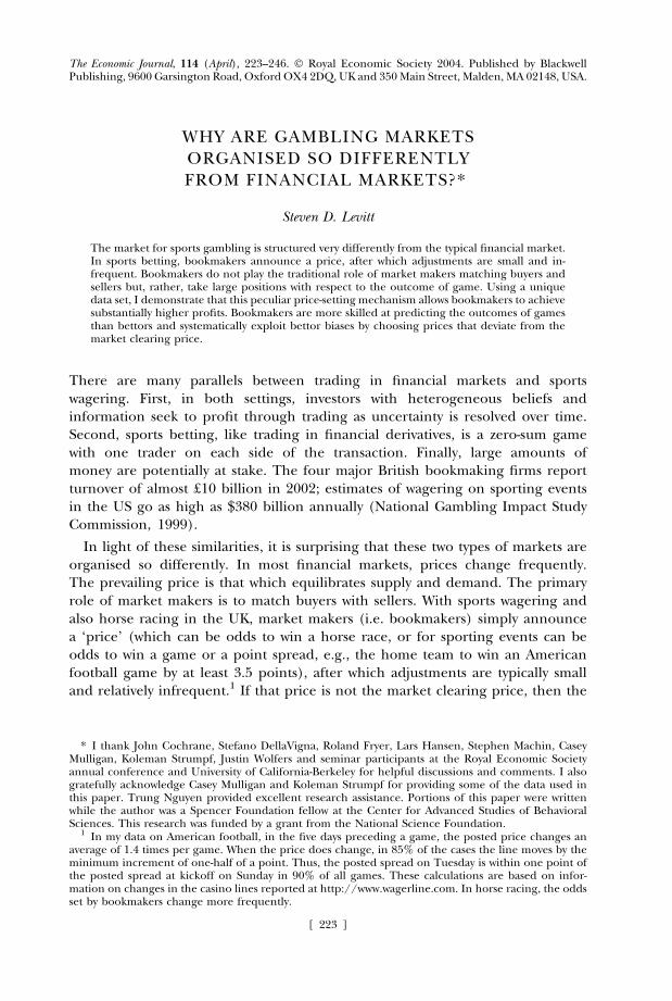
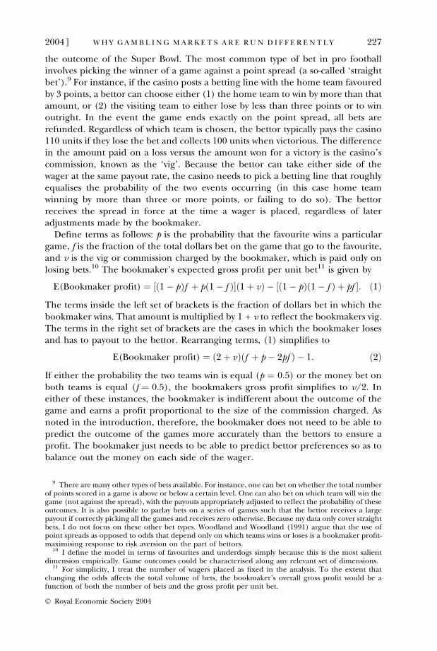
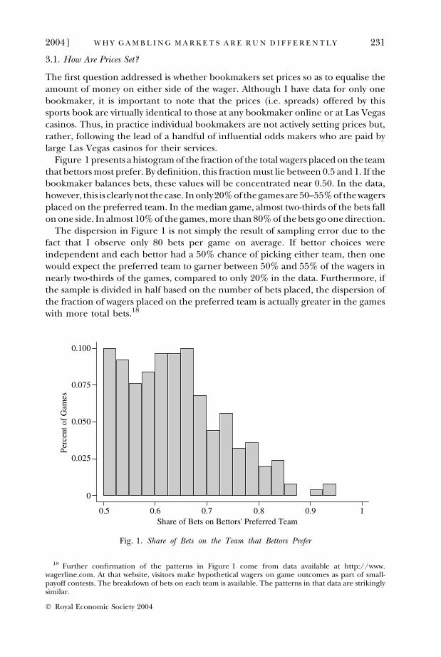
Figure 1 presents a histogram of the fraction of the total wagers placed on the teamthat bettors most prefer. By definition, this fraction must lie between 0.5 and 1. If thebookmaker balances bets, these values will be concentrated near 0.50. In the data,however, this is clearly not thecase. In only20% of thegamesare 50–55%of the wagersplaced on the preferred team. In the median game, almost two-thirds of the bets fallon one side. In almost 10% of the games, more than 80% of the bets go one direction.

The dispersion in Figure 1 is not simply the result of sampling error due to thefact that I observe only 80 bets per game on average. If bettor choices wereindependent and each bettor had a 50% chance of picking either team, then onewould expect the preferred team to garner between 50% and 55% of the wagers innearly two-thirds of the games, compared to only 20% in the data. Furthermore, ifthe sample is divided in half based on the number of bets placed, the dispersion ofthe fraction of wagers placed on the preferred team is actually greater in the gameswith more total bets.18

Perc

ent o

f G

ames

Share of Bets on Bettors' Preferred Team0.5 0.6 0.7 0.8 0.9 1

0

0.100

0.075

0.050

0.025

Fig. 1. Share of Bets on the Team that Bettors Prefer

18 Further confirmation of the patterns in Figure 1 come from data available at http://www.wagerline.com. At that website, visitors make hypothetical wagers on game outcomes as part of small-payoff contests. The breakdown of bets on each team is available. The patterns in that data are strikinglysimilar.



Two alternative hypotheses could explain the failure of the bookmaker toequalise wagers on the two sides of the spread. The first possibility is that thebookmaker would like to balance the bets but is unable to do so because it isdifficult to predict accurately what team bettors will prefer. The second hypothesisis that balancing the wagers is not the objective of the bookmaker. Indeed, asdemonstrated earlier, if bettors exhibit systematic biases, a profit maximisingbookmaker does not want to equalise the money bet on both sides. Rather, thebookmaker intentionally skews the odds such that the preferred team attractsmore wagers but wins less than half of the time.

If bookmakers are attempting to balance the money bet on each side of thewager, one would expect that observable characteristics of a team or game wouldhave no power in predicting the fraction of bettors preferring that team. Other-wise, the bookmaker could have used that information to set a spread that wouldhave better equalised the distribution of bets. If the bookmaker is attempting toexploit bettor biases by setting skewed odds, however, the opposite is true.Dimensions along which bettors exhibit bias should be systematically positivelyrelated to bet shares (and as demonstrated below, will also be systematicallynegatively related to win percentages).

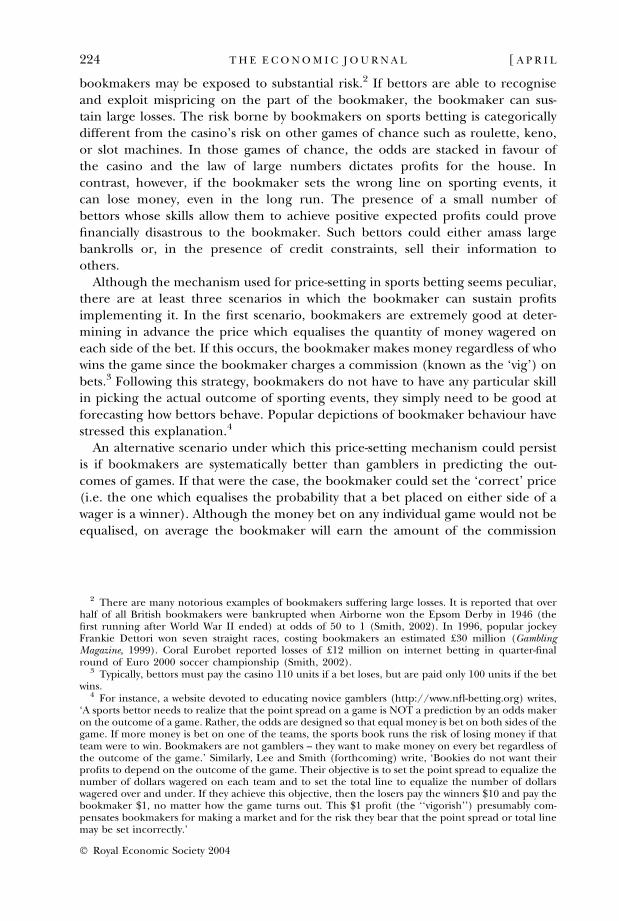
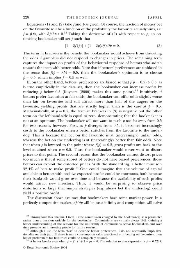
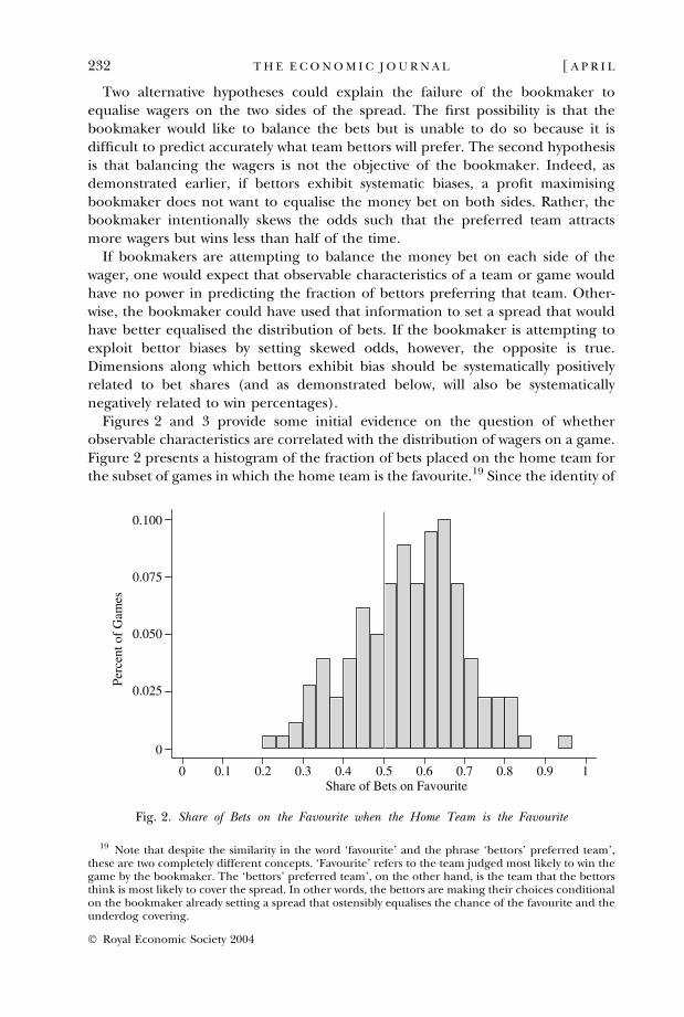
Figures 2 and 3 provide some initial evidence on the question of whetherobservable characteristics are correlated with the distribution of wagers on a game.Figure 2 presents a histogram of the fraction of bets placed on the home team forthe subset of games in which the home team is the favourite.19 Since the identity of

Perc

ent o

f G

ames

Share of Bets on Favourite0 0.1 0.2 0.3 0.4 0.5 0.6 0.7 0.8 0.9 1

0

0.100

0.075

0.050

0.025

Fig. 2. Share of Bets on the Favourite when the Home Team is the Favourite

19 Note that despite the similarity in the word ‘favourite’ and the phrase ‘bettors’ preferred team’,these are two completely different concepts. ‘Favourite’ refers to the team judged most likely to win thegame by the bookmaker. The ‘bettors’ preferred team’, on the other hand, is the team that the bettorsthink is most likely to cover the spread. In other words, the bettors are making their choices conditionalon the bookmaker already setting a spread that ostensibly equalises the chance of the favourite and theunderdog covering.



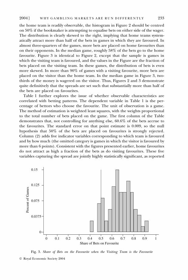
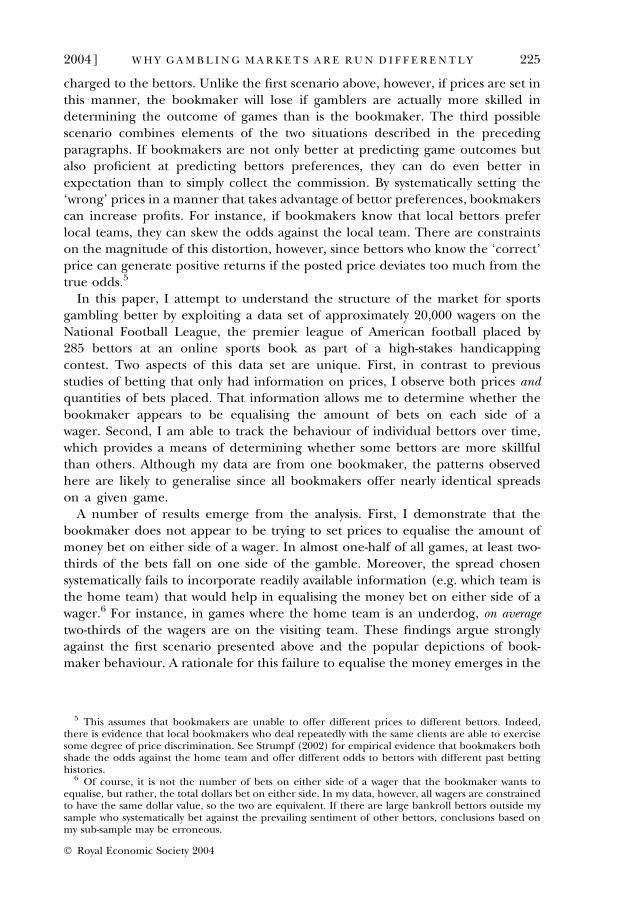
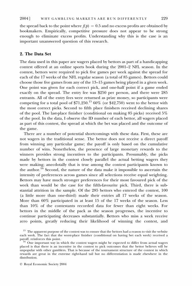
the home team is readily observable, the histogram in Figure 2 should be centredon 50% if the bookmaker is attempting to equalise bets on either side of the wager.The distribution is clearly skewed to the right, implying that home teams system-atically attract more than half of the bets in games in which they are favoured. Inalmost three-quarters of the games, more bets are placed on home favourites thanon their opponents. In the median game, roughly 58% of the bets go to the homefavourite. Figure 3 is identical to Figure 2, except that the sample is games inwhich the visiting team is favoured, and the values in the Figure are the fraction ofbets placed on the visiting team. In these games, the distribution of bets is evenmore skewed. In more than 90% of games with a visiting favourite, more bets areplaced on the visitor than the home team. In the median game in Figure 3, two-thirds of the money is wagered on the visitor. Thus, Figures 2 and 3 demonstratequite definitively that the spreads are set such that substantially more than half ofthe bets are placed on favourites.

Table 1 further explores the issue of whether observable characteristics arecorrelated with betting patterns. The dependent variable in Table 1 is the per-centage of bettors who choose the favourite. The unit of observation is a game.The method of estimation is weighted least squares, with the weights proportionalto the total number of bets placed on the game. The first column of the Tabledemonstrates that, not controlling for anything else, 60.6% of the bets accrue tothe favourites. The standard error on that point estimate is 0.009, so the nullhypothesis that 50% of the bets are placed on favourites is strongly rejected.Column (2) adds five indicator variables corresponding to which team is favouredand by how much (the omitted category is games in which the visitor is favoured bymore than 6 points). Consistent with the figures presented earlier, home favouritesdo not attract as high a fraction of the bets as do visiting favourites. These fivevariables capturing the spread are jointly highly statistically significant, as reported

Perc

ent o

f G

ames

Share of Bets on Favourite0 0.1 0.2 0.3 0.4 0.5 0.6 0.7 0.8 0.9 1

0

0.15

0.125

0.075

0.0375

Fig. 3. Share of Bets on the Favourite when the Visiting Team is the Favourite



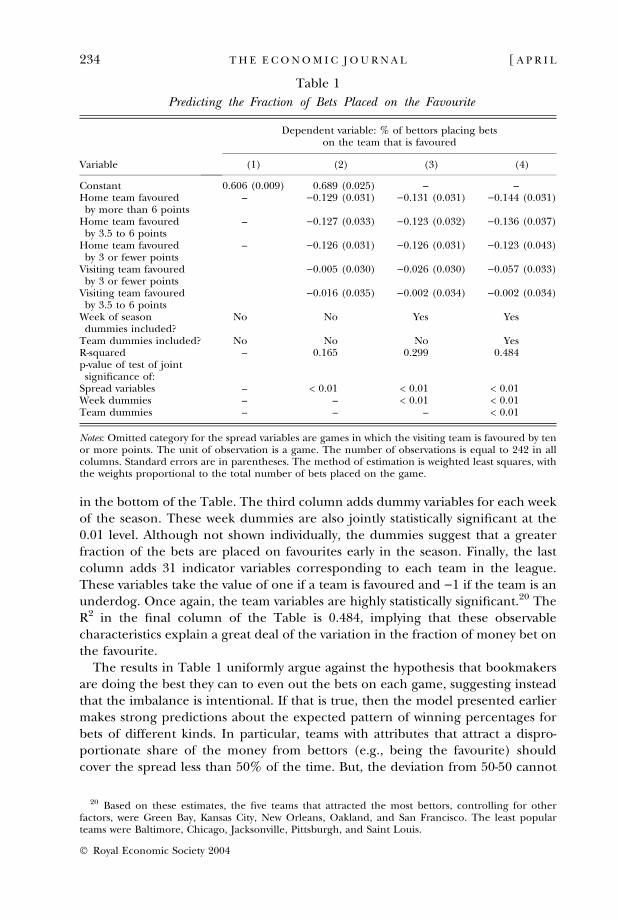
in the bottom of the Table. The third column adds dummy variables for each weekof the season. These week dummies are also jointly statistically significant at the0.01 level. Although not shown individually, the dummies suggest that a greaterfraction of the bets are placed on favourites early in the season. Finally, the lastcolumn adds 31 indicator variables corresponding to each team in the league.These variables take the value of one if a team is favoured and )1 if the team is anunderdog. Once again, the team variables are highly statistically significant.20 TheR2 in the final column of the Table is 0.484, implying that these observablecharacteristics explain a great deal of the variation in the fraction of money bet onthe favourite.

The results in Table 1 uniformly argue against the hypothesis that bookmakersare doing the best they can to even out the bets on each game, suggesting insteadthat the imbalance is intentional. If that is true, then the model presented earliermakes strong predictions about the expected pattern of winning percentages forbets of different kinds. In particular, teams with attributes that attract a dispro-portionate share of the money from bettors (e.g., being the favourite) shouldcover the spread less than 50% of the time. But, the deviation from 50-50 cannot

Table 1

Predicting the Fraction of Bets Placed on the Favourite

Variable

Dependent variable: % of bettors placing betson the team that is favoured

(1) (2) (3) (4)

Constant 0.606 (0.009) 0.689 (0.025) – –Home team favouredby more than 6 points

– )0.129 (0.031) )0.131 (0.031) )0.144 (0.031)

Home team favouredby 3.5 to 6 points

– )0.127 (0.033) )0.123 (0.032) )0.136 (0.037)

Home team favouredby 3 or fewer points

– )0.126 (0.031) )0.126 (0.031) )0.123 (0.043)

Visiting team favouredby 3 or fewer points

)0.005 (0.030) )0.026 (0.030) )0.057 (0.033)

Visiting team favouredby 3.5 to 6 points

)0.016 (0.035) )0.002 (0.034) )0.002 (0.034)

Week of seasondummies included?

No No Yes Yes

Team dummies included? No No No YesR-squared – 0.165 0.299 0.484p-value of test of jointsignificance of:

Spread variables – < 0.01 < 0.01 < 0.01Week dummies – – < 0.01 < 0.01Team dummies – – – < 0.01

Notes: Omitted category for the spread variables are games in which the visiting team is favoured by tenor more points. The unit of observation is a game. The number of observations is equal to 242 in allcolumns. Standard errors are in parentheses. The method of estimation is weighted least squares, withthe weights proportional to the total number of bets placed on the game.

20 Based on these estimates, the five teams that attracted the most bettors, controlling for otherfactors, were Green Bay, Kansas City, New Orleans, Oakland, and San Francisco. The least popularteams were Baltimore, Chicago, Jacksonville, Pittsburgh, and Saint Louis.



be too large (more than a few percentage points), or bettors who do not sufferfrom biases can profitably exploit the price distortion.

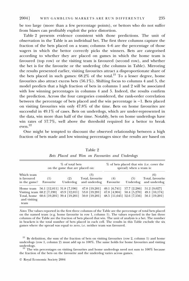
Table 2 presents evidence consistent with those predictions. The unit ofobservation in the Table is an individual bet. The first three columns capture thefraction of the bets placed on a team; columns 4–6 are the percentage of thosewagers in which the bettor correctly picks the winners. Bets are categorisedaccording to whether they are placed on games in which the home team isfavoured (top row) or the visiting team is favoured (second row), and whetherthe bet is for the favourite or the underdog (the columns in Table). Mirroringthe results presented earlier, visiting favourites attract a disproportionate share ofthe bets placed in such games: 68.2% of the total.21 To a lesser degree, homefavourites also attract excess bets (56.1%). Shifting focus to columns 4 and 5, themodel predicts that a high fraction of bets in columns 1 and 2 will be associatedwith low winning percentages in columns 4 and 5. Indeed, the results confirmthe prediction. Across the four categories considered, the rank-order correlationbetween the percentage of bets placed and the win percentage is )1. Bets placedon visiting favourites win only 47.8% of the time. Bets on home favourites aresuccessful in 49.1% of cases. Bets on underdogs, which are under-represented inthe data, win more than half of the time. Notably, bets on home underdogs havewin rates of 57.7%, well above the threshold required for a bettor to breakeven.22

One might be tempted to discount the observed relationship between a highfraction of bets made and low winning percentages since the results are based on

Table 2

Bets Placed and Won on Favourites and Underdogs

Which teamis favouredin the game?

% of total betson the game that are placed on:

% of bets placed that win (i.e. cover thespread) when a team is:

(3) (6)(1)

Favourite(2)

UnderdogTotal, favouriteand underdog

(4)Favourite

(5)Underdog

Total, favouriteand underdog

Home team 56.1 [12,011] 31.8 [7,190] 47.0 [19,201] 49.1 [6,741] 57.7 [2,286] 51.2 [9,027]Visiting team 68.2 [7,190] 43.9 [12,011] 53.0 [19,201] 47.8 [4,904] 50.4 [5,270] 49.1 [10,174]Total, homeand visitingteam

60.6 [19,201] 39.4 [19,201] 50.0 [19,201] 48.5 [11,645] 52.6 [7,556] 50.1 [19,201]

Notes: The values reported in the first three columns of the Table are the percentage of total bets placedon the named team (e.g. home favourite in row 1, column 1). The values reported in the last threecolumns of the Table are the fraction of bets placed that win. The unit of analysis is a bet. The numberin brackets is the total number of bets placed in each cell. The results in this Table exclude the sixgames where the spread was equal to zero, i.e. neither team was favoured.

21 By definition, the sum of the fraction of bets on visiting favourites (row 2, column 1) and homeunderdogs (row 1, column 2) must add up to 100%. The same holds for home favourites and visitingunderdogs.

22 The win percentages on visiting favourites and home underdogs need not sum to 100% becausethe fraction of the bets on the favourite and the underdog varies across games.



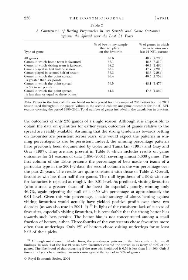
the outcomes of only 236 games of a single season. Although it is impossible toobtain the data on quantities for earlier years, outcomes of games relative to thespread are readily available. Assuming that the strong tendencies towards bettingon favourites are persistent across years, one would expect the patterns in win-ning percentages to also be persistent. Indeed, the winning percentage patternshave previously been documented by Golec and Tamarkin (1991) and Gray andGray (1997). They are also present in Table 3, which includes results on gameoutcomes for 21 seasons of data (1980–2001), covering almost 5,000 games. Thefirst column of the Table presents the percentage of bets made on teams of aparticular type in the 2001–2 data; the second column is the win percentage overthe past 21 years. The results are quite consistent with those of Table 2. Overall,favourites win less than half their games. The null hypothesis of a 50% win ratefor favourites is rejected at roughly the 0.01 level. As predicted, visiting favourites(who attract a greater share of the bets) do especially poorly, winning only46.7%, again rejecting the null of a 0.50 win percentage at approximately the0.01 level. Given this win percentage, a naive strategy of always betting againstvisiting favourites would actually have yielded positive profits over these twodecades (as was also true in 2001–2).23 In light of the consistent lack of success offavourites, especially visiting favourites, it is remarkable that the strong bettor biastowards such bets persists. The bettor bias is not concentrated among a smallfraction of bettors, either. Three-fourths of the contestants chose favourites moreoften than underdogs. Only 2% of bettors chose visiting underdogs for at leasthalf of their picks.

Table 3

A Comparison of Betting Frequencies in my Sample and Game Outcomesagainst the Spread over the Last 21 Years

Type of game

% of bets in my samplethat are placedon the favourite

% of games in whichfavourite wins over

last 21 NFL seasons

All games 60.6 48.2 [4,793]Games in which home team is favoured 56.1 48.8 [3,310]Games in which visiting team is favoured 68.2 46.7 [1,483]Games played in first half of season 63.4 47.7 [2,209]Games played in second half of season 56.3 48.5 [2,584]Games in which the point spreadis greater than six points

60.4 48.5 [1,759]

Games in which the point spreadis 3.5 to six points

59.5 48.1 [1,475]

Games in which the point spreadis less than or equal to three points

61.5 47.8 [1,559]

Notes: Values in the first column are based on bets placed for the sample of 285 bettors for the 2001season used throughout the paper. Values in the second column are game outcomes for the 21 NFLseasons covering the period 1980–2001. Total number of games included in the calculation in brackets.

23 Although not shown in tabular form, the year-by-year patterns in the data confirm the overallfindings. In only 4 of the last 21 years have favourites covered the spread in as many of 50% of thegames. The likelihood of that occurring if the true win likelihood is 0.50 is less than 1 in 300. Only 3times in 21 years have visiting favourites won against the spread in 50% of games.



Similar results are also obtained from betting on other American sporting lea-gues. Home underdogs covered the spread in 53.2% of the National CollegiateAthletic Association (NCAA) college football games played in 2002, as well as53.0% of professional basketball games in the 2002 season of the NationalBasketball Association (NBA).

Just how much do bookmakers increase their profits by exploiting bettor biasesin professional football? Assuming that (1) the total distribution of bets in thissample is representative of overall betting and (2) there is no information inaggregate bettor preferences (the evidence presented below cannot reject this), itis straightforward using the values in Table 2 to calculate that the way spreads arecurrently set, bettors should win 49.45% of their bets.24 Given the standard ‘vig’ ofbettors risking 110 units to win 100, a bookmaker who wins half his bets has a grossprofit rate of 5.0%. If bettors win only 49.45% of their bets, the expected grossprofit rate jumps to 6.16% (0.5055 · 110 ) 0.4945 · 100). Thus, in expectation,this seemingly minor distortion of the win rate increases gross profits by 23%. It istrue, of course, that the bookmaker must bear some risk when the bets are notbalanced on both sides of the wager. Because game outcomes are likely to beindependent, however, the risk is minimised as the number of games playedincreases. For instance, in the case where 63% of the money is one side of eachwager and that team wins 48% of the time, over the course of the NFL season(roughly 250 games) the bookmaker’s expected gross profit rate is 6.1% with astandard deviation of 2.5%. Thus, the bookmaker would be expected to makenegative gross profits less than once every one hundred seasons. If one looks over afive-year time frame, the standard deviation drops to 1.1%. So the probability of abookmaker losing over any given five-year period in this scenario is less than one in10,000. Relative to a 23% increase in gross profit, the costs associated with bearingthis level of risk appear minimal.25 One cost to bookmakers of bearing risk,however, is the need to have substantial liquid capital available to them in case ofan adverse shock.

The last two panels of Table 3 explore the relationship between other factorsand betting on favourites. In the 2001–2 data, a higher fraction of bets wereplaced on favourites in the first half of the season than in the second half(63.4% versus 56.3%), and the week of the season was highly statistically sig-nificant in predicting bet shares in Table 1. Whether this is simply an idio-syncracy of the 2001–2 season is uncertain. Consistent with the theory, the winpercentages for favourites over 20 years are higher in the second half of theseason (48.5 versus 47.7), although the differences is not statistically significant.Finally, the bottom panel of the Table demonstrates that the size of the spreadhas little impact on the distribution of bets on the favourite; correspondingly,

24 The number 49.45 is obtained by multiplying the probability that the home favourite wins a gametimes the percentage of total bets on home favourites plus the probability that the visiting underdogwins times the percentage of overall bets on visiting underdogs etc.

25 A major puzzle in this industry is the rarity of price competition, i.e. the vig is almost universally10%. It is possible that the bearing of risk somehow supports this equilibrium. One website, http://www.tradesports.com, acts as a traditional financial market-maker, matching buyers and sellers buttaking no positions on game outcomes. The commission charged for this match-making service is lessthan 1% of the bet – far smaller than the traditional vig.



there is little apparent difference in win percentages across these games incolumn 2.

3.2. Is There Evidence that Some Bettors Are Especially Skillful in Picking Winners?

In order for the current system of price-setting (in which the bookmakers set aprice and do not adjust that price to equilibrate supply and demand) to survive,there cannot exist a sufficient number of bettors with an ability to pick winnersthat exceeds that of the bookmaker. This is particularly true when the bookmakerdistorts prices to exploit the subset of bettors with biases. In that case, a sophisti-cated bettor only needs to be slightly better than the bookmaker in determiningthe true odds to turn a profit.26 Indeed, Strumpf (2002) argues that much of theinternal structure of bookmaker organisations is designed to protect the book-maker against adverse selection by these talented bettors.

Testing for bettor skill is complicated in my data set by the fact that there is agreat deal of attrition over the course of the sample, and the attrition is notrandom. Bettors who have performed poorly up to that point in time are muchmore likely to leave the sample since the chances of receiving a prize are very lowfor these contestants.

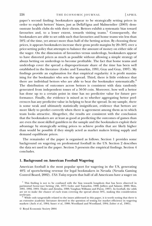
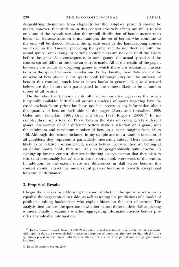
I consider two possible approaches for testing for heterogeneity in skill acrossbettors. The first approach is to look at the overall distribution of games won overthe course of the season and to test whether that distribution is consistent with thatwhich would have been generated by homogeneous bettors.27 Because of attrition,however, these data are incomplete. Approximately 82% of possible bets wereactually placed. Under the assumption that the outcomes of bets on the missinggames can be modelled as being generated by independent coin tosses withprobability 0.5, it is possible to simulate what the distribution of wins would havebeen without attrition. This approach has the obvious drawback that the simulatedportion of the data is generated by the process that I have defined as the nullhypothesis against which to test. Thus, such a test is biased against rejecting thenull of no heterogeneity.28 Figure 4 presents a representative histogram of thedistribution of these simulated final win totals. Superimposed on the histogram isthe corresponding normal distribution which the data would be expected toapproximate if generated by i.i.d. coin tosses with a win probability of 0.50. Visu-ally, the observed distribution closely mirrors the normal distribution. p-values forthe three generally applied tests of normality (skew test, Shapiro-Francis, andShapiro-Wilk) are well within the acceptable range. Thus, with the caveat that thetest is biased against rejection due to the simulated data, there is no evidence toreject the null hypothesis of no differences in skill across bettors in the sample.

26 And, as demonstrated above, even a naive strategy of betting against all visiting favourites has beenmarginally profitable.

27 Because the worst-place finisher gets a payoff, those near the bottom have an incentive to try topick losers intentionally. If they have some ability to do this, that will exaggerate the bottom tail,exacerbating deviations from normality.

28 In defence of the manner in which the missing data are generated, other results presented belowsuggest that there is no evidence of serial correlation across weeks in a given bettors ability to pickwinners.



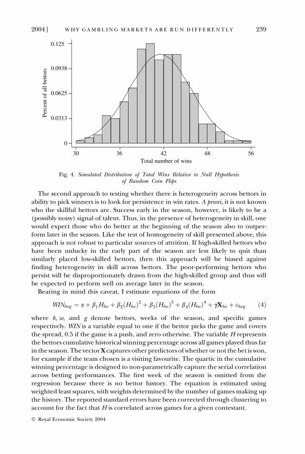
The second approach to testing whether there is heterogeneity across bettors inability to pick winners is to look for persistence in win rates. A priori, it is not knownwho the skillful bettors are. Success early in the season, however, is likely to be a(possibly noisy) signal of talent. Thus, in the presence of heterogeneity in skill, onewould expect those who do better at the beginning of the season also to outper-form later in the season. Like the test of homogeneity of skill presented above, thisapproach is not robust to particular sources of attrition. If high-skilled bettors whohave been unlucky in the early part of the season are less likely to quit thansimilarly placed low-skilled bettors, then this approach will be biased againstfinding heterogeneity in skill across bettors. The poor-performing bettors whopersist will be disproportionately drawn from the high-skilled group and thus willbe expected to perform well on average later in the season.

Bearing in mind this caveat, I estimate equations of the form

WINbwg ¼ a þ b1Hbw þ b2ðHbwÞ2 þ b3ðHbwÞ3 þ b4ðHbwÞ4 þ cXbw þ ebwg ð4Þ

where b, w, and g denote bettors, weeks of the season, and specific gamesrespectively. WIN is a variable equal to one if the bettor picks the game and coversthe spread, 0.5 if the game is a push, and zero otherwise. The variable H representsthe bettors cumulative historical winning percentage across all games played thus farin the season. The vector X captures other predictors of whether or not the bet is won,for example if the team chosen is a visiting favourite. The quartic in the cumulativewinning percentage is designed to non-parametrically capture the serial correlationacross betting performances. The first week of the season is omitted from theregression because there is no bettor history. The equation is estimated usingweighted least squares, with weights determined by the number of games making upthe history. The reported standard errors have been corrected through clustering toaccount for the fact that H is correlated across games for a given contestant.

Perc

ent o

f al

l bet

tors

Total number of wins30 36 42 48 56

0

0.125

0.0938

0.0625

0.0313

Fig. 4. Simulated Distribution of Total Wins Relative to Null Hypothesisof Random Coin Flips



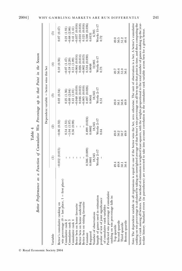
Table 4 reports results of the estimation. In the first column, the cumulativebetting success rate is constrained to enter linearly. Although not statisticallysignificant, the point estimate implies that bettors who have been more suc-cessful up until that point in the season are predicted to do slightly worse in thecurrent week. This argues against heterogeneity in skill across bettors, whichwould lead to a positive coefficient. The bottom panel of the Table reports thepredicted success rate for bettors with varying win percentages up to this pointin the season. The second equation adds the quartic in betting history. Althoughthe history variables are jointly statistically significant, the R2 is very low (0.0004).Most bettors averaging are predicted to perform right around 50%, bettors inthe top quartile prior to this week are projected to win only 49.0% of games.Once again, these results argue against persistent differences in skill. Addingcovariates in column 3 has little impact on the conclusions. Columns 4 and 5restrict the sample to exclude the first five and ten weeks respectively, on therationale that cumulative win percentages early in the season may not be veryinformative. The results provide no evidence that strong past performancepredicts wins today.

In summary, there is little in the data to suggest that, at least in this particularsample, there is heterogeneity in skill across bettors. This result may be due par-tially to the relative sophistication of bettors in the sample – perhaps the mostnaive bettors are unlikely to frequent internet bookmakers.29

3.3. Does Pooling Information Across Bettor Preferences Help in Predictingthe Outcome of Games?

In other contexts, it has been argued that aggregating information across agentsprovides valuable information in predicting future outcomes. For example, Clemenand Winkler (1986) and Fomby and Samant (1991) find that the consensus esti-mate of future GNP growth is a better predictor than any one individual’s estimate.One might also expect such a pattern to be present in sports betting, especiallybecause price is set unilaterally by the bookmaker. To the extent that the book-maker sometimes makes mistakes, one would expect that many bettors will simul-taneously recognise the presence of the mistake and disproportionately pick oneteam.

There is one simple result in my data which suggests that aggregating opinionsacross bettors may carry valuable information: despite the fact that more than halfthe money is bet on favourites and the bookmaker set the odds so that favourites winless than half the games, the overall winning percentage for bets placed is 50.1%. Asnoted earlier, based on the odds offered by the bookmaker and the distribution ofmoney bet, one would expect 49.45% of all bets to win if there was no correlationbetween the percentage of bettors choosing a game and the game’s outcome. Thedifference between 50.1% and 49.45% implies that games in which a greater frac-

29 Strumpf (2002), for instance, reports the existence of a fraction of New York bettors who always beton the Yankees, even though the bookmakers, knowing their preferences, systematically offer thesebettors substantially worse odds than other clients.



Tab

le4

Bet

tor

Per

form

ance

asa

Fun

ctio

nof

Cu

mu

lati

veW

inP

erce

nta

geu

pto

that

Poi

nt

inth

eSe

ason

Var

iab

le

Dep

end

ent

vari

able

¼b

etto

rw

ins

this

bet

(1)

(2)

(3)

(4)

(5)

Bet

tor’

scu

mu

lati

vera

nki

ng

on

win

per

cen

tage

(0¼

last

pla

ce,

1¼

firs

tp

lace

))

0.01

2(0

.015

))

0.06

(0.3

2)0.

03(0

.34)

0.10

(0.3

6)0.

07(0

.47)

Cu

mu

lati

vera

nk

2–

0.54

(1.3

1)0.

25(1

.36)

)0.

07(1

.47)

0.21

(1.9

1)C

um

ula

tive

ran

k3

–)

1.04

(1.9

7))

0.69

(2.0

4))

0.18

(2.2

0))

0.68

(2.8

6)C

um

ula

tive

ran

k4

–0.

56(0

.98)

0.41

(1.0

1)0.

15(1

.09)

0.41

(1.4

1)B

etto

rb

ets

on

ho

me

favo

uri

te–

–)

0.04

8(0

.010

))

0.06

4(0

.014

))

0.03

7(0

.016

)B

etto

rb

ets

on

ho

me

un

der

do

g–

–0.

046

(0.0

12)

0.02

6(0

.014

))

0.01

0(0

.018

)B

etto

rb

ets

on

visi

tin

gfa

vou

rite

––

)0.

005

(0.0

10)

)0.

002

(0.0

13)

0.12

1(0

.016

)C

on

stan

t0.

506

(0.0

09)

0.49

9(0

.024

)0.

497

(0.0

26)

0.53

4(0

.030

)0.

598

(0.0

36)

R-s

qu

ared

0.00

010.

0002

0.00

410.

0048

0.01

31N

um

ber

of

ob

serv

atio

ns

18,3

4518

,345

18,3

4512

,985

6,78

5Sa

mp

leo

fga

mes

use

din

esti

mat

ion

Wee

ks2–

17W

eeks

2–17

Wee

ks2–

17W

eeks

6–17

Wee

ks11

–17

p-v

alu

eo

fte

sto

fjo

int

sign

ifica

nce

of

cum

ula

tive

ran

kva

riab

les

–0.

640.

510.

730.

72

Pre

dic

ted

win

per

cen

tage

ifcu

mu

lati

vera

nki

ng

on

win

per

cen

tage

fall

sin

:T

op

qu

arti

le49

.449

.049

.049

.749

.0Se

con

dq

uar

tile

49.8

50.2

50.1

50.4

50.5

Th

ird

qu

arti

le50

.150

.750

.851

.051

.2B

ott

om

qu

arti

le50

.449

.949

.950

.149

.4

Not

es:

Th

ed

epen

den

tva

riab

lein

all

regr

essi

on

sis

equ

alto

on

eif

the

bet

tor

win

sth

eb

et,

zero

oth

erw

ise.

Th

eu

nit

of

ob

serv

atio

nis

ab

et.

Ab

etto

r’s

cum

ula

tive

ran

kin

go

nw

inp

erce

nta

geis

calc

ula

ted

by

taki

ng

anu

nw

eigh

ted

aver

age

of

that

bet

tor’

sw

inp

erce

nta

geo

nal

lbet

su

pto

that

po

int

inti

me,

and

then

com

pu

tin

gth

eb

etto

r’s

ran

kam

on

gal

lb

etto

rs.T

he

met

ho

do

fes

tim

atio

nis

wei

ghte

dle

ast

squ

ares

,wit

hth

ew

eigh

tsp

rop

ort

ion

alto

the

tota

ln

um

ber

of

gam

esm

akin

gu

pth

eye

ar-

to-d

ate

his

tory

.St

and

ard

erro

rs(i

np

aren

thes

es)

are

corr

ecte

dto

take

into

acco

un

tco

rrel

atio

nin

the

cum

ula

tive

ran

kva

riab

leac

ross

bet

sfo

ra

give

nb

etto

r.



tion of bettors choose the favourite (or alternatively the underdog) are more likelyto be won by the favourite (underdog). Thus, in principle one might believe thatknowledge of aggregate bettor preferences might be useful in prediction, makingaccess to quantity data (which is in general very difficult to obtain, but is availableprior to the start of the games through this contest) valuable.30

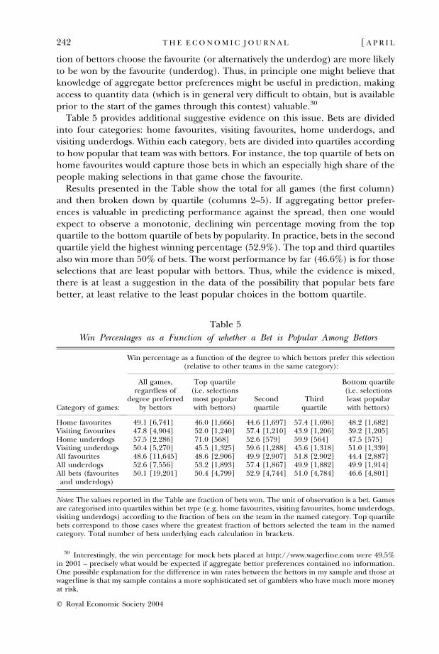
Table 5 provides additional suggestive evidence on this issue. Bets are dividedinto four categories: home favourites, visiting favourites, home underdogs, andvisiting underdogs. Within each category, bets are divided into quartiles accordingto how popular that team was with bettors. For instance, the top quartile of bets onhome favourites would capture those bets in which an especially high share of thepeople making selections in that game chose the favourite.

Results presented in the Table show the total for all games (the first column)and then broken down by quartile (columns 2–5). If aggregating bettor prefer-ences is valuable in predicting performance against the spread, then one wouldexpect to observe a monotonic, declining win percentage moving from the topquartile to the bottom quartile of bets by popularity. In practice, bets in the secondquartile yield the highest winning percentage (52.9%). The top and third quartilesalso win more than 50% of bets. The worst performance by far (46.6%) is for thoseselections that are least popular with bettors. Thus, while the evidence is mixed,there is at least a suggestion in the data of the possibility that popular bets farebetter, at least relative to the least popular choices in the bottom quartile.

Table 5

Win Percentages as a Function of whether a Bet is Popular Among Bettors

Category of games:

Win percentage as a function of the degree to which bettors prefer this selection(relative to other teams in the same category):

All games,regardless of

degree preferredby bettors

Top quartile(i.e. selectionsmost popularwith bettors)

Secondquartile

Thirdquartile

Bottom quartile(i.e. selectionsleast popularwith bettors)

Home favourites 49.1 [6,741] 46.0 [1,666] 44.6 [1,697] 57.4 [1,696] 48.2 [1,682]Visiting favourites 47.8 [4,904] 52.0 [1,240] 57.4 [1,210] 43.9 [1,206] 39.2 [1,205]Home underdogs 57.5 [2,286] 71.0 [568] 52.6 [579] 59.9 [564] 47.5 [575]Visiting underdogs 50.4 [5,270] 45.5 [1,325] 59.6 [1,288] 45.6 [1,318] 51.0 [1,339]All favourites 48.6 [11,645] 48.6 [2,906] 49.9 [2,907] 51.8 [2,902] 44.4 [2,887]All underdogs 52.6 [7,556] 53.2 [1,893] 57.4 [1,867] 49.9 [1,882] 49.9 [1,914]All bets (favouritesand underdogs)

50.1 [19,201] 50.4 [4,799] 52.9 [4,744] 51.0 [4,784] 46.6 [4,801]

Notes: The values reported in the Table are fraction of bets won. The unit of observation is a bet. Gamesare categorised into quartiles within bet type (e.g. home favourites, visiting favourites, home underdogs,visiting underdogs) according to the fraction of bets on the team in the named category. Top quartilebets correspond to those cases where the greatest fraction of bettors selected the team in the namedcategory. Total number of bets underlying each calculation in brackets.

30 Interestingly, the win percentage for mock bets placed at http://www.wagerline.com were 49.5%in 2001 – precisely what would be expected if aggregate bettor preferences contained no information.One possible explanation for the difference in win rates between the bettors in my sample and those atwagerline is that my sample contains a more sophisticated set of gamblers who have much more moneyat risk.



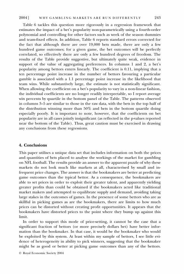
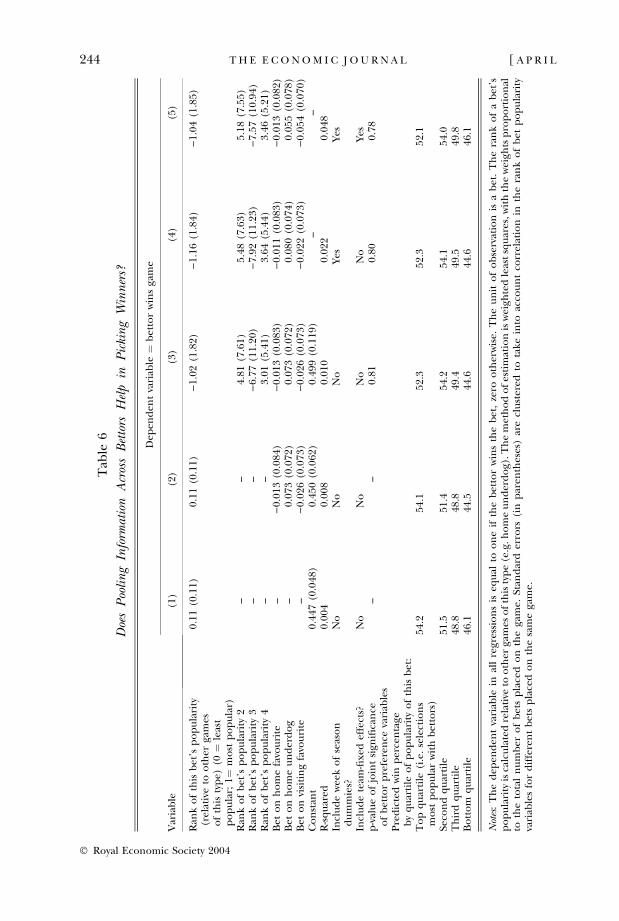
Table 6 tackles this question more rigorously in a regression framework thatestimates the impact of a bet’s popularity non-parametrically using a fourth-orderpolynomial and controlling for other factors such as week of the season dummiesand team-fixed effects. In addition, Table 6 reports standard errors corrected forthe fact that although there are over 19,000 bets made, there are only a fewhundred game outcomes; for a given game, the bet outcomes will be perfectlycorrelated, so effectively there are only a few hundred degrees of freedom. Theresults of the Table provide suggestive, but ultimately quite weak, evidence insupport of the value of aggregating preferences. In columns 1 and 2, a bet’spopularity among bettors enters linearly. The coefficient is 0.11, implying that aten percentage point increase in the number of bettors favouring a particulargamble is associated with a 1.1 percentage point increase in the likelihood thatteam wins. While substantively large, the estimate is not statistically significant.When allowing the coefficient on a bet’s popularity to vary in a non-linear fashion,the individual coefficients are no longer readily interpretable, so I report averagewin percents by quartile in the bottom panel of the Table. The patterns observedin columns 3–5 are similar to those in the raw data, with the bets in the top half ofthe distribution winning more than 50% and bets in the bottom quartile doingespecially poorly. It is important to note, however, that the coefficients on betpopularity are in all cases jointly insignificant (as reflected in the p-values reportednear the bottom of the Table). Thus, great caution must be exercised in drawingany conclusions from these regressions.

4. Conclusions

This paper utilises a unique data set that includes information on both the pricesand quantities of bets placed to analyse the workings of the market for gamblingon NFL football. The results provide an answer to the apparent puzzle of why thesemarkets do not look much like markets at all, characterised by small and in-frequent price changes. The answer is that the bookmakers are better at predictinggame outcomes than the typical bettor. As a consequence, the bookmakers areable to set prices in order to exploit their greater talent, and apparently yieldinggreater profits than could be obtained if the bookmakers acted like traditionalmarket makers and attempted to equilibrate supply and demand, avoiding takinglarge stakes in the outcomes of games. In the presence of some bettors who are asskillful in picking games as are the bookmakers, there are limits to how muchprices can be distorted without creating profit opportunities. It appears that thebookmakers have distorted prices to the point where they bump up against thislimit.

In order to support this mode of price-setting, it cannot be the case that asignificant fraction of bettors (or more precisely dollars bet) have better infor-mation than the bookmaker. In that case, it would be the bookmaker who wouldbe exploited by this system. At least within my sample of bettors, I see little evi-dence of heterogeneity in ability to pick winners, suggesting that the bookmakermight be as good or better at picking game outcomes than any of the bettors.



Tab

le6

Doe

sP

ooli

ng

Info

rmat

ion

Acr

oss

Bet

tors

Hel

pin

Pic

kin

gW

inn

ers?

Var

iab

le

Dep

end

ent

vari

able

¼b

etto

rw

ins

gam

e

(1)

(2)

(3)

(4)

(5)

Ran

ko

fth

isb

et’s

po

pu

lari

ty(r

elat

ive

too

ther

gam

eso

fth

isty

pe)

(0¼

leas

tp

op

ula

r;1¼

mo

stp

op

ula

r)

0.11

(0.1

1)0.

11(0

.11)

)1.

02(1

.82)

)1.

16(1

.84)

)1.

04(1

.85)

Ran

ko

fb

et’s

po

pu

lari

ty2

––

4.81

(7.6

1)5.

48(7

.63)

5.18

(7.5

5)R

ank

of

bet

’sp

op

ula

rity

3–

–)

6.77

(11.

20)

)7.

92(1

1.23

))

7.57

(10.

94)

Ran

ko

fb

et’s

po

pu

lari

ty4

––

3.01

(5.4

1)3.

64(5

.44)

3.46

(5.2

1)B

eto

nh

om

efa

vou

rite

–)

0.01

3(0

.084

))

0.01

3(0

.083

))

0.01

1(0

.083

))

0.01

3(0

.082

)B

eto

nh

om

eu

nd

erd

og

–0.

073

(0.0

72)

0.07

3(0

.072

)0.

080

(0.0

74)

0.05

5(0

.078

)B

eto

nvi

siti

ng

favo

uri

te–

)0.

026

(0.0

73)

)0.

026

(0.0

73)

)0.

022

(0.0

73)

)0.

054

(0.0

70)

Co

nst

ant

0.44

7(0

.048

)0.

450

(0.0

62)

0.49

9(0

.119

)–

–R

-sq

uar

ed0.

004

0.00

80.

010

0.02

20.

048

Incl

ud

ew

eek

of

seas

on

du

mm

ies?

No

No

No

Yes

Yes

Incl

ud

ete

am-fi

xed

effe

cts?

No

No

No

No

Yes

p-v

alu

eo

fjo

int

sign

ifica

nce

of

bet

tor

pre

fere

nce

vari

able

s–

–0.

810.

800.

78

Pre

dic

ted

win

per

cen

tage

by

qu

arti

leo

fp

op

ula

rity

of

this

bet

:T

op

qu

arti

le(i

.e.

sele

ctio

ns

mo

stp

op

ula

rw

ith

bet

tors

)54

.254

.152

.352

.352

.1

Seco

nd

qu

arti

le51

.551

.454

.254

.154

.0T

hir

dq

uar

tile

48.8

48.8

49.4

49.5

49.8

Bo

tto

mq

uar

tile

46.1

44.5

44.6

44.6

46.1

Not

es:

Th

ed

epen

den

tva

riab

lein

all

regr

essi

on

sis

equ

alto

on

eif

the

bet

tor

win

sth

eb

et,

zero

oth

erw

ise.

Th

eu

nit

of

ob

serv

atio

nis

ab

et.

Th

era

nk

of

ab

et’s

po

pu

lari

tyis

calc

ula

ted

rela

tive

too

ther

gam

eso

fth

isty

pe

(e.g

.ho

me

un

der

do

g).T

he

met

ho

do

fes

tim

atio

nis

wei

ghte

dle

ast

squ

ares

,wit

hth

ew

eigh

tsp

rop

ort

ion

alto

the

tota

ln

um

ber

of

bet

sp

lace

do

nth

ega

me.

Stan

dar

der

rors

(in

par

enth

eses

)ar

ecl

ust

ered

tota

kein

toac

cou

nt

corr

elat

ion

inth

era

nk

of

bet

po

pu

lari

tyva

riab

les

for

dif

fere

nt

bet

sp

lace

do

nth

esa

me

gam

e.



Given the incentives for the bookmaker to get the spread right, it is hardly sur-prising that the most talented individuals would be employed as the odds makers.

Perhaps, then, a fundamental difference between gambling and financial mar-kets is that it is possible in gambling to find and hire a small set of individuals (theodds makers) who can systematically do better in predicting game outcomes thancan bettors overall. In financial markets, on the other hand, the flow of insideinformation or the inherent complexity in valuing companies may make itimpossible for one individual to do better than the market, meaning that a marketmaker who acted like a bookmaker would do worse than one who simply equili-brated supply and demand and took advantage of the bid-ask spread. The weightof the evidence regarding the inability of fund managers to systematically beat themarket indexes is consistent with this conjecture.

University of Chicago and American Bar Foundation

References

Ali, M. (1977). ‘Probability and utility estimates for racetrack bettors’, Journal of Political Economy, vol. 85,(August), pp. 803–15.

Asch, P., Malkiel, B. and Quandt, R. (1984). ‘Market efficiency in racetrack betting’, Journal of Business,vol. 57, pp. 165–75.

Avery, C. and Chevalier, J. (1999). ‘Identifying investor sentiment from price paths: the case of footballbetting’, Journal of Business, vol. 72, (October), pp. 493–21.

Clemen, R. and Winkler, R. (1986). ‘Combining economic forecasts’, Journal of Business and EconomicStatistics, vol. 4, (January), pp. 369–91.

DellaVigna, S. and Malmendier, U. (2003). ‘Contract design and self-control: theory and evidence’,unpublished manuscript, University of California-Berkeley Department of Economics.

Fomby, T. and Samanta, S. (1991). ‘Application of stein rules to combination forecasting’, Journal ofBusiness and Economic Statistics, vol. 9, (October), pp. 391–407.

Gambling Magazine (1999). ‘Bookies still counting the costs’, published on the internet at http://www.gamblingmagazine.com/articles/31/31-57.htm.

Golec, J. and Tamarkin, M. (1991). ‘The degree of price inefficiency in the football betting markets’,Journal of Financial Economics, vol. 30, pp. 311–23.

Golec, J. and Tamarkin, M. (1998). ‘Bettors love skewness, not risk, at the horse track’, Journal of PoliticalEconomy, vol. 106, (February), pp. 205–25.

Gray, P. and Gray, S. (1997). ‘Testing market efficiency: evidence from the NFL sports betting market’,Journal of Finance, vol. 52, (September), pp. 1725–37.

Jullien, B. and Salanie, B. (2000). ‘Estimating preferences under risk: the case of racetrack bettors’,Journal of Political Economy, vol. 108, (June), pp. 503–30.

Kuypers, T. (2000). ‘Information and efficiency: an empirical study of a fixed odds betting market’,Applied Economics, vol. 32, pp. 1353–63.

Lee, M. and Smith, G. (forthcoming). ‘Regression to the mean and football wagers’, Journal of BehavioralDecisionmaking.

National Gambling Impact Study Commission (1999). Final Report, Washington, D.C.Nevada Gaming Control Board (2002). ‘Nevada gaming revenues calendar year 2001 analysis’, press

release, February 12.Sauer, R., Brajer, V., Ferris, S. and Marr, M. (1988). ‘Hold your bets: another look at the efficiency of the

gambling market for national football league games’, Journal of Political Economy, vol. 96, (February),pp. 206–13.

Shin, H. (1991). ‘Optimal betting odds against insider traders’, Economic Journal, vol. 101,(September), pp. 1179–85.

Shin, H. (1992). ‘Prices of state contingent claims with insider traders, and the favourite-longshot bias’,Economic Journal, vol. 102, (March), pp. 426–35.

Shin, H. (1993). ‘Measuring the incidence of insider trading in a market for state-contingent claims’,Economic Journal, vol. 103, (September), pp. 1141–53.

Smith, J. (2002). ‘Bookies who lose’, posted at http://www.betasia.com and reprinted from Business Life(March 2001).



Strumpf, K. (2002). ‘Illegal sports bookmakers’, Mimeo, University of North Carolina. Department ofEconomics.

Thaler, R. and Ziemba, W. (1988). ‘Parimutuel betting markets: racetracks and lotteries’, Journal ofEconomic Perspectives, vol. 2, pp. 161–74.

Vaughn Williams, L. and Paton, D. (1997). ‘Why is there a favourite-longshot bias in British racetrackbetting markets?’, Economic Journal, vol. 107, (January), pp. 150–8.

Woodland, B. and Woodland, L. (1991). ‘The effects of risk aversion on wagering: point spreads versusodds’, Journal of Political Economy, vol. 99, (June), pp. 638–53.

Woodland, B. and Woodland, L. (1994). ‘Market efficiency and the favourite-longshot bias: the baseballbetting market’, Journal of Finance, vol. 49, (March), pp. 269–79.

Zuber, R., Gandar, J. and Bowers, B. (1985). ‘Beating the spread: testing the efficiency of the gamblingmarket for national football league games’, Journal of Political Economy, vol. 93, (August), pp. 800–6.

246 [ A P R I L 2004]T H E E C O N O M I C J O U R N A L


why are gambling markets organised so differently …aldous/157/papers/levitt_gambling... · why...

Documents