who makes the most? measuring the “urban environmental virtuosity”

Who Makes the Most? Measuring the ‘‘UrbanEnvironmental Virtuosity’’

Oriana Romano • Salvatore Ercolano

Accepted: 30 April 2012 / Published online: 20 May 2012� Springer Science+Business Media B.V. 2012

Abstract This paper advances a composite indicator called urban environmental virtu-

osity index (UEVI), in order to measure the efforts made by public local bodies in applying

an ecosystem approach to urban management. UEVI employs the less exploited process-

based selection criteria for representing the original concept of virtuosity, providing makes

a cross cities comparison. In developing such a framework the main technical issue of

constructing a composite indicator, involving the weighting and the aggregation phases

will be overcame by using a multivariate approach.

Keywords Sustainability � Urban policies �Multivariate analysis � Composite indicators �Urban sustainability indicators

1 Introduction

Over recent years the number of indicators that synthesize the complex phenomenon of the

environment, mainly for communication and benchmarking purposes, has increased dra-

matically (Saisana and Tarantola 2002).

However, important controversial issues persist, such as: the selection criteria for their

construction (Niemeijer and de Groot 2008); the methodological problems related to the

weighting of variables and their aggregation (OECD 2008): and their usefulness for

decision making process (Saltelli 2007). Moreover, it is evident that the great bulk of

environmental indices focuses on national rather than local entities and thus fails to capture

differences between localities and eventually the changes in policies necessary to maintain

natural capital, reduce pollution and preserve biodiversity.

O. Romano (&) � S. ErcolanoDepartment of Social Sciences, University of Naples ‘‘L’Orientale’’, Largo San Giovanni Maggiore 30,80134 Naples, Italye-mail: [email protected]

S. Ercolanoe-mail: [email protected]

123

Soc Indic Res (2013) 112:709–724DOI 10.1007/s11205-012-0078-9

This paper is concerned to overcome these issues, advancing a composite indicator

called urban environmental virtuosity index (UEVI). Based on the little known process-

based knowledge approach to constructing environmental indices (Niemeijer and de Groot

2008), UEVI introduces the new concept of ‘‘virtuosity’’, in order to evaluate the efforts of

local government in tackling environmental goals. UEVI is built upon three main char-

acteristics. These are (a) a cross cities comparison; (b) a process-based selection criteria for

representing the concept of virtuosity; and (c) the employment of multivariate analysis so

to base weights on a statistical model rather than on subjective judgements.

Considerable recognition has been given to the importance of the locality in environ-

mental thinking: the UN: Rio de Janeiro Conference in 1992, Habitat Istanbul Conference

in 1996; OECD: Cities for Citizens. Improving Metropolitan Governance, 2000 and

European Union Aalborg Charter, 1994, to provide some examples, all promote strongly an

urban sustainability approach.

Following the sustainability principle, policies and actions implemented at local level

should aim to promote economic growth while providing essential services, without

compromising the natural environment. The objective of urban environmental sustain-

ability can be traced back to the 1994 ‘‘Charter of European Cities and Towns towards

Sustainability’’ (Aalborg Chart), requiring local authorities to commit to, for example,

‘‘investments in conserving the remaining natural capital, such as groundwater stocks, soil,

habitats for rare species; encouraging the use of renewable energy; investments to relieve

pressure on natural capital stocks by expanding cultivated natural capital, such as parks for

inner-city recreation to relieve pressure on natural forests; and increasing the end-use

efficiency of products, such as energy-efficient buildings, environmentally friendly urban

transport’’ (European Commission 1994, p. 2). However, discharging these strategies in it

does not necessarily mean that a city is sustainable, as several factors (i.e. population,

geographical, cultural, educational conditions, etc.) may deeply affect the performance.

Nevertheless, such actions may be regarded as being ‘‘virtuous’’ as they demonstrates the

efforts made by public local bodies in applying an ecosystem approach to urban man-

agement. The aim of this paper is to measure the urban virtuosity, by a composite indicator

using a ‘‘process oriented’’ variables framework, which provides an analytical picture of

the responses provided by local authorities to environmental problems, such as pollution

from traffic and waste, noise, unhealthy buildings, lack of green and scarce quality of water

and of the actions undertaken for improving the quality of the environment and avoid

possible negative externalities. Thus UEVI seeks at filling the gap of the lack of envi-

ronmental indicators able at performing a cross cities comparison considering the above

mentioned variables and at overcoming methodological issues in the construction of such

indices. It needs to be noticed, in fact, that the massive number of environmental indicators

(see in Bohringer 2007: environmental sustainability index (ESI), environmental perfor-

mance index (EPI), environmental vulnerability index (EVI), ecological footprint (EF);

Niemeijer 2002) developed since the 1990s (Singh et al. 2009) is related to a nation scale,

rather than a smaller one.

In developing such a framework the main technical issue is that of constructing a

composite indicator, involving the thorny problem of how to ascribe weights to the sep-

arate sub-indicators identified as being important. (Nardo et al. 2005) and then add them.

Generally weights can be equally distributed for all indicators, or assigned on the basis of

public/expert opinion. This could be not always desirable in circumstances in which a high

degree of objectivity and accuracy is required. Thus, in order to obtain weights directly

from a statistical model we will employ the principal component analysis (PCA), in which

weights are taken from the matrix of factor loadings after rotation. Moreover, as OECD

710 O. Romano, S. Ercolano

123

(2008) claims in PCA ‘‘weighting intervenes only to correct for overlapping information

between two or more correlated indicators and is not a measure of the theoretical

importance of the associated indicator’’ (OECD 2008, p. 89).

The paper is structured as follow: after presenting a background on the urban envi-

ronmental indicators literature (Sect. 2), information on data and methodology will be

provided (Sect. 3) and an empirical test on Italian capital provinces will be performed

(Sect. 4). In order to investigate those variables that may affect UEVI an OLS regression

analysis is conducted in Sect. 5. Finally, conscious of the limitations of composite indi-

cators in giving robust messages to decision makers, because of the loss of information that

occurs in the aggregation process, Sect. 6 feature a cluster analysis. It will lead at iden-

tifying specifically those variables that positively or negatively are related to the statistical

unit under observation. In Sect. 7 conclusions are drawn.

2 Background to Urban Environmental Indicators

The extensive literature on urban environmental indicators can be summarised as follows:

• The ‘‘environment’’ can be considered only as a component of a more general valuation

of the whole performance of cities and their sustainability, which include social and

economical parameters (see ‘‘city development index’’—CDI, UN 2002; urban

sustainability index (USI) Zhang 2002).1

• The broader concept of urban environment can be represented by several composite

indicators, one for each environmental aspect considered (water, waste, energy, etc. as

reported in ‘‘European Common Indicators’’, Rapporto Ambiente Italia 2003).

• Process oriented variables are used in the DPSIR (OECD 1993) model (see ‘‘Urban

Ecosystem’’ Legambiente 1994; Istat 2009 and ‘‘Index of Environmental Friendliness’’

Puolamaa et al. 1996, which is based on pressure factors). However, to date composite

indicators based uniquely on the ‘‘responses’’ to environmental problems remain

illusive.

• Indicators are focused on specific contexts rather than on cross cities comparisons.

Local indices are mainly used for assisting the local municipalities to monitor and

evaluate their environmental performance. For example the ‘‘Synthetic Environmental

Indices’’ (Isla 1996) are calculated considering the arithmetic average of 22 sub-

indicators (Saisana and Tarantola 2002) related to the environmental performance of

the city of Barcelona; while Environmental statistics of Helsinki (Helsinki City Urban

Facts Office 2002) is a report that provides a study of the impact of human activities on

the environment. Other examples related to the sustainability in the cities are:

Sustainability Index for Taipei (in Singh et al. 2009); Compass Index of Sustainability

for the city of Orlando (Atkinson et al. 1997); Sustainable Seattle: developing

Indicators of Sustainable Community (in Singh et al. 2009).

From a technical point of view the main difficulty in constructing an urban indicator is

the paucity of data: at the local level the availability of data is extremely variable, partly

owing to the fact that they are obtained not only from published statistical sources, but also

from interviews and questionnaires (OECD 1993). Moreover, local data are not always

available for all the statistical units considered (cities for example), which make the cross

1 Total urban sustainability score is based on three components of the urban sustainability in China: theurban development capacity, urban coordination capacity and urban development potential.

Who Makes the Most? 711

123

cities comparison difficult. The main technical issues relating to the arbitrary nature by

which the variables are weighted and then aggregated (Nardo et al. 2005), concern how to

scale when drawing upon local as well as national data (Saisana and Tarantola 2002).

There are several techniques employed in the weighting process and as suggested in

Saisana and Tarantola (2002, p. 52) ‘‘[…] a typical feature of some weighting procedures is

the identification of correlations in the set of indicators. A good strategy is to use several

different analytical techniques to explore groups of indicators. The analysis of correlation

patterns, through the use of some of the techniques like PCA, is indeed extremely

interesting’’.

This represents the starting point for the indicator we are going to build. The aim is to

measure ‘‘virtuosity’’ using PCA, and has crucial implications for benchmarking:2 UEVI

could be a point of reference in order to measure the environmental management ability of

the cities. This is the reason why ‘‘process oriented’’ (i.e. actions set out in sectors such as

transport, waste, water, energy, etc.) variables rather than ‘‘outcome oriented’’ (i.e. envi-

ronmental quality; urban flows; factors of pressure, etc.) will be employed. Usually the

latter are used to measure environmental sustainability strictu sensu, as they are purely

physical parameters. Thus we think that process oriented variables are more consistent with

the environmental virtuosity concept and that through them it is possible to find out the

efforts of environmental friendly policies and interventions pursued by public local

authorities in order to face up environmental problems, prevent them or ameliorate the

natural environment. Obviously, virtuosity is a necessary condition for achieving long run

sustainability.

3 Measuring Urban Environmental Virtuosity Index (UEVI): Data and Methodology

Urban environmental virtuosity can be statistically described by variables concerning

instruments and tools carried out by public subjects in order to get an environmental

friendly status. Responses to environmental problems at local level could be various and

related to several sectors. This complexity could be measured by a composite indicator,

that allow at synthesizing ‘‘multidimensional concepts which can not be captured by a

single indicator’’ (OECD 2008, p. 13).

As a result a whole picture of the efforts made by cities can be shown and a rank of the

statistical units under observation can be achievable, especially useful for benchmarking

purposes.

According with the availability of data provided by ISTAT in the (Urban Environmental

Indicators 2008),3 an empirical test will be provided. The database is the most compre-

hensive one concerning environmental issues in Italy. It covers 111 Italian capital prov-

inces, which cover the 6.6 % of Italian surface and the 29.5 % of the total population of the

Country (about 17 million of people).4

2 To be clearer, this is different from the ‘‘Environmental Policy Performance Indicator’’ (by Adriaanse A.,1993), ‘‘that indicates whether the environmental policy is heading in the right direction or not’’. It considers‘‘two independent approaches for the scaling of the theme indicators: division by the corresponding(a) sustainability levels and (b) policy targets for each theme indicator. This results in a common unit(i.e. environmental pressure equivalents—EPeq) for expressing environmental pressure within themes. Thecomposite indicator for each year is calculated as the sum of the six dimensionless theme equivalent’’(Saisana and Tarantola 2002, p. 51).3 http://www.istat.it/it/archivio/34473.4 The considered municipalities represent the main urban context in each region.


123

http://www.istat.it/it/archivio/34473

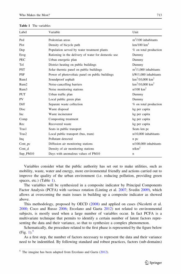
Variables consider what the public authority has set out to make utilities, such as

mobility, waste, water and energy, more environmental friendly and actions carried out to

improve the quality of the urban environment (i.e. reducing pollution, providing green

spaces, etc.) (Table 1).

The variables will be synthesized in a composite indicator by Principal Components

Factor Analysis (PCFA) with varimax rotation (Linting et al. 2007; Svedin 2009), which

allows at overcoming the main issues in building up a composite indicator as showed

above.

This methodology, proposed by OECD (2008) and applied on cases (Nicoletti et al.

2000; Coco and Russo 2006; Ercolano and Gaeta 2012) not related to environmental

subjects, is mostly used when a large number of variables occur. In fact PCFA is a

multivariate technique that permits to identify a certain number of latent factors repre-

senting the data and their variance, so that to synthesize a complex phenomenon.

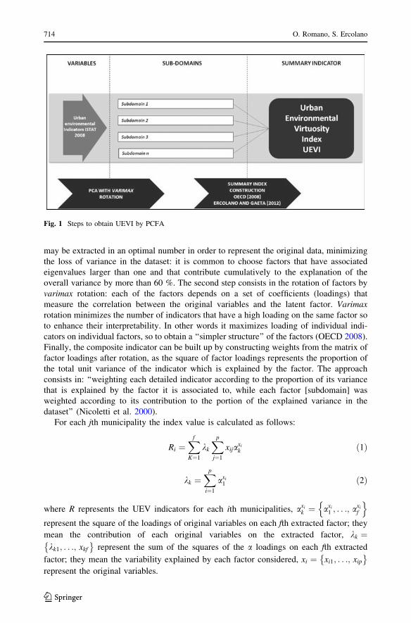
Schematically, the procedure related to the first phase is represented by the figure below

(Fig. 1).5

As a first step, the number of factors necessary to represent the data and their variance

need to be indentified. By following standard and robust practices, factors (sub-domains)

Table 1 The variables

Label Variable Unit

Ped Pedestrian areas m2/100 inhabitants

Pist Density of bicycle path km/100 km2

Dep Population served by water treatment plants % on total production

Erog Rationing in the delivery of water for domestic use Dummy

PEC Urban energetic plan Dummy

Tel District heating on public buildings Dummy

PST Solar thermic panel on public buildings m2/1,000 inhabitants

PSF Power of photovoltaic panel on public buildings kW/1,000 inhabitants

Rum1 Soundproof asphalt km2/10,000 km2

Rum2 Noise-cancelling barriers km2/10,000 km2

Rum3 Noise monitoring stations n/100 km2

PUT Urban traffic plan Dummy

PV Local public green plan Dummy

Diff Separate waste collection % on total production

Disc Waste disposal kg per capita

Inc Waste incinerator kg per capita

Comp Composting treatment kg per capita

Rec Recovered waste kg per capita

Tras1 Seats in public transport Seats km pc

Tras2 Local public transport (bus, tram) n/10,000 inhabitants

Inq Pollutant detected n pc

Cent_pc Diffusion air monitoring stations n/100,000 inhabitants

Cent_d Density of air monitoring stations n/km2

Sup_PM10 Days with anomalous values of PM10 n

5 The imagine has been adapted from Ercolano and Gaeta (2012).


123

may be extracted in an optimal number in order to represent the original data, minimizing

the loss of variance in the dataset: it is common to choose factors that have associated

eigenvalues larger than one and that contribute cumulatively to the explanation of the

overall variance by more than 60 %. The second step consists in the rotation of factors by

varimax rotation: each of the factors depends on a set of coefficients (loadings) that

measure the correlation between the original variables and the latent factor. Varimaxrotation minimizes the number of indicators that have a high loading on the same factor so

to enhance their interpretability. In other words it maximizes loading of individual indi-

cators on individual factors, so to obtain a ‘‘simpler structure’’ of the factors (OECD 2008).

Finally, the composite indicator can be built up by constructing weights from the matrix of

factor loadings after rotation, as the square of factor loadings represents the proportion of

the total unit variance of the indicator which is explained by the factor. The approach

consists in: ‘‘weighting each detailed indicator according to the proportion of its variance

that is explained by the factor it is associated to, while each factor [subdomain] was

weighted according to its contribution to the portion of the explained variance in the

dataset’’ (Nicoletti et al. 2000).

For each jth municipality the index value is calculated as follows:

Ri ¼Xf

K¼1

kk

Xp

j¼1

xijaxi

k ð1Þ

kk ¼Xp

i¼1

axi

1 ð2Þ

where R represents the UEV indicators for each ith municipalities, axi

k ¼ axi

1 ; . . .; axi

f

n o

represent the square of the loadings of original variables on each fth extracted factor; they

mean the contribution of each original variables on the extracted factor, kk ¼kk1; . . .; xkf

� �represent the sum of the squares of the a loadings on each fth extracted

factor; they mean the variability explained by each factor considered, xi ¼ xi1; . . .; xip

� �

represent the original variables.

Fig. 1 Steps to obtain UEVI by PCFA


123

4 Empirical Results

Implementing PCFA latent variables that synthesize the original selected indicators are

represented. What it should be taken into account is that each extracted factor is charac-

terized by different contributions of the original values that entirely explain the phe-

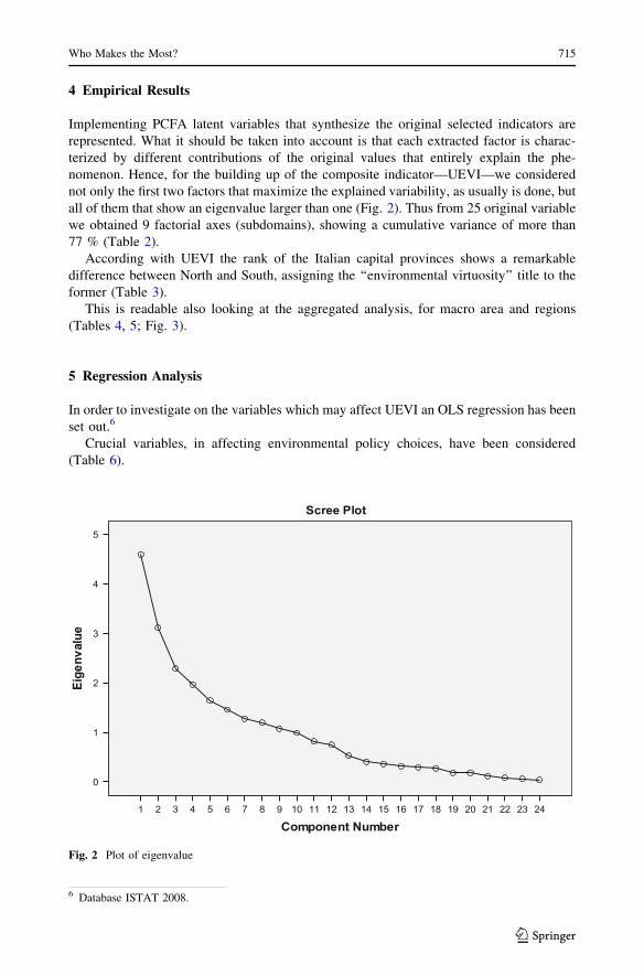
nomenon. Hence, for the building up of the composite indicator—UEVI—we considered

not only the first two factors that maximize the explained variability, as usually is done, but

all of them that show an eigenvalue larger than one (Fig. 2). Thus from 25 original variable

we obtained 9 factorial axes (subdomains), showing a cumulative variance of more than

77 % (Table 2).

According with UEVI the rank of the Italian capital provinces shows a remarkable

difference between North and South, assigning the ‘‘environmental virtuosity’’ title to the

former (Table 3).

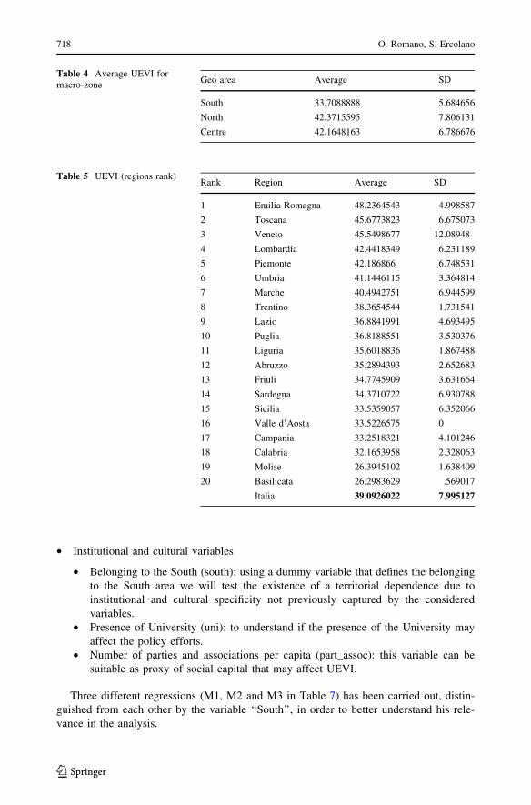
This is readable also looking at the aggregated analysis, for macro area and regions

(Tables 4, 5; Fig. 3).

5 Regression Analysis

In order to investigate on the variables which may affect UEVI an OLS regression has been

set out.6

Crucial variables, in affecting environmental policy choices, have been considered

(Table 6).

Fig. 2 Plot of eigenvalue

6 Database ISTAT 2008.


123

Variables have been divided in 3 sectors, as follows:

• Socio-economic variables (labels used in the tables of results in brackets):

• Gross domestic product per-capita (GDP pc): this variable is used as proxy of

economic development of the cities.

• Young aged population (pop0_14): this variable represents the share of the

population in the age 0–14 over the whole.7

• Density (den_pop): usually demographic pressure make harder the actions to be

undertaken by decision makers and it may affect in a negative way the efforts to be

carried out.

• Physical variables

• Surface (surf): this variable can be suitable to understand if the city size affects the

environmental-friendly level of policies.

• Altimetric zone (alt zone): the difference in the altimetry may affect UEVI.

Table 2 The factorial axes

Component

1 2 3 4 5 6 7 8 9

Ped .059 -.249 .602 .382 .066 -.134 .178 -.006 .196

Pist .480 .302 -.011 .356 .231 .142 .085 .398 -.067

Dep .102 .022 -.052 -.052 -.025 .759 .193 -.060 .050

Erog -.218 -.028 -.041 -.002 -.025 -.132 -.745 -.502 -.058

PEC .255 .030 .555 -.099 -.451 -.088 -.243 -.155 .057

Tel .275 .499 .224 .306 .101 .332 -.261 .283 -.230

PST -.068 .179 -.090 .130 -.047 .061 .461 -.155 -.290

PSF -.300 -.150 -.207 -.141 -.035 .541 .076 -.087 .492

Rum1 .155 .780 .220 -.088 -.075 -.005 .047 .009 .256

Rum2 .030 .898 .052 .041 .062 .012 .148 .011 -.060

Rum3 -.224 .806 -.045 .038 .000 -.238 .034 -.155 -.063

PUT .255 .066 .141 .142 .133 .021 .731 -.244 -.109

PV .017 .102 .020 .226 -.120 -.030 -.219 .076 .835

Diff .876 -.032 -.003 .357 -.005 -.003 .100 .017 -.013

Disc -.485 -.034 -.012 -.814 .111 .037 -.131 .029 .002

Inc .080 .037 .030 .909 -.100 -.126 .079 .081 .159

Comp .847 .009 -.120 -.013 -.031 -.155 .112 .022 .046

Rec .555 -.147 .109 .393 -.071 .267 .099 .390 -.172

Tras1 -.082 .096 .885 -.006 .019 -.167 .084 .054 -.021

Tras2 -.128 .274 .813 -.020 .176 .085 -.031 .078 -.107

Inq .358 .235 .172 .068 .082 -.674 .224 .059 .301

Cent_pc .103 -.153 .013 -.026 .863 -.026 -.025 -.052 -.016

Cent_d -.102 .224 .143 -.163 .812 -.075 .078 -.087 -.091

Sup_PM10 .042 -.084 .038 .040 -.132 -.183 -.128 .885 .088

7 The aim is to verify if UEVI can be affected by a younger population.


123

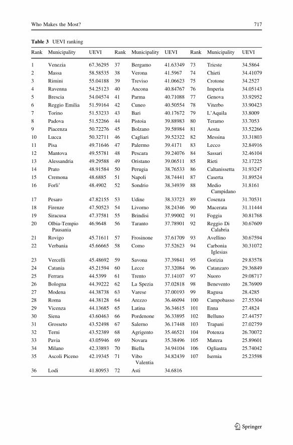
Table 3 UEVI ranking

Rank Municipality UEVI Rank Municipality UEVI Rank Municipality UEVI

1 Venezia 67.36295 37 Bergamo 41.63349 73 Trieste 34.5864

2 Massa 58.58535 38 Verona 41.5967 74 Chieti 34.41079

3 Rimini 55.04188 39 Treviso 41.06623 75 Crotone 34.2527

4 Ravenna 54.25123 40 Ancona 40.84767 76 Imperia 34.05143

5 Brescia 54.04574 41 Parma 40.71088 77 Genova 33.92952

6 Reggio Emilia 51.59164 42 Cuneo 40.50554 78 Viterbo 33.90423

7 Torino 51.53233 43 Bari 40.17672 79 L’Aquila 33.8009

8 Padova 51.52266 44 Pistoia 39.88983 80 Teramo 33.7053

9 Piacenza 50.72276 45 Bolzano 39.58984 81 Aosta 33.52266

10 Lucca 50.32711 46 Cagliari 39.52322 82 Messina 33.31803

11 Pisa 49.71646 47 Palermo 39.4171 83 Lecco 32.84916

12 Mantova 49.55781 48 Pescara 39.24076 84 Sassari 32.46104

13 Alessandria 49.29588 49 Oristano 39.06511 85 Rieti 32.17225

14 Prato 48.91584 50 Perugia 38.76533 86 Caltanissetta 31.93247

15 Cremona 48.6885 51 Napoli 38.74441 87 Caserta 31.89524

16 Forli’ 48.4902 52 Sondrio 38.34939 88 MedioCampidano

31.8161

17 Pesaro 47.82155 53 Udine 38.33723 89 Cosenza 31.70531

18 Firenze 47.50523 54 Livorno 38.24346 90 Macerata 31.11444

19 Siracusa 47.37581 55 Brindisi 37.99002 91 Foggia 30.81768

20 Olbia-TempioPausania

46.9648 56 Taranto 37.78901 92 Reggio DiCalabria

30.67609

21 Rovigo 45.71611 57 Frosinone 37.61709 93 Avellino 30.67594

22 Verbania 45.66665 58 Como 37.52623 94 CarboniaIglesias

30.31072

23 Vercelli 45.48692 59 Savona 37.39841 95 Gorizia 29.83578

24 Catania 45.21594 60 Lecce 37.32084 96 Catanzaro 29.36849

25 Ferrara 44.5399 61 Trento 37.14107 97 Nuoro 29.08717

26 Bologna 44.39222 62 La Spezia 37.02818 98 Benevento 28.76909

27 Modena 44.38738 63 Varese 37.00193 99 Ragusa 28.4285

28 Roma 44.38128 64 Arezzo 36.46094 100 Campobasso 27.55304

29 Vicenza 44.13685 65 Latina 36.34615 101 Enna 27.4824

30 Siena 43.60463 66 Pordenone 36.33895 102 Belluno 27.44757

31 Grosseto 43.52498 67 Salerno 36.17448 103 Trapani 27.02759

32 Terni 43.52389 68 Agrigento 35.46521 104 Potenza 26.70072

33 Pavia 43.05946 69 Novara 35.38496 105 Matera 25.89601

34 Milano 42.33893 70 Biella 34.94104 106 Ogliastra 25.74042

35 Ascoli Piceno 42.19345 71 ViboValentia

34.82439 107 Isernia 25.23598

36 Lodi 41.80953 72 Asti 34.6816


123

• Institutional and cultural variables

• Belonging to the South (south): using a dummy variable that defines the belonging

to the South area we will test the existence of a territorial dependence due to

institutional and cultural specificity not previously captured by the considered

variables.

• Presence of University (uni): to understand if the presence of the University may

affect the policy efforts.

• Number of parties and associations per capita (part_assoc): this variable can be

suitable as proxy of social capital that may affect UEVI.

Three different regressions (M1, M2 and M3 in Table 7) has been carried out, distin-

guished from each other by the variable ‘‘South’’, in order to better understand his rele-

vance in the analysis.

Table 4 Average UEVI formacro-zone

Geo area Average SD

South 33.7088888 5.684656

North 42.3715595 7.806131

Centre 42.1648163 6.786676

Table 5 UEVI (regions rank)Rank Region Average SD

1 Emilia Romagna 48.2364543 4.998587

2 Toscana 45.6773823 6.675073

3 Veneto 45.5498677 12.08948

4 Lombardia 42.4418349 6.231189

5 Piemonte 42.186866 6.748531

6 Umbria 41.1446115 3.364814

7 Marche 40.4942751 6.944599

8 Trentino 38.3654544 1.731541

9 Lazio 36.8841991 4.693495

10 Puglia 36.8188551 3.530376

11 Liguria 35.6018836 1.867488

12 Abruzzo 35.2894393 2.652683

13 Friuli 34.7745909 3.631664

14 Sardegna 34.3710722 6.930788

15 Sicilia 33.5359057 6.352066

16 Valle d’Aosta 33.5226575 0

17 Campania 33.2518321 4.101246

18 Calabria 32.1653958 2.328063

19 Molise 26.3945102 1.638409

20 Basilicata 26.2983629 .569017

Italia 39.0926022 7.995127


123

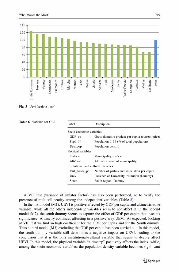
A VIF test (variance of inflator factor) has also been performed, so to verify the

presence of multicollinearity among the independent variables (Table 8).

In the first model (M1), UEVI is positive affected by GDP per capita and altimetric zone

variable, while all the others independent variables seem to not affect it. In the second

model (M2), the south dummy seems to capture the effect of GDP per capita that loses its

significance. Altimetry continues affecting in a positive way UEVI. As expected, looking

at VIF test we find an high coefficient for the GDP per capita and for the South dummy.

Thus a third model (M3) excluding the GDP per capita has been carried out. In this model,

the south dummy variable still determines a negative impact on UEVI, leading to the

conclusion that it is the only institutional-cultural variable that seems to deeply affect

UEVI. In this model, the physical variable ‘‘altimetry’’ positively affects the index, while,

among the socio-economic variables, the population density variable becomes significant

Fig. 3 Uevi (regions rank)

Table 6 Variable for OLSLabel Description

Socio-economic variables

GDP_pc Gross domestic product per capita (current price)

Pop0_14 Population 0–14 (% of total population)

Den_pop Population density

Physical variables

Surface Municipality surface

AltZone Altimetric zone of municipality

Institutional and cultural variables

Part_Assoc_pc Number of parties and association per capita

Univ Presence of University institution (Dummy)

South South region (Dummy)


123

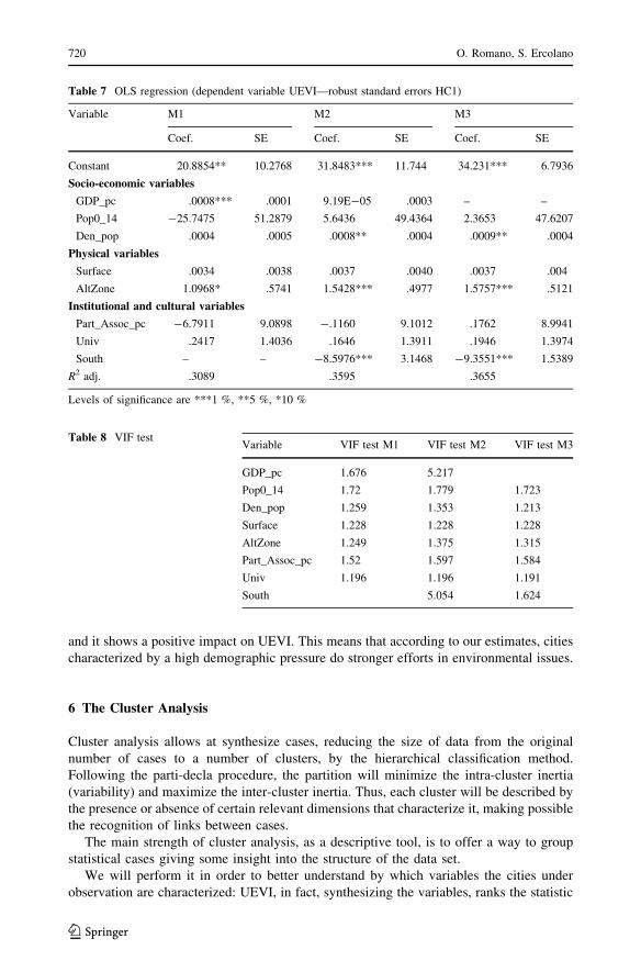
and it shows a positive impact on UEVI. This means that according to our estimates, cities

characterized by a high demographic pressure do stronger efforts in environmental issues.

6 The Cluster Analysis

Cluster analysis allows at synthesize cases, reducing the size of data from the original

number of cases to a number of clusters, by the hierarchical classification method.

Following the parti-decla procedure, the partition will minimize the intra-cluster inertia

(variability) and maximize the inter-cluster inertia. Thus, each cluster will be described by

the presence or absence of certain relevant dimensions that characterize it, making possible

the recognition of links between cases.

The main strength of cluster analysis, as a descriptive tool, is to offer a way to group

statistical cases giving some insight into the structure of the data set.

We will perform it in order to better understand by which variables the cities under

observation are characterized: UEVI, in fact, synthesizing the variables, ranks the statistic

Table 7 OLS regression (dependent variable UEVI—robust standard errors HC1)

Variable M1 M2 M3

Coef. SE Coef. SE Coef. SE

Constant 20.8854** 10.2768 31.8483*** 11.744 34.231*** 6.7936

Socio-economic variables

GDP_pc .0008*** .0001 9.19E-05 .0003 – –

Pop0_14 -25.7475 51.2879 5.6436 49.4364 2.3653 47.6207

Den_pop .0004 .0005 .0008** .0004 .0009** .0004

Physical variables

Surface .0034 .0038 .0037 .0040 .0037 .004

AltZone 1.0968* .5741 1.5428*** .4977 1.5757*** .5121

Institutional and cultural variables

Part_Assoc_pc -6.7911 9.0898 -.1160 9.1012 .1762 8.9941

Univ .2417 1.4036 .1646 1.3911 .1946 1.3974

South – – -8.5976*** 3.1468 -9.3551*** 1.5389

R2 adj. .3089 .3595 .3655

Levels of significance are ***1 %, **5 %, *10 %

Table 8 VIF testVariable VIF test M1 VIF test M2 VIF test M3

GDP_pc 1.676 5.217

Pop0_14 1.72 1.779 1.723

Den_pop 1.259 1.353 1.213

Surface 1.228 1.228 1.228

AltZone 1.249 1.375 1.315

Part_Assoc_pc 1.52 1.597 1.584

Univ 1.196 1.196 1.191

South 5.054 1.624


123

units representing a good tool for benchmarking purpose. Cluster analysis can be used,

instead to investigate the negative aspects that put the cities in the lowest places of the

ranking, giving important signals to decision makers.

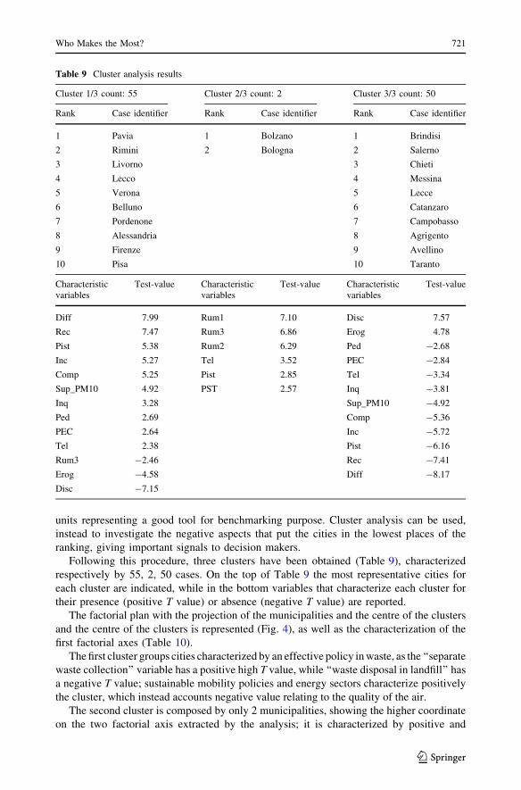
Following this procedure, three clusters have been obtained (Table 9), characterized

respectively by 55, 2, 50 cases. On the top of Table 9 the most representative cities for

each cluster are indicated, while in the bottom variables that characterize each cluster for

their presence (positive T value) or absence (negative T value) are reported.

The factorial plan with the projection of the municipalities and the centre of the clusters

and the centre of the clusters is represented (Fig. 4), as well as the characterization of the

first factorial axes (Table 10).

The first cluster groups cities characterized by an effective policy in waste, as the ‘‘separate

waste collection’’ variable has a positive high T value, while ‘‘waste disposal in landfill’’ has

a negative T value; sustainable mobility policies and energy sectors characterize positively

the cluster, which instead accounts negative value relating to the quality of the air.

The second cluster is composed by only 2 municipalities, showing the higher coordinate

on the two factorial axis extracted by the analysis; it is characterized by positive and

Table 9 Cluster analysis results

Cluster 1/3 count: 55 Cluster 2/3 count: 2 Cluster 3/3 count: 50

Rank Case identifier Rank Case identifier Rank Case identifier

1 Pavia 1 Bolzano 1 Brindisi

2 Rimini 2 Bologna 2 Salerno

3 Livorno 3 Chieti

4 Lecco 4 Messina

5 Verona 5 Lecce

6 Belluno 6 Catanzaro

7 Pordenone 7 Campobasso

8 Alessandria 8 Agrigento

9 Firenze 9 Avellino

10 Pisa 10 Taranto

Characteristicvariables

Test-value Characteristicvariables

Test-value Characteristicvariables

Test-value

Diff 7.99 Rum1 7.10 Disc 7.57

Rec 7.47 Rum3 6.86 Erog 4.78

Pist 5.38 Rum2 6.29 Ped -2.68

Inc 5.27 Tel 3.52 PEC -2.84

Comp 5.25 Pist 2.85 Tel -3.34

Sup_PM10 4.92 PST 2.57 Inq -3.81

Inq 3.28 Sup_PM10 -4.92

Ped 2.69 Comp -5.36

PEC 2.64 Inc -5.72

Tel 2.38 Pist -6.16

Rum3 -2.46 Rec -7.41

Erog -4.58 Diff -8.17

Disc -7.15


123

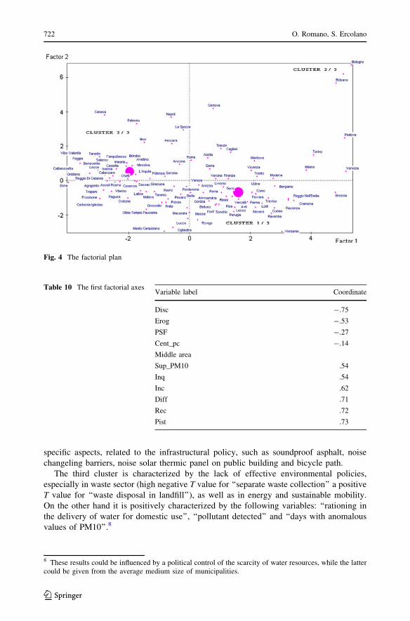
specific aspects, related to the infrastructural policy, such as soundproof asphalt, noise

changeling barriers, noise solar thermic panel on public building and bicycle path.

The third cluster is characterized by the lack of effective environmental policies,

especially in waste sector (high negative T value for ‘‘separate waste collection’’ a positive

T value for ‘‘waste disposal in landfill’’), as well as in energy and sustainable mobility.

On the other hand it is positively characterized by the following variables: ‘‘rationing in

the delivery of water for domestic use’’, ‘‘pollutant detected’’ and ‘‘days with anomalous

values of PM10’’.8

Fig. 4 The factorial plan

Table 10 The first factorial axesVariable label Coordinate

Disc -.75

Erog -.53

PSF -.27

Cent_pc -.14

Middle area

Sup_PM10 .54

Inq .54

Inc .62

Diff .71

Rec .72

Pist .73

8 These results could be influenced by a political control of the scarcity of water resources, while the lattercould be given from the average medium size of municipalities.


123

7 Conclusions

Starting from the concept of ‘‘virtuosity’’ we have build a composite indicator (UEVI), in

order to capture the ability of local authorities to tackle environmental problems within

the urban context. Our local focus is due to the fact that decisions taken at this scale of

governance affect not only surrounding contexts, but are likely to have more widespread

effects. It is the opinion of the authors that the overused label of ‘‘sustainable’’ used by

cities which have developed environmental-friendly policies, should be substituted by a

more appropriate one, such as ‘‘virtuous’’ in order to indicate the local government’s

efforts in using an ecosystem approach to urban management.

This paper has developed a theoretical framework to underpin the construction of a

composite indicator, and through this presented a clear picture of the virtuosity of the

capital provinces of Italy. Its relevance consists not only in its purpose, but also in the

methodology that has been used: the multivariate analysis and PCA in particular, which

overcome problems found in other techniques, related to the choice of weights.

After having obtained the ranking of the cities that basically divided Italy in two: virtuous

or not, coinciding strikingly with geographical location, we investigated the determinants that

affect the ranking by OLS analysis. A set of socio economic variables coupled to location in

the south of Italy (dummy variable ‘‘south’’) have the greatest impact on the UEVI.

Finally, in order to better understand which variables characterize the cities under

observation and the type of interventions that might be undertaken, a cluster analysis was

performed. By dividing the cities in homogeneous groups is possible to figure out the

variables that positively or negatively characterize them. It transpires that interventions in

the waste and energy sectors contribute heavily to ‘‘virtuous’’ outcomes for a city. Cities

located in the highest position of the ranking belong mostly to the first cluster. It is

noticeable that the variables concerning the waste sector positively characterize them (high

positive t value for recycling activities for example), while cities located at the lowest

places of the ranking, corresponded to the third cluster, show a negative t value for the

disposal in landfill. This last group of cities uses widely landfill for treating waste, in

collection barely separate different kinds of waste, and have no treatment plants. Hence,

putting in practice eco-friendly modes of waste management, in particular, will ensure such

cities rise in the rankings.

Obviously several cities are distinguished not only by geophysics characteristics,

but also by the need of the population, priorities of local decision makers and budget

constraints. However because of national and international environmental standards to

be respected and because the awareness towards environmental issues, UEVI could be

employed as a useful tool in order to push the competition among cites in improving the

general state of the environment.

Acknowledgments This work is a result of continuous and shared ideas between the two authors; howeverSalvatore Ercolano wrote paragraphs 3,4,5, while Oriana Romano wrote paragraphs 1,2,6. We would liketo thank Professors Pietro Rostirolla, Amedeo Di Maio, John Sedgwick, Abay Mulatu and Dr. RintaroYamaguchi for the useful comments.

References

Adriaanse, A. (1993). Environmental policy performance indicators: A study on the development of indi-cators for environmental policy in the Netherlands. The Hague: SDV Publishers.


123

Atkinson, G. D., Dubourg, R., Hamilton, K., Munasignhe, M., Pearce, D. W., & Young, C. (1997). Mea-suring sustainable development: Macroeconomics and the environment. Cheltenham: Edward Elgar.

Bohringer, C. (2007). Measuring the immeasurable: A survey of sustainability indices. Ecological Eco-nomics, 63, 1–8.

Coco, G., & Russo, M. (2006). Using CATPCA to evaluate market regulation. In S. Zani, et al. (Eds.), Dataanalysis classification and the forward search (pp. 369–376). Berlin: Springer.

Ercolano, S., & Gaeta, G. L. (2012). (Re)assessing the power of purse. A new methodology for the analysisof the institutional capacity for legislative control over the budget. Journal of Dyses (forthcoming).

European Commission. (1994). Charter of European cities and towns towards sustainability. In Europeanconference on sustainable cities and towns, Aalborg, Denmark on May 27, 1994.

Helsinki City Urban Facts Office (2002). The core indicators for sustainable development in Helsinki.Agenda 21. Helsinki, Web publication, 2002:4

Isla, M. (1996). A review of the urban indicators experience and a proposal to overcome current situation.The application to the municipalities of the Barcelona Province. Departament d’Economıa AplicadaAutonomous, University of Barcelona.

Istat. (2009). Indicatori ambientali urbani. Roma: Servizio statistiche ambientali.Legambiente. (1994). Ecosistema urbano: Rapporto sulla qualita ambientale dei comuni capoluogo di

provincia. http://www.legambiente.eu/documenti/1989-1996/ecosistemaUrbano1994.pdf.Linting, M., Neurman, J. J., Groenen, P. J., & Van Der Koojj, A. J. (2007). Nonlinear principal components

analysis: Introduction and application. Physical Methods, 12(3), 336–358.Nardo, M., Saisana, M., Salltelli, A., & Tarantola, S. (2005). Tools for composite indicators building. Joint

Research Centre and Institute for the Protection and Security of the Citizen Econometrics andStatistical Support to Antifraud Unit I-21020 Ispra, VA, Italy.

Nicoletti, G., Scarpetta, S., & Boylaud, O. (2000). Summary indicators of product market regulation withan extension to employment protection legislation. OECD Economics Department working papersno. 226.

Niemeijer, D. (2002). Developing indicators for environmental policy: Data-driven and theory-drivenapproaches examined by example. Environmental Science & Policy, 5, 91–103.

Niemeijer, D., & de Groot, R. S. (2008). A conceptual framework for selecting environmental indicator sets.Ecological Indicators, 8, 14–25.

OECD. (1993). Core set of indicators for environmental performance reviews. A synthesis report by theGroup on the State of the Environment, Environmental monographs no. 83.

OECD, European Commission, Joint Research Centre (2008). Handbook on constructing composite indi-cators: Methodology and user guide, by Nardo, M. M. Saisana, A. Saltelli, and S. Tarantola (EC/JRC),A. Hoffman and E. Giovannini (OECD), Paris, OECD publication Code: 302008251E1.

Puolamaa, M., Kaplas, M. & Reinikainen T. (1996). Index of environmental friendliness: A methodologicalstudy. Helsinki: Statistics Finland/Eurostat.

Rapporto di Ambiente Italia. (2003). Verso un quadro della sostenibilita a livello locale—Indicatori comunieuropei (ICE), Roma.

Saisana, M., & Tarantola, S. (2002). State-of-the-art report on current methodologies and practices forcomposite indicator development. EUR report 20408 EN, European Commission, JRC-IPSC, Italy.

Saltelli, A. (2007). Composite indicators between analysis and advocacy. Social Indicators Research, 81,65–77.

Singh, R. K., Murty, H. R., Gupta, S. K., & Dikshit, A. K. (2009). An overview of sustainability assessmentmethodologies. Ecological Indicators, 5(3), 189–212.

Svedin, L. M. (2009). Organizational cooperation in crises. Farnham: Ashgate.UN Habitat. (2002). Global urban indicators database, version 2. Nairobi, Kenya: Global Urban Obser-

vatory, United Nations Human Settlements Programme.Zhang, M. (2002). Measuring urban sustainability in China. Thela thesis, Amsterdam.


123

http://www.legambiente.eu/documenti/1989-1996/ecosistemaUrbano1994.pdf

who makes the most? measuring the “urban environmental virtuosity”

Documents