White Dwarf Stars

After nuclear burning ceases, a post-AGB star rapidly becomes awhite dwarf. Although gravitational contraction will provide someluminosity for a while, the luminosity evolution of the star can bewell modeled as simple cooling for a highly conductive isothermal,degenerate core blanketed by a radiative non-degenerate envelope.

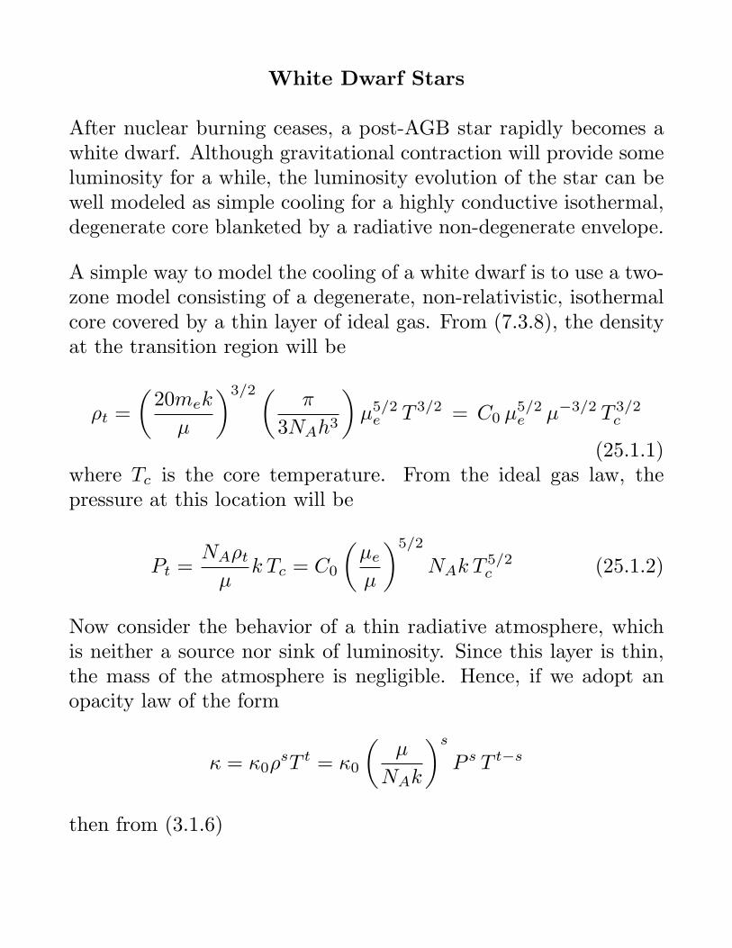
A simple way to model the cooling of a white dwarf is to use a two-zone model consisting of a degenerate, non-relativistic, isothermalcore covered by a thin layer of ideal gas. From (7.3.8), the densityat the transition region will be

ρt =

(20mek

µ

)3/2 (π

3NAh3

)µ5/2e T 3/2 = C0 µ

5/2e µ−3/2 T 3/2

c

(25.1.1)where Tc is the core temperature. From the ideal gas law, thepressure at this location will be

Pt =NAρtµ

k Tc = C0

(µe

µ

)5/2

NAk T5/2c (25.1.2)

Now consider the behavior of a thin radiative atmosphere, whichis neither a source nor sink of luminosity. Since this layer is thin,the mass of the atmosphere is negligible. Hence, if we adopt anopacity law of the form

κ = κ0ρsT t = κ0

(µ

NAk

)s

P s T t−s

then from (3.1.6)

∇rad =P

T

dT

dP=

3κ

16πacG

LMT

P

T 4

=3κ0

16πacG

(µ

NAk

)s LMT

P s+1 T t−s−4

= C1 µs

(L

MT

)P s+1 T t−s−4 (25.1.3)

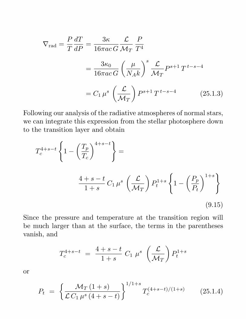
Following our analysis of the radiative atmospheres of normal stars,we can integrate this expression from the stellar photosphere downto the transition layer and obtain

T 4+s−tc

{1−

(Tp

Tc

)4+s−t}

=

4 + s− t

1 + sC1 µ

s

(L

MT

)P 1+st

{1−

(Pp

Pt

)1+s}

(9.15)

Since the pressure and temperature at the transition region willbe much larger than at the surface, the terms in the parenthesesvanish, and

T 4+s−tc =

4 + s− t

1 + sC1 µs

(L

MT

)P 1+st

or

Pt =

{MT (1 + s)

LC1 µs (4 + s− t)

}1/1+s

T (4+s−t)/(1+s)c (25.1.4)

If we equate this equation to (25.1.2), we get an expression for theluminosity and temperature of the star in terms of the temperatureof the central core

C0

(µe

µ

) 52

NAk T52c =

{MT (1 + s)

LC1 µs (4 + s− t)

} 11+s

T(4+s−t)(1+s)

c =⇒

L =

{1 + s

C1 (4 + s− t)

}{µ−5/2e

C0NAk

}1+s

µ(3s+5)/2 MT T (3−3s−2t)/2c

(25.1.5)For a Kramers opacity which is dominated by bound-free absorp-tion, s = 1, t = −7/2, and κ0 ≈ 4 × 1025 cm2-g−1. Moreover, by(5.1.3), (5.1.6), and (5.1.7), µe ≈ 2, and µ ≈ 1.75, so

L = C2 MT T 7/2c (25.1.6)

(where C2 ∼ 5 × 10−30, if the mass and luminosity are in solarunits).

Next, consider the reaction of the core to its energy loss. The coreis already degenerate, so gravitational contraction will not occur.However the core will cool, and the amount of this cooling will begiven by the specific heat.

L = −dE

dt= −cV M

dTc

dt(25.1.7)

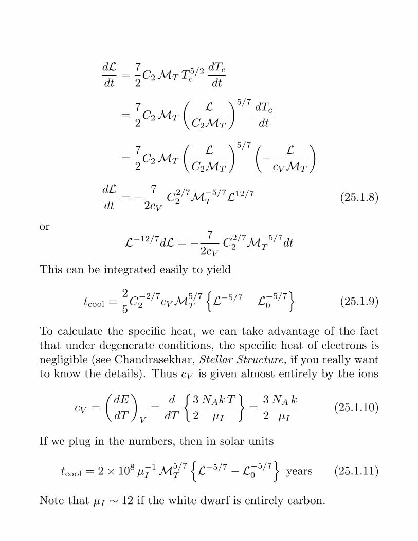
From this, we can compute the cooling curve of the star. If we takethe derivative of (25.1.6) with respect to time, write it in terms ofluminosity and mass, and then substitute in for the temperaturederivative using (25.1.7), then

dLdt

=7

2C2 MT T 5/2

c

dTc

dt

=7

2C2 MT

(L

C2MT

)5/7dTc

dt

=7

2C2 MT

(L

C2MT

)5/7 (− LcV MT

)dLdt

= − 7

2cVC

2/72 M−5/7

T L12/7 (25.1.8)

or

L−12/7dL = − 7

2cVC

2/72 M−5/7

T dt

This can be integrated easily to yield

tcool =2

5C

−2/72 cV M5/7

T

{L−5/7 − L−5/7

0

}(25.1.9)

To calculate the specific heat, we can take advantage of the factthat under degenerate conditions, the specific heat of electrons isnegligible (see Chandrasekhar, Stellar Structure, if you really wantto know the details). Thus cV is given almost entirely by the ions

cV =

(dE

dT

)V

=d

dT

{3

2

NAk T

µI

}=

3

2

NA k

µI(25.1.10)

If we plug in the numbers, then in solar units

tcool = 2× 108 µ−1I M5/7

T

{L−5/7 − L−5/7

0

}years (25.1.11)

Note that µI ∼ 12 if the white dwarf is entirely carbon.

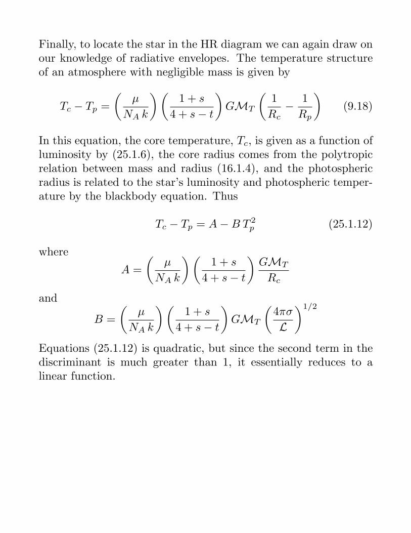
Finally, to locate the star in the HR diagram we can again draw onour knowledge of radiative envelopes. The temperature structureof an atmosphere with negligible mass is given by

Tc − Tp =

(µ

NA k

)(1 + s

4 + s− t

)GMT

(1

Rc− 1

Rp

)(9.18)

In this equation, the core temperature, Tc, is given as a function ofluminosity by (25.1.6), the core radius comes from the polytropicrelation between mass and radius (16.1.4), and the photosphericradius is related to the star’s luminosity and photospheric temper-ature by the blackbody equation. Thus

Tc − Tp = A−B T 2p (25.1.12)

where

A =

(µ

NA k

)(1 + s

4 + s− t

)GMT

Rc

and

B =

(µ

NA k

)(1 + s

4 + s− t

)GMT

(4πσ

L

)1/2

Equations (25.1.12) is quadratic, but since the second term in thediscriminant is much greater than 1, it essentially reduces to alinear function.

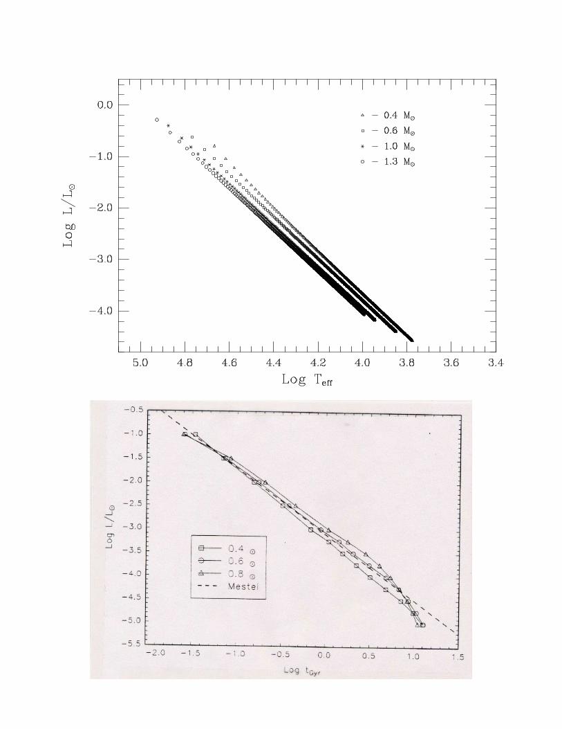
This simple cooling law reproduces the observed distribution ofwhite dwarfs quite well. The cooling timescale derived above is afactor of ∼ 2 too fast (which probably comes from our definition ofthe transition region). However, the behavior of the cooling curve,and its position in the HR diagram is accurate. There are severalfeatures to note:

• The starting point for the calculation was L = 1000L⊙ at t = 0,but this makes very little difference to the calculation. (This canbe seen from (25.1.9) quite easily.) Thus the term L0 is usuallydropped from cooling formulae.

• Each tick mark in the figure represents 107 years. Note that whitedwarfs fade quickly at first; but after a while, their evolution isexceedingly slow. The last point plotted is after 1010 years; thus thecoolest white dwarfs in existence should still have a temperatureof >∼ 6500 K.

• The cooling curves for different mass stars are offset slightly. Bymatching the position of a white dwarf (or an evolved planetarynebula central star) with its position in the HR diagram, it is pos-sible to estimate its mass.

• From a white dwarf’s location in the HR diagram, it is possible toestimate how long it has been cooling, i.e., its age. By examiningthe luminosity function of white dwarfs in the Milky Way, it ispossible to get an independent estimate of the age of the Galaxy.

Realistic Models of White Dwarfs

There are a number of processes associated with white dwarfs thatare difficult to model. As a result, our understanding of theircooling is not as complete as we would like.

• The composition of white dwarfs is not well known. Most areclearly a mixture of carbon and oxygen, but the proportion of thesetwo elements is not well constrained. A few massive white dwarfsin nova systems show evidence of heavy elements; neon-oxygen-magnesium novae are relatively common.

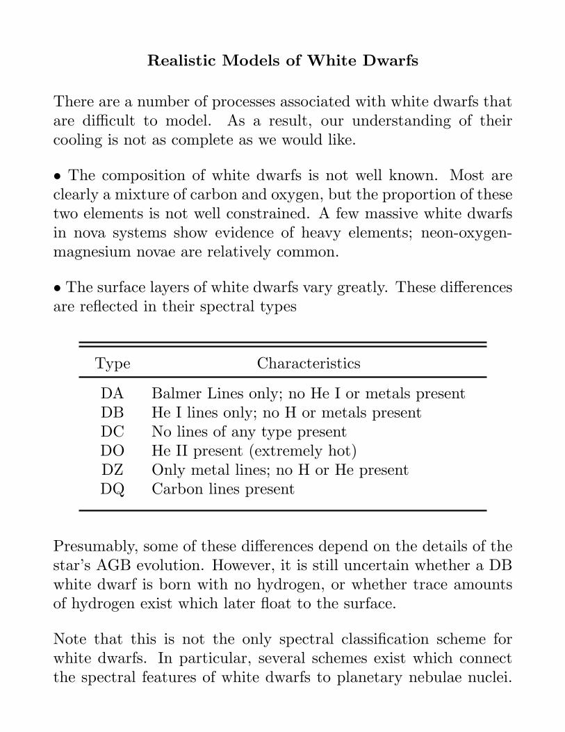
• The surface layers of white dwarfs vary greatly. These differencesare reflected in their spectral types

Type Characteristics

DA Balmer Lines only; no He I or metals presentDB He I lines only; no H or metals presentDC No lines of any type presentDO He II present (extremely hot)DZ Only metal lines; no H or He presentDQ Carbon lines present

Presumably, some of these differences depend on the details of thestar’s AGB evolution. However, it is still uncertain whether a DBwhite dwarf is born with no hydrogen, or whether trace amountsof hydrogen exist which later float to the surface.

Note that this is not the only spectral classification scheme forwhite dwarfs. In particular, several schemes exist which connectthe spectral features of white dwarfs to planetary nebulae nuclei.

Unfortunately, the classification criteria are not standard. (In fact,many are self-contradictory!)

• As a white dwarf cools, solid-state effects becomes more im-portant (i.e., crystallization can occur). This greatly changes theequation of state.

•Many intermediate temperature white dwarf atmospheres do con-vect. Thus, simple radiative energy transport is not applicable toall white dwarfs. This changes the cooling curve somewhat, andcan change the surface abundances.

• It is an observed fact that the overwhelming majority of whitedwarfs have masses near ∼ 0.6M⊙, and there is very little disper-sion about this mean. This is usually attributed to a very slowlyvarying initial-mass final-mass relation for stars. But the actualdata is poor.

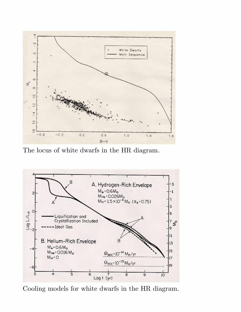
The locus of white dwarfs in the HR diagram.

Cooling models for white dwarfs in the HR diagram.

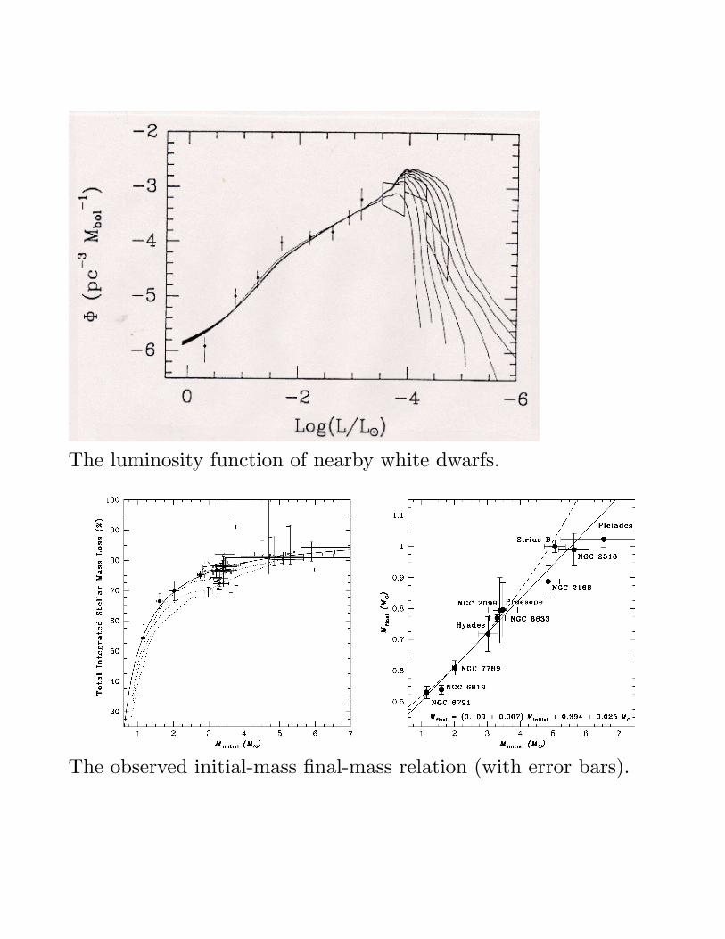
The luminosity function of nearby white dwarfs.

The observed initial-mass final-mass relation (with error bars).

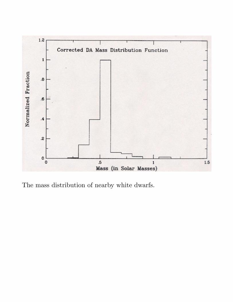
The mass distribution of nearby white dwarfs.

Pulsating Stars

Every star in the HR diagram has a natural (fundamental) fre-quency for pulsation. To understand this, consider a pulsation asthe resonance of a sound wave. To first order, the speed at whicha sound wave traverses a star is

vs =

(γP

ρ

)1/2

(25.2.1)

where γ is the ratio of the specific heats. Now for a first approxi-mation, let’s assume a constant density star. The pressure at anypoint in such a star can be found by directly integrating

dP

dr= −MGρ

r2= −

(4

3πr3ρ

)Gρ

r2= −4

3πGρ2r

to yield

P (r) =2

3πGρ2

(R2 − r2

)where R is the stellar radius. The period of pulsation is thenroughly the time it takes for this sound wave to cross the star, i.e.,

Π ≈ 2

∫ R

0

dr

vs≈ 2

∫ R

0

(2

3γπGρ(R2 − r2)

)−1/2

dr ≈(

3π

2γGρ

)1/2

(25.2.2)There is only one variable in this equation — the density. To agood approximation, this holds true for all stars pulsating (radi-ally) in the fundamental mode: the period of the star is inverselyproportional to the square root of the average density. In otherwords

Π⟨ρ⟩1/2 = Q (25.2.3)

where Q is some constant.

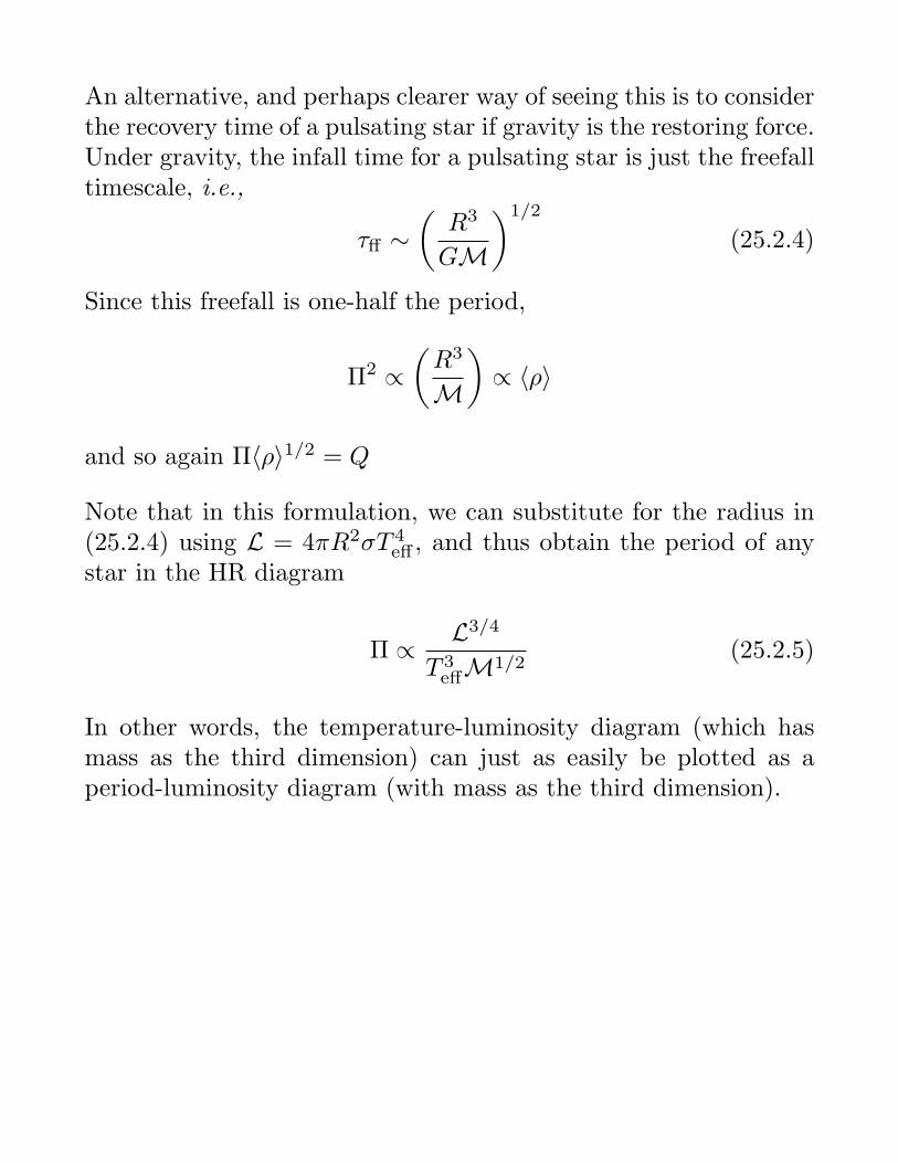
An alternative, and perhaps clearer way of seeing this is to considerthe recovery time of a pulsating star if gravity is the restoring force.Under gravity, the infall time for a pulsating star is just the freefalltimescale, i.e.,

τff ∼(

R3

GM

)1/2

(25.2.4)

Since this freefall is one-half the period,

Π2 ∝(R3

M

)∝ ⟨ρ⟩

and so again Π⟨ρ⟩1/2 = Q

Note that in this formulation, we can substitute for the radius in(25.2.4) using L = 4πR2σT 4

eff , and thus obtain the period of anystar in the HR diagram

Π ∝ L3/4

T 3effM1/2

(25.2.5)

In other words, the temperature-luminosity diagram (which hasmass as the third dimension) can just as easily be plotted as aperiod-luminosity diagram (with mass as the third dimension).

Pulsation Mechanisms

In theory, there are three mechanisms which can cause mechanicalinstability in a star.

The ϵ mechanism: If the center of the star is compressed slightly,the nuclear reaction rates will go up, causing an increase in expan-sion. The expansion can then decrease the reaction rates, cool thecentral core, and cause contraction.

The κ mechanism: Suppose the opacity in some region of astar were to increase with density. Upon compression, the materialwould absorb more energy, heat up, and expand. In the ensuingexpansion, the opacity would decrease, heat would be lost from thesystem, and the material would fall back down. Pulsation wouldbe driven by changes in the opacity.

The γ mechanism: If, during compression, a region of the starwere to heat up less than its surroundings, heat would flow intoit. This heat could then cause the region to expand, and in theexpansion, the excess heat could be returned to its surroundings.The specific heat of the gas would drive pulsation.

In practice, the ϵ mechanism is not an effective way of driving pul-sations in normal stars. Although the core is unstable to ϵ-drivenpulsations, the amplitudes involved are not large enough to be de-tectable. The exception occurs in extremely massive (M > 90M⊙)stars, where the sensitivity of the ϵ-mechanism to temperature isenough to cause large oscillations and possibly disrupt the star.

Under most circumstances, stars have Kramer-law type opacities,and have an ideal-gas equation of state. Thus

κ ∝ ρT−3.5 ∝ ρ−2.5

which means that the κ mechanism will not work. However, intransition regions where stellar material is only partially ionized,the energy produced by compression will go into increasing the ion-ization fraction, rather than the thermal motion of the particles.When this happens, the κ mechanism is effective. Moreover, dur-ing compression, this region of partial ionization will be somewhatcooler than normal, due to the energy lost to the ionization pro-cess. Thus, heat will flow into the region and the γ mechanism willalso operate.

The κ and γ mechanisms can only drive pulsations in certain re-gions of the HR diagram. For pulsations to occur, there must be aregion in the star where a substantial fraction of the hydrogen (orhelium) is partially ionized. If the star is too hot, this zone will belocated very near the stellar surface, where the density is too lowto drive stellar oscillations. On the other hand, if the star is toocool, convection will occur at the surface. Since the energy trans-ported by convection is proportional to the amount of matter beingmoved, during compression more material will move, the heat flowwill increase, and the effectiveness of the energy damming will bedecreased. Thus, there is an “instability strip” in the HR diagram.

(Actually, there are several instability strips in the HR diagram.The classic instability strip associated with Cepheids, RR Lyr stars,δ Scuti (main sequence) stars, and ZZ Ceti white dwarfs, is due tothe partial ionization (and recombination) of He II. At the extremered edge of the HR diagram is the hydrogen and He I instabilitystrip; in this area are Mira stars and other Long Period Variables.Far to the blue in the HR diagram is an instability strip associ-ated with the partial ionization of carbon and oxygen. Of course,this latter zone is not important for normal stars, since CO is usu-ally not abundant enough to drive pulsations. However, hydrogen-deficient post-AGB stars (K1-16 type planetary nebula nuclei andPG 1159 white dwarfs) are susceptible to oscillations.)

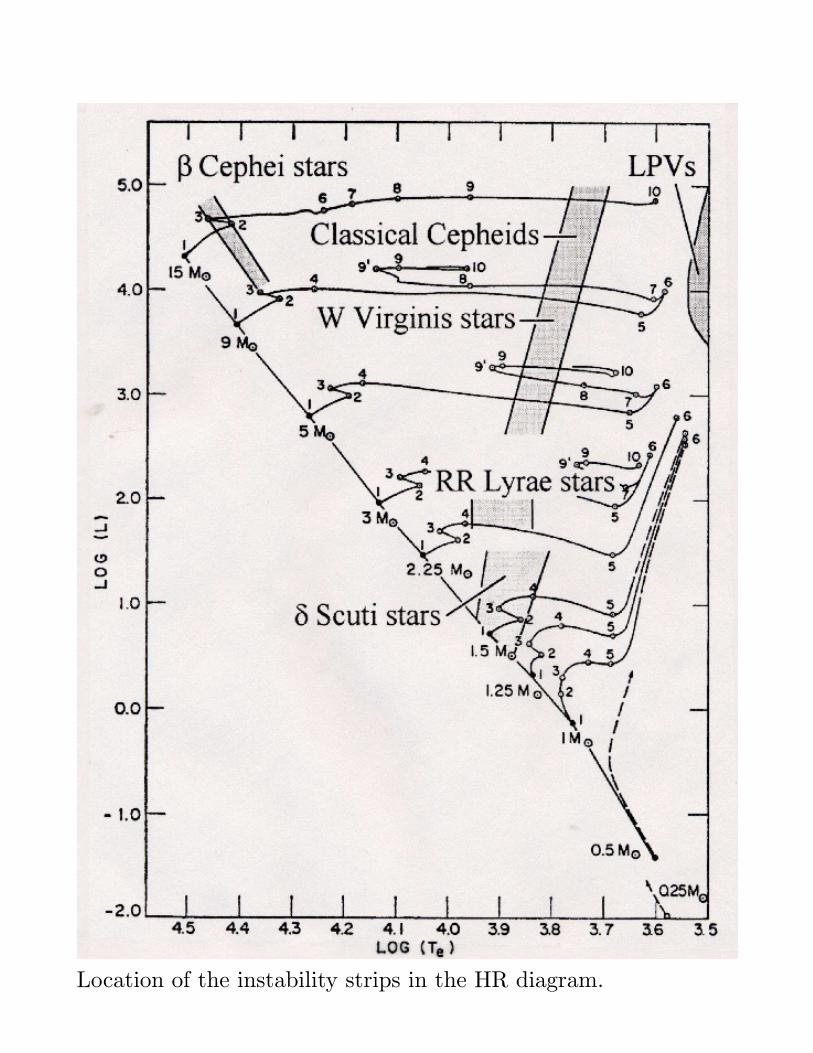
Location of the instability strips in the HR diagram.