where’s the money‽ an investigation into the whereabouts ... · where’s the money‽ an...

Where’s the Money‽ An Investigation into the Whereabouts

and Uses of Australian Banknotes

Richard Finlay, Andrew Staib and Max Wakefield

Research Discussion Paper

R DP 2018-12

Figures in this publication were generated using Mathematica.

The contents of this publication shall not be reproduced, sold or distributed without the prior consent of the Reserve Bank of Australia and, where applicable, the prior consent of the external source concerned. Requests for consent should be sent to the Secretary of the Bank at the email address shown above.

ISSN 1448-5109 (Online)

The Discussion Paper series is intended to make the results of the current economic research within the Reserve Bank available to other economists. Its aim is to present preliminary results of research so as to encourage discussion and comment. Views expressed in this paper are those of the authors and not necessarily those of the Reserve Bank. Use of any results from this paper should clearly attribute the work to the authors and not to the Reserve Bank of Australia.

Enquiries:

Phone: +61 2 9551 9830 Facsimile: +61 2 9551 8033 Email: [email protected] Website: https://www.rba.gov.au

Where’s the Money‽ An Investigation into the Whereabouts and Uses of Australian Banknotes

Richard Finlay, Andrew Staib and Max Wakefield

Research Discussion Paper 2018-12

December 2018

Note Issue Department Reserve Bank of Australia

The authors would like to thank Ben Fung, James Holloway, Melissa Hope, Tony Richards,

John Simon and a number of cash industry participants for useful comments, suggestions and

discussions. Any remaining errors are the responsibility of the authors alone. The views in this paper

are those of the authors and do not necessarily reflect the views of the Reserve Bank of Australia.

Authors: finlayr, staiba and wakefieldm at domain rba.gov.au

Media Office: [email protected]

Abstract

The Reserve Bank of Australia is the sole issuer and redeemer of Australian banknotes. This means

that we know exactly how many banknotes have ever been printed and issued to the public, and

how many banknotes, at the end of their life, have been returned to the Reserve Bank and destroyed.

Between issuance and destruction, however, there is little public information about where banknotes

go or what they are used for. Such information would be of interest for a number of reasons,

including to aid in forecasting future banknote demand, and to assess the extent to which banknotes

are used to facilitate illegal activities or avoid tax obligations. To address this we use a range of

techniques to estimate the whereabouts and uses of Australian banknotes. The techniques that we

employ suggest that, of total outstanding banknotes: 15–35 per cent are used to facilitate legitimate

transactions; roughly half to three-quarters are hoarded as a store of wealth or for other purposes,

of which we can allocate 10–20 percentage points to domestic hoarding and up to 15 percentage

points to international hoarding; 4–8 per cent are used in the shadow economy; and 5–10 per cent

are lost.

JEL Classification Numbers: E41, E58

Keywords: banknotes, lost money, transactional demand, hoarding, shadow economy

Table of Contents

1. Introduction 1

2. Background Data and International Comparisons 2

3. Lost Banknotes 5

4. Cash Used in Legitimate Transactions 6

4.1 The Counting Method 7

4.1.1 Method 7

4.1.2 Results 7

4.2 The Banknote Life Method 8

4.2.1 Method 8

4.2.2 Results 12

4.3 The Banknote Processing Frequency Method 13

4.4 The Velocity Method 14

4.4.1 The value of cash payments 15

4.4.2 The velocity of transactional cash 16

4.4.3 Results 17

4.5 The Seasonality Method 19

4.5.1 Method 19

4.5.2 Results 21

4.5.3 Assessment 22

4.6 Overall Assessment 23

5. The Shadow Economy 24

5.1 ABS Estimates for 2009/10 Applied to 2017/18 GDP Figures 25

5.2 Black Economy Taskforce Estimates 25

5.3 New Estimates of Cash Used in the Drug Trade 26

5.3.1 Estimates of cash used to purchase illicit drugs 26

5.3.2 Estimates of cash held by drug suppliers 28

5.4 Overall Assessment and International Comparison 29

6. Hoarding 30

6.1 One Minus Transactional Demand 31

6.2 Domestic Hoarding: Fire-damaged Banknote Claims 31

6.2.1 Results 32

6.3 Domestic Hoarding: Results from the Consumer Payments Survey 33

6.4 International Hoarding: Outflow Less Inflow 33

6.5 Overall Assessment 34

7. Conclusion 35

Appendix A : Ground-up Calculations 37

Appendix B : Banknote Life Calculations 42

Appendix C : Velocity Calculations 43

References 44

1. Introduction

Relatively strong growth in the value of outstanding banknotes has been a consistent feature of the

Australian economy for many decades.1 For example, over the 10 years to June 2018, year-ended

growth in the value of outstanding banknotes averaged 6 per cent, bringing the total value to

approximately $76 billion. Ongoing growth has occurred despite an observable shift away from cash

as a means of payment, a phenomenon observed in many countries.2 To explain these diverging

trends, it has been argued that the share of cash used for non-transactional purposes, particularly

as a store of value, must be increasing.3

This paper aims to provide an estimate of where the approximately $76 billion worth of Australian

banknotes – or $3,000 per Australian – are held, and for what purposes these banknotes are used.

Broadly speaking, at any point in time the stock of outstanding banknotes can be considered to fall

into one of the following categories:

1. banknotes used to facilitate legitimate day-to-day transactions in Australia;

2. banknotes that are held, either domestically or overseas, as a store of value, for emergency

liquidity or other such purposes (referred to as hoarding);

3. banknotes used in the shadow economy (either to conceal legal transactions to avoid tax, to

pay for illegal goods or to store wealth generated by the sale of illegal goods); or

4. banknotes that have been lost or destroyed.

Individual banknotes, of course, are able to move between these different categories over time.

Cash, by its nature, is anonymous and hard to trace, and so any attempt to estimate where

outstanding banknotes are and what they are used for, including that made here, is bound to be an

approximation at best. To mitigate this, where possible we use a variety of techniques to estimate

the same quantity, with the idea being that, if the errors of each technique are imperfectly correlated,

then the range of estimates produced will provide a better indication of the truth than any individual

method could. To preview results, our estimates suggest that:

1. around 15 to 35 per cent of outstanding banknotes are used to facilitate legitimate transactions

within Australia;

2. roughly half to three-quarters of outstanding banknotes are hoarded; of this, we can allocate

10–20 percentage points to domestic hoarding, and up to 15 percentage points to international

hoarding;

1 We will use the terms ‘banknotes’ and ‘cash’ interchangeably throughout the paper.

2 For example, Doyle et al (2017) document that in 2016, electronic payments surpassed cash as the most common

payment method.

3 See, for example, Davies et al (2016) and Flannigan and Staib (2017), as well as Flannigan and Parsons (2018) for a

comparison of trends in Australia, Canada and the United Kingdom.

2

3. around 4 to 8 per cent of outstanding banknotes are used in the shadow economy, of which,

3–5 per cent are used to conceal legal transactions, 1–2 per cent are used to purchase illegal

drugs, and up to 1 per cent are used to store profits from illegal activity; and

4. around 5 to 10 per cent of outstanding banknotes are actually lost.

Given the number of dissimilar methods that we use to estimate transactional demand, all of which

give broadly similar results, we can have reasonable confidence that the true stock of transactional

banknotes used for legitimate purposes falls somewhere within our estimated range. Our estimates

of lost cash accord with international experience, and so again seem unlikely to be too far off the

mark; and while our ‘transactional’ shadow economy estimates are less certain, our transactional

demand estimates mentioned earlier – some of which implicitly include transactional cash used in

the shadow economy – suggest that they are at least of the right order of magnitude. By implication

we can have reasonable confidence that our overall hoarding estimate of roughly half to

three-quarters of outstanding banknotes is broadly accurate.

The allocation of total hoarded banknotes to domestic hoarding, international hoarding, and the

concealment of profits from illegal activity, however, remains quite uncertain. Our domestic hoarding

estimate, which is based on a survey of households, is almost certainly too low: the distribution of

domestically hoarded banknotes is likely to have a long right tail (that is, most people have little to

no hoarded banknotes, while a few people have very large hoards), which makes it difficult to

accurately estimate average hoarding; and people who choose to hoard banknotes are, for security

or other reasons, unlikely to advertise this fact and so may not tell survey collectors their true

holdings. Our estimates of overseas hoarding and the hoarding of profits from illegal activity are also

very uncertain, and it is possible that these are larger than suggested above.

2. Background Data and International Comparisons

Before commencing our detailed discussion on where Australian banknotes are and for what

purposes they are used, we briefly outline some background information and key trends.

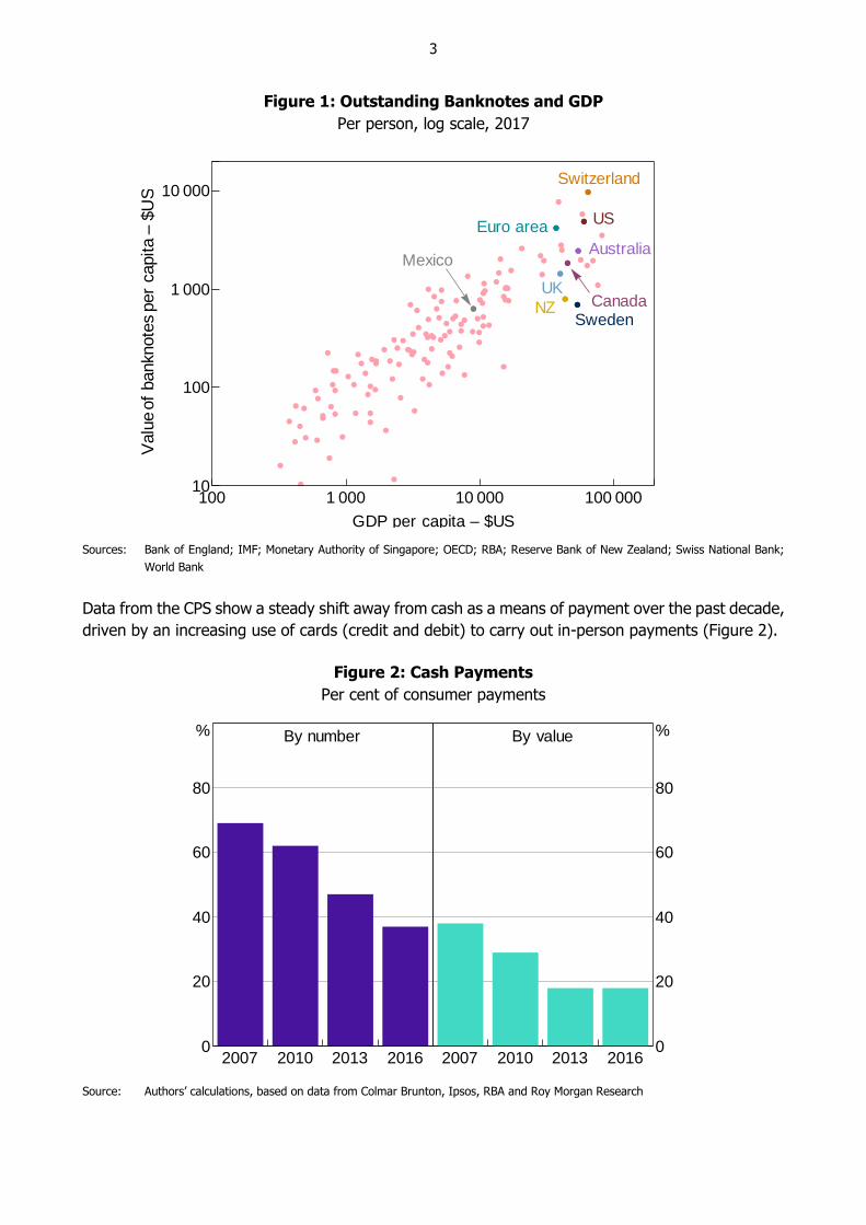
As noted earlier, there are roughly $3,000 worth of banknotes outstanding per person in Australia.

Although this figure might seem high, Australia is by no means an outlier amongst other comparable

countries (Figure 1). By denomination, the vast majority of the value of outstanding banknotes –

93 per cent as at June 2018 – is accounted for by the $50 and $100 denominations, split roughly

evenly between the two. By contrast, $5 banknotes represent just 1 per cent of outstanding value,

$10 banknotes represent 2 per cent, and $20 banknotes represent 4 per cent. As such, although

this paper considers banknotes in general rather than high denomination banknotes in particular,

trends in the latter drive results in the former.

We now outline some key trends evident in the Reserve Bank’s Consumer Payments Survey (CPS).4

The survey, conducted triennially, provides the Reserve Bank with a nationally representative dataset

of the payment habits of Australian consumers and how these habits have changed over time. It is

a key source of information on cash use.

4 The Reserve Bank conducted the survey in 2007, 2010, 2013 and 2016; the next survey is planned for 2019.

3

Figure 1: Outstanding Banknotes and GDP

Per person, log scale, 2017

Sources: Bank of England; IMF; Monetary Authority of Singapore; OECD; RBA; Reserve Bank of New Zealand; Swiss National Bank;

World Bank

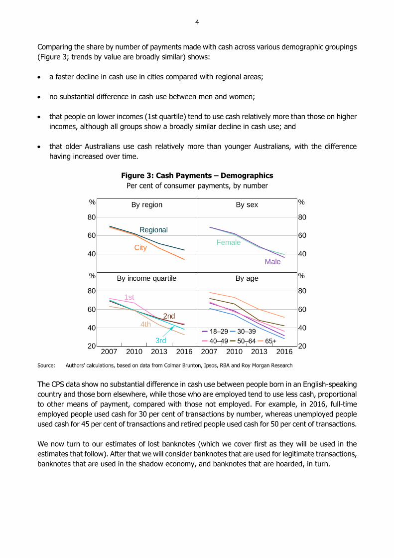
Data from the CPS show a steady shift away from cash as a means of payment over the past decade,

driven by an increasing use of cards (credit and debit) to carry out in-person payments (Figure 2).

Figure 2: Cash Payments

Per cent of consumer payments

Source: Authors’ calculations, based on data from Colmar Brunton, Ipsos, RBA and Roy Morgan Research

100 1 000 10 000 100 00010

100

1 000

10 000

GDP per capita – $US

Valu

eof

banknote

sper

capita–

$U

S

Switzerland

US

NZSweden

AustraliaMexico

CanadaUK

Euro area

By number

2007 2010 2013 20160

20

40

60

80

% By value

2007 2010 2013 20160

20

40

60

80

%

4

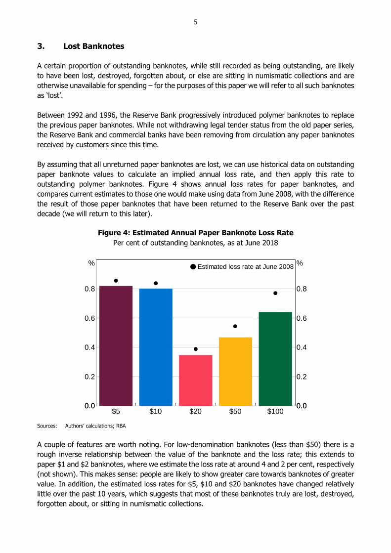
Comparing the share by number of payments made with cash across various demographic groupings

(Figure 3; trends by value are broadly similar) shows:

a faster decline in cash use in cities compared with regional areas;

no substantial difference in cash use between men and women;

that people on lower incomes (1st quartile) tend to use cash relatively more than those on higher

incomes, although all groups show a broadly similar decline in cash use; and

that older Australians use cash relatively more than younger Australians, with the difference

having increased over time.

Figure 3: Cash Payments – Demographics

Per cent of consumer payments, by number

Source: Authors’ calculations, based on data from Colmar Brunton, Ipsos, RBA and Roy Morgan Research

The CPS data show no substantial difference in cash use between people born in an English-speaking

country and those born elsewhere, while those who are employed tend to use less cash, proportional

to other means of payment, compared with those not employed. For example, in 2016, full-time

employed people used cash for 30 per cent of transactions by number, whereas unemployed people

used cash for 45 per cent of transactions and retired people used cash for 50 per cent of transactions.

We now turn to our estimates of lost banknotes (which we cover first as they will be used in the

estimates that follow). After that we will consider banknotes that are used for legitimate transactions,

banknotes that are used in the shadow economy, and banknotes that are hoarded, in turn.

By region

40

60

80

%

City

Regional

By sex

40

60

80

%

Male

Female

By income quartile

2007 2010 2013 201620

40

60

80

%

1st

4th

3rd

2nd

By age

18–29 30–39

40–49 50–64 65+

2007 2010 2013 201620

40

60

80

%

5

3. Lost Banknotes

A certain proportion of outstanding banknotes, while still recorded as being outstanding, are likely

to have been lost, destroyed, forgotten about, or else are sitting in numismatic collections and are

otherwise unavailable for spending – for the purposes of this paper we will refer to all such banknotes

as ‘lost’.

Between 1992 and 1996, the Reserve Bank progressively introduced polymer banknotes to replace

the previous paper banknotes. While not withdrawing legal tender status from the old paper series,

the Reserve Bank and commercial banks have been removing from circulation any paper banknotes

received by customers since this time.

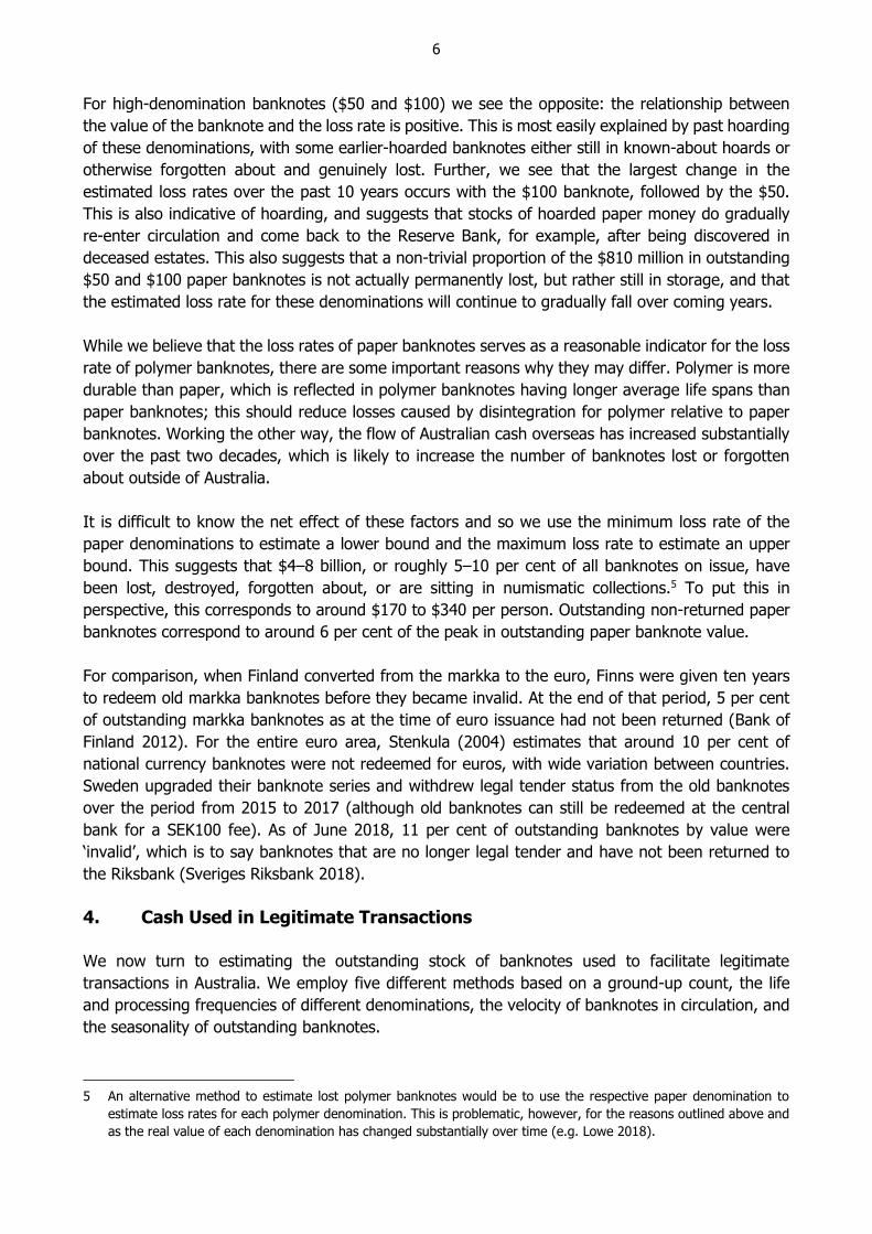
By assuming that all unreturned paper banknotes are lost, we can use historical data on outstanding

paper banknote values to calculate an implied annual loss rate, and then apply this rate to

outstanding polymer banknotes. Figure 4 shows annual loss rates for paper banknotes, and

compares current estimates to those one would make using data from June 2008, with the difference

the result of those paper banknotes that have been returned to the Reserve Bank over the past

decade (we will return to this later).

Figure 4: Estimated Annual Paper Banknote Loss Rate

Per cent of outstanding banknotes, as at June 2018

Sources: Authors’ calculations; RBA

A couple of features are worth noting. For low-denomination banknotes (less than $50) there is a

rough inverse relationship between the value of the banknote and the loss rate; this extends to

paper $1 and $2 banknotes, where we estimate the loss rate at around 4 and 2 per cent, respectively

(not shown). This makes sense: people are likely to show greater care towards banknotes of greater

value. In addition, the estimated loss rates for $5, $10 and $20 banknotes have changed relatively

little over the past 10 years, which suggests that most of these banknotes truly are lost, destroyed,

forgotten about, or sitting in numismatic collections.

Estimated loss rate at June 2008

$5 $10 $20 $50 $1000.00.0

0.2

0.4

0.6

0.8

%

0.00.0

0.2

0.4

0.6

0.8

%

6

For high-denomination banknotes ($50 and $100) we see the opposite: the relationship between

the value of the banknote and the loss rate is positive. This is most easily explained by past hoarding

of these denominations, with some earlier-hoarded banknotes either still in known-about hoards or

otherwise forgotten about and genuinely lost. Further, we see that the largest change in the

estimated loss rates over the past 10 years occurs with the $100 banknote, followed by the $50.

This is also indicative of hoarding, and suggests that stocks of hoarded paper money do gradually

re-enter circulation and come back to the Reserve Bank, for example, after being discovered in

deceased estates. This also suggests that a non-trivial proportion of the $810 million in outstanding

$50 and $100 paper banknotes is not actually permanently lost, but rather still in storage, and that

the estimated loss rate for these denominations will continue to gradually fall over coming years.

While we believe that the loss rates of paper banknotes serves as a reasonable indicator for the loss

rate of polymer banknotes, there are some important reasons why they may differ. Polymer is more

durable than paper, which is reflected in polymer banknotes having longer average life spans than

paper banknotes; this should reduce losses caused by disintegration for polymer relative to paper

banknotes. Working the other way, the flow of Australian cash overseas has increased substantially

over the past two decades, which is likely to increase the number of banknotes lost or forgotten

about outside of Australia.

It is difficult to know the net effect of these factors and so we use the minimum loss rate of the

paper denominations to estimate a lower bound and the maximum loss rate to estimate an upper

bound. This suggests that $4–8 billion, or roughly 5–10 per cent of all banknotes on issue, have

been lost, destroyed, forgotten about, or are sitting in numismatic collections.5 To put this in

perspective, this corresponds to around $170 to $340 per person. Outstanding non-returned paper

banknotes correspond to around 6 per cent of the peak in outstanding paper banknote value.

For comparison, when Finland converted from the markka to the euro, Finns were given ten years

to redeem old markka banknotes before they became invalid. At the end of that period, 5 per cent

of outstanding markka banknotes as at the time of euro issuance had not been returned (Bank of

Finland 2012). For the entire euro area, Stenkula (2004) estimates that around 10 per cent of

national currency banknotes were not redeemed for euros, with wide variation between countries.

Sweden upgraded their banknote series and withdrew legal tender status from the old banknotes

over the period from 2015 to 2017 (although old banknotes can still be redeemed at the central

bank for a SEK100 fee). As of June 2018, 11 per cent of outstanding banknotes by value were

‘invalid’, which is to say banknotes that are no longer legal tender and have not been returned to

the Riksbank (Sveriges Riksbank 2018).

4. Cash Used in Legitimate Transactions

We now turn to estimating the outstanding stock of banknotes used to facilitate legitimate

transactions in Australia. We employ five different methods based on a ground-up count, the life

and processing frequencies of different denominations, the velocity of banknotes in circulation, and

the seasonality of outstanding banknotes.

5 An alternative method to estimate lost polymer banknotes would be to use the respective paper denomination to

estimate loss rates for each polymer denomination. This is problematic, however, for the reasons outlined above and

as the real value of each denomination has changed substantially over time (e.g. Lowe 2018).

trim://D18%2f115396/?db=RC&view

7

4.1 The Counting Method

4.1.1 Method

The first approach is a direct one. We estimate the transactional stock of cash from the ground up.

This means estimating the stock of cash held in various physical locations that we consider to be

part of the transactional stock, and aggregating them to form an economy-wide estimate. This

calculation by necessity relies on a number of assumptions, and will miss any cash held in locations

not directly considered. Despite these drawbacks the approach is useful as it provides a broad sense-

check on other estimates arrived at through more abstract means, and also offers a tangible basis

to think about the transactional stock of cash.

The locations we consider to be part of the transactional stock are listed in Table 1. We use two

approaches to estimate the stock of cash held in each of these locations:

Estimating the number of particular locations (e.g. the number of tills) and multiplying this by

an estimated average amount held per location. Where appropriate, these estimates are

deflated/inflated by other series (e.g. population, inflation or a measure of economic activity).

Converting flow data to a stock by making assumptions about the velocity of cash through a

particular location.

Table 1: Transactional Cash

Physical location

Location Description

Wallets Cash held by consumers on their person.

Financial institution

holdings

Cash held by financial institutions including in ATMs, bank branches and cash depots, as

well as cash in transit.

Tills and self-service check-

outs

Cash held in tills and cash-accepting self-service check-outs at the start of business. This

is the minimum stock of banknotes that is held at all times. It does not include cash held

due to an increase in stocks from consumers’ cash expenditure.

Unbanked business takings Cash held by businesses due to consumers’ cash expenditure that has not been banked.

Gaming machines Cash held in gaming machines (e.g. poker machines).

Tourists Cash held by tourists in Australia or about to enter Australia. This includes cash sourced

overseas prior to entering Australia and cash sourced domestically after entering Australia.

Cash held by overseas foreign exchange businesses that service tourists about to enter

Australia is also included here.

A more detailed explanation of the specific methodology used to estimate the stock of cash held in

each location can be found in Appendix A.

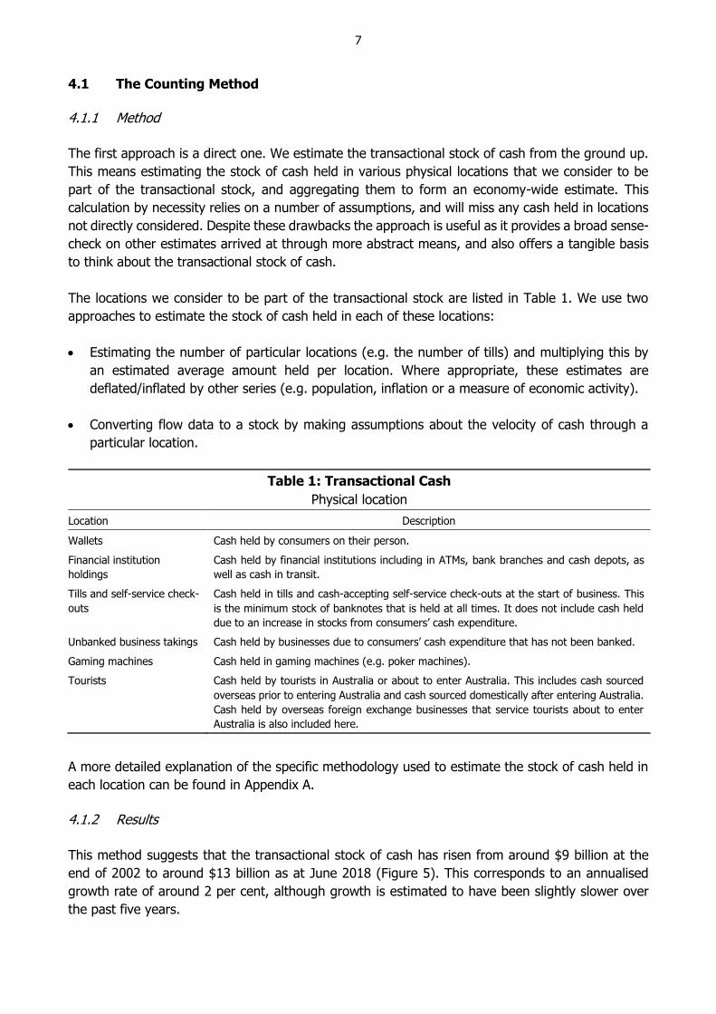
4.1.2 Results

This method suggests that the transactional stock of cash has risen from around $9 billion at the

end of 2002 to around $13 billion as at June 2018 (Figure 5). This corresponds to an annualised

growth rate of around 2 per cent, although growth is estimated to have been slightly slower over

the past five years.

8

Figure 5: Transactional Banknote Stock Estimates

Ground-up method

Sources: ABS; Australian Payments Network; Authors’ calculations, based on data from Colmar Brunton, Ipsos, RBA and Roy Morgan

Research; Queensland Treasury; Tourism Research Australia; Wesfarmers; Woolworths Group

In dollar terms, financial institution holdings drove most of the increase in the total transactional

stock, although most components have grown since 2002. In fact, the only component that is

estimated not to have grown since 2002 is unbanked business takings. This follows from relatively

stable cash expenditure, as growth in total nominal spending has been offset by changes in

consumers’ payment preferences.

While the transactional stock estimated using this method has increased since 2002, it has not kept

pace with the increase in total outstanding banknotes, which has grown at around 6 per cent per

annum over this period. As a result, the transactional stock’s share in total outstanding banknotes

is estimated to have fallen from 30 per cent to a little under 20 per cent according to this method.

4.2 The Banknote Life Method

4.2.1 Method

Banknotes reach the end of their lives (become ‘unfit’) for two main reasons: excessive inkwear,

which will tend to increase in a relatively linear fashion with banknote use; and mechanical defects

such as tears, which can be thought of as random events that can occur at any stage, but whose

cumulative probability of having occurred also increases with use. We measure banknote life as the

average number of banknotes outstanding over a given period, divided by the number of banknotes

that have been deemed unfit over the same period, and choose a five-year period to average over

201420102006 20180

2

4

6

8

10

12

$b

0

2

4

6

8

10

12

$b

Wallets

Financial institution holdings

Tills and self-serve check-outs

Unbanked business takings

Gaming machines

Tourists

9

in order to reduce undue volatility.6 When performing this calculation we also adjust the number of

outstanding banknotes for our estimate of lost banknotes, using the midpoint of our 5–10 per cent

loss range.

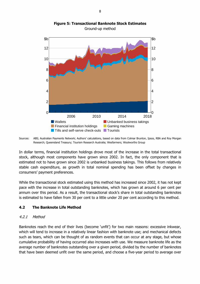
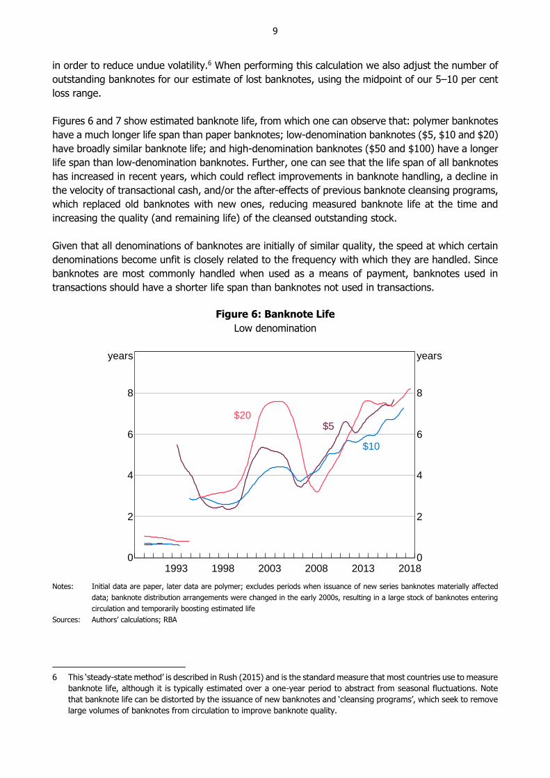
Figures 6 and 7 show estimated banknote life, from which one can observe that: polymer banknotes

have a much longer life span than paper banknotes; low-denomination banknotes ($5, $10 and $20)

have broadly similar banknote life; and high-denomination banknotes ($50 and $100) have a longer

life span than low-denomination banknotes. Further, one can see that the life span of all banknotes

has increased in recent years, which could reflect improvements in banknote handling, a decline in

the velocity of transactional cash, and/or the after-effects of previous banknote cleansing programs,

which replaced old banknotes with new ones, reducing measured banknote life at the time and

increasing the quality (and remaining life) of the cleansed outstanding stock.

Given that all denominations of banknotes are initially of similar quality, the speed at which certain

denominations become unfit is closely related to the frequency with which they are handled. Since

banknotes are most commonly handled when used as a means of payment, banknotes used in

transactions should have a shorter life span than banknotes not used in transactions.

Figure 6: Banknote Life

Low denomination

Notes: Initial data are paper, later data are polymer; excludes periods when issuance of new series banknotes materially affected

data; banknote distribution arrangements were changed in the early 2000s, resulting in a large stock of banknotes entering

circulation and temporarily boosting estimated life


6 This ‘steady-state method’ is described in Rush (2015) and is the standard measure that most countries use to measure

banknote life, although it is typically estimated over a one-year period to abstract from seasonal fluctuations. Note

that banknote life can be distorted by the issuance of new banknotes and ‘cleansing programs’, which seek to remove

large volumes of banknotes from circulation to improve banknote quality.

20132008200319981993 20180

2

4

6

8

years

0

2

4

6

8

years

$10

$5$20

10

Figure 7: Banknote Life

High denomination


data; banknote distribution arrangements were changed in the early 2000s, resulting in a large stock of banknotes entering

circulation and temporarily boosting estimated life


For our estimates, we assume that low-denomination banknotes are used only for transactional

purposes. Although this may not be exactly true, it is likely to be a close approximation of reality as

the low value of these banknotes relative to the $50 and $100 make them an inefficient store of

value. That they all have similar life spans further supports the idea that they are used for similar

purposes (Figure 6). For example, if the $20 was hoarded significantly more than the $10, we would

expect that to manifest in a longer life for $20 banknotes, whereas this is not the case. Nonetheless,

we note that if a large volume of low-denomination banknotes are actually used for non-transactional

purposes, our estimates of the transactional stock will be upwardly biased.

Moreover, we assume that all banknotes used for transactional purposes are handled an equal

number of times and with equal care. This assumption is arguably more tenuous: high-denomination

banknotes used for transactions may be treated with more care than low-denomination banknotes

and, further, may be handled less frequently because they are less likely to be given as change

(e.g. the $100 will never be given as change). To the extent that this assumption does not hold, our

estimates of the transactional stock will be downwardly biased.

Working the other way, even if transactional high-denomination banknotes are used less frequently

for payments than low-denomination banknotes, high-denomination banknotes are more likely to

pass through ATMs and other banknote processing machines, and so be quality-screened and

‘handled’ in that way; if the process of being stocked in and withdrawn from ATMs is particularly

wearing, and/or the more frequent quality-screening allows these banknotes to be withdrawn from

circulation earlier than lower denomination banknotes that are quality-screened less often, this will

upwardly bias our transactional stock estimates.

50

100

150

200

years

50

100

150

200

years

$100

20132008200319981993 20180

10

20

30

years

0

10

20

30

years

$50

11

If the net effect of all these potential issues had large effects on banknote life, we might expect this

to show up in the $20, which is both less likely to be given as change than the $5 and $10, and is

far more likely to be quality-screened and passed through ATMs. The fact that the $20 has a very

similar life to the $5 and $10 therefore provides some comfort these issues are not materially

affecting our results.

Given these assumptions, any ‘excess life’ of high-denomination banknotes, relative to low-

denomination banknotes, can be attributed to the non-transactional uses that they facilitate

(e.g. store of value), and so can be used to estimate the split between transactional and non-

transactional cash. In particular, assuming that transactional high-denomination banknotes have the

same life span as lower denomination banknotes (all of which are assumed to be used for

transactions), the excess life of $50 and $100 banknotes, relative to the average life of the lower

denominations, divided by the average life of the higher denominations, gives the estimated share

of non-transactional high-denomination banknotes. Intuitively, imagine that one in four

$50 banknotes is used for transactions and three in four are hoarded. The hoarded banknotes will

never become unfit as they lie untouched. The transactional $50 banknotes should become unfit at

the same rate as the lower denominations, assuming that they are handled in a similar fashion.

Accordingly, the ratio of total to unfit banknotes over a given period (i.e. ‘banknote life’) should be

four times higher for $50 banknotes relative to the lower denominations, and the above calculation

will give a result of three-quarters (see Appendix B for the mathematics). Boeschoten (1992) uses

a similar method to estimate hoarding in the Netherlands, while Bartzsch, Rösl and Seitz (2011)

employ the method using the differing average ages of German and French banknotes, rather than

between denominations, to estimate the transactional share of German banknotes.

To ensure that the issuance of new series NGB banknotes has no effect on our estimates, we exclude

denominations from our calculations from the date of NGB issuance. We also exclude estimates for

periods when the issuance of the polymer banknotes materially affected the data (the mid 1990s),

but include data around the early 2000s when a change to banknote distribution arrangements

artificially boosted estimated banknote life (as all denominations were affected, the net result on our

transactional stock estimates is small; see Figure 8); we make no attempt to adjust for earlier

banknote cleansing programs, with the five-year averaging of banknote life that we use designed to

mitigate various idiosyncratic shocks to individual banknote life series.

12

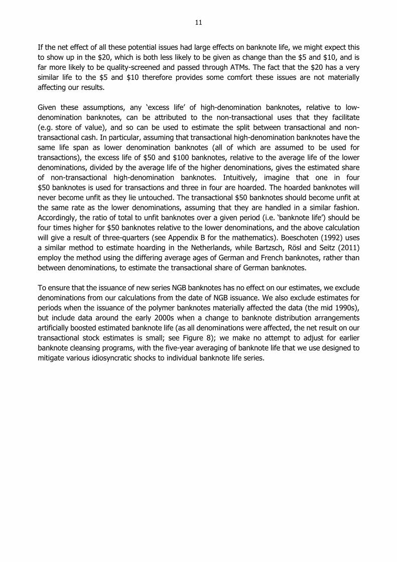
Figure 8: Transactional Banknote Estimates

Banknote life method, per cent of outstanding banknotes


data


4.2.2 Results

Over the past three decades we estimate that: the share of $100 banknotes used for transactions

has fallen from around 20 per cent to just 3 per cent; the share of $50 banknotes used for

transactions has fallen from around 35 per cent to 25 per cent; and the transactional share by value

of all banknotes has fallen from around 45 per cent to around 20 per cent (Figure 8). Excluding the

$100 banknote, which is overwhelmingly used for non-transactional purposes, we estimate that the

transactional share of the lower four denominations is around 35 per cent. Given that this method

makes no distinction between cash used for legitimate and illegitimate purposes, subtracting an

estimated 5 per cent of cash used for shadow economy transactions (see Section 5.4) suggests that

the overall transactional share, restricted to legal transactions, is around 15 per cent of outstanding

banknotes.

If we relax the assumption that all transactional banknotes should have equal life and instead assume

that transactional $50 and $100 banknotes last twice as long as the lower denominations, say,

perhaps due to more careful handling for example, then the implied transactional share of $50 and

$100 banknotes is double that given in Figure 8, and the overall transactional share of outstanding

banknotes falls from 65 per cent three decades ago to 35 per cent today, or around 30 per cent

after subtracting cash used in shadow economy transactions.

As noted, the above figures assume that around 7½ per cent of banknotes recorded as outstanding

have actually been lost, and adjust for this. If we do not adjust for lost banknotes, the transactional

share estimates above are boosted by around 2 percentage points.

20132008200319981993 20180

10

20

30

40

%

0

10

20

30

40

%

$100

$50

All denominations

13

4.3 The Banknote Processing Frequency Method

One can apply the same idea used in Section 4.2 to data on the frequency with which different

banknote denominations are processed by cash depots. In particular, cash depots process and

fitness-sort banknotes lodged by commercial banks and large retailers, and importantly do not

process any banknotes that are hoarded or otherwise not part of the transactional stock of cash.

Thus, broadly speaking, only the transactional stock of banknotes passes through cash depots, and

the rate at which banknotes pass through depots is an indication of transactional cash use.

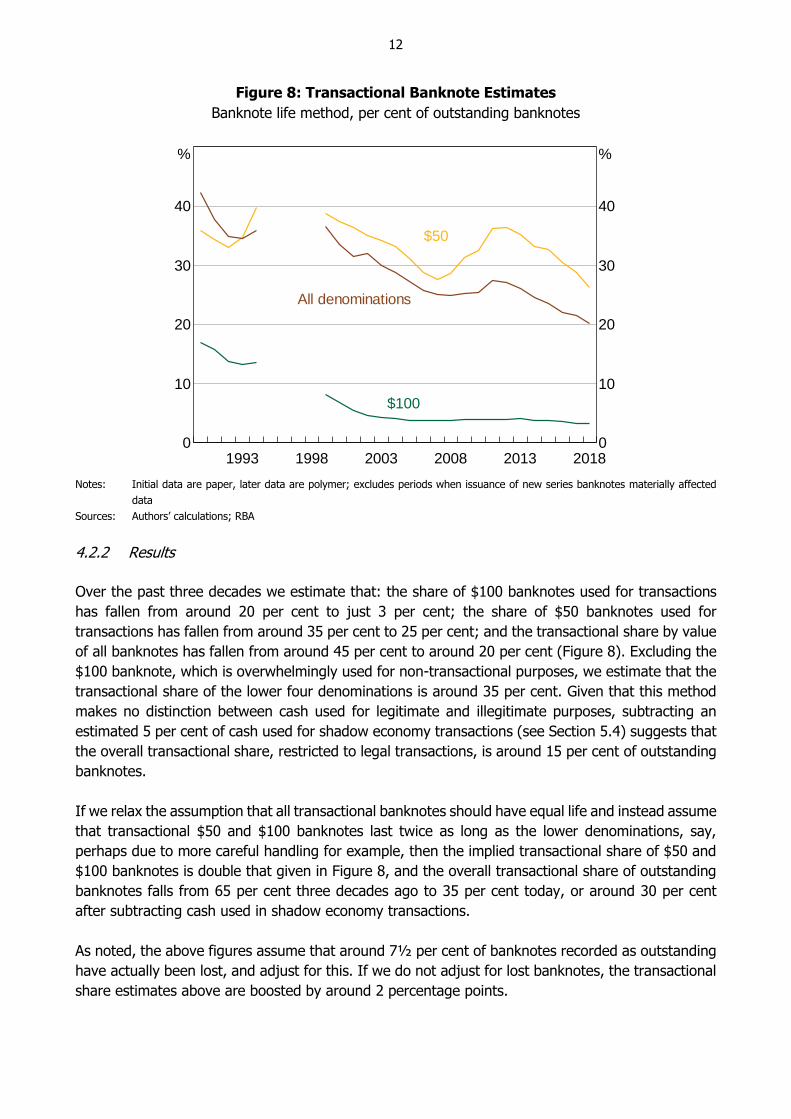
Figure 9 shows the average number of times each banknote denomination passes through a cash

depot per year, and a few features are worth observing. First, in recent years there has been a

general decline in the banknote processing frequencies of all denominations. This is consistent with

a fall in the velocity of cash and/or consumers substituting away from cash as a means of payment,

both of which result in banknotes passing through depots less frequently. Second, we see that the

$50 and $100 banknotes pass through depots less frequently than $20 banknotes, which is indicative

of non-transactional demand for these denominations given that, once spent, they are very likely to

be banked (retailers don’t keep $100 banknotes to use as change). Conversely, the low processing

frequency for the $5 and $10 banknotes is most likely due to their use as change – that is, they

cycle between consumers and retailers many times before being returned to a cash depot for

processing.

Figure 9: Banknote Processing Frequency

Average number of times processed over previous 12 months

Notes: Excludes periods when changes in banknote distribution arrangements materially affected the data; data either side of the

break are not directly comparable


Given these observations, we make two assumptions:

the non-transactional stock consists only of $50 and $100 banknotes;

20142010200620021998 20180

2

4

6

no

0

2

4

6

no

$100

$50

$10 $5

$20

14

the processing frequency of the transactional stock of $50 and $100 banknotes is equal to the

processing frequency of the $20 banknote.

These assumptions imply that non-transactional demand is the reason that the processing frequency

of $50 and $100 banknotes is less than for $20 banknotes, and allow us to estimate the extent of

hoarding of the higher denominations. As discussed in Section 4.2, the first assumption, while not

entirely true, is likely to be broadly accurate. The second assumption is somewhat more tenuous,

however, as the true processing frequency of the transactional stock of $50 and $100 banknotes is

likely to be higher than for the $20 as almost all $50 and $100 banknotes received by retailers are

likely to be banked, whereas some $20 banknotes will be given as change. This will result in an

upwardly-biased transactional share estimate.

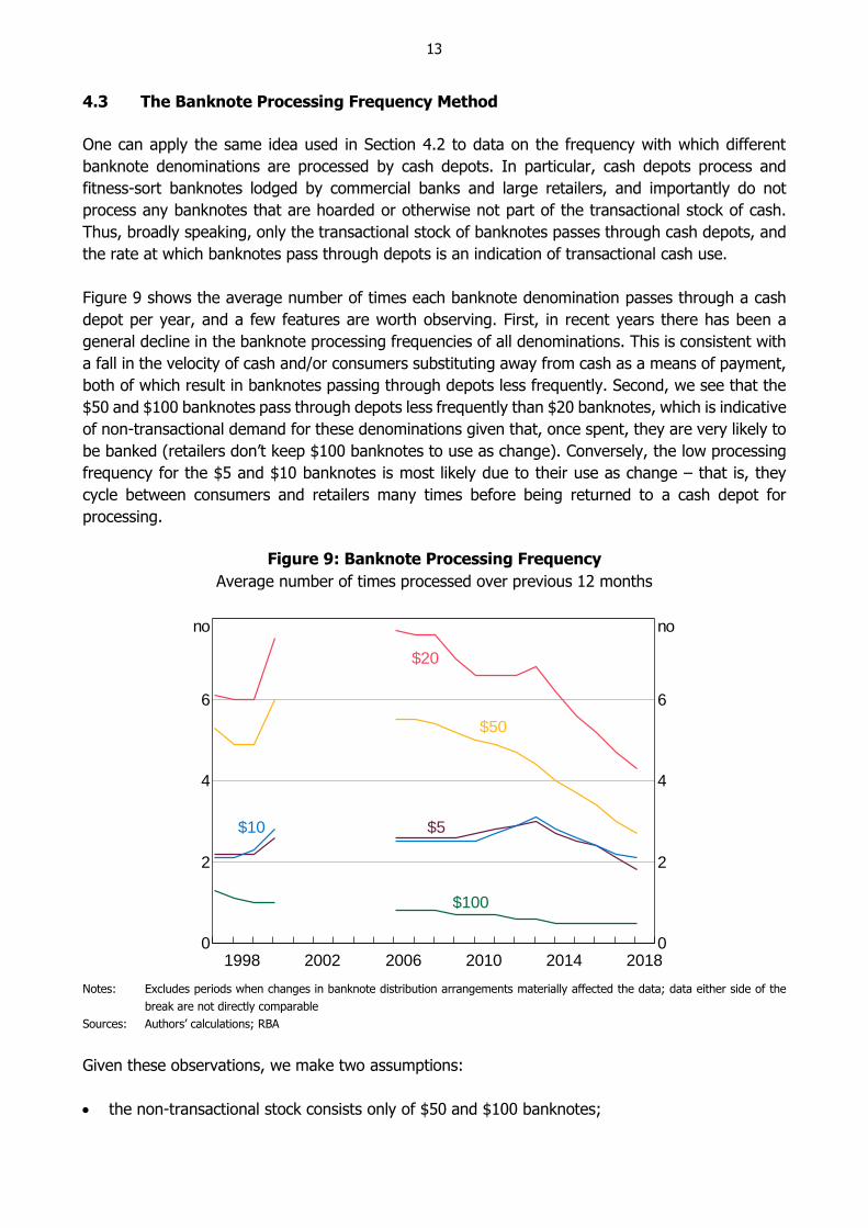
The results of this method suggest that the transactional stock has fallen from around 55 per cent

of total outstanding banknotes in the late 1990s to around 40 per cent now, or 35 per cent after

subtracting cash used in shadow economy transactions (Figure 10). As above, these figures adjust

for estimated lost banknotes; removing this adjustment boosts the estimated transactional share by

around 3 percentage points.


Banknote processing frequency method, per cent of outstanding banknotes

Note: Excludes periods when changes in banknote distribution arrangements materially affected the data


4.4 The Velocity Method

An important determinant of the stock of cash needed to facilitate transactional demand is the flow

of payments made using cash. However, the flow of cash payments does not, on its own, tell you

about the stock of cash used to facilitate transactions, as one banknote can be used in multiple

transactions over a period. To connect the flow of cash payments with the transactional stock, we

need to have an understanding of the velocity of cash: the average number of times the transactional

20142010200620021998 20180

20

40

60

80

%

0

20

40

60

80

%

$100

$50

All denominations

15

stock is used in a given period. For example, if the flow of total cash payments in a month was

$20 billion, and the transactional stock of cash was $10 billion, the entire stock must have turned

over twice in the month: velocity, in units per months, would be 2. This concept is summarised in

the following equation:

Flowof cash payments Velocityof transactional stock Valueof transactional stock

We now turn to estimating flow of cash payments and the velocity of transactional cash in order to

estimate the value of the transactional stock of cash.

4.4.1 The value of cash payments

Long-term determinants of cash payments include consumer payment preferences, accessibility of

alternative payment methods, and macroeconomic factors such as nominal consumer spending and

interest rates. Unlike card payments, however, the value of cash payments is not observed directly

and so must be estimated. To do so we distinguish between payments made using cash sourced

within Australia and cash sourced overseas. We estimate the value of cash payments made with

cash sourced in Australia by scaling card payment data collected by the Reserve Bank with the cash-

to-card payment ratio from the CPS.7 To approximate the value of cash payments made with cash

sourced from overseas, we subtract the value of card payments and ATM withdrawals made with

international cards from estimated total tourist spending obtained from Tourism Research Australia,

and also adjust for estimates of tourists’ domestically sourced income.8

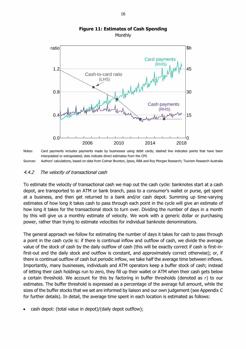
Applying this approach, Figure 11 shows estimated total cash payments increasing over the past

four years, after declining by approximately 40 per cent between 2007 and 2013. This stabilisation

and rebound is a function of consistent growth in total payments (due to factors such as population

and nominal income growth), combined with the cash-to-card ratio by value recorded in the 2016

CPS being little changed from 2013 (despite the ratio by number falling substantially). The earlier

sharp fall is driven by a steep decline in the cash-to-card ratio between 2010 and 2013.9

7 Respondents to the CPS record all payments made over a week and the method with which each payment was made,

allowing us to estimate the ratio of cash to card payments. We interpolate this ratio between survey years and

extrapolate the 2013–16 trend for 2017 and 2018. If we instead use ATM withdrawals as a proxy for cash spending

we obtain similar results.

8 Here we project tourist spending forward for the first six months of 2018 to fill in missing data; as this is only a small

component of total cash spending, any errors are unlikely to have a material impact.

9 The 2013 cash-to-card ratio appears to be somewhat of an anomaly, and from a visual inspection appears ‘too low’

when compared with the ratio in 2010 and 2016; if one adjusted the ratio up in line with the pattern displayed by the

other three readings, one would see a more gentle but sustained fall in estimated cash spending over the past decade.

The 2019 CPS should shed more light on the evolution of consumer payment preferences.

16

Figure 11: Estimates of Cash Spending

Monthly

Notes: Card payments includes payments made by businesses using debit cards; dashed line indicates points that have been

interpolated or extrapolated; dots indicate direct estimates from the CPS

Sources: Authors’ calculations, based on data from Colmar Brunton, Ipsos, RBA and Roy Morgan Research; Tourism Research Australia

4.4.2 The velocity of transactional cash

To estimate the velocity of transactional cash we map out the cash cycle: banknotes start at a cash

depot, are transported to an ATM or bank branch, pass to a consumer’s wallet or purse, get spent

at a business, and then get returned to a bank and/or cash depot. Summing up time-varying

estimates of how long it takes cash to pass through each point in the cycle will give an estimate of

how long it takes for the transactional stock to turn over. Dividing the number of days in a month

by this will give us a monthly estimate of velocity. We work with a generic dollar or purchasing

power, rather than trying to estimate velocities for individual banknote denominations.

The general approach we follow for estimating the number of days it takes for cash to pass through

a point in the cash cycle is: if there is continual inflow and outflow of cash, we divide the average

value of the stock of cash by the daily outflow of cash (this will be exactly correct if cash is first-in-

first-out and the daily stock and outflow is constant, and approximately correct otherwise); or, if

there is continual outflow of cash but periodic inflow, we take half the average time between inflows.

Importantly, many businesses, individuals and ATM operators keep a buffer stock of cash; instead

of letting their cash holdings run to zero, they fill up their wallet or ATM when their cash gets below

a certain threshold. We account for this by factoring in buffer thresholds (denoted as r) to our

estimates. The buffer threshold is expressed as a percentage of the average full amount, while the

sizes of the buffer stocks that we set are informed by liaison and our own judgement (see Appendix C

for further details). In detail, the average time spent in each location is estimated as follows:

cash depot: (total value in depot)/(daily depot outflow);

201420102006 20180.0

0.4

0.8

1.2

ratio

0

15

30

45

$b

Card payments(RHS)

Cash payments(RHS)

Cash-to-card ratio(LHS)

17

wallet: ((1 + 2r) × (days in month) ÷ (average number of cash withdrawals per person per

month)) ÷ 2; we divide by 2 to get an average time rather than the maximum time that a

banknote stays in someone’s wallet;

ATM: ((1+2r) × (days in month) ÷ (average number of ATM refills per month)) ÷ 2; the average

number of ATM refills per month is estimated using the total value of ATM withdrawals per

month, the total number of ATMs, and the effective capacity of the average ATM;

cash register or till: (1+2r) × (1 day estimated time spent in till).

Due to a lack of data we assume that cash flows through commercial bank branches take a similar

amount of time as flows through ATMs, and deviations from the assumption will bias our results. In

addition, we add in approximations of the time cash spends in transit between various holding points

(e.g. from a cash depot to an ATM, or from when cash is initially put into a retailer’s safe to when it

is subsequently deposited at a bank branch). We refer to this as the number of days cash spends in

transit. Finally, to estimate the velocity of overseas-sourced cash, we multiply the velocity of

domestically sourced cash by a scaling factor.

Given the inherent uncertainty involved in estimating the buffer stocks, the additional time taken for

overseas-sourced cash to circulate, and the time banknotes spend in transit, we present three

different scenarios. They are summarised in Table 2.

Table 2: Range of Velocity Assumptions

High velocity Medium velocity Low velocity

Wallet buffer 5 per cent of average

withdrawal

20 per cent of average

withdrawal

35 per cent of average

withdrawal

ATM buffer 5 per cent of capacity 15 per cent of capacity 25 per cent of capacity

Till buffer(a) $300 $500 $700

Overseas scaling factor 2 times slower than

domestic velocity

4 times slower than

domestic velocity

6 times slower than

domestic velocity

Transit time 3 working days 5 working days 7 working days

Note: (a) The buffer stock held in tills for the period studied is CPI-adjusted to be equivalent to the listed value in 2017

4.4.3 Results

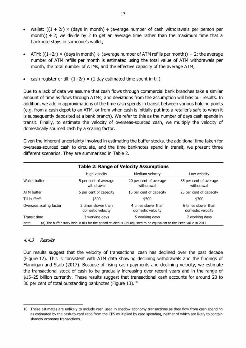
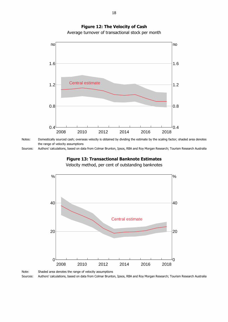
Our results suggest that the velocity of transactional cash has declined over the past decade

(Figure 12). This is consistent with ATM data showing declining withdrawals and the findings of

Flannigan and Staib (2017). Because of rising cash payments and declining velocity, we estimate

the transactional stock of cash to be gradually increasing over recent years and in the range of

$15–25 billion currently. These results suggest that transactional cash accounts for around 20 to

30 per cent of total outstanding banknotes (Figure 13).10

10 These estimates are unlikely to include cash used in shadow economy transactions as they flow from cash spending

as estimated by the cash-to-card ratio from the CPS multiplied by card spending, neither of which are likely to contain

shadow economy transactions.

18

Figure 12: The Velocity of Cash

Average turnover of transactional stock per month

Notes: Domestically sourced cash; overseas velocity is obtained by dividing the estimate by the scaling factor; shaded area denotes

the range of velocity assumptions



Velocity method, per cent of outstanding banknotes

Note: Shaded area denotes the range of velocity assumptions


20162014201220102008 20180.4

0.8

1.2

1.6

no

0.4

0.8

1.2

1.6

no

Central estimate

20162014201220102008 20180

20

40

%

0

20

40

%

Central estimate

19

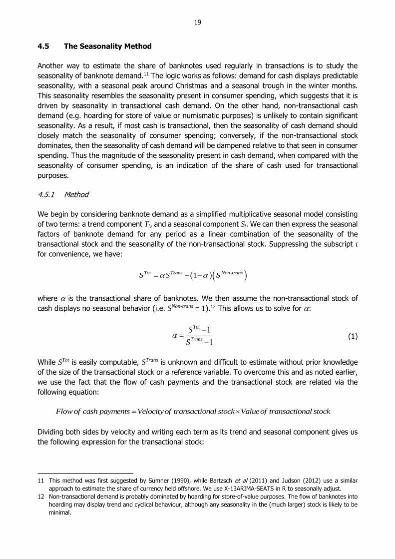
4.5 The Seasonality Method

Another way to estimate the share of banknotes used regularly in transactions is to study the

seasonality of banknote demand.11 The logic works as follows: demand for cash displays predictable

seasonality, with a seasonal peak around Christmas and a seasonal trough in the winter months.

This seasonality resembles the seasonality present in consumer spending, which suggests that it is

driven by seasonality in transactional cash demand. On the other hand, non-transactional cash

demand (e.g. hoarding for store of value or numismatic purposes) is unlikely to contain significant

seasonality. As a result, if most cash is transactional, then the seasonality of cash demand should

closely match the seasonality of consumer spending; conversely, if the non-transactional stock

dominates, then the seasonality of cash demand will be dampened relative to that seen in consumer

spending. Thus the magnitude of the seasonality present in cash demand, when compared with the

seasonality of consumer spending, is an indication of the share of cash used for transactional

purposes.

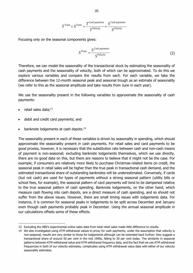
4.5.1 Method

We begin by considering banknote demand as a simplified multiplicative seasonal model consisting

of two terms: a trend component Tt, and a seasonal component St. We can then express the seasonal

factors of banknote demand for any period as a linear combination of the seasonality of the

transactional stock and the seasonality of the non-transactional stock. Suppressing the subscript t

for convenience, we have:

-1Tot Trans Non transS S S

where is the transactional share of banknotes. We then assume the non-transactional stock of

cash displays no seasonal behavior (i.e. SNon-trans = 1).12 This allows us to solve for :

1

1

Tot

Trans

S

S

(1)

While STot is easily computable, STrans is unknown and difficult to estimate without prior knowledge

of the size of the transactional stock or a reference variable. To overcome this and as noted earlier,

we use the fact that the flow of cash payments and the transactional stock are related via the

following equation:

Flowof cash payments Velocityof transactional stock Valueof transactional stock

Dividing both sides by velocity and writing each term as its trend and seasonal component gives us

the following expression for the transactional stock:

11 This method was first suggested by Sumner (1990), while Bartzsch et al (2011) and Judson (2012) use a similar

approach to estimate the share of currency held offshore. We use X-13ARIMA-SEATS in R to seasonally adjust.

12 Non-transactional demand is probably dominated by hoarding for store-of-value purposes. The flow of banknotes into

hoarding may display trend and cyclical behaviour, although any seasonality in the (much larger) stock is likely to be

minimal.

20

Cash payments Cash paymentsTrans Trans

Velocity Velocity

T ST S

T S

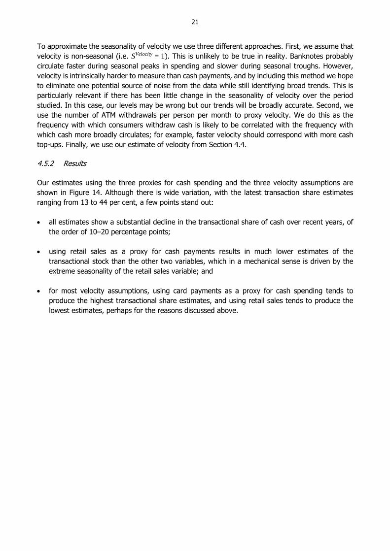
Focusing only on the seasonal components gives:

Cash paymentsTrans

Velocity

SS

S (2)

Therefore, we can model the seasonality of the transactional stock by estimating the seasonality of

cash payments and the seasonality of velocity, both of which can be approximated. To do this we

explore various variables and compare the results from each. For each variable, we take the

difference between the 12-month seasonal peak and seasonal trough as an estimate of seasonality

(we refer to this as the seasonal amplitude and take results from June in each year).

We use the seasonality present in the following variables to approximate the seasonality of cash

payments:

retail sales data;13

debit and credit card payments; and

banknote lodgements at cash depots.14

The seasonality present in each of these variables is driven by seasonality in spending, which should

approximate the seasonality present in cash payments. For retail sales and card payments to be

good proxies, however, it is necessary that the substitution rate between cash and non-cash means

of payment is non-seasonal; excluding banknote lodgements themselves, which we use directly,

there are no good data on this, but there are reasons to believe that it might not be the case. For

example, if consumers are relatively more likely to purchase Christmas-related items on credit, the

seasonal peak in retail sales will be higher than the true peak in transactional cash demand, and the

estimated transactional share of outstanding banknotes will be underestimated. Conversely, if cards

(but not cash) are used for types of payments without a strong seasonal pattern (utility bills or

school fees, for example), the seasonal pattern of card payments will tend to be dampened relative

to the true seasonal pattern of cash spending. Banknote lodgements, on the other hand, which

measure cash flowing into cash depots, are a direct measure of cash spending, and so should not

suffer from the above issues. However, there are small timing issues with lodgements data. For

instance, it is common for seasonal peaks in lodgements to be split across December and January

even though cash payments probably peak in December. Using the annual seasonal amplitude in

our calculations offsets some of these effects.

13 Excluding the ABS’s experimental online sales data from total retail sales made little difference to results.

14 We also investigated using ATM withdrawal values to proxy for cash payments; under the assumption that velocity is

non-seasonal, results are very similar to those for lodgements although can be extended back further; they suggest a

transactional share of around 50 per cent in the mid 1990s, falling to 30 per cent today. The similarity in seasonal

patterns between ATM withdrawal value and ATM withdrawal frequency data, and the fact that we use ATM withdrawal

frequencies in both of our velocity estimates, complicates using ATM withdrawal value data with either of our velocity

seasonality estimates.

21

To approximate the seasonality of velocity we use three different approaches. First, we assume that

velocity is non-seasonal (i.e. SVelocity = 1). This is unlikely to be true in reality. Banknotes probably

circulate faster during seasonal peaks in spending and slower during seasonal troughs. However,

velocity is intrinsically harder to measure than cash payments, and by including this method we hope

to eliminate one potential source of noise from the data while still identifying broad trends. This is

particularly relevant if there has been little change in the seasonality of velocity over the period

studied. In this case, our levels may be wrong but our trends will be broadly accurate. Second, we

use the number of ATM withdrawals per person per month to proxy velocity. We do this as the

frequency with which consumers withdraw cash is likely to be correlated with the frequency with

which cash more broadly circulates; for example, faster velocity should correspond with more cash

top-ups. Finally, we use our estimate of velocity from Section 4.4.

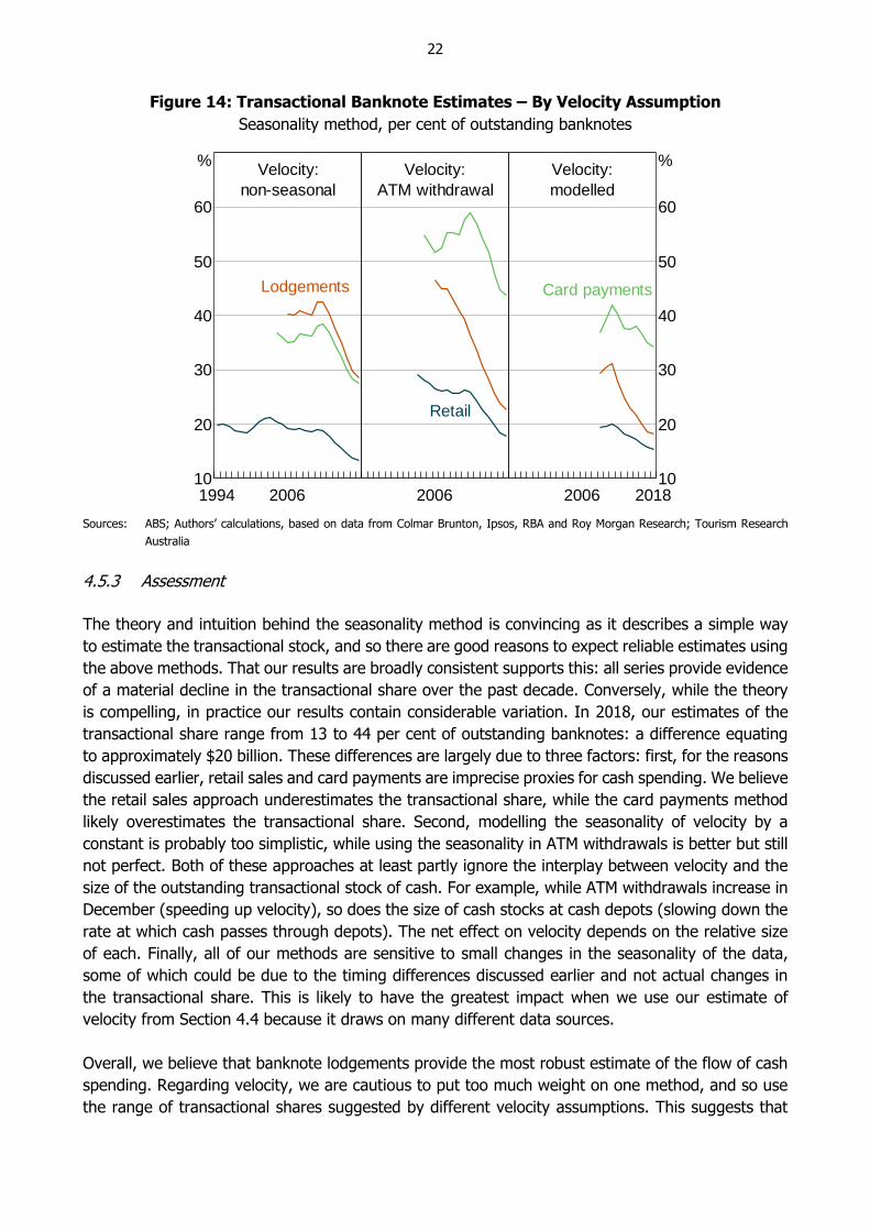
4.5.2 Results

Our estimates using the three proxies for cash spending and the three velocity assumptions are

shown in Figure 14. Although there is wide variation, with the latest transaction share estimates

ranging from 13 to 44 per cent, a few points stand out:

all estimates show a substantial decline in the transactional share of cash over recent years, of

the order of 10–20 percentage points;

using retail sales as a proxy for cash payments results in much lower estimates of the

transactional stock than the other two variables, which in a mechanical sense is driven by the

extreme seasonality of the retail sales variable; and

for most velocity assumptions, using card payments as a proxy for cash spending tends to

produce the highest transactional share estimates, and using retail sales tends to produce the

lowest estimates, perhaps for the reasons discussed above.

22

Figure 14: Transactional Banknote Estimates – By Velocity Assumption

Seasonality method, per cent of outstanding banknotes

Sources: ABS; Authors’ calculations, based on data from Colmar Brunton, Ipsos, RBA and Roy Morgan Research; Tourism Research

Australia

4.5.3 Assessment

The theory and intuition behind the seasonality method is convincing as it describes a simple way

to estimate the transactional stock, and so there are good reasons to expect reliable estimates using

the above methods. That our results are broadly consistent supports this: all series provide evidence

of a material decline in the transactional share over the past decade. Conversely, while the theory

is compelling, in practice our results contain considerable variation. In 2018, our estimates of the

transactional share range from 13 to 44 per cent of outstanding banknotes: a difference equating

to approximately $20 billion. These differences are largely due to three factors: first, for the reasons

discussed earlier, retail sales and card payments are imprecise proxies for cash spending. We believe

the retail sales approach underestimates the transactional share, while the card payments method

likely overestimates the transactional share. Second, modelling the seasonality of velocity by a

constant is probably too simplistic, while using the seasonality in ATM withdrawals is better but still

not perfect. Both of these approaches at least partly ignore the interplay between velocity and the

size of the outstanding transactional stock of cash. For example, while ATM withdrawals increase in

December (speeding up velocity), so does the size of cash stocks at cash depots (slowing down the

rate at which cash passes through depots). The net effect on velocity depends on the relative size

of each. Finally, all of our methods are sensitive to small changes in the seasonality of the data,

some of which could be due to the timing differences discussed earlier and not actual changes in

the transactional share. This is likely to have the greatest impact when we use our estimate of

velocity from Section 4.4 because it draws on many different data sources.

Overall, we believe that banknote lodgements provide the most robust estimate of the flow of cash

spending. Regarding velocity, we are cautious to put too much weight on one method, and so use

the range of transactional shares suggested by different velocity assumptions. This suggests that

Velocity:

non-seasonal

2006199410

20

30

40

50

60

%

Lodgements

Velocity:

ATM withdrawal

2006

Retail

Velocity:

modelled

2006 201810

20

30

40

50

60

%

Card payments

23

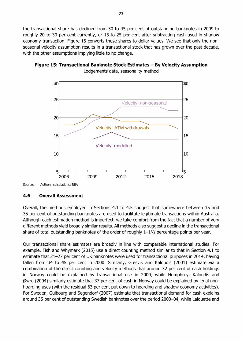
the transactional share has declined from 30 to 45 per cent of outstanding banknotes in 2009 to

roughly 20 to 30 per cent currently, or 15 to 25 per cent after subtracting cash used in shadow

economy transaction. Figure 15 converts these shares to dollar values. We see that only the non-

seasonal velocity assumption results in a transactional stock that has grown over the past decade,

with the other assumptions implying little to no change.

Figure 15: Transactional Banknote Stock Estimates – By Velocity Assumption

Lodgements data, seasonality method


4.6 Overall Assessment

Overall, the methods employed in Sections 4.1 to 4.5 suggest that somewhere between 15 and

35 per cent of outstanding banknotes are used to facilitate legitimate transactions within Australia.

Although each estimation method is imperfect, we take comfort from the fact that a number of very

different methods yield broadly similar results. All methods also suggest a decline in the transactional

share of total outstanding banknotes of the order of roughly 1–1½ percentage points per year.

Our transactional share estimates are broadly in line with comparable international studies. For

example, Fish and Whymark (2015) use a direct counting method similar to that in Section 4.1 to

estimate that 21–27 per cent of UK banknotes were used for transactional purposes in 2014, having

fallen from 34 to 45 per cent in 2000. Similarly, Gresvik and Kaloudis (2001) estimate via a

combination of the direct counting and velocity methods that around 32 per cent of cash holdings

in Norway could be explained by transactional use in 2000, while Humphrey, Kaloudis and

Øwre (2004) similarly estimate that 37 per cent of cash in Norway could be explained by legal non-

hoarding uses (with the residual 63 per cent put down to hoarding and shadow economy activities).

For Sweden, Guibourg and Segendorf (2007) estimate that transactional demand for cash explains

around 35 per cent of outstanding Swedish banknotes over the period 2000–04, while Lalouette and

2015201220092006 20185

10

15

20

25

$b

5

10

15

20

25

$b

Velocity: non-seasonal

Velocity: modelled

Velocity: ATM withdrawals

24

Esselink (2018) use a processing frequency method to estimate that around one-quarter of euro

banknotes are used for transactional purposes within the euro area.15

A number of studies use econometric models to indirectly estimate the flow or stock of transactional

cash demand. For example, Snellman, Vesala and Humphrey (2001) regress growth in card

payments on growth in outstanding currency and growth in GDP, and then use the estimated

coefficients to back-out the implied flow demand for transactional cash, controlling for the number

of ATM and EFTPOS terminals per person. Seitz (2007) postulates that the stock of transactional

cash balances (plus overnight deposits) determines inflation, and estimates the share of cash used

for transactions as that which leads to the best-fitting inflation equation. We do not follow these

approaches as the assumptions needed to generate results seem unrealistic (in the two examples

given, that changing preferences between cash and electronic payment methods over time can be

captured by the number of ATM and EFTPOS terminals, and that physical banknote holdings are a

major determinant of inflation, respectively), while a more robust method to estimate the flow of

transactional cash demand is open to us as discussed in Section 4.4.

5. The Shadow Economy

A source of currency demand that continues to attract considerable attention in Australia and

internationally is the use of cash to facilitate illicit activities in the ‘shadow’ or ‘black’ economy.

Borrowing from ABS (2013) we define the shadow economy as consisting of:

underground production (deliberate concealment of legal activities to avoid tax payments); and

illegal production (activities forbidden by law where there is mutual consent, such as illegal drug

production and sale).

The System of National Accounts 2008 also includes informal production (the production of goods

or services with the primary objective of generating employment and incomes to the persons

concerned), household production for own final use (includes production of crops, livestock,

construction of own houses, imputed rents, and domestic services) and the statistical underground

(production missed by statistical agencies due to deficiencies in data collection) as part of the non-

observed economy. But according to ABS (2013), informal production is not believed to be material

in Australia, while the latter two categories are unlikely to involve cash transactions and are not

considered here.

To estimate the stock of cash used in the shadow economy we must first have an idea about the

size of the shadow economy. By its very nature, the shadow economy is difficult to measure. To

ensure that our results are as robust as possible we use multiple sources to estimate its overall size,

including data from the ABS, the Black Economy Taskforce (BETF), and the Australian Criminal

15 Lalouette and Esselink also use the speed with which new series ES2 banknotes displaced old series ES1 banknotes

to estimate the degree of transactional demand in the euro area, with this method suggesting that 20 per cent of

outstanding euro banknotes are used for transactional purposes. We have comparable data – the speed with which

new series NGB $5 and $10 banknotes have displaced the old series $5 and $10 banknotes – but we do not pursue

this method as it implicitly assumes that i) any hoarded old series banknotes are not returned for new series banknotes,

and ii) that, after a certain date, all outstanding non-returned old series banknotes are hoarded. Neither assumption

seems robust.

25

Intelligence Commission (ACIC). We assume that the only material component of illegal production

is illegal drug production; this may downwardly bias our estimates slightly, although illegal drug

production is likely to be the largest component of total illegal production by some margin (the ABS

also took this approach when estimating illegal production in 2009/10).

5.1 ABS Estimates for 2009/10 Applied to 2017/18 GDP Figures

In 2013, the ABS estimated the size of the shadow economy for 2009/10. In particular, underground

production was estimated to be 1.5 per cent of nominal GDP in 2009/10, while household final

consumption expenditure (HFCE) on illegal drugs was estimated to be 0.8 per cent of total HFCE in

2009/10. Nominal GDP in 2017/18 was $1,848 billion, while HFCE in 2017/18 was $1,044 billion;

applying the same 1.5 and 0.8 per cent estimates as for 2009/10 implies annual underground

production of $27½ billion and annual nominal spending on illegal drugs of $8½ billion. We will

make the assumption that all these transactions are conducted using cash, although in practice it is

likely that a growing share are electronic.

To approximate the quantity of cash required to facilitate shadow economy activities, we have to

take into account that a single banknote can make multiple payments. To do so we divide total

spending by the estimated average number of times the stock of cash is used in a period, that is,

velocity. In Section 4.4 we compiled data from the cash cycle to estimate the monthly velocity of

the domestically sourced transactional stock of cash. The input variables included data from ATM

operators, banks and cash depots. It seems reasonable to assume that when a user sources cash to

purchase illicit drugs or pay for underground production, they do so in much the same way as when

they source cash for other reasons. Accordingly, we use our previous estimates of velocity as an

approximation of the velocity of cash used in the shadow economy. These estimates imply that

$2½ billion of cash, or around 3 per cent of the value of banknotes on issue, is used to facilitate

underground production, and that a little less than $1 billion of cash, or just under 1 per cent of the

value of banknotes on issue, is used to facilitate illegal production and purchase illicit drugs. That is,

we estimate the stock of cash used to facilitate shadow economy transactions to be around

$3½ billion, or 4 per cent of banknotes on issue.

5.2 Black Economy Taskforce Estimates

Building on the work of the ABS, the BETF recently provided partial estimates of the size of the

shadow economy.16 Their assessment was that the size of the shadow economy is up to 50 per cent

larger than that suggested by the ABS estimates, with the difference in part explained by the BETF

including a wider range of shadow economy activities in their analysis (some of which are unlikely

to involve material amounts of cash).

Boosting the estimates from Section 5.1 by 50 per cent suggests underground production of around

$41½ billion in 2017/18 and illegal production of roughly $12½ billion. Once again, if we assume

that all of these transactions were made with cash (likely incorrect) and adjust for the velocity of

cash, this implies that around $5 billion of cash, or around 7 per cent of the value of banknotes on

16 The BETF used the ABS estimates discussed above as a benchmark, but updated results where additional or enhanced

information had since become available.

26

issue, is used to facilitate shadow economy activities, with three-quarters used in underground

production and one-quarter in illegal production.

5.3 New Estimates of Cash Used in the Drug Trade

5.3.1 Estimates of cash used to purchase illicit drugs

Here we estimate spending on illicit drugs via wastewater analysis. Wastewater analysis is a standard

method used to measure drug consumption. The method is based on ‘the principle that any given

compound that is consumed … will subsequently be excreted’ (ACIC 2018b, p 17) and end up in the

sewer system. Calculating the amount of a given compound in wastewater allows for a back

calculation factor to be applied to determine the amount of drug that was used by the population

connected to the wastewater. National estimates of annual drug consumption are then made by

scaling the results to population levels.

ACIC, in conjunction with the University of Queensland and the University of South Australia,

performs wastewater analysis at more than 40 sites across Australia each year, covering

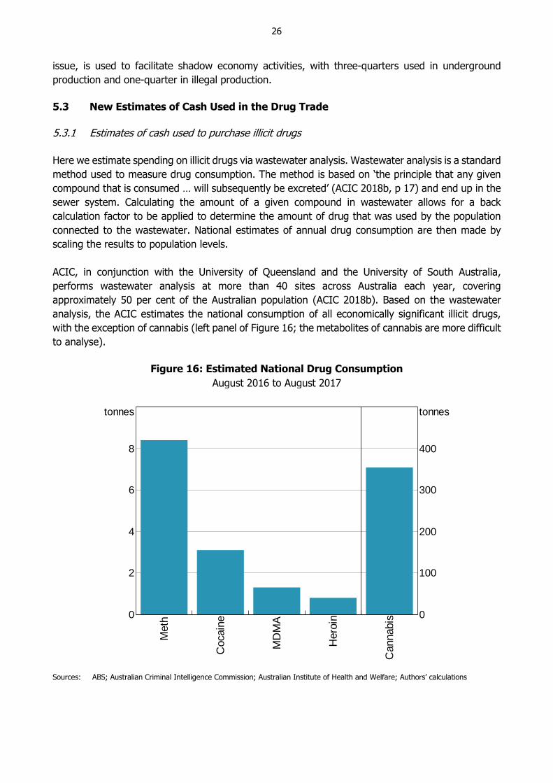
approximately 50 per cent of the Australian population (ACIC 2018b). Based on the wastewater

analysis, the ACIC estimates the national consumption of all economically significant illicit drugs,

with the exception of cannabis (left panel of Figure 16; the metabolites of cannabis are more difficult

to analyse).

Figure 16: Estimated National Drug Consumption

August 2016 to August 2017

Sources: ABS; Australian Criminal Intelligence Commission; Australian Institute of Health and Welfare; Authors’ calculations

Meth

Cocain

e

MD

MA

Hero

in

Cannabis0

2

4

6

8

tonnes

0

100

200

300

400

tonnes

27

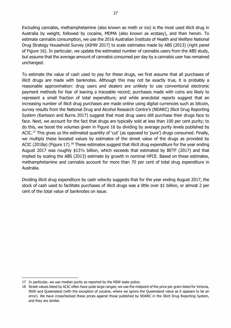
Excluding cannabis, methamphetamine (also known as meth or ice) is the most used illicit drug in

Australia by weight, followed by cocaine, MDMA (also known as ecstasy), and then heroin. To

estimate cannabis consumption, we use the 2016 Australian Institute of Health and Welfare National

Drug Strategy Household Survey (AIHW 2017) to scale estimates made by ABS (2013) (right panel

of Figure 16). In particular, we update the estimated number of cannabis users from the ABS study,

but assume that the average amount of cannabis consumed per day by a cannabis user has remained

unchanged.

To estimate the value of cash used to pay for these drugs, we first assume that all purchases of

illicit drugs are made with banknotes. Although this may not be exactly true, it is probably a

reasonable approximation: drug users and dealers are unlikely to use conventional electronic

payment methods for fear of leaving a traceable record; purchases made with coins are likely to

represent a small fraction of total expenditure; and while anecdotal reports suggest that an

increasing number of illicit drug purchases are made online using digital currencies such as bitcoin,

survey results from the National Drug and Alcohol Research Centre’s (NDARC) Illicit Drug Reporting

System (Karlsson and Burns 2017) suggest that most drug users still purchase their drugs face to

face. Next, we account for the fact that drugs are typically sold at less than 100 per cent purity; to

do this, we boost the volumes given in Figure 16 by dividing by average purity levels published by

ACIC.17 This gives us the estimated quantity of ‘cut’ (as opposed to ‘pure’) drugs consumed. Finally,

we multiply these boosted values by estimates of the street value of the drugs as provided by

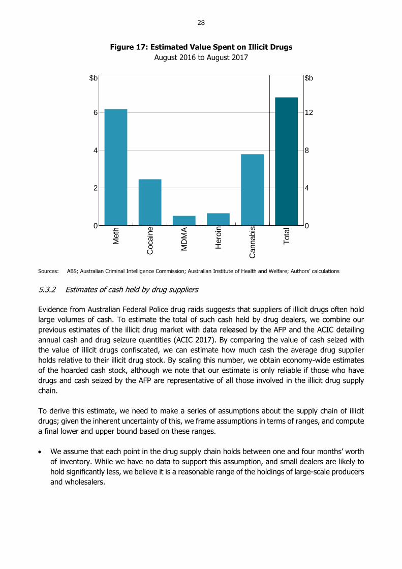
ACIC (2018a) (Figure 17).18 These estimates suggest that illicit drug expenditure for the year ending

August 2017 was roughly $13½ billion, which exceeds that estimated by BETF (2017) and that

implied by scaling the ABS (2013) estimate by growth in nominal HFCE. Based on these estimates,

methamphetamine and cannabis account for more than 70 per cent of total drug expenditure in

Australia.

Dividing illicit drug expenditure by cash velocity suggests that for the year ending August 2017, the

stock of cash used to facilitate purchases of illicit drugs was a little over $1 billion, or almost 2 per

cent of the total value of banknotes on issue.

17 In particular, we use median purity as reported by the NSW state police.

18 Street values listed by ACIC often have quite large ranges; we use the midpoint of the price per gram listed for Victoria,

NSW and Queensland (with the exception of cocaine, where we ignore the Queensland value as it appears to be an

error). We have crosschecked these prices against those published by NDARC in the Illicit Drug Reporting System,

and they are similar.

https://www.acic.gov.au/sites/g/files/net1491/f/2017/06/illicit_drug_data_report_2015-16_full_report.pdf?v=1498019727

https://www.acic.gov.au/sites/g/files/net1491/f/2017/06/illicit_drug_data_report_2015-16_full_report.pdf?v=1498019727

28

Figure 17: Estimated Value Spent on Illicit Drugs

August 2016 to August 2017

Sources: ABS; Australian Criminal Intelligence Commission; Australian Institute of Health and Welfare; Authors’ calculations

5.3.2 Estimates of cash held by drug suppliers

Evidence from Australian Federal Police drug raids suggests that suppliers of illicit drugs often hold

large volumes of cash. To estimate the total of such cash held by drug dealers, we combine our

previous estimates of the illicit drug market with data released by the AFP and the ACIC detailing

annual cash and drug seizure quantities (ACIC 2017). By comparing the value of cash seized with

the value of illicit drugs confiscated, we can estimate how much cash the average drug supplier

holds relative to their illicit drug stock. By scaling this number, we obtain economy-wide estimates

of the hoarded cash stock, although we note that our estimate is only reliable if those who have

drugs and cash seized by the AFP are representative of all those involved in the illicit drug supply

chain.

To derive this estimate, we need to make a series of assumptions about the supply chain of illicit

drugs; given the inherent uncertainty of this, we frame assumptions in terms of ranges, and compute

a final lower and upper bound based on these ranges.

We assume that each point in the drug supply chain holds between one and four months’ worth

of inventory. While we have no data to support this assumption, and small dealers are likely to

hold significantly less, we believe it is a reasonable range of the holdings of large-scale producers

and wholesalers.

Meth

Cocain

e

MD

MA

Hero

in

Cannabis

Tota

l0

2

4

6

$b

0

4

8

12

$b

https://acic.govcms.gov.au/sites/g/files/net1491/f/acic_2016-17_annual_report.pdf?v=1508387578

29

We assume that the illicit drug supply chain contains between two and four layers, with each

layer holding a similar ratio of cash to drugs.

We assume that the ratio of total attempted drug supply to total drug consumption is between

1 and 3 times (that is, for every gram of drug consumed, up to 2 grams of the same drug is lost

or seized by police). Accounting for ‘spoilage’ is necessary as a significant portion of illicit drugs

are removed from the supply chain prior to consumption. For example, the ACIC estimates that

in 2016/17 the total weight of cocaine seized exceeded annual national consumption, while the

total weight of MDMA seized was roughly equal to annual national consumption.

Data from cash and drug seizures suggest that drug suppliers maintain cash holdings of around

2 per cent of the value of their stock of drugs, on average.19 By comparison, the same data suggest

that the proceeds of crime (that is, all assets gained through crime, not just cash) equate to

approximately 11 per cent of the value of the stock of drugs held. This implies that criminals convert

a large share of their cash profits into other assets: they do not solely hoard cash. Combining this

with our earlier assumptions suggests that total cash hoarding by the illicit drug supply chain is in

the range of $40 million to $1 billion, or somewhere between 0 and 1 per cent of all banknotes on

issue.

5.4 Overall Assessment and International Comparison

Our estimates suggest that between roughly $3½ and $6 billion worth of Australian banknotes are

used in the shadow economy, split between underground production ($2½–4 billion), purchases of

illegal drugs (around $1 billion), and storing the profits of criminal activity (up to $1 billion). This

represents between 4 and 8 per cent of all banknotes on issue, with the midpoint of the non-hoarded

‘transactional’ portion equating to around 5 per cent of banknotes on issue.

There exists a branch of literature which estimates shadow economy cash demand by assuming that

all growth in outstanding banknotes, from some initial date and above some baseline growth rate

(perhaps accounting for population growth and inflation, for example), is driven by shadow economy

activity; see, for example, Pickhardt and Sardà (2012) and the references therein for a thorough

overview. We do not pursue these techniques, however, as the assumptions needed to generate

results seem overly strong (studies often assume, for example, that no legitimate cash hoarding

exists, whereas we believe that legal cash hoarding likely accounts for much of the outstanding stock

of banknotes).

More broadly, estimates exist for many countries on the size of their shadow economies, and these

estimates are likely to be reasonable indicators of the stock of cash used in shadow economy activity.

Notably, in 2012 the OECD asked a range of countries to estimate the size of their shadow economy

using a set of guidelines (see OECD et al (2002) and Gyomai and van de Ven (2014)). Although

Australia was not included in the study, the ABS followed the same guidelines in ABS (2013). As a

share of GDP, the Australian shadow economy estimate was similar to that for Canada, the

Netherlands and the United Kingdom, which were all between roughly 1 and 3 per cent of GDP; this

19 In particular, over the five years to 2016/17, the ACIC reports total drug seizures worth $6.1 billion and total cash

seizures of $100 million (ACIC 2017).

https://acic.govcms.gov.au/sites/g/files/net3726/f/nwdmp4.pdf?v=1522809564

30

was below Sweden, Belgium and France for example (roughly 3 to 6 per cent of GDP), and far below

Italy (18 per cent of GDP). Some studies estimate much larger shadow economies, in the order of

15 per cent of GDP for Australia (e.g. Schneider, Buehn and Montenegro 2010; Medina and

Schneider 2018); we do not have the expertise to comment on the accuracy of these studies, but

refer the interested reader to the annex of Gyomai and van de Ven (2014) for a critique of the

methods employed, and also note the ABS’s assessment that ‘estimates of the order of 15% of GDP

for the underground economy are implausible’ (ABS 2013).

Regarding the denomination of banknotes used in illegal activities, although there is no hard data,

law enforcement agencies have suggested that $50 banknotes seem to dominate. This is anecdotally

supported by images of cash seizures released by police, which typically show bundles of $50

banknotes as the predominant denomination, together with lesser amounts of $20 and $100

banknotes.

6. Hoarding

The final component of currency demand that we examine is hoarding, which can be done either by

Australian residents (domestic hoarding) or by foreigners (international hoarding). Hoarding refers

to banknotes actively held by people for reasons other than to finance everyday payments, and so

excludes the transactional stock of banknotes (both legitimate and shadow economy), and

banknotes that have been lost. Evidence from the 2016 CPS suggests that approximately 70 per

cent of Australians hold cash outside of their wallets, and that they do so for a variety of reasons

including as a store of wealth, for use in emergencies, a desire for privacy, and as a backup in case

of problems with electronic payments systems (Figure 18).20 The existence of asset means-testing

for various social benefits in Australia, and more generally the desire to hide assets from tax

authorities, also provides an incentive for Australians to hold assets in a form that is hard to trace.

We now turn to estimating the level of hoarding using a variety of different methods.

20 For example, the Red Cross lists ‘extra cash’ as a minimum requirement of a survival kit for use in an emergency or

disaster scenario; available at <https://www.redcross.org/get-help/how-to-prepare-for-emergencies/survival-kit-

supplies.html>.

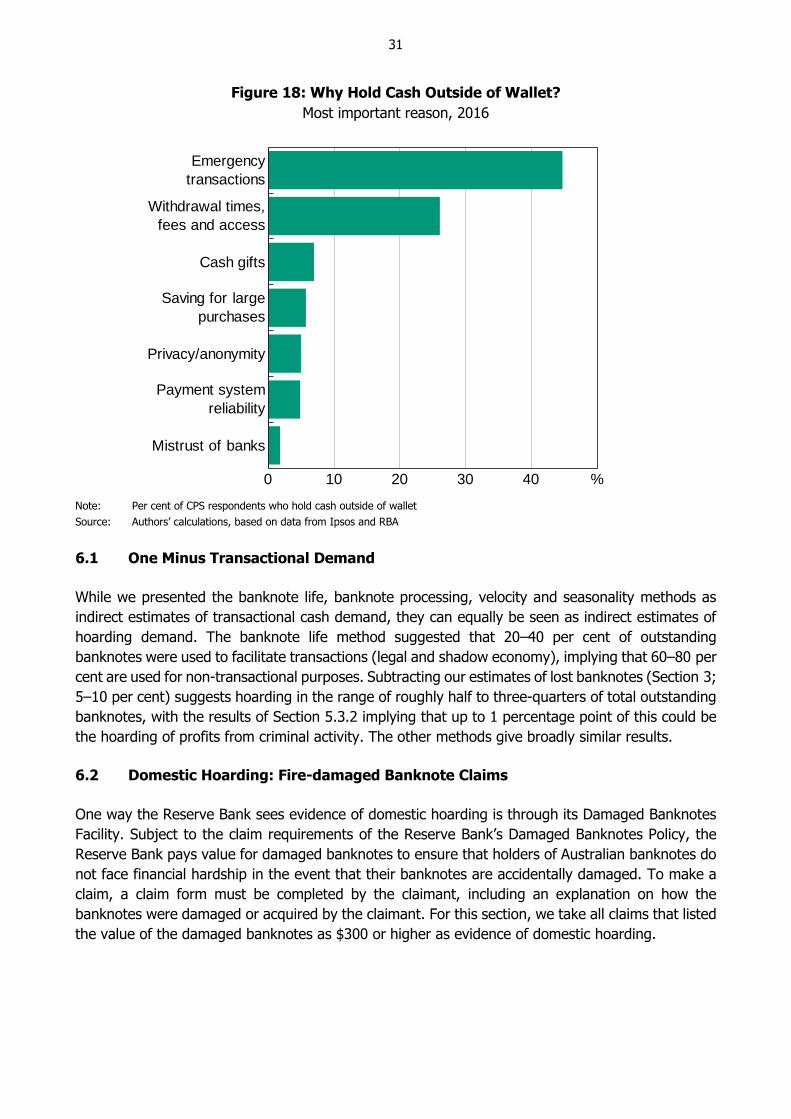
31

Figure 18: Why Hold Cash Outside of Wallet?

Most important reason, 2016

Note: Per cent of CPS respondents who hold cash outside of wallet

Source: Authors’ calculations, based on data from Ipsos and RBA

6.1 One Minus Transactional Demand

While we presented the banknote life, banknote processing, velocity and seasonality methods as

indirect estimates of transactional cash demand, they can equally be seen as indirect estimates of

hoarding demand. The banknote life method suggested that 20–40 per cent of outstanding

banknotes were used to facilitate transactions (legal and shadow economy), implying that 60–80 per

cent are used for non-transactional purposes. Subtracting our estimates of lost banknotes (Section 3;

5–10 per cent) suggests hoarding in the range of roughly half to three-quarters of total outstanding

banknotes, with the results of Section 5.3.2 implying that up to 1 percentage point of this could be

the hoarding of profits from criminal activity. The other methods give broadly similar results.

6.2 Domestic Hoarding: Fire-damaged Banknote Claims

One way the Reserve Bank sees evidence of domestic hoarding is through its Damaged Banknotes

Facility. Subject to the claim requirements of the Reserve Bank’s Damaged Banknotes Policy, the

Reserve Bank pays value for damaged banknotes to ensure that holders of Australian banknotes do

not face financial hardship in the event that their banknotes are accidentally damaged. To make a

claim, a claim form must be completed by the claimant, including an explanation on how the

banknotes were damaged or acquired by the claimant. For this section, we take all claims that listed

the value of the damaged banknotes as $300 or higher as evidence of domestic hoarding.

0 10 20 30 40 %

Mistrust of banks

Payment system

reliability

Privacy/anonymity

Saving for large

purchases

Cash gifts

Withdrawal times,

fees and access

Emergency

transactions

32

To estimate total domestic hoarding we make use of data on the number of uncontained residential

fires that spread beyond the object or room of origin.21 In particular, we make the following

assumptions (we discuss the validity of these after presenting our estimates):

all fire-affected households that hoarded banknotes lost those banknotes in the fire, made claims

to the Reserve Bank for their full value, and listed ‘fire damage’ as the cause of damage;

households affected by fires are representative of all Australian households; and

residential fires are random and unpredictable.

We can then estimate average household banknote hoarding using the following equation:

-

-

Value of fire damaged claimsAveragehousehold hoarding

No of fire affected households

Scaling this by the number of households in Australia gives an estimate of total domestic hoarding.

6.2.1 Results

For each fire-damaged banknote claim, two values are recorded: the value of banknotes the

claimants stated were destroyed, and the value paid by the Reserve Bank after assessment. Taking

these as upper and lower bounds, data for the four years to 2017/18 suggest that Australian

households hoard between 2 and 3 per cent of banknotes on issue, or approximately $60 to $90 per

Australian on average. By value, claims are roughly evenly split between $50 and $100

denominations, with relatively few claims for other denominations.

However, our estimates are only reliable if our assumptions are reasonable, which we believe is

probably not the case. This likely causes us to underestimate total cash hoarding. We briefly highlight

some of the key issues.

Fire-affected households are unlikely to be representative of the population, with factors such as

the wealth and occupation of the inhabitants of the dwelling, as well as the geographic location,

likely to influence the probability of a fire.

Related to this, if wealthier households are more likely to hoard cash, then the probability of

suffering a fire may be negatively related to the probability of hoarding cash: wealthier

households are arguably less likely to be fire-affected because their homes are more likely to be

built out of modern materials, have working fire alarms, and be located in cities near emergency

services. This will lead us to underestimate hoarding. Conversely, if wealthier households are less

likely to hoard cash, then by the previous argument, our estimates may contain some upward

bias.

21 Data available from <https://www.pc.gov.au/research/ongoing/report-on-government-services/2018/emergency-

management/emergency-services>.

33

Cash hoarding may also directly influence the likelihood of a fire: households that store large

sums of cash may invest relatively more in fire prevention methods to protect their cash holdings,

again leading to underestimates of hoarding.

Fire-damaged banknote claims may underestimate cash holdings of fire-affected houses. This will

occur when stored banknotes survive a fire or when households fail to make a claim to the

Reserve Bank (perhaps because they claim via their home insurance instead, or do not know

about the Reserve Bank’s policy on damaged banknotes).

6.3 Domestic Hoarding: Results from the Consumer Payments Survey

Another sample available to us is the Reserve Bank’s Consumer Payments Survey. In 2013 and 2016,

survey respondents were asked to select a range that described the amount of cash they held outside

their wallets. Scaling these results to economy-wide levels, we estimate that domestic cash hoarding

is in the range of roughly 10 to 20 per cent of total outstanding banknotes.22 Although this estimate

exceeds that made using damaged banknote claims, we believe it is likely still an underestimate, as

those with large physical cash holdings may be less likely to participate in a survey, and, even if they

do, might be hesitant to respond with the true extent of their holdings. More generally, the

distribution of hoarded cash is likely to have a long right tail, which makes accurately estimating the

extent of hoarding using a relatively small sample difficult.

6.4 International Hoarding: Outflow Less Inflow

The Reserve Bank has previously noted that overseas demand for Australian banknotes is an

increasingly important component of overall currency demand (Flannigan and Parsons 2018). This

is highlighted by a historically strong relationship between the exchange rate and demand for

$100 banknotes; depreciations in the Australian dollar are associated with an increase in demand,

although the relationship appears to have weakened somewhat of late (Figure 19). While much of

this demand is likely the result of foreign tourists obtaining Australian currency before arriving in

Australia, and subsequently spending the cash in Australia, some may be hoarded abroad indefinitely

for store of value and wealth diversification purposes.

22 The CPS asks respondents to select a bucket that their cash holdings fall into, from ‘$1–$100’ through to ‘more than

$5,000’. We take the midpoint of each value bucket, or $10,000 for the top, open-ended, bucket, as the average

hoarding of each respondent within each bucket, and scale up the results to be representative of the adult population.

For those who did not answer (2013 and 2016 surveys) or chose ‘prefer not to answer’ (2016 survey only), we set

their cash hoarding as the weighted average of those who did answer. For 2013 we estimate cash hoarding of 20 per

cent of outstanding banknotes, while for 2016 the estimate is lower at roughly 10 per cent, indicating that a large

degree of sampling error exists in these estimates.

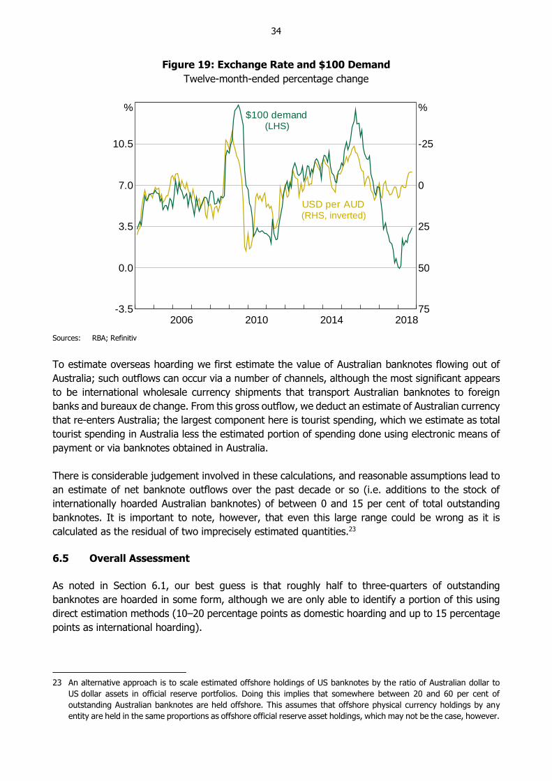
34

Figure 19: Exchange Rate and $100 Demand

Twelve-month-ended percentage change

Sources: RBA; Refinitiv

To estimate overseas hoarding we first estimate the value of Australian banknotes flowing out of

Australia; such outflows can occur via a number of channels, although the most significant appears

to be international wholesale currency shipments that transport Australian banknotes to foreign

banks and bureaux de change. From this gross outflow, we deduct an estimate of Australian currency

that re-enters Australia; the largest component here is tourist spending, which we estimate as total

tourist spending in Australia less the estimated portion of spending done using electronic means of

payment or via banknotes obtained in Australia.

There is considerable judgement involved in these calculations, and reasonable assumptions lead to

an estimate of net banknote outflows over the past decade or so (i.e. additions to the stock of

internationally hoarded Australian banknotes) of between 0 and 15 per cent of total outstanding

banknotes. It is important to note, however, that even this large range could be wrong as it is

calculated as the residual of two imprecisely estimated quantities.23

6.5 Overall Assessment

As noted in Section 6.1, our best guess is that roughly half to three-quarters of outstanding

banknotes are hoarded in some form, although we are only able to identify a portion of this using

direct estimation methods (10–20 percentage points as domestic hoarding and up to 15 percentage

points as international hoarding).

23 An alternative approach is to scale estimated offshore holdings of US banknotes by the ratio of Australian dollar to

US dollar assets in official reserve portfolios. Doing this implies that somewhere between 20 and 60 per cent of

outstanding Australian banknotes are held offshore. This assumes that offshore physical currency holdings by any

entity are held in the same proportions as offshore official reserve asset holdings, which may not be the case, however.

201420102006 2018-3.5

0.0

3.5

7.0

10.5

%

75

50

25

0

-25

%$100 demand

(LHS)

USD per AUD(RHS, inverted)

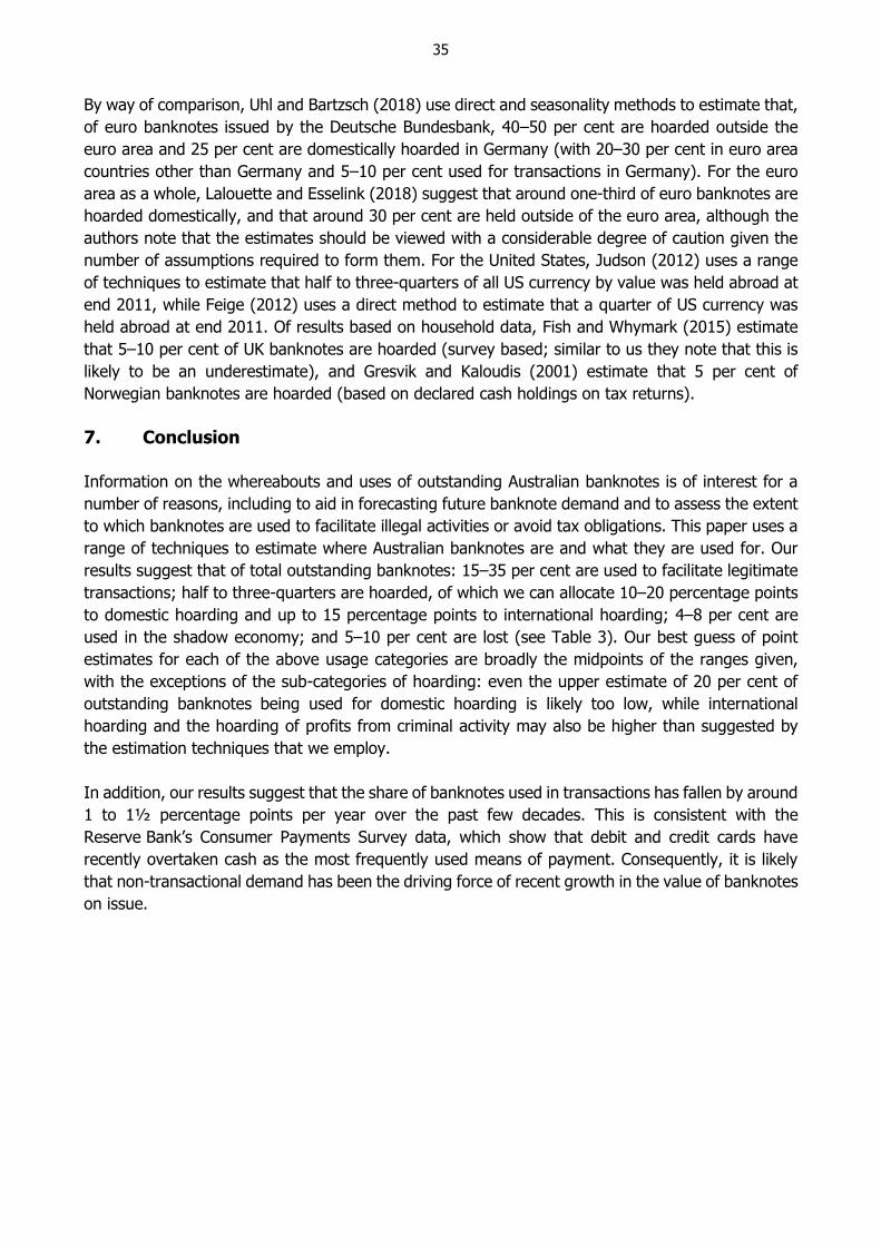
35

By way of comparison, Uhl and Bartzsch (2018) use direct and seasonality methods to estimate that,

of euro banknotes issued by the Deutsche Bundesbank, 40–50 per cent are hoarded outside the

euro area and 25 per cent are domestically hoarded in Germany (with 20–30 per cent in euro area

countries other than Germany and 5–10 per cent used for transactions in Germany). For the euro

area as a whole, Lalouette and Esselink (2018) suggest that around one-third of euro banknotes are

hoarded domestically, and that around 30 per cent are held outside of the euro area, although the

authors note that the estimates should be viewed with a considerable degree of caution given the

number of assumptions required to form them. For the United States, Judson (2012) uses a range

of techniques to estimate that half to three-quarters of all US currency by value was held abroad at

end 2011, while Feige (2012) uses a direct method to estimate that a quarter of US currency was

held abroad at end 2011. Of results based on household data, Fish and Whymark (2015) estimate

that 5–10 per cent of UK banknotes are hoarded (survey based; similar to us they note that this is

likely to be an underestimate), and Gresvik and Kaloudis (2001) estimate that 5 per cent of

Norwegian banknotes are hoarded (based on declared cash holdings on tax returns).

7. Conclusion

Information on the whereabouts and uses of outstanding Australian banknotes is of interest for a

number of reasons, including to aid in forecasting future banknote demand and to assess the extent

to which banknotes are used to facilitate illegal activities or avoid tax obligations. This paper uses a

range of techniques to estimate where Australian banknotes are and what they are used for. Our

results suggest that of total outstanding banknotes: 15–35 per cent are used to facilitate legitimate

transactions; half to three-quarters are hoarded, of which we can allocate 10–20 percentage points

to domestic hoarding and up to 15 percentage points to international hoarding; 4–8 per cent are

used in the shadow economy; and 5–10 per cent are lost (see Table 3). Our best guess of point

estimates for each of the above usage categories are broadly the midpoints of the ranges given,

with the exceptions of the sub-categories of hoarding: even the upper estimate of 20 per cent of

outstanding banknotes being used for domestic hoarding is likely too low, while international

hoarding and the hoarding of profits from criminal activity may also be higher than suggested by

the estimation techniques that we employ.

In addition, our results suggest that the share of banknotes used in transactions has fallen by around

1 to 1½ percentage points per year over the past few decades. This is consistent with the

Reserve Bank’s Consumer Payments Survey data, which show that debit and credit cards have

recently overtaken cash as the most frequently used means of payment. Consequently, it is likely

that non-transactional demand has been the driving force of recent growth in the value of banknotes

on issue.

36

Table 3: Summary of Banknote Share Estimates

Per cent of total banknotes outstanding

Estimated range Adjusted for shadow economy Central estimate

Transactional stock

Counting method 20

Banknote life(a) 20–35 15–30

Banknote processing(a) 40 35

Velocity method 20–30

Seasonality method(a) 20–30 15–25

Overall assessment(a) 20–40 15–35 25

Hoarded stock

Total – non transactional(b) 50–75 62.5

Domestic – fire-damaged claims 2–3

Domestic – CPS results 10–20

International – outflow less inflow 0–15

Shadow economy

Underground – ABS 3

Underground – BETF 5

Illicit spending – ABS 1

Illicit spending – BETF 2

Illicit spending – wastewater analysis 2

Illicit profits – wastewater analysis 0–1

Overall assessment 4–8 5

Lost banknotes 5–10 7.5

Notes: (a) Includes banknotes used transactionally in shadow economy activity

(b) Includes banknotes hoarded as illicit profits from shadow economy activity

37

Appendix A: Ground-up Calculations

A.1 Wallets

Participants in the Reserve Bank’s Consumer Payments Survey are asked how much cash they are

currently holding in their wallet. This information, coupled with population data from the ABS, can

be used to estimate the total stock of cash held in wallets.

To do this, participants in the CPS are split into cohorts based on age. Average wallet holdings for

each cohort are then calculated. Because the CPS only includes the adult population, those

aged 9–17 are assumed to hold half as much cash as those aged 18–24, and those aged less than

9 are assumed to hold no cash. To calculate the total stock of cash held in wallets at the time of the

CPS, average wallet holdings are multiplied by the number of people in Australia within each cohort.

A time series is generated by tracking the size of each cohort over time using population data from

the ABS, and adjusting wallet holdings for changes in the CPI.

The amount of cash held in participants’ wallets was asked in the 2010, 2013 and 2016 waves of

the CPS. The method outlined above produces different estimates depending on which wave of the

CPS is used. An average of the three series is used. Australian population data by age group are

only available to June 2017. To estimate cash held in wallets after June 2017, the June 2017 figure

was projected forward using average growth over the previous five years.

A.2 Financial Institution Holdings

Authorised deposit-taking institutions (ADIs) (broadly consisting of commercial banks, credit unions

and building societies) hold physical currency in ATMs, branches, and cash depots, with these

holdings reported to the Reserve Bank; we assume that the share by value of coins and foreign

currency is negligible. For non-ADIs, we estimate cash holdings as the number of ATMs deployed by

independent ATM deployers multiplied by an assumed average value held in each ATM set to 25 per

cent of their capacity.

A.3 Self-serve check-outs (SSCs)

The stock of cash held in SSCs is estimated using the number of cash-accepting SSCs in Australia

and the average amount of cash held per cash-accepting SSC.

The number of cash-accepting SSCs is estimated in three stages. First, the number of stores with

SSCs is approximated using the number of Coles, Woolworths, Kmart, Target, Big W and Bunnings

stores (found in the annual reports of Wesfarmers and Woolworths Group). Second, it is assumed

that the number of SSCs per store is zero in 2007, gradually rising to ten for Coles and Woolworths

and five for the other retailers by 2017. Finally, we assume that all SSCs accepted cash when they

were first introduced, but that the share of cash-accepting SSCs fell to 60 per cent over the following

decade. We assume that $10,000 is held by each SSC at the start of the day to be used as change

and for cash withdrawals (although our overall results are insensitive to this figure and are largely

unchanged if we instead use $3,000, for example).

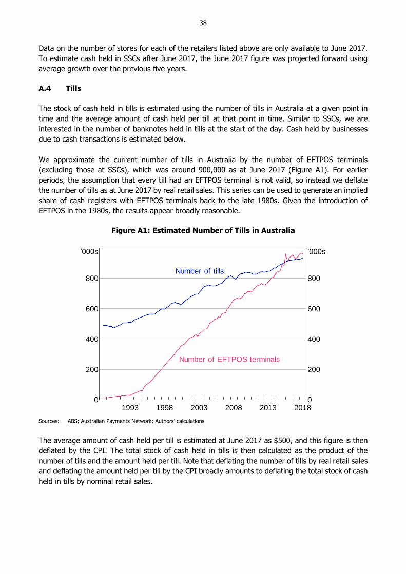
38

Data on the number of stores for each of the retailers listed above are only available to June 2017.

To estimate cash held in SSCs after June 2017, the June 2017 figure was projected forward using

average growth over the previous five years.

A.4 Tills

The stock of cash held in tills is estimated using the number of tills in Australia at a given point in

time and the average amount of cash held per till at that point in time. Similar to SSCs, we are

interested in the number of banknotes held in tills at the start of the day. Cash held by businesses

due to cash transactions is estimated below.

We approximate the current number of tills in Australia by the number of EFTPOS terminals

(excluding those at SSCs), which was around 900,000 as at June 2017 (Figure A1). For earlier

periods, the assumption that every till had an EFTPOS terminal is not valid, so instead we deflate

the number of tills as at June 2017 by real retail sales. This series can be used to generate an implied

share of cash registers with EFTPOS terminals back to the late 1980s. Given the introduction of

EFTPOS in the 1980s, the results appear broadly reasonable.

Figure A1: Estimated Number of Tills in Australia

Sources: ABS; Australian Payments Network; Authors’ calculations

The average amount of cash held per till is estimated at June 2017 as $500, and this figure is then

deflated by the CPI. The total stock of cash held in tills is then calculated as the product of the

number of tills and the amount held per till. Note that deflating the number of tills by real retail sales

and deflating the amount held per till by the CPI broadly amounts to deflating the total stock of cash

held in tills by nominal retail sales.

20132008200319981993 20180

200

400

600

800

’000s

0

200

400

600

800

’000s

Number of tills

Number of EFTPOS terminals

39

A.5 Businesses – Unbanked Cash Takings

In addition to cash floats held in SSCs and tills, businesses also hold cash that has been received via

consumer cash payments. Assuming that businesses bank such cash on a weekly basis, the total

stock of cash held by businesses due to cash transactions – unbanked cash takings – will be

approximately equal to half the value of weekly consumer cash transactions. We use the same

estimate of cash spending as in Section 4.4.1.

A.6 Gaming Machines

Queensland Treasury collects data on both the number and turnover of gaming machines in

Australia. While the number has been broadly stable since 2002 at around 200,000, turnover has

increased by around two-thirds, from $85 billion to $143 billion. Given this, we estimate the stock

of cash held in gaming machines based on the flows into gaming machines rather than the number

of gaming machines.

However, an important distinction needs to be made between turnover and the amount of cash put

in gaming machines. Turnover represents the amount bet, not the amount expended. And because

the state governments each specify a minimum win ratio – typically around 0.85 – gambling turnover

can far exceed the net amount of cash put in the gaming machine.24 To account for this, we use

Queensland Treasury’s measure of gambling expenditure (turnover less winnings) to approximate

the total flow of cash into gaming machines. To estimate the stock of cash held in gaming machines

at any point in time, we simply convert this flow to a weekly figure and divide by two. Similar to

businesses’ unbanked cash takings, we have assumed that gaming machines’ takings are banked

weekly.

Data on gambling expenditure are only available to June 2016. To estimate cash held in gaming

machines after June 2016, the June 2016 figure was projected forward using average growth over

the previous five years.

A.7 Tourists (and Other Overseas Visitors)

We estimate four components related to tourists’ holdings of Australian banknotes:

tourists in Australia holding banknotes obtained in Australia;

tourists in Australia holding banknotes obtained overseas;

tourists about to come to Australia holding banknotes obtained overseas; and

overseas foreign exchange businesses servicing tourists about to come to Australia.

24 For example, suppose you put $150 cash in the machine and bet in $1 increments until your money is entirely

expended. Given a win ratio of 0.85, you expect to lose 15 cents on each spin. But this would be split between the

loss of the $1 you bet, and the 85 cents you win. If you repeated this process until your money was expended, you

would on average have bet $1,000, winning $850 along the way but losing your initial $150. Here, turnover is $1,000,

winnings is $850, and net cash put in the machine is $150.

40

We start by splitting tourists’ total spending in Australia – from Tourism Research Australia (TRA) –

into various payment methods. First, tourists’ card payments can be approximated using data on

payments that were made with cards issued overseas. Second, tourists’ cash payments with

domestically sourced cash can be approximated by withdrawals from domestic ATMs using cards

issued overseas. Third, because tourists often earn income while in Australia, some share of tourists’

spending will include card payments made from Australian bank accounts and cash payments made

using ATM withdrawals from Australian bank accounts. We approximate this using data on income

earned in Australia by tourists from TRA.25 Without further data, the split between cash and card

purchases is held in the same ratio as payments made with cards issued overseas and domestic ATM

withdrawals using cards issued overseas. Finally, payments made using cash sourced overseas is

estimated as the residual. This is not a perfect calculation, with the estimated share of payments

made using cash sourced overseas occasionally turning negative. However, without more

information it is difficult to improve upon this calculation.

Spending with cash sourced domestically (i.e. through both cards issued overseas and via Australian

bank accounts) is converted to a stock in three steps:

1. average spending per tourist per night using domestically sourced cash is estimated by dividing

total spending using domestically sourced cash by the number of tourists in Australia and the

number of nights stayed in Australia per tourist;

2. this figure is converted to an average stock held per tourist by assuming that, on average,

tourists visit an ATM once every five days and hold a small buffer of cash equal to 10 per cent

of anticipated spending;

3. we then multiply this by the number of tourists in Australia per night to arrive at the total stock

of domestically sourced cash held by tourists in Australia.

The stock of cash sourced overseas held by tourists in Australia is similarly estimated. Total tourist

spending using cash sourced overseas is converted to an average spending per tourist value. Tourists

are then assumed to have initially entered Australia with a stock equal to this spending value, a

stock which is entirely extinguished before they leave Australia. The average stock held by each

tourist over the duration of their trip is then approximated by half of their initial stock. Multiplying

this amount by the number of tourists in Australia per night yields an estimate of the stock of

overseas sourced cash held by tourists in Australia. However, and as noted, estimated spending by

tourists using overseas sourced cash can be negative. In these periods we simply assume that

tourists’ stock of overseas sourced cash is zero.

The stock of cash held by tourists about to enter Australia can also be estimated using the spending

data. We simply assume that soon-to-be tourists acquire the stock of cash they intend to bring to

Australia one month prior to their trip. The total stock of cash held by tourists about to enter Australia

is then estimated as average intended spending in Australia with overseas sourced cash per tourist

multiplied by the number of tourists about to enter Australia.

25 Income from the sale of motor vehicles and the sale of other capital goods – which, based on the TRA data, comprise

only a small share of total income – is excluded on the assumption that most of this income will not be spent in

Australia.

41

Finally, we estimate the stock of cash held by overseas foreign exchange businesses by assuming

that they hold a stock of cash equal to two months’ worth of outflows (averaged over the previous

six months). Here, outflows refers to cash acquired by soon-to-be-tourists.

Data on tourism expenditure in Australia are only available to December 2017. To estimate all

components of cash held by tourists after December 2017, the December 2017 figures were

projected forward using their average values over the past year.

42

Appendix B: Banknote Life Calculations

By assumption all transactional banknotes have the same life span, denoted by k. We estimate k as

the average of total outstanding banknotes divided by destructions for the $5, $10 and $20

denominations. For the higher denominations, denoted H, the total outstanding includes both the

transactional and non-transactional banknotes. That is,

-H H HTot Trans Non trans

We assume that only transactional banknotes are destroyed, and that the average life of the

transaction stock of higher denomination banknotes matches that of the lower denominations, that

is:

H

H

Transk

Destr

Then

- -H H H H

H H H H

Tot Trans Non trans Non transk

Destr Destr Destr Destr

Rearranging, we have that

-

1

H

H HH

H H H

H

Totk

Non trans TransDestr

Tot Tot Tot

Destr

That is, the excess life of a high-denomination banknote divided by the life of that high-denomination

banknote is equal to the share of that denomination used for non-transactional purposes. Subtracting

this number from 1 gives us the transactional share.

43

Appendix C: Velocity Calculations

In this appendix, we justify multiplying the turnover rate by (1 + 2r). We deal with the case of

estimating the time cash spends in wallets, but note that the same logic applies to tills and ATMs.

Further, since we are only concerned about the flow of a generic dollar, not individual banknotes

per se, we assume that cash flows out of a wallet in the same order in which it flows in (first-in first-

out) and that cash is spent at a constant rate halfway through each day.

Case 1: No buffer stock. Suppose that the number of days between cash top-ups is n. Then 1/nth

of cash is spent at 0.5 days; the next 1/nth of cash is spent at 1.5 days; and so on, until the last 1/nth

of cash is spend at n – 0.5 days. The average time that any dollar spends in the wallet is:

1 1 3 1 1 1 1 1

1 2 12 2 2 2 2 2 2

n nn n

n n

We would estimate that cash spends n/2 days on average in a wallet.

Case 2: Buffer stock. Suppose again that the number of days between cash top-ups is n. If the

buffer share is r (where r is a number between 0 and 1), then we need to recognise that in any

period a person first spends their buffer stock from the previous period. The buffer stock is exhausted

after (rn – 0.5) days. Any cash spent from the buffer spends (n + b + 0.5) days in the wallet, where

b is the number of days since the most recent top-up and is an integer in [0, rn – 1]. Cash that is

not part of the previous buffer is then spent from the rn + 0.5 day until the n – 0.5 day. The average

time that a dollar spends in the wallet is then:

20.5 1.5 0.5 0.5 0.5 0.5 1.5 0.5

1 22 2

n n n rn rn n rn n

n n

n nrn r

This is the formula we use.

44

References

ABS (Australian Bureau of Statistics) (2013), ‘Information Paper: The Non-Observed Economy and

Australia's GDP, 2012’, ABS Cat No 5204.0.55.008, viewed 4 July 2018.

ACIC (Australian Criminal Intelligence Commission) (2017), 2016–17 Annual Report.

ACIC (2018a), Illicit Drug Data Report 2016–17.

ACIC (2018b), National Wastewater Drug Monitoring Program, Report 4, March.

AIHW (Australian Institute of Health and Welfare) (2017), National Drug Strategy Household Survey

2016: Detailed Findings, Drug Statistics Series No 31, Cat No PHE 214, AIHW, Canberra.

Bank of Finland (Suomen Pankki) (2012), ‘Returning Markka to the Bank of Finland’, viewed 4 July 2018.

Available at <https://www.suomenpankki.fi/en/money-and-payments/the-markka2/returning-markka-to-the-

bank-of-finland/>.

Bartzsch N, Rösl G and F Seitz (2011), ‘Foreign Demand for Euro Banknotes Issued in Germany:

Estimation Using Indirect Approaches’, Deutsche Bundesbank Discussion Paper Series 1: Economic Studies

No 21/2011.

BETF (Black Economy Taskforce) (2017), Black Economy Taskforce: Final Report – October 2017,

(M Andrew, Chair), Australian Treasury, Canberra.

Boeschoten WC (1992), Currency Use and Payments Patterns, Financial and Monetary Policy Studies, 23,

Kluwer Academic Publishers, Dordrecht.

Davies C, M-A Doyle, C Fisher and S Nightingale (2016), ‘The Future of Cash’, RBA Bulletin, December,

pp 43–52.

Doyle M-A, C Fisher, E Tellez and A Yadav (2017), ‘How Australians Pay: Evidence from the 2016

Consumer Payments Survey’, RBA Research Discussion Paper No 2017-04.

Feige EL (2012), ‘The Myth of the “Cashless Society”: How Much of America’s Currency is Overseas?’, The

Usage, Costs and Benefits of Cash: Theory and Evidence from Macro and Micro Data, Papers from the

International Cash Conference, Deutsche Bundesbank, Frankfurt am Main, pp 119–151.

Fish T and R Whymark (2015), ‘How Has Cash Usage Evolved in Recent Decades? What Might Drive

Demand in the Future?’, Bank of England Quarterly Bulletin, 55(3) Q3, pp 216–227.

Flannigan G and S Parsons (2018), ‘High-Denomination Banknotes in Circulation: A Cross-Country

Analysis’, RBA Bulletin, March, viewed 4 July 2018. Available at <https://www.rba.gov.au/

publications/bulletin/2018/mar/high-denomination-banknotes-in-circulation-a-cross-country-analysis.html>.

Flannigan G and A Staib (2017), ‘The Growing Demand for Cash’, RBA Bulletin, September, pp 63–74.

Gresvik O and A Kaloudis (2001), ‘Increased Cash Holdings – Reduced Use of Cash: A Paradox?’, Norges

Bank Economic Bulletin, No 4/2001, pp 134–139.

https://www.rba.gov.au/publications/bulletin/2017/sep/pdf/bu-0917-8-the-growing-demand-for-cash.pdf

https://www.rba.gov.au/publications/bulletin/2017/sep/pdf/bu-0917-8-the-growing-demand-for-cash.pdf

45

Guibourg G and B Segendorf (2007), ‘The Use of Cash and the Size of the Shadow Economy in Sweden’,

Sveriges Riksbank Working Paper Series No 204.

Gyomai G and P van de Ven (2014), ‘The Non-Observed Economy in the System of National Accounts’,

OECD Statistics Brief No 18. Available at <https://www.oecd.org/sdd/na/Statistics%20Brief%2018.pdf>.

Humphrey D, A Kaloudis and G Øwre (2004), ‘The Future of Cash: Falling Legal Use and Implications for

Government Policy’, Journal of International Financial Markets, Institutions and Money, 14(3), pp 221–233.

Judson R (2012), ‘Crisis and Calm: Demand for U.S. Currency at Home and Abroad from the Fall of the

Berlin Wall to 2011’, Board of Governors of the Federal Reserve System International Finance Discussion

Paper IFDP 1058.

Karlsson A and L Burns (2017), Australian Drug Trends 2017: Findings from the Illicit Drug Reporting

System (IDRS), Australian Drug Trends Series No 181, National Drug and Alcohol Research Centre, Sydney.

Available at <https://ndarc.med.unsw.edu.au/resource/illicit-drug-reporting-system-idrs-national-report-

2017>.

Lalouette L and H Esselink (2018), ‘Trends and Developments in the Use of Euro Cash over the past Ten

Years’, ECB Economic Bulletin, No 6/2018, pp 87–109.

Lowe P (2018), ‘Remarks at Reserve Bank Board Dinner’, Adelaide, 1 May

Medina L and F Schneider (2018), ‘Shadow Economies around the World: What Did We Learn over the

Last 20 Years?’, IMF Working Paper No WP/18/17.

OECD, IMF, ILO and CIS Stat (Organisation for Economic Co-operation and Development,

International Monetary Fund, International Labour Organization and Interstate Statistical

Committee of the Commonwealth of Independent States) (2002), Measuring the Non-Observed

Economy: A Handbook, OECD Publishing, Paris.

Pickhardt M and J Sardà (2012), ‘Cash, Hoarding and the Underground Economy’, The Usage, Costs and

Benefits of Cash: Theory and Evidence from Macro and Micro Data, Papers from the International Cash

Conference, Deutsche Bundesbank, Frankfurt am Main, pp 15–45.

Rush A (2015), ‘The Life of Australian Banknotes’, RBA Research Discussion Paper No 2015-10.

Schneider F, A Buehn and CE Montenegro (2010), ‘Shadow Economies All over the World: New Estimates

for 162 Countries from 1999 to 2007 (Revised Version)’, World Bank Policy Research Working Paper 5356.

Seitz F (2007), ‘A Simple Way to Capture Transaction Balances’, Economics Letters, 95(2), pp 230–233.

Snellman JS, JM Vesala and DB Humphrey (2001), ‘Substitution of Noncash Payment Instruments for

Cash in Europe’, Journal of Financial Services Research, 19(2–3), pp 131–145.

Stenkula M (2004), ‘The Euro Cash Changeover Process’, Kyklos, 57(2), pp 265–286.

Sumner SB (1990), ‘The Transactions and Hoarding Demand for Currency’, Quarterly Review of Economics

and Business, 30(1), pp 75–89.

46

Sveriges Riksbank (2018), ‘Statistics on Notes and Coins’, viewed 4 July 2018. Available at

<https://www.riksbank.se/en-gb/notes-and-coins/statistics/>.

Uhl M and N Bartzsch (2018), ‘Domestic and Foreign Demand for Euro Banknotes Issued in Germany’, War

on Cash: Is there a Future for Cash?, Papers from the International Cash Conference, Deutsche Bundesbank,

Frankfurt am Main, pp 251–286.

where’s the money‽ an investigation into the whereabouts ... · where’s the money‽ an...

Documents