Where did the laws of physics come from?Victor J. Stenger

Department of Philosophy, University of Colorado at Boulder

Boulder, Colorado

Department of Physics and Astronomy, University of Hawaii at Manoa

Honolulu, Hawaii

E-mail: vstenger@mindspring.com

Abstract

The laws of physics are constrained so that they select out no preferred coordinate

system or reference frame. This is called the principle of covariance. This principle can be

further generalized to include the coordinates in the abstract space of the functions used

to formulate those laws. This is called global gauge invariance. When this symmetry

applies independently at every point in space-time, it is called local gauge invariance.

These symmetries are almost all that are needed to derive most of the familiar laws the

law of physics, including classical mechanics, the great conservation laws, quantum

mechanics, special and general relativity, and electromagnetism. Those structures that

do not follow directly from coordinate invariance result from spontaneously broken

symmetries.

PACS numbers: 01.55, 01.70, 11.30, 11.30E, 14.80.C

1.0 Introduction

Most laypeople think of the laws of physics as something like the Ten

Commandments—rules governing the behavior of matter imposed by some great

lawgiver in the sky. However, no stone tablet has ever been found upon which such

laws were either naturally or supernaturally inscribed. On the contrary, the laws of

1

physics are human inventions—mathematical formulas that quantitatively describe the

results of observations and measurements. These formulas are first inferred from and

then tested against observations. If they hold up, they are eventually reformulated as

part of general and universal theories that are derived from a minimum number of

assumed fundamental principles. Very often, a "law" will turn out to be nothing more

than a circular definition, such as Ohm's law which says that the voltage is proportional

to the current in a resistor, where a resistor is defined as a device that obeys Ohm's law.

Since the time of Copernicus and Galileo it has been realized that the laws of

physics should not single out any particular space-time reference frame, although a

distinction between inertial and noninertial frames was maintained in Newtonian

physics. That distinction was removed in 1916 by Einstein who formulated his general

theory of relativity in a covariant way. That is, the form of Einstein's equations is the

same in all reference frames, inertial or noninertial.

As this experience showed, physicists are highly constrained in the way they

may formulate the laws of physics. Not only must they agree with the data, the

equations that are used to describe that data should not be written in such a way as to

specify a privileged coordinate system or reference frame. This principle of covariance

generalizes other notions such as the Copernican and cosmological principles and the

principle of Galilean relativity. The application of this principle is not a matter of choice;

centuries of observations have shown that to do otherwise produces calculations that

disagree with the data in some reference frames.

In 1918, Noether showed that coordinate independence was more than just a

constraint on the mathematical form of physical laws.[1] She proved that some of the

most important physics principles are, in fact, nothing more than tautologies that follow

from space-time coordinate independence: energy conservation arises from time

translation invariance, linear momentum conservation comes from space translation

invariance, and angular momentum conservation is a consequence of space rotation

invariance. These conserved quantities were simply the mathematical generators of the

2

corresponding symmetry transformation.

As the twentieth century progressed, invariance or symmetry principles became

an increasingly dominant idea in physics. Not only were space-time coordinate

symmetries built into theories, the notion of coordinate independence was extended to

the abstract spaces physicists use to represent the other degrees of freedom of systems.

Rotational symmetry was also applied to the space of quantum state vectors, resulting

in derived properties of spin, isospin, charge, baryon number, and other observables

that agreed with measurements.

Charge conservation, for example, was found to follow from the invariance of

the Schrödinger equation to changes in the phase of the complex wave function. And

then, a remarkable discovery was made. It was found that the Schrödinger equation

could be made invariant to a local phase change in the wave function, that is, a change in

phase that varies from point to point in space-time, provided that vector and scalar

potentials were added. The potentials turned out to be exactly those that give the

classical electric and magnetic fields. This local quantum phase symmetry was precisely

related to the local classical gauge symmetry of electrodynamics. Maxwell's equations

were derived from a single principle—local phase invariance.

If we think of the Schrödinger wave function as a "vector" in 2-dimensional

complex space, then changing phase is equivalent to a rotation in that space and phase

invariance, or gauge invariance, is equivalent to rotational invariance. Indeed, the

generator of that transformation is the electric charge whose conservation follows from

global gauge invariance.

In the standard model, the fields associated with the weak and strong nuclear

forces are obtained by extending the idea of gauge symmetry to higher dimensions of

abstract space. There the situation is complicated by the fact that all the symmetries are

not exact at the "low temperatures" of current experimentation. Good thing. The

diversity and complexity of the universe is a result of broken symmetries, without

which we would not be here to do the experiments.

3

Twentieth century physics was also marked by the discovery that symmetries

are often broken. In the 1950s, it was found that weak interactions maximally violated

space reflection symmetry; that is, they were not invariant under the parity operation P

that changes the handedness or chirality of a system. In the 1960s certain rare decays

were found to be noninvariant under the combined operation CP, where C changes a

particle to its antiparticle. The study of the origin of CP violation remains a subject of

considerable experimental and theoretical effort to this date.

In this paper, it will be shown that much of familiar physics can be derived from

the generalized notion of coordinate invariance applied not only in space-time but in

the spaces of other observables and the spaces of the functions that are used to

mathematically describe physical phenomena. In order to make this result accessible to

the greatest number of people, the mathematical level will be limited to that of an

advanced undergraduate student in physics or mathematics. The equations will appear

very familiar—just those found in physics textbooks, and it may appear that the author

is using hindsight to make things come out the way they already are. However, the

reader is asked to look carefully at how those equations are obtained. Certain familiar

principles normally taken as axioms, such as the quantization of angular momentum

and the invariance of the speed of light will be derived from the hypothesized

symmetry principles without additional assumptions.

2.0 Gauge Symmetry

Let q = (qo, q1, q2, q3, . . . qn ) be the set of observables of a physical system such as a

particle or group of particles and take them to be the coordinates of an n-dimensional

vector q in q-space. Spatial coordinates and time are included and placed on the same

footing as the other observables. Thus a point in q-space, designated by the vector q,

represents a particular set of measurements on a system. The generalized principle of

covariance says that the laws of physics must be the same for any origin or orientation

4

of q, that us, any choice of coordinate system.

Let us define a vector y in another multidimensional space we will call y-space.

Assume y = y(q). The state vectors of quantum mechanics are familiar examples of y-

space vectors. We can imagine a set of coordinate axes in y-space. Extending the notion

of covariance to this space we will assume that the following principle holds: the laws of

physics cannot depend on the orientation of the vector y in y-space. This principle is called

gauge symmetry.

3. Gauge Transformations and their Generators

To get started as simply as possible, let us take y(q) to be a complex function, that is, a

2-dimensional vector with coordinates (Re{y }, Im{y }). Let us perform a unitary

transformation on y:

y' = Uy (3.1)

where U†U = 1, so

y†y' = y†U†Uy= y†y (3.2)

This transformation does not change the magnitude of y,

|y'| = (y'†y' )1/2 = (y†y )1/2 = |y| (3.3)

That is, |y| is invariant to the transformation, as required by gauge symmetry. We can

write the operator U

5

U = exp(iq) (3.4)

where q† = q, that is, q is a hermitian operator. Then,

y' = exp(iq) y (3.5)

So, U simply changes the complex phase of y. It could be called a "phase

transformation," or just simply a unitary transformation. However, in the

amplifications of this idea that we will discussing, the designation "gauge

transformation" has become conventional. When q is a constant we have a global gauge

transformation.When q is a not a constant but a function of position and time it is called

a local gauge transformation.

Note also that the operation U corresponds to a rotation in the complex space of

y. Later we will generalize these ideas to where y is a vector in higher dimensions and q

will be represented by a matrix. But this basic idea of a gauge transformation as

analogous to a rotation in an abstract function space will be maintained and gauge

invariance viewed as an invariance under such rotations.

Let us write

q = eG (3.6)

where e is an infinitesimal number and G is another operator. Then

U ≈ 1 + ieG (3.7)

.

where G† = G is hermitian and is called the generator of the transformation. Then,

6

y' ≈ y + ie G y (3.8)

Suppose we have a transformation that takes the variable qm to q'm = qm + em.

Then

y'(q'm ) = y(qm + em ) ≈ y(qm ) + em ∂y/∂qm (3.9)

It follows that the generator can be written

Gm = -i∂/∂qm (3.10)

Define

†

Pm ≡ hG = -ih ∂

∂qm

(3.11)

where

†

h is an arbitrary constant introduced only if you want the units of Pm to be

different from the reciprocal of the units of qm. The transformation operator can then be

written

†

U = 1 +∂

∂qm (3.12)

For example, suppose that q1 = x, the x-coordinate of a particle. Then

7

†

P1 ≡ Px = -ih ∂

∂x (3.13)

which we recognize as the quantum mechanical operator for the x-component of

momentum. Note that this association was not assumed but derived and no connection

with mass and velocity has yet been made. This just happens to be the form of the

generator of a space translation. Similarly, we can take q2 = y, q3 = z and obtain the

generators Py and Pz .

It may also be noted that q might contain operationally defined momenta, in

which case spatial coordinates would then be introduced in the manner of (3.13).

Of course,

†

h will turn out to be the familiar quantum of action of quantum

mechanics,

†

h = h/2π where h is Planck's constant. Physicists often take

†

h = 1 in "natural

units." We will leave

†

h in our equations at this point to maintain familiarity, however it

should be recognized that this constant, when expressed in non-dimensionless units,

will turn out to be an arbitrary number determined only by that choice of units. No

additional physical assumption about the "quantization of action" need be made and

Planck's constant should not be viewed as a metric constant of nature. In particular,

†

h

cannot be zero. Once we have made the connection of (Px, Py, Pz) with the 3-

momentum, quantization of action will already be in place.

We can also associate one of the variables, say qo with the time t. In order to

provide a connection with the fully relativistic treatment we will make later, let qo ≡ ict,

where c is, like

†

h , another arbitrary conversion factor. Later we will associate it with the

speed of light in a vacuum and find (not assume) that it is a Lorentz invariant. For now,

†

Po = ih ∂

∂qo= -

h

c∂

∂t (3.14)

8

We can then define

†

H ≡ -iPoc = ih ∂

∂t (3.15)

which we recognize as the quantum mechanical Hamiltonian (energy) operator. Note,

again, that this familiar result was not assumed but derived. No connection with the

physical quantity energy has yet been made. This just happens to be the form of the

generator of a time translation.

4. Quantum Mechanics from Gauge Transformations

Suppose we have a complex function y(x, y, z, t) that describes, in some unspecified

way, the state of a system. It will evolve with time according to

†

Hy = ih ∂

∂t(4.1)

This is the time-dependent Schrödinger equation of quantum mechanics, where y is

interpreted as the wave function. If H is independent of time, we have the solution

†

y(t) =y(0)exp -ih

HtÊ

Ë Á

ˆ

¯ ˜ (4.2)

so

†

U(t) = exp -ih

HtÊ

Ë Á

ˆ

¯ ˜ (4.3)

9

is the time evolution operator.

At this point, then, we have the makings of quantum mechanics with no physical

assumptions whatsoever. That is, we have a mathematical theory that looks like

quantum mechanics although we have not yet identified the operators H and P with the

physics quantities energy and momentum. We have simply noted that these are

generators of time and space translations respectively, which are themselves gauge

transformations.

Let us proceed along these same lines, considering only the mathematics of

gauge transformations and leaving the physics to later. This does not stop us from

using the Dirac bra and ket notation for linear vectors and operators. Again, no physical

assumption is being made. We are simply using a convenient mathematical formalism.

So, let

†

y be a linear vector and

†

y be its dual. For simplicity, we take our linear

vectors to have unit norm,

†

y y = 1 (4.4)

A unitary transformation on

†

y will preserve the norm.

†

¢ y =U y > (4.5)

†

y U†U y = 1 (4.6)

Let A be a linear operator that gives another vector of unit norm

†

f = Ay (4.7)

10

Then,

†

f Ay = 1 (4.8)

and

†

f U† AU y = ¢ f Ay = ¢ f ¢ f = 1 (4.9)

We can define

A' = U†A U (4.10)

and write

†

f ¢ A y = 1 (4.11)

Let us consider the specific case where U is the time evolution operator,

†

y(t) =U y(0) (4.12)

In that case,

†

f(0) U† AU y(0) = f(t ) Ay(t) = f(t ) f(t) = 1 (4.13)

Alternatively, define

11

†

A(t) = U† A(0)U (4.14)

Then,

†

f(0) A(t) y(0) = 1 (4.15)

This illustrates the two approaches to time evolution in quantum mechanics. In

the Schrödinger picture, the state vector varies with time while the operators stay fixed.

In the Heisenberg picture, the state vectors remain fixed while the operators evolve

with time.

If we now interpret, in usual quantum mechanical fashion, the state vectors in

terms of probabilities and the operators in terms of observables, the expectation value

for the observable A, the mean value expected for an ensemble of measurements of A

when the system is in the state

†

y(0) is, in the Schrödinger picture,

†

A(0) = y(0) Ay(0) (4.16)

It evolves with time according to

†

A(t) = y(t) Ay(t) (4.17)

where

†

y(t) =U y(0) (4.18)

12

In the Heisenberg picture we have

†

A(0) = y(0) A(0)y(0) (4.19)

and

†

A(t) = y(0) A(t)y(0) (4.20)

where

†

A(t) = U† A(0)U = exp ih

HtÊ

Ë Á

ˆ

¯ ˜ A(0)exp -

ih

HtÊ

Ë Á

ˆ

¯ ˜ (4.21)

Let us look further at the time evolution of operators. Suppose we make an

infinitesimal transformation in time t Æ t + dt. Then

†

U(t) = 1 -ih

Ht (4.22)

†

A(t + dt) = 1+ih

HtÊ

Ë Á

ˆ

¯ ˜ A(t) 1-

ih

HtÊ

Ë Á

ˆ

¯ ˜ = A(t) -

ih

A, H[ ] (4.23)

Since

†

A(t + dt) = a(t) + dt ∂A∂t

(4.24)

13

it follows that

†

∂A∂t

= -ih

A,H[ ] (4.25)

The time rate of change of an observable then is

†

dAdt

=∂A∂t

+∂A∂qkk≠0

 dq kdt

(4.26)

or,

†

dAdt

= -ih

A, H[ ] +∂A∂qkk=1

n dqk

dt(4.27)

where the sum excludes the time variable.

Now we move to gauge transformations involving the non-temporal variables

of a system. Consider the case where A = Pj. Then,

†

dPj

dt= -

ih

Pj ,H[ ] +∂Pj

∂qkk=1

n dq k

dt(4.28)

Next, let us look at the transformation of these non-temporal variables. Let the variable

†

qk Æ qk +ek , where ek is infinitesimal. Then, as we saw above, the transformation

14

operator is

†

U = 1 +ih

Pkek (4.29)

Thus,

†

y(qk +ek) = y(qk) +ih

Pkek y(qk ) (4.30)

Suppose we have an operator A defined by

†

Ay(qk ) = f(qk) (4.31)

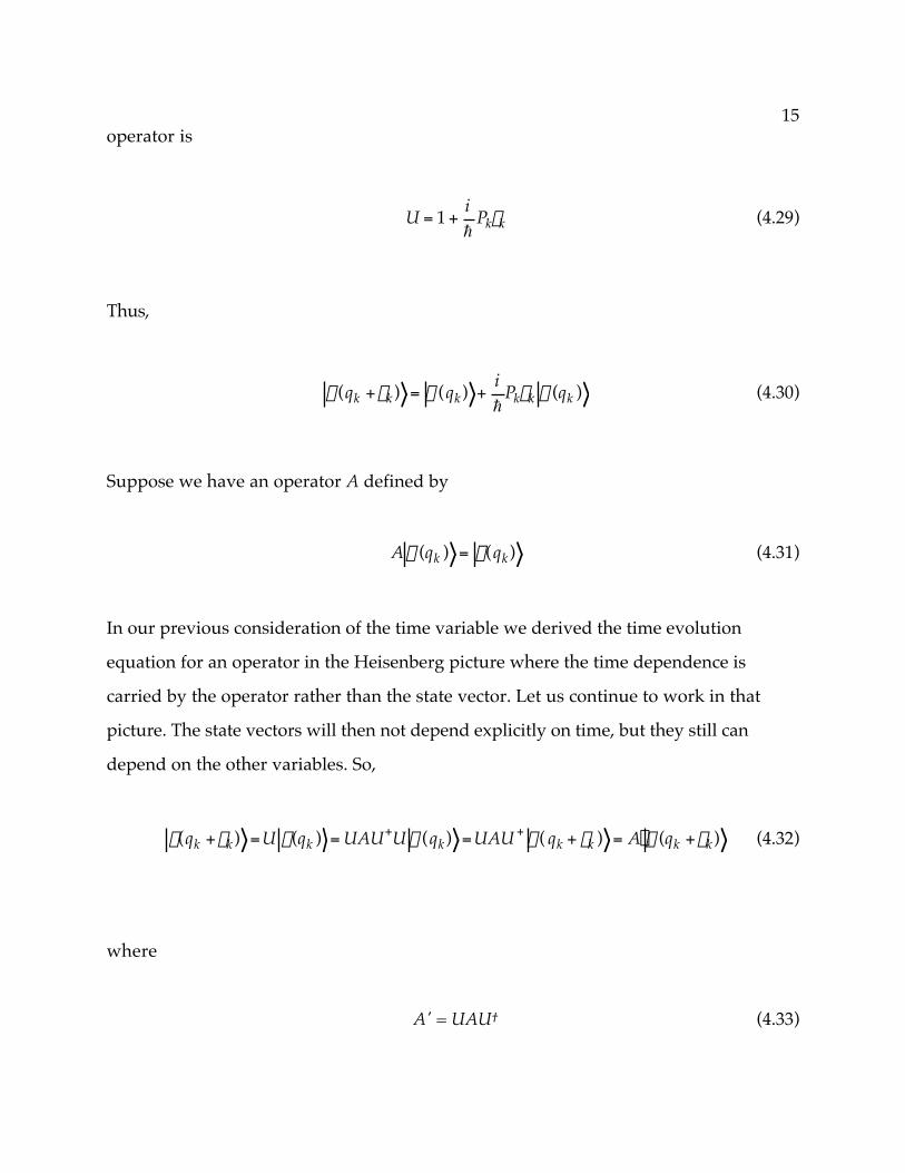
In our previous consideration of the time variable we derived the time evolution

equation for an operator in the Heisenberg picture where the time dependence is

carried by the operator rather than the state vector. Let us continue to work in that

picture. The state vectors will then not depend explicitly on time, but they still can

depend on the other variables. So,

†

f(qk +ek) =U f(qk ) = UAU+U y(qk) =UAU + y( qk + ek ) = ¢ A y(qk +ek) (4.32)

where

A' = UAU† (4.33)

15

We can write this

†

¢ A = 1+ih

PkekÊ

Ë Á

ˆ

¯ ˜ A 1-

ih

PkekÊ

Ë Á

ˆ

¯ ˜ = 1-

ih

A, Pk[ ] (4.34)

so,

†

∂A∂qk

= -ih

A,Pk[ ] (4.35)

From the differential form of the operators Pk,

†

Pj , Pk[ ] = 0 (4.36)

for j ≠ k, and so

†

∂Pj

∂qk= 0 (4.37)

Recall (4.28),

†

dPkdt

= -ih

Pk ,H[ ] +∂Pk∂q jj

Âdqj

dt(4.38)

The summed terms are all zero, so

16

†

dPkdt

= -ih

Pk ,H[ ] (4.39)

We can also think of qk as an operator, so

†

∂qk∂qk

= 1 = -ih

qk ,Pk[ ] (4.40)

or,

†

q k ,Pk[ ] = ih (4.41)

This can also be seen from

†

q k ,Pk[ ]y = qk , hi

∂

∂q k

È

Î Í

˘

˚ ˙ y =

h

iqk

∂y∂qk

-h

i∂

∂qkqky = ihy (4.42)

For example,

†

x ,Px[ ] = ih (4.43)

the familiar quantum mechanical commutation relation.

Now, we can also write

17

†

∂H∂qk

=h

iH, Pk[ ] (4.44)

Thus,

†

dPkdt

= -∂H∂qk

(4.45)

which is the operator version of one of Hamilton's classical equations of motion and

another way of writing Newton's second law of motion. Here we see that we have

developed another profound concept, from gauge invariance alone. When the

Hamiltonian of a system does not depend on a particular variable, then the observable

corresponding to the generator of the gauge transformation of that variable is

conserved. This is a version of Noether's theorem mentioned in the Introduction.

From this point, the rest of quantum mechanics can be developed. Observables

A are represented as hermitian operators and the expectation value of A is

†

A = y Ay (4.46)

The possible results of a measurement of A is determined by the solutions of the

eigenvalue equation

†

A a = a a (4.47)

where

†

a is the eigenstate of A corresponding to eigenvalue a. When the state of a

system is an eigenstate of an observable, the measurement of that observable will

18

always yield the eigenvalue corresponding to that state.

The symbol

†

a a stands for an operator that projects

†

y onto the

†

a axis.

When the eigenvectors

†

a form a complete set,

†

aa

 a = 1 (4.48)

In that case, the state vector of a system will be the linear combination

†

y = aa

 a y (4.49)

where

†

a y2 is the probability for

†

y to be found in the eigenstate

†

a . The wave

function is defined as the inner product

†

y(q) = q y (4.50)

where

†

q are the eigenstates of the spatial coordinates (or space-time coordinates

relativistically) of the particles of the system. Momentum-space wave functions are also

often used.

More generally, the eigenstates

†

q are the basis states of a particular, arbitrary

representation, like the unit vectors i, j, and k of the Cartesian coordinate axes x, y, z.

y(q) is the projection of

†

y on

†

q .

We can represent y and q as column matrices. Then

19

†

y(q) = y i†

i qi (4.51)

where

†

yi† is a row matrix.

In this representation, the observable A is a square matrix,

†

A = yi†

i, j Aijy j (4.52)

or simply given by the matrix equation,

†

A =y† Ay (4.53)

Thus, the gauge transformation can be written

†

¢ y = Uy = exp(iq )y (4.54)

where U and q, and the corresponding generators, are square matrices.

5.0 Rotation and Angular Momentum

The variables (q1, q2, q3) can be identified with the coordinates (x, y, z) of a particle and

the corresponding momentum components are the generators of translations of these

coordinates. (In this formulation, nothing prevents other particles being included with

their space-time variables associated with other sets of four q's; note that by having

each particle carry its own time coordinate we can maintain a fully relativistic scheme.)

These coordinates can equally well be angular variables and the conjugate

20

momenta the corresponding angular momenta. These angular momenta will be

conserved when the Hamiltonian is invariant to the gauge transformations that

correspond to displacements of the corresponding angles. In this case, the

displacements will be rotations about the spatial axes. For example, if we take (q1,$q2,$q3)

= (fx,$fy,$fz ), where fx is the angle of rotation about the x-axis, etc., then the generators

of the rotations about these axes will be the angular momentum components

(Lx,Ly,$Lz). Rotational invariance about any of these axes will lead to conservation of

angular momentum about that axis.

Let us look for a moment at rotations in familiar 3-dimensional space. Suppose

we have a vector V = (Vx, Vy) in the x-y plane. Let is rotate it counter clockwise about

the z-axis by an angle f. We can write the transformation as a matrix equation:

†

¢ V x¢ V y

Ê

Ë Á Á

ˆ

¯ ˜ ˜ =

cosf -sinf

sinf cosf

Ê

Ë Á

ˆ

¯ ˜

VxVy

Ê

Ë Á Á

ˆ

¯ ˜ ˜ (5.1)

Specifically, let us consider an infinitesimal rotation of the position vector r = (x, y) by df

about the z-axis. From above,

†

¢ x ¢ y

Ê

Ë Á

ˆ

¯ ˜ =

1 -df

df 1Ê

Ë Á

ˆ

¯ ˜

xy

Ê

Ë Á

ˆ

¯ ˜ =

x - ydf

y + xdf

Ê

Ë Á

ˆ

¯ ˜ (5.2)

And so,

dx = -ydf (5.3)

and

21

dy = x df (5.4)

For any function f(x, y),

†

f (x + dx, y + dy) = f (x ,y) + dx ∂f∂x

+ dy ∂f∂y

(5.5)

to first order. Or, we can write (reusing the function symbol f ),

†

f (f + df) = f (f) - ydf∂f∂x

+ xdf∂f∂y

(5.6)

†

= f (f) + idfGf

where

†

G = -i x ∂

∂y- y ∂

∂xÊ

Ë Á

ˆ

¯ ˜ = xPy - yPx = Lz (5.7)

the angular momentum about z. Similarly,

Lx = yPz - zPy (5.8)

and

Ly = zPx - xPz (5.9)

This result can be generalized as follows. If you have function that depends on a spatial

22

position vector r = (x, y, z), and you rotate that position vector by an angle q about an

arbitrary axis, then that function transforms as

f'(r) = exp(iL•q )f(r) (5.10)

where the direction of q is the direction of the axis of rotation. Once again this has the

form of a gauge transformation, or phase transformation in f, where

U = exp (i L•q ) (5.11)

From the previous commutation rules one can show that the generators Lx, Ly,

and Lz do not mutually commute. Rather,

†

Lx ,Ly[ ] = ihLz (5.12)

and cyclic permutations. Thus the order of successive rotations is important.

Most quantum mechanics textbooks will contain the proof of the following

result, although it is not always stated so generally: Any vector operator J whose

components obey the angular momentum commutation rules,

†

Jx , Jy[ ] = ihJ z (5.13)

will have the following eigenvalue equations:

†

J2 j ,m = j(j + 1)h2 j ,m (5.14)

23

where

†

J2 = Jx2 + Jy

2 + Jz2 is the square of the magnitude of J.

†

Jz j ,m = mh j ,m (5.15)

where m goes from -j to + j in steps of one: m = -j, -j+1, . . . ,j-1, j. This implies that j is an

integer (including zero) or a half-integer.

6. Rotation and Gauge Transformations

We have already noted that the gauge transformation is like a rotation in the complex

space of a function. Let us now generalize that concept.

Again, it is important not to confuse the two different spaces involved in our

discussion. First we have the space spanned by the variables {q} of a system. We have

generally taken the first four of these to be the subspace of 4-dimensional space-time in

which we describe events. If our "system" contains more than one event, then

additional groups of 4-dimensional subspaces can be reserved for these. Other

subspaces are left available for other variables.

Besides q-space, an additional abstract space have alread introudced as y-space is

used to describe the quantum state of a system. That space has coordinate axes that are

defined by an arbitrary choice of basis vectors of the system

†

q , where if Q is the

operator corresponding to an observable,

†

Q q = q q (6.1)

Thus,

24

†

y = cii

 qi (6.2)

The basis states are usually taken to be orthonormal, that is,

†

qi qj = dij (6.3)

so

†

y y = 1 and

†

ci2

= qi y2 is the probability for a measurement of Q giving the

value qi when the system is in the state

†

y .

For example, the basis states are frequently chosen to be

†

x ,

†

y , and

†

z , where

the observables are all the possible coordinates of a particle, that is, all the eigenstates of

the eigenvalue equation

†

X x = x x (6.5)

The quantity

†

y(x) = x y is, for historical reasons, called the wave function, although it

often has nothng to do with waves. Since x is usually regarded as a continuous variable,

y-space is infinite dimensional. That is,

†

x is not one axis but an infinite number of

axes, one for every real number x. Even if we assume that x is discrete in units of the

Planck length, and space is finite, we still have an awfully large number of dimensions.

If the particle is an electron, then y-space may also include the basis states

†

+ 12

and

†

- 12 that are the eigenstates of the z-component of spin of the electron. Even

though spatial coordinates are more familiar than spins, 2-dimensional spin subspace is

a lot easier to visualize than the subspace of spatial coordinate eigenstates.

25

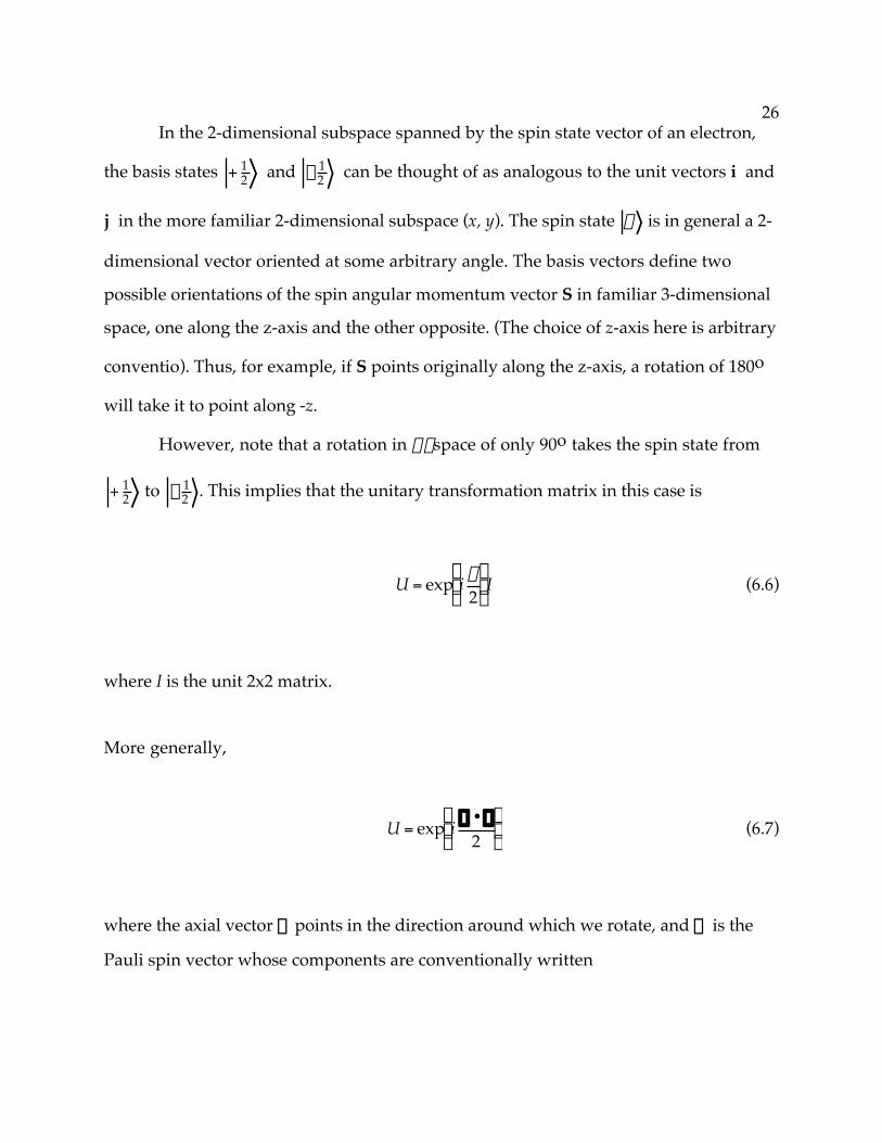
In the 2-dimensional subspace spanned by the spin state vector of an electron,

the basis states

†

+ 12 and

†

- 12 can be thought of as analogous to the unit vectors i and

j in the more familiar 2-dimensional subspace (x, y). The spin state

†

y is in general a 2-

dimensional vector oriented at some arbitrary angle. The basis vectors define two

possible orientations of the spin angular momentum vector S in familiar 3-dimensional

space, one along the z-axis and the other opposite. (The choice of z-axis here is arbitrary

conventio). Thus, for example, if S points originally along the z-axis, a rotation of 180o

will take it to point along -z.

However, note that a rotation in y-space of only 90o takes the spin state from

†

+ 12 to

†

- 12 . This implies that the unitary transformation matrix in this case is

†

U = exp i q2

Ê

Ë Á

ˆ

¯ ˜ I (6.6)

where I is the unit 2x2 matrix.

More generally,

†

U = exp i s •q

2Ê

Ë Á

ˆ

¯ ˜ (6.7)

where the axial vector q points in the direction around which we rotate, and s is the

Pauli spin vector whose components are conventionally written

26

†

sx =0 11 0

Ê

Ë Á

ˆ

¯ ˜

†

sy =0 -ii 0

Ê

Ë Á

ˆ

¯ ˜

†

sz =1 00 -1

Ê

Ë Á

ˆ

¯ ˜ (6.8)

We see that U again has the form of a gauge transformation. The generator of the

gauge transformation in the spin vector subspace of a spin 1/2 particle is the spin

angular momentum operator (in units of

†

h ), S = s/2. We could also have obtained this

result from our previous proof that the gauge transformation for a rotation in 3-space

is

U = exp(iL• q ) (6.9)

where L is the angular momentum. Here L = S = s/2.

7. Special Relativity

Now we are ready to inject some familiar physics into the mix. It turns out to be most

elegant to do this within the framework of special relativity. But note that, as was the

case for quantum mechanics, the usual starting axioms will not be asserted. Rather they

will be derived from the assumption of gauge invariance.

Let us consider the first four variables (q0, q1 , q2 ,q3 of our set {q} which we

have arbitrarily set to (x0, x1 , x2 ,x3) = (ict, x, y, z), where t is the time and (x, y, z) are the

spatial coordinates of an event. The constant c is simply a factor that converts units of

time to units of distance. It will turn out to be the invariant speed of light in a vacuum,

but that is not being assumed at this point. Also, the assumption that q0 is an imaginary

number is not necessary; it just makes things easier to work out at this level of

sophistication.

27

Let x' = (x'0, x'1, x'2, x'3) be the position of the event in reference frame moving

at a speed v = bc along the z-axis with respect to the reference frame x, where

†

¢ x m = Lmn xn (7.1)

and the convention is used in which repeated Greek indices are summed from 0 to 3. As

is shown in many textbooks, the proper distance will be invariant if

†

Lmn is the Lorentz

transformation operator

L n m =

1 0 0 0

0 1 0 0

0 0

cosy

- siny

0 0

siny

cosy

(7.2)

where cosy = g, siny = ibg, and g = (1 - b2)1/2. By writing it this way, we see that the

Lorentz transformation between reference frames moving at constant velocity with

respect to one another along their respective z-axes is equivalent to a rotation by an

angle y in the (x3, x0)-plane. That is, Lorentz invariance is analogous to rotational

invariance in 3-space.

The complex angle y is a mathematical artifact of taking the zeroth component

of the 4-vector to be imaginary number and time a real number. We can make y real

by using a non-Euclidean metric.

We have seen that the generators of space-time translation form a 4-component

set:

28

†

P = P0 , P1 ,P2 , P3( ) = i Hc

, Px ,Py ,PzÊ

Ë Á

ˆ

¯ ˜ (7.3)

where we recall that c is just a units-conversion constant. Quantum mechanically,

†

Pk pk = pk pk (7.4)

where pk is the eigenvalue of Pk when the system is in a state given by the eigenvector

†

pk . Similarly,

†

H E = E E (7.5)

Let us work with these eigenvalues—which still have not been identified with familiar

physical energy and momentum! But, that's coming up fast now. Write

†

p = p0 , p1, p2 , p3( ) = i Ec

, px , py , pzÊ

Ë Á

ˆ

¯ ˜ (7.6)

The squared length of the 4-vector

†

pm pm = ¢ p m ¢ p m ≡ -m2c2 (7.7)

is invariant to rotations in 4-space. The invariant quantity m is called the mass of the

particle. Note that the length of the 4-momentum vector is (in the metric we have

chosen to use)

29

†

pm pm( )1/2= imc (7.8)

Defining 4-momentum in this way guarantees the invariance in the important

result of an earlier section, namely the classical Hamilton equation of motion (4.45),

†

dPkdt

= -∂H∂qk

(7.9)

This definition allows us to connect the operator Pk with the operationally defined

momentum pk and the operator H with the operationally defined energy E.

Working with the operationally defined quantities, we can write (using boldface

type for familiar 3-dimensional spatial vectors)

†

dp •dr = -dEdt (7.10)

Or, in terms of 4-vectors,

†

dpm dxm = 0 (7.11)

which is Lorentz invariant.

Suppose we have a particle of mass m. Let (x', y', z') be the coordinate axes in the

reference frame in which the particle is at rest, |p'| = 0. Then its energy in that

reference frame is

E' = mc2 (7.12)

30

which is the rest energy. Next let us look at the particle in another reference frame

(x,$y,$z) in which the particle is moving along the z-axis at a constant speed v. Then, from

the Lorentz transformation, the 3-momentum of the particle in that reference frame

will be

†

pz = g ¢ p z +bc

¢ E Ê

Ë Á

ˆ

¯ ˜ = g 0 + bmc( ) (7.13)

We can write this in vector form

p = g mv (7.14)

We note that p Æ mv when v << c, So, we have (finally) derived the well-known the

relationship between momentum and velocity. Nowhere previously was it assumed

that p = mv.

The energy of the particle in the same reference frame is

†

E = g ( ¢ E + b ¢ p z( ) = gmc2 (7.15)

Note that, in general, the velocity of a particle is

†

v =pc2

EÆ

pm

(7.16)

when v << c since, in that case, E = mc2 . We can also show that, for all v,

31

†

E = pc 2+ m2c4Ê

Ë Á

ˆ ¯ ˜ 1/2

(7.17)

This is a "free particle" since

†

F =dpdt

= -—E = 0 (7.18)

More generally we can write

†

E = mc2 + T + V(r) (7.19)

where mc2 is the rest energy. The quantity

†

T = pc 2+ m2c4Ê

Ë Á

ˆ ¯ ˜

1/2- mc2 Æ

12

mv2 (7.20)

when v << c, is the kinetic energy, or energy of motion, and V(r) is the potential energy.

The force on the particle is then

F = -—V (7.21)

We are now in a position to interpret the meaning of c, which was introduced

originally as a simple conversion factor. Suppose we have a particle of zero mass and 3-

momentum of magnitude |p|. Then, the energy of that particle will be

32

E = |p|c (7.22)

and the speed

†

v =pc2

EÆ

pc2

pc= c (7.23)

Thus c is the speed of a zero mass particle, sometimes called "the speed of light." Since c

is the same constant in all references frames, the invariance of the speed of light, one of

the axioms of special relativity, is thus seen to follow from 4-space rotational symmetry.

So we have now shown that the generators of translations along the four axes of

space-time are the components of the 4-momentum, which includes energy in the

zeroth component and 3-momentum in the other components. These have their

familiar connections with the quantities of classical physics. Mass is introduced as a

Lorentz invariant quantity that is proportional to the length of the 4-momentum

vector. The conversion factor c is shown to be, as expected, the Lorentz-invariant speed

of light in a vacuum.

8. Classical Mechanics

Except for specific laws of force for gravity and electromagnetism, all of classical

mechanics can now be inferred from the above discussion. Conservation of energy,

linear momentum, and angular momentum follow from global gauge invariance in

space-time. Newton's first and third laws of motion follow from momentum

conservation. Newton's second law basically defines the force on a body as the time

rate of change of momentum,

33

†

F =dpdt

(8.1)

Above we saw that, for the operators P and H,

†

dPdt

= -—H (8.2)

The classical observables will correspond to the eigenvalues of these and so

†

dpdt

= -—E (8.3)

If E = T + V and T does not depend explicitly on spatial position,

†

F -dpdt

= -—V (8.4)

as in the previous section. The more generalized and advanced formulations of classical

mechanics, such as Lagrange's and Hamilton's equations of motion, can be now

developed in the usual way.

9. Electromagnetism

In the following sections we will switch to the conventions used in slightly more

advanced physics so that the resulting equations agree with the textbooks at that level.

We have already seen that

†

h and c are arbitrary conversion factors, so we will work in

units where

†

h = c = 1. Furthermore, we will use a non-Euclidean (but still geometrically

34

flat) metric in defining our 4-vectors:

†

hmn =

1 0 0 00 -1 0 00 0 -1 00 0 0 -1

Ê

Ë

Á Á Á Á

ˆ

¯

˜ ˜ ˜ ˜

(9.1)

where the space-time position 4-vector is x = (t, x, y, z), where we re-use x, the

momentum 4-vector is p$=$(E,$px,$py,$pz), and

†

pmhnm pn = E2 - p 2

= m2 (9.2)

This choice of metric has the advantages of enabling us to directly identify the mass

with the invariant length of the 4-momentum vector and eliminating the need for

imaginary zeroth components.

In quantum mechanics, the state of a free particle is an eigenstate of energy and

momentum. Consider the 4-momentum eigenvalue equation for a spinless particle

(spin can be included, but this is sufficient for present purposes)

†

i∂mf = pmf (9.3)

where we now use the convention

†

∂mf ≡∂f∂xm

. The quantity f is the eigenfunction

†

f(x) = x pm and can be thought of as having two abstract dimensions, its real and

imaginary parts. If we rotate the axis in this space by an angle q we have the gauge

transformation,

35

f' =exp(iq)f (9.4)

The eigenvalue equation is unchanged, provided that q is independent of the space-time

position x. This is the type of gauge invariance we have already considered, what we

call global gauge invariance. The generator of the transformation, q, is conserved.

Below we will identify q as the negative of the charge of the particle.

Now suppose that q depends on x. In this case, we do a local gauge

transformation and

†

∂m ¢ f = exp iq(x)[ ] ∂m + i ∂mq( )[ ]f (9.5)

and the eigenvalue equation is not invariant to this operation. Let us define a new

operator, the covariant derivative,

Dm = ∂m + iq Am (9.6)

where q is a constant and Am transforms as

A'm = Am + ∂m x(x) (9.7)

where q(x) = -q x(x). Then,

D'mf' = (∂m + iq A'm) f' = [∂m + iq Am + iq( ∂m x)] exp(iq)f (9.8)

= exp(iq) [∂m + iq Am]f + exp(iq) f [i(∂m q) - i(∂m q)]

36

= exp(iq) [∂m + iq Am]f

= exp(iq)Dmf

Recall the the operator Pm associated with the relativistic 4-momentum is

Pm = -i∂m (9.9)

Let us define, analogously,

Pm = -iDm (9.10)

Writing

Pm = Pm + qAm (9.11)

we see that this operator Pm is precisely the canonical 4-momentum in classical

mechanics for a particle of charge q interacting with an electromagnetic field described

by the 4-vector potential Am = (Ao, A), where Ao = V/c in terms of the scalar potential V

and A is the 3-vector potential. We will further justify this connection below. As already

mentioned, q(x) = -q x(x) and thus q is conserved when x(x) is a constant. Also, note that

for neutral particles q = 0 and no fields need to be introduced.

In quantum mechanics, the canonical momentum must be used in place of the

mechanical momentum in the presence of an electromagnetic field. For example, the

Schrödinger equation for a non-relativistic particle of mass m and charge q in an

electromagnetic field described by the 3-vector potential A and scalar potential V is

37

†

P - qA2+ qV)Ê

Ë Á

ˆ ¯ ˜ y = -ih— - qA2

+ qV)Ê Ë Á

ˆ ¯ ˜ y = ih∂y

∂t(9.12)

In quantum field theory, the basic quantity from which calculations proceed is

the Lagrangian density. The Klein-Gordon Lagrangian density for a spinless particle of

mass m is

†

L = - 12 ∂m∂mf + 1

2 m2f2 (9.13)

This is not locally gauge invariant. However, it becomes so if we write it

†

L = - 12 DmDmf + 1

2 m2f2 (9.14)

The corresponding Klein-Gordon equation, the relativistic analogue of the Schrödinger

equation for spinless particles, becomes

†

DmDmf + m2f = 0 (9.15)

Spin 1/2 particles of mass m are described by the Dirac Lagrangian which

similarly can be made gauge invariant by writing it, using conventional notation,

†

L = iy gmDmy - my y (9.16)

The corresponding Dirac equation

38

†

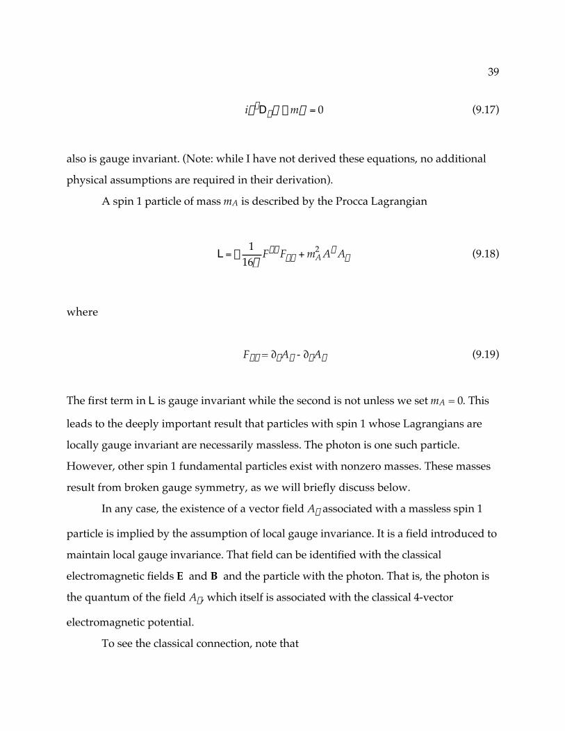
ig mDmy - my = 0 (9.17)

also is gauge invariant. (Note: while I have not derived these equations, no additional

physical assumptions are required in their derivation).

A spin 1 particle of mass mA is described by the Procca Lagrangian

†

L = -1

16pFmn Fmn + mA

2 Am Am (9.18)

where

Fmn = ∂mAn - ∂nAm (9.19)

The first term in L is gauge invariant while the second is not unless we set mA = 0. This

leads to the deeply important result that particles with spin 1 whose Lagrangians are

locally gauge invariant are necessarily massless. The photon is one such particle.

However, other spin 1 fundamental particles exist with nonzero masses. These masses

result from broken gauge symmetry, as we will briefly discuss below.

In any case, the existence of a vector field Am associated with a massless spin 1

particle is implied by the assumption of local gauge invariance. It is a field introduced to

maintain local gauge invariance. That field can be identified with the classical

electromagnetic fields E and B and the particle with the photon. That is, the photon is

the quantum of the field Am, which itself is associated with the classical 4-vector

electromagnetic potential.

To see the classical connection, note that

39

A'k = Ak + ∂k x(x) (9.20)

where k = 1, 2, 3, or, in 3-vector notation

A' = A + —x (9.21)

It follows that the 3-vector

B' = — x A' = — x A - — x —x = — x A = B (9.22)

is locally gauge invariant. Furthermore,

—•B = —•(— x A) = 0 (9.23)

Thus, B may be interpreted as the familiar classical magnetic field 3-vector; the above

equation is Gauss's law of magnetism, one of Maxwell's equations. The zeroth

component of the 4-vector potential,

†

¢ A o = Ao +∂x∂xo

(9.24)

can be written

†

¢ V = V -∂x∂t

(9.25)

40

which implies that the 3-vector

†

¢ E = -— ¢ V -∂ ¢ A ∂t

†

= -—V + —∂x∂t

-∂A∂t

-∂—x∂t

(9.26)

†

= -—V -∂A∂t

= E

is also locally gauge invariant. Furthermore,

†

— ¥ E +∂A∂t

Ê

Ë Á

ˆ

¯ ˜ = -— ¥ —V = 0 (9.27)

so

†

— ¥ E = -∂(— ¥ A)

∂t= -

∂B∂t

(9.28)

which is Faraday's law of induction, another of Maxwell's equations, with E interpreted

as the classical electric field.

Summarizing, we have found that the motion of a free charged particle is not

invariant under a local gauge transformation. However, we can make it invariant by

adding a term to the canonical momentum that corresponds to the 4-vector potential of

the electromagnetic field. Thus the electromagnetic force can be thought of as a

fictitious force that is introduced to preserve local gauge symmetry. Conservation of

charge follows from global gauge symmetry.

41

10. The Subnuclear Forces

The gauge transformation just described corresponds to a rotation in the abstract space

of the 4-momentum eigenstate, which is the state of any particle of constant

momentum. Here the transformation operator

U = exp(iq) (10.1)

can be trivially thought of as a1x1 matrix. The set of all such unitary matrices comprises

the transformation group U(1). The generators of the transformation, q, form a set of

1x1 matrices that, clearly, mutually commute. Whenever the generators of a

transformation group commute, that group is termed abelian. Electromagnetism is thus

an abelian gauge theory.

Recall from our discussion of angular momentum that the unitary operator

†

U = exp 12

is •qÊ

Ë Á

ˆ

¯ ˜ (10.2)

operates in the space of spin state vectors. In this case U is represented by a 2x2 matrix.

The set of all such matrices comprises the transformation group SU(2), where the prefix

S specifies that the matrices of the group are unimodular, that is, have unit determinant.

This follows from the fact that, for any matrix U,

U = exp(iA) (10.3)

we have

42

detU = exp(TrA) (10.4)

Since the Pauli matrices are traceless, detU = 1.

Following a procedure similar to what was done above for U(1), let us write

†

U = exp -12

igt ¥qÈ

Î Í

˘

˚ ˙ (10.5)

where the three components of t form a set of matrices identical to the Pauli spin

matrices and we use a different symbol just to avoid confusion with spin. While the spin

S = s/2 is a vector in familiar 3-dimensional space, t is a 3-vector in some more abstract

space we will call isospin space. The 3-vector T = t/2 is called the isospin or isotopic spin.

Global gauge invariance under SU(2) implies conservation of isospin. The quarks and

leptons of the standard model have T = 1/2. The quantity g is a constant analogous to

the electric charge that measures the strength of the interaction.

Once again it is important not to confuse isospin space with the 2-dimensional

subspace of the state vectors on which U operates. When the isospin space 3-vector x(x)

depends on the space-time (yet another space) position 4-vector x we once more have a

local gauge transformation. The generators being like angular momenta do not

mutually commute, so the transformation group is non-abelian. This type of non-abelian

gauge theory is called a Yang-Mills theory.

Let us attempt to make this clearer by rewriting U with indices rather than

boldface vector notion:

†

U = exp -12

igt kxk(x)

È

Î Í

˘

˚ ˙ (10.6)

43

where the repeated Latin index k is understood as summed from 1 to 3.

Encouraged by our success in obtaining the electromagnetic force from local

U(1) gauge symmetry, let us see what we can get from local SU(2) symmetry.

Following the U(1) lead, we define a covariant derivative

†

Dm = ∂m +12

igtkWmk (10.7)

where

†

Wmk are three 4-vector potentials analogous to to the electromagnetic 4-vector

potential Am. As before, the introduction of the fields

†

Wmk maintains local gauge

invariance. Or, we can say that local gauge invariance implies the presence of three 4-

vector potentials

†

Wmk . In the standard model, these are interpreted as the fields of the

weak interaction.

In quantum field theory, a particle is associated with every field, the so-called

quantum of the field. The spin and parity of the particle, JP , is determined by the

transformation properties of the field. The quantum of a scalar field has JP = 0+ ; a

vector field has JP = 1. For the electromagnetic field described by the potential Am, the

quantum is the photon. Since Am is a vector field, the photon has spin 1. It is a vector

gauge boson.

Similarly, the weak fields

†

Wmk will have three spin 1 particles as their

quanta—three vector gauge bosons W-, Wo, and W+ , where the superscripts specify the

electric charges of the particles. These can also be viewed as the three eigenstates of a

particle with isospin T = 1.

If the U(1) symmetry of electromagnetism and the SU(2) symmetry of the weak

interaction were perfect, we would see the photon and three W bosons above.

44

However, these symmetries are broken at the "low" energies at which most physical

observations are made, including those at the current highest energy particle

accelerators. This symmetry breaking leads to a mixing of the electromagnetic and

weak forces. Here, briefly, is how this comes about in what is called unified electroweak

theory.

The covariant derivative for electroweak theory (assumed, not derived) is

written

†

Dm = ∂m + ig1Y2

Bm + ig2t k2

Wmk (10.8)

where the U(1) field is called Bm and the constant g1 replaces the electric charge in that

term. The quantity Y is a constant called the hypercharge generator that can take on

different values in different applications, a detail that need not concern us here. The

SU(2) term includes a constant g2, the vector T = t/2, or isospin, and the vector field

†

Wmk,$k$= 1,"2,"3.

Neither B nor Wo , the quanta of the fields Bm and

†

Wmo , appear in experiments at

current accelerator energies. Instead, the particles that do appear are the photon and Z,

whose fields Am and Zm are mixtures of Bm and

†

Wmo . These together with the W+ and W-,

the quanta of the fields

†

Wmk,"k$=$1,"2, constitute the vector gauge bosons of the

electroweak sector of the standard model. Their mixing is also like a rotation, gauge

symmetry being broken in this case,

45

†

Am

Zm

Ê

Ë Á

ˆ

¯ ˜ =

cosqW sinqW-sinqW cosqW

Ê

Ë Á

ˆ

¯ ˜

Bm

Wmo

Ê

Ë Á Á

ˆ

¯ ˜ ˜ (10.9)

where the rotation angle qw is called the Weinberg (or weak) mixing angle. This parameter

is not determined by the theory and must be found from experiment. The current value

of sin2qw = 0.23115. The constants that determine the strength of the interaction are

g1 = e/cosqw g2 = e/sinqw (10.10)

where e is the unit electric charge.

As we have seen, the masses of gauge bosons are fundamentally zero. While the

photon is massless, the W± and Z bosons have large masses. These masses are shown to

arise from another symmetry-breaking process called the Higgs mechanism. The

symmetry-breaking is apparently spontaneous, that is, not determined by any known

deeper physical principle. Spontaneous symmetry breaking describes a situation, like

the ferromagnet, where the fundamental laws are symmetric and obeyed at higher

energy, but the lowest energy state of the system breaks the symmetry.

Moving beyond the weak interactions and SU(2), we have the strong

interactions and SU(3). In general, for SU(n) there are n2 - 1 dimensions in the subspace.

Let us add the new term to the previous ones that included the electroweak forces

†

Dm = ∂m + ig1Y2

Bm + ig2t k2

Wmk + ig3

la2

Gma (10.11)

where m = 0, 1, 2, 3 for the four dimensions of space-time, the repeated index k is

summed from 1 to 3 in the SU(2) term and the repeated index a is summed from 1 to 8

in the SU(3) term. The la are eight traceless 3x3 matrices analogous to the three Pauli

46

2x2 isospin matrices tk, and the

†

Gma are eight spin 1 fields analogous to the singlet field

Bm and the triplet field

†

Wmk . of the electroweak interaction. The gauge bosons in this case

are eight gluons. The symmetry is not broken, so they are massless. Global gauge

invariance under SU(3) implies the conservation of another quantity called color charge.

While there is much more to the standard model, this should suffice to illustrate

its basis in gauge symmetry and the importance of spontaneous broken symmetry.

11. General Relativity

General relativity can also be cast in the form of a gauge theory,[2] but to do so would

take us well beyond the mathematical scope of this paper which we have tried to limit

to the undergraduate level. However, we can outline how the principle of general

covariance leads to general relativity. Typical treatments emphasize the role of two

other principles, Mach's principle and the principle of equivalence. However, while Einstein

acknowledged Mach's influence on his thinking, it is not clear that Mach's principle

plays any significant part in deriving general relativity, especially since the principle

itself is ill-defined. The principle of equivalence between gravity and acceleration is

usually given great prominence, but that can also be seen as a consequence of the

principle of covariance.

Consider the equation of motion for a freely falling body in terms of a

coordinate system

†

y = (y0, y1, y2,y3 ) , where

†

yo = ict , falling along with the body. Since

†

dy = 0 ,

†

d2ydt2 = 0 (11.1)

Also,

47

†

d2yo

dt 2 = 0 (11.2)

Furthermore,

†

(dt )2 = (dt)2 -1c 2 dy 2

= (dt)2 (11.3)

Let us work in units where c = 1. We can write the above in 4-vector form,

†

d2ya

dt 2 = 0 (11.4)

This the 4-dimensional equation of motion for a body not acted on by any force.This

expresses the fact that a freely falling body experiences no external force.

Next, let us consider a coordinate system xa fixed to a second body such as the

earth, or any system that may be in relative acceleration. The equation of motion can be

transformed to that coordinate system as follows:

†

ddt

∂yr

∂xm

dxm

dt

Ê

Ë Á Á

ˆ

¯ ˜ ˜ = 0 (11.5)

from which, after some algebra,[3] we find

†

d2xl

dt 2 + Glmn

dxm

dtdxn

dt= 0 (11.6)

48

where

†

Glmn =∂xl

∂yr

∂2 yr

∂xm∂xn

(11.7)

is called the affine connection. An observer on earth witnesses a body accelerating

toward the earth and interprets it as the action of a "gravitational force." The principle of

equivalence thus merely defines gravity as the invisible force that produces the

observed acceleration. Glmn is a field that describes that force. Although Glmn has three

indices, it is not a tensor since it is not Lorentz invariant.

We can obtain the Newtonian picture in the limit of low speeds, dxk/dt ≈ 0. In

this case, dt = dt, d2xo/dt2 = 0, and

†

d2xk

dt 2 = Gkoo = gk (11.8)

for k = 1,2,3, where g = (g1, g2, g3) is the Newtonian field vector ("acceleration due to

gravity"). Thus, the Gkoo elements of the affine connection are just the Newtonian

gravitational field components in the limit of low speeds. Additional elements then are

needed to describe gravity at speeds near the speed of light.

The Newtonian field vector for any distribution of mass can be obtained from

the gravitational potential f which is in general a solution of Poisson's equation

†

— 2f = 4pGr (11.9)

where r is the mass density and g = -—f. For example, suppose that we have a point

49

mass m so that r(r) = md(r). Then,

†

f(r) = -Gm

r(11.11)

the familiar Newtonian result.

While the modified equation of motion (11.6) contains relativistic effects of

gravity, it is not covariant. It has a different form in the two reference frames. Einstein

sought to find equations to describe gravity that were covariant. He started with the

Poisson equation (11.9) above, which is noncovariant since r is the mass or energy

density and energy is the zeroth component of a 4-vector. Let us search for a covariant

quantity to replace density.

Suppose we have a dust cloud in which all the dust particles are moving

slowly, that is, with v << c, in some reference fame. Let the energy density in that

frame be ro . Let Eo be the rest energy of each particle (c = 1) and no be the number per

unit volume. Then,

ro = Eo no (11.12)

In some other reference frame the energy density will be

r = E n = g Eo g no = g2 ro (11.13)

where g is the Lorentz factor, E = g Eo, and n = g no. To see the latter, note that n =

dN/dV, where dN is the number of particles in the volume element dV, dNo = dN, and

dV = dVo/g from Fitzgerald-Lorentz contraction.

Note that r is not simply the component of a 4-vector because of the factor g2.

50

Rather it must be made part of a second-rank tensor. We can write

†

Tmn = rovmvn (11.14)

where vm is the 4-velocity of the cloud. Then, since vo = dt/dt = g,

†

Too = rovovo = g 2ro = r (11.15)

Tmn is the energy-momentum tensor, or stress-energy tensor. The other components

comprise energy and momentum flows in various directions: Toi is the energy flow per

unit area in the i-direction, that is, a heat flow; Tii is the flow of momentum component i

per unit area in their direction, the pressure across the i plane; Tij is the flow of

momentum component i per unit area in the j-direction, the viscous drag across the j-

plane; Tio is the density of the i component of momentum.

Einstein thus wrote, as the covariant form of Poisson's equation,

†

Gmn = -8pGTmn (11.16)

where G is Newton's constant and the factor is chosen so that we get Poisson's equation

in the Newtonian limit. Since the energy-momentum tensor Tmn is covariant, the

quantity Gmn is also a covariant tensor field.

By associating Gmn with the energy-momentum tensor, Einstein was using, at

most, a very weak form of Mach's principle that was much earlier proposed by Leibniz.

Leibniz had objected to Newton's notion of an absolute space with respect to which

bodies accelerate and argued that at least another body must be present for space and

time concepts to be useful.[4]

51

In what has become the standard model of general relativity, Einstein related

Gmn to the curvature of space-time in a non-Euclidean geometry. In non-Euclidian

geometry, the proper distance between two points in space-time is

†

(Ds)2 = Dx mgmn Dxn (11.17)

where gmn is the metric tensor.

Einstein assumed that Gmn is a function of gmn and its first and second derivatives.

In its usual form, Einstein's field equation is given as

†

Rmn -12

gmn R + Lgmn = -8pGTmn (11.18)

where Rmn and R are contractions of the rank four Riemann curvature tensor. To see the

explicit forms of these quantities, consult any textbook on general relativity.

The quantity L is the infamous cosmological constant. It is often reported in the

media and in many books on cosmology that the cosmological constant was a "fudge

factor" Einstein introduced to make things come out the way he wanted. Perhaps that

was his motivation, but the fact is that unless one makes further assumptions, a

cosmological constant is required by Einstein's equations of general relativity and

should be kept in the equations until some principle is found that shows it to be zero.[5]

For many years the measurements of the cosmological constant gave zero within

measuring errors, but in the past two decades Einstein's fudge factor has resurfaced

again in cosmology.

12. Conclusions

The sophisticated reader who at least has glanced at the equations in this paper will

52

recognize them as very familiar. Almost every one can be found in standard textbooks.

What has been attempted here is to show that those equations do not follow from very

unique or very surprising physical properties of the universe. Rather, they arise from

the very simple notion that whatever mathematical "laws" you write down to describe

measurements, your equations cannot depend on the origin or direction of the

coordinate systems you define in the space of those measurements or the space of the

functions used to describe those laws. That is, they cannot reflect any privileged point of

view. Except for the complexities that result from spontaneously broken symmetries,

the laws of physics may be the way they are because they cannot be any other way. Or,

at least they may have come about the simplest way possible. Table 11.1 summarizes

these conclusions.

Acknowledgements

Special thanks to Brent Meeker and other members of the avoid-L discussion group for

their help with this manuscript.

Table 1. The laws and other basic ideas of physics and their origin.

Law/idea of Physics OriginConservation of momentum Space translation symmetryConservation of angular momentum Space rotation symmetryConservation of energy(First law of thermodynamics) Time translation symmetryNewton's 1st Law of Motion Conservation of momentum

(space translation symmetry)Newton's 2nd Law of Motion Definition of forceNewton's 3rd Law of Motion Conservation of momentum

(space translation symmetry)Second law of thermodynamics Statistical definition of the arrow of timeSpecial relativity Space-time rotation symmetryInvariance of speed of light Space-time rotation symmetry

53

General relativity Principle of covarianceQuantum time evolution(time-dependent Schrödinger equation) Global gauge invarianceQuantum operator differential forms Global gauge invarianceQuantum operator commutation rules Global gauge invarianceQuantization of action Global gauge invarianceQuantization rules for angular momenta Global gauge invarianceMaxwell's equations of electromagnetism Local gauge invariance under U(1)Quantum Lagrangians for particles in presence of electromagnetic field Local gauge invariance under U(1)Conservation of electric charge Global gauge invariance under U(1)Masslessness of photon Local gauge invariance under U(1)Conservation of weak isospin Global gauge invariance under SU(2)Electroweak Lagrangian Mixing of U(1) and S(2) local gauge

symmetries (spontaneous symmetry breaking)

Conservation of color charge Global gauge invariance under SU(3)Strong interaction Lagrangian Local gauge invariance under SU(3)Masslessness of gluon Local gauge invariance under SU(3)Structure of the vacuum (Higgs particles) Spontaneous symmetry breakingDoublet structure of quarks and leptons Conservation of weak isospin

(global gauge invariance under SU(2))Masses of particles Higgs mechanism

(spontaneous symmetry breaking)

54

References55

1. E. Noether, Nachr. d. König. Gesellsch. d. Wiss. zu Göttingen, Math-phys. Klasse,235 (1918), p. 7; English translation M. A. Travel, Transport Theory and StatisticalPhysics 1(3), 183 (1971). See also Nina Byers, in Proceedings of the IsraelMathematical Conference 12 (1999). Online athttp://www.physics.ucla.edu/~cwp/articles/noether.asg/noether.html. Thiscontains links to Noether's original paper including an English translation. 2. F. W. Hehl, J. D. McCrea, E. W. Mielke and Y. Ne'eman, Phys. Rep. 258, 1 (1995).

3. Steven Weinberg, Graviation and Cosmology: Principles and Applications of theGeneral Theory of Relativity (New York London Sydney Toronto: John Wiley &Son, 1972), p. 102.

4. Jennifer Trusted, Physics and Metaphysics: Theories of Space and Time, Paperbackedition (London and New York: Routledge, 1994), p. 90.

5. Weinberg, Gravitation and Cosmology, pp. 613-6.