where and how should we put more salt - wolf dynamics · tips and tricks in openfoam® where and...

Tips and tricks in OpenFOAM®

Where and how should we

put more salt

1

… and as this is kind of a cooking recipe, it comes with a

small warning


• What I am about to show you is based on my personal experience.

• To draw these kind of conclusions or observations, I conducted hundreds of

numerical experiments, under different conditions, with different meshes

(from good quality meshes to bad quality meshes with different cell types),

and different physics and models involved.

• Most important of all, before starting this long road, I got familiar with the

theory behind the FVM and CFD, the physics behind what I was doing, and

OpenFOAM® source code.

• At this point, I highly advise you to conduct similar numerical experiments

and draw your own conclusions.

• Please, use these slides as a reference only. I am not responsible

for your failures and mistakes.

2


Our vertical workflow• Do you remember this vertical workflow? I hope so.

• Everything starts with the geometry. So in order to

get a good mesh, you need a good geometry.

• When it comes to geometry generation, the only rule

you should keep in mind is that by the end of the day

you should get a unique clean and watertight

geometry.

• Geometry defeaturing can made your life easier. Do

not fool yourself, if you have no constraints avoid

sharp angles.

• And as for the mesh concerns, try to keep the

skewness, orthogonality, aspect ratio, and growth rate

low.

• No need to say that if you have a bad geometry, is

likely probable that your mesh will be bad as well.

• Always remember: good mesh – good results.3

MESH GENERATION

CASE SETUP AND SOLUTION

POST-PROCESSING

GEOMETRY GENERATION


### OPENFOAM ###

# source $HOME/OpenFOAM/OpenFOAM-1.6-ext/etc/bashrc

# source $HOME/OpenFOAM/OpenFOAM-1.6-ext.GPU/etc/bashrc

# source $HOME/OpenFOAM/OpenFOAM-2.1.1/etc/bashrc

# source $HOME/OpenFOAM/OpenFOAM-2.3.0-debug/etc/bashrc

# source $HOME/OpenFOAM/OpenFOAM-2.3.x/etc/bashrc


source $HOME/OpenFOAM/OpenFOAM-3.0.x/etc/bashrc

### OPENFOAM ###

OpenFOAM® shell environment

• You can have as many versions of OpenFOAM® as you like living together. You just

need to source the right environment variables. For instance, on my workstation I have seven versions living together. This is how my .bashrc file looks like,

4


### OPENFOAM ###








### OPENFOAM ###


• If at any time I want to use a different version of OpenFOAM®, I just source the right

OpenFOAM® environment variables. For instance if I want to switch from version 2.3.x to version 3.0.x, I modify my .bashrc as follows,

### OPENFOAM ###








### OPENFOAM ###

Old .bashrc New .bashrc

• Then open a new terminal, and you can start using the new version. You can also

have two different versions of OpenFOAM® running together at the same time in

different terminals.

• You can also use aliases to source the OpenFOAM® version.5



• You can also use aliases to source the OpenFOAM® version. This is how my .bashrc file looks like,

alias of23x='source /home/joegi/OpenFOAM/OpenFOAM-2.3.x/etc/bashrc'



alias fe31='source /home/joegi/foam/foam-extend-3.1/etc/bashrc'

• If I want to start using OpenFOAM® version 3.0.x, I just type in the terminal of3x.

• You can also have two different versions of OpenFOAM® running together at the

same time in different terminals.

6



• When switching from one OpenFOAM® version to another one, it is highly advisable

to clear as many OpenFOAM environment settings as possible, to do so you can use the script unset.sh. In the terminal type:

• $> unset

• Be careful, there may be more than one unset.sh script. The OpenFOAM® specific

script is located in the directory $WM_PROJECT_DIR/etc/config.

• You can also use the alias wmUNSET, which is set in the OpenFOAM® environment

variables. Remember, you can type alias in the terminal window to see all the

aliases available.

• In the directory $WM_PROJECT_DIR/etc/config, you will also find many useful

scripts. For instance, you can take a look at the script aliases.sh, in this script you

will find all the aliases defined in OpenFOAM®

7


Looking for information in OpenFOAM® source code

• To locate files you can use the find command. For instance, if you want to locate a

file that contains the string fvPatch in its name you can proceed as follows,

• $> find $FOAM_SRC -name "*fvPatch*"

This command will locate the files containing the string "*fvPatch*" in the

directory $FOAM_SRC

• If you want to find a string inside a file, you can use the command grep

• $> grep -r -n LES $FOAM_SOLVERS

This command will look for the string LES in all files inside the directory$FOAM_SOLVERS. The argument-r means recursive and -n will output the line

number.

8


• As you might already know, there are a gazillion dictionaries in OpenFOAM®. The

easiest way to find all of them is to do a local search in the installation directory as

follows,

• For instance, if you are interested in finding all dictionary files that end with the "Dict" word in the tutorials directory, in the terminal type:

• $> find $FOAM_TUTORIALS -name "*Dict"

• $> find $FOAM_TUTORIALS -iname "*dict"


9


• A few more advanced commands to find information in your OpenFOAM® installation.

• To find which tutorial files use the boundary condition "slip":

• $> find $FOAM_TUTORIALS -type f | xargs grep -sl 'slip'

• To find where the source code for the boundary condition "slip" is located:

• $> find $FOAM_SRC -name "*slip*"

• To find what applications do not run in parallel

• $> find $WM_PROJECT_DIR -type f | xargs grep -sl 'noParallel'

• Remember, OpenFOAM® understand REGEX syntax.


10


OpenFOAM® Doxygen documentation

• The best source of information is the source code and the Doxygen documentation.

• The $WM_PROJECT_DIR/doc directory contains the Doxygen documentation of

OpenFOAM®.

• Before using the Doxygen documentation, you will need to compile it. To compile the

Doxygen documentation, from the terminal:

• $> cd $WM_PROJECT_DIR

• $> ./Allwmake doc

Note: You will need to install doxygen and graphviz/dot

• After compiling the Doxygen documentation you can use it by typing:

• $> firefox file://$WM_PROJECT_DIR/doc/Doxygen/html/index.html

• The compilation is time consuming. 11


Intensive IO

• If you are doing intensive IO or running big cases, I highly advise you to save the

solution in binary format. When using binary format, the IO is a way much faster and

the output files use less space.

• Remember, you can get a performance gain when you save in binary format as you

minimize any requirement for parsing.

• If OpenFOAM® binary format is not good enough for you, you can try another format.

For instance you can use HDF5 format with OpenFOAM®.

http://openfoamwiki.net/index.php/Contrib/IOH5Write

12

http://openfoamwiki.net/index.php/Contrib/IOH5Write


Intensive IO

• Know your hardware, intensive IO can slow-down your computations or crash your

system, even the most powerful supercomputers.

• For big simulations, most of the times the bottleneck is the IO.

• No need to say that eventually you will run out of space if you are working with big

files.

• One naive solution to the IO bottleneck and big datasets space, do not save your

solution very often. But be careful, at least save your solution before stopping your

solution or reaching the job maximum time.

13


Running in a cluster

• Best advice, familiarize with your hardware.

• Do not get overwhelm when running in a cluster. Running OpenFOAM® in a cluster

is not different from running in your workstation or portable computer. The only

difference is that you need to schedule your jobs.

• Depending on the system current demand of resources, the resources you request

and your job priority, sometimes you can be in queue for hours, even days, so be

patient and wait for your turn.

• Consequently, remember to always double or triple check your scripts. It will be a

waste of time if after two days in queue, your simulation did not start because there

were errors in your scripts.

• For those running on fancy clusters, such as blue gene supercomputers, I have found

a processor limit of 512, after that is quite difficult to get any improvement.

• Also, the IO is really time consuming.

14


Running in a cluster

• By the way, I know it looks super cool, but try to avoid spaces or funny characters

when naming directories and files, specially if you run in clusters. e.g.:

• my dictionary.dict instead use my_dictionary.dict

• #my_file;txt instead use my_file.txt

• my/solution!!! instead use my_solution

• working@home instead use working_at_home

• This is a dir instead use this_is_a_dir

• directory+1! instead use directory_1

• Also, I do not recommend you to use underscore as the first character when naming your files or directories

• _my_dir instead use my_dir

• _my_file instead use my_file

15


OpenFOAM® mesh quality and checkMesh utility

• Before running a simulation remember to always check the mesh quality using the checkMesh utility.

• Remember, good quality meshes are of paramount importance to obtain accurate

results.

• checkMesh will also check for topological errors.

• Have in mind that topological errors must be repaired.

• You will be able to run with mesh quality errors (such as skewness, aspect ratio,

minimum face area, and non-orthogonality), but they will severely tamper the solution

accuracy and can made the solver run super slow or even blow-up.

• In my personal experience, I have found that OpenFOAM® is very picky when it comes to mesh quality. So if checkMesh is telling you that the mesh is bad, you

better correct those errors.

• Unfortunately, to correct mesh quality errors you will have to remesh the geometry.

16


• If for any reason checkMesh finds errors, it will give you a message and it will tell you

what check failed.

• It will also write a set with the faulty cells, faces, and/or points. These sets are saved in the directory constant/polyMesh/sets/

• If at any point you want to visualize the failed faces/cells/points you will need to convert them to VTK format using the utility foamToVTK.

• At the end, foamToVTK will create a directory named VTK, where you will find the

failed faces/cells/points in VTK format. At this point you can use paraFoam or

paraview to visualize the failed sets.

• I want to emphasize the fact that you will be able to run with mesh quality

errors such as skewness, aspect ratio, minimum face area, and non-

orthogonality.

• However, they will severely tamper the solution accuracy and can made the

solver explode.

17



• If you want to know the quality metrics hard-wired in OpenFOAM®, just read the file $WM_PROJECT_DIR/src/OpenFOAM/meshes/primitiveMesh/primitiveMesh

Check/primitiveMeshCheck.C. Their maximum (or minimum) values are defined

as follows:

• By the way, if you are not happy with these values, you can just change them and

voila, your quality problems are solved (I am kidding of course).

18


36 Foam::scalar Foam::primitiveMesh::closedThreshold_ = 1.0e-6;

37 Foam::scalar Foam::primitiveMesh::aspectThreshold_ = 1000;

38 Foam::scalar Foam::primitiveMesh::nonOrthThreshold_ = 70; // deg

39 Foam::scalar Foam::primitiveMesh::skewThreshold_ = 4;

40 Foam::scalar Foam::primitiveMesh::planarCosAngle_ = 1.0e-6;


OpenFOAM® mesh quality and renumberMesh utility

• Before running a simulation, I highly recommend you to use the renumberMesh

utility. This utility will renumber the mesh to minimize its bandwidth, in other words, it

will make the linear solver run faster (at least for the first time-steps)

• Summarizing, before running a simulation remember to always check the mesh quality using checkMesh and then reduce the mesh bandwidth by using the

renumberMesh. This is a good standard practice, I always do it (at least for big

meshes).

• Before running a simulation, try to always get a good quality mesh. Remember,

garbage in – garbage out. Or in a positive way, good mesh – good results.

19


Boundary conditions

• Boundary conditions should be physically realistic. They must represent the physics

involved.

• Minimize grid skewness, non-orthogonality, growth rate, and aspect ratio near the

boundaries. You do not want to introduce diffusion errors early in the simulation,

specially close to the inlets.

• Get a good quality mesh at the boundaries.

• Remember, for each single variable you are solving you need to specify a boundary

condition.

• Try to avoid large gradients in the direction normal to the boundaries near inlets and

outlets. That is to say, put your boundaries far away from where things are

happening.

• Do not force the flow at the outflow, use a zero normal gradient for all flow variables

except pressure. The solver extrapolates the required information from the interior.

• Be careful with backward flow at the outlets (flow coming back to the domain) and

backward flow at inlet (reflection waves), they require special treatment.20


Initial conditions

• First at all, a good initial condition can improve the stability and convergence rate. On

the other hand, unphysical boundary conditions can slow down the convergence rate

or can cause divergence.

• As for boundary conditions, for each single variable you are solving you need to

specify initial conditions.

• When it is possible, use potentialFoam to get an initial solution. It is computational

inexpensive.

• potentialFoam can also give you an idea of the sensitivity of the mesh quality.

• You can also get a computational inexpensive solution on a coarse mesh and then

interpolate it to a fine mesh. This will be a very good initial solution only if the solution

in the coarse mesh is acceptable.

• By the way, do not forget to use a good quality coarse mesh.

• Use mapFields to map the solution from a coarse mesh to a finer mesh. It also

works the other way around, but I do not see any reason to proceed in this way.

21


Initial conditions

• If you are using a turbulence model, you can initialize the velocity and pressure fields

from the solution obtained from a laminar case.

• If you are running an unsteady simulation and if the initial transient is of no interest,

you can initialize your flow using the solution obtained from a steady simulation.

• Always try to get initial conditions that are close to the solution (I know this is difficult

to achieve as we do not know the solution, if we knew the solution we would not have

a job).

• I want to remind you again, initial conditions should be physically realistic.

22


Starting and running a simulation

• Remember, you can change the parameters in the dictionaries controlDict,

fvSchemes and fvSolution on-the-fly. But you will need to set the keyword

runTimeModifiable to yes in the controlDict dictionary.

• When starting a simulation and if the initial transient is of no interest, you can start the

simulation by using a high value of viscosity (low Reynolds number), and as the

simulation runs you can change the value until you reach the desired value.

• If you are working with high Reynolds numbers and you do not like the trick of

increasing the viscosity, you can get a very good initial solution using an Euler solver

with upwind.

• You can also start the simulation by using a first order scheme and then switch to a

high order scheme.

23


• You can also change the convergence criterion of the linear solvers on the fly.

• For instance, you can start using a not so tight convergence criterion with a robust

numerical scheme, and as the simulation runs you can tighten the convergence

criterion to increase the accuracy.

• When the simulation starts I usually use more correctors steps (for PISO and PIMPLE

methods), and as the solution advance or stabilizes I decrease the number of

corrector steps, but I always use at least one corrector step.

• Remember to always check the time step continuity errors. This number should be

small (negative or positive), if it increases in time for sure something is wrong.

• If you want to know how the continuity errors are computed just type in the terminal find $FOAM_SRC –iname *continuity*, and open any of the files.

24

Starting and running a simulation


Discretization schemes

• Never get a final solution using first order schemes. They are too diffusive, which

means they will under predict the forces and smear the gradients. In the other side,

first order schemes are extremely robust, so you might be tented to use them as they

will always give you a solution.

• You can start using a first order scheme, and then switch to a high order scheme.

Remember, you can change the parameters on the fly.

• This means, start robustly and end with accuracy.

• By the way, an accurate numerical scheme needs a good quality mesh.

• Bad quality meshes will add numerical oscillations and reduce the accuracy of the

numerical solution.

25


• If you have a good mesh and a good initial solution, you can start immediately with

a high order scheme, but be careful, remember to always check the stability of the

solution.

• If at one point your solution starts to oscillate, you can switch to upwind and let the

simulation stabilize, then you can switch back to high order accuracy.

• Have in mind that this behavior is telling you that something is happening so you

better adjust other parameters, such as, solver tolerances, non-orthogonal

corrections, number of correctors, gradient discretization and so on.

• Try to always use a good quality mesh. Avoid the GIGO syndrome.

• In the next slides I will show you how I usually setup the discretization schemes.

26

Discretization schemes


Discretization schemes – Convective terms

• A robust numerical scheme but too diffusive (first order accurate),

divSchemes

{

div(phi,U) Gauss upwind;

div(phi,omega) Gauss upwind;

div(phi,k) Gauss upwind;

div((nuEff*dev2(T(grad(U))))) Gauss linear;

}

27


• An accurate and stable numerical scheme (second order accurate),

divSchemes

{

div(phi,U) Gauss linearUpwind grad(U);

div(phi,omega) Gauss linearUpwind default;

div(phi,k) Gauss linearUpwind default;


}

28



• An even more accurate but oscillatory scheme (second order accurate),

divSchemes

{

div(phi,U) Gauss linear;




}

29


laplacianSchemes

{

default Gauss linear limited ;

}


• For the discretization of the diffusive terms, you can use a fully orthogonal scheme,

Discretization schemes – Diffusive terms

laplacianSchemes

{

default Gauss linear corrected;

}

• You can also use a scheme that uses a blending between a fully orthogonal scheme

and a non-orthogonal scheme,

30


• The method you use highly depends on the quality of the mesh.

• For meshes with low non-orthogonality you can use the corrected scheme or the

limited 1 scheme.

• For meshes with high non-orthogonality you can use the limited scheme. The higher the non-orthogonality the lower the value of the blending factor .

0 1• Good quality mesh

• Orthogonal correction

• Unbounded on low quality meshes

• Bad quality mesh

• Non-orthogonal correction

• Bounded on low quality meshes

31



• An accurate numerical scheme on orthogonal meshes (this is a very good quality

mesh with uniform cell size, this is what we want),

laplacianSchemes

{

default Gauss linear orthogonal;

}

snGradSchemes

{

default orthogonal;

}

32



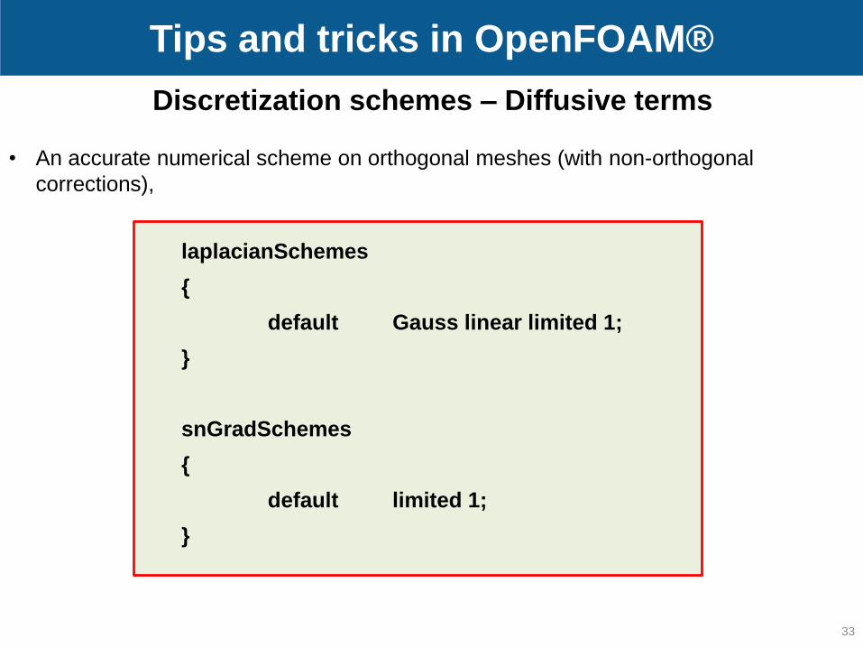
• An accurate numerical scheme on orthogonal meshes (with non-orthogonal

corrections),

laplacianSchemes

{

default Gauss linear limited 1;

}

snGradSchemes

{

default limited 1;

}

33



• A less accurate numerical scheme valid on non-orthogonal meshes (with non-

orthogonal corrections),

laplacianSchemes

{

default Gauss linear limited 0.5;

}

snGradSchemes

{

default limited 0.5;

}

34



• Let’s talk about the gradSchemes, this entry defines the way we compute the

gradients.

• The gradients can be computed using the Gauss method or the least squares

method. The keywords are:

• Gauss linear;

• leastSquares;

• In practice, the leastSquares method is more accurate, however, I have found that it

tends to be more oscillatory on tetrahedral meshes.

Discretization schemes – Gradient terms

35


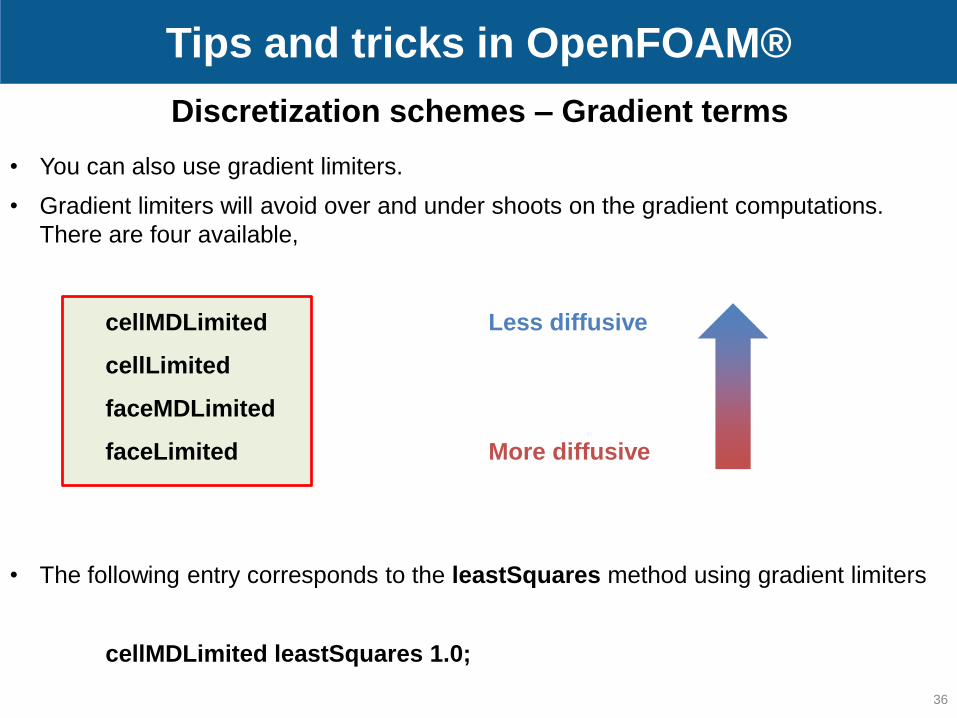
• You can also use gradient limiters.

• Gradient limiters will avoid over and under shoots on the gradient computations.

There are four available,

cellMDLimited Less diffusive

cellLimited

faceMDLimited

faceLimited More diffusive

• The following entry corresponds to the leastSquares method using gradient limiters

cellMDLimited leastSquares 1.0;

36



• Gradient limiters avoid over and under shoots on the gradient computations.

• The gradient limiter implementation in OpenFOAM®, uses a blending factor .

gradSchemes

{

default cellMDLimited Gauss linear ;

}

0 1Stability

Limiter onAccuracy

Limiter off 37



Discretization schemes – How to choose the schemes

• If after checking the mesh quality, the non-orthogonality is higher than 80, I prefer to

redo the mesh and improve the quality.

• By the way, if you are running LES simulations, do not even think about running in

highly non-orthogonal meshes. Better spend more time in getting a good quality

mesh, maybe with non-orthogonality less than 70.

• Do not try to push too much the numerical scheme on highly non-orthogonal meshes.

You already know that the quality is low, so this highly influence the accuracy and

stability of the solution. Specially the gradient computations.

• I do not like to run simulations on highly orthogonal meshes, but if I have to, I often

use the following numerical scheme.

38


• Non-orthogonality more than 85. I do not waste my time. I prefer to go back and get a

better mesh. But if you want, you can try something like this,

gradSchemes

{

default faceLimited leastSquares 1.0;

grad(U) faceLimited leastSquares 1.0;

}

divSchemes

{




div((nuEff*dev(T(grad(U))))) Gauss linear;

}

laplacianSchemes

{


}

snGradSchemes

{


}

39



• Non-orthogonality between 70 and 85

gradSchemes

{

default cellLimited leastSquares 1.0;

grad(U) cellLimited leastSquares 1.0;

}

divSchemes

{





}

laplacianSchemes

{


}

snGradSchemes

{


}

40




gradSchemes

{

default cellMDLimited Gauss linear 0.5;

grad(U) cellMDLimited Gauss linear 0.5;

}

divSchemes

{





}

laplacianSchemes

{


}

snGradSchemes

{


}

41




gradSchemes

{

default cellMDLimited Gauss linear 0.5;

grad(U) cellMDLimited Gauss linear 0.5;

}

divSchemes

{





}

laplacianSchemes

{


}

snGradSchemes

{


}

42



• I guess at this point you know how to adjust the numerical scheme for meshes with

non-orthogonality less than 40.

• Additionally, I also change the number of non-orthogonal corrections.

• Non-orthogonality between 70 and 85:

nNonOrthogonalCorrectors 3;

• Non-orthogonality between 50 and 70:


• Non-orthogonality less than 50:


• I always like to do at least one non orthogonal correction.43



Under-relaxation factors

• Because of the non-linearity of the equations being solved, it is necessary to control

the change of . This is achieved by under-relaxation as follows,

here is the relaxation factor,

• In plain English, this means that the new value of the variable depends upon the

old value, the computed change of , and the under-relaxation factor .

Means under-relaxation. This will slow down the convergence

rate but increases the stability.

Means no relaxation at all. We simple use the predicted value of .

Means over-relaxation. It can sometimes be used to accelerate

convergence rate but will decrease the stability.

44


• Under-relaxation factors are typical of steady solvers using the SIMPLE method.

• To find out what are and how to change the under-relaxation factors requires

experience and understanding.

• In general, under-relaxation factors are there to suppress oscillations.

• Small under-relaxation factors will significantly slow down convergence. Sometimes

to the extent that the user thinks the solution is converged when in really is not.

• The recommendation is to always use under-relaxation factors that are as high as

possible, without resulting in oscillations or divergence.

45



• I highly recommend you to use the default under-relaxation factors.

• If you have to change the under-relaxation factors, start by decreasing the values of

the under-relaxation factors in order to improve the stability of the solution.

• Remember, low under-relaxation factors will slow down the solver while high under-

relaxation factors will speed up the computation, but you will give up stability.

• In order to find the optimal under-relaxation factors for your case, it will take some trial

and error.

46


• These are the under-relaxation factors I often use (which by the way are the

commonly used).

relaxationFactors

{

p 0.3;

U 0.7;

k 0.7;

omega 0.7;

}

• According to the physics involved you will need to add more under-relaxation factors.

• If you do not define the new under-relaxation factors, they will be set to 1.0 by default.


47



0 1

relaxationFactors

Stability

Velocity

48



Linear solvers

• The linear solvers are defined in the fvSolution dictionary. You will need to define

a solver for each variable you are solving.

• The solvers can be modified on the fly.

• The GAMG solver (generalized geometric-algebraic multigrid solver), can often be the

optimal choice for solving the pressure equation. However, I have found that when

using more than 1024 processors is better to use Newton-Krylov type solvers.

• When solving multiphase problems, I have found that the GAMG solver might give

problems when running in parallel, so be careful. The problem is mainly related to

nCoarsestCells keyword, so usually I have to set a high value of cells (in the order

1000).

• The utility renumberMesh can dramatically increase the speed of the linear solvers,

specially during the firsts iterations.

• I usually start by using a not so tight convergence criterion and as the simulation runs,

I tight the convergence criterion.

49


• These are the linear solvers I often use.

• For the pressure equation I usually start with a tolerance equal to 1e-5 and relTol

equal to 0.01. After a while I change these values to 1e-6 and 0.001 respectively.

p

{

solver GAMG;

tolerance 1e-5;

relTol 0.01;

smoother GaussSeidel;

nPreSweeps 0;

nPostSweeps 2;

cacheAgglomeration on;

agglomerator faceAreaPair;

nCellsInCoarsestLevel 1000;

mergeLevels 1;

}

50

Linear solvers





p

{

solver GAMG;

tolerance 1e-6;

relTol 0.001;


nPreSweeps 0;

nPostSweeps 2;




mergeLevels 1;

}

51

Linear solvers



• If I do not use the GAMG solver for the pressure, I often use the PCG solver.



• If the speed of the solver is too slow, I change the convergence criteria to 1e-4 and

relTol equal to 0.05. I usually do this during the first iterations.

p

{

solver PCG;

preconditioner DIC;

tolerance 1e-4;

relTol 0.05;

}

52

Linear solvers



• For the velocity equation I always use a tolerance equal to 1e-8 and

relTol equal to 0.0

U

{

solver PBiCG;

preconditioner DILU;

tolerance 1e-8;

relTol 0.0;

}

53

Linear solvers


• I like to set the minimum number of iterations to three, especially for the pressure.

• If your solver is doing too many iterations, you can set the maximum number of

iterations. But be careful, if the solver reach the maximum number of iterations it will

stop, we are talking about unconverged iterations.

• You can set the maximum number of iterations specially during the first time-steps

where the solver takes longer.

• I use minIter and maxIter on symmetric and asymmetric matrix solvers.

p

{

solver PCG;

preconditioner DIC;

tolerance 1e-4;

relTol 0.01;

minIter 3;

maxIter 100;

}

54

Linear solvers


• The default option is the conventional segregated solution. That is, you first solve for

velocity component X, then velocity component Y, and finally velocity component Z.

• You can get some improvement in terms of stability and turn around time by using the

coupled matrix solver for vectors and tensors, i.e., if you are solving the velocity field,

you solve all the velocity components at once.

• To select the coupled solver you need to use the keyword coupled in the fvSolution dictionary.

• In the coupled matrix solver you set tolerance as a vector (absolute and relative)

U

{

type coupled;

solver cPBiCCCG;

preconditioner DILU;

tolerance (1e-08 1e-08 1e-08);

relTol (0 0 0);

minIter 3;

}55

Linear solvers


• Remember, you must do at least one corrector step when using PISO solvers.

• When you use the PISO and PIMPLE solvers, you also have the option to set the

tolerance for the final corrector step (.*Final).

• By proceeding in this way, you can put all the computational effort only in the last

corrector step (.*Final).

pFinal

{

solver GAMG;

tolerance 1e-06;

relTol 0.0;


nPreSweeps 0;

nPostSweeps 2;




mergeLevels 1;

}

56

Linear solvers


• By proceeding in this way, you can put all the computational effort only in last

corrector step (.*Final).

• For all the intermediate corrector steps, you can use a more relaxed convergence

criterion.

• For example, you can use the following solver and tolerance criterion for all the

intermediate corrector steps (p), then in the final corrector step (pFinal) you tight the

solver tolerance.

p

{

solver GAMG;

tolerance 1e-05;

relTol 0.05;


nPreSweeps 0;

nPostSweeps 2;




mergeLevels 1;

}

pFinal

{

solver GAMG;

tolerance 1e-06;

relTol 0.0;


nPreSweeps 0;

nPostSweeps 2;




mergeLevels 1;

}57

Linear solvers


Transient simulations and time-step selection

• Remember, the fact that we are using an implicit solver (unconditionally stable), does

not mean that we can choose a time step of any size.

• The time-step must be chosen in such a way that it resolves the time-dependent

features and it maintain the solver stability.

58


• In my personal experience, I have been able to go up to a CFL = 5.0 while

maintaining the accuracy. To achieve this I had to increase the number of corrector

steps in the PIMPLE solver, decrease the under-relaxation factors and tightening the

convergence criteria; and this translates into a higher computational cost.

• I have managed to run with CFL numbers up to 40, but this highly reduces the

accuracy of the solution. Also, is quite difficult to maintain the stability of the solver.

• As I am often interested in the unsteadiness of the solution, I usually use a CFL

number not larger than 1.0.

59



• If accuracy is the goal (e.g., predicting forces), definitively use a CFL less than 1.0.

• If you are doing LES simulations, I highly advice you to use a CFL less than 0.6 and if

you can afford it, less than 0.3

• If you are doing LES or you are interested in the accurate prediction of forces,

definitely you need high quality meshes, preferable made of hexahedral elements.

• I usually use the PIMPLE solver. In the PIMPLE solver you have the option to limit

your time-step to a maximum CFL number, so the solver automatically choose the

time-step. This is a very cool feature.

• In the PISO solver you need to give the time-step size. So basically you need to

choose your time-step so it does not exceed a target CFL value.

60



• You can easily modify the PISO solver so it automatically choose the time-step

according to a maximum CFL number, you just need to add one line of code.

• Remember, setting the keyword nOuterCorrectors equal to 1 in the PIMPLE solver

is equivalent to use the PISO solver.

• The PIMPLE solver is a solver specially formulated for large time-steps. So in order

to increase the stability you will need to add more corrector steps (nOuterCorrectors

and nCorrectors).

• Remember, you need to do add least one nCorrector when using the PISO method.

• A smaller time-step may be needed in the first iterations to maintain solver stability.

Have in mind that the first time steps may take longer to converge, do not be alarmed

of this behavior, it is perfectly normal.

61



• If you are interested in the initial transient, you should start using a high order

discretization scheme, with a tight convergence criterion, and the right flow properties.

• If you start from an approximate initial solution obtained from an steady simulation,

the initial transient will not be accurate.

• If the solution is not converging or is taking too long to converge, try to reduce your

time-step.

• If you use the first order Euler scheme, try to use a CFL number less than 1.0 and

preferably in the order of 0.6-0.8, this is in order to keep temporal diffusion to a

minimum. Yes, numerical diffusion also applies in time.

62



• In order to speed up the computation and if you are not interested in the initial

transient, you can start using a large time-step (high CFL).

• When you are ready to sample the quantity of interest, reduce the time-step to get a

CFL less than one and let the simulation run for a while before doing any sampling.

• My recommendation is to always monitor your solution, and preferably use the

PIMPLE solver with no under-relaxation.

• When using the PIMPLE or PISO solver (with maximum CFL feature enable), the

solver will use as a time-step for the first iteration the value set by the keyword deltaTin the controlDict dictionary. So if you set a high value, is likely that the solver will

explode.

63



• My advice is to set a low deltaT and then let the solver gradually adjust the time-step

until the desired maximum CFL is reached.

• Some fancy high order numerical schemes (such as the vanLeer, vanAlbada,

superbee, MUSCL, OSPRE – cool names no – ), are hard to start. So it is better to

begin with a small time-step and increase it gradually.

• And by small time-step I mean a time-step that will give you a CFL about 0.1.

• Remember, you can change the temporal discretization on the fly. As for the spatial

discretization, first order schemes are robust and second order schemes are

accurate.

64



• The temporal discretization schemes are set in the fvSchemes dictionary. To select

the schemes you need to use the keyword ddtSchemes.

• Euler is a first order implicit scheme (bounded).

• Backward is a second order implicit scheme (unbounded). Similar to the linear

multistep Adams-Moulton scheme.

• Crank-Nicolson is a second order implicit scheme (bounded).

Transient simulations and temporal discretization schemes

65


• It you do not know what temporal discretization scheme to use, go for the Crank-

Nicolson.

• The Crank-Nicolson as it is implemented in OpenFOAM®, uses a blending factor

FYI, you can change the blending on the fly.

• Setting equal to 0 is equivalent to running a pure Euler scheme (robust but first

order accurate). By setting the blending factor equal to 1 you use a pure Crank-

Nicolson (accurate but oscillatory, formally second order accurate). If you set the

blending factor to 0.5, you get something in between first order accuracy and second

order accuracy, or in other words, you get the best of both worlds.

ddtSchemes

{

default CrankNicolson ;

}

66



• The Crank-Nicolson as it is implemented in OpenFOAM®, uses a blending factor .

ddtSchemes

{

default CrankNicolson ;

}

0 1

Pure Crank-Nicolson

2nd order, bounded

Pure Euler

1st order, bounded

67



Notes on convergence

• Determining when the solution is converged can be really difficult.

• Solutions can be considered converged when the flow field and scalar fields are no

longer changing, but usually this is not the case for unsteady flows. Most flows in

nature and industrial applications are highly unsteady.

• It is a good practice to monitor the residuals. But be careful, residuals are not always

indicative of a converged solution. The final residuals will reach the tolerance

criterion in each iteration, but the flow field may be continuously changing from instant

to instant.

• In order to properly assess convergence, it is also recommended to monitor a

physical quantity. If this physical quantity does not change in time you may say that

the solution is converge.

68


• But be careful, it can be the case that the monitored quantity exhibit a random

oscillatory behavior or a periodic oscillatory behavior, in the former case you are in

the presence of a highly unsteady and turbulent flow with no periodic behavior; in

latter case you may say that you have reached a converged periodic unsteady

solution.

• Remember, for unsteady flows you will need to analyze/sample the solution in a given

time window. Do not take the last saved solution as the final answer.

• If your goal is predicting forces (e.g., drag prediction). You should monitor the forces,

and use them as your convergence criterion.

• The convergence depends on the mesh quality, so a good quality mesh means

faster convergence and accurate solution.

69



• In general, overall mass balance should be satisfied. Remember, the method is

conservative. What goes in, goes out.

• Residuals are not your solution. Low residuals do not automatically mean a correct

solution, and high residuals do not automatically mean a wrong solution.

• Initial residuals are often higher with higher order discretization schemes than with

first order discretization. That does not mean that the first order solution is better.

• Always ensure proper convergence before using a solution. A not converged solution

can be misleading when interpreting the results.

70



71



72



Monitoring minimum and maximum values of field variables

• I always monitor the minimum and maximum values of the field variables. For me this

is the best indication of stability and accuracy. For this, I use functionObject.

• If at one point of the simulation velocity is higher that the speed of light (believe me,

that can happen), you know that something is wrong.

• And believe me, using upwind you can get solutions at velocities higher that the

speed of light, you can even do coffee if you want.

• You can also see an oscillatory behavior of the minimum and maximum values of the

monitored quantity. This is also an indication that something is going bananas.

• For some variables (e.g. volume fraction), the method must be bounded. This means

that the values should not exceed some predefined minimum or maximum value

(usually 0 and 1).

73


Mesh quality and cell type

• I do not know how much to stress this, but try to always use a good quality

mesh. Remember, garbage in - garbage out.

• Or in a positive way, good mesh – good results.

• Use hexahedral meshes whenever is possible, specially if high accuracy in predicting

forces is your goal (e.g., drag prediction).

• For the same cell count, hexahedral meshes will give more accurate solutions,

especially if the grid lines are aligned with the flow.

• But this does not mean that tetra mesh are no good, by carefully choosing the

numerical scheme, you can get the same level of accuracy. The problem with tetra

meshes are mainly related to the way gradients are computed.

74


• Tetra meshes normally need more computing resources during solving stage. But his

can be easily offset by the time saved during the mesh generation stage.

• If the geometry is slightly complicated, it is just a waste to spend time on hex

meshing. Your results will not be better, most of time, if not always. With todays

advances in HPC and numerical methods, the computing time saved with hex mesh

is marginal compared with time wasted in mesh generation.

• Increasing the cells count will likely improve the solution accuracy, but at the cost of a

higher computational cost.

• But attention, finer mesh does not mean a good or better mesh.

• Very often when you refine your mesh (specially when it is done automatically), the

overall quality of the mesh is reduced due to clustering and stretching of the mesh.

75



• Change in cell size should be smooth.

• In boundary layers, quad, hex, and prism/wedge cells are preferred over triangles,

tetrahedras, or pyramids.

• The mesh density should be high enough to capture all relevant flow features. A

good mesh should be done in such a way that it resolve the physics of interest and it

is adequate for the models used, and not in the fact that the more cells we use the

better the accuracy.

• A good mesh resolve physics, and does not need to follow the CAD model. We are

talking about geometry defeaturing, you do not need to resolve all features of your

CAD model.

76



• There is a new type of meshes in town, polyhedral meshes.

• Many meshing guys and CFDers claim that polyhedral meshes are the panacea of

meshing.

• In polyhedral meshes the cells have more neighbors than in tetrahedral and/or

hexahedral meshes, hence the gradients are approximated better on polyhedral

meshes.

• But attention, this does not mean that this kind of meshes are the solution to all

meshing problems, is just a new religion in the meshing and CFD community, you

need to become a true believer.

77



• Another interesting property of polyhedral meshes is that they reduce the cell count.

But there is a catch, they increase the number of faces so you need to compute more

fluxes (diffusive and convective).

• Polyhedral meshes are not easy to generate, most of the times you need to start from

tetrahedral meshes.

• In my personal experience, polyhedral meshes inhered the same quality problems of

the starting tetrahedral mesh, sometimes they made things worst.

• Are polyhedral meshes better than hex or tet meshes? You need to conduct your

own numerical experiments.

78



• Just to end for good the meshing talk:

• A good mesh is a mesh that serves your project objectives.

• So, as long as your results are physically realistic, reliable and accurate; your

mesh is good.

• At the end of the day, the final mesh will depend on the physic involve.

• Know your physics and generate a mesh able to resolve that physics, without

over-doing.

• At this point, I think you got the idea of the relevance of the mesh.

79



80


A good mesh might not lead to the ideal solution, but a bad

mesh will always lead to a bad solution.

P. Baker – Pointwise

Who owns the mesh, owns the solution.

H. Jasak – Wikki Ltd.

Garbage in – garbage out. As I am a really positive guy I

prefer to say, good mesh – good results.

J. G. – WD


My simulation is always exploding

• If after choosing the numerical scheme, linear solvers, and time step, your simulation always crash, you can

try this.

• Set the discretization scheme of the convective terms to upwind.

• Set the discretization scheme of the diffusive terms to Gauss linear limited 0.5

• Set the discretization scheme of the gradient terms to cellLimited Gauss linear 1.0

• Set the temporal discretization scheme to euler.

• Use the PISO method, and set nCorrectors 3, and nNonOrthogonalCorrectors 2.

• Do not use adaptive time-stepping.

• Use a high value of viscosity.

• Use Newton-Krylov type linear solvers (do not use multigrid), and set the minimum number of

iterations to 5 (minIter 5) for all variables.

• Use a CFL number of the order of 0.5 and set deltaT to a low value in order to avoid jumps during

the first iteration.

• This is one of a hell stable numerical scheme. However it is first order accurate.

• If this does not work, you should check your boundary conditions, initial conditions, physical properties and

model properties.

• You should also know the limitations of the solver you are trying to use, maybe the solver is not compatible or

can not solve the physics involve.81


functionObject

• When using utilities (e.g. mirrorMesh), do not use functionObject as they might

cause some problems. Yon can run the utility as follows,

• utility_name –noFunctionObjects

• If you forget to use a functionObject, you do not need to re-run your simulation. You can use the utility execFlowFunctionObjects, this utility will compute the

functionObject values from the saved solutions. Do not forget to add the new functionObject to your controlDict before using execFlowFunctionObjects.

• Remember, functionObject can be temporarily disabled by launching the solver (or

utility) with the option –noFunctionObjects.

82


On the incompressible solvers

• I am going to be really loud on this.

• For those using the incompressible solvers (icoFoam, simpleFoam, pisoFoam,

pimpleFoam), I want to remind you that the pressure used by these solvers is the

modified pressure or

So when visualizing or post processing the results do not forget to multiply the

pressure by the density in order to get the physical pressure. This will not made

much different if you are working with air, but if you are working with water, you will

notice the difference.

83


Updating OpenFOAM®

• For those who like to always get the latest version of OpenFOAM®, I will give you a

word of advise.

• Before changing to the newest version, run a series of test cases just to check the

consistency of the results.

• It has come to my attention (and maybe yours as well), that the guys of OpenFOAM®

might change (and will change) something in the new releases and you might not get

the same results.

• No need to say that very often the syntax change from version to version.

• Personally speaking, I have a test matrix of eight cases (involving different physics

and models). So before deploying the new version, I always check if I get the same

results. This is part of the continuous and arduous task of verification and validation.

• A new version of OpenFOAM® not necessary is a guarantee of innovation, and an

old version of OpenFOAM® is no guarantee of efficiency.

84


Best tip ever (and totally free)

• I know I sound like a broken record on this, but try to always

get a good quality mesh.

• Use accurate and robust numerical schemes (in time and

space).

• At this point we all know what is a good quality mesh and

what is an accurate numerical scheme, if not, please read the

theory. You do not do CFD without understanding the theory

and the physics involve.

85

where and how should we put more salt - wolf dynamics · tips and tricks in openfoam® where and...

Documents