NBER WORKING PAPER SERIES

WHEN FAST GROWING ECONOMIES SLOW DOWN:INTERNATIONAL EVIDENCE AND IMPLICATIONS FOR CHINA

Barry EichengreenDonghyun ParkKwanho Shin

Working Paper 16919http://www.nber.org/papers/w16919

NATIONAL BUREAU OF ECONOMIC RESEARCH1050 Massachusetts Avenue

Cambridge, MA 02138March 2011

This paper, prepared for the spring meeting of the Asian Economic Panel (24-5 March), draws onjoint work with Dwight Perkins, whose input we acknowledge with thanks. We thank Hiro Ito forhelp with data and the ADB for financial support. We also thank Myoung-Jae Lee for helpful discussionand Gayoung Ko and Ji-Soo Kim for their excellent research assistance. The views expressed hereinare those of the authors and do not necessarily reflect the views of the National Bureau of EconomicResearch.

NBER working papers are circulated for discussion and comment purposes. They have not been peer-reviewed or been subject to the review by the NBER Board of Directors that accompanies officialNBER publications.

© 2011 by Barry Eichengreen, Donghyun Park, and Kwanho Shin. All rights reserved. Short sectionsof text, not to exceed two paragraphs, may be quoted without explicit permission provided that fullcredit, including © notice, is given to the source.

When Fast Growing Economies Slow Down: International Evidence and Implications forChinaBarry Eichengreen, Donghyun Park, and Kwanho ShinNBER Working Paper No. 16919March 2011JEL No. F00,O10,O4

ABSTRACT

Using international data starting in 1957, we construct a sample of cases where fast-growing economiesslow down. The evidence suggests that rapidly growing economies slow down significantly, in thesense that the growth rate downshifts by at least 2 percentage points, when their per capita incomesreach around $17,000 US in year-2005 constant international prices, a level that China should achieveby or soon after 2015. Among our more provocative findings is that growth slowdowns are more likelyin countries that maintain undervalued real exchange rates.

Barry EichengreenDepartment of EconomicsUniversity of California, Berkeley549 Evans Hall 3880Berkeley, CA 94720-3880and NBEReichengr@econ.Berkeley.edu

Donghyun ParkEconomics and Research DepartmentAsian Development BankManila, Philippinesdpark@adb.org

Kwanho ShinKorea UniversityDepartment of EconomicsSeoul 136-701Koreakhshin@korea.ac.kr

When Fast Growing Economies Slow Down:

International Evidence and Implications for China Barry Eichengreen, Donghyun Park and Kwanho Shin1

14 March 2011

1. Introduction

It is not an overstatement to say that one of the most important developments affecting humankind in the late 20th and early 21st centuries has been the rapid economic growth of large emerging markets, starting with China, extending now through much of Asia, and experienced increasingly in other parts of the developing world. As Lawrence Summers has put it, “The dramatic modernization of the Asian economies ranks alongside the Renaissance and the Industrial Revolution as one of the most important developments in economic history.” Rapid economic growth, on the order of 10 per cent per annum in the aggregate and close to that in per capita terms in many countries, has transformed human welfare. Through the miracle of compound interest, it has raised incomes and living standards by an order of magnitude in a generation.2 The implications extend from the individual to the systemic level. With large emerging markets expanding much faster than the advanced economies, the emerging world has accounted for the majority of the growth of global demand in recent years. The fast growth of emerging markets means also rapid shifts in the relative weight of different regions – East versus West, Asia versus Europe and the United States – something that has geopolitical implications that extend far beyond the narrowly economic realm. That late-developing countries that put a suitable policy framework in place have the capacity to grow more rapidly than early developers is something that economists have known since at least Alexander Gerschenkron.3 Rather than having to pioneer new technologies, late-developing countries can import knowhow from abroad. They can reap productivity gains simply by shifting workers from underemployment in agriculture to export-oriented manufacturing, where those imported technologies are utilized. With young generations engaged in saving enjoying higher incomes than elderly dissavers, they are able to finance high levels of investment. But, to invoke that well-known theorist Nelly Furtado, all good things come to an end.4 Periods of high growth in late-developing economies do not last forever. Eventually the pool of underemployment rural labor is drained. The share of employment in manufacturing peaks, and growth comes to depend more heavily on the more difficult process of raising productivity in the service sector. A larger capital stock means more depreciation, requiring more saving to make this good. As the economy approaches the technological frontier, it must

1 University of California, Berkeley, Asian Development Bank and Korea University, respectively. This paper, prepared for the spring meeting of the Asian Economic Panel (24-5 March), draws on joint work with Dwight Perkins, whose input we acknowledge with thanks. We thank Hiro Ito for help with data and the ADB for financial support. 2 By a factor of 10 in 25 years. 3 Gerschenkron (1964) emphasized the role of an “ideology of growth” (what we refer to in the text as attaching a priority to successful economic development), state policy, and high investment rates as key ingredients in successful catch-up growth. 4 http://www.youtube.com/watch?v=4pBo-GL9SRg

transition from relying on imported technology to indigenous innovation. Can we say exactly when fast growing economies slow down? Can we say anything about the country characteristics and circumstances on which the timing of the slowdown depends? These are the questions on which we focus in the present paper. The importance of the answers will be obvious. Significant growth slowdowns in, say, China, India and Brazil would have a major impact on the global economy at a time when the world depends on these large emerging markets and their smaller brethren for incremental demand. There would be a disproportionate impact on markets for energy and raw materials, given the energy- and raw-material-intensity of economic growth in these economies. There could also be implications for social stability where political legitimacy rests on the success of governments in delivering rapid growth. While the implications of our study are by no means limited to a particular country or countries, these issues have special resonance for China, for at least three reasons. First, the country accounts for a substantial fraction of world popular. Therefore, the issue of when China slows down will have major implications for the welfare of a significant share of humanity.

In addition, the large and fast-growing Chinese economy is increasingly viewed as a key engine of growth for the world economy. The advanced industrial countries, the traditional engines of global growth, have inherited serious problems from the crisis: weakened household balance sheets, increased public debts, and still troubled financial systems. In contrast, China experienced few problems as a result of the crisis. There were few bank and enterprise failures. At the height of the crisis in 2009, growth “slowed” just to 9.2 per cent. Both advanced and developing countries benefited from China’s resilience. Robust Chinese demand lifted capital goods exports from Germany and Japan and commodity exports from Africa and Latin America. In particular, demand from China contributed substantially to recovery in East and Southeast Asia, which has close trade linkages with China. Finally, while China recovered faster than expected from the global crisis, its policymakers are grappling with how to sustain growth in the medium and long terms. The post-crisis external environment is likely to be less benign for a number of reasons. The persistent sluggishness of growth in the advanced countries, which are among China’s key export markets, weakens a traditionally important source of demand. The collapse of exports and growth during the global crisis, especially fourth quarter of 2008 and first quarter of 2009, highlights the risks of excessive dependence on external demand. This explains why rebalancing growth toward domestic sources of growth has become a priority for Chinese policymakers. And it is not yet clear whether structural adjustment in that direction will be compatible with the maintenance of customary rates of growth. In addition, China faces other medium term structural challenges, notably rapid population aging. We know of only a few previous studies which address our central question of when fast growing countries slow down. Probably the closest cousin to our analysis is Ben-David and Papell (1998). They examine a sample of 74 advanced and developing countries spanning the period 1950-1990 and look for statistically significant breaks in time series for GDP growth rates. The vast majority of the break-points they identify are associated with

decelerations in growth. They find that these cluster in time. For the industrialized countries many of the structural breaks they identify are centered in the 1970s, while for developing countries (Latin American countries in particular) many of the break points they identify occur in the 1980s. They do not, however, utilize criteria related to the magnitude of their growth slowdowns.5 Nor do they examine the income levels at which slowdowns occur or their determinants.

There are also some more distant cousins. Pritchett (2000) examines cases of developing countries where, following a period of sustained growth, growth stagnates or collapses. His is a more restrictive definition of growth slowdowns than the one with which we are concerned in this paper. Pritchett is also more concerned with mounting a critique of the typical cross-country growth regression than with identifying the determinants of shifts from sustained growth to stagnation or collapse, as here. Reddy and Miniou (2006) similarly study episodes of real income stagnation, which they find to be most prevalent in poor, conflict ridden, commodity-exporting countries. Again, we are not concerned with episodes of stagnation, however, but only with growth slowdowns. Finally, there are detailed studies of the determinants of growth collapses, such as Rodrik (1999), Ros (2005) and Hausmann, Rodriguez and Wagner (2008). But growth collapses are even more radically than episodes of stagnation from the slowdowns that we seek to understand here.

The rest of our paper is organized as follows. Section 2 explains how we identify

growth slowdowns. Section 3 then describes the characteristics of the resulting sample. Sections 4 through 6 then take various approaches to identifying the correlates and determinants of these slowdowns. Section 7 then attempts to draw out the implications for China, while Section 8 concludes.

2. Identifying Slowdowns

Our analysis of growth slowdowns builds on a symmetrical analysis of growth accelerations by Hausmann, Pritchett and Rodrik (2005). We identify an episode as a growth slowdown if the rate of GDP growth satisfies three conditions:

(1) , 0.035

(2) , , 0.02

(3) 10,000

where is per capita GDP in 2005 constant international prices, and , and , are the average growth rate between year t and t+n and the average growth rate between t-n and t, respectively. Following Hausmann, Pritchett and Rodrik, we set n=7. Data on per capital incomes are from Penn World Tables (PWT) Version 6.3, which covers the period 1957-2007.6 Sources for the other variables are described in the appendix.

The first condition requires that the seven-year average growth rate is 3.5 percent or greater prior to the slowdown (earlier growth was fast). The second one identifies a growth slowdown with a decline in the seven-year average growth rate by at least by 2 percentage

5 Very small but statistically significant slowdowns qualify. 6 In what follows we report some analysis using data for earlier periods as well.

points (the slowdown is non-negligible). The third condition limits slowdowns to cases in which per capita GDP is greater than $10,000 in 2005 constant prices (ruling out growth crises in not yet successfully developing economies).

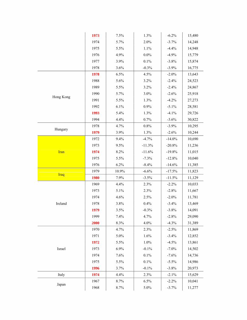
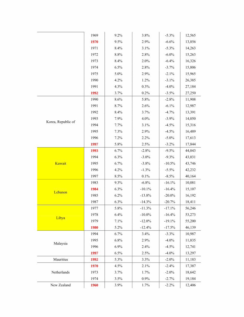
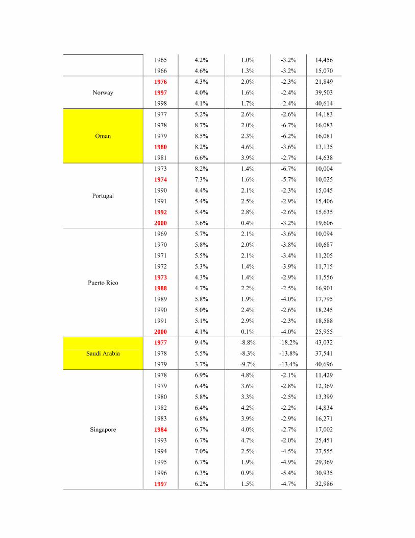
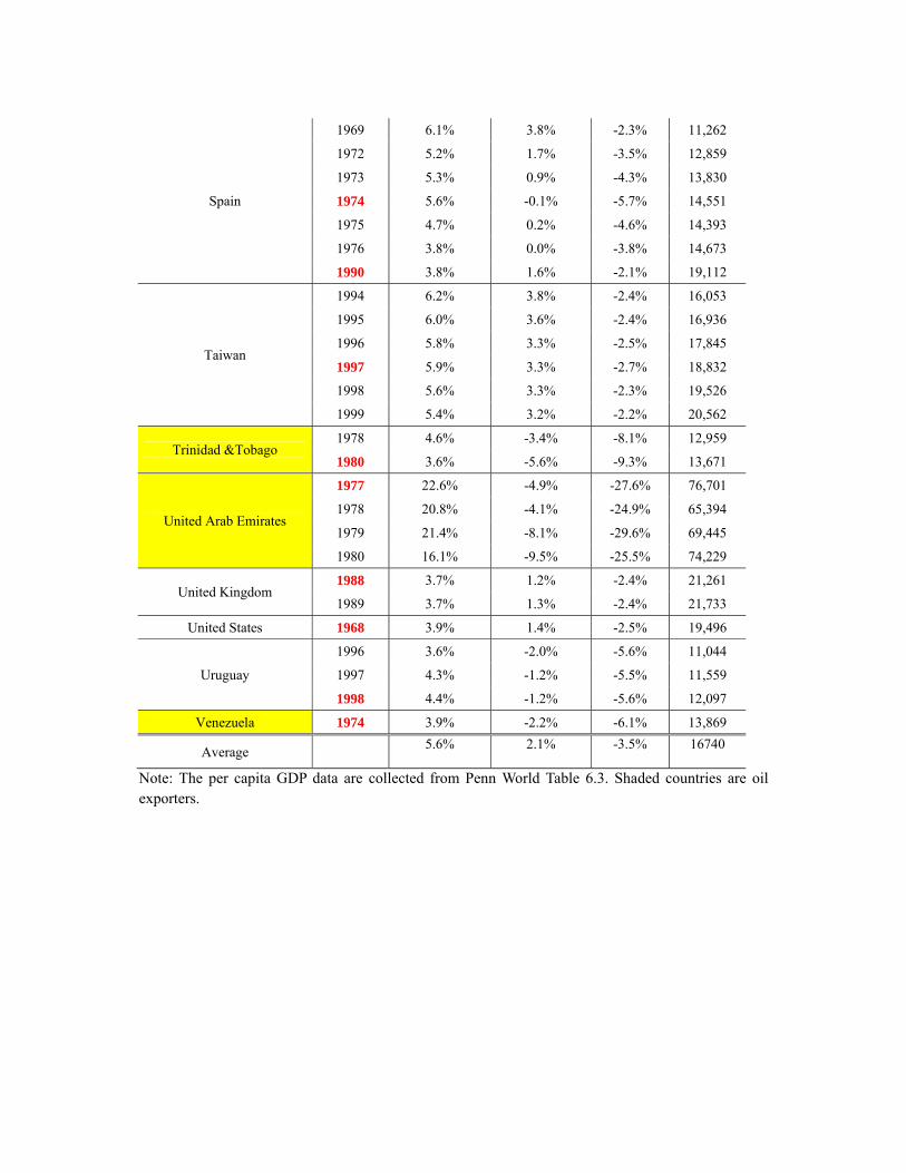
Table 1 lists all the slowdowns identified by this approach. In some cases the methodology identifies a string of consecutive years as growth slowdowns. For example, in Greece all years between 1969 and 1978 are identified as a slowdown. One way of dealing with this is to employ a Chow test for structural breaks to select only one year out of the consecutive years identified. For Greece we would then select 1973 as the year of growth slowdown because the Chow test is most significant for that year. In Table 1, the years chosen by the Chow test are denoted in red.

With this break point in hand, we next assign the value of 1 to the three years centered on the year of the growth slowdown, i.e. the dummy equals 1 for t t1, t and t 1 and zero otherwise.7 The comparison group consists of the countries that did not experience a growth slowdown in that same year. The sample includes all countries for which the relevant data are available including countries that have never experienced a growth slowdown. We drop all data pertaining to years t 2, … t 7 of the growth slowdown as a way of removing to remove the transition period to which either a 0 or 1 may not be clearly assigned.

In addition to focusing on the dates identified above, we also report the results when we do not employ the Chow test and leave the consecutive years as they are, i.e. the dummy indicating a slowdown is set equal to 1 for the entire run of consecutive years (and, in addition to the observations for that country one year before and after those selected years of the growth slowdown). In our regression analysis we report the results both for the sample of all countries covered by PWT when the manufacturing employment share is not used as an explanatory variable, as well as for a somewhat smaller sample when we employ the manufacturing share. Finally, since oil-exporting countries are very volatile behavior and exhibit growth slowdowns at per capita incomes very different from other countries (see below), we also report the results when oil countries are removed. (In Table 1, oil exporters are shaded in yellow.) Throughout, we report robust standard errors that take into considerations of the panel structure of the probit model.

3. What Slowdowns Look Like

At the bottom of Table 1 we report the average values for all non-oil-exporting countries. On average, high growth came to an end at a per capita GDP of $16,740, in 2005 constant international prices. (The median is $15,058.) At that point the growth rate slowed from 5.6 to 2.1 per cent per annum. For purposes of comparison, note that China’s per capita GDP, in constant 2005 international prices, was $8,511 as of 2007, India’s $3.826, Brazil’s $9,645. These are the latest compatible figures provided by Penn World Tables.

Around this average of $16,740 there is considerable variation. Figure 1 summarizes

the frequency distribution by per capita income in the form of a bar graph, oil exporters excluded.8 In some cases, explanations for these variations are well known, while in others

7 Again, this directly follows Hausmann, Pritchett and Rodrik. 8 On the exclusion of oil exporters see the discussion below. The reader’s eyes will no doubt be drawn to the

explaining them “will require further study.” At this point we limit ourselves to a few observations.

First, the list in Table 1 passes the smell test that most of the episodes are well known and plausible. The methodology locates slowdowns for a number of European countries in the first half of the 1970s, when the quarter-century-long “golden age” of rapid economic growth inaugurated by the Marshall Plan and postwar recovery is widely seen as coming to a close (Crafts and Toniolo 1976). It detects a slowdown in Argentina in 1998, just prior to that country’s financial difficulties coming to a head (as discussed by de la Torre, Levy-Yeyati and Schmukler 2002). The slowdown in Korea is centered in 1997, again on the eve of a financial crisis, although in this case we see a steady but significant deceleration over the course of preceding years (as described in Eichengreen, Perkins and Shin forthcoming).

A number of countries do not appear in this list, for good reason. Most of these, like China, continue to have per capita incomes below $10,000 in 2005 prices and are therefore excluded by construction – the idea being that the kind of slower growth with which we are concerned should not simply be a conjunctural phenomenon or a reflection of inability to develop but rather should be associated with increasing economic maturity.9 In practice, this condition does not appear to be especially restrictive. If we reduce the $10,000 threshold to $7,500, we do in fact pick up 15 additional cases, but most of these appear to be reflections of special circumstances that depressed growth relative to trend for an extended period rather than sustained slowdowns in increasingly mature economies. They include Portugal’s slowdown around the time of its mid-1970s revolution, Romania when President Ceausescu put the economy through the wringer in order to repay the debt, Mexico’s slowdown at the end of the 1970s and beginning of the 1980s when its foreign-borrowing binge came to an end, and the slowdown in Cuban growth over the course of the 1980s as Soviet aid was curtailed. For what it is worth, the mean income at which slowdowns occur falls from $16,740 to $15,092 when we reduce the minimum-income threshold from $10,000 to $7,500.10

Second, in the majority of the countries experiencing slowdowns, this event is centered at a single point in time and a particular level of per capita income. In a few exceptional cases, growth decelerates in steps. Japan is a well-known example: there is a first slowdown in the early 1970s (our methodology centers this on year 1970 itself, where the difference in the growth rate averages 6.6 per cent per annum between the seven preceding and subsequent years), and then a second slowdown in the 1990s (centered on 1992, where the deceleration is an additional 3.5 per cent). Obviously, these magnitudes are exceptional; there is no other country where slowdown episodes produce a cumulative deceleration of fully 10 percentage points (there being no other economy that both experienced such a dramatic economic miracle and then such a complete growth disaster). Qualitatively if not quantitatively, we see a similar pattern in Austria, which experienced a Wirtschaftswunder after World War II before decelerating first in 1961 and then again in 1974, and in Spain, where there is evidence of a two-step deceleration centered around 1974 and 1990.

Most other countries for which the methodology picks out more than one growth deceleration are cases where, after an extended period of slower growth, economic reforms

four high-income slowdowns in the figure. These are for Hong Kong, Singapore, Japan and Norway, all of which are discussed further in what follows. 9 Or at least adolescence. 10 The median falls from $15,058 to $13,859.

lead to a period of faster growth followed by a second deceleration: examples include Argentina, Hong Kong Ireland, Israel, Norway, Portugal, and Singapore. In Norway the story is oil and natural gas, which led first to a marked uptick in growth in the 1980s and 1990s, giving way subsequently to deceleration. Still, in the vast majority of cases it seems appropriate to speak of a specific point in time and a particular level of per capita income at which a country’s previously rapid rate of growth slowed down.

A final observation concerns outliers. Very small open economies like Hong Kong and Singapore appear to experience their growth decelerations at unusually high levels of per capita GDP. It is tempting to also place Israel in this camp. It will be interesting to explore whether they are different because they are so small or because they are so open.

Oil exporters also are unusual in that they are able to maintain high rates until higher per capita incomes are reached than is customary for other countries. A moment’s reflection suggests that this is obvious: large amounts of oil that can be extracted at low cost shift up the entire per capita income profile, other things equal. Note that this is not inconsistent with the well-known observation about the potential negative impact on growth of resource abundance (“the resource curse”), since we focus here on the change in growth rates around the time of the slowdown, and not on their earlier absolute rate. All that we require for inclusion in the sample is that per capita income was growing by at least 3.5 per cent per annum over period prior to the slowdown. But it clearly will be important to distinguish oil exporters and treat them differently from other countries in the analysis that follows.

4. Proximate Sources of Slowdowns

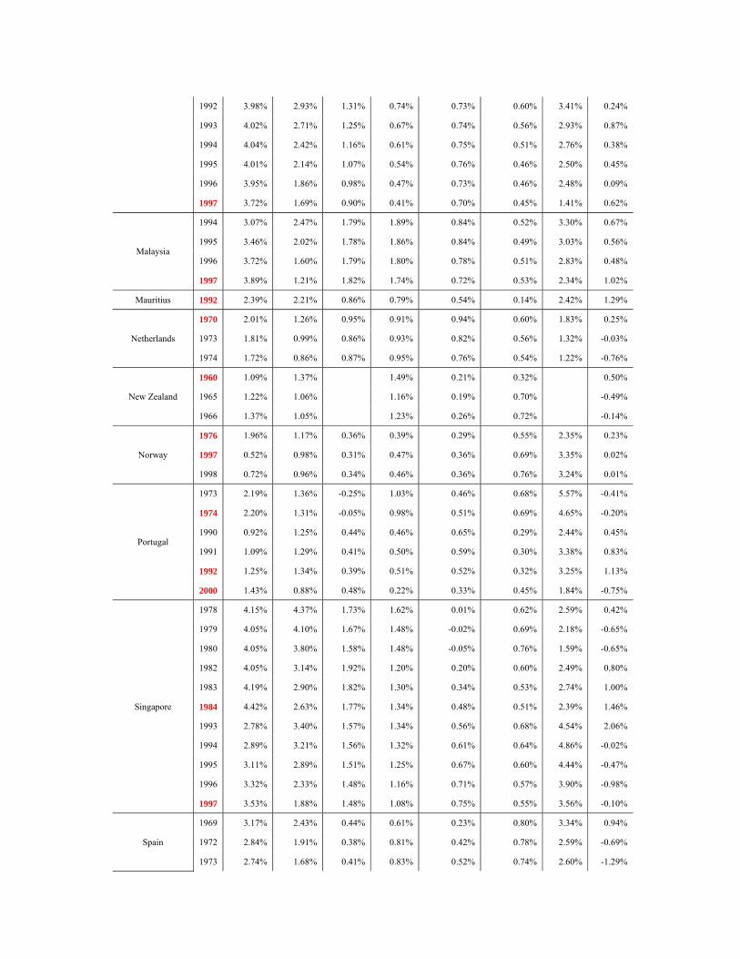
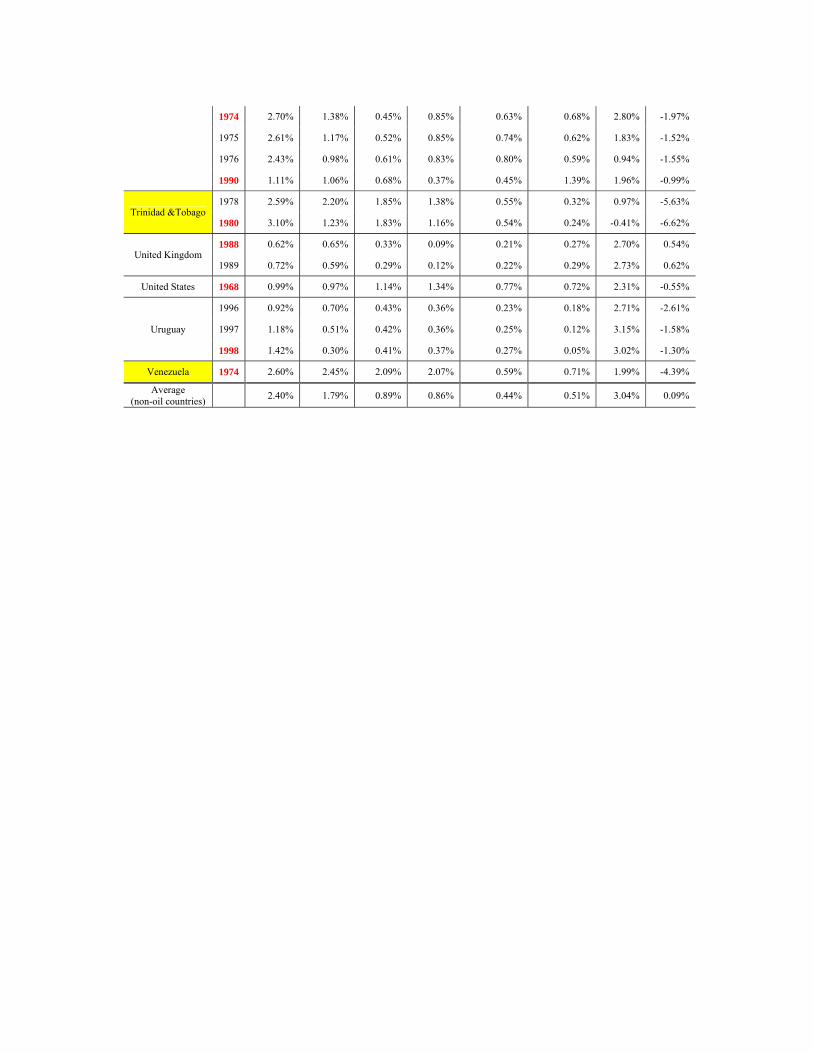
A first cut at the question of why slowdowns occur asks: which component of the standard growth-accounting framework – capital input, labor input, human capital input, or technical change – accounts for the bulk of the slowdown? To answer this question we use the standard growth-accounting framework, as implemented by inter alia Bernanke and Gurkaynak (2001), whose estimates of labor’s share of income we utilize here. We measure labor input as population between the ages of 15 and 64, from the World Bank’s World Development Indicators, while human capital data are from Barro and Lee (2010).

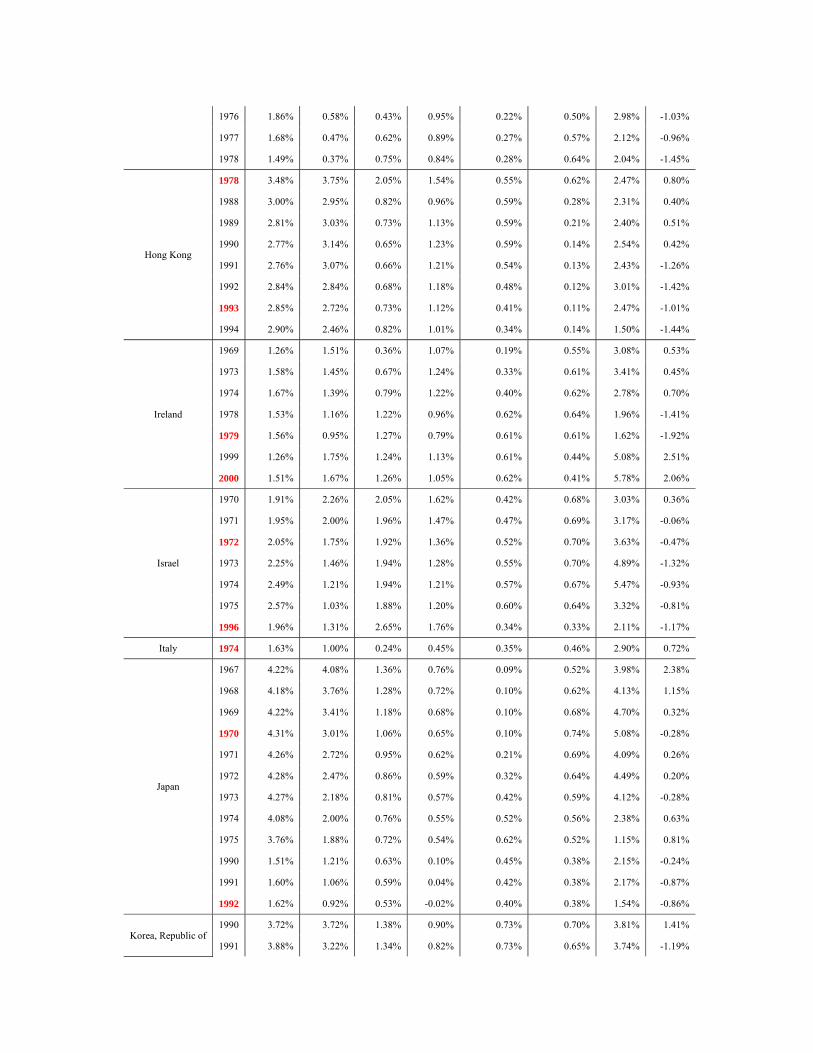
In Table 2 we report two sets of growth accounting results, the first of which uses labor share calculated a la Bernanke and Gurkaynak, whereas the second simply sets labor’s share equal to 0.65 for each country. In Table 2.1 we see that the contribution of the growth of the capital stock fell from 2.40 per cent to 1.79 per cent around the time of slowdowns. The contribution of labor growth fell more modestly, from 0.89 to just 0.86 per cent, while that of the growth of human capital actually increased (from 0.44 to 0.51 per cent). Much more dramatic is the decline in the contribution of TFP growth, from 3.04 to 0.09 per cent. Growth slowdowns, in a nutshell, are productivity growth slowdowns.11 85 per cent of the slowdown in the rate of growth of output is explained by the slowdown in the rate of TFP growth. The details in Table 2.2 are different but the story is the same.12

The intuition for this is straightforward. Slowdowns coincide with the point in the growth process where it is no longer possible to boost productivity by shifting additional

11 The smaller contribution of capital accumulation may not be negligible, but it is dwarfed by the decline in the contribution of TFP growth. 12 The analogous figures are 2.49 to 1.88 per cent for capital, 0.91 to 0.86 per cent for labor, 0.45 to 0.50 per cent for human capital, and 2.83 to 0.05 per cent for TFP.

workers from agriculture to industry and where the gains from importing foreign technology diminish. But the sharpness and extent of the fall in TFP growth from unusually high levels of 3-plus per cent to virtually zero is striking.

Next we consider the determinants of growth slowdowns using a probit model. Since the share of employment in manufacturing is likely to be important for the timing of growth slowdowns, initially we limit the sample to observations for which we have this information. We regress our binary indicator of slowdowns identified using the Chow-test methodology on per capita GDP, the ratio of per capita GDP to that in the lead country, the dependency ratio, and the manufacturing share of employment, all of which we enter as quadratics. In addition we include the crude fertility rate.

In Tables 3.1 and 3.2 we report summary statistics for these variables for the full sample countries, for countries experiencing growth slowdowns, and for China, a country of special interest in this context (for obvious reasons).

As shown in Tables 4.1 and 4.2, per capita GDP is consistently the most important variable: both per capita GDP and its squared are highly significant.13 If we use the regression result in column (1), the peak probability of slowdown occurs when the per capita GDP reaches $15,389 in 2005 prices, broadly in line with the simple statistics of Table 1. The ratio measure of per capita income also enters as expected; both the level and squared terms are significantly different from zero when entered alone; when entered together with per capita income, the latter dominates, although the ratio of per capita income to that in the lead country often approaches significance at conventional confidence levels. Column 2 suggests that a growth slowdown typically occurs when per capita income reaches 58 per cent of that in the lead country. The manufacturing employment share and the manufacturing employment share squared are also significant. The peak probability occurs when manufacturing accounts for 23 per cent of total employment. Interestingly, the dependency-ratio variables are not statistically significant, and the fertility rate, when significant, enters with a positive coefficient.

It is plausible that the likelihood of a growth slowdown increases as well with the speed of growth in the seven-year pre-slowdown period. Intuitively, the more aggressive the exceptional measures taken to boost the economy’s rate of growth, the less likely it is that its exceptionally rapid growth can be maintained. Consistent with this presumption, the pre-crisis growth rate enters positively and highly significantly in columns 4-6 Table 4.1; the other effects for their part remain unchanged. Adding this additional independent variable does, however, shift upward the level of per capita income at which the slowdown is predicted to occur, other things equal, to the $18,569-$18,973 range.

Tables 4.2 and 5-6 show that these patterns are robust to a variety of changes in sample and specification. Table 4.2 retains the entire string of years identified by the slowdown methodology (when these exist) rather than using a Chow test to pick out an individual year. Tables 5.1 and 5.2 use the Chow test and consecutive-year definitions but employ the entire sample of countries rather than just those for which manufacturing employment is available. Tables 6.1 and 6.2 do the same but remove oil exporters from the sample. There are a few differences worth noting. When we include the entire string of slowdown years (Table 4.2), a higher fertility rate is positively and significantly associated

13 Here, and for that matter in virtually any specification.

with the probability of a growth slowdown. In this variant, slowdowns begin at lower levels of per capita GDP ($12,802 in Table 2) and at a lower ratio of per capita income relative to the lead economy (0.54 rather than 0.58).

5. Extensions

Our preferred results are those in Tables 6.1 and 6.2, where the sample includes as many countries as possible other than oil exporters. We now use them as a basis for considering the impact, if any, of other country characteristics and policies.

For example, one might conjecture that authoritarian regimes are more or less prone to growth slowdowns than democracies, or that countries experiencing a shift in political regime in one direction or the other are more vulnerable to slowdowns.14 Financially open economies might be more prone to growth slowdowns insofar as they are exposed to capital flow reversals or less prone to slowdowns insofar as they can successfully finance investment externally. Trade openness might reduce the likelihood of experiencing a slowdown (or so cases like Hong Kong and Singapore suggest), while terms of trade shocks might increase that likelihood.15 Old-age and youth dependency rates might have different implications. At the same time, the fact that a number of these variables (the nature of the political regime or trade and financial openness) have been shown to be less than robustly related to economic growth suggests that they might also be less than robustly related to sharp (negative) changes in economic growth of the sort we analyze here.

It is this last presumption that appears to be borne out. Financial openness, terms of trade shocks, and political regime changes do not appear to have a significant impact on the likelihood of growth slowdowns.16

Higher old age dependency rates, in contrast, do appear to increase the likelihood of a slowdown, which is intuitive insofar as it is associated with lower savings rates and slow labor force participation rates (Table 6.2, column 6). Note that distinguishing the old age and youth dependency ratios, as here, also eliminates the anomaly of a positive coefficient on the fertility rate seen in some columns of Tables 4.1-4.2.

The estimates for trade openness, although not entirely consistent, do provide some support for the hypothesis, at least when openness is entered together with terms of trade shocks. In Table 6.2, both the linear and squared terms in openness are statistically significant at the one per cent confidence level. Economies more open to trade are less likely to experience slowdowns, other things equal, where the presence or absence of terms of trade

14 Again we following Hausmann, Pritchett, and Rodrik, political regime change is defined as one if during a five year period the regime change increases (“Poschange”) or reduces (“Negchange) the policy score. 15 Trade openness and its squared term. Trade openness is measured by “constant price openness” as defined in

the Penn World Tables: exports plus imports divided by GDP in constant prices. Financial openness index constructed by Chinn and Ito (2008), with updates kindly supplied by the authors. For terms of trade shocks. We followed Hausmann, Pritchett and Rodrik, defining a dummy variable denoted TOT, which takes a value 1 whenever the change in the terms of trade from year t to t −4 is in the lower 10 percent of the entire sample. This variable captures exceptionally adverse external circumstances. 16 Failure to find effects for financial openness could conceivable reflect the fact that the Chinn-Ito index starts

in 1970 for most countries (except Bahrain (1976), Hungary (1986), Mauritius (1972), Oman (1977) and United Arab Emirates (1976)). This forces us to drop earlier growth slowdowns like those of Australia (1968), Austria (1961), Demark (1964, 1965), Greece (1969), Ireland (1969), Japan (1967-1969), New Zealand (1960, 1965, 1966), Spain (1969), and the United States (1968).

shocks is importantly among the other things that must be held equal. This effect reaches a peak when exports and imports as a share of GDP approach 96 per cent. This result is consistent with Kehoe and Ruhl (2010) who argue that trade openness is more important during the early stage of growth and institutions become more important at the later stages.

This brings us back to the cases of Hong Kong and Singapore, small open economies that seem to have slowed down at much higher than average incomes. When we add a variety of measures of economic size – aggregate GDP or population, for example – they appear to have no effect on the likelihood of experiencing a slowdown. If these economies are unusual, it would appear that this is because they are so open, not because they are so small. Note, however, that the sum of exports and imports is considerably above 96 per cent in both economies, which suggests that other factors (economic policies and proximity to China are plausible candidates) also account for their exceptional behavior.

One might also ask whether slowdowns are more likely in high-investment, high-consumption, or high-government-spending economies. We therefore examine the impact of the ratios of these variables to GDP, where the ratio in question is entered in both level and squared form.17 Only the consumption share and its square are consistently significant. The consumption ratio enters negatively: as consumption rises from low levels, the probability of a slowdown falls. The probability of slowdown is minimized when consumption is 62 or 64 per cent of GDP (Table 6.1 or 6.2, respectively). In addition, there is some evidence that the investment ratio matters for the probability of growth slowdowns: slowdowns are less likely in countries that maintain exceptionally high investment rates, other things equal (the quadratic of the investment rate is negative and significant in Table 6.2, column 13).

6. Effects of Economic Policy

How is the probability of experiencing a growth slowdown affected by economic policy? We take a first cut at answering this question by adding to our basic model, which takes per capita income, per capita income squared and the pre-slowdown rate of growth as key regressors, the average rate of inflation from t-7 to t-1, the variability of that inflation rate (calculated as the standard deviation of past inflation over the same period), and the variability of the exchange rate (calculated as the standard deviation of the nominal exchange rate over the same period).

In addition, we include the undervaluation of the real exchange rate over the same seven years. The real exchange rate is defined as the nominal exchange rate (e) relative to purchasing power parity (PPP): RER = e/PPP. We compute the “normal” or “equilibrium” real exchange rate for a large sample of countries, regressing the real exchange rate on per capita GDP, demographic controls, and a vector of time dummies. The extent of real over- or undervaluation is then the difference between the actual real exchange rate and the fitted value.18

Results are in Tables 7.1 and 7.2. The most consistently significant policy variable is the degree of real undervaluation.19 Strikingly, this enters positively: countries with more dramatically undervalued currencies are more likely to experience growth slowdowns, other

17 Note that we continue to control for per capita income and other characteristics. 18 Nothing changes when we exclude the measures of demographic structure from the first part of this exercise. 19 In addition, there is some indication that a more variable exchange rate heightens the risk of a slowdown (exchange rate variability is statistically significant in one of the two tables).

things equal. This is more than simply the tendency for real undervaluation to translate into faster output growth, since we are controlling separately for the pre-slowdown growth rate. It may be that countries that rely on undervalued exchange rates to boost economic growth are more vulnerable to external shocks resulting in sustained slowdowns. It may be that real undervaluation works as a mechanism for boosting growth during the early stages of development when a country relies on shifting labor from agriculture to export-oriented manufacturing but not in subsequent stages when growth becomes more innovation intensive, but governments are reluctant to abandon the earlier policy strategy, leaving the economy increasingly susceptible to slowing down. It could be that real undervaluation allows imbalances and excesses in export-oriented manufacturing build up, as in Korea in the 1990s, through that channel making a sustained deterioration in subsequent growth performance more likely.

An alternative approach to analyzing the impact of economic policies is by estimating a hazard model. The dependent variable in the typical hazard model is the duration of time until an event occurs. In our model, however, the dependent variable is per capita GDP. The idea is that since the probability of growth slowdown increases with per capita GDP, we can treat per capita GDP in the same way as duration of time in the typical model. In this setup, the estimated coefficients indicate the impact of the regressors on the hazard rate of slowdown at the corresponding per capita GDP level. We removed countries that never have experienced slowdown and those with per capita GDPs above $20,000.20 For countries that never experience a growth slowdown, but with per capita GDPs below $20,000, we use their per capita GDP in year 2000, this being the last year we can calculate the 7-year post-slowdown growth rate. Table 8.1 considers only the first slowdown for each country, while Table 8.2 allows for multiple slowdowns. In the latter case we allow for clustering effects when estimating the standard errors. In estimating the model, we also removed oil countries.

The results suggest that again suggest that countries with undervalued real exchange rates are more vulnerable to slowdowns. In addition there is now some indication in this specification that policy instability – high and variable inflation rates – are precursors to slowdowns. In the consolidated specification in the last column of Table 8.1, both the level and variability of inflation enter with significant negative coefficients, suggesting that in these countries slowdowns come at lower per capita incomes. The results in Table 8.2 reinforce the finding.

7. Implications for China

While an eventual growth slowdown is common to all fast-growing economies, special anxiety attaches to the question of how and when Chinese growth might slow. China in recent years has accounted for a substantial fraction of global growth. A sharp slowdown in Chinese growth in the not-too-distant future could therefore have important implications for global expansion. In China itself, there could be implications for social stability. On both counts the ramifications could be far reaching.

A few earlier studies have contemplated this question. Lee and Hong use a growth accounting framework, distinguishing capital, labor, and human capital, and estimate equations for TFP growth, the growth of the capital/labor ratio, and the savings rate for a

20 The reason for removing these countries is that the U.S. experienced growth slowdown when its per capita

GDP is $19,496, and it is unlikely that a country never experiences a slowdown until that level.

panel of countries. These variables depend on their own past levels.21 Other exogenous drivers include years of schooling and the growth of the stock of patents in the case of TFP growth, demographic variables, openness, and the strength of property rights in the case of the growth of the capital/labor ratio, and demography variables in the case of the savings rate. China being an outlier with its especially rapidly growing capital/labor ratio, a dummy variable for the PRC is included in some variants of that equation, generating alternative forecasts for the countries future growth performance.

Inserting plausible projections for the exogenous drivers, the authors project China as growing by 6.1 to 7.0 per cent per annum in the 2011-2020 decade and 5.0 to 6.2 per cent in the 2021-30 decade. This suggests that China will experience a slowdown, as defined by our criteria in this paper, sometime in the next ten years.22 From an accounting perspective, this reflects slower growth of all four proximate determinants of the aggregate rate of growth: slower labor force growth, a slower increase in educational attainment, a slower rate of increase in the capital stock and, most importantly, a slowdown in the country’s heretofore rapid rate of TFP growth. From an economic standpoint, slower growth results from the convergence of TFP and the capital/labor ratio to advanced-country values, slower growth of educational attainment once school enrolment rates have reached reasonably high levels, and ageing of the population.

These findings are broadly in line with the conclusions of other similar studies. Taking the mid-points of Lee and Hong’s estimates yields a forecast of 6.1 per cent per anum over the 2011-2030 period. Wilson and Stupnytska (2007)), in a study adopting a simplified version of the same methodology, produced an estimate of 5.8 per cent for 2008-2030. Maddison (2007) is more pessimistic, forecasting China’s annual average growth as slowing to 5.0 per cent between 2004 and 2030.23 Buiter and Rahbari (2011), relying heavily on the historical relationship between growth and convergence, project growth of per capital income of 5.0 per cent between 2010 and 2050 and, by implication, very slightly faster growth of overall GDP.

Basing his projections largely on the evolution of demographic trends and with optimistic assumptions about the returns to further investment in education, Fogel (2007) projects Chinese growth as running at 8.4 over the longer period 2001-40. While the other papers all imply that a significant growth slowdown is coming, the implications of Fogel’s study, in this respect, are less clear. Given actual performance in the most recent decade, his figures imply downshift to 7.9 per cent per annum growth in the course of the next three decades. If this downshift occurs abruptly, it would just barely constitute a slowdown according to our criteria, but spread over three decades it would not. Conference Board (2010) offers a base scenario in which growth proceeds by 9.2 per cent per annum in 2010-2015 and 7.9 per cent per annum in 2015-2020, by our metric avoiding a slowdown. But it also offers a pessimistic scenario in which the economy’s growth slows from first to 6.1 per cent per annum and then to 3.9 per cent per annum between the first and second halves of the current decade.

21 Thus, the rate of TFP growth is negatively related to its initial level, just as the growth of the capital/labor ratio is negatively related to its past level. 22 The differences within each period reflect different assumptions about the evolution of investment in education, the growth of the stock of patents and the strength of property rights. 23 Maddison’s forecasts are purely judgmental; they are not grounded in an explicit model.

Our results can be used to address the question of whether an abrupt slowdown is likely and if so when. Both China’s openness and high investment rate point away from the likelihood of a slowdown. Other considerations, however, suggest that a slowdown may be coming sooner rather than later. Recall that they suggest that the probability of a slowdown is highest when per capita GDP reaches $16,740 U.S. (year 2005 international) dollars, when the ratio of per capita income to that in the lead country is 58 per cent, and when the share of employment in manufacturing reaches 23 per cent. In Table 3.2 we see that China’s per capita GDP is $8,511 U.S dollars and the ratio of China’s per capita GDP to that in the U.S. is 19.8 per cent in 2007. If China grows at 9.3 per cent, which is the average growth rate of per capita GDP for the most recent ten years in the Penn World Table (1998-2007), by 2015 China’s per capita GDP reaches $17,335, just exceeding our slowdown threshold. If China grows more modestly at 7 per cent, then per capita GDP reaches the threshold level in 2017.

If the probability of slowing down is thought to depend on the country’s GDP per capita relative to that in the lead country (the United States), forecasts for U.S. growth also matter. If the U.S. grows at 1.9 per cent per annum, the average growth rate of per capita GDP in 1998-2007, then the ratio of Chinese to U.S. GDP per capita will still be only 35 per cent in 2015 even if China grows at 9.3 percent. But if the current financial crisis substantially slows U.S. growth rate to 1 per cent through 2015, then the ratio increases to 37 per cent. Either way, this remains well below the 58 per cent ratio which, historically, has been the point where fast-growing catch-up economies slow down. If we assume 9.3 per cent Chinese growth and 1.9 (1.0) U.S. growth, then China reaches 58 per cent of U.S. per capita income in 2023 (2021).

China’s share of manufacturing in total employment was 11.3 per cent in 2002, the latest year for which data are available.24 In the absence of further figures we assume that this fraction has been growing at one per cent per annum. If this is right, it suggests that the share of employment in manufacturing is now within hailing distance of the 23 per cent where historical comparisons suggest that growth slows down.

Our results further suggest that the fact that Chinese growth has been unusually fast, that its growth has been associated with what is widely viewed as a chronically undervalued exchange rate, that the old-age dependency ratio is rising, and that the consumption share of GDP is exceptionally low heightens the likelihood of an imminent slowdown. Raising the growth rate from 5 to 10 per cent, the difference between the emerging market average and China, raises the probability of a slowdown by 38 to 71 per cent (depending on whether we use estimates based on Chow-test break points or the consecutive slowdown points). Assuming that the renminbi is undervalued by 46 per cent (the estimate we obtain from the real exchange rate regression in this paper) raises the probability of a slowdown by 22 to 71 per cent. That the consumption share of GDP is 48 rather than 64 per cent (the latter, recall, being the ratio that minimizes the likelihood of slowing down) raises the probability of a slowdown by 16 to 73 per cent. The fact that China’s old-age dependency ratio is 10.1 rather than 9.4 per cent raises the probability of a slowdown by 3.5 to 77 per cent. Finally, the fact that China’s inflation rate has been rising heighten the likelihood of a slowdown, other things equal.

24 We obtained this figure from National Bureau of Statistics of China. The most recent data for the

manufacturing employment share is for 2002. After that the National Bureau reports the employment share for “secondary industry,” a category that includes other sectors in addition to manufacturing industries.

We can use a selection of our estimated equations together with 2007 values of the independent variables to estimate the likelihood of a Chinese slowdown. Using the coefficients in Table 6.2, columns 6 and 13, where the key independent variables are per capita income, the pre-slowdown rate of growth, demographic structure (in column 6) and trade openness and the composition of spending (in column 13) puts the probability at 77 and 73 per cent. Table 72, column 5, where the independent variables are policy measures (inflation, inflation variability and real undervaluation), this procedure puts the probability of a slowdown at 71 per cent. These are certainly non-negligible odds.

One should of course exercise special caution when extrapolating to China from the experience of other countries. Never before has such a large country grown so fast for such an extended period. China’s huge size and geographical diversity differentiate it from earlier fast growers such as Japan, Korea and Taiwan. Coastal regions such as the Pearl River Delta and Zhejiang have substantially outperformed central and western regions up to now. The latter therefore remain further below the per capita income threshold for slowdowns. If the growth miracle is transplantable within China, then the economic development of the interior provinces, which have larger populations than most countries and are home to a substantial fraction of China’s own population, can continue to sustain the country’s growth for years to come. The government is already extending physical infrastructure, such as highways and railways, to less developed provinces to prepare them for this transition.

There are China-specific downside risks to consider as well. These include the possibility of financial instability. They include social instability arising from large and growing inequality. To be sure, neither financial nor social instability is unique to China. Nor is their association with growth slowdowns: South Korea, for example, experienced social instability in the late 1980s and financial instability in the late 1990s, the years bracketing that county’s growth slowdown. Still, the broader point of the importance of taking into account China’s own unique structural characteristics when assessing the country’s growth prospects continues to apply.

How do our results relate to the debate over rebalancing the Chinese economy? The empirical association between low levels of consumption and an undervalued exchange rate on the one hand and a relatively high probability of a slowdown on the other reinforces a point made by foreign commentators and Chinese officials alike that the process of rebalancing the economy away from exports and allowing the renminbi exchange rate to appreciate from its historically low levels is best initiated sooner, while Chinese growth is strong and other preconditions for its maintenance are still in place, than later, when those shifts are more likely to be sharply discontinuous and disrupt the growth process. For example, one suspects that an economy that is unusually dependent on investment and net exports (and insufficiently dependent on domestic consumption) may be vulnerable to a sudden drop in the marginal efficiency of investment or a disruption to its foreign market access, either of which could be severely disruptive to the old growth model. Better, it follows, to start the process of eliminating those imbalances and limiting the danger of such disruptions while the going is good.25

25 The fact that it may take considerable time to raise the consumption share of GDP to the middle-income-country norm, for the simple reason that it may take time to build a social safety net, develop financial markets, and undertake the other reforms necessary to limit precautionary saving, works in the same direction.

8. Conclusion

We have recently grown accustomed to a world of exceptionally rapid catch-up growth in late-developing countries. China and other emerging markets have come to account for the majority of the growth of global demand, and the consensus is that they will continue to do so going forward.26 Economies as geographically and economically diverse as Germany and South Korea have come to depend on rapidly-growing catch-up economies for incremental demand for their exports. That incomes in these countries will continue to rise and that the marginal propensity to spend on foodstuffs is higher at low and middle incomes is reason to think that higher food prices are here to stay. That emerging markets like China are energy intensive economies suggests that current upward pressure on commodity prices is more than a passing phase.

This perspective is based on extrapolating the experience of the current cohort of high-growth economies. But there is also another, very different way of extrapolating historical experience: looking at earlier rapidly-growing catch-up economies suggests that all fast growing economies eventually slow down. The question is when. And the most immediate incarnation of the question is “when China?”

As with all things economic, forecasting growth slowdowns is an imperfect science. International experience suggests that rapid-growing catch-up economies slow down significantly, in the sense that the growth rate downshifts by at least 2 percentage points, when their per capita incomes reach around $17,000 US in year-2005 constant international prices, a level that China should achieve on or soon after 2015. Our estimates suggest that high growth slows down when the share of employment in manufacturing is 23 per cent; while current data on employment shares in China are not readily available, observation and extrapolation suggest that China is nearly there. Our estimates similarly suggest that growth slows when income per capita in the late-developing country reaches 57 per cent of that in the country that defines the technological frontier, a level that China is likely to reach only somewhat later.

Of course, there is no iron law of slowdowns. There is unlikely to be a mechanical relationship between per capita incomes and growth slowdowns. How long rapid growth is successfully maintained depends also on economic policy. Economies that are more open to trade seem to be able to maintain high growth rates for longer; this will reassure those who hope that China will be able to continue driving global growth. But higher old-age dependency ratios make growth slowdowns more likely, and China will have a higher old-age dependency ratio in the not-too-distant future. Higher and more volatile inflation rates also make slowdowns more likely, and there are reasons to worry about China on this score.

Most provocatively, slowdowns are more likely and occur at lower per capita incomes in countries that maintain undervalued exchange rates and have low consumption shares of GDP. The nature of this association remains, at this point, a matter of speculation. It could be that countries that rely on undervalued exchange rates are more vulnerable to external shocks. It may be that real undervaluation that works well as a mechanism for boosting growth in the

26 By some estimates, China alone is accounting for 30 per cent of global demand growth, the BRICs collectively 45 per cent, and emerging markets and developing countries as a whole a healthy majority of the total. Looking forward, Conference Board (2010) suggests in its base case scenario that emerging markets will account for 3.4 per cent of the global economy’s 4.4 per cent annual rate of economic growth over the coming decade.

early stages of development works less well later, when growth becomes more innovation intensive. It may be that real undervaluation allows imbalances and excesses in export-oriented manufacturing build up.

More generally, our results suggest that an exceptionally low consumption share of GDP is positively associated with the probability of a slowdown. This is more than simply the same real-undervaluation result in another guise. While an undervalued exchange rate may be a driver of China’s imbalances, it is by no means the only one. In fact a wide range of factor price distortions favors the production of tradables over nontradables and thereby results in an unusually low consumption share of GDP. Lax corporate governance of state-owned enterprises limits pressure to pay out dividends and acts as a de facto subsidy for investment. The absence of a social safety net and well-developed domestic financial markets provide a strong incentive for precautionary saving on the part of households. This suggests additional margins on which Chinese policy can operate to limit the risk of a sharp growth slowdown.

In some circles, the assumption is pervasive that China will continue to grow rapidly. Equivalently, it is assumed that China will be able to avoid the middle income trap and jump to upper-middle-income-country status. But it is worth recalling that only a small group of countries successfully completed this transition in the second half of the 20th century, while a much larger group, in Latin America for example, are still struggling to escape the middle-income trap. Given China’s huge size and daunting array of structural challenges, completing this transition is far from a fait accompli.

Data Appendix

1. Growth Slowdown

Per capita GDP: Real GDP per capita (US$ in 2005 Constant Prices: Chain series)

Source: Penn World Tables 6.3

2. Growth Accounting

(1) Aggregate GDP

Per Capita GDP Population

Source: Penn World Tables 6.3

(2) Labor Force

Working Age Population between 15-64

Source: World Development Indicators 2010

For Taiwan, we use actual labor force from National Statistics of Taiwan.

(3) Capital

Authors’ calculations based on investment data

(4) Labor Share

Source: Bernanke & Gurkaynak(2001)

(5) Human Capital

Educational Attainment for Population aged 25 and over

Source: Barro and Lee (2010) Educational Attainment Dataset

3. Probit Regression

(1) Demography

Age Dependency Ratio, young: Percentage ratio of younger dependents (younger than 15) to the working-age population (15-64).

Source: World Development Indicators 2010

Age Dependency Ratio, old: Percentage ratio of older dependents (older than 64) to the working-age population.

Source: World Development Indicators 2010

Age Dependency Ratio: The percentage ratio of dependents (people younger than 15 or older than 64) to the working age population.

Source: World Development Indicators 2010

Fertility Rate: Birth per woman

Source: World Development Indicators 2010

(2) Manufacturing employment share

Source: EUKLEMS

(3) External sector

Terms of Trade: Net barter terms of trade index calculated as the percentage ratio of the export unit value index to the import unit value index, measured relative to the base year 2000

Source: World Development Indicators 2010.

The data before 1980 were obtained from Hiro Ito.

Trade openness in constant prices: The total trade (exports and imports) as a percentage of GDP

Source: Penn World Tables 6.3

Financial Openness: The index takes on higher values the more open the country is to cross-border capital transactions.

Source: Chinn-Ito Index

(4) Political regimes

Polity Index: The polity score captures the regime authority spectrum on a scale ranging from -10 (hereditary monarchy) to -10 (consolidated democracy).

Source: The Center for Systemic Peace)

Democracy Variable (Political rights): Political Rights are measured on a one-to-seven scale, with one representing the highest degree of Freedom and seven the lowest. Source: Freedom House

(5) Policy Variables

Inflation: CPI change over corresponding period of previous year

Source : IFS line 64XZF

Exchange Rate: US=1

Source: Penn World Tables 6.3

Real Exchange Rate: Exchange Rate divided by PPP

Source: Penn World Tables 6.3

Debt-to-GDP ratio: Total government debt as a percentage of GDP

Source: Reinhart-Rogoff (2010) data set

References

Asian Development Bank (2010), “The Future of Growth in Asia,” Asian Economic Outlook (October), pp.37-89.

Barro, Robert and Jong-Wha Lee (2010), “A New Data Set of Educational Attainment in the World, 1950–2010,” NBER Working Paper No. 15902 (April).

Ben-David, David and David Papell (1998), “Slowdowns and Meltdowns: Postwar Growth Evidence from 74 Countries,” Review of Economics and Statistics 80, pp.561-571.

Bernanke, Ben S. and Refet S. Gurkaynak (2001), "Is Growth Exogenous? Taking Mankiw, Romer and Weil Seriously," NBER Macroeconomics Annual 16, pp.11-57.

Brandt, Loren, Johannes Van Biesebroeck and Yifan Zhang (2011), “Creative Accounting or Creative Destruction? Firm-level Productivity Growth in Chinese Manufacturing,” Journal of Development Economics, forthcoming.

Buiter, Willem and Ebrahim Renbari (2011), “Global Growth Generators: Moving Beyond Emerging Markets and BRICs,” Citigroup Global Markets (21 February).

Chinn, Menzie and Hiro Ito (2008), “A New Measure of Financial Openness,” Journal of Comparative Policy Analysis 10, pp.309-322.

Conference Board (2010), Global Economic Outlook -2011, New York: Conference Board.

Crafts, Nicholas and Gianni Toniolo, eds. (1996), Economic Growth in Europe since 1945, Cambridge: Cambridge University Press.

De la Torre, Augusto, Eduardo Levy-Yeyati and Sergio Schmukler (2002), “Argentina’a Financial Crisis: Floating Money, Sinking Banking,” unpublished manuscript, World Bank (June).

Eichengreen, Barry, Dwight Perkins and Kwanho Shin (forthcoming), From Miracle to Maturity: The Growth of the Korean Economy, Cambridge, Mass.: Harvard East Asia Center.

Fogel, Robert (2007), “Capitalism and Democracy in 2040: Forecasts and Speculations,” NBER Working Paper no.13184 (June).

Gerschenkron, Alexander (1964), Economic Backwardness in Historical Perspective, Cambridge: Harvard University Press.

Hausmann, Ricardo, Lant Pritchett and Dani Rodrik (2004), “Growth Accelerations,” Journal of Economic Growth 10, pp.303-329.

Hausmann, Ricardo, Francisco Rodriguez and Rodrigo Wagner (2008), “Growth Collapses,” in Carmen Reinhart, Carlos Vegh and Andres Velasco (eds), Money, Crises and Transition, Cambridge, Mass.: MIT Press, pp.376-428.

Kehoe, Timothy and Kim Ruhl (2010), “How Have Economic Reforms in Mexico not Generated Growth?” NBER Working Paper no. 16580.

Lee, Jong-Wha and Kiseok Hong (2010), “Economic Growth in Asia: Determinants and Prospects,” unpublished manuscript, Asian Development Bank and Ewha Women’s

University (September).

Maddison, Angus (2009), Chinese Economic Performance in the Long Run, second edition revised and updated, 960-2030 AD, Paris: OECD.

Pritchett, Lant (2000), “Understanding Patterns of Economic Growth: Searching for Hills among Plateaus, Mountains and Plains,” World Bank Economic Review 14, pp.221-250.

Reddy, Sanjay and Camelia Miniou (2006), “Real Income Stagnation of Countries, 1960-2001,” unpublished manuscript, Columbia University.

Reinhart, Carmen and Kenneth Rogoff (2010), “From Financial Crash to Debt Crisis,” NBER Working Paper 15795 (March).

Rodrik, Dani (1999), “Where Did All the Growth Go? External Shocks, Social Conflict and Growth Collapses,” Journal of Economic Growth 4, pp.385-412.

Ros, Jaime (2005), “Divergence and Growth Collapses: Theory and Empirical Evidence,” in Jose-Antonio Ocampo (ed), Beyond Reforms: Structural Dynamics and Macroeconomic Vulnerability, Stanford: Stanford University Press, pp.211-232.

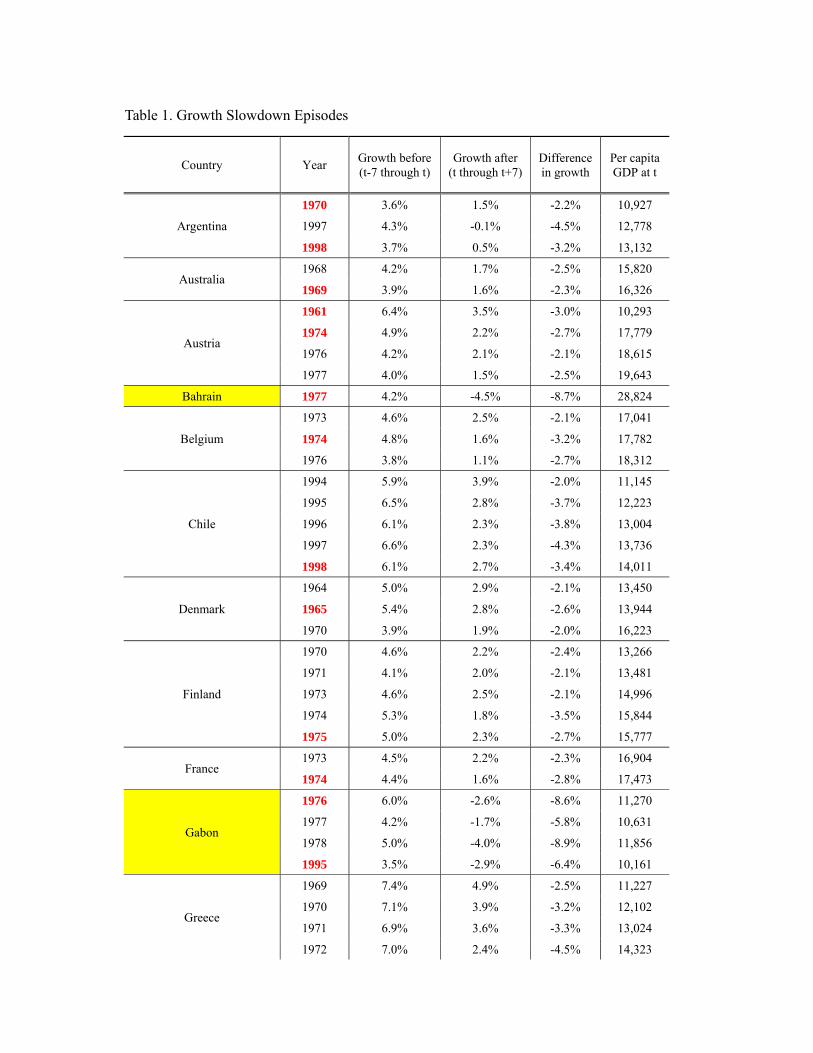
Table 1. Growth Slowdown Episodes

Country Year Growth before(t-7 through t)

Growth after (t through t+7)

Difference in growth

Per capita GDP at t

Argentina

1970 3.6% 1.5% -2.2% 10,927

1997 4.3% -0.1% -4.5% 12,778

1998 3.7% 0.5% -3.2% 13,132

Australia 1968 4.2% 1.7% -2.5% 15,820

1969 3.9% 1.6% -2.3% 16,326

Austria

1961 6.4% 3.5% -3.0% 10,293

1974 4.9% 2.2% -2.7% 17,779

1976 4.2% 2.1% -2.1% 18,615

1977 4.0% 1.5% -2.5% 19,643

Bahrain 1977 4.2% -4.5% -8.7% 28,824

Belgium

1973 4.6% 2.5% -2.1% 17,041

1974 4.8% 1.6% -3.2% 17,782

1976 3.8% 1.1% -2.7% 18,312

Chile

1994 5.9% 3.9% -2.0% 11,145

1995 6.5% 2.8% -3.7% 12,223

1996 6.1% 2.3% -3.8% 13,004

1997 6.6% 2.3% -4.3% 13,736

1998 6.1% 2.7% -3.4% 14,011

Denmark

1964 5.0% 2.9% -2.1% 13,450

1965 5.4% 2.8% -2.6% 13,944

1970 3.9% 1.9% -2.0% 16,223

Finland

1970 4.6% 2.2% -2.4% 13,266

1971 4.1% 2.0% -2.1% 13,481

1973 4.6% 2.5% -2.1% 14,996

1974 5.3% 1.8% -3.5% 15,844

1975 5.0% 2.3% -2.7% 15,777

France 1973 4.5% 2.2% -2.3% 16,904

1974 4.4% 1.6% -2.8% 17,473

Gabon

1976 6.0% -2.6% -8.6% 11,270

1977 4.2% -1.7% -5.8% 10,631

1978 5.0% -4.0% -8.9% 11,856

1995 3.5% -2.9% -6.4% 10,161

Greece

1969 7.4% 4.9% -2.5% 11,227

1970 7.1% 3.9% -3.2% 12,102

1971 6.9% 3.6% -3.3% 13,024

1972 7.0% 2.4% -4.5% 14,323

1973 7.5% 1.3% -6.2% 15,480

1974 5.7% 2.0% -3.7% 14,248

1975 5.5% 1.1% -4.4% 14,948

1976 4.9% 0.0% -4.9% 15,779

1977 3.9% 0.1% -3.8% 15,874

1978 3.6% -0.3% -3.9% 16,775

Hong Kong

1978 6.5% 4.5% -2.0% 13,643

1988 5.6% 3.2% -2.4% 24,523

1989 5.5% 3.2% -2.4% 24,867

1990 5.7% 3.0% -2.6% 25,918

1991 5.5% 1.3% -4.2% 27,273

1992 6.1% 0.9% -5.1% 28,581

1993 5.4% 1.3% -4.1% 29,726

1994 4.4% 0.7% -3.6% 30,822

Hungary 1978 4.7% 0.8% -3.9% 10,295

1979 3.9% 1.3% -2.6% 10,244

Iran

1972 9.4% -4.7% -14.0% 10,690

1973 9.5% -11.3% -20.8% 11,236

1974 8.2% -11.6% -19.8% 11,015

1975 5.5% -7.3% -12.8% 10,040

1976 6.2% -8.4% -14.6% 11,385

Iraq 1979 10.9% -6.6% -17.5% 11,823

1980 7.9% -3.5% -11.5% 11,129

Ireland

1969 4.4% 2.3% -2.2% 10,033

1973 5.1% 2.3% -2.8% 11,667

1974 4.6% 2.5% -2.0% 11,781

1978 3.8% 0.4% -3.4% 13,469

1979 3.5% -0.3% -3.8% 14,091

1999 7.4% 4.7% -2.8% 29,090

2000 8.3% 4.0% -4.3% 31,389

Israel

1970 4.7% 2.3% -2.5% 11,869

1971 5.0% 1.6% -3.4% 12,852

1972 5.5% 1.0% -4.5% 13,861

1973 6.9% -0.1% -7.0% 14,502

1974 7.6% 0.1% -7.6% 14,736

1975 5.5% 0.1% -5.5% 14,986

1996 3.7% -0.1% -3.8% 20,973

Italy 1974 4.4% 2.3% -2.1% 15,629

Japan 1967 8.7% 6.5% -2.2% 10,041

1968 8.7% 5.0% -3.7% 11,277

1969 9.2% 3.8% -5.3% 12,565

1970 9.5% 2.9% -6.6% 13,856

1971 8.4% 3.1% -5.3% 14,263

1972 8.8% 2.8% -6.0% 15,263

1973 8.4% 2.0% -6.4% 16,326

1974 6.5% 2.8% -3.7% 15,806

1975 5.0% 2.9% -2.1% 15,965

1990 4.2% 1.2% -3.1% 26,385

1991 4.3% 0.3% -4.0% 27,184

1992 3.7% 0.2% -3.5% 27,250

Korea, Republic of

1990 8.6% 5.8% -2.8% 11,908

1991 8.7% 2.6% -6.1% 12,987

1992 8.4% 3.7% -4.7% 13,391

1993 7.9% 4.0% -3.9% 14,050

1994 7.7% 3.1% -4.5% 15,316

1995 7.3% 2.9% -4.5% 16,489

1996 7.2% 2.2% -5.0% 17,613

1997 5.8% 2.5% -3.2% 17,844

Kuwait

1993 6.7% -2.8% -9.5% 44,043

1994 6.3% -3.0% -9.3% 43,031

1995 6.7% -3.8% -10.5% 43,746

1996 4.2% -1.3% -5.5% 42,232

1997 8.5% 0.1% -8.5% 40,164

Lebanon

1983 9.3% -6.8% -16.1% 10,081

1984 6.3% -10.1% -16.4% 15,107

1985 6.2% -13.8% -20.0% 16,192

1987 6.3% -14.3% -20.7% 18,411

Libya

1977 5.8% -11.3% -17.1% 56,246

1978 6.4% -10.0% -16.4% 53,273

1979 7.1% -12.0% -19.1% 55,200

1980 5.2% -12.4% -17.5% 46,139

Malaysia

1994 6.7% 3.4% -3.3% 10,987

1995 6.8% 2.9% -4.0% 11,835

1996 6.9% 2.4% -4.5% 12,741

1997 6.5% 2.5% -4.0% 13,297

Mauritius 1992 5.3% 3.3% -2.0% 11,183

Netherlands

1970 4.5% 2.1% -2.4% 17,387

1973 3.7% 1.7% -2.0% 18,642

1974 3.5% 0.9% -2.7% 19,184

New Zealand 1960 3.9% 1.7% -2.2% 12,406

1965 4.2% 1.0% -3.2% 14,456

1966 4.6% 1.3% -3.2% 15,070

Norway

1976 4.3% 2.0% -2.3% 21,849

1997 4.0% 1.6% -2.4% 39,503

1998 4.1% 1.7% -2.4% 40,614

Oman

1977 5.2% 2.6% -2.6% 14,183

1978 8.7% 2.0% -6.7% 16,083

1979 8.5% 2.3% -6.2% 16,081

1980 8.2% 4.6% -3.6% 13,135

1981 6.6% 3.9% -2.7% 14,638

Portugal

1973 8.2% 1.4% -6.7% 10,004

1974 7.3% 1.6% -5.7% 10,025

1990 4.4% 2.1% -2.3% 15,045

1991 5.4% 2.5% -2.9% 15,406

1992 5.4% 2.8% -2.6% 15,635

2000 3.6% 0.4% -3.2% 19,606

Puerto Rico

1969 5.7% 2.1% -3.6% 10,094

1970 5.8% 2.0% -3.8% 10,687

1971 5.5% 2.1% -3.4% 11,205

1972 5.3% 1.4% -3.9% 11,715

1973 4.3% 1.4% -2.9% 11,556

1988 4.7% 2.2% -2.5% 16,901

1989 5.8% 1.9% -4.0% 17,795

1990 5.0% 2.4% -2.6% 18,245

1991 5.1% 2.9% -2.3% 18,588

2000 4.1% 0.1% -4.0% 25,955

Saudi Arabia

1977 9.4% -8.8% -18.2% 43,032

1978 5.5% -8.3% -13.8% 37,541

1979 3.7% -9.7% -13.4% 40,696

Singapore

1978 6.9% 4.8% -2.1% 11,429

1979 6.4% 3.6% -2.8% 12,369

1980 5.8% 3.3% -2.5% 13,399

1982 6.4% 4.2% -2.2% 14,834

1983 6.8% 3.9% -2.9% 16,271

1984 6.7% 4.0% -2.7% 17,002

1993 6.7% 4.7% -2.0% 25,451

1994 7.0% 2.5% -4.5% 27,555

1995 6.7% 1.9% -4.9% 29,369

1996 6.3% 0.9% -5.4% 30,935

1997 6.2% 1.5% -4.7% 32,986

Spain

1969 6.1% 3.8% -2.3% 11,262

1972 5.2% 1.7% -3.5% 12,859

1973 5.3% 0.9% -4.3% 13,830

1974 5.6% -0.1% -5.7% 14,551

1975 4.7% 0.2% -4.6% 14,393

1976 3.8% 0.0% -3.8% 14,673

1990 3.8% 1.6% -2.1% 19,112

Taiwan

1994 6.2% 3.8% -2.4% 16,053

1995 6.0% 3.6% -2.4% 16,936

1996 5.8% 3.3% -2.5% 17,845

1997 5.9% 3.3% -2.7% 18,832

1998 5.6% 3.3% -2.3% 19,526

1999 5.4% 3.2% -2.2% 20,562

Trinidad &Tobago 1978 4.6% -3.4% -8.1% 12,959

1980 3.6% -5.6% -9.3% 13,671

United Arab Emirates

1977 22.6% -4.9% -27.6% 76,701

1978 20.8% -4.1% -24.9% 65,394

1979 21.4% -8.1% -29.6% 69,445

1980 16.1% -9.5% -25.5% 74,229

United Kingdom 1988 3.7% 1.2% -2.4% 21,261

1989 3.7% 1.3% -2.4% 21,733

United States 1968 3.9% 1.4% -2.5% 19,496

Uruguay

1996 3.6% -2.0% -5.6% 11,044

1997 4.3% -1.2% -5.5% 11,559

1998 4.4% -1.2% -5.6% 12,097

Venezuela 1974 3.9% -2.2% -6.1% 13,869

Average 5.6% 2.1% -3.5% 16740

Note: The per capita GDP data are collected from Penn World Table 6.3. Shaded countries are oil exporters.

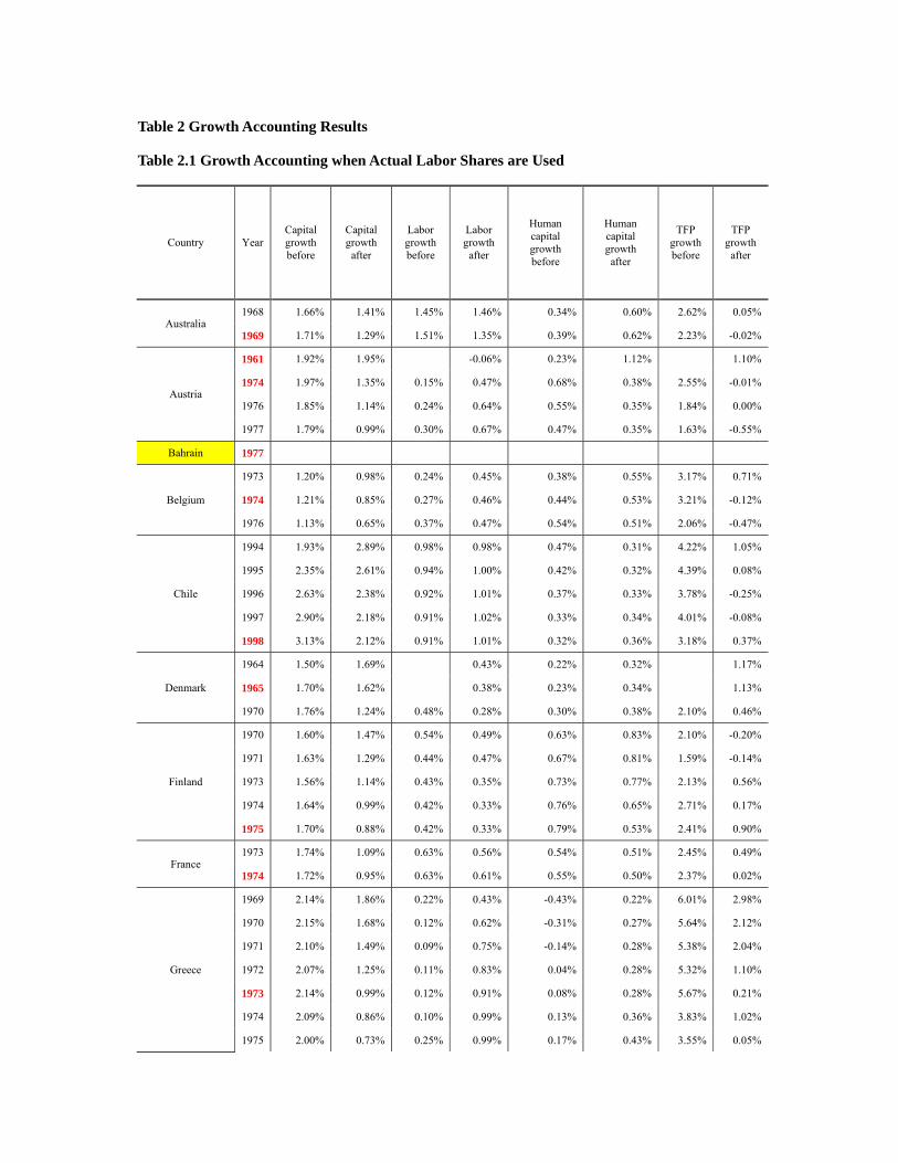
Table 2 Growth Accounting Results

Table 2.1 Growth Accounting when Actual Labor Shares are Used

Country Year Capital growth before

Capital growth

after

Labor growth before

Labor growth

after

Human capital growth before

Human capital growth

after

TFP growth before

TFP growth

after

Australia 1968 1.66% 1.41% 1.45% 1.46% 0.34% 0.60% 2.62% 0.05%

1969 1.71% 1.29% 1.51% 1.35% 0.39% 0.62% 2.23% -0.02%

Austria

1961 1.92% 1.95% -0.06% 0.23% 1.12% 1.10%

1974 1.97% 1.35% 0.15% 0.47% 0.68% 0.38% 2.55% -0.01%

1976 1.85% 1.14% 0.24% 0.64% 0.55% 0.35% 1.84% 0.00%

1977 1.79% 0.99% 0.30% 0.67% 0.47% 0.35% 1.63% -0.55%

Bahrain 1977

Belgium

1973 1.20% 0.98% 0.24% 0.45% 0.38% 0.55% 3.17% 0.71%

1974 1.21% 0.85% 0.27% 0.46% 0.44% 0.53% 3.21% -0.12%

1976 1.13% 0.65% 0.37% 0.47% 0.54% 0.51% 2.06% -0.47%

Chile

1994 1.93% 2.89% 0.98% 0.98% 0.47% 0.31% 4.22% 1.05%

1995 2.35% 2.61% 0.94% 1.00% 0.42% 0.32% 4.39% 0.08%

1996 2.63% 2.38% 0.92% 1.01% 0.37% 0.33% 3.78% -0.25%

1997 2.90% 2.18% 0.91% 1.02% 0.33% 0.34% 4.01% -0.08%

1998 3.13% 2.12% 0.91% 1.01% 0.32% 0.36% 3.18% 0.37%

Denmark

1964 1.50% 1.69% 0.43% 0.22% 0.32% 1.17%

1965 1.70% 1.62% 0.38% 0.23% 0.34% 1.13%

1970 1.76% 1.24% 0.48% 0.28% 0.30% 0.38% 2.10% 0.46%

Finland

1970 1.60% 1.47% 0.54% 0.49% 0.63% 0.83% 2.10% -0.20%

1971 1.63% 1.29% 0.44% 0.47% 0.67% 0.81% 1.59% -0.14%

1973 1.56% 1.14% 0.43% 0.35% 0.73% 0.77% 2.13% 0.56%

1974 1.64% 0.99% 0.42% 0.33% 0.76% 0.65% 2.71% 0.17%

1975 1.70% 0.88% 0.42% 0.33% 0.79% 0.53% 2.41% 0.90%

France 1973 1.74% 1.09% 0.63% 0.56% 0.54% 0.51% 2.45% 0.49%

1974 1.72% 0.95% 0.63% 0.61% 0.55% 0.50% 2.37% 0.02%

Greece

1969 2.14% 1.86% 0.22% 0.43% -0.43% 0.22% 6.01% 2.98%

1970 2.15% 1.68% 0.12% 0.62% -0.31% 0.27% 5.64% 2.12%

1971 2.10% 1.49% 0.09% 0.75% -0.14% 0.28% 5.38% 2.04%

1972 2.07% 1.25% 0.11% 0.83% 0.04% 0.28% 5.32% 1.10%

1973 2.14% 0.99% 0.12% 0.91% 0.08% 0.28% 5.67% 0.21%

1974 2.09% 0.86% 0.10% 0.99% 0.13% 0.36% 3.83% 1.02%

1975 2.00% 0.73% 0.25% 0.99% 0.17% 0.43% 3.55% 0.05%

1976 1.86% 0.58% 0.43% 0.95% 0.22% 0.50% 2.98% -1.03%

1977 1.68% 0.47% 0.62% 0.89% 0.27% 0.57% 2.12% -0.96%

1978 1.49% 0.37% 0.75% 0.84% 0.28% 0.64% 2.04% -1.45%

Hong Kong

1978 3.48% 3.75% 2.05% 1.54% 0.55% 0.62% 2.47% 0.80%

1988 3.00% 2.95% 0.82% 0.96% 0.59% 0.28% 2.31% 0.40%

1989 2.81% 3.03% 0.73% 1.13% 0.59% 0.21% 2.40% 0.51%

1990 2.77% 3.14% 0.65% 1.23% 0.59% 0.14% 2.54% 0.42%

1991 2.76% 3.07% 0.66% 1.21% 0.54% 0.13% 2.43% -1.26%

1992 2.84% 2.84% 0.68% 1.18% 0.48% 0.12% 3.01% -1.42%

1993 2.85% 2.72% 0.73% 1.12% 0.41% 0.11% 2.47% -1.01%

1994 2.90% 2.46% 0.82% 1.01% 0.34% 0.14% 1.50% -1.44%

Ireland

1969 1.26% 1.51% 0.36% 1.07% 0.19% 0.55% 3.08% 0.53%

1973 1.58% 1.45% 0.67% 1.24% 0.33% 0.61% 3.41% 0.45%

1974 1.67% 1.39% 0.79% 1.22% 0.40% 0.62% 2.78% 0.70%

1978 1.53% 1.16% 1.22% 0.96% 0.62% 0.64% 1.96% -1.41%

1979 1.56% 0.95% 1.27% 0.79% 0.61% 0.61% 1.62% -1.92%

1999 1.26% 1.75% 1.24% 1.13% 0.61% 0.44% 5.08% 2.51%

2000 1.51% 1.67% 1.26% 1.05% 0.62% 0.41% 5.78% 2.06%

Israel

1970 1.91% 2.26% 2.05% 1.62% 0.42% 0.68% 3.03% 0.36%

1971 1.95% 2.00% 1.96% 1.47% 0.47% 0.69% 3.17% -0.06%

1972 2.05% 1.75% 1.92% 1.36% 0.52% 0.70% 3.63% -0.47%

1973 2.25% 1.46% 1.94% 1.28% 0.55% 0.70% 4.89% -1.32%

1974 2.49% 1.21% 1.94% 1.21% 0.57% 0.67% 5.47% -0.93%

1975 2.57% 1.03% 1.88% 1.20% 0.60% 0.64% 3.32% -0.81%

1996 1.96% 1.31% 2.65% 1.76% 0.34% 0.33% 2.11% -1.17%

Italy 1974 1.63% 1.00% 0.24% 0.45% 0.35% 0.46% 2.90% 0.72%

Japan

1967 4.22% 4.08% 1.36% 0.76% 0.09% 0.52% 3.98% 2.38%

1968 4.18% 3.76% 1.28% 0.72% 0.10% 0.62% 4.13% 1.15%

1969 4.22% 3.41% 1.18% 0.68% 0.10% 0.68% 4.70% 0.32%

1970 4.31% 3.01% 1.06% 0.65% 0.10% 0.74% 5.08% -0.28%

1971 4.26% 2.72% 0.95% 0.62% 0.21% 0.69% 4.09% 0.26%

1972 4.28% 2.47% 0.86% 0.59% 0.32% 0.64% 4.49% 0.20%

1973 4.27% 2.18% 0.81% 0.57% 0.42% 0.59% 4.12% -0.28%

1974 4.08% 2.00% 0.76% 0.55% 0.52% 0.56% 2.38% 0.63%

1975 3.76% 1.88% 0.72% 0.54% 0.62% 0.52% 1.15% 0.81%

1990 1.51% 1.21% 0.63% 0.10% 0.45% 0.38% 2.15% -0.24%

1991 1.60% 1.06% 0.59% 0.04% 0.42% 0.38% 2.17% -0.87%

1992 1.62% 0.92% 0.53% -0.02% 0.40% 0.38% 1.54% -0.86%

Korea, Republic of 1990 3.72% 3.72% 1.38% 0.90% 0.73% 0.70% 3.81% 1.41%

1991 3.88% 3.22% 1.34% 0.82% 0.73% 0.65% 3.74% -1.19%

1992 3.98% 2.93% 1.31% 0.74% 0.73% 0.60% 3.41% 0.24%

1993 4.02% 2.71% 1.25% 0.67% 0.74% 0.56% 2.93% 0.87%

1994 4.04% 2.42% 1.16% 0.61% 0.75% 0.51% 2.76% 0.38%

1995 4.01% 2.14% 1.07% 0.54% 0.76% 0.46% 2.50% 0.45%

1996 3.95% 1.86% 0.98% 0.47% 0.73% 0.46% 2.48% 0.09%

1997 3.72% 1.69% 0.90% 0.41% 0.70% 0.45% 1.41% 0.62%

Malaysia

1994 3.07% 2.47% 1.79% 1.89% 0.84% 0.52% 3.30% 0.67%

1995 3.46% 2.02% 1.78% 1.86% 0.84% 0.49% 3.03% 0.56%

1996 3.72% 1.60% 1.79% 1.80% 0.78% 0.51% 2.83% 0.48%

1997 3.89% 1.21% 1.82% 1.74% 0.72% 0.53% 2.34% 1.02%

Mauritius 1992 2.39% 2.21% 0.86% 0.79% 0.54% 0.14% 2.42% 1.29%

Netherlands

1970 2.01% 1.26% 0.95% 0.91% 0.94% 0.60% 1.83% 0.25%

1973 1.81% 0.99% 0.86% 0.93% 0.82% 0.56% 1.32% -0.03%

1974 1.72% 0.86% 0.87% 0.95% 0.76% 0.54% 1.22% -0.76%

New Zealand

1960 1.09% 1.37% 1.49% 0.21% 0.32% 0.50%

1965 1.22% 1.06% 1.16% 0.19% 0.70% -0.49%

1966 1.37% 1.05% 1.23% 0.26% 0.72% -0.14%

Norway

1976 1.96% 1.17% 0.36% 0.39% 0.29% 0.55% 2.35% 0.23%

1997 0.52% 0.98% 0.31% 0.47% 0.36% 0.69% 3.35% 0.02%

1998 0.72% 0.96% 0.34% 0.46% 0.36% 0.76% 3.24% 0.01%

Portugal

1973 2.19% 1.36% -0.25% 1.03% 0.46% 0.68% 5.57% -0.41%

1974 2.20% 1.31% -0.05% 0.98% 0.51% 0.69% 4.65% -0.20%

1990 0.92% 1.25% 0.44% 0.46% 0.65% 0.29% 2.44% 0.45%

1991 1.09% 1.29% 0.41% 0.50% 0.59% 0.30% 3.38% 0.83%

1992 1.25% 1.34% 0.39% 0.51% 0.52% 0.32% 3.25% 1.13%

2000 1.43% 0.88% 0.48% 0.22% 0.33% 0.45% 1.84% -0.75%

Singapore

1978 4.15% 4.37% 1.73% 1.62% 0.01% 0.62% 2.59% 0.42%

1979 4.05% 4.10% 1.67% 1.48% -0.02% 0.69% 2.18% -0.65%

1980 4.05% 3.80% 1.58% 1.48% -0.05% 0.76% 1.59% -0.65%

1982 4.05% 3.14% 1.92% 1.20% 0.20% 0.60% 2.49% 0.80%

1983 4.19% 2.90% 1.82% 1.30% 0.34% 0.53% 2.74% 1.00%

1984 4.42% 2.63% 1.77% 1.34% 0.48% 0.51% 2.39% 1.46%

1993 2.78% 3.40% 1.57% 1.34% 0.56% 0.68% 4.54% 2.06%

1994 2.89% 3.21% 1.56% 1.32% 0.61% 0.64% 4.86% -0.02%

1995 3.11% 2.89% 1.51% 1.25% 0.67% 0.60% 4.44% -0.47%

1996 3.32% 2.33% 1.48% 1.16% 0.71% 0.57% 3.90% -0.98%

1997 3.53% 1.88% 1.48% 1.08% 0.75% 0.55% 3.56% -0.10%

Spain

1969 3.17% 2.43% 0.44% 0.61% 0.23% 0.80% 3.34% 0.94%

1972 2.84% 1.91% 0.38% 0.81% 0.42% 0.78% 2.59% -0.69%

1973 2.74% 1.68% 0.41% 0.83% 0.52% 0.74% 2.60% -1.29%

1974 2.70% 1.38% 0.45% 0.85% 0.63% 0.68% 2.80% -1.97%

1975 2.61% 1.17% 0.52% 0.85% 0.74% 0.62% 1.83% -1.52%

1976 2.43% 0.98% 0.61% 0.83% 0.80% 0.59% 0.94% -1.55%

1990 1.11% 1.06% 0.68% 0.37% 0.45% 1.39% 1.96% -0.99%

Trinidad &Tobago 1978 2.59% 2.20% 1.85% 1.38% 0.55% 0.32% 0.97% -5.63%

1980 3.10% 1.23% 1.83% 1.16% 0.54% 0.24% -0.41% -6.62%

United Kingdom 1988 0.62% 0.65% 0.33% 0.09% 0.21% 0.27% 2.70% 0.54%

1989 0.72% 0.59% 0.29% 0.12% 0.22% 0.29% 2.73% 0.62%

United States 1968 0.99% 0.97% 1.14% 1.34% 0.77% 0.72% 2.31% -0.55%

Uruguay

1996 0.92% 0.70% 0.43% 0.36% 0.23% 0.18% 2.71% -2.61%

1997 1.18% 0.51% 0.42% 0.36% 0.25% 0.12% 3.15% -1.58%

1998 1.42% 0.30% 0.41% 0.37% 0.27% 0.05% 3.02% -1.30%

Venezuela 1974 2.60% 2.45% 2.09% 2.07% 0.59% 0.71% 1.99% -4.39%

Average (non-oil countries)

2.40% 1.79% 0.89% 0.86% 0.44% 0.51% 3.04% 0.09%

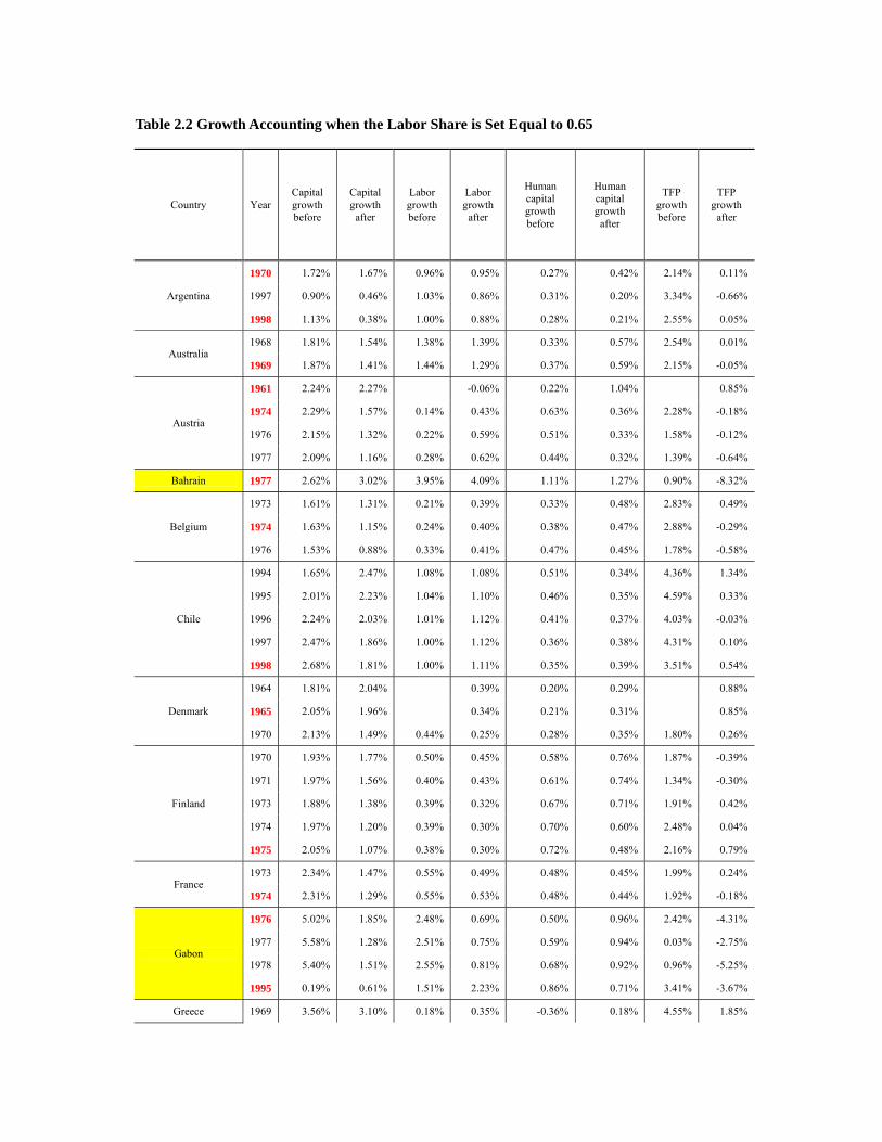
Table 2.2 Growth Accounting when the Labor Share is Set Equal to 0.65

Country Year Capital growth before

Capital growth

after

Labor growth before

Labor growth

after

Human capital growth before

Human capital growth

after

TFP growth before

TFP growth

after

Argentina

1970 1.72% 1.67% 0.96% 0.95% 0.27% 0.42% 2.14% 0.11%

1997 0.90% 0.46% 1.03% 0.86% 0.31% 0.20% 3.34% -0.66%

1998 1.13% 0.38% 1.00% 0.88% 0.28% 0.21% 2.55% 0.05%

Australia 1968 1.81% 1.54% 1.38% 1.39% 0.33% 0.57% 2.54% 0.01%

1969 1.87% 1.41% 1.44% 1.29% 0.37% 0.59% 2.15% -0.05%

Austria

1961 2.24% 2.27% -0.06% 0.22% 1.04% 0.85%

1974 2.29% 1.57% 0.14% 0.43% 0.63% 0.36% 2.28% -0.18%

1976 2.15% 1.32% 0.22% 0.59% 0.51% 0.33% 1.58% -0.12%

1977 2.09% 1.16% 0.28% 0.62% 0.44% 0.32% 1.39% -0.64%

Bahrain 1977 2.62% 3.02% 3.95% 4.09% 1.11% 1.27% 0.90% -8.32%

Belgium

1973 1.61% 1.31% 0.21% 0.39% 0.33% 0.48% 2.83% 0.49%

1974 1.63% 1.15% 0.24% 0.40% 0.38% 0.47% 2.88% -0.29%

1976 1.53% 0.88% 0.33% 0.41% 0.47% 0.45% 1.78% -0.58%

Chile

1994 1.65% 2.47% 1.08% 1.08% 0.51% 0.34% 4.36% 1.34%

1995 2.01% 2.23% 1.04% 1.10% 0.46% 0.35% 4.59% 0.33%

1996 2.24% 2.03% 1.01% 1.12% 0.41% 0.37% 4.03% -0.03%

1997 2.47% 1.86% 1.00% 1.12% 0.36% 0.38% 4.31% 0.10%

1998 2.68% 1.81% 1.00% 1.11% 0.35% 0.39% 3.51% 0.54%

Denmark

1964 1.81% 2.04% 0.39% 0.20% 0.29% 0.88%

1965 2.05% 1.96% 0.34% 0.21% 0.31% 0.85%

1970 2.13% 1.49% 0.44% 0.25% 0.28% 0.35% 1.80% 0.26%

Finland

1970 1.93% 1.77% 0.50% 0.45% 0.58% 0.76% 1.87% -0.39%

1971 1.97% 1.56% 0.40% 0.43% 0.61% 0.74% 1.34% -0.30%

1973 1.88% 1.38% 0.39% 0.32% 0.67% 0.71% 1.91% 0.42%

1974 1.97% 1.20% 0.39% 0.30% 0.70% 0.60% 2.48% 0.04%

1975 2.05% 1.07% 0.38% 0.30% 0.72% 0.48% 2.16% 0.79%

France 1973 2.34% 1.47% 0.55% 0.49% 0.48% 0.45% 1.99% 0.24%

1974 2.31% 1.29% 0.55% 0.53% 0.48% 0.44% 1.92% -0.18%

Gabon

1976 5.02% 1.85% 2.48% 0.69% 0.50% 0.96% 2.42% -4.31%

1977 5.58% 1.28% 2.51% 0.75% 0.59% 0.94% 0.03% -2.75%

1978 5.40% 1.51% 2.55% 0.81% 0.68% 0.92% 0.96% -5.25%

1995 0.19% 0.61% 1.51% 2.23% 0.86% 0.71% 3.41% -3.67%

Greece 1969 3.56% 3.10% 0.18% 0.35% -0.36% 0.18% 4.55% 1.85%

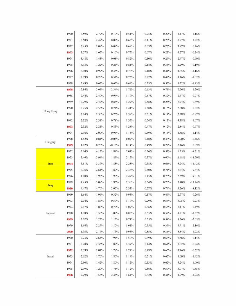
1970 3.59% 2.79% 0.10% 0.51% -0.25% 0.22% 4.17% 1.16%

1971 3.50% 2.49% 0.07% 0.62% -0.11% 0.23% 3.97% 1.22%

1972 3.45% 2.08% 0.09% 0.69% 0.03% 0.23% 3.97% 0.46%

1973 3.57% 1.65% 0.10% 0.75% 0.07% 0.23% 4.27% -0.24%

1974 3.48% 1.43% 0.08% 0.82% 0.10% 0.29% 2.47% 0.69%

1975 3.33% 1.22% 0.21% 0.81% 0.14% 0.36% 2.29% -0.19%

1976 3.10% 0.97% 0.35% 0.78% 0.18% 0.41% 1.85% -1.16%

1977 2.79% 0.78% 0.51% 0.73% 0.22% 0.47% 1.16% -1.02%

1978 2.49% 0.62% 0.62% 0.69% 0.23% 0.53% 1.22% -1.43%

Hong Kong

1978 2.84% 3.05% 2.34% 1.76% 0.63% 0.71% 2.76% 1.20%

1988 2.44% 2.40% 0.94% 1.10% 0.67% 0.32% 2.67% 0.77%

1989 2.29% 2.47% 0.84% 1.29% 0.68% 0.24% 2.74% 0.89%

1990 2.25% 2.56% 0.74% 1.41% 0.68% 0.15% 2.88% 0.82%

1991 2.24% 2.50% 0.75% 1.38% 0.61% 0.14% 2.78% -0.87%

1992 2.32% 2.31% 0.78% 1.35% 0.54% 0.13% 3.38% -1.07%

1993 2.32% 2.21% 0.83% 1.28% 0.47% 0.12% 2.84% -0.67%

1994 2.36% 2.00% 0.93% 1.15% 0.39% 0.16% 1.88% -1.14%

Hungary 1978 1.82% 0.84% -0.06% 0.09% 0.48% 0.33% 2.90% -0.46%

1979 1.82% 0.70% -0.13% 0.14% 0.49% 0.27% 2.16% 0.09%

Iran

1972 3.64% 4.12% 1.89% 2.01% 0.36% 0.57% 6.35% -8.31%

1973 3.46% 3.94% 1.89% 2.12% 0.37% 0.60% 6.68% -14.70%

1974 3.51% 3.37% 1.88% 2.25% 0.38% 0.66% 5.24% -14.42%

1975 3.76% 2.61% 1.89% 2.38% 0.40% 0.71% 2.34% -9.34%

1976 4.08% 1.98% 1.90% 2.49% 0.45% 0.73% 2.59% -9.81%

Iraq 1979 4.45% 5.08% 1.95% 2.50% 0.54% 0.70% 7.40% -11.44%

1980 4.47% 4.70% 2.05% 2.33% 0.57% 0.74% 4.26% -8.12%

Ireland

1969 1.64% 1.96% 0.32% 0.95% 0.17% 0.49% 2.77% 0.26%

1973 2.04% 1.87% 0.59% 1.10% 0.29% 0.54% 3.05% 0.23%

1974 2.17% 1.80% 0.70% 1.09% 0.36% 0.55% 2.41% 0.49%

1978 1.98% 1.50% 1.09% 0.85% 0.55% 0.57% 1.71% -1.57%

1979 2.02% 1.23% 1.13% 0.71% 0.55% 0.54% 1.36% -2.05%

1999 1.64% 2.27% 1.10% 1.01% 0.55% 0.39% 4.91% 2.16%

2000 1.95% 2.17% 1.13% 0.93% 0.55% 0.36% 5.54% 1.72%

Israel

1970 2.23% 2.64% 1.91% 1.50% 0.39% 0.63% 2.88% 0.14%

1971 2.28% 2.33% 1.82% 1.37% 0.44% 0.64% 3.02% -0.24%

1972 2.39% 2.04% 1.78% 1.27% 0.49% 0.65% 3.46% -0.62%

1973 2.62% 1.70% 1.80% 1.19% 0.51% 0.65% 4.69% -1.42%

1974 2.90% 1.42% 1.80% 1.12% 0.53% 0.62% 5.24% -1.00%

1975 2.99% 1.20% 1.75% 1.12% 0.56% 0.59% 3.07% -0.85%

1996 2.29% 1.53% 2.46% 1.64% 0.32% 0.31% 1.99% -1.24%

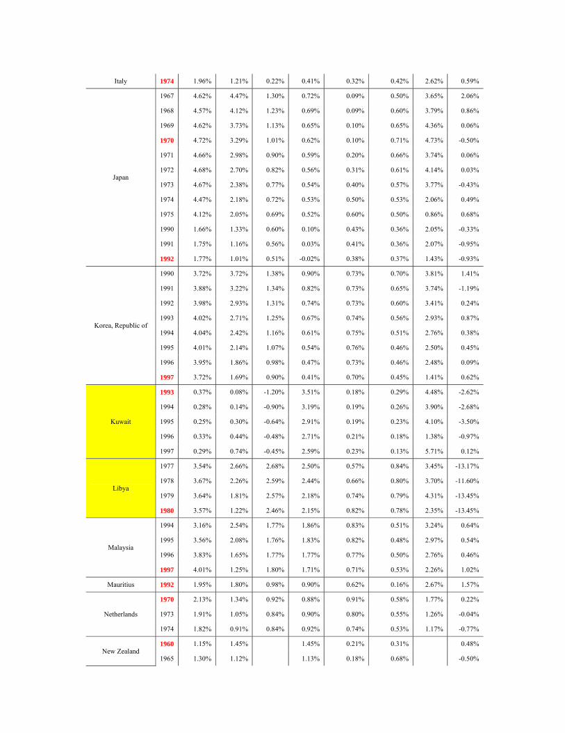
Italy 1974 1.96% 1.21% 0.22% 0.41% 0.32% 0.42% 2.62% 0.59%

Japan

1967 4.62% 4.47% 1.30% 0.72% 0.09% 0.50% 3.65% 2.06%

1968 4.57% 4.12% 1.23% 0.69% 0.09% 0.60% 3.79% 0.86%

1969 4.62% 3.73% 1.13% 0.65% 0.10% 0.65% 4.36% 0.06%

1970 4.72% 3.29% 1.01% 0.62% 0.10% 0.71% 4.73% -0.50%

1971 4.66% 2.98% 0.90% 0.59% 0.20% 0.66% 3.74% 0.06%

1972 4.68% 2.70% 0.82% 0.56% 0.31% 0.61% 4.14% 0.03%

1973 4.67% 2.38% 0.77% 0.54% 0.40% 0.57% 3.77% -0.43%

1974 4.47% 2.18% 0.72% 0.53% 0.50% 0.53% 2.06% 0.49%

1975 4.12% 2.05% 0.69% 0.52% 0.60% 0.50% 0.86% 0.68%

1990 1.66% 1.33% 0.60% 0.10% 0.43% 0.36% 2.05% -0.33%

1991 1.75% 1.16% 0.56% 0.03% 0.41% 0.36% 2.07% -0.95%

1992 1.77% 1.01% 0.51% -0.02% 0.38% 0.37% 1.43% -0.93%

Korea, Republic of

1990 3.72% 3.72% 1.38% 0.90% 0.73% 0.70% 3.81% 1.41%

1991 3.88% 3.22% 1.34% 0.82% 0.73% 0.65% 3.74% -1.19%

1992 3.98% 2.93% 1.31% 0.74% 0.73% 0.60% 3.41% 0.24%

1993 4.02% 2.71% 1.25% 0.67% 0.74% 0.56% 2.93% 0.87%

1994 4.04% 2.42% 1.16% 0.61% 0.75% 0.51% 2.76% 0.38%

1995 4.01% 2.14% 1.07% 0.54% 0.76% 0.46% 2.50% 0.45%

1996 3.95% 1.86% 0.98% 0.47% 0.73% 0.46% 2.48% 0.09%

1997 3.72% 1.69% 0.90% 0.41% 0.70% 0.45% 1.41% 0.62%

Kuwait

1993 0.37% 0.08% -1.20% 3.51% 0.18% 0.29% 4.48% -2.62%

1994 0.28% 0.14% -0.90% 3.19% 0.19% 0.26% 3.90% -2.68%

1995 0.25% 0.30% -0.64% 2.91% 0.19% 0.23% 4.10% -3.50%

1996 0.33% 0.44% -0.48% 2.71% 0.21% 0.18% 1.38% -0.97%

1997 0.29% 0.74% -0.45% 2.59% 0.23% 0.13% 5.71% 0.12%

Libya

1977 3.54% 2.66% 2.68% 2.50% 0.57% 0.84% 3.45% -13.17%

1978 3.67% 2.26% 2.59% 2.44% 0.66% 0.80% 3.70% -11.60%

1979 3.64% 1.81% 2.57% 2.18% 0.74% 0.79% 4.31% -13.45%

1980 3.57% 1.22% 2.46% 2.15% 0.82% 0.78% 2.35% -13.45%

Malaysia

1994 3.16% 2.54% 1.77% 1.86% 0.83% 0.51% 3.24% 0.64%

1995 3.56% 2.08% 1.76% 1.83% 0.82% 0.48% 2.97% 0.54%

1996 3.83% 1.65% 1.77% 1.77% 0.77% 0.50% 2.76% 0.46%

1997 4.01% 1.25% 1.80% 1.71% 0.71% 0.53% 2.26% 1.02%

Mauritius 1992 1.95% 1.80% 0.98% 0.90% 0.62% 0.16% 2.67% 1.57%

Netherlands

1970 2.13% 1.34% 0.92% 0.88% 0.91% 0.58% 1.77% 0.22%

1973 1.91% 1.05% 0.84% 0.90% 0.80% 0.55% 1.26% -0.04%

1974 1.82% 0.91% 0.84% 0.92% 0.74% 0.53% 1.17% -0.77%

New Zealand 1960 1.15% 1.45% 1.45% 0.21% 0.31% 0.48%

1965 1.30% 1.12% 1.13% 0.18% 0.68% -0.50%

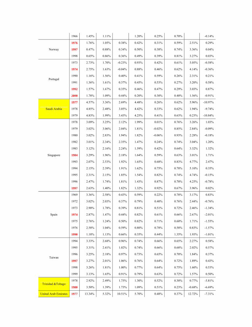
1966 1.45% 1.11% 1.20% 0.25% 0.70% -0.14%

Norway

1976 1.76% 1.05% 0.38% 0.42% 0.31% 0.59% 2.51% 0.29%

1997 0.47% 0.88% 0.34% 0.50% 0.38% 0.74% 3.36% 0.04%

1998 0.65% 0.86% 0.36% 0.49% 0.39% 0.81% 3.27% 0.03%

Portugal

1973 2.73% 1.70% -0.23% 0.93% 0.42% 0.61% 5.05% -0.58%

1974 2.75% 1.63% -0.04% 0.88% 0.46% 0.62% 4.14% -0.36%

1990 1.16% 1.56% 0.40% 0.41% 0.59% 0.26% 2.31% 0.21%

1991 1.36% 1.61% 0.37% 0.45% 0.53% 0.27% 3.20% 0.58%

1992 1.57% 1.67% 0.35% 0.46% 0.47% 0.29% 3.03% 0.87%

2000 1.78% 1.09% 0.44% 0.20% 0.30% 0.40% 1.56% -0.91%

Saudi Arabia

1977 4.57% 3.36% 2.69% 4.48% 0.26% 0.62% 5.96% -10.97%

1978 4.85% 2.48% 3.05% 4.42% 0.33% 0.62% 1.94% -9.74%

1979 4.83% 1.99% 3.43% 4.25% 0.41% 0.63% 0.23% -10.84%

Singapore

1978 3.09% 3.25% 2.12% 1.99% 0.01% 0.76% 3.26% 1.03%

1979 3.02% 3.06% 2.04% 1.81% -0.02% 0.85% 2.84% -0.09%

1980 3.02% 2.83% 1.94% 1.82% -0.06% 0.93% 2.28% -0.18%

1982 3.01% 2.34% 2.35% 1.47% 0.24% 0.74% 3.04% 1.20%

1983 3.12% 2.16% 2.24% 1.59% 0.42% 0.64% 3.32% 1.32%

1984 3.29% 1.96% 2.18% 1.64% 0.59% 0.63% 3.01% 1.71%

1993 2.07% 2.53% 1.92% 1.65% 0.68% 0.83% 4.77% 2.47%

1994 2.15% 2.39% 1.91% 1.62% 0.75% 0.78% 5.10% 0.35%

1995 2.31% 2.15% 1.85% 1.54% 0.82% 0.74% 4.74% -0.15%

1996 2.47% 1.74% 1.81% 1.43% 0.87% 0.70% 4.25% -0.78%

1997 2.63% 1.40% 1.82% 1.32% 0.92% 0.67% 3.96% 0.02%

Spain

1969 3.36% 2.58% 0.43% 0.59% 0.22% 0.78% 3.17% 0.83%

1972 3.02% 2.03% 0.37% 0.79% 0.40% 0.76% 2.44% -0.76%

1973 2.90% 1.78% 0.39% 0.81% 0.51% 0.72% 2.46% -1.34%

1974 2.87% 1.47% 0.44% 0.82% 0.61% 0.66% 2.67% -2.01%

1975 2.76% 1.24% 0.50% 0.82% 0.71% 0.60% 1.71% -1.55%

1976 2.58% 1.04% 0.59% 0.80% 0.78% 0.58% 0.83% -1.57%

1990 1.18% 1.13% 0.66% 0.35% 0.44% 1.35% 1.93% -1.01%

Taiwan

1994 3.33% 2.68% 0.96% 0.74% 0.66% 0.65% 2.27% 0.58%

1995 3.31% 2.41% 1.02% 0.74% 0.66% 0.68% 2.02% 0.57%

1996 3.25% 2.18% 0.97% 0.73% 0.65% 0.70% 1.84% 0.37%

1997 3.27% 2.01% 1.06% 0.76% 0.64% 0.72% 1.89% 0.43%

1998 3.26% 1.81% 1.00% 0.77% 0.64% 0.75% 1.60% 0.53%

1999 3.13% 1.65% 0.91% 0.79% 0.63% 0.72% 1.57% 0.50%

Trinidad &Tobago 1978 2.92% 2.49% 1.75% 1.30% 0.52% 0.30% 0.77% -5.81%

1980 3.50% 1.39% 1.73% 1.09% 0.51% 0.23% -0.68% -6.69%

United Arab Emirates 1977 13.34% 5.32% 10.51% 5.70% 0.48% 0.37% 12.72% -7.31%

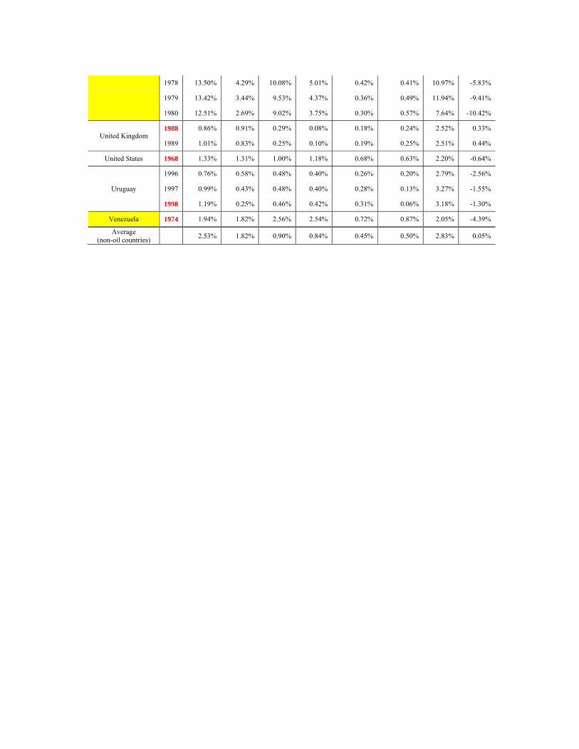
1978 13.50% 4.29% 10.08% 5.01% 0.42% 0.41% 10.97% -5.83%

1979 13.42% 3.44% 9.53% 4.37% 0.36% 0.49% 11.94% -9.41%

1980 12.51% 2.69% 9.02% 3.75% 0.30% 0.57% 7.64% -10.42%

United Kingdom 1988 0.86% 0.91% 0.29% 0.08% 0.18% 0.24% 2.52% 0.33%

1989 1.01% 0.83% 0.25% 0.10% 0.19% 0.25% 2.51% 0.44%

United States 1968 1.33% 1.31% 1.00% 1.18% 0.68% 0.63% 2.20% -0.64%

Uruguay

1996 0.76% 0.58% 0.48% 0.40% 0.26% 0.20% 2.79% -2.56%

1997 0.99% 0.43% 0.48% 0.40% 0.28% 0.13% 3.27% -1.55%

1998 1.19% 0.25% 0.46% 0.42% 0.31% 0.06% 3.18% -1.30%

Venezuela 1974 1.94% 1.82% 2.56% 2.54% 0.72% 0.87% 2.05% -4.39%

Average (non-oil countries) 2.53% 1.82% 0.90% 0.84% 0.45% 0.50% 2.83% 0.05%

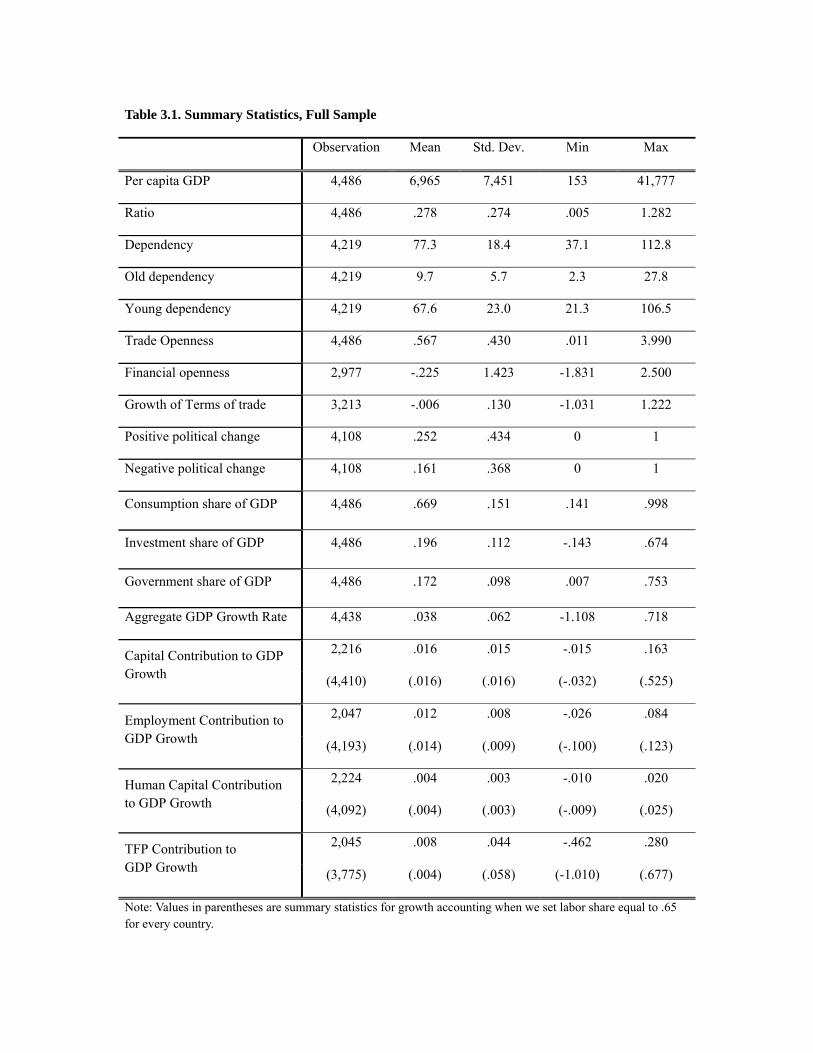
Table 3.1. Summary Statistics, Full Sample

Note: Values in parentheses are summary statistics for growth accounting when we set labor share equal to .65 for every country.

Observation Mean Std. Dev. Min Max

Per capita GDP 4,486 6,965 7,451 153 41,777

Ratio 4,486 .278 .274 .005 1.282

Dependency 4,219 77.3 18.4 37.1 112.8

Old dependency 4,219 9.7 5.7 2.3 27.8

Young dependency 4,219 67.6 23.0 21.3 106.5

Trade Openness 4,486 .567 .430 .011 3.990

Financial openness 2,977 -.225 1.423 -1.831 2.500

Growth of Terms of trade 3,213 -.006 .130 -1.031 1.222

Positive political change 4,108 .252 .434 0 1

Negative political change 4,108 .161 .368 0 1

Consumption share of GDP 4,486 .669 .151 .141 .998

Investment share of GDP 4,486 .196 .112 -.143 .674

Government share of GDP 4,486 .172 .098 .007 .753

Aggregate GDP Growth Rate 4,438 .038 .062 -1.108 .718

Capital Contribution to GDP Growth

2,216 .016 .015 -.015 .163

(4,410) (.016) (.016) (-.032) (.525)

Employment Contribution to GDP Growth

2,047 .012 .008 -.026 .084

(4,193) (.014) (.009) (-.100) (.123)

Human Capital Contribution to GDP Growth

2,224 .004 .003 -.010 .020

(4,092) (.004) (.003) (-.009) (.025)

TFP Contribution to GDP Growth

2,045 .008 .044 -.462 .280

(3,775) (.004) (.058) (-1.010) (.677)

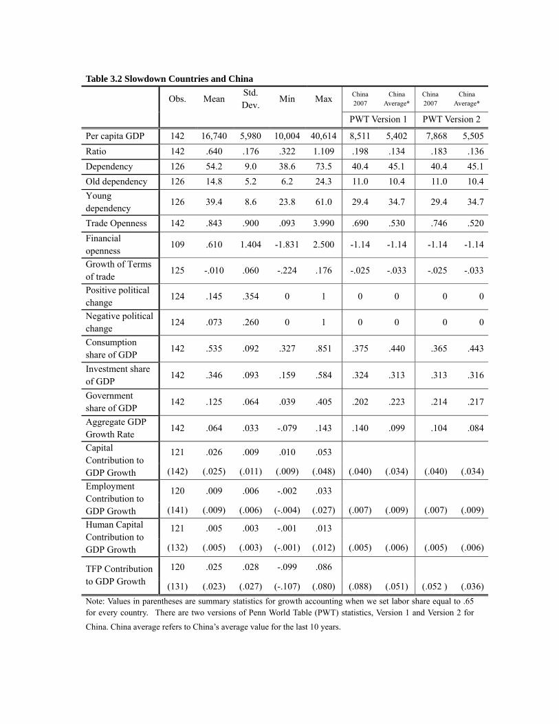
Table 3.2 Slowdown Countries and China

Note: Values in parentheses are summary statistics for growth accounting when we set labor share equal to .65 for every country. There are two versions of Penn World Table (PWT) statistics, Version 1 and Version 2 for

China. China average refers to China’s average value for the last 10 years.

Obs. Mean Std. Dev.

Min Max China 2007

China Average*

China 2007

China Average*

PWT Version 1 PWT Version 2

Per capita GDP 142 16,740 5,980 10,004 40,614 8,511 5,402 7,868 5,505

Ratio 142 .640 .176 .322 1.109 .198 .134 .183 .136

Dependency 126 54.2 9.0 38.6 73.5 40.4 45.1 40.4 45.1

Old dependency 126 14.8 5.2 6.2 24.3 11.0 10.4 11.0 10.4

Young dependency

126 39.4 8.6 23.8 61.0 29.4 34.7 29.4 34.7

Trade Openness 142 .843 .900 .093 3.990 .690 .530 .746 .520

Financial openness

109 .610 1.404 -1.831 2.500 -1.14 -1.14 -1.14 -1.14

Growth of Terms of trade

125 -.010 .060 -.224 .176 -.025 -.033 -.025 -.033

Positive political change

124 .145 .354 0 1 0 0 0 0

Negative political change

124 .073 .260 0 1 0 0 0 0

Consumption share of GDP

142 .535 .092 .327 .851 .375 .440 .365 .443

Investment share of GDP

142 .346 .093 .159 .584 .324 .313 .313 .316

Government share of GDP

142 .125 .064 .039 .405 .202 .223 .214 .217

Aggregate GDP Growth Rate

142 .064 .033 -.079 .143 .140 .099 .104 .084

Capital Contribution to GDP Growth

121 .026 .009 .010 .053

(142) (.025) (.011) (.009) (.048) (.040) (.034) (.040) (.034)

Employment Contribution to GDP Growth

120 .009 .006 -.002 .033

(141) (.009) (.006) (-.004) (.027) (.007) (.009) (.007) (.009)

Human Capital Contribution to GDP Growth

121 .005 .003 -.001 .013

(132) (.005) (.003) (-.001) (.012) (.005) (.006) (.005) (.006)

TFP Contribution to GDP Growth

120 .025 .028 -.099 .086

(131) (.023) (.027) (-.107) (.080) (.088) (.051) (.052 ) (.036)

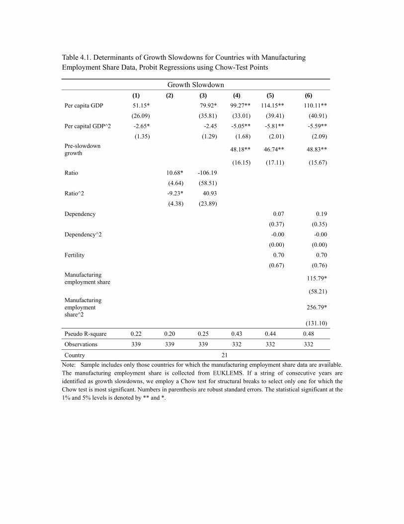
Table 4.1. Determinants of Growth Slowdowns for Countries with Manufacturing Employment Share Data, Probit Regressions using Chow-Test Points

Growth Slowdown

(1) (2) (3) (4) (5) (6)

Per capita GDP 51.15* 79.92* 99.27** 114.15** 110.11**

(26.09) (35.81) (33.01) (39.41) (40.91)

Per capital GDP^2 -2.65* -2.45 -5.05** -5.81** -5.59**

(1.35) (1.29) (1.68) (2.01) (2.09)

Pre-slowdown growth

48.18** 46.74** 48.83**

(16.15) (17.11) (15.67)

Ratio 10.68* -106.19

(4.64) (58.51)

Ratio^2 -9.23* 40.93

(4.38) (23.89)

Dependency 0.07 0.19

(0.37) (0.35)

Dependency^2 -0.00 -0.00

(0.00) (0.00)

Fertility 0.70 0.70

(0.67) (0.76)

Manufacturing employment share

115.79*

(58.21)

Manufacturing employment share^2

256.79*

(131.10)

Pseudo R-square 0.22 0.20 0.25 0.43 0.44 0.48

Observations 339 339 339 332 332 332

Country 21

Note: Sample includes only those countries for which the manufacturing employment share data are available. The manufacturing employment share is collected from EUKLEMS. If a string of consecutive years are identified as growth slowdowns, we employ a Chow test for structural breaks to select only one for which the Chow test is most significant. Numbers in parenthesis are robust standard errors. The statistical significant at the 1% and 5% levels is denoted by ** and *.

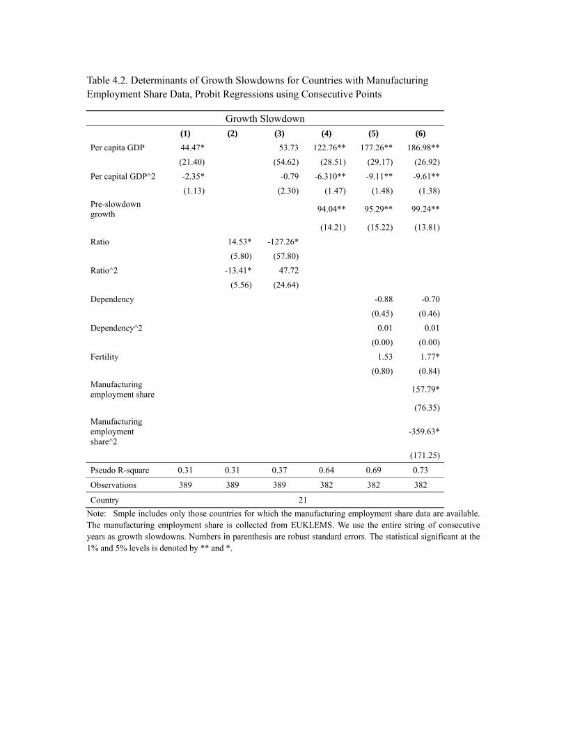
Table 4.2. Determinants of Growth Slowdowns for Countries with Manufacturing Employment Share Data, Probit Regressions using Consecutive Points

Growth Slowdown

(1) (2) (3) (4) (5) (6)

Per capita GDP 44.47* 53.73 122.76** 177.26** 186.98**

(21.40) (54.62) (28.51) (29.17) (26.92)

Per capital GDP^2 -2.35* -0.79 -6.310** -9.11** -9.61**

(1.13) (2.30) (1.47) (1.48) (1.38)

Pre-slowdown growth

94.04** 95.29** 99.24**

(14.21) (15.22) (13.81)

Ratio 14.53* -127.26*

(5.80) (57.80)

Ratio^2 -13.41* 47.72

(5.56) (24.64)

Dependency -0.88 -0.70

(0.45) (0.46)

Dependency^2 0.01 0.01

(0.00) (0.00)

Fertility 1.53 1.77*

(0.80) (0.84)

Manufacturing employment share

157.79*

(76.35)

Manufacturing employment share^2

-359.63*

(171.25)

Pseudo R-square 0.31 0.31 0.37 0.64 0.69 0.73

Observations 389 389 389 382 382 382

Country 21

Note: Smple includes only those countries for which the manufacturing employment share data are available. The manufacturing employment share is collected from EUKLEMS. We use the entire string of consecutive years as growth slowdowns. Numbers in parenthesis are robust standard errors. The statistical significant at the 1% and 5% levels is denoted by ** and *.

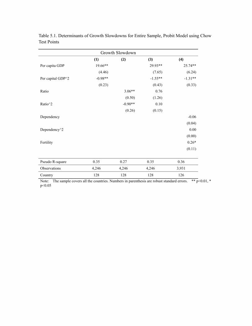
Table 5.1. Determinants of Growth Slowdowns for Entire Sample, Probit Model using Chow Test Points

Growth Slowdown

(1) (2) (3) (4)

Per capita GDP 19.66** 29.93** 25.74**

(4.46) (7.65) (6.24)

Per capital GDP^2 -0.98** -1.55** -1.31**

(0.23) (0.43) (0.33)

Ratio 3.06** 0.76

(0.50) (1.26)

Ratio^2 -0.90** 0.10

(0.26) (0.15)

Dependency -0.06

(0.04)

Dependency^2 0.00

(0.00)

Fertility 0.26*

(0.11)

Pseudo R-square 0.35 0.27 0.35 0.36

Observations 4,246 4,246 4,246 3,931

Country 128 128 128 126

Note: The sample covers all the countries. Numbers in parenthesis are robust standard errors. ** p<0.01, * p<0.05

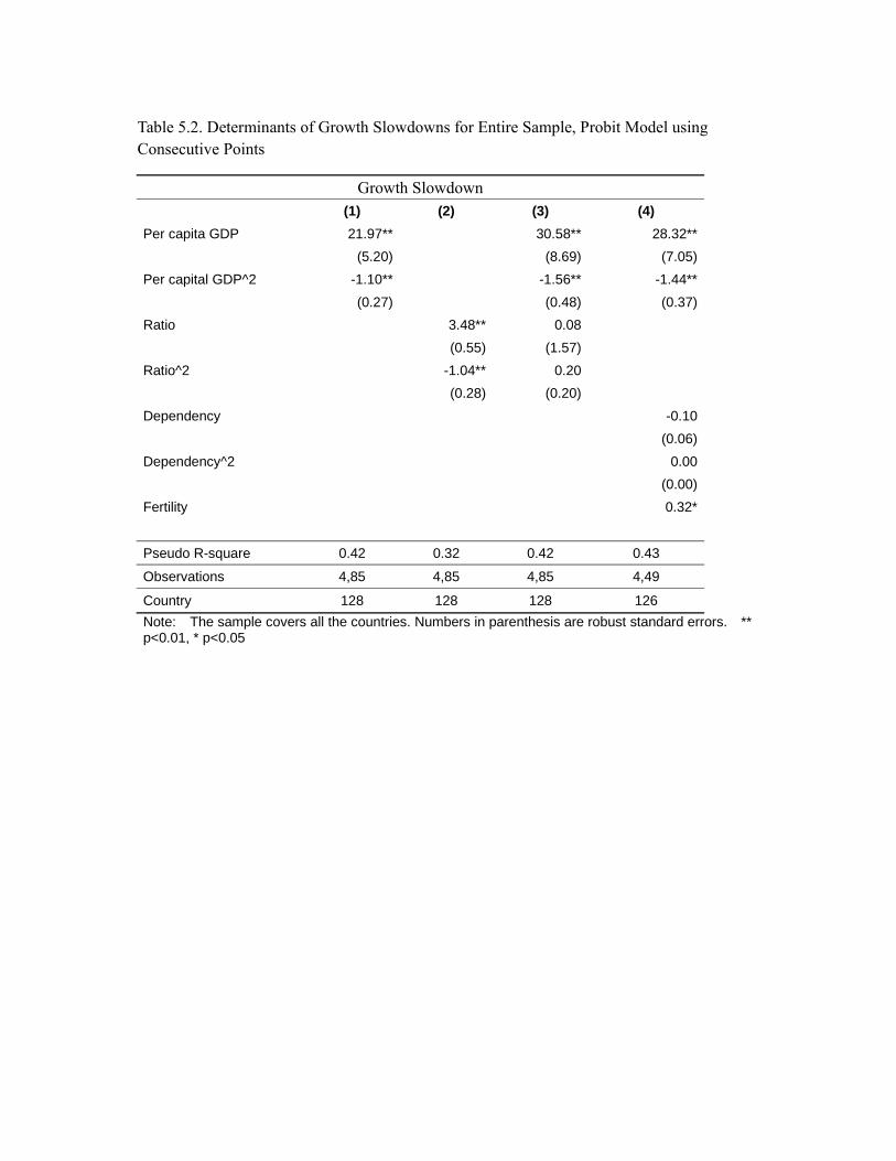
Table 5.2. Determinants of Growth Slowdowns for Entire Sample, Probit Model using Consecutive Points

Growth Slowdown

(1) (2) (3) (4)

Per capita GDP 21.97** 30.58** 28.32**

(5.20) (8.69) (7.05)

Per capital GDP^2 -1.10** -1.56** -1.44**

(0.27) (0.48) (0.37)

Ratio 3.48** 0.08

(0.55) (1.57)

Ratio^2 -1.04** 0.20

(0.28) (0.20)

Dependency -0.10

(0.06)

Dependency^2 0.00

(0.00)

Fertility 0.32*

Pseudo R-square 0.42 0.32 0.42 0.43

Observations 4,85 4,85 4,85 4,49

Country 128 128 128 126

Note: The sample covers all the countries. Numbers in parenthesis are robust standard errors. ** p<0.01, * p<0.05

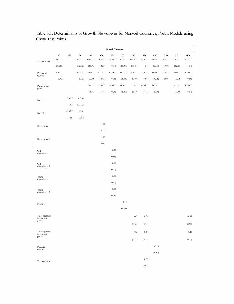
Table 6.1. Determinants of Growth Slowdowns for Non-oil Countries, Probit Models using Chow Test Points

Growth Slowdown

(1) (2) (3) (4) (5) (6) (7) (8) (9) (10) (11) (12) (13)

Per capita GDP 48.19**

50.53** 60.63** 60.83** 61.63** 62.59** 60.59** 60.05** 60.63** 54.07** 75.58** 77.27**

(13.25)

(12.52) (13.96) (14.33) (17.04) (15.35) (13.44) (15.36) (15.98) (17.98) (12.25) (11.54)

Per capital GDP^2

-2.47**

-2.12** -3.08** -3.08** -3.14** -3.17** -3.07** -3.05** -3.06** -2.79** -3.84** -3.93**

(0.70)

(0.63) (0.73) (0.75) (0.88) (0.80) (0.70) (0.80) (0.84) (0.95) (0.64) (0.60)

Pre-slowdown growth

35.03** 39.19** 51.96** 36.70** 37.50** 40.91** 38.13**

42.53** 43.50**

(4.75) (5.77) (10.29) (5.31) (6.10) (7.45) (5.53)

(7.83) (7.54)

Ratio

9.88** -29.03

(1.67) (17.50)

Ratio^2

-6.87** 10.41

(1.58) (7.09)

Dependency

0.17

(0.12)

Dependency^2

-0.00

(0.00)

Old dependency

0.29

(0.16)

Old dependency^2

-0.01

(0.01)

Young dependency

0.06

(0.11)

Young dependency^2

-0.00

(0.00)

Fertility

0.14

(0.16)

Trade openness in constant prices

0.02 -0.24

-0.49

(0.53) (0.50)

(0.62)

Trade openness in constant prices^2

-0.05 0.04

0.11

(0.16) (0.15)

(0.21)

Financial openness

-0.10

(0.10)

Terms of trade

0.56

(0.52)

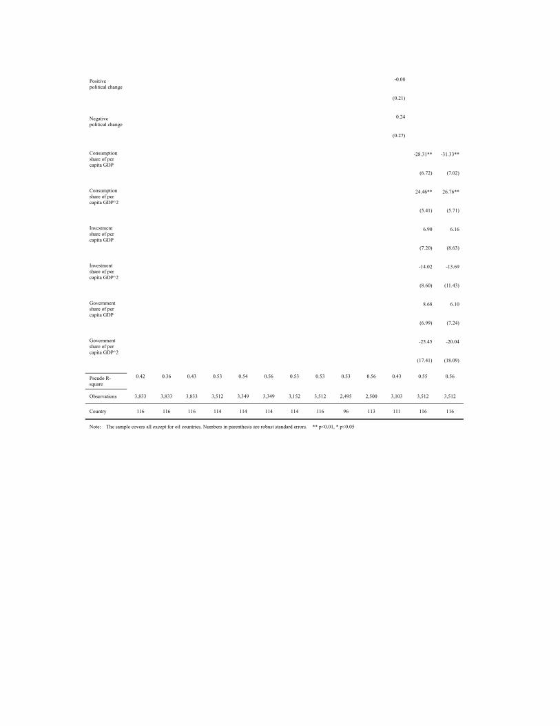
Positive political change

-0.08

(0.21)

Negative political change

0.24

(0.27)

Consumption share of per capita GDP

-28.31** -31.33**

(6.72) (7.02)

Consumption share of per capita GDP^2

24.46** 26.76**

(5.41) (5.71)

Investment share of per capita GDP

6.90 6.16

(7.20) (8.63)

Investment share of per capita GDP^2

-14.02 -13.69

(8.60) (11.43)

Government share of per capita GDP

8.68 6.10

(6.99) (7.24)

Government share of per capita GDP^2

-25.45 -20.04

(17.41) (18.09)

Pseudo R-square

0.42 0.36 0.43 0.53 0.54 0.56 0.53 0.53 0.53 0.56 0.43 0.55 0.56

Observations 3,833 3,833 3,833 3,512 3,349 3,349 3,152 3,512 2,495 2,500 3,103 3,512 3,512

Country 116 116 116 114 114 114 114 116 96 113 111 116 116

Note: The sample covers all except for oil countries. Numbers in parenthesis are robust standard errors. ** p<0.01, * p<0.05

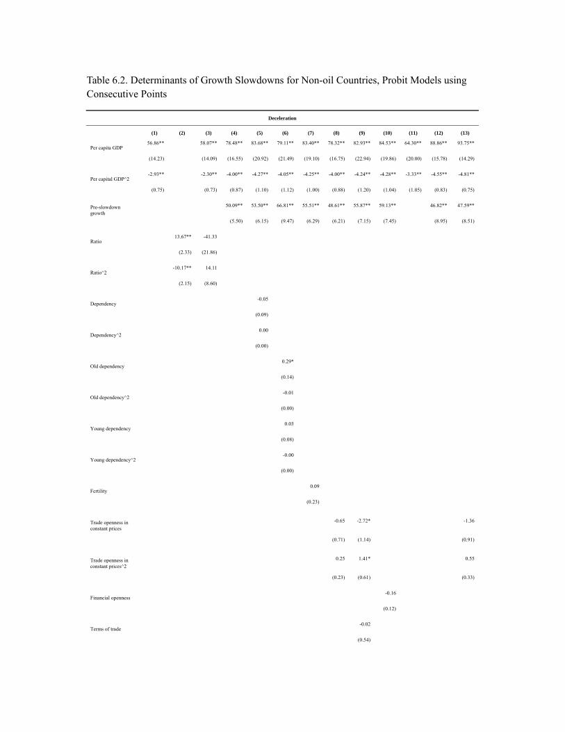
Table 6.2. Determinants of Growth Slowdowns for Non-oil Countries, Probit Models using Consecutive Points

Deceleration

(1) (2) (3) (4) (5) (6) (7) (8) (9) (10) (11) (12) (13)

Per capita GDP 56.86**

58.07** 78.48** 83.68** 79.11** 83.40** 78.32** 82.93** 84.53** 64.30** 88.86** 93.75**

(14.23)

(14.09) (16.55) (20.92) (21.49) (19.10) (16.75) (22.94) (19.86) (20.00) (15.78) (14.29)

Per capital GDP^2 -2.93**

-2.30** -4.00** -4.27** -4.05** -4.25** -4.00** -4.24** -4.28** -3.33** -4.55** -4.81**

(0.75)

(0.73) (0.87) (1.10) (1.12) (1.00) (0.88) (1.20) (1.04) (1.05) (0.83) (0.75)

Pre-slowdown growth

50.09** 53.50** 66.81** 55.51** 48.61** 55.87** 59.13**

46.82** 47.59**

(5.50) (6.15) (9.47) (6.29) (6.21) (7.15) (7.45)

(8.95) (8.51)

Ratio

13.67** -41.33

(2.33) (21.86)

Ratio^2

-10.17** 14.11

(2.15) (8.60)

Dependency

-0.05

(0.09)

Dependency^2

0.00

(0.00)

Old dependency

0.29*

(0.14)

Old dependency^2

-0.01

(0.00)

Young dependency

0.03

(0.08)

Young dependency^2

-0.00

(0.00)

Fertility

0.09

(0.23)

Trade openness in constant prices

-0.65 -2.72*

-1.36

(0.71) (1.14)

(0.91)

Trade openness in constant prices^2

0.25 1.41*

0.55

(0.23) (0.61)

(0.33)

Financial openness

-0.16

(0.12)

Terms of trade

-0.02

(0.54)

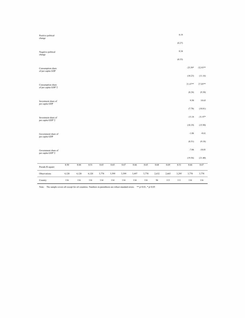
Positive political change

0.19

(0.27)

Negative political change

0.34

(0.33)

Consumption share of per capita GDP

-25.59* -32.93**

(10.23) (11.16)

Consumption share of per capita GDP^2

21.47** 27.05**

(8.24) (9.30)

Investment share of per capita GDP

9.50 18.63

(7.78) (10.81)

Investment share of per capita GDP^2

-15.18 -31.97*

(10.19) (15.90)

Government share of per capita GDP

-1.06 -0.61

(8.51) (9.18)

Government share of per capita GDP^2

-7.06 -10.01

(19.56) (21.40)

Pseudo R-square 0.50 0.44 0.51 0.65 0.65 0.67 0.66 0.65 0.68 0.69 0.51 0.66 0.67

Observations 4,120 4,120 4,120 3,770 3,599 3,599 3,497 3,770 2,632 2,665 3,295 3,770 3,770

Country 116 116 116 114 114 114 114 116 96 113 111 116 116

Note: The sample covers all except for oil countries. Numbers in parenthesis are robust standard errors. ** p<0.01, * p<0.05

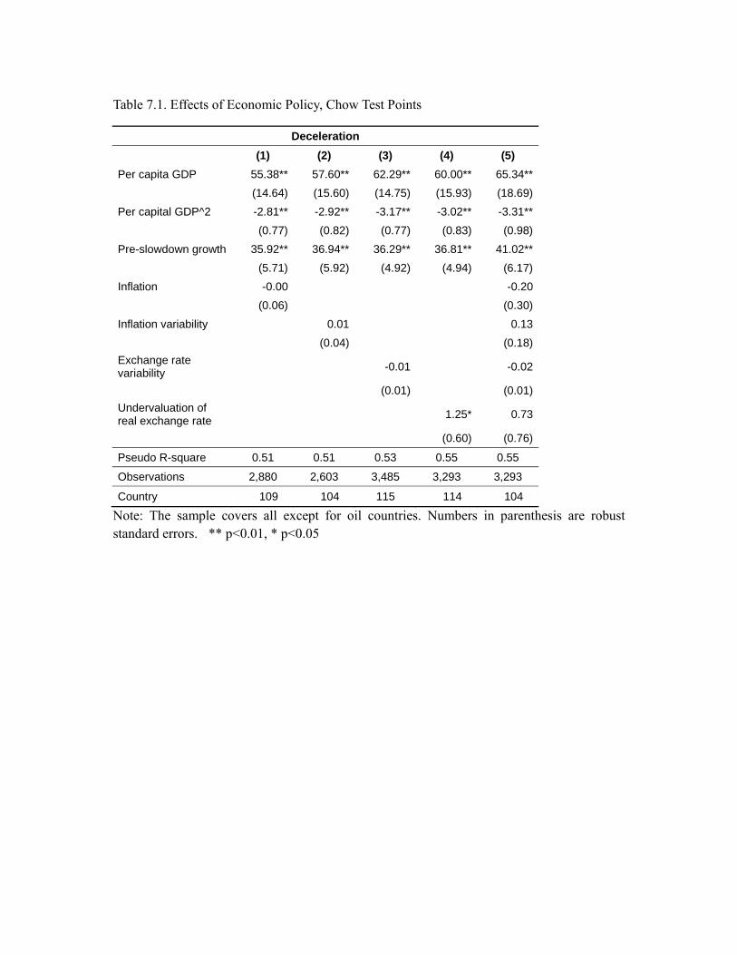
Table 7.1. Effects of Economic Policy, Chow Test Points

Deceleration

(1) (2) (3) (4) (5)

Per capita GDP 55.38** 57.60** 62.29** 60.00** 65.34**

(14.64) (15.60) (14.75) (15.93) (18.69)

Per capital GDP^2 -2.81** -2.92** -3.17** -3.02** -3.31**

(0.77) (0.82) (0.77) (0.83) (0.98)

Pre-slowdown growth 35.92** 36.94** 36.29** 36.81** 41.02**

(5.71) (5.92) (4.92) (4.94) (6.17)

Inflation -0.00 -0.20

(0.06) (0.30)

Inflation variability 0.01 0.13

(0.04) (0.18)

Exchange rate variability

-0.01 -0.02

(0.01) (0.01)

Undervaluation of real exchange rate

1.25* 0.73

(0.60) (0.76)

Pseudo R-square 0.51 0.51 0.53 0.55 0.55

Observations 2,880 2,603 3,485 3,293 3,293

Country 109 104 115 114 104

Note: The sample covers all except for oil countries. Numbers in parenthesis are robust standard errors. ** p<0.01, * p<0.05

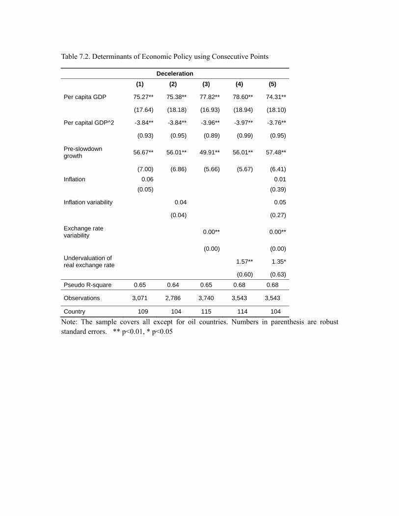
Table 7.2. Determinants of Economic Policy using Consecutive Points

Deceleration

(1) (2) (3) (4) (5)

Per capita GDP 75.27** 75.38** 77.82** 78.60** 74.31**

(17.64) (18.18) (16.93) (18.94) (18.10)

Per capital GDP^2 -3.84** -3.84** -3.96** -3.97** -3.76**

(0.93) (0.95) (0.89) (0.99) (0.95)

Pre-slowdown growth

56.67** 56.01** 49.91** 56.01** 57.48**

(7.00) (6.86) (5.66) (5.67) (6.41)

Inflation 0.06 0.01

(0.05) (0.39)

Inflation variability

0.04 0.05

(0.04) (0.27)

Exchange rate variability

0.00** 0.00**

(0.00) (0.00)

Undervaluation of real exchange rate

1.57** 1.35*

(0.60) (0.63)

Pseudo R-square 0.65 0.64 0.65 0.68 0.68

Observations 3,071 2,786 3,740 3,543 3,543

Country 109 104 115 114 104

Note: The sample covers all except for oil countries. Numbers in parenthesis are robust standard errors. ** p<0.01, * p<0.05

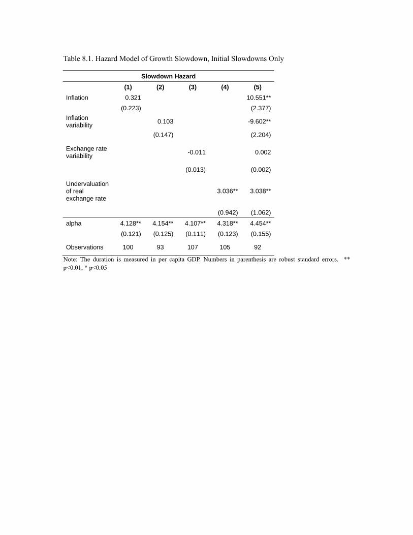
Table 8.1. Hazard Model of Growth Slowdown, Initial Slowdowns Only

Slowdown Hazard

(1) (2) (3) (4) (5)

Inflation 0.321 10.551**

(0.223) (2.377)

Inflation variability

0.103 -9.602**

(0.147) (2.204)

Exchange rate variability

-0.011 0.002

(0.013) (0.002)

Undervaluation of real exchange rate

3.036** 3.038**

(0.942) (1.062)

alpha 4.128** 4.154** 4.107** 4.318** 4.454**

(0.121) (0.125) (0.111) (0.123) (0.155)

Observations 100 93 107 105 92

Note: The duration is measured in per capita GDP. Numbers in parenthesis are robust standard errors. ** p<0.01, * p<0.05

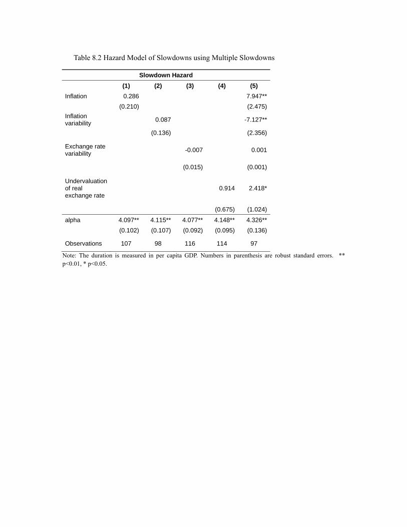
Table 8.2 Hazard Model of Slowdowns using Multiple Slowdowns

Slowdown Hazard

(1) (2) (3) (4) (5)

Inflation 0.286 7.947**

(0.210) (2.475)

Inflation variability

0.087 -7.127**

(0.136) (2.356)

Exchange rate variability

-0.007 0.001

(0.015) (0.001)

Undervaluation of real exchange rate

0.914 2.418*

(0.675) (1.024)

alpha 4.097** 4.115** 4.077** 4.148** 4.326**

(0.102) (0.107) (0.092) (0.095) (0.136)

Observations 107 98 116 114 97

Note: The duration is measured in per capita GDP. Numbers in parenthesis are robust standard errors. ** p<0.01, * p<0.05.

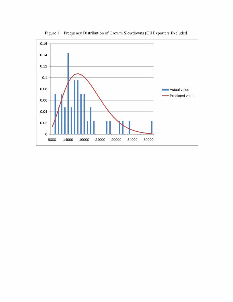
Figure 1. Frequency Distribution of Growth Slowdowns (Oil Exporters Excluded)

0

0.02

0.04

0.06

0.08

0.1

0.12

0.14

0.16

9000 14000 19000 24000 29000 34000 39000

Actual value

Predicted value