what readers are saying - …electronicsengineering.yolasite.com/resources/calculus for the... ·...
TRANSCRIPT
WHAT READERS ARE SAYING
“I wish I had had this book when I needed it most, which was during my pre-med classes.It could have also been a great tool for me in a few medical school courses.”
Dr. Kellie Mosley, Recent Medical School Graduate
“Calculus for the Utterly Confused has proven to be a wonderful review enabling me tomove forward in application of calculus and advanced topics in mathematics. I found iteasy to use and great as a reference for those darker aspects of calculus.”
Aaron Landeville, Engineering Student
“I am so thankful for Calculus for the Utterly Confused! I started out clueless but endedwith an A!”
Erika Dickstein, Business School Student
“As a non-traditional student one thing I have learned is the importance of material sup-plementary to texts. Especially in calculus it helps to have a second source, especiallyone as lucid and fun to read as Calculus for the Utterly Confused. Anyone, whether amath weenie or not, will get something out of this book. With this book, your chances ofsurvival in the calculus jungle are greatly increased.”
Brad Baker, Physics Student

Other books in the Utterly Confused Series include:
Algebra for the Utterly Confused
Astronomy for the Utterly Confused
Beginning French for the Utterly Confused
Beginning Spanish for the Utterly Confused
Chemistry for the Utterly Confused
English Grammar for the Utterly Confused
Financial Aid for the Utterly Confused
Physics for the Utterly Confused
Statistics for the Utterly Confused
Test Taking Strategies and Study Skills for the Utterly Confused
New York Chicago San Francisco Lisbon London MadridMexico City Milan New Delhi San Juan Seoul
Singapore Sydney Toronto
Calculus
for the
Utterly ConfusedSecond Edition
Robert Oman
Daniel Oman
Copyright © 2007 by The McGraw-Hill Companies, Inc. All rights reserved. Manufactured in the United States of America.Except as permitted under the United States Copyright Act of 1976, no part of this publication may be reproduced or dis-tributed in any form or by any means, or stored in a database or retrieval system, without the prior written permission of thepublisher.
0-07-151119-9
The material in this eBook also appears in the print version of this title: 0-07-148158-3.
All trademarks are trademarks of their respective owners. Rather than put a trademark symbol after every occurrence of atrademarked name, we use names in an editorial fashion only, and to the benefit of the trademark owner, with no intentionof infringement of the trademark. Where such designations appear in this book, they have been printed with initial caps.
McGraw-Hill eBooks are available at special quantity discounts to use as premiums and sales promotions, or for use in corporate training programs. For more information, please contact George Hoare, Special Sales, at [email protected] or (212) 904-4069.
TERMS OF USE
This is a copyrighted work and The McGraw-Hill Companies, Inc. (“McGraw-Hill”) and its licensors reserve all rights inand to the work. Use of this work is subject to these terms. Except as permitted under the Copyright Act of 1976 and theright to store and retrieve one copy of the work, you may not decompile, disassemble, reverse engineer, reproduce, modify,create derivative works based upon, transmit, distribute, disseminate, sell, publish or sublicense the work or any part of itwithout McGraw-Hill’s prior consent. You may use the work for your own noncommercial and personal use; any other useof the work is strictly prohibited. Your right to use the work may be terminated if you fail to comply with these terms.
THE WORK IS PROVIDED “AS IS.” McGRAW-HILL AND ITS LICENSORS MAKE NO GUARANTEES OR WAR-RANTIES AS TO THE ACCURACY, ADEQUACY OR COMPLETENESS OF OR RESULTS TO BE OBTAINED FROMUSING THE WORK, INCLUDING ANY INFORMATION THAT CAN BE ACCESSED THROUGH THE WORK VIAHYPERLINK OR OTHERWISE, AND EXPRESSLY DISCLAIM ANY WARRANTY, EXPRESS OR IMPLIED,INCLUDING BUT NOT LIMITED TO IMPLIED WARRANTIES OF MERCHANTABILITY OR FITNESS FOR A PARTICULAR PURPOSE. McGraw-Hill and its licensors do not warrant or guarantee that the functions contained in thework will meet your requirements or that its operation will be uninterrupted or error free. Neither McGraw-Hill nor its licen-sors shall be liable to you or anyone else for any inaccuracy, error or omission, regardless of cause, in the work or for any damages resulting therefrom. McGraw-Hill has no responsibility for the content of any information accessed through thework. Under no circumstances shall McGraw-Hill and/or its licensors be liable for any indirect, incidental, special, punitive,consequential or similar damages that result from the use of or inability to use the work, even if any of them has been advisedof the possibility of such damages. This limitation of liability shall apply to any claim or cause whatsoever whether suchclaim or cause arises in contract, tort or otherwise.
DOI: 10.1036/0071481583

We hope you enjoy thisMcGraw-Hill eBook! If
you’d like more information about this book,its author, or related books and websites,please click here.
Professional
Want to learn more?

To Kelly and Sam
About the Authors
DR ROBERT OMAN received the B.S. degree fromNortheastern University and the Sc.M. and Ph.D.degrees from Brown University, all in physics. Hehas taught mathematics and physics at several col-leges and universities including University ofMinnesota, Northeastern University, University ofSouth Florida, and University of Tampa. He hasalso done research for Litton Industries, UnitedTechnologies, and NASA, where he developed thetheoretical model for the first pressure gauge sentto the moon. He is author of numerous technicalarticles, books, and how-to-study books, tapes, andvideos.
DR DANIEL OMAN received the B.S. degree inphysics from Eckerd College. He received both hisM.S. degree in physics and his Ph.D. in electricalengineering from the University of South Floridawhere he taught many utterly confused students inclasses and one-on-one. He has authored severalbooks and technical articles and has also doneresearch on CO2 lasers and solar cells. Dan hasspent ten years in the semiconductor manufactur-ing industry with AT&T Bell Labs, LucentTechnologies, and Agere Systems.
Copyright © 2007 by The McGraw-Hill Companies, Inc. Click here for terms of use.
vii
Contents
A Special Message xi
How to Study Calculus xiii
Preface xv
Chapter 1 Mathematical Background 1
1-1 Solving Equations 2
1-2 Binomial Expansions 4
1-3 Trigonometry 5
1-4 Coordinate Systems 6
1-5 Logarithms and Exponents 8
1-6 Functions and Graphs 10
1-7 Conics 16
1-8 Graphing Trigonometric Functions 23
Test Yourself 27
Answers 28
Chapter 2 Limits and Continuity 31
Test Yourself 37
Answers 38
For more information about this title, click here
Chapter 3 Derivatives 41
3-1 Polynomials 43
3-2 Product and Quotient Rule 48
3-3 Trigonometric Functions 49
3-4 Implicit Differentiation 50
3-5 Change of Variable 52
3-6 Chain Rule 53
3-7 Logarithms and Exponents 55
3-8 L’Hopital’s Rule 56
Test Yourself 58
Answers 58
Chapter 4 Graphing 61
Guidelines for Graphing with Calculus 72
Test Yourself 77
Answers 77
Chapter 5 Max-Min Problems 81
Guidelines for Max-Min Problems 84
Test Yourself 90
Answers 91
Chapter 6 Related Rate Problems 95
Test Yourself 108
Answers 109
Chapter 7 Integration 113
7-1 The Antiderivative 114
7-2 Area Under the Curve 123
7-3 Average Value of a Function 135
7-4 Area between Curves Using dy 139
Test Yourself 143
Answers 143
viii CONTENTS
Chapter 8 Trigonometric Functions 147
8-1 Right Angle Trigonometry 148
8-2 Special Triangles 152
8-3 Radians and Small Angles 154
8-4 Non-Right Angle Trigonometry 156
8-5 Trigonometric Functions 160
8-6 Identities 162
8-7 Differentiating Trigonometric Functions 166
8-8 Integrating Trigonometric Functions 170
Test Yourself 175
Answers 176
Chapter 9 Exponents and Logarithms 179
9-1 Exponent Basics 180
9-2 Exponential Functions 181
9-3 The Number e 186
9-4 Logarithms 191
9-5 Growth and Decay Problems 195
9-6 The Natural Logarithm 202
9-7 Limited Exponential Growth 203
9-8 The Logistic Function 212
Test Yourself 215
Answers 216
Chapter 10 More Integrals 221
10-1 Volumes 222
10-2 Arc Lengths 226
10-3 Surfaces of Revolution 228
10-4 Techniques of Integration 229
10-5 Integration by Parts 236
10-6 Partial Fractions 238
Contents ix
10-7 Integrals from Tables 242
10-8 Approximate Methods 243
Test Yourself 249
Answers 249
Mathematical Tables 253
Index 259
x CONTENTS
xi
A Special Message tothe Utterly ConfusedCalculus Student
Our message to the utterly confused calculus student is very simple: You don’thave to be confused anymore.
We were once confused calculus students. We aren’t confused anymore. Wehave taught many utterly confused calculus students both in formal class set-tings and one-on-one. All this experience has taught us what causes confusionin calculus and how to eliminate that confusion. The topics we discuss here areaimed right at the heart of those topics that we know cause the most trouble.Follow us through this book, and you won’t be confused anymore either.
Anyone who has taught calculus will tell you that there are two problem areasthat prevent students from learning the subject. The first problem is a lack ofalgebra skills or perhaps a lack of confidence in applying recently learnedalgebra skills. We attack this problem two ways. One of the largest chapters inthis book is the one devoted to a review of the algebra skills you need to besuccessful in working calculus problems. Don’t pass by this chapter. There areinsights for even those who consider themselves good at algebra. When we doa problem we take you through the steps, the calculus steps and all those pesky
Copyright © 2007 by The McGraw-Hill Companies, Inc. Click here for terms of use.
little algebra steps, tricks some might call them. When we give an example it isa complete presentation. Not only do we do the problem completely but alsowe explain along the way why things are done a certain way.
The second problem of the utterly confused calculus student is the inability toset up the problems. In most problems the calculus is easy, the algebra possiblytedious, but writing the problem in mathematical statements the most difficultstep of all. Translating a word problem into a math problem (words to equa-tion) is not easy. We spend time in the problems showing you how to make wordsentences into mathematical equations. Where there are patterns to problemswe point them out so when you see similar problems, on tests perhaps, you willremember how to do them.
Our message to utterly confused calculus students is simple. You don’t have tobe confused anymore. We have been there, done that, know what it takes toremove the confusion, and have written it all down for you.
xii A SPECIAL MESSAGE
xiii
How to Study Calculus
Calculus courses are different from most courses in other disciplines. One bigdifference is in testing. There is very little writing in a calculus test. There is alot of mathematical manipulation.
In many disciplines you learn the material by reading and listening and demon-strate mastery of that material by writing about it. In mathematics there is somereading, and some listening, but demonstrating mastery of the material is bydoing problems.
For example there is a great deal of reading in a history course, but mastery ofthe material is demonstrated by writing about history. In your calculus coursethere should be a lot of problem solving with mastery of the material demon-strated by doing problems.
In your calculus course, practicing working potential problems is essential tosuccess on the tests. Practicing problems, not just reading them but actuallywriting them down, may be the only way for you to achieve the most modest ofsuccess on a calculus test.
To succeed on your calculus tests you need to do three things, PROBLEMS,PROBLEMS, and PROBLEMS. Practice doing problems typical of what youexpect on the exam and you will do well on that exam. This book containsexplanations of how to do many problems that we have found to be the mostconfusing to our students. Understanding these problems will help you tounderstand calculus and do well on the exams.
Copyright © 2007 by The McGraw-Hill Companies, Inc. Click here for terms of use.
General Guidelines for Effective
Calculus Study
1. If at all possible avoid last minute cramming. It is inefficient.
2. Concentrate your time on your best estimate of those problems that aregoing to be on the tests.
3. Review your lecture notes regularly, not just before the test.
4. Keep up. Do the homework regularly. Watching your instructor do a prob-lem that you have not even attempted is not efficient.
5. Taking a course is not a spectator event. Try the problems, get confused if that’swhat it takes, but don’t expect to absorb calculus. What you absorb doesn’t mat-ter on the test. It is what comes off the end of your pencil that counts.
6. Consider starting an informal study group. Pick people to study with whostudy and don’t whine. When you study with someone agree to stick to thetopic and help one other.
Preparing for Tests
1. Expect problems similar to the ones done in class. Practice doing them.Don’t just read the solutions.
2. Look for modifications of problems discussed in class.
3. If old tests are available, work the problems.
4. Make sure there are no little mathematical “tricks” that will cause you prob-lems on the test.
Test Taking Strategies
1. Avoid prolonged contact with fellow students just before the test. The nerv-ous tension, frustration, and defeatism expressed by fellow students are notfor you.
2. Decide whether to do the problems in order or look over the entire test anddo the easiest first. This is a personal preference. Do what works best for you.
3. Know where you are timewise during the test.
4. Do the problems as neatly as you can.
5. Ask yourself if an answer is reasonable. If a return on investment answer is0.03%, it is probably wrong.
xiv HOW TO STUDY CALCULUS
Preface
The purpose of this book is to present basic calculus concepts and show youhow to do the problems. The emphasis is on problems with the concepts devel-oped within the context of the problems. In this way the development of thecalculus comes about as a means of solving problems. Another advantage ofthis approach is that performance in a calculus course is measured by yourability to do problems. We emphasize problems.
This book is intended as a supplement in your formal study and application ofcalculus. It is not intended to be a complete coverage of all the topics you mayencounter in your calculus course. We have identified those topics that causethe most confusion among students and have concentrated on those topics.Skill development in translating words to equations and attention to algebraicmanipulation are emphasized.
This book is intended for the nonengineering calculus student. Those studyingcalculus for scientists and engineers may also benefit from this book Conceptsare discussed but the main thrust of the book is to show you how to solve appliedproblems. We have used problems from business, medicine, finance, economics,chemistry, sociology, physics, and health and environmental sciences. All theproblems are at a level understandable to those in different disciplines.
This book should also serve as a reference to those already working in the var-ious disciplines where calculus is employed. If you encounter calculus occa-sionally and need a simple reference that will explain how problems are donethis book should be a help to you.
xvCopyright © 2007 by The McGraw-Hill Companies, Inc. Click here for terms of use.
It is the sincere desire of the authors that this book help you to better understandcalculus concepts and be able to work the associated problems. We would like tothank the many students who have contributed to this work, many of whomstarted out utterly confused, by offering suggestions for improvements. Also wewould like to thank the people at McGraw-Hill who have confidence in ourapproach to teaching calculus and support this second edition.
Robert M. OmanSt. Petersburg, Florida
Daniel M. OmanSingapore
xvi PREFACE
Calculus
for the
Utterly Confused

This page intentionally left blank
CHAPTER 1
MATHEMATICALBACKGROUND
You should read this chapter if you need to review or you need to learn about
Methods of solving quadratic equations
The binomial expansion
Trigonometric functions––right angle trig and graphs
The various coordinate systems
Basics of logarithms and exponents
Graphing algebraic and trigonometric functions
1
Copyright © 2007 by The McGraw-Hill Companies, Inc. Click here for terms of use.
Some of the topics may be familiar to you, while others may not. Depending onthe mathematical level of your course and your mathematical background,some topics may not be of interest to you.
Each topic is covered in sufficient depth to allow you to perform the mathe-matical manipulations necessary for a particular problem without gettingbogged down in lengthy derivations. The explanations are, of necessity, brief. Ifyou are totally unfamiliar with a topic it may be necessary for you to consult analgebra or calculus text for a more thorough explanation.
The most efficient use of this chapter is for you to do a brief review of the top-ics, spending time on those sections that are unfamiliar to you and that you knowyou will need in your course, and then refer to specific topics as they are encoun-tered in the solution to problems. Even if you are familiar with a topic reviewmight “fill in the gaps” or give you a better insight into certain mathematicaloperations. With this reference you should be able to perform all the algebraicoperations necessary to complete the problems in your calculus course.
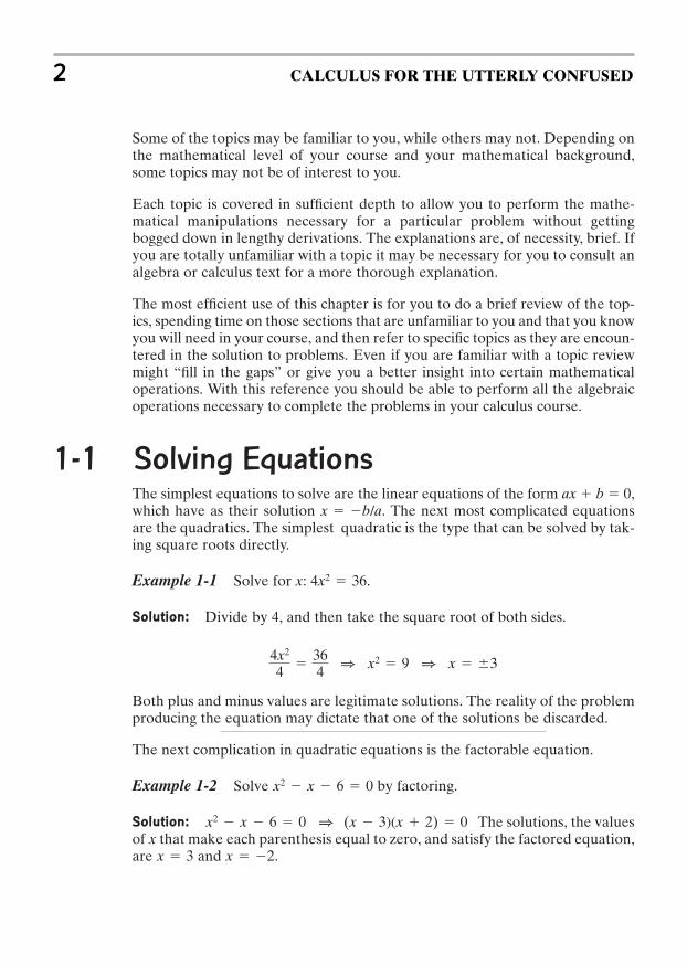
1-1 Solving EquationsThe simplest equations to solve are the linear equations of the form ax b 0,which have as their solution . The next most complicated equationsare the quadratics. The simplest quadratic is the type that can be solved by tak-ing square roots directly.
Example 1-1 Solve for x: .
Solution: Divide by 4, and then take the square root of both sides.
Both plus and minus values are legitimate solutions. The reality of the problemproducing the equation may dictate that one of the solutions be discarded.
The next complication in quadratic equations is the factorable equation.
Example 1-2 Solve by factoring.
Solution: The solutions, the valuesof that make each parenthesis equal to zero, and satisfy the factored equation,are and .x 2x 3
x(x 3)(x 2) 01x2 x 6 0
x2 x 6 0
4x2
4 364 1 x2 9 1 x 3
4x2 36
x b/a
2 CALCULUS FOR THE UTTERLY CONFUSED
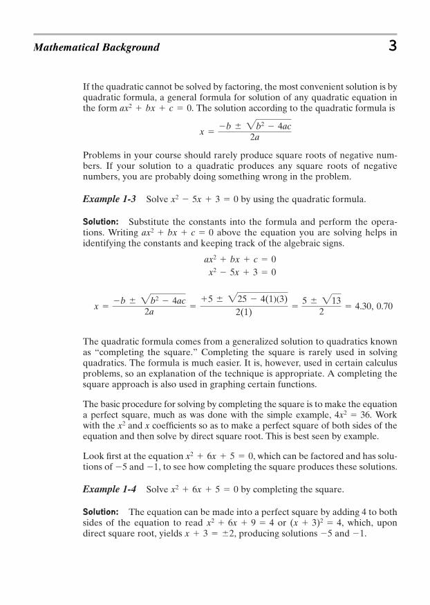
If the quadratic cannot be solved by factoring, the most convenient solution is byquadratic formula, a general formula for solution of any quadratic equation inthe form . The solution according to the quadratic formula is
Problems in your course should rarely produce square roots of negative num-bers. If your solution to a quadratic produces any square roots of negativenumbers, you are probably doing something wrong in the problem.
Example 1-3 Solve by using the quadratic formula.
Solution: Substitute the constants into the formula and perform the opera-tions. Writing above the equation you are solving helps inidentifying the constants and keeping track of the algebraic signs.
The quadratic formula comes from a generalized solution to quadratics knownas “completing the square.” Completing the square is rarely used in solvingquadratics. The formula is much easier. It is, however, used in certain calculusproblems, so an explanation of the technique is appropriate. A completing thesquare approach is also used in graphing certain functions.
The basic procedure for solving by completing the square is to make the equationa perfect square, much as was done with the simple example, . Workwith the and x coefficients so as to make a perfect square of both sides of theequation and then solve by direct square root. This is best seen by example.
Look first at the equation , which can be factored and has solu-tions of 5 and 1, to see how completing the square produces these solutions.
Example 1-4 Solve by completing the square.
Solution: The equation can be made into a perfect square by adding 4 to bothsides of the equation to read or , which, upondirect square root, yields , producing solutions 5 and 1.x 3 2
(x 3)2 4x2 6x 9 4
x2 6x 5 0
x2 6x 5 0
x24x2 36
x b 2b2 4ac
2a
5 225 4(1)(3)2(1)
5 213
2 4.30, 0.70
ax2 bx c 0x2 5x 3 0
ax2 bx c 0
x2 5x 3 0
x b 2b2 4ac
2a
ax2 bx c 0
Mathematical Background 3

As you can imagine the right combina-tion of coefficients of and x can makethe problem awkward. Most calculusproblems involving completing thesquare are not especially difficult. Thegeneral procedure for completing thesquare is the following:
• If necessary, divide to make the coef-ficient of the term equal to 1.
• Move the constant term to the rightside of the equation.
• Take 1/2 of the x coefficient, square it,and add to both sides of the equation.This makes the left side a perfectsquare and the right side a number.
• Write the left side as a perfect squareand take the square root of both sidesfor the solution.
Example 1-5 Solve by completing the square.
Solution: Move the 1, the constant term, to the right side: . Add1/2 of 4 (the coefficient of x) squared to both sides: x2 4x 4 4 1. Theleft side is a perfect square and the right side a number: . Takesquare roots for the solutions: or .
Certain cubic equations such as can be solved directly producing the sin-gle answer . Cubic equations with quadratic ( ) and linear (x) terms canbe solved by factoring (if possible) or approximated using graphical techniques.Calculus will allow you to apply graphical techniques to solving cubics.
1-2 Binomial ExpansionsSquaring is done so often that most would immediately write
. Cubing is not so familiar but easily accomplished bymultiplying by to obtain .
There is a simple procedure for finding the power of . Envision astring of s multiplied together . Notice that the first term hascoefficient 1 with a raised to the power, and the last term has coefficient1 with b raised to the power. The terms in between contain a to progressivelynth
nth(a b)n(a b)
(a b)nth
a3 3a2b 3ab2 b3(a b)(a2 2ab b2)(a b)a2 2ab b2
(a b)
x2x 2x3 8
x 2 23, 2 23x 2 23(x 2)2 3
x2 4x 1
x2 4x 1 0
x2
x2
4 CALCULUS FOR THE UTTERLY CONFUSED
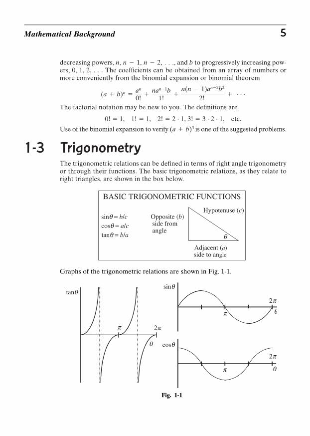
decreasing powers, , and b to progressively increasing pow-ers, 0, 1, 2, . . . The coefficients can be obtained from an array of numbers ormore conveniently from the binomial expansion or binomial theorem
The factorial notation may be new to you. The definitions are
0! 1, 1! 1, 2! 2 ⋅ 1, 3! 3 ⋅ 2 ⋅ 1, etc.
Use of the binomial expansion to verify is one of the suggested problems.
1-3 TrigonometryThe trigonometric relations can be defined in terms of right angle trigonometryor through their functions. The basic trigonometric relations, as they relate toright triangles, are shown in the box below.
(a b)3
(a b)n an
0!
nan1b1!
n(n 1)an2b2
2! c
n, n 1, n 2, . . .
Mathematical Background 5
Graphs of the trigonometric relations are shown in Fig. 1-1.
Fig. 1-1
tanq = b/acosq = a/csinq = b/c Opposite (b)
side fromangle
Adjacent (a)side to angle
Hypotenuse (c)
BASIC TRIGONOMETRIC FUNCTIONS
q
2p
2p
2p
tanqsinq
cosq
p
p
p
q
q
q
6 CALCULUS FOR THE UTTERLY CONFUSED
The tangent function is also defined in terms of sine and cosine:.
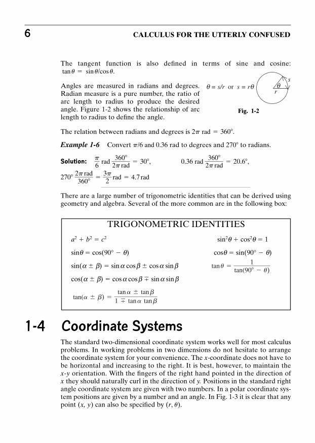
Angles are measured in radians and degrees.Radian measure is a pure number, the ratio ofarc length to radius to produce the desiredangle. Figure 1-2 shows the relationship of arclength to radius to define the angle.
The relation between radians and degrees is .
Example 1-6 Convert rad to degrees and 270 to radians.
Solution: , ,
There are a large number of trigonometric identities that can be derived usinggeometry and algebra. Several of the more common are in the following box:
2702p rad360
3p2 rad 4.7 rad
0.36 rad360
2p rad 20.6
p
6rad
3602p rad
30
p/6 and 0.36
2p rad 360
tan u sin u/cos u
1-4 Coordinate SystemsThe standard two-dimensional coordinate system works well for most calculusproblems. In working problems in two dimensions do not hesitate to arrangethe coordinate system for your convenience. The x-coordinate does not have tobe horizontal and increasing to the right. It is best, however, to maintain thex-y orientation. With the fingers of the right hand pointed in the direction ofx they should naturally curl in the direction of y. Positions in the standard rightangle coordinate system are given with two numbers. In a polar coordinate sys-tem positions are given by a number and an angle. In Fig. 1-3 it is clear that anypoint (x, y) can also be specified by ( ). r, u
Fig. 1-2
TRIGONOMETRIC IDENTITIES
a2 b2 c2 sin2q cos2q 1
sinq cos(90° q) cosq sin(90° q)
sin(a b) sin a cos b cos a sin b
cos(a b) cos a cos b sin a sin b
tan(a b) tana tanb
1 7 tana tanb
tanu 1
tan(90 u)
s
rq = s/r or s = rq q
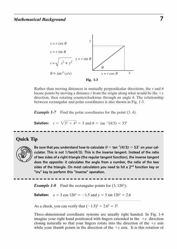
Rather than moving distances in mutually perpendicular directions, the r andlocate points by moving a distance r from the origin along what would be the xdirection, then rotating counterclockwise through an angle . The relationshipbetween rectangular and polar coordinates is also shown in Fig. 1-3.
Example 1-7 Find the polar coordinates for the point (3, 4).
Solution: and u tan 1(4/3) 53r 232 42 5
u
u
Mathematical Background 7
Example 1-8 Find the rectangular points for (3, 120°).
Solution: x 3 cos 120° 1.5 and y 3 sin 120° 2.6
As a check, you can verify that (1.5)2 2.62 32.
Three-dimensional coordinate systems are usually right handed. In Fig. 1-4imagine your right hand positioned with fingers extended in the x directionclosing naturally so that your fingers rotate into the direction of the y axiswhile your thumb points in the direction of the z axis. It is this rotation of
Fig. 1-3
Quick Tip
Be sure that you understand how to calculate q tan−1(4/3) 53 on your cal-
culator. This is not 1/tan(4/3). This is the inverse tangent. Instead of the ratio
of two sides of a right triangle (the regular tangent function), the inverse tangent
does the opposite: it calculates the angle from a number, the ratio of the two
sides of the triangle. On most calculators you need to hit a 2nd function key or
”inv” key to perform this ”inverse” operation.
x
y
q = tan–1 (y/x)
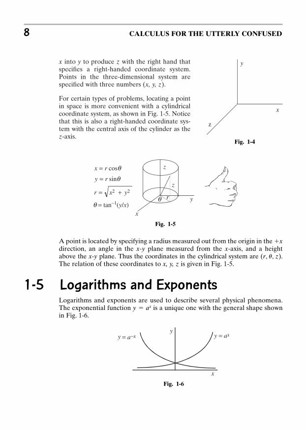
x = r cos q
y = r sin q
x2 + y2r =y = r sin q
x = r cos qq
x into y to produce z with the right hand thatspecifies a right-handed coordinate system.Points in the three-dimensional system arespecified with three numbers (x, y, z).
For certain types of problems, locating a pointin space is more convenient with a cylindricalcoordinate system, as shown in Fig. 1-5. Noticethat this is also a right-handed coordinate sys-tem with the central axis of the cylinder as thez-axis.
8 CALCULUS FOR THE UTTERLY CONFUSED
A point is located by specifying a radius measured out from the origin in the xdirection, an angle in the x-y plane measured from the x-axis, and a heightabove the x-y plane. Thus the coordinates in the cylindrical system are .The relation of these coordinates to x, y, z is given in Fig. 1-5.
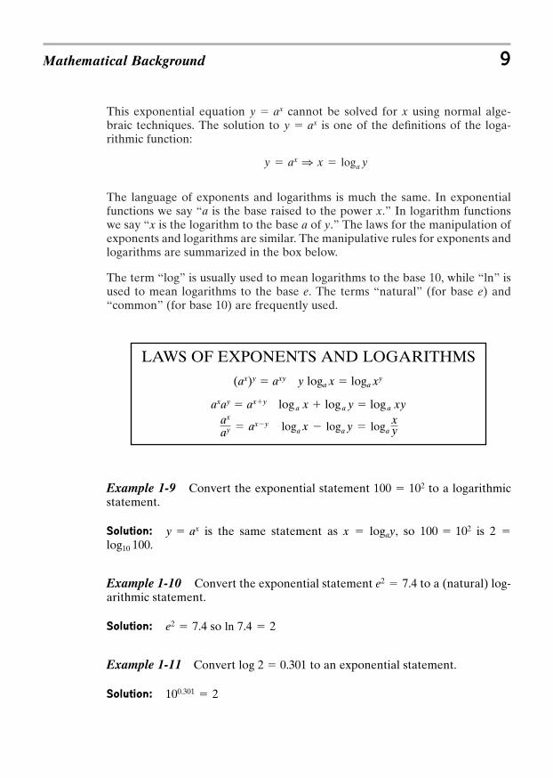
1-5 Logarithms and ExponentsLogarithms and exponents are used to describe several physical phenomena.The exponential function is a unique one with the general shape shownin Fig. 1-6.
y ax
(r, u, z)
Fig. 1-5
Fig. 1-6
x
z
y
Fig. 1-4
x
y
z
z
rq = tan−1(y/x)
sinqcosq
y2x2r
ry
rx
+=
==
q
x
yy = axy = a-x
This exponential equation cannot be solved for x using normal alge-braic techniques. The solution to is one of the definitions of the loga-rithmic function:
The language of exponents and logarithms is much the same. In exponentialfunctions we say “a is the base raised to the power x.” In logarithm functionswe say “x is the logarithm to the base a of y.” The laws for the manipulation ofexponents and logarithms are similar. The manipulative rules for exponents andlogarithms are summarized in the box below.
The term “log” is usually used to mean logarithms to the base 10, while “ln” isused to mean logarithms to the base e. The terms “natural” (for base e) and“common” (for base 10) are frequently used.
y ax 1 x loga y
y axy ax
Mathematical Background 9
Example 1-9 Convert the exponential statement to a logarithmicstatement.
Solution: is the same statement as x logay, so is 2 log10 100.
Example 1-10 Convert the exponential statement to a (natural) log-arithmic statement.
Solution: so
Example 1-11 Convert log 2 0.301 to an exponential statement.
Solution: 100.301 2
ln 7.4 2e2 7.4
e2 7.4
100 102y ax
100 102
LAWS OF EXPONENTS AND LOGARITHMS
(ax)y axy y loga x loga xy
axay axy log a x log a y log a xy
loga x loga y logaxy
ax
ay axy

Example 1-12 Find log(2.1)(4.3)1.6.
Solution: On your hand calculator raise 4.3 to the 1.6 power and multiply thisresult by 2.1. Now take the log to obtain 1.34.
Second Solution: Applying the laws for the manipulation of logarithms write:
log(2.1)(4.3)1.6 log 2.1 log 4.31.6 log 2.1 1.6 log 4.3 0.32 1.01 1.33
(Note the round-off error in this second solution.) This second solution is rarelyused for numbers. It is, however, used in solving equations.
Example 1-13 Solve .
Solution: Apply a manipulative rule for logarithms: or.
Now switch to exponentials: x e3.31 27.4
3.31 ln x4 ln 2 ln x
4 ln 2x
10 CALCULUS FOR THE UTTERLY CONFUSED
Quick Tip
A very convenient phrase to remember in working with logarithms is “a logarithm
is an exponent.” If the logarithm of something is a number or an expression, then
that number or expression is the exponent of the base of the logarithm.
1-6 Functions and GraphsFunctions can be viewed as a series of mathematical orders. The typical func-tion is written starting with y, or , read as “f of x,” short for function of x.The mathematical function is a series of orders oroperations to be performed on an as yet to be specified value of x. This set oforders is: square x, add 2 times x, and add 1. The operations specified in thefunction can be performed on individual values of x or graphed to show a con-tinuous “function.” It is the graphing that is most encountered in calculus. We’lllook at a variety of algebraic functions eventually leading into the concept ofthe limit.
y or f(x) x2 2x 1f(x)
Example 1-14 Perform the functions on the number 2 orfind .
Solution: Performing the operations on the specified function
In visualizing problems it is very helpful to know what certain functions looklike. You should review the functions described in this section until you canlook at a function and picture “in your mind’s eye” what it looks like. This skillwill prove valuable to you as you progress through your calculus course.
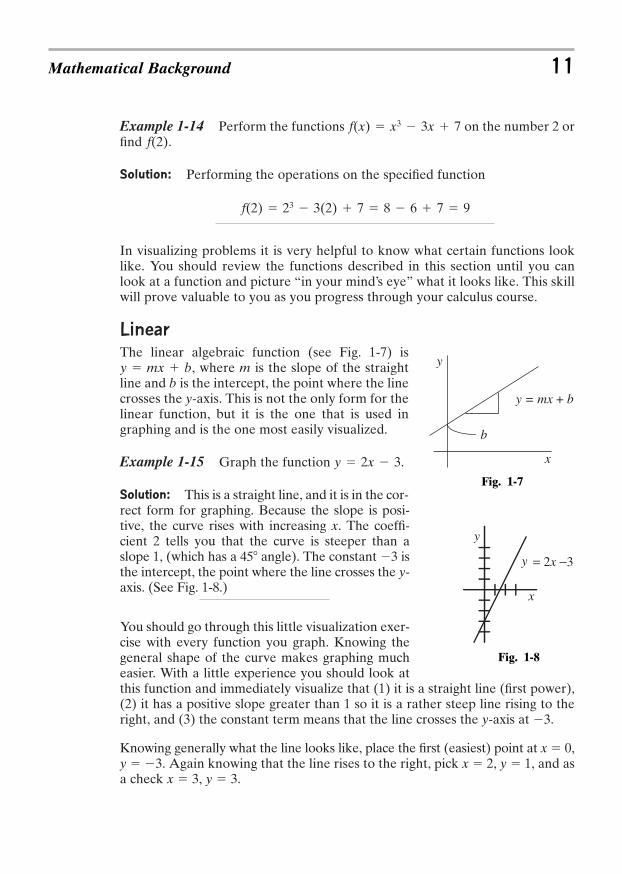
Linear
The linear algebraic function (see Fig. 1-7) is, where m is the slope of the straight
line and b is the intercept, the point where the linecrosses the y-axis. This is not the only form for thelinear function, but it is the one that is used ingraphing and is the one most easily visualized.
Example 1-15 Graph the function .
Solution: This is a straight line, and it is in the cor-rect form for graphing. Because the slope is posi-tive, the curve rises with increasing x. The coeffi-cient 2 tells you that the curve is steeper than aslope 1, (which has a 45 angle). The constant 3 isthe intercept, the point where the line crosses the y-axis. (See Fig. 1-8.)
You should go through this little visualization exer-cise with every function you graph. Knowing thegeneral shape of the curve makes graphing mucheasier. With a little experience you should look atthis function and immediately visualize that (1) it is a straight line (first power),(2) it has a positive slope greater than 1 so it is a rather steep line rising to theright, and (3) the constant term means that the line crosses the y-axis at 3.
Knowing generally what the line looks like, place the first (easiest) point at x 0,y 3. Again knowing that the line rises to the right, pick x 2, y 1, and asa check x 3, y 3.
y 2x 3
y mx b
f(2) 23 3(2) 7 8 6 7 9
f(2)f(x) x3 3x 7
Mathematical Background 11
Fig. 1-7
Fig. 1-8
y
x
b
y = mx + b
x
y
y = 2x −3
If you are not familiar with visualizing the function before you start calculatingpoints, graph a few straight lines, but go through the exercise outlined abovebefore you place any points on the graph.
Quadratics
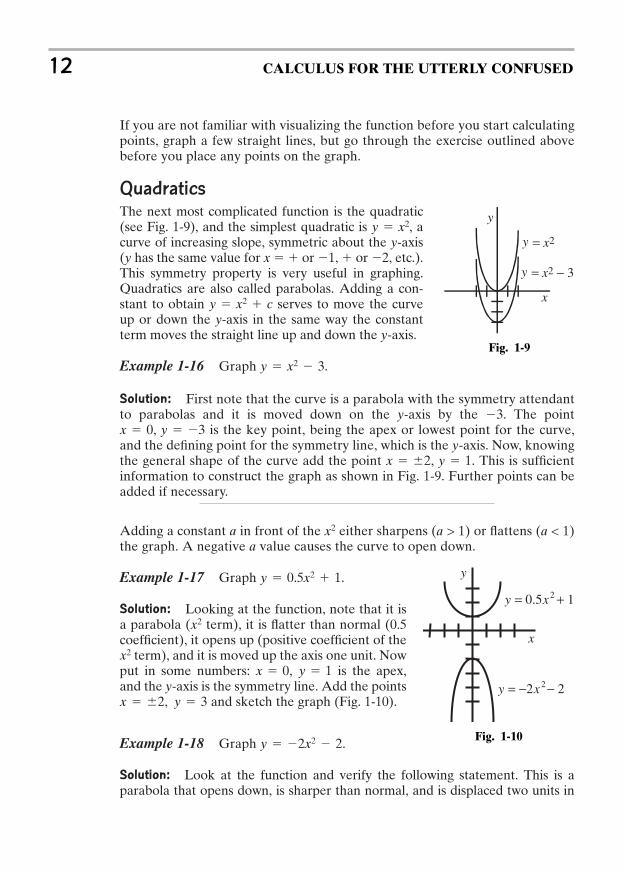
The next most complicated function is the quadratic(see Fig. 1-9), and the simplest quadratic is , acurve of increasing slope, symmetric about the y-axis(y has the same value for x or 1, or 2, etc.).This symmetry property is very useful in graphing.Quadratics are also called parabolas. Adding a con-stant to obtain serves to move the curveup or down the y-axis in the same way the constantterm moves the straight line up and down the y-axis.
Example 1-16 Graph .
Solution: First note that the curve is a parabola with the symmetry attendantto parabolas and it is moved down on the y-axis by the 3. The point
is the key point, being the apex or lowest point for the curve,and the defining point for the symmetry line, which is the y-axis. Now, knowingthe general shape of the curve add the point . This is sufficientinformation to construct the graph as shown in Fig. 1-9. Further points can beadded if necessary.
Adding a constant a in front of the x2 either sharpens (a > 1) or flattens (a < 1)the graph. A negative a value causes the curve to open down.
Example 1-17 Graph .
Solution: Looking at the function, note that it isa parabola ( term), it is flatter than normal (0.5coefficient), it opens up (positive coefficient of the
term), and it is moved up the axis one unit. Nowput in some numbers: is the apex,and the y-axis is the symmetry line. Add the points
and sketch the graph (Fig. 1-10).
Example 1-18 Graph .
Solution: Look at the function and verify the following statement. This is aparabola that opens down, is sharper than normal, and is displaced two units in
y 2x2 2
x 2, y 3
x 0, y 1x2
x2
y 0.5x2 1
x 2, y 1
x 0, y 3
y x2 3
y x2 c
y x2
12 CALCULUS FOR THE UTTERLY CONFUSED
Fig. 1-9
x
y
y = x2
y = x2 − 3
Fig. 1-10
x
− 22 2−= xy
5.0 2 + 1= xy
y
the negative direction. Put in the two points and and verify thegraph shown in Fig. 1-10.
Adding a linear term, a constant times x, so that the function has the formproduces the most complicated quadratic. The addition of
this constant term moves the curve both up and down and sideways. If thequadratic function is factorable then the places where it crosses the x-axis areobtained directly from the factored form.
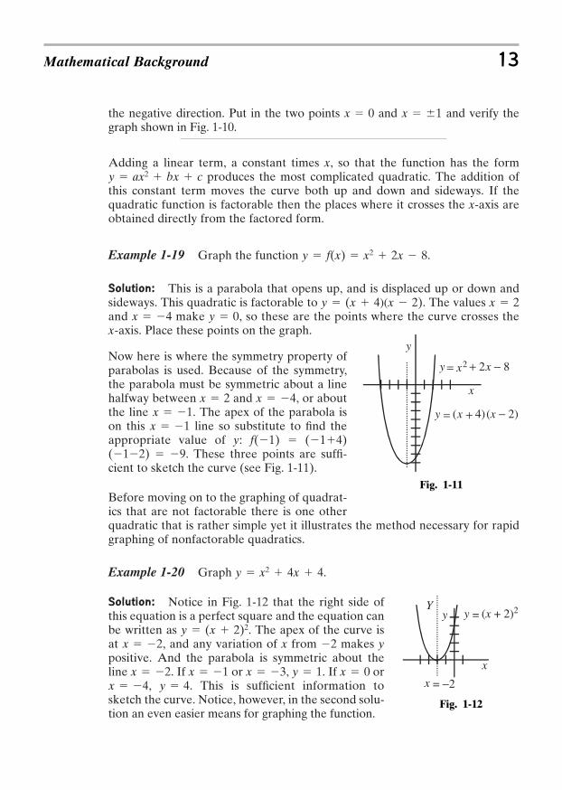
Example 1-19 Graph the function .
Solution: This is a parabola that opens up, and is displaced up or down andsideways. This quadratic is factorable to . The values and make , so these are the points where the curve crosses thex-axis. Place these points on the graph.
Now here is where the symmetry property ofparabolas is used. Because of the symmetry,the parabola must be symmetric about a linehalfway between and , or aboutthe line . The apex of the parabola ison this line so substitute to find theappropriate value of y: f(1) (14)(12) 9. These three points are suffi-cient to sketch the curve (see Fig. 1-11).
Before moving on to the graphing of quadrat-ics that are not factorable there is one otherquadratic that is rather simple yet it illustrates the method necessary for rapidgraphing of nonfactorable quadratics.
Example 1-20 Graph .
Solution: Notice in Fig. 1-12 that the right side ofthis equation is a perfect square and the equation canbe written as . The apex of the curve isat , and any variation of x from 2 makes ypositive. And the parabola is symmetric about theline . If or , . If or
, . This is sufficient information tosketch the curve. Notice, however, in the second solu-tion an even easier means for graphing the function.
y 4x 4x 0y 1x 3x 1x 2
x 2y (x 2)2
y x2 4x 4
x 1x 1
x 4x 2
y 0x 4x 2y (x 4)(x 2)
y f(x) x2 2x 8
y ax2 bx c
x 1x 0
Mathematical Background 13
Fig. 1-12
Fig. 1-11
x
y
y x= x2 + 2 − 8
y x= +( (x − 2)4)
y = (x + 2)2
x
yY
x = −2
Second Solution: The curve can be written in the form if is definedas . At , and the line effectively defines a newaxis. Call it the Y-axis. This is the axis of symmetry determined in the previoussolution. Drawing in the new axis allows graphing of the simple equation
about this new axis.y X 2
x 2X 0x 2X x 2Xy X 2
14 CALCULUS FOR THE UTTERLY CONFUSED
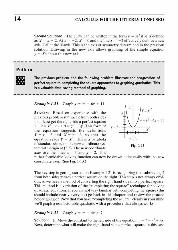
Example 1-21 Graph .
Solution: Based on experience with theprevious problem subtract 2 from both sidesto at least get the right side a perfect square:y 2 x2 6x 9 (x 3)2. This form ofthe equation suggests the definitions
and , so that theequation reads . This is a parabolaof standard shape on the new coordinate sys-tem with origin at . The new coordinateaxes are the lines and . Thisrather formidable looking function can now be drawn quite easily with the newcoordinate axes. (See Fig. 1-13.)
The key step in getting started on Example 1-21 is recognizing that subtracting 2from both sides makes a perfect square on the right. This step is not always obvi-ous, so we need a method of converting the right-hand side into a perfect square.This method is a variation of the “completing the square” technique for solvingquadratic equations. If you are not very familiar with completing the square (thisshould include nearly everyone) go back in this chapter and review the processbefore going on. Now that you have “completing the square” clearly in your mindwe’ll graph a nonfactorable quadratic with a procedure that always works.
Example 1-22 Graph .
Solution: 1. Move the constant to the left side of the equation: y 7 x2 4x.Next, determine what will make the right-hand side a perfect square. In this case
y x2 4x 7
y 2x 3(3,2)
Y X 2X x 3Y y 2
y x2 6x 11
Pattern
The previous problem and the following problem illustrate the progression of
perfect square to completing the square approaches to graphing quadratics. This
is a valuable time-saving method of graphing.
Fig. 1-13
x
y
X
Y
y = x - 6x + 112
Y = X 2
y = 2
x = 3

4 makes a perfect square on the right so addthis to both sides: or
.
2. Now, make the shift in axes with the defi-nitions and . The originof the “new” coordinate axes is (2,3).Determining the origin from these definingequations helps to prevent scrambling the(2,3) and getting the origin in the wrongplace. The values (2,3) make X and Y zeroand this is the apex of the curve on thenew coordinate axes.
3. Graph the curve as shown in Fig. 1-14.
Higher Power Curves
The graphing of cubic and higher power curvesrequires techniques you will learn in your calculuscourse. There are, however, some features of higherpower curves that can be learned from an “algebraic”look at the curves.
The simple curves for and are shownin Fig. 1-15. Adding a constant term to either of thesecurves serves to move them up or down on the y-axisthe same as it does for a quadratic or straight line.Cubics plus a constant are relatively easy to sketch.Adding a quadratic or linear term adds complicationsthat are almost always easiest handled by learning thecalculus necessary to help you graph the curve. If acurve contains an term, this term will eventuallypredominate for sufficiently large x.
Operationally, this means that if you have an expressiony x3 ()x2 ()x (), while there may be consider-able gyration of the curve near the origin, for large (pos-itive or negative) x the curve will eventually take the shape shown in Fig. 1-15.
The same is true for other higher power curves. The curve is similar inshape to , it just rises more rapidly. The addition of other (lower than 4)power terms again may add some interesting twists to the curve but for large xit will eventually rise sharply.
y x2y x4
x3
y x3y x3
Y X 2
X x 2Y y 3
y 3 (x 2)2y 3 x2 4x 4
Mathematical Background 15
Fig. 1-15
Fig. 1-14
x
y
X
Y
y x x= + +2 4
x = −2
y = 3
7
y = −x3 y = x3
x
y
1-7 ConicsThe next general category of curves is called conics, because they have shapesgenerated by passing a plane through a cone. They contain x and y terms to thesecond power. The simplest of these curves is generated with and equal toa constant. More complicated curves have positive coefficients for these terms,and the most complicated conics have positive and negative coefficients.
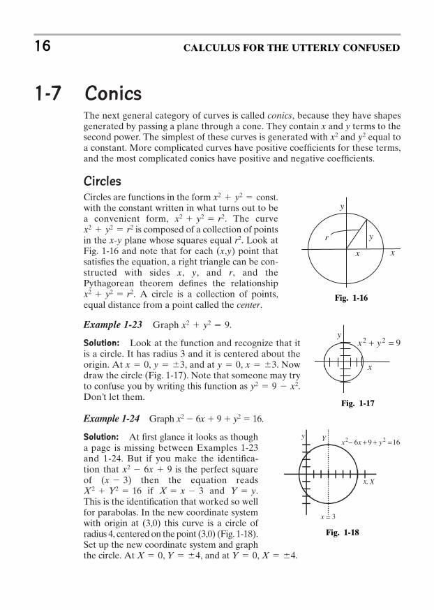
Circles
Circles are functions in the form with the constant written in what turns out to bea convenient form, . The curve
is composed of a collection of pointsin the x-y plane whose squares equal . Look atFig. 1-16 and note that for each point thatsatisfies the equation, a right triangle can be con-structed with sides x, y, and r, and thePythagorean theorem defines the relationship
. A circle is a collection of points,equal distance from a point called the center.
Example 1-23 Graph .
Solution: Look at the function and recognize that itis a circle. It has radius 3 and it is centered about theorigin. At , , and at . Nowdraw the circle (Fig. 1-17). Note that someone may tryto confuse you by writing this function as .Don’t let them.
Example 1-24 Graph x2 6x 9 y2 16.
Solution: At first glance it looks as thougha page is missing between Examples 1-23and 1-24. But if you make the identifica-tion that is the perfect squareof then the equation reads
if and .This is the identification that worked so wellfor parabolas. In the new coordinate systemwith origin at (3,0) this curve is a circle ofradius 4, centered on the point (3,0) (Fig. 1-18).Set up the new coordinate system and graphthe circle. At , , and at , .X 4Y 0Y 4X 0
Y yX x 3X 2 Y2 16(x 3)
x2 6x 9
y2 9 x2
x 3y 0,y 3x 0
x2 y2 9
x2 y2 r2
(x,y)r2
x2 y2 r2x2 y2 r2
x2 y2 const.
y2x2
16 CALCULUS FOR THE UTTERLY CONFUSED
Fig. 1-16
y
xx
yr
Fig. 1-17
922 =+ yxy
x
x, X
y Y
x = 3
169− 6 22 =++ yxx
Fig. 1-18
If the function were written it would not have been quite soeasy to recognize the curve. Looking at this latter rearrangement, the clue thatthis is a circle is that the and terms are both positive when they are togetheron the same side of the equation. No matter how scrambled the terms are, if youcan recognize that the curve is a circle you can separate out the terms and makesome sense out of them by making perfect squares. This next problem will giveyou an example that is about as complicated as you will encounter.
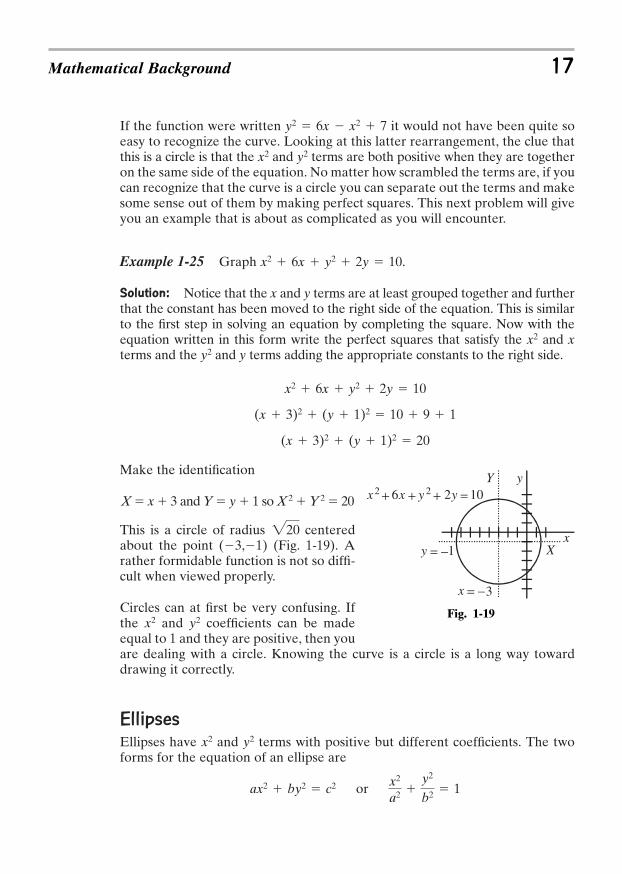
Example 1-25 Graph .
Solution: Notice that the x and y terms are at least grouped together and furtherthat the constant has been moved to the right side of the equation. This is similarto the first step in solving an equation by completing the square. Now with theequation written in this form write the perfect squares that satisfy the and xterms and the and y terms adding the appropriate constants to the right side.
Make the identification
X x 3 and Y y 1 so X 2 Y 2 20
This is a circle of radius centeredabout the point (3,1) (Fig. 1-19). Arather formidable function is not so diffi-cult when viewed properly.
Circles can at first be very confusing. Ifthe and coefficients can be madeequal to 1 and they are positive, then youare dealing with a circle. Knowing the curve is a circle is a long way towarddrawing it correctly.
Ellipses
Ellipses have and terms with positive but different coefficients. The twoforms for the equation of an ellipse are
or x2
a2 y2
b2 1ax2 by2 c2
y2x2
y2x2
220
(x 3)2 (y 1)2 20
(x 3)2 (y 1)2 10 9 1
x2 6x y2 2y 10
y2x2
x2 6x y2 2y 10
y2x2
y2 6x x2 7
Mathematical Background 17
Fig. 1-19
x x y y2 6 2 10+ + + =
xX
yY
x = −3
y = −1
2
Each form has its advantages with the latter form being the more convenientfor graphing.
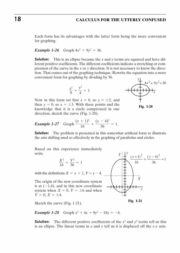
Example 1-26 Graph .
Solution: This is an ellipse because the x and y terms are squared and have dif-ferent positive coefficients. The different coefficients indicate a stretching or com-pression of the curve in the x or y direction. It is not necessary to know the direc-tion. That comes out of the graphing technique. Rewrite the equation into a moreconvenient form for graphing by dividing by 36.
Now in this form set first so , andthen , so . With these points and theknowledge that it is a circle compressed in onedirection, sketch the curve (Fig. 1-20).
Example 1-27 Graph .
Solution: The problem is presented in this somewhat artificial form to illustratethe axis shifting used so effectively in the graphing of parabolas and circles.
Based on this experience immediatelywrite
with the definitions , Y y 4.
The origin of the new coordinate systemis at (1,4), and in this new coordinatesystem when and when
, .
Sketch the curve (Fig. 1-21).
Example 1-28 Graph x2 4x 9y2 18y 4.
Solution: The different positive coefficients of the and terms tell us thisis an ellipse. The linear terms in x and y tell us it is displaced off the x-y axis.
y2x2
X 4Y 0Y 6X 0,
X x 1
X 2
16
Y 2
36 1
(x 1)2
16
(y 4)2
36 1
x 3y 0y 2x 0,
x2
9 y2
4 1
4x2 9y2 36
18 CALCULUS FOR THE UTTERLY CONFUSED
Fig. 1-21
Fig. 1-20
x
y4 9 362 2x y+ =
x
y
X
Y1
36
)4(
16
)1( 22
=−++ yx
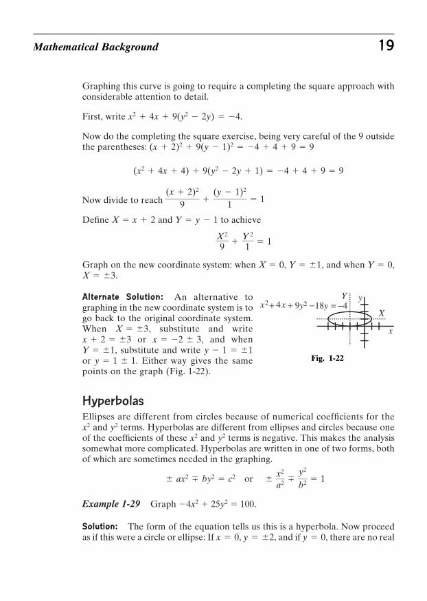
Graphing this curve is going to require a completing the square approach withconsiderable attention to detail.
First, write .
Now do the completing the square exercise, being very careful of the 9 outsidethe parentheses:
Now divide to reach
Define and to achieve
Graph on the new coordinate system: when , , and when ,.
Alternate Solution: An alternative tographing in the new coordinate system is togo back to the original coordinate system.When , substitute and write
or , and when, substitute and write
or . Either way gives the samepoints on the graph (Fig. 1-22).
Hyperbolas
Ellipses are different from circles because of numerical coefficients for theand terms. Hyperbolas are different from ellipses and circles because one
of the coefficients of these and terms is negative. This makes the analysissomewhat more complicated. Hyperbolas are written in one of two forms, bothof which are sometimes needed in the graphing.
or
Example 1-29 Graph 4x2 25y2 100.
Solution: The form of the equation tells us this is a hyperbola. Now proceedas if this were a circle or ellipse: If , , and if , there are no realy 0y 2x 0
x2
a2 7y2
b2 1 ax2 7 by2 c2
y2x2y2x2
y 1 1y 1 1Y 1
x 2 3x 2 3X 3
X 3Y 0Y 1X 0
X 2
9 Y 2
1 1
Y y 1X x 2
(x 2)2
9 (y 1)2
1 1
(x2 4x 4) 9(y2 2y 1) 4 4 9 9
(x 2)2 9(y 1)2 4 4 9 9
x2 4x 9(y2 2y) 4
Mathematical Background 19
Fig. 1-22
x
y
X
Yx x2 4 18y =+ + 9y2 − −4
values of x. If the curve goes through the points and and does notexist along the line , then the curve must have two separate parts!Rearrange the equation to and note immediately that for realvalues of x, y has to be greater than 2 or less than 2. The curve does not existin the region bounded by the lines and .
At this point in the analysis we have two points and a region where the curvedoes not exist. Further analysis requires a departure from the usual techniquesapplied to conics. Rewrite the equation again, but this time in the form y …
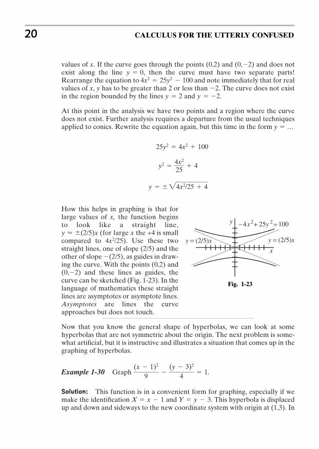
How this helps in graphing is that forlarge values of x, the function beginsto look like a straight line,
(for large x the +4 is smallcompared to ). Use these twostraight lines, one of slope and theother of slope (2/5), as guides in draw-ing the curve. With the points and
and these lines as guides, thecurve can be sketched (Fig. 1-23). In thelanguage of mathematics these straightlines are asymptotes or asymptote lines.Asymptotes are lines the curveapproaches but does not touch.
Now that you know the general shape of hyperbolas, we can look at somehyperbolas that are not symmetric about the origin. The next problem is some-what artificial, but it is instructive and illustrates a situation that comes up in thegraphing of hyperbolas.
Example 1-30 Graph .
Solution: This function is in a convenient form for graphing, especially if wemake the identification and . This hyperbola is displacedup and down and sideways to the new coordinate system with origin at (1,3). In
Y y 3X x 1
(x 1)2
9 (y 3)2
4 1
(0,2)(0,2)
(2/5)4x2/25
y < (2/5)x
y 24x2/25 4
y2 4x2
25 4
25y2 4x2 100
y 2y 2
4x2 25y2 100y 0
(0,2)(0,2)
20 CALCULUS FOR THE UTTERLY CONFUSED
Fig. 1-23
x
y =4 25y 1002 2x
y = (2/5)xy = (2/5)x
+_
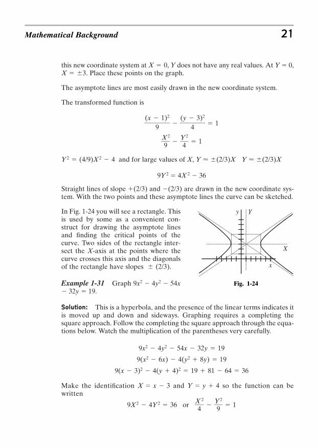
this new coordinate system at , Y does not have any real values. At Y 0,. Place these points on the graph.
The asymptote lines are most easily drawn in the new coordinate system.
The transformed function is
and for large values of X,
9Y 2 4X 2 36
Straight lines of slope (2/3) and (2/3) are drawn in the new coordinate sys-tem. With the two points and these asymptote lines the curve can be sketched.
In Fig. 1-24 you will see a rectangle. Thisis used by some as a convenient con-struct for drawing the asymptote linesand finding the critical points of thecurve. Two sides of the rectangle inter-sect the X-axis at the points where thecurve crosses this axis and the diagonalsof the rectangle have slopes .
Example 1-31 Graph 9x2 4y2 54x 32y 19.
Solution: This is a hyperbola, and the presence of the linear terms indicates itis moved up and down and sideways. Graphing requires a completing thesquare approach. Follow the completing the square approach through the equa-tions below. Watch the multiplication of the parentheses very carefully.
Make the identification and so the function can bewritten
or X2
4 Y 2
9 19X 2 4Y 2 36
Y y 4X x 3
9(x 3)2 4(y 4)2 19 81 64 36
9(x2 6x) 4(y2 8y) 19
9x2 4y2 54x 32y 19
(2/3)
Y < (2/3)XY < (2/3)XY 2 (4/9)X 2 4
X 2
9 Y 2
4 1
(x 1)2
9 (y 3)2
4 1
X 3X 0
Mathematical Background 21
Fig. 1-24
x
y
X
Y
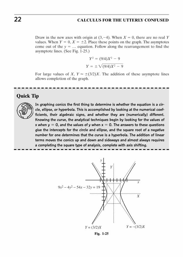
Draw in the new axes with origin at . When X 0, there are no real Yvalues. When , . Place these points on the graph. The asymptotescome out of the y … equation. Follow along the rearrangement to find theasymptote lines. (See Fig. 1-25.)
For large values of X, . The addition of these asymptote linesallows completion of the graph.
Y < (3/2)X
Y 2(9/4)X 2 9
Y 2 (9/4)X 2 9
X 2Y 0(3,4)
22 CALCULUS FOR THE UTTERLY CONFUSED
Quick Tip
In graphing conics the first thing to determine is whether the equation is a cir-
cle, ellipse, or hyperbola. This is accomplished by looking at the numerical coef-
ficients, their algebraic signs, and whether they are (numerically) different.
Knowing the curve, the analytical techniques begin by looking for the values of
x when y 0, and the values of y when x 0. The answers to these questions
give the intercepts for the circle and ellipse, and the square root of a negative
number for one determines that the curve is a hyperbola. The addition of linear
terms moves the conics up and down and sideways and almost always requires
a completing the square type of analysis, complete with axis shifting.
Fig. 1-25
x
y
X
Y
Y = (3/2)X Y = −(3/2)X
9x2 − 4y2 − 54x − 32y = 19
If you can figure out what the curve looks like and can find the intercepts (and ) you are a long way toward graphing the function. The shifting ofaxes just takes attention to detail.
1-8 Graphing Trigonometric FunctionsGraphing the trigonometric functions does not usually present any prob-lems. There are a few pitfalls, but with the correct graphing technique thesecan be avoided. Before graphing the functions you need to know their gen-eral shape. The trigonometric relations are defined in an earlier section andtheir functions shown graphically. If you are not very familiar with the shapeof the sine, cosine, and tangent functions draw them out on a 3 5 card anduse this card as a bookmark in your text or study guide and review it everytime you open your book (possibly even more often) until the word sineprojects an image of a sine function in your mind, and likewise for cosineand tangent.
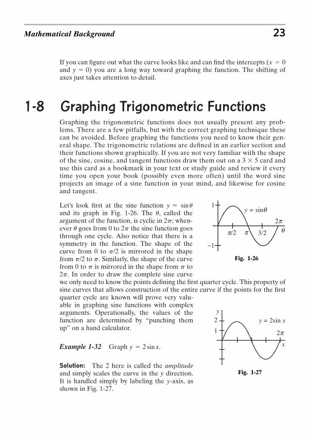
Let’s look first at the sine function and its graph in Fig. 1-26. The , called theargument of the function, is cyclic in ; when-ever goes from 0 to the sine function goesthrough one cycle. Also notice that there is asymmetry in the function. The shape of thecurve from 0 to is mirrored in the shapefrom to . Similarly, the shape of the curvefrom 0 to is mirrored in the shape from to
. In order to draw the complete sine curvewe only need to know the points defining the first quarter cycle. This property ofsine curves that allows construction of the entire curve if the points for the firstquarter cycle are known will prove very valu-able in graphing sine functions with complexarguments. Operationally, the values of thefunction are determined by “punching themup” on a hand calculator.
Example 1-32 Graph .
Solution: The 2 here is called the amplitudeand simply scales the curve in the y direction.It is handled simply by labeling the y-axis, asshown in Fig. 1-27.
y 2 sin x
2ppp
pp/2p/2
2pu
2pu
y sin u
y 0x 0
Mathematical Background 23
Fig. 1-27
Fig. 1-26
y = sinq
2p
p/2 3/2
1
−1
p q
x
2p1
y = 2sin x2y
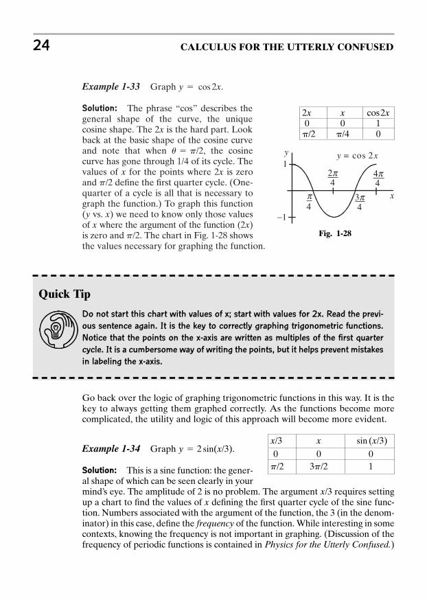
Example 1-33 Graph .
Solution: The phrase “cos” describes thegeneral shape of the curve, the uniquecosine shape. The is the hard part. Lookback at the basic shape of the cosine curveand note that when , the cosinecurve has gone through of its cycle. Thevalues of x for the points where 2x is zeroand define the first quarter cycle. (One-quarter of a cycle is all that is necessary tograph the function.) To graph this function(y vs. x) we need to know only those valuesof x where the argument of the function ( )is zero and . The chart in Fig. 1-28 showsthe values necessary for graphing the function.
p/22x
p/2
1/4u p/2
2x
y cos 2x
24 CALCULUS FOR THE UTTERLY CONFUSED
Quick Tip
Do not start this chart with values of x; start with values for 2x. Read the previ-
ous sentence again. It is the key to correctly graphing trigonometric functions.
Notice that the points on the x-axis are written as multiples of the first quarter
cycle. It is a cumbersome way of writing the points, but it helps prevent mistakes
in labeling the x-axis.
Go back over the logic of graphing trigonometric functions in this way. It is thekey to always getting them graphed correctly. As the functions become morecomplicated, the utility and logic of this approach will become more evident.
Example 1-34 Graph .
Solution: This is a sine function: the gener-al shape of which can be seen clearly in yourmind’s eye. The amplitude of 2 is no problem. The argument requires settingup a chart to find the values of x defining the first quarter cycle of the sine func-tion. Numbers associated with the argument of the function, the 3 (in the denom-inator) in this case, define the frequency of the function. While interesting in somecontexts, knowing the frequency is not important in graphing. (Discussion of thefrequency of periodic functions is contained in Physics for the Utterly Confused.)
x/3
y 2 sin(x/3)
2x x cos2x0 0 1
/2 /4 0
x
0 0 013p/2p/2
sin (x/3)x/3
Fig. 1-28
x
y
4
2p
3pp 4
4
4p 4
y = cos 2x1
−1
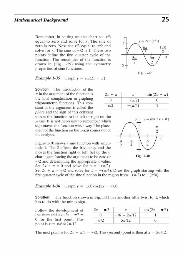
Remember, in setting up the chart set equal to zero and solve for x. The sine ofzero is zero. Next set equal to andsolve for x. The sine of is 1. These twopoints define the first quarter cycle of thefunction. The remainder of the function isdrawn in (Fig. 1-29) using the symmetryproperties of sine functions.
Example 1-35 Graph .
Solution: The introduction of thep in the argument of the function isthe final complication in graphingtrigonometric functions. This con-stant in the argument is called thephase and the sign of this constantmoves the function to the left or right on thex-axis. It is not necessary to remember whichsign moves the function which way. The place-ment of the function on the x-axis comes out ofthe analysis.
Figure 1-30 shows a sine function with ampli-tude 1. The 2 affects the frequency and themoves the function right or left. Set up the pchart again forcing the argument to be zero or
and determining the appropriate x value.Set and solve for .Set and solve for . Draw the graph starting with thefirst quarter cycle of the sine function in the region from to .
Example 1-36 Graph .
Solution: The function shown in Fig. 1-31 has another little twist to it, whichhas to do with the minus sign.
Follow the development ofthe chart and take 2x p/3 0 for the first point. Thispoint is .
The next point is for . This (second) point is then at .x 5p/122x p/3 p/2
x p/6 or 2p/12
y (1/3) cos (2x p/3)
(p/4)(p/2)x (p/4)2x p p/2x (p/2)2x p 0
p/2
y sin(2x p)
p/2p/2x/3
x/3
Mathematical Background 25
Fig. 1-29
Fig. 1-30
0 01(p/4)p/2
(p/2)sin (2x p)x2x p
0 105p/12p/2
p/6 2p/12cos (2x p/3)x2x p/3
3p 2
9p 2
12p2
6p 2
2 y = 2sin(x/3)
x
y
−2
x
y )2sin( += xy
2
442
p
p
ppp __
Set up the x-y coordinate system and placethe first quarter of the cosine functionbetween and . With this sectionof the cosine function complete, draw in theremainder of the curve.
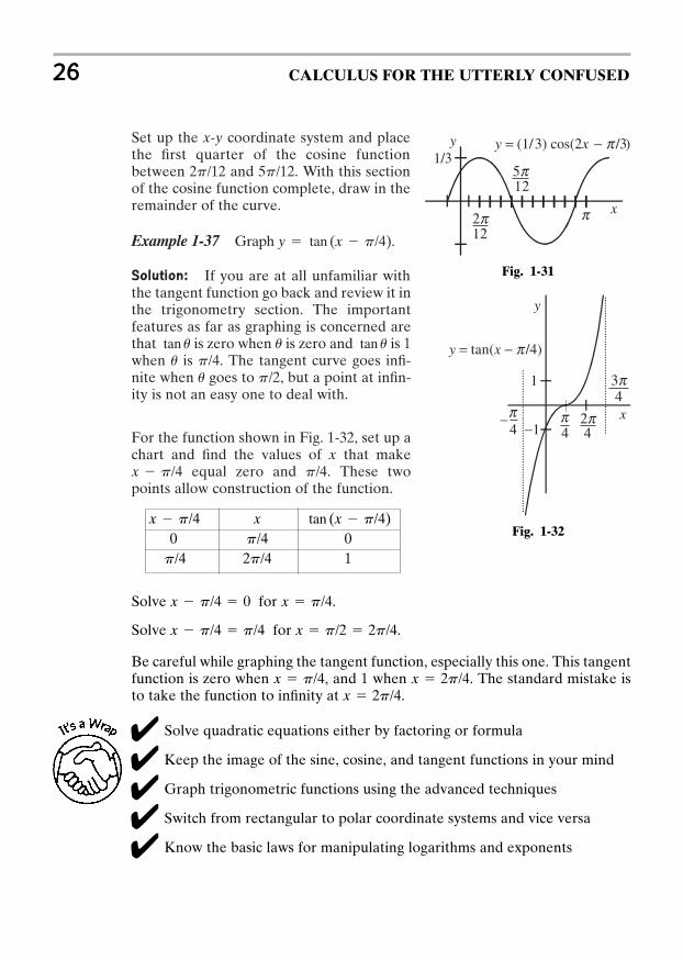
Example 1-37 Graph .
Solution: If you are at all unfamiliar withthe tangent function go back and review it inthe trigonometry section. The importantfeatures as far as graphing is concerned arethat is zero when is zero and is 1when is . The tangent curve goes infi-nite when goes to , but a point at infin-ity is not an easy one to deal with.
For the function shown in Fig. 1-32, set up achart and find the values of x that make
equal zero and . These twopoints allow construction of the function.
p/4x p/4
p/2u
p/4u
tan uutan u
y tan (x p/4)
5p/122p/12
26 CALCULUS FOR THE UTTERLY CONFUSED
Solve for .
Solve for .
Be careful while graphing the tangent function, especially this one. This tangentfunction is zero when , and 1 when . The standard mistake isto take the function to infinity at .
Solve quadratic equations either by factoring or formula
Keep the image of the sine, cosine, and tangent functions in your mind
Graph trigonometric functions using the advanced techniques
Switch from rectangular to polar coordinate systems and vice versa
Know the basic laws for manipulating logarithms and exponents
x 2p/4x 2p/4x p/4
x p/2 2p/4x p/4 p/4
x p/4x p/4 0
x0 0
12p/4p/4p/4
tan (x p/4)x p/4
Fig. 1-31
x
y1/3
2p12
5p12
y = (1/3) cos(2x − p /3)
p
Fig. 1-32
x
y
42p 4
1
−1
y = tan(x − p /4)
4
3p 4
p p_
Evaluate and graph functions
Graph circles (equal and positive coefficients of the x2 and y2 terms)
Graph ellipses (nonequal and positive coefficients of the x2 and y2 terms)
Graph hyperbolas (nonequal and one “” sign of the x2 and y2 terms)
PROBLEMS
1. Solve by factoring .2. Solve by factoring .3. Solve by quadratic formula .4. Solve by quadratic formula .5. Write using the binomial expansion.6. Convert p/4 rad to degrees.7. Convert 0.45 rad to degrees.8. Convert 2.6 rad to degrees.9. Convert 80 to radians.
10. Convert 200 to radians.11. Switch the point (4,6) to polar form.12. Switch the point (2,5) to polar form.13. Switch 3 @ 20 to rectangular form.14. Switch 5 @ 60 to rectangular form.15. Solve 6 ln3x for x.16. Solve .17. Solve .18. Write log3 = 0.48 in exponential form.19. Solve .20. Evaluate log(3.6)(4.1)3.21. Evaluate log[(4.2)2/2.3].22. What is the y intercept for the function ?23. What is the y intercept for the function ?24. Graph .25. Graph .26. Graph .27. Graph .28. Graph .29. Graph .30. Graph .31. Graph 32. Graph .33. Graph .y cos (3x p/3)
y tan (x p/2)y 2 sin (2x p/2).4y2 16x2 649x2 4y2 364x2 25y2 100x2 2x y2 4y 1(x 2)2 (y 3)2 9y x2 6x 9y x2 2x 8
y x2 3y 3x 2
10x 0.56
e2x 6.8ex 4.3
(a b)32x2 5x 6 0x2 7x 3 0
2x2 7x 4 0x2 3x 10 0
Mathematical Background 27
ANSWERS
1.2.
3.
4.
5.
6.
7.
8.
9.
10.
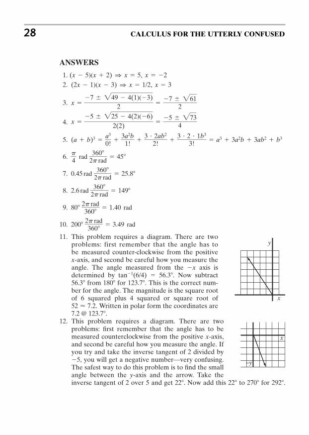
11. This problem requires a diagram. There are twoproblems: first remember that the angle has tobe measured counter-clockwise from the positivex-axis, and second be careful how you measure theangle. The angle measured from the x axis isdetermined by tan1(6/4) 56.3. Now subtract56.3 from 180 for 123.7. This is the correct num-ber for the angle. The magnitude is the square rootof 6 squared plus 4 squared or square root of
. Written in polar form the coordinates are7.2 @ 123.7.
12. This problem requires a diagram. There are twoproblems: first remember that the angle has to bemeasured counterclockwise from the positive x-axis,and second be careful how you measure the angle. Ifyou try and take the inverse tangent of 2 divided by5, you will get a negative number—very confusing.The safest way to do this problem is to find the smallangle between the y-axis and the arrow. Take theinverse tangent of 2 over 5 and get 22. Now add this 22 to 270 for 292.
52 < 7.2
2002p rad360
3.49 rad
802p rad360
1.40 rad
2.6 rad360
2p rad 149
0.45 rad360
2p rad 25.8
p4 rad
3602p rad
45
(a b)3 a3
0!
3a2b1!
3 2ab2
2!
3 2 1b3
3! a3 3a2b 3ab2 b3
x 5 225 4(2)(6)
2(2)
5 2734
x 7 249 4(1)(3)
2 7 261
2
(2x 1)(x 3) 1 x 1/2, x 3(x 5)(x 2) 1 x 5, x 2
28 CALCULUS FOR THE UTTERLY CONFUSED
y
x
-y
x
The magnitude of the arrow is the square root of 2squared and 5 squared, or square root of .Written in polar form the coordinates are 5.4 @ 292.
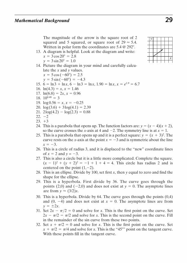
13. A diagram is helpful. Look at the diagram and write:
14. Picture the diagram in your mind and carefully calcu-late the x and y values.
15. 6 ln3 lnx, 6 ln3 lnx, 1.90 lnx, x e1.9 6.716. ln(4.3) x, x 1.4617. ln(6.8) 2x, x 0.9618.19. log 0.56 x, x 0.2520. log(3.6) 3log(4.1) 2.3921. 2log(4.2) log(2.3) 0.8822. 223. 324. This is a parabola that opens up. The function factors are: y (x 4)(x 2),
so the curve crosses the x-axis at 4 and 2. The symmetry line is at x 1.25. This is a parabola that opens up and it is a perfect square: . The
curve rests on the x-axis at the point x 3 and is symmetric about the linex 3.
26. This is a circle of radius 3, and it is displaced to the “new” coordinate linesof x 2 and y = 3.
27. This is also a circle but it is a little more complicated. Complete the square.. This circle has radius 2 and is
centered on the point (1,2).28. This is an ellipse. Divide by 100, set first x, then y equal to zero and find the
shape for the ellipse.29. This is a hyperbola. First divide by 36. The curve goes through the
points (2,0) and (2,0) and does not exist at y 0. The asymptote linesare from .
30. This is a hyperbola. Divide by 64. The curve goes through the points (0,4)and (0, 4) and does not exist at x 0. The asymptote lines are from
.31. Set and solve for x. This is the first point on the curve. Set
and solve for x. This is the second point on the curve. Fillin the remainder of the sin curve from these two points.
32. Set and solve for x. This is the first point on the curve. Setand solve for x. This is the “45” point on the tangent curve.
With these points fill in the tangent curve.x p/2 p/4
x p/2 0
2x p/2 p/22x p>2 0
y 2x
y < (3/2)x
(x 1)2 (y 2)2 1 1 4 4
y (x 3)2
100.48 3
y 5 sin (60) 4.3x 5 cos (60) 2.5
y 3 sin 20 1.0x 3 cos 20 2.8
29 < 5.4
Mathematical Background 29
y
x
30 CALCULUS FOR THE UTTERLY CONFUSED
33. Set and solve for x. This is the first point for the cos curve.Set and solve for x. This is the point needed to completethe first quarter of the cos curve. Then fill in the rest of the cos curve.
3x p/3 p/23x p/3 0
My favorite is completing thesquare.
My favorite is graphing hyperbolas.
CHAPTER 2
LIMITS ANDCONTINUITY
You should read this chapter if you need to review or you need to learn about
The concept of a limit
Algebraic techniques for finding limits
Discontinuities
Using discontinuities in graphing
31
Copyright © 2007 by The McGraw-Hill Companies, Inc. Click here for terms of use.
The concept of the limit in calculus is very important. It describes what happensto a function as a particular value is approached. The derivative, one of themajor themes of calculus, is defined in limit terms. This short chapter will helpyou to think in terms of limits. The first thing to understand about limits is thata limit of a function is not the value of the function. The change in thinking(from value to limit) is important because most functions are understood as aseries of mathematical operations that can be evaluated at certain points simplyby substitution.
The (polynomial) function can be evaluated for any real num-ber: replace x with the number and perform the indicated operations. Askingthe limit of this function as x approaches 2, for example, is an uninterestingquestion. The function can be evaluated at 2 or any point arbitrarily close to 2by substituting and performing the operations.
Other functions, such as polynomial fractions, cannot be evaluated at certainpoints and these functions are best understood by thinking in terms of limits.The function can be evaluated for any real numberexcept 2. Replacing x by 2 produces the meaningless statement 0/0.Remember that any number times 0 is 0, but any number divided by 0 is“meaningless” (including 0/0). Looking at the limit of the function, as xapproaches 2, tells us about the function in the vicinity of 2. The limit ofthe function is a convenient phrase for the question, “What happens to thefunction as a certain value is approached?” Writing this in mathematical nota-tion we get the following:
The notation in front of the functions is read the limit, as x approaches minustwo. In the case of rational functions, factoring and reducing the fraction helpsin finding the limit.
Finding the limit of this function as helps in understanding the func-tion. Since the original function gives the meaningless 0/0 at the point wherex 2, the function cannot exist, “does not have meaning,” at x 2.Graphing the function illustrates this point. The (simplified) function
is a straight line of slope 1 and intercept 2. The functionis also a straight line of slope 1 and intercept 2, but it
does not exist at the point where x 2. This nonexistence at x 2 is illus-trated on the graph in Fig. 2-1 with the open circle.
y (x2 4)/(x 2)y x 2
x S 2
limxS2
x24x 2 lim
xS2
(x 2)(x 2)x 2 lim
xS2(x 2) 4
y (x2 4)/(x 2)
y x2 2x 3
32 CALCULUS FOR THE UTTERLY CONFUSED

Example 2-1 Find the limit of as .
Solution: At the fraction is 0/0, so perform some algebra on the fractionbefore taking the limit.
As an exercise graph the original function, showing the nonexistence at .
Another category of function that is understoodwith the help of limits is polynomial fractions,where the higher power polynomial is in thedenominator rather than the numerator. The sim-plest function to look at is . (The productof two variables equaling a constant describes cer-tain relationships. For example, pressure andvolume for a fixed amount of gas at constant tem-perature is described by the cost ofcomparable real estate times the commuting dis-tance from a major commercial center is describedby RD const.)
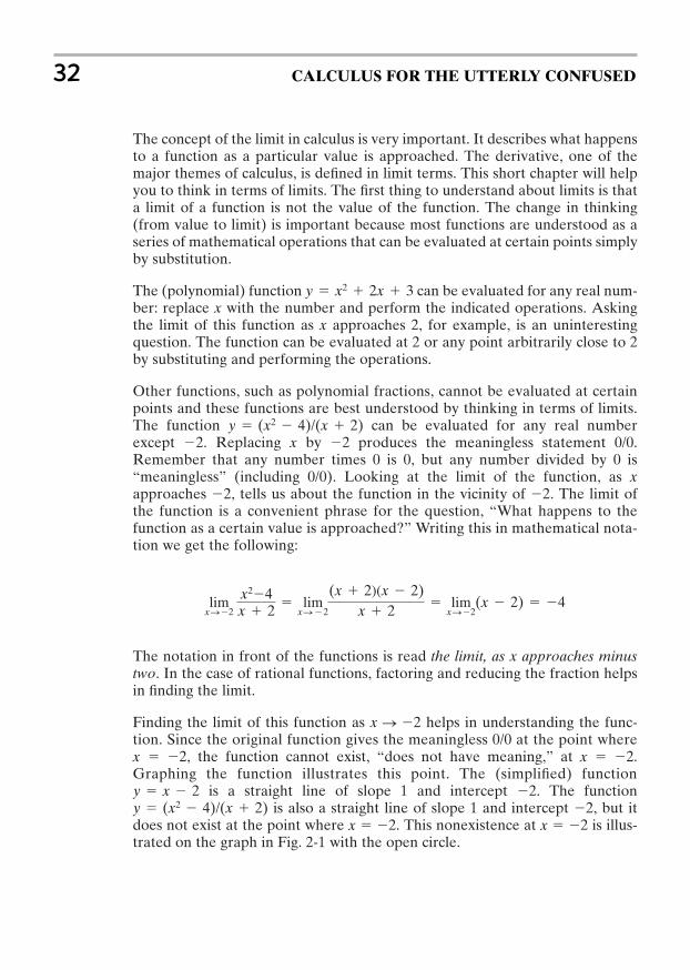
This relationship or is bestunderstood in the context of its graph.Numbers can be assigned to x, and y values cal-culated but note how the concept and languageof limits make graphing so much easier. Referto Fig. 2-2 during this discussion. First considerpositive values. The point , is soeasy to calculate it should not be ignored. Thecurve goes through this point. Now as x is madea larger and larger positive number, y approacheszero, but remains positive. This can be expressedin a simple sentence.
As x approaches plus infinity, y approacheszero, but remains positive or in mathematical symbolism,
Write the situation for small values of x directly in mathematical symbolism,
As x S 0, y S `
As x S `, y S 0
y 1x 1
y 1/xxy 1
pV const;
y 1/x
x 1
limxS1
x2 x 2x 1
limxS1
(x 2)(x 1)x 1
limxS1
(x 2) 3
x 1
x S 1y (x2 x 2)/(x 1)
Limits and Continuity 33
Fig. 2-1
Fig. 2-2
x
y y = x2 − 4x + 2
x
y
y = 1/x
What we are saying here is that if x is a very, very, very small number, evensmaller than 0.000000001, the 1 divided by this number is a very, very, very largenumber. So as .
With this information, the positive portion of the graph can be drawn. In thecase of pressure and volume or cost of real estate and distance, the problem dic-tates only positive values. In the function no such restriction exists.
Refer to the graph in Fig. 2-2 and follow the logic and symbolism in the statements
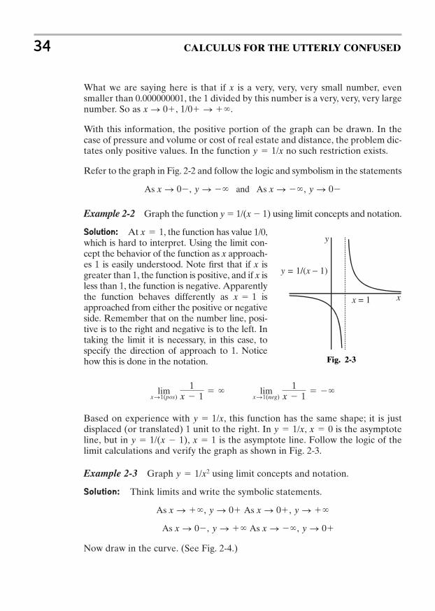
Example 2-2 Graph the function y 1/(x 1) using limit concepts and notation.
Solution: At , the function has value 1/0,which is hard to interpret. Using the limit con-cept the behavior of the function as x approach-es 1 is easily understood. Note first that if x isgreater than 1, the function is positive, and if x isless than 1, the function is negative. Apparentlythe function behaves differently as isapproached from either the positive or negativeside. Remember that on the number line, posi-tive is to the right and negative is to the left. Intaking the limit it is necessary, in this case, tospecify the direction of approach to 1. Noticehow this is done in the notation.
Based on experience with , this function has the same shape; it is justdisplaced (or translated) 1 unit to the right. In , is the asymptoteline, but in , is the asymptote line. Follow the logic of thelimit calculations and verify the graph as shown in Fig. 2-3.
Example 2-3 Graph using limit concepts and notation.
Solution: Think limits and write the symbolic statements.
Now draw in the curve. (See Fig. 2-4.)
As x S `, y S 0As x S 0, y S `
As x S 0, y S `As x S `, y S 0
y 1/x2
x 1y 1/(x 1)x 0y 1/x
y 1/x
limxS1(pos)
1x 1
` limxS1(neg)
1x 1
`
x 1
x 1
As x S 0, y S ` and As x S `, y S 0
y 1/x
1/0 S `x S 0,
34 CALCULUS FOR THE UTTERLY CONFUSED
Fig. 2-3
x
y
y = 1/(x − 1)
x = 1
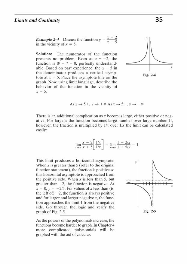
Example 2-4 Discuss the function in the vicinity of .
Solution: The numerator of the functionpresents no problem. Even at , thefunction is , perfectly understand-able. Based on past experience, the inthe denominator produces a vertical asymp-tote at . Place the asymptote line on thegraph. Now, using limit language, describe thebehavior of the function in the vicinity of
.
There is an additional complication as x becomes large, either positive or neg-ative. For large x the function becomes large number over large number. If,however, the fraction is multiplied by over the limit can be calculatedeasily:
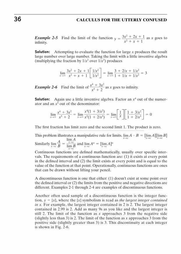
This limit produces a horizontal asymptote.When x is greater than 5 (refer to the originalfunction statement), the fraction is positive sothis horizontal asymptote is approached fromthe positive side. When x is less than 5, butgreater than 2, the function is negative. At
, . For values of x less than (tothe left of) 2, the function is always positiveand for larger and larger negative x, the func-tion approaches the limit 1 from the negativeside. Go through the logic and verify thegraph of Fig. 2-5.
As the powers of the polynomials increase, thefunctions become harder to graph. In Chapter 4more complicated polynomials will begraphed with the aid of calculus.
y 2/5x 0
limxS`
x 2x 5
B1/x1/xR lim
xS`
1 2/x1 5/x
1
1/x1/x
As x S 5, y S `As x S 5, y S `
x 5
x 5
x 50/ 7 0
x 2
x 5y
x 2x 5
Limits and Continuity 35
Fig. 2-4
Fig. 2-5
x
y
x
y
Example 2-5 Find the limit of the function as x goes toinfinity.
Solution: Attempting to evaluate the function for large x produces the resultlarge number over large number. Taking the limit with a little inventive algebra(multiplying the fraction by over ) produces
Example 2-6 Find the limit of as x goes to infinity.
Solution: Again use a little inventive algebra. Factor an out of the numer-ator and an out of the denominator:
The first fraction has limit zero and the second limit 1. The product is zero.
This problem illustrates a manipulative rule for limits.
Similarly and
Continuous functions are defined mathematically, usually over specific inter-vals. The requirements of a continuous function are: (1) it exists at every pointin the defined interval and (2) the limit exists at every point and is equal to thevalue of the function at that point. Operationally, continuous functions are onesthat can be drawn without lifting your pencil.
A discontinuous function is one that either: (1) doesn’t exist at some point overthe defined interval or (2) the limits from the positive and negative directions aredifferent. Examples 2-1 through 2-4 are examples of discontinuous functions.
Another often used sample of a discontinuous function is the integer func-tion, , where the symbolism is read as the largest integer containedin x. For example, the largest integer contained in 2 is 2. The largest integercontained in 2.99 is 2. Add as many 9s as you like and the largest integer isstill 2. The limit of the function as x approaches 3 from the negative side(slightly less than 3) is 2. The limit of the function as x approaches 3 from thepositive side (slightly greater than 3) is 3. This discontinuity at each integeris shown in Fig. 2-6.
[x]y [x]
limxSc
An [limxSc
A]nlimxSc
AB
lim AxSc
lim BxSc
limxSc
A B [limxSc
A][limxSc
B]
limxS`
x4 3x2
x5 2 lim
xS`
x4(1 3/x2)
x5(1 2/x5) lim
xS`B1
xR B1 3/x2
1 2/x5R 0
x5x4
x4 3x2
x5 2
limxS`
3x2 2x 1x2 x 1
B1/x2
1/x2R limxS`
3 2/x 1/x2
1 1/x 1/x2 3
1/x21/x2
y 3x2 2x 1x2 x 1
36 CALCULUS FOR THE UTTERLY CONFUSED
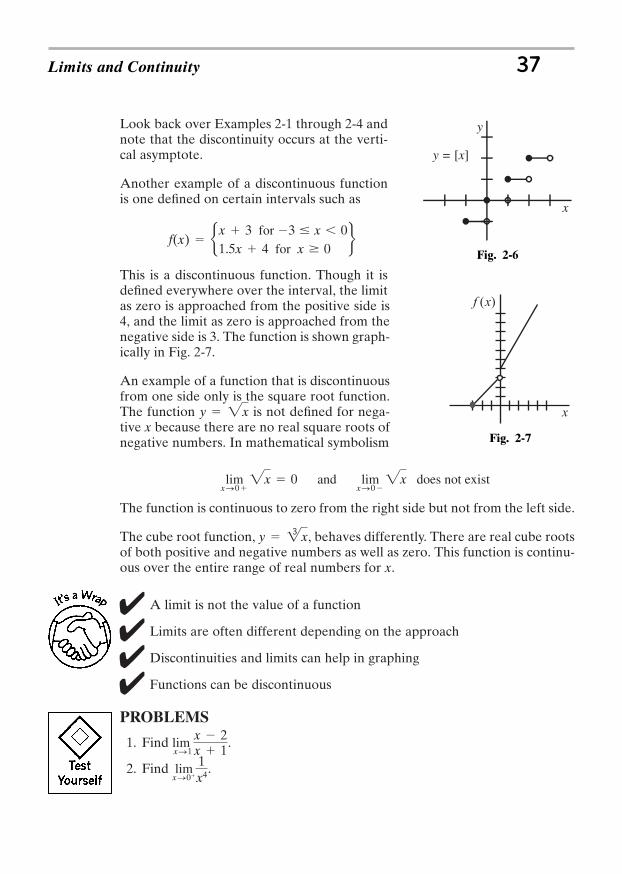
Look back over Examples 2-1 through 2-4 andnote that the discontinuity occurs at the verti-cal asymptote.
Another example of a discontinuous functionis one defined on certain intervals such as
This is a discontinuous function. Though it isdefined everywhere over the interval, the limitas zero is approached from the positive side is4, and the limit as zero is approached from thenegative side is 3. The function is shown graph-ically in Fig. 2-7.
An example of a function that is discontinuousfrom one side only is the square root function.The function is not defined for nega-tive x because there are no real square roots ofnegative numbers. In mathematical symbolism
The function is continuous to zero from the right side but not from the left side.
The cube root function, , behaves differently. There are real cube rootsof both positive and negative numbers as well as zero. This function is continu-ous over the entire range of real numbers for x.
A limit is not the value of a function
Limits are often different depending on the approach
Discontinuities and limits can help in graphing
Functions can be discontinuous
PROBLEMS
1. Find .
2. Find .limxS0
1x4
limxS1
x 2x 1
y 23 x
limxS0
2x 0 and limxS0
2x does not exist
y 2x
f(x) bx 3 for 3 x 01.5x 4 for x 0
r
Limits and Continuity 37
Fig. 2-6
x
y
y = [x]
Fig. 2-7
x
)(xf
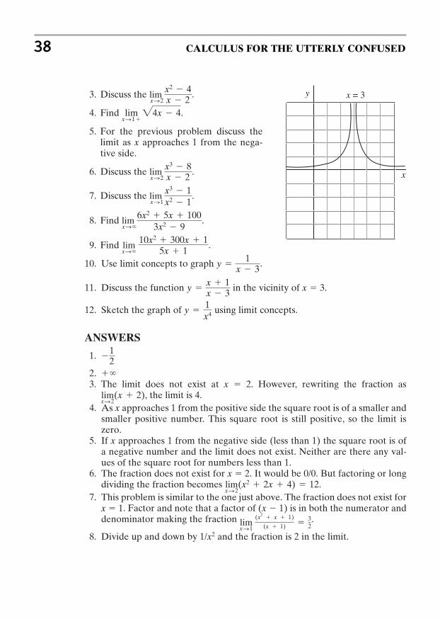
3. Discuss the .
4. Find .
5. For the previous problem discuss thelimit as x approaches 1 from the nega-tive side.
6. Discuss the .
7. Discuss the .
8. Find .
9. Find .
10. Use limit concepts to graph .
11. Discuss the function in the vicinity of x 3.
12. Sketch the graph of using limit concepts.
ANSWERS
1.
2.3. The limit does not exist at x 2. However, rewriting the fraction as
, the limit is 4.4. As x approaches 1 from the positive side the square root is of a smaller and
smaller positive number. This square root is still positive, so the limit iszero.
5. If x approaches 1 from the negative side (less than 1) the square root is ofa negative number and the limit does not exist. Neither are there any val-ues of the square root for numbers less than 1.
6. The fraction does not exist for x 2. It would be 0/0. But factoring or longdividing the fraction becomes .
7. This problem is similar to the one just above. The fraction does not exist forx 1. Factor and note that a factor of (x 1) is in both the numerator anddenominator making the fraction .
8. Divide up and down by 1/x2 and the fraction is 2 in the limit.
limxS1
(x2 x 1)
(x 1) 32
limxS2
(x2 2x 4) 12
limxS2
(x 2)
`
12
y 1x4
y x 1x 3
y 1
x 3
limxS`
10x2 300x 15x 1
limxS`
6x2 5x 1003x2 9
limxS1
x3 1x2 1
limxS2
x3 8x 2
limxS1
24x 4
limxS2
x2 4x 2
38 CALCULUS FOR THE UTTERLY CONFUSED
y
x
x = 3
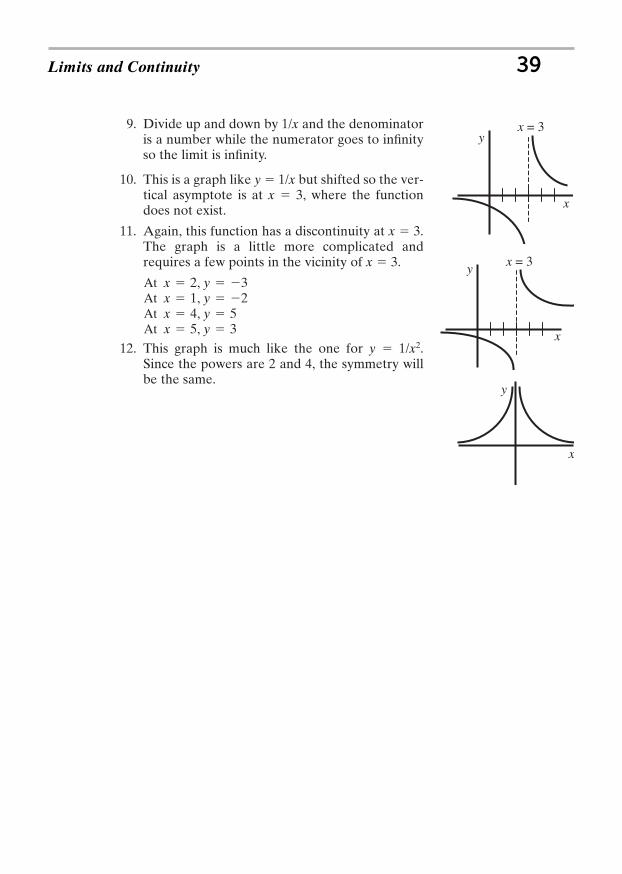
9. Divide up and down by 1/x and the denominatoris a number while the numerator goes to infinityso the limit is infinity.
10. This is a graph like y 1/x but shifted so the ver-tical asymptote is at x 3, where the functiondoes not exist.
11. Again, this function has a discontinuity at x 3.The graph is a little more complicated andrequires a few points in the vicinity of x 3.
12. This graph is much like the one for y 1/x2.Since the powers are 2 and 4, the symmetry willbe the same.
At x 5, y 3At x 4, y 5At x 1, y 2At x 2, y 3
Limits and Continuity 39
y
x
x = 3
x
yx = 3
y
x

This page intentionally left blank
CHAPTER 3
DERIVATIVES
You should read this chapter if you need to review or you need to learn about
Definition of the derivative
Derivatives of polynomials
Product and quotient rules
Trig, exponential, and Log functions
Implicit differentiation and the chain rule
Finding limits with derivatives
41
Copyright © 2007 by The McGraw-Hill Companies, Inc. Click here for terms of use.

The derivative of a function is the slope of that function anywhere the functionis well behaved. A function is well behaved in a region where there is a uniqueslope at every point. A constant function, , , is a straight line ofslope zero. A linear equation, , , has a constant slope(2 and 1 in these cases).
The simplest function that does not have a constant slope is the quadratic,(see Chapter 1 for a discussion of quadratics). The slope of the quadratic,
considering only positive values of x, increases as x increases. Look at a magni-fied portion of the curve and approximate the slope of the curve at anypoint by writing a general expression for the slope of the straight line connect-ing two points x and . The notation means a small change in x so thepoint is very close to x.x x
xx x
y x2
y x2
y x 5y 2x 3y 3y 2
42 CALCULUS FOR THE UTTERLY CONFUSED
Figure 3-1 shows the curve and the straight line connecting the points) and . The slope of the line between these
adjacent points is
The general expression for the slope of this curve at any point x is the limit ofthis approximate slope as goes to zero. Using the mathematical symbolismof limits, the general expression for the slope of is
This defining equation for the derivative is called , where the d notation indi-cates the limit of , or , or . For the quadratic, we have the following:f r(x)yr y/ x
dy/dx
dydx
yr f r(x) lim xS0
(x x)2 x2
x
y x2 x
(x x)2 x2
x
(x x, y (x x)2)(x, y x2y x2
2)( xxy + ∆=2)( xx∆y + ∆=
2xy =
2xy =
x xx + ∆∆x
2 - x
x
y
Fig. 3-1
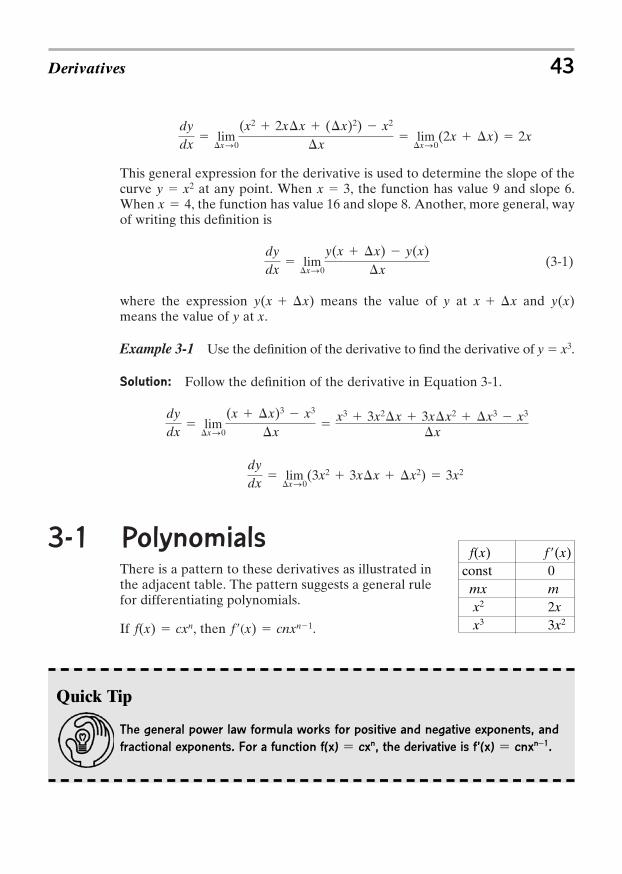
This general expression for the derivative is used to determine the slope of thecurve at any point. When , the function has value 9 and slope 6.When , the function has value 16 and slope 8. Another, more general, wayof writing this definition is
(3-1)
where the expression means the value of y at and means the value of y at x.
Example 3-1 Use the definition of the derivative to find the derivative of y x3.
Solution: Follow the definition of the derivative in Equation 3-1.
3-1 Polynomials There is a pattern to these derivatives as illustrated inthe adjacent table. The pattern suggests a general rulefor differentiating polynomials.
If , then .f r(x) cnxn1f(x) cxn
dydx
lim xS0
(3x2 3x x x2) 3x2
dydx
lim xS0
(x x)3 x3
x
x3 3x2 x 3x x2 x3 x3
x
y(x)x xy(x x)
dydx
lim xS0
y(x x) y(x) x
x 4x 3y x2
dydx
lim xS0
(x2 2x x ( x)2) x2
x lim
xS0(2x x) 2x
Derivatives 43
Quick Tip
The general power law formula works for positive and negative exponents, and
fractional exponents. For a function f(x) cxn, the derivative is f’(x) cnxn−1.
f(x) f(x)const 0
mx mx2 2xx3 3x2
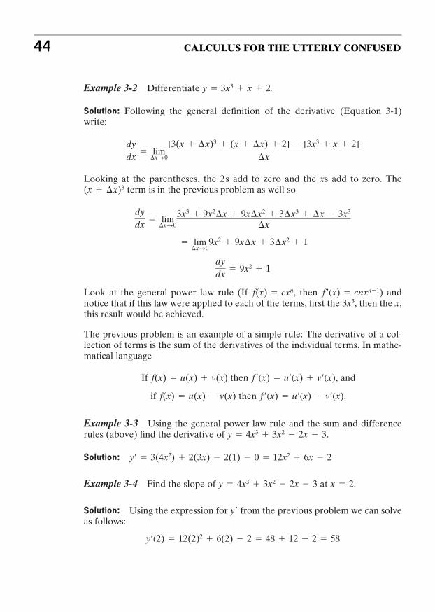
Example 3-2 Differentiate .
Solution: Following the general definition of the derivative (Equation 3-1)write:
Looking at the parentheses, the 2s add to zero and the xs add to zero. Theterm is in the previous problem as well so
Look at the general power law rule (If , then ) andnotice that if this law were applied to each of the terms, first the , then the x,this result would be achieved.
The previous problem is an example of a simple rule: The derivative of a col-lection of terms is the sum of the derivatives of the individual terms. In mathe-matical language
If then , and
if then .
Example 3-3 Using the general power law rule and the sum and differencerules (above) find the derivative of .
Solution:
Example 3-4 Find the slope of at .
Solution: Using the expression for y from the previous problem we can solveas follows:
yr(2) 12(2)2 6(2) 2 48 12 2 58
x 2y 4x3 3x2 2x 3
yr 3(4x2) 2(3x) 2(1) 0 12x2 6x 2
y 4x3 3x2 2x 3
f r(x) ur(x) vr(x)f(x) u(x) v(x)
f r(x) ur(x) vr(x)f(x) u(x) v(x)
3x3f r(x) cnxn1f(x) cxn
dydx
9x2 1
lim xS0
9x2 9x x 3 x2 1
dydx
lim xS0
3x3 9x2 x 9x x2 3 x3 x 3x3
x
(x x)3
dydx
lim xS0
[3(x x)3 (x x) 2] [3x3 x 2]
x
y 3x3 x 2
44 CALCULUS FOR THE UTTERLY CONFUSED
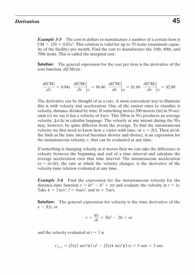
Example 3-5 The cost in dollars to manufacture x number of a certain item is. This relation is valid for up to 70 items (maximum capac-
ity of the facility) per month. Find the cost to manufacture the 10th, 40th, and70th items. This is called the marginal cost.
Solution: The general expression for the cost per item is the derivative of thecost function, .
The derivative can be thought of as a rate. A most convenient way to illustratethis is with velocity and acceleration. One of the easiest rates to visualize isvelocity, distance divided by time. If something moves 200 meters (m) in 50 sec-onds (s) we say it has a velocity of . This in produces an averagevelocity, in calculus language. The velocity at any instant during the may, however, be quite different from the average. To find the instantaneousvelocity we first need to know how x varies with time, or . Then ,the limit as the time interval becomes shorter and shorter, is an expression forthe instantaneous velocity, v, that can be evaluated at any time.
If something is changing velocity as it moves then we can take the difference invelocity between the beginning and end of a time interval and calculate theaverage acceleration over that time interval. The instantaneous acceleration( ), the rate at which the velocity changes, is the derivative of thevelocity-time relation evaluated at any time.
Example 3-6 Find the expression for the instantaneous velocity for thedistance-time function x kt 3 lt 2 mt and evaluate the velocity at t 1s.Take , and .
Solution: The general expression for velocity is the time derivative of thex f(t), or
and the velocity evaluated at t 1 is
v Zt1 (3) (2 m/s3)(1 s)2 (2) (4 m/s2)(1 s) 5 m/s 3 m/s
v dxdt
3kt2 2lt m
m 5 m/sl 4 m/s2k 2 m/s3,
a dv/dt
dx/dtx f(t)
50 s x/ t50 s200 m4 m/s
d(CM)dx
0.04xd(CM)
dx210
$0.40d(CM)
dx240
$1.60d(CM)
dx270
$2.80
d(CM)/dx
CM 120 0.02x2
Derivatives 45
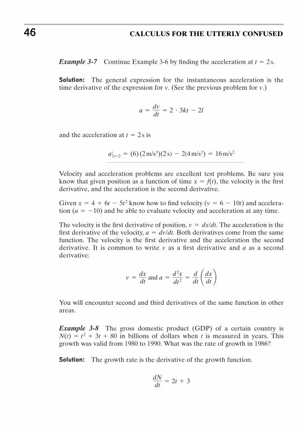
Example 3-7 Continue Example 3-6 by finding the acceleration at .
Solution: The general expression for the instantaneous acceleration is thetime derivative of the expression for v. (See the previous problem for v.)
and the acceleration at is
Velocity and acceleration problems are excellent test problems. Be sure youknow that given position as a function of time , the velocity is the firstderivative, and the acceleration is the second derivative.
Given know how to find velocity ( ) and accelera-tion ( ) and be able to evaluate velocity and acceleration at any time.
The velocity is the first derivative of position, . The acceleration is thefirst derivative of the velocity, . Both derivatives come from the samefunction. The velocity is the first derivative and the acceleration the secondderivative. It is common to write v as a first derivative and a as a secondderivative:
You will encounter second and third derivatives of the same function in otherareas.
Example 3-8 The gross domestic product (GDP) of a certain country isin billions of dollars when t is measured in years. This
growth was valid from 1980 to 1990. What was the rate of growth in 1986?
Solution: The growth rate is the derivative of the growth function.
dNdt
2t 3
N(t) t 2 3t 80
v dxdt
and a d 2xdt 2
ddt¢dx
dt≤
a dv/dtv dx/dt
a 10v 6 10tx 4 6t 5t 2
x f(t)
a Zt2 (6) (2 m/s3)(2 s) 2(4 m/s2) 16 m/s2
t 2 s
a dvdt
2 3kt 2l
t 2 s
46 CALCULUS FOR THE UTTERLY CONFUSED
and evaluating for 1986,
While the rate of growth is important the percentage of change is also impor-tant. In an absolute sense, a change of 50 in the manufacture of 500 items is a10% change while a change of 50 in 50,000 items is a 0.1% change. Change isrelative to the number of items manufactured. A 0.1% change will probablyrequire no change in manufacturing but a 10% change might have a significanteffect on manufacturing procedures. In order to get a measure of this relativechange we make the following definition.
This percentage rate of change is defined as
Example 3-9 For the previous problem find the percentage rate of change in1986.
Solution: The numerator of the fraction, dN/dt from the previous problem is:
The actual number for 1968 is:
The percentage rate of change is then,
In 1986 the GDP is 134 billion, the rate of growth is 15 billion per year and thepercentage rate of growth is 11% per year.
100 15134
11% per year
N(t) t 2 3t 80N(6) 62 3(6) 80
N 134 billion
dNdt26
15 billions per year
Percentage rate of change 100f r(x)f(x)
Percentage rate of change 100rate of change
size of quantity
dNdt26
2(6) 3 15 billion dollars per year.
Derivatives 47
3-2 Product and Quotient Rule Having established the derivatives of polynomials and worked some sampleproblems let’s move on to fractions and products.
Example 3-10 Find the derivative of the function .
Solution:
Second Solution: The solution could have been obtained much easier byapplying the rule for differentiating a product. The derivative of a product is thefirst term times the derivative of the second term plus the second term times thederivative of the first term. In mathematical symbolism,
For this problem, then,
dydx
x2 ddx
(x 2) (x 2) ddx
x2 x2(1) (x 2)(2x) 3x2 4x
If f(x) u(x)v(x) then f r(x) u(x)vr(x) ur(x)v(x)
dydx
3x2 4x
dydx
lim xS0
(x x)2(x x 2) x2(x 2) x
y x2(x 2)
48 CALCULUS FOR THE UTTERLY CONFUSED
dydx
lim xS0
(x3 x2 x 2x2 2x2 x 2x x2 4x x x x2 x3 2 x2) (x3 2x2) x
Quick Tip
In words the product rule is first × d (second) + second × d (first).
A similar, though somewhat more complicated rule applies for fractions.Again, use the basic definition of the derivative to find the differential of afraction and see how the differentiation can be performed much easier withthe fraction rule.
Example 3-11 Use the basic definition of the derivative to find dy/dx ofy x 1/x2.Solution:
Second Solution: The general rule for differentiating a fraction is:
By applying this rule the problem becomes much easier:
x2 2x
x4 x 2
x3
dydx
x2 d
dx(x 1) (x 1) d
dx(x2)
(x2)2 x2(1) (x 1)(2x)
x4
If f(x) u(x)v(x)
then f r(x) v(x)ur(x) u(x)vr(x)
[v(x)]2
dydx
x2 2x
x4 x 2
x3
dydx
lim xS0
x3 x2 x x2 (x3 2x2 x x x2 x2 2x x x2)(x x)2(x2)( x)
dydx
lim xS0
x2(x x 1) (x 1)(x2 2x x x2)(x x)2(x2)( x)
dydx
lim xS0
x x 1(x x)2
x 1x2
x
Derivatives 49
Quick Tip
In words the quotient rule is top × d (bottom) − bottom × d (top) all over (bottom)2.
3-3 Trigonometric FunctionsThere is no gereral rule for determining the derivative of trigonometric func-tions. Each trigonometric function has a unique derivative. One will be done todemonstrate the approach. Consult a table of derivatives for the derivative ofeach specific trigonometric function.
Example 3-12 Apply the basic definition to find the derivative of the sinefunction, .
Solution:
The can be replaced with the sum of two angles identity (see earliertrigonometric identities).
As goes to zero, goes to 1 (see the graph of the cosine function) sothe problem reduces to
As approaches zero, approaches . For small angles the sine functionlooks like a straight line of slope 1. Check this out with your hand calculator.
Take the sine of 0.2 (rad), a little over 11, and notice how close the sine of 0.2is to 0.2. Now decrease the angle to 0.1, 0.01, 0.001, until your calculator nolonger displays a difference between the sine and the angle. The limit of over as goes to zero is 1, so the derivative of the sine function is thecosine function.
The approximation sinu u for small u is used in many problems in physics andengineering.
3-4 Implicit DifferentiationThe general procedure for differentiating a polynomial function isto apply the power law rule to each term and write . Anotherand often very convenient way of looking at the problem would be to differen-tiate the entire equation term by term, , and then write
. You should notice that most differential tables are written inthis manner. As functions become more complicated differentiating term byterm like this and implicit differentiation become more convenient. Supposeyou have a function where it is impossible to solve for xin terms of y or y in terms of x. Implicit differentiation is the only way to find
.dy/dx
x4 x2y2 xy3 18
dy/dx 2x 2dy 2xdx 2dx
dy/dx 2x 2y x2 2x
u usin u
usin u u
dydu
cos u lim uS0
sin u u
cos u u
dydu
lim uS0
sin u cos u cos u sin u sin u u
sin(u u)
dydu
lim uS0
sin(u u) sin u
u
y sin u
50 CALCULUS FOR THE UTTERLY CONFUSED
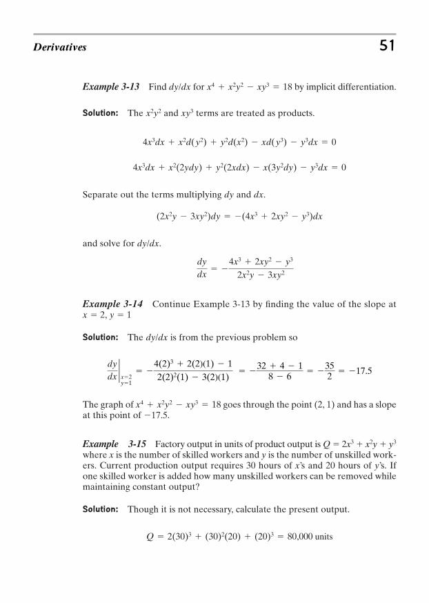
Example 3-13 Find for by implicit differentiation.
Solution: The and terms are treated as products.
Separate out the terms multiplying dy and dx.
and solve for .
Example 3-14 Continue Example 3-13 by finding the value of the slope atx 2, y 1
Solution: The is from the previous problem so
The graph of goes through the point (2, 1) and has a slopeat this point of 17.5.
Example 3-15 Factory output in units of product output is Q 2x3 x2y y3
where x is the number of skilled workers and y is the number of unskilled work-ers. Current production output requires 30 hours of x’s and 20 hours of y’s. Ifone skilled worker is added how many unskilled workers can be removed whilemaintaining constant output?
Solution: Though it is not necessary, calculate the present output.
Q 2(30)3 (30)2(20) (20)3 80,000 units
x4 x2y2 xy3 18
dydx2x2y1
4(2)3 2(2)(1) 12(2)2(1) 3(2)(1)
32 4 1
8 6
352 17.5
dy/dx
dydx
4x3 2xy2 y3
2x2y 3xy2
dy/dx
(2x2y 3xy2)dy (4x3 2xy2 y3)dx
4x3dx x2(2ydy) y2(2xdx) x(3y2dy) y3dx 0
4x3dx x2d(y2) y2d(x2) xd(y3) y3dx 0
xy3x2y2
x4 x2y2 xy3 18dy/dx
Derivatives 51
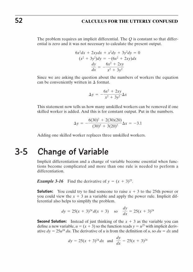
The problem requires an implicit differential. The Q is constant so that differ-ential is zero and it was not necessary to calculate the present output.
Since we are asking the question about the numbers of workers the equationcan be conveniently written in format.
This statement now tells us how many unskilled workers can be removed if oneskilled worker is added. And this is for constant output. Put in the numbers.
Adding one skilled worker replaces three unskilled workers.
3-5 Change of VariableImplicit differentiation and a change of variable become essential when func-tions become complicated and more than one rule is needed to perform adifferentiation.
Example 3-16 Find the derivative of .
Solution: You could try to find someone to raise x 3 to the 25th power oryou could view the x 3 as a variable and apply the power rule. Implicit dif-ferential also helps to simplify the problem.
Second Solution: Instead of just thinking of the x 3 as the variable you candefine a new variable, u (x 3) so the function reads y u25 with implicit deriv-ative dy 25u24 du. The derivative of u is from the definition of u, so du dx and
dy 25(x 3)24 dx anddydx
25(x 3)24
dy 25(x 3)24 d(x 3) so dydx
25(x 3)24
y (x 3)25
y 6(30)2 2(30)(20)
(30)2 3(20)2 x 3.1
y 6x2 2xy
x2 3y2 x
6x2dx 2xydx x2dy 3y2dy 0(x2 3y2)dy (6x2 2xy)dx
dydx
6x2 2xy
x2 3y2
52 CALCULUS FOR THE UTTERLY CONFUSED
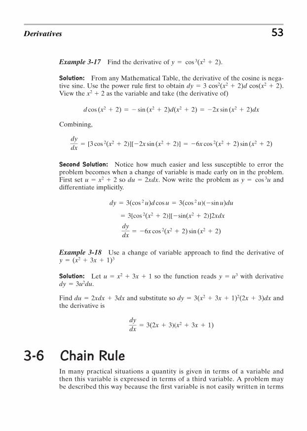
Example 3-17 Find the derivative of .
Solution: From any Mathematical Table, the derivative of the cosine is nega-tive sine. Use the power rule first to obtain dy 3 cos2(x2 2)d cos(x2 2).View the x2 2 as the variable and take (the derivative of)
Combining,
Second Solution: Notice how much easier and less susceptible to error theproblem becomes when a change of variable is made early on in the problem.First set so . Now write the problem as anddifferentiate implicitly.
Example 3-18 Use a change of variable approach to find the derivative of
Solution: Let so the function reads with derivative.
Find and substitute so andthe derivative is
3-6 Chain RuleIn many practical situations a quantity is given in terms of a variable andthen this variable is expressed in terms of a third variable. A problem maybe described this way because the first variable is not easily written in terms
dydx
3(2x 3)(x2 3x 1)
dy 3(x2 3x 1)2(2x 3)dxdu 2xdx 3dx
dy 3u2duy u3u x2 3x 1
y (x2 3x 1)3
dydx
6x cos 2(x2 2) sin (x2 2)
3[cos 2(x2 2)][sin(x2 2)]2xdx
dy 3(cos 2 u)d cos u 3(cos 2 u)(sin u)du
y cos 3udu 2xdxu x2 2
dydx
[3 cos 2(x2 2)][2x sin (x2 2)] 6x cos 2(x2 2) sin (x2 2)
d cos (x2 2) sin (x2 2)d(x2 2) 2x sin (x2 2)dx
y cos 3(x2 2)
Derivatives 53

of the third or perhaps it is conceptually easier to understand the process intwo steps.
54 CALCULUS FOR THE UTTERLY CONFUSED
Suppose the cost of manufacturing a certain item, say a computer chip, dependson the number of items produced. The number of items produced depends onthe length of time the “fab” facility operates to produce the chips, the length oftime for the production run. If the cost per unit (dollars per chip) is andthe rate of production (chips per hour) is , then cost per unit of time is theproduct of these two derivatives.
Example 3-19 Find du/dt for and .
Solution: This requires a chain derivative:
Example 3-20 The monthly profit for selling tacos follows:
where q is the number of tacos sold. The relation between number of workersand tacos is .
Find dP/dn, the profit per worker for q 1000 tacos sold.
Solution: This problem requires a chain derivative: .
dPdq
30 0.004q anddqdn
100
dPdn
dPdq
dqdn
q 100n
P 1200 30q 0.002q2
dudt
dudx
dxdt
(2x 2)(3t 2)
dudt
dudx
dxdt
x t 3 3u x2 2x
dCdt
dCdN
dNdt
dN/dtdC/dN
Sandprecious metals
Chip Factory Chips
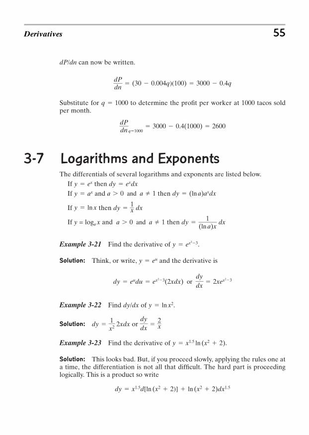
dP/dn can now be written.
Substitute for q 1000 to determine the profit per worker at 1000 tacos soldper month.
3-7 Logarithms and ExponentsThe differentials of several logarithms and exponents are listed below.
If then If and then
If then
If y = loga x and then
Example 3-21 Find the derivative of .
Solution: Think, or write, and the derivative is
Example 3-22 Find of .
Solution: or
Example 3-23 Find the derivative of .
Solution: This looks bad. But, if you proceed slowly, applying the rules one ata time, the differentiation is not all that difficult. The hard part is proceedinglogically. This is a product so write
dy x1.5d[ln (x2 2)] ln (x2 2)dx1.5
y x1.5 ln (x2 2)
dydx
2xdy
1x2 2xdx
y ln x2dy/dx
dy eudu ex23(2xdx) ordydx
2xex23
y eu
y ex23
dy 1
(ln a)xdxa 0 and a 2 1
dy 1x dxy ln x
dy (ln a)axdxa 0 and a 2 1y ax
dy exdxy ex
dPdn q1000
3000 0.4(1000) 2600
dPdn
(30 0.004q)(100) 3000 0.4q
Derivatives 55
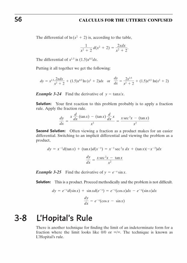
The differential of is, according to the table,
.
The differential of is .
Putting it all together we get the following:
Example 3-24 Find the derivative of y tanx/x.
Solution: Your first reaction to this problem probably is to apply a fractionrule. Apply the fraction rule.
Second Solution: Often viewing a fraction as a product makes for an easierdifferential. Switching to an implicit differential and viewing the problem as aproduct,
Example 3-25 Find the derivative of .
Solution: This is a product. Proceed methodically and the problem is not difficult.
3-8 L’Hopital’s RuleThere is another technique for finding the limit of an indeterminate form for afraction where the limit looks like 0/0 or /. The technique is known asL’Hopital’s rule.
dydx
ex(cos x sin x)
dy exd(sin x) sin xd(ex) ex(cos x)dx ex(sin x)dx
y ex sin x
dydx
x sec 2x tan x
x2
dy x1d(tan x) (tan x)d(x1) x1 sec 2x dx (tan x)(x2)dx
dydx
x d
dx (tan x) (tan x) d
dxx
x2 x sec 2x (tan x)
x2
dy x1.5 2xdxx2 2
(1.5)x0.5 In (x2 2)dx or dydx
2x2.5
x2 2 (1.5)x0.5 In(x2 2)
(1.5)x0.5dxx1.5
1x2 2
d(x2 2) 2xdx
x2 2
ln (x2 2)
56 CALCULUS FOR THE UTTERLY CONFUSED
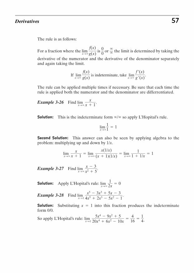
The rule is as follows:
For a fraction where the is or the limit is determined by taking the
derivative of the numerator and the derivative of the denominator separatelyand again taking the limit.
The rule can be applied multiple times if necessary. Be sure that each time therule is applied both the numerator and the denominator are differrentiated.
Example 3-26 Find .
Solution: This is the indeterminate form so apply L’Hopital’s rule.
Second Solution: This answer can also be seen by applying algebra to theproblem: multiplying up and down by 1/x.
Example 3-27 Find .
Solution: Apply L’Hopital’s rule:
Example 3-28 Find .
Solution: Substituting x 1 into this fraction produces the indeterminateform 0/0.
So apply L’Hopital’s rule: .limxS1
5x4 9x2 520x4 6x2 10x
416
14
limxS1
x5 3x3 5x 34x5 2x3 5x2 1
limxS`
12x
0
limxS`
x 3x2 5
limxS`
xx 1
limxS`
x(1/x)(x 1)(1/x)
limxS`
11 1/x
1
limxS`
11 1
`/`
limxS`
xx 1
If limxS`
f(x)g(x)
is indeterminate, take limxS`
f r(x)g r(x)
.
``
00lim
xS`
f(x)g(x)
Derivatives 57
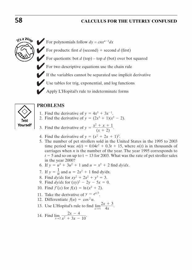
For polynomials follow dy = cnxn1dx
For products: first d (second) second d (first)
For quotients: bot d (top) – top d (bot) over bot squared
For two descriptive equations use the chain rule
If the variables cannot be separated use implicit derivative
Use tables for trig, exponential, and log functions
Apply L’Hopital’s rule to indeterminate forms
PROBLEMS
1. Find the derivative of .2. Find the derivative of .
3. Find the derivative of .
4. Find the derivative of .5. The number of pet strollers sold in the United States in the 1995 to 2003
time period was: , where n(t) is in thousands ofcarriages when n is the number of the year. The year 1995 corresponds tot 5 and so on up to t 13 for 2003. What was the rate of pet stroller salesin the year 2000?
6. If and find dy/dx.
7. If and find dy/dx. 8. Find dy/dx for .9. Find dy/dx for .
10. Find for .
11. Take the derivative of .12. Differentiate .
13. Use L’Hopital’s rule to find .
14. Find .limxS2
2x 4x2 3x 10
limxS`
2x 34x
f(u) cos 2 uy ex>3
f(x) ln (x2 2)f r(x)(xy)2 2y 5x 0xy2 2x2 y3 3
u 2x2 1y 1u
u x2 2y u3 3u2 1
n(t) 0.04t 2 0.3t 15
y (x2 2x 1)3
y x2 x 1
(x 2)
y (2x3 1)(x2 2)y 4x3 3x1
58 CALCULUS FOR THE UTTERLY CONFUSED
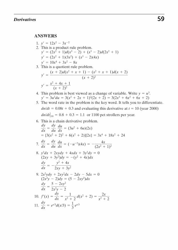
ANSWERS
1.2. This is a product rule problem.
3. This is a quotient rule problem.
4. This problem is best viewed as a change of variable. Write .
5. The word rate in the problem is the key word. It tells you to differentiate.
and evaluating this derivative at t 10 (year 2000)
or 1100 pet strollers per year.
6. This is a chain derivative problem.
7.
8.
9.
10.
11.dydx
ex/3d(x/3) 13 ex/3
f r(x) dydx
1
x2 2d(x2 2)
2xx2 2
dydx
5 2xy2
2x2y 2
(2x2y 2)dy (5 2xy2)dx2x2ydy 2xy2dx 2dy 5dx 0
dydx
y2 4x
2xy 3y2
(2xy 3y2)dy (y2 4x)dxy2dx 2xydy 4xdx 3y2dy 0
dydx
dydu
dudx
(u2)(4x) 4x
(2x2 1)2
[3(x2 2)2 6(x2 2)][2x] 3x4 18x2 24
dydx
dydu
dudx
(3u2 6u)(2x)
dn/dtZ10 0.8 0.3 1.1
dn/dt 0.08t 0.3
yr 3u2du 3(x2 2x 1)2(2x 2) 3(2x3 6x2 6x 2)y u3
yr x2 4x 1
(x 2)2
yr (x 2)d(x2 x 1) (x2 x 1)d(x 2)
(x 2)2
yr 10x4 3x2 8xyr (2x2 1)(3x2) (x3 2)(4x)yr (2x2 1)d(x3 2) (x3 2)d(2x2 1)
yr 12x2 3x2
Derivatives 59
12.
13.
14. This is an indeterminate form for x 2, so use L’Hopital’s rule.
limxS2
22x 3
27
lim xS`
24
12
f r(u) 2(cos u)d(cos u) 2(sin u)(cos u)
60 CALCULUS FOR THE UTTERLY CONFUSED

CHAPTER 4
GRAPHING
You should read this chapter if you need to review or you need to learn about
Graphing cubic and higher power curves
Finding max and min points of graphs
Identifying points of inflection
Interpreting graphs of real problems
61
Copyright © 2007 by The McGraw-Hill Companies, Inc. Click here for terms of use.
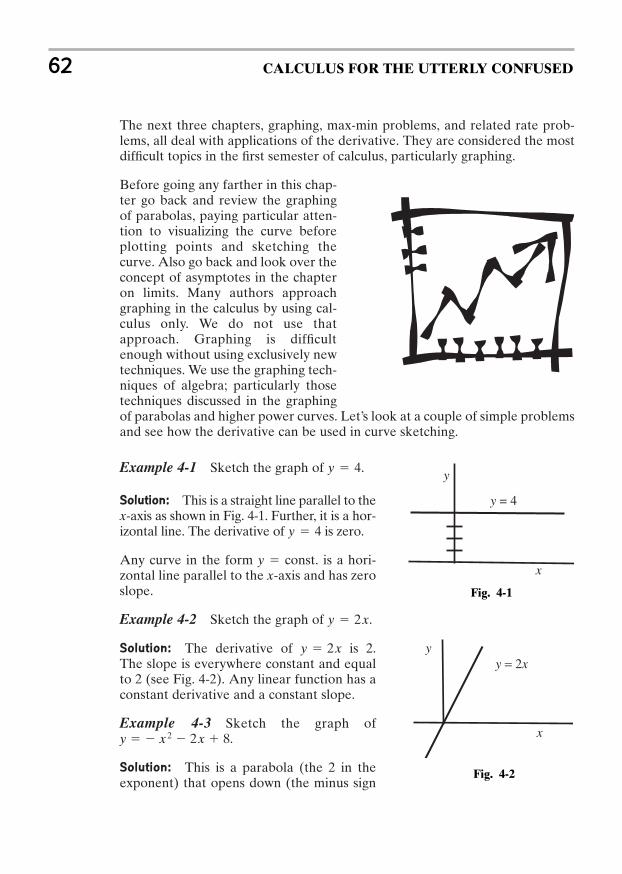
The next three chapters, graphing, max-min problems, and related rate prob-lems, all deal with applications of the derivative. They are considered the mostdifficult topics in the first semester of calculus, particularly graphing.
Before going any farther in this chap-ter go back and review the graphingof parabolas, paying particular atten-tion to visualizing the curve beforeplotting points and sketching thecurve. Also go back and look over theconcept of asymptotes in the chapteron limits. Many authors approachgraphing in the calculus by using cal-culus only. We do not use thatapproach. Graphing is difficultenough without using exclusively newtechniques. We use the graphing tech-niques of algebra; particularly thosetechniques discussed in the graphingof parabolas and higher power curves. Let’s look at a couple of simple problemsand see how the derivative can be used in curve sketching.
Example 4-1 Sketch the graph of .
Solution: This is a straight line parallel to thex-axis as shown in Fig. 4-1. Further, it is a hor-izontal line. The derivative of is zero.
Any curve in the form y const. is a hori-zontal line parallel to the x-axis and has zeroslope.
Example 4-2 Sketch the graph of .
Solution: The derivative of is 2.The slope is everywhere constant and equalto 2 (see Fig. 4-2). Any linear function has aconstant derivative and a constant slope.
Example 4-3 Sketch the graph of y x 2 2x 8.
Solution: This is a parabola (the 2 in theexponent) that opens down (the minus sign
y 2x
y 2x
y 4
y 4
62 CALCULUS FOR THE UTTERLY CONFUSED
Fig. 4-1
y
x
y = 4
Fig. 4-2
x
yy = 2x
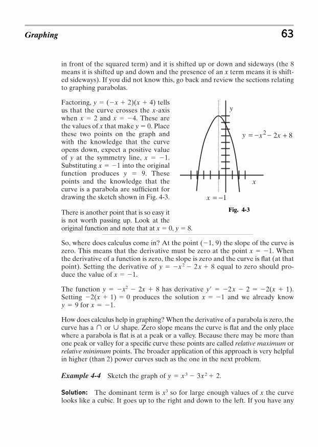
in front of the squared term) and it is shifted up or down and sideways (the 8means it is shifted up and down and the presence of an x term means it is shift-ed sideways). If you did not know this, go back and review the sections relatingto graphing parabolas.
Factoring, y (x 2)(x 4) tellsus that the curve crosses the x-axiswhen x 2 and x 4. These arethe values of x that make y 0. Placethese two points on the graph andwith the knowledge that the curveopens down, expect a positive valueof y at the symmetry line, x 1.Substituting x 1 into the originalfunction produces y 9. Thesepoints and the knowledge that thecurve is a parabola are sufficient fordrawing the sketch shown in Fig. 4-3.
There is another point that is so easy itis not worth passing up. Look at theoriginal function and note that at x 0, y 8.
So, where does calculus come in? At the point (1, 9) the slope of the curve iszero. This means that the derivative must be zero at the point x 1. Whenthe derivative of a function is zero, the slope is zero and the curve is flat (at thatpoint). Setting the derivative of equal to zero should pro-duce the value of x 1.
The function y x2 2x 8 has derivative y 2x 2 2(x 1).Setting produces the solution and we already know
for .
How does calculus help in graphing? When the derivative of a parabola is zero, thecurve has a or shape. Zero slope means the curve is flat and the only placewhere a parabola is flat is at a peak or a valley. Because there may be more thanone peak or valley for a specific curve these points are called relative maximum orrelative minimum points. The broader application of this approach is very helpfulin higher (than 2) power curves such as the one in the next problem.
Example 4-4 Sketch the graph of .
Solution: The dominant term is so for large enough values of x the curvelooks like a cubic. It goes up to the right and down to the left. If you have any
x3
y x 3 3x 2 2
´¨
x 1y 9x 12(x 1) 0
y x 2 2x 8
Graphing 63
Fig. 4-3
y
x
= −1x
2x2 + 8= xy __
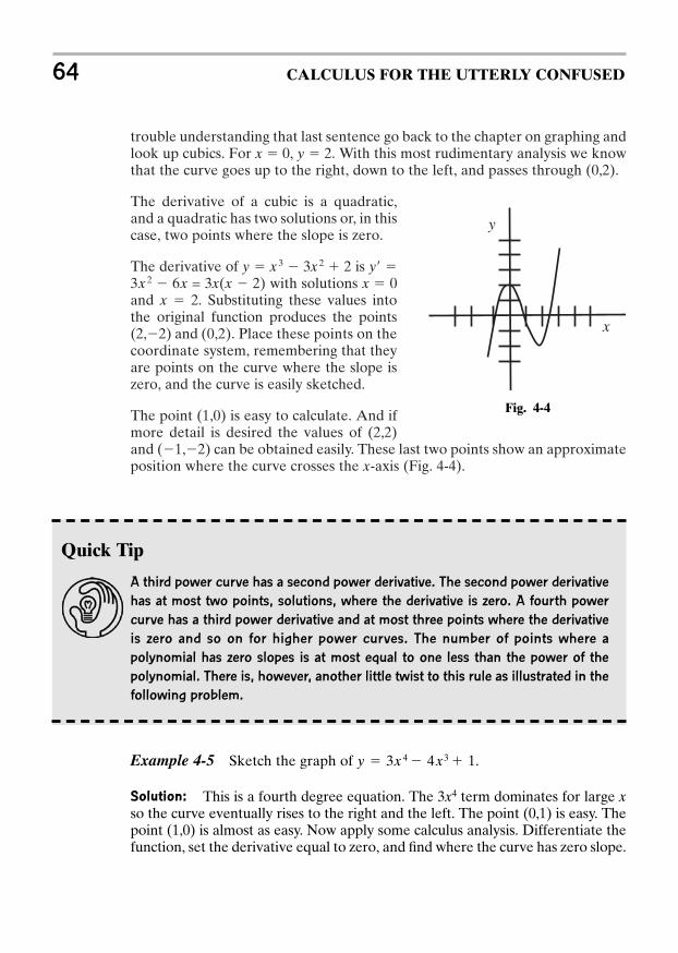
trouble understanding that last sentence go back to the chapter on graphing andlook up cubics. For x 0, y 2. With this most rudimentary analysis we knowthat the curve goes up to the right, down to the left, and passes through (0,2).
The derivative of a cubic is a quadratic,and a quadratic has two solutions or, in thiscase, two points where the slope is zero.
The derivative of y x3 3x2 2 is y 3x 2 6x = 3x(x 2) with solutions x 0and x 2. Substituting these values intothe original function produces the points(2,2) and (0,2). Place these points on thecoordinate system, remembering that theyare points on the curve where the slope iszero, and the curve is easily sketched.
The point (1,0) is easy to calculate. And ifmore detail is desired the values of (2,2)and (1,2) can be obtained easily. These last two points show an approximateposition where the curve crosses the x-axis (Fig. 4-4).
64 CALCULUS FOR THE UTTERLY CONFUSED
Quick Tip
A third power curve has a second power derivative. The second power derivative
has at most two points, solutions, where the derivative is zero. A fourth power
curve has a third power derivative and at most three points where the derivative
is zero and so on for higher power curves. The number of points where a
polynomial has zero slopes is at most equal to one less than the power of the
polynomial. There is, however, another little twist to this rule as illustrated in the
following problem.
Example 4-5 Sketch the graph of .
Solution: This is a fourth degree equation. The term dominates for large xso the curve eventually rises to the right and the left. The point (0,1) is easy. Thepoint (1,0) is almost as easy. Now apply some calculus analysis. Differentiate thefunction, set the derivative equal to zero, and find where the curve has zero slope.
3x4
y 3x 4 4x3 1
y
x
Fig. 4-4
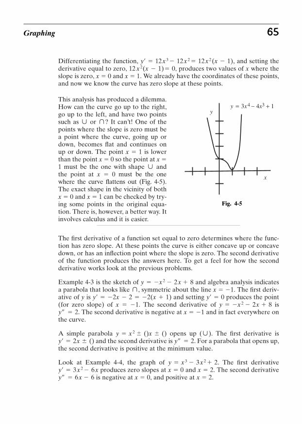
Differentiating the function, , and setting thederivative equal to zero, , produces two values of x where theslope is zero, x 0 and x 1. We already have the coordinates of these points,and now we know the curve has zero slope at these points.
This analysis has produced a dilemma.How can the curve go up to the right,go up to the left, and have two pointssuch as or ? It can’t! One of thepoints where the slope is zero must bea point where the curve, going up ordown, becomes flat and continues onup or down. The point x 1 is lowerthan the point x 0 so the point at x 1 must be the one with shape andthe point at x 0 must be the onewhere the curve flattens out (Fig. 4-5).The exact shape in the vicinity of bothx 0 and x 1 can be checked by try-ing some points in the original equa-tion. There is, however, a better way. Itinvolves calculus and it is easier.
The first derivative of a function set equal to zero determines where the func-tion has zero slope. At these points the curve is either concave up or concavedown, or has an inflection point where the slope is zero. The second derivativeof the function produces the answers here. To get a feel for how the secondderivative works look at the previous problems.
Example 4-3 is the sketch of and algebra analysis indicatesa parabola that looks like , symmetric about the line x 1. The first deriv-ative of y is and setting produces the point(for zero slope) of x 1. The second derivative of is
. The second derivative is negative at x 1 and in fact everywhere onthe curve.
A simple parabola opens up ( ). The first derivative isand the second derivative is . For a parabola that opens up,
the second derivative is positive at the minimum value.
Look at Example 4-4, the graph of . The first derivativeproduces zero slopes at x 0 and x 2. The second derivative
is negative at x 0, and positive at x 2.yrr 6x 6yr 3x 2 6x
y x 3 3x 2 2
yrr 2yr 2x ()´y x 2 ()x ()
yrr 2y x 2 2x 8
yr 0yr 2x 2 2(x 1)¨
y x 2 2x 8
´
¨´
12 x 2(x 1) 0yr 12x 3 12x 2 12x 2(x 1)
Graphing 65
Fig. 4-5
4x3 + 13x4 _=yy
x
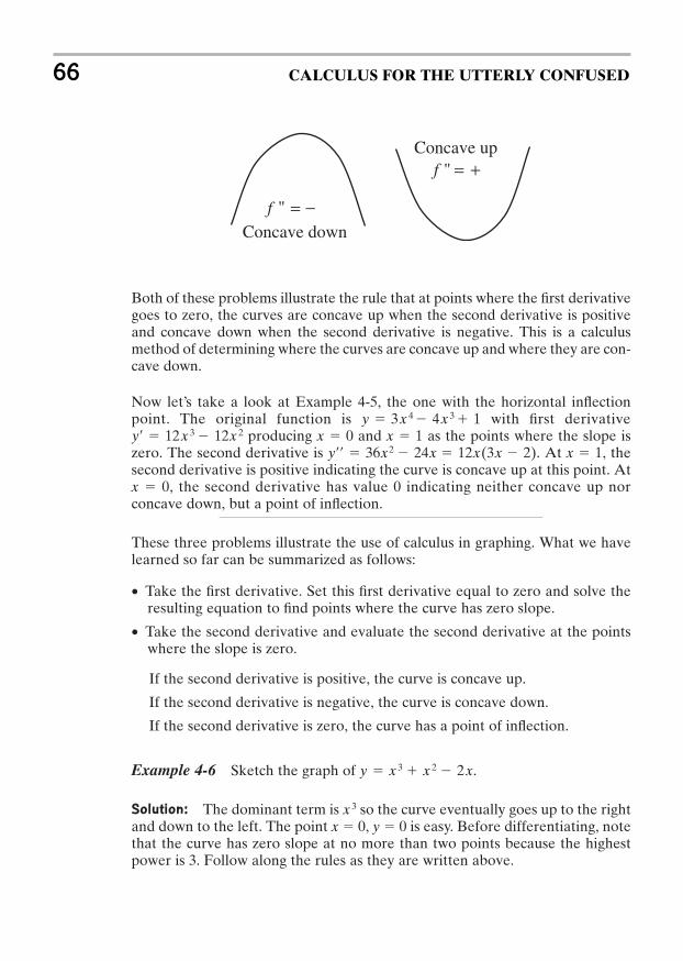
Both of these problems illustrate the rule that at points where the first derivativegoes to zero, the curves are concave up when the second derivative is positiveand concave down when the second derivative is negative. This is a calculusmethod of determining where the curves are concave up and where they are con-cave down.
Now let’s take a look at Example 4-5, the one with the horizontal inflectionpoint. The original function is with first derivative
producing x 0 and x 1 as the points where the slope iszero. The second derivative is . At x 1, thesecond derivative is positive indicating the curve is concave up at this point. Atx 0, the second derivative has value 0 indicating neither concave up norconcave down, but a point of inflection.
These three problems illustrate the use of calculus in graphing. What we havelearned so far can be summarized as follows:
• Take the first derivative. Set this first derivative equal to zero and solve theresulting equation to find points where the curve has zero slope.
• Take the second derivative and evaluate the second derivative at the pointswhere the slope is zero.
If the second derivative is positive, the curve is concave up.
If the second derivative is negative, the curve is concave down.
If the second derivative is zero, the curve has a point of inflection.
Example 4-6 Sketch the graph of .
Solution: The dominant term is so the curve eventually goes up to the rightand down to the left. The point x 0, y 0 is easy. Before differentiating, notethat the curve has zero slope at no more than two points because the highestpower is 3. Follow along the rules as they are written above.
x 3
y x 3 x 2 2x
yrr 36x2 24x 12x(3x 2)yr 12x 3 12x 2
y 3x 4 4x 3 1
66 CALCULUS FOR THE UTTERLY CONFUSED
Concave up +
−
="
"
f
=fConcave down
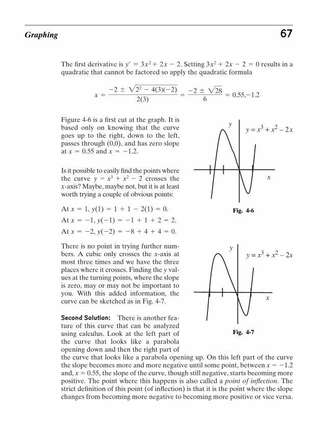
The first derivative is . Setting results in aquadratic that cannot be factored so apply the quadratic formula
Figure 4-6 is a first cut at the graph. It isbased only on knowing that the curvegoes up to the right, down to the left,passes through (0,0), and has zero slopeat and .
Is it possible to easily find the points wherethe curve crosses thex-axis? Maybe, maybe not, but it is at leastworth trying a couple of obvious points:
At , .
At , .
At , .
There is no point in trying further num-bers. A cubic only crosses the x-axis atmost three times and we have the threeplaces where it crosses. Finding the y val-ues at the turning points, where the slopeis zero, may or may not be important toyou. With this added information, thecurve can be sketched as in Fig. 4-7.
Second Solution: There is another fea-ture of this curve that can be analyzedusing calculus. Look at the left part ofthe curve that looks like a parabolaopening down and then the right part ofthe curve that looks like a parabola opening up. On this left part of the curvethe slope becomes more and more negative until some point, between x 1.2and, x 0.55, the slope of the curve, though still negative, starts becoming morepositive. The point where this happens is also called a point of inflection. Thestrict definition of this point (of inflection) is that it is the point where the slopechanges from becoming more negative to becoming more positive or vice versa.
y(2) 8 4 4 0x 2
y(1) 1 1 2 2x 1
y(1) 1 1 2(1) 0x 1
y x3 x2 2
x 1.2x 0.55
x 2 222 4(3)(2)
2(3)
2 2286
0.55,1.2
3x2 2x 2 0yr 3x 2 2x 2
Graphing 67
Fig. 4-6
y = x3 + x2 – 2xy
x
Fig. 4-7
y
x
y = x3 + x2 – 2x
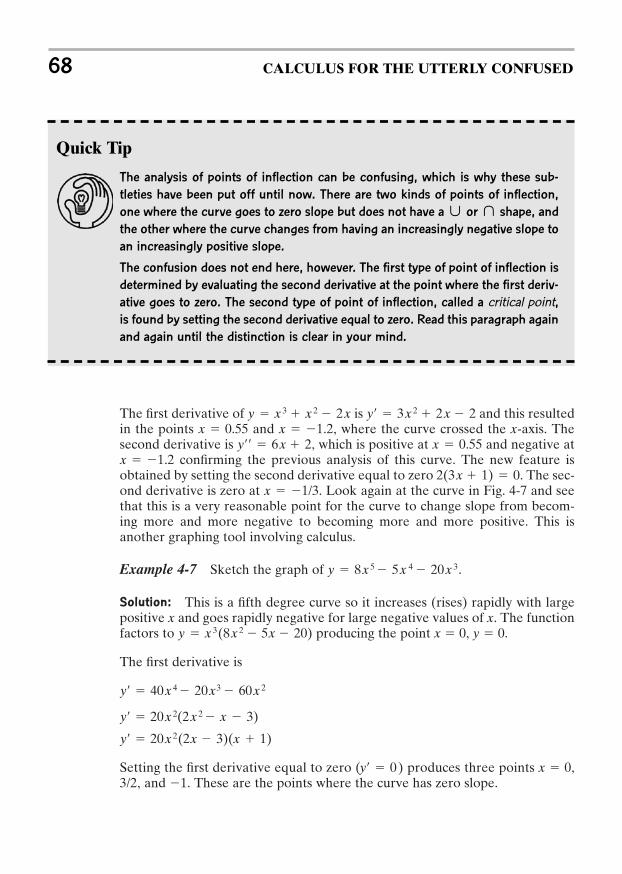
The first derivative of is and this resultedin the points and , where the curve crossed the x-axis. Thesecond derivative is , which is positive at and negative at
confirming the previous analysis of this curve. The new feature isobtained by setting the second derivative equal to zero . The sec-ond derivative is zero at . Look again at the curve in Fig. 4-7 and seethat this is a very reasonable point for the curve to change slope from becom-ing more and more negative to becoming more and more positive. This isanother graphing tool involving calculus.
Example 4-7 Sketch the graph of .
Solution: This is a fifth degree curve so it increases (rises) rapidly with largepositive x and goes rapidly negative for large negative values of x. The functionfactors to producing the point x 0, y 0.
The first derivative is
Setting the first derivative equal to zero ( ) produces three points x 0,3/2, and 1. These are the points where the curve has zero slope.
yr 0
yr 20x 2(2x 3)(x 1)
yr 20x 2(2x 2 x 3)
yr 40x 4 20x3 60x 2
y x 3(8x 2 5x 20)
y 8x 5 5x 4 20x 3
x 1/32(3x 1) 0
x 1.2x 0.55yrr 6x 2
x 1.2x 0.55yr 3x 2 2x 2y x 3 x 2 2x
68 CALCULUS FOR THE UTTERLY CONFUSED
Quick Tip
The analysis of points of inflection can be confusing, which is why these sub-
tleties have been put off until now. There are two kinds of points of inflection,
one where the curve goes to zero slope but does not have a or shape, and
the other where the curve changes from having an increasingly negative slope to
an increasingly positive slope.
The confusion does not end here, however. The first type of point of inflection is
determined by evaluating the second derivative at the point where the first deriv-
ative goes to zero. The second type of point of inflection, called a critical point,is found by setting the second derivative equal to zero. Read this paragraph again
and again until the distinction is clear in your mind.
¨´
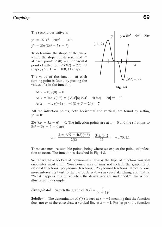
The second derivative is
To determine the shape of the curvewhere the slope equals zero, find yat each point: , horizontalpoint of inflection; , shape; , shape.
The value of the function at eachturning point is found by putting thevalues of x in the function.
At ,
At ,
At ,
All the inflection points, both horizontal and vertical, are found by setting:
. The inflection points are at and the solutions toare
These are most reasonable points, being where we expect the points of inflec-tion to occur. The function is sketched in Fig. 4-8.
So far we have looked at polynomials. This is the type of function you willencounter most often. Your course may or may not include the graphing ofrational functions (polynomial fractions). Polynomial fractions introduce onemore interesting twist to the use of derivatives in curve sketching, and that is:“What happens to a curve when the derivatives are undefined.” This is bestillustrated by example.
Example 4-8 Sketch the graph of .
Solution: The denominator of is zero at x 1 meaning that the functiondoes not exist there, so draw a vertical line at x 1. For large x, the function
f(x)
f(x) x
(x 1)2
x 3 29 4(8)(6)
2(8)
3 14.216
0.70, 1.1
8x2 3x 6 0x 020x(8x2 3x 6) 0
yrr 0
y(1) 1(8 5 20) 7x 1
y(3/2) (3/2)3[8(3/2)2 5(3/2) 20] < 32x 3/2
y(0) 0x 0
¨yrr (1) 100´yrr (3/2) 225
yrr (0) 0
yrr 20x(8x2 3x 6)
yrr 160x3 60x2 120x
Graphing 69
Fig. 4-8
(3/2, _32)
(_1, 7)
y
x
y = 8x5 – 5x4 – 20x
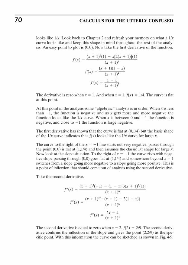
looks like 1/x. Look back to Chapter 2 and refresh your memory on what a 1/xcurve looks like and keep this shape in mind throughout the rest of the analy-sis. An easy point to plot is (0,0). Now take the first derivative of the function.
The derivative is zero when x 1. And when x 1, . The curve is flatat this point.
At this point in the analysis some “algebraic” analysis is in order. When x is lessthan 1, the function is negative and as x gets more and more negative thefunction looks like the 1/x curve. When x is between 0 and 1 the function isnegative, and close to 1 the function is large negative.
The first derivative has shown that the curve is flat at (0,1/4) but the basic shapeof the 1/x curve indicates that looks like the 1/x curve for large x.
The curve to the right of the x 1 line starts out very negative, passes throughthe point (0,0) is flat at (1,1/4) and then assumes the classic 1/x shape for large x.Now look at the slope situation. To the right of x 1 the curve rises with nega-tive slope passing through (0,0) goes flat at (1,1/4) and somewhere beyond x 1switches from a slope going more negative to a slope going more positive. This isa point of inflection that should come out of analysis using the second derivative.
Take the second derivative.
The second derivative is equal to zero when x 2. . The second deriv-ative confirms the inflection in the slope and gives the point (2,2/9) as the spe-cific point. With this information the curve can be sketched as shown in Fig. 4-9.
f(2) 2/9
f rr(x) 2x 4
(x 1)4
f rr(x) (x 1)2[(x 1) 3(1 x)]
(x 1)6
f rr(x) (x 1)3(1) (1 x)[3(x 1)2(1)]
(x 1)6
f(x)
f(x) 1/4
f r(x) 1 x
(x 1)3
f r(x) (x 1)(1 x)
(x 1)4
f r(x) (x 1)2(1) x[2(x 1)](1)
(x 1)4
70 CALCULUS FOR THE UTTERLY CONFUSED
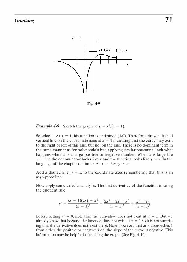
Example 4-9 Sketch the graph of .
Solution: At this function is undefined ( ). Therefore, draw a dashedvertical line on the coordinate axes at indicating that the curve may existto the right or left of this line, but not on the line. There is no dominant term inthe same manner as for polynomials but, applying similar reasoning, look whathappens when x is a large positive or negative number. When x is large the
in the denominator looks like x and the function looks like . In thelanguage of the chapter on limits: As , .
Add a dashed line, , to the coordinate axes remembering that this is anasymptote line.
Now apply some calculus analysis. The first derivative of the function is, usingthe quotient rule:
Before setting , note that the derivative does not exist at . But wealready knew that because the function does not exist at so it is not surpris-ing that the derivative does not exist there. Note, however, that as x approaches 1from either the positive or negative side, the slope of the curve is negative. Thisinformation may be helpful in sketching the graph. (See Fig. 4-10.)
x 1x 1yr 0
yr (x 1)(2x) x 2
(x 1)2 2x2 2x x 2
(x 1)2 x 2 2x(x 1)2
y x
y < xx S `y < xx 1
x 11/0x 1
y x 2/(x 1)
Graphing 71
Fig. 4-9
Setting produces , and the two points where the slope equalszero are and . The values of the function for these two points are: y(0) 0 and so the slope of the curve is zero at (0,0) and (2,4).
If you are unsure of the shape of the curve in certain regions, check a point.With the information generated from the calculus and the concepts of limits youshould get very close to the correct curve. As you gain more confidence you willnot resort to checking specific areas of the curve by testing a point.
The previous problem is typical of the more difficult ones you will encounter inyour course. It is probably beyond what you will encounter on a test because of thecomplexity of the analysis and the potential for confusion. Sketches of the graphsof polynomials are much more popular as test problems. Know how to graph poly-nomials and you will be well along toward a good test score in graphing.
Having gone through examples of what you can expect to encounter in graph-ing problems, it is now time to write down some procedural guidelines forgraphing curves of the general form .
Guidelines for Graphing with Calculus1. Look for the dominant term. If the function is a polynomial, the highest-
power term gives the shape of the curve for large positive or negative numbers
y f(x)
y(2) 22/(2 1) 4x 2x 0
x(x 2) 0yr 0
72 CALCULUS FOR THE UTTERLY CONFUSED
Fig. 4-10
y
x
=x – 1
x2y
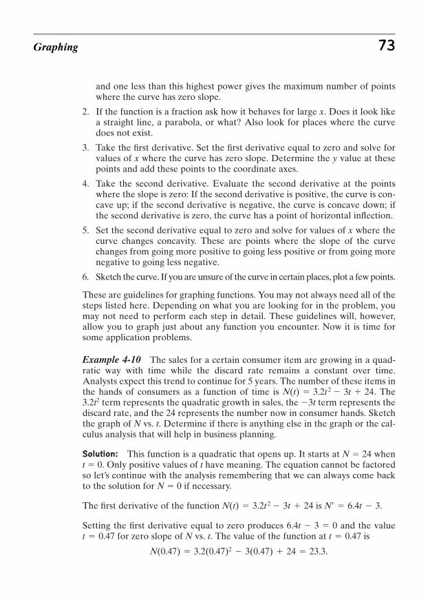
and one less than this highest power gives the maximum number of pointswhere the curve has zero slope.
2. If the function is a fraction ask how it behaves for large x. Does it look likea straight line, a parabola, or what? Also look for places where the curvedoes not exist.
3. Take the first derivative. Set the first derivative equal to zero and solve forvalues of x where the curve has zero slope. Determine the y value at thesepoints and add these points to the coordinate axes.
4. Take the second derivative. Evaluate the second derivative at the pointswhere the slope is zero: If the second derivative is positive, the curve is con-cave up; if the second derivative is negative, the curve is concave down; ifthe second derivative is zero, the curve has a point of horizontal inflection.
5. Set the second derivative equal to zero and solve for values of x where thecurve changes concavity. These are points where the slope of the curvechanges from going more positive to going less positive or from going morenegative to going less negative.
6. Sketch the curve. If you are unsure of the curve in certain places, plot a few points.
These are guidelines for graphing functions. You may not always need all of thesteps listed here. Depending on what you are looking for in the problem, youmay not need to perform each step in detail. These guidelines will, however,allow you to graph just about any function you encounter. Now it is time forsome application problems.
Example 4-10 The sales for a certain consumer item are growing in a quad-ratic way with time while the discard rate remains a constant over time.Analysts expect this trend to continue for 5 years. The number of these items inthe hands of consumers as a function of time is . The3.2t2 term represents the quadratic growth in sales, the 3t term represents thediscard rate, and the 24 represents the number now in consumer hands. Sketchthe graph of N vs. t. Determine if there is anything else in the graph or the cal-culus analysis that will help in business planning.
Solution: This function is a quadratic that opens up. It starts at N 24 whent 0. Only positive values of t have meaning. The equation cannot be factoredso let’s continue with the analysis remembering that we can always come backto the solution for N 0 if necessary.
The first derivative of the function is .
Setting the first derivative equal to zero produces and the valuefor zero slope of N vs. t. The value of the function at is
.N(0.47) 3.2(0.47)2 3(0.47) 24 23.3
t 0.47t 0.476.4t 3 0
Nr 6.4t 3N(t) 3.2t 2 3t 24
N(t) 3.2t 2 3t 24
Graphing 73
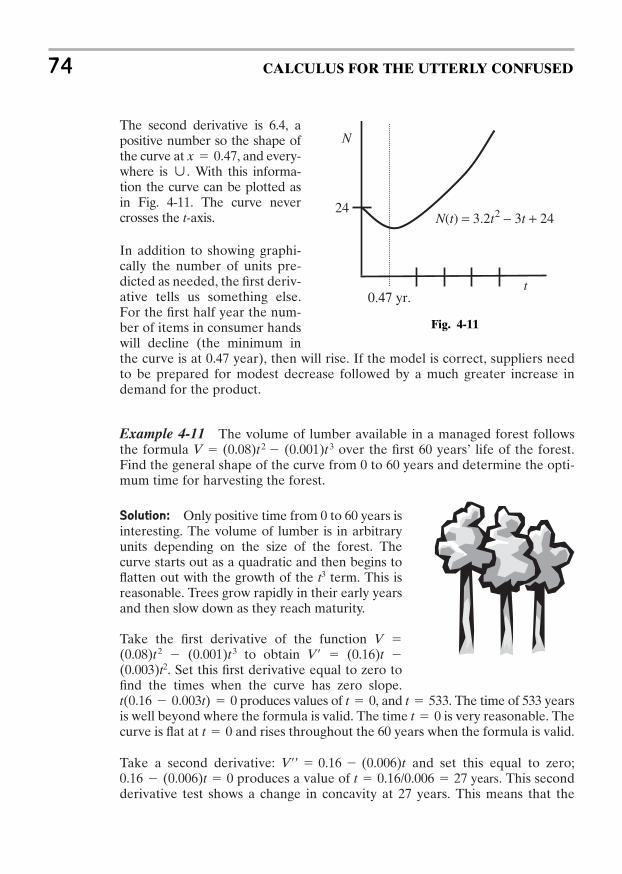
The second derivative is 6.4, apositive number so the shape ofthe curve at , and every-where is . With this informa-tion the curve can be plotted asin Fig. 4-11. The curve nevercrosses the t-axis.
In addition to showing graphi-cally the number of units pre-dicted as needed, the first deriv-ative tells us something else.For the first half year the num-ber of items in consumer handswill decline (the minimum inthe curve is at 0.47 year), then will rise. If the model is correct, suppliers needto be prepared for modest decrease followed by a much greater increase indemand for the product.
Example 4-11 The volume of lumber available in a managed forest followsthe formula over the first 60 years’ life of the forest.Find the general shape of the curve from 0 to 60 years and determine the opti-mum time for harvesting the forest.
Solution: Only positive time from 0 to 60 years isinteresting. The volume of lumber is in arbitraryunits depending on the size of the forest. Thecurve starts out as a quadratic and then begins toflatten out with the growth of the t3 term. This isreasonable. Trees grow rapidly in their early yearsand then slow down as they reach maturity.
Take the first derivative of the function V (0.08)t2 (0.001)t3 to obtain V (0.16)t (0.003)t2. Set this first derivative equal to zero tofind the times when the curve has zero slope.
produces values of , and . The time of 533 yearsis well beyond where the formula is valid. The time is very reasonable. Thecurve is flat at and rises throughout the 60 years when the formula is valid.
Take a second derivative: and set this equal to zero;produces a value of . This second
derivative test shows a change in concavity at 27 years. This means that thet 0.16/0.006 27 years0.16 (0.006)t 0
Vrr 0.16 (0.006)t
t 0t 0
t 533t 0t(0.16 0.003t) 0
V (0.08)t 2 (0.001)t 3
´x 0.47
74 CALCULUS FOR THE UTTERLY CONFUSED
Fig. 4-11
24N(t) = 3.2t2 − 3t + 24
0.47 yr.
N
t
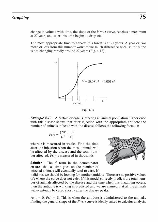
change in volume with time, the slope of the V vs. t curve, reaches a maximumat 27 years and after this time begins to drop off.
The most appropriate time to harvest this forest is at 27 years. A year or twomore or less from this number won’t make much difference because the slopeis not changing rapidly around 27 years (Fig. 4-12).
Graphing 75
Fig. 4-12
V = (0.08)t2 _ (0.001)t3
27 yrs.t
V
Example 4-12 A certain disease is infecting an animal population. Experiencewith this disease shows that after injection with the appropriate antidote thenumber of animals infected with the disease follows the following formula:
where t is measured in weeks. Find the timeafter the injection when the most animals willbe affected by the disease and the total num-ber affected. P(t) is measured in thousands.
Solution: The t2 term in the denominatorensures that as time goes on the number ofinfected animals will eventually tend to zero. Ifit did not, we should be looking for another antidote! There are no positive valuesof t where the curve does not exist. If this model correctly predicts the total num-ber of animals affected by the disease and the time when this maximum occurs,then the antidote is working as predicted and we are assured that all the animalswill eventually be cured shortly after the disease peaks.
At t 0, P(t) 8. This is when the antidote is administered to the animals.Finding the general shape of the P vs. t curve is ideally suited to calculus analysis.
P(t) (20t 8)(t 2 1)
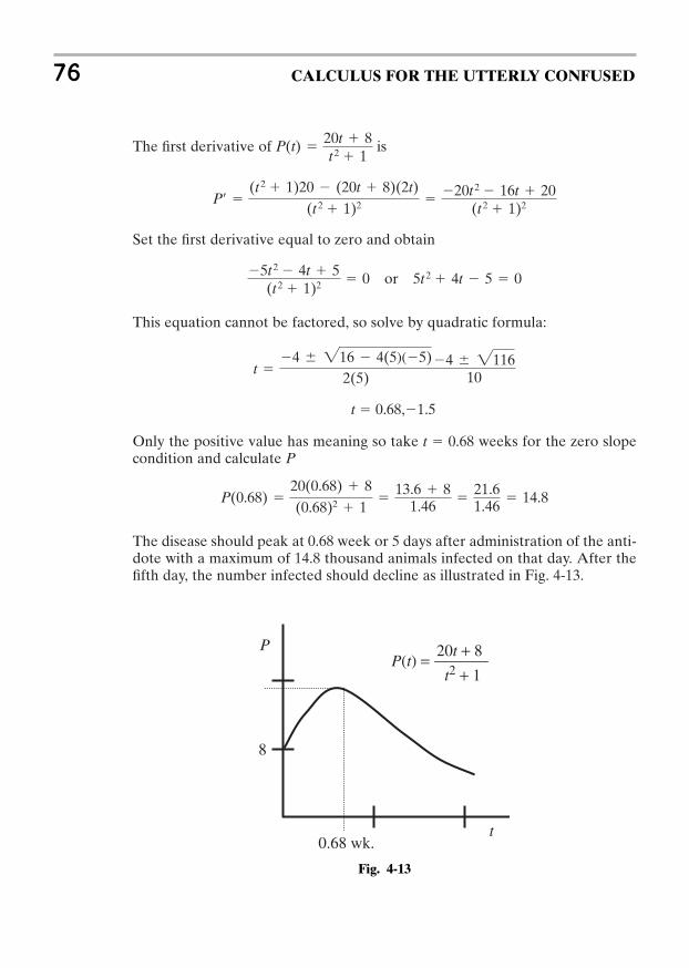
The first derivative of is
Set the first derivative equal to zero and obtain
This equation cannot be factored, so solve by quadratic formula:
t 0.68,1.5
Only the positive value has meaning so take t 0.68 weeks for the zero slopecondition and calculate P
The disease should peak at 0.68 week or 5 days after administration of the anti-dote with a maximum of 14.8 thousand animals infected on that day. After thefifth day, the number infected should decline as illustrated in Fig. 4-13.
P(0.68) 20(0.68) 8(0.68)2 1
13.6 8
1.46
21.61.46
14.8
t 4 216 4(5)(5)
2(5)4 2116
10
5t 2 4t 5(t 2 1)2 0 or 5t 2 4t 5 0
Pr (t 2 1)20 (20t 8)(2t)
(t 2 1)2 20t 2 16t 20
(t 2 1)2
P(t) 20t 8t 2 1
76 CALCULUS FOR THE UTTERLY CONFUSED
Fig. 4-13
8
0.68 wk.t
P 20t + 8t2 + 1
P(t) =
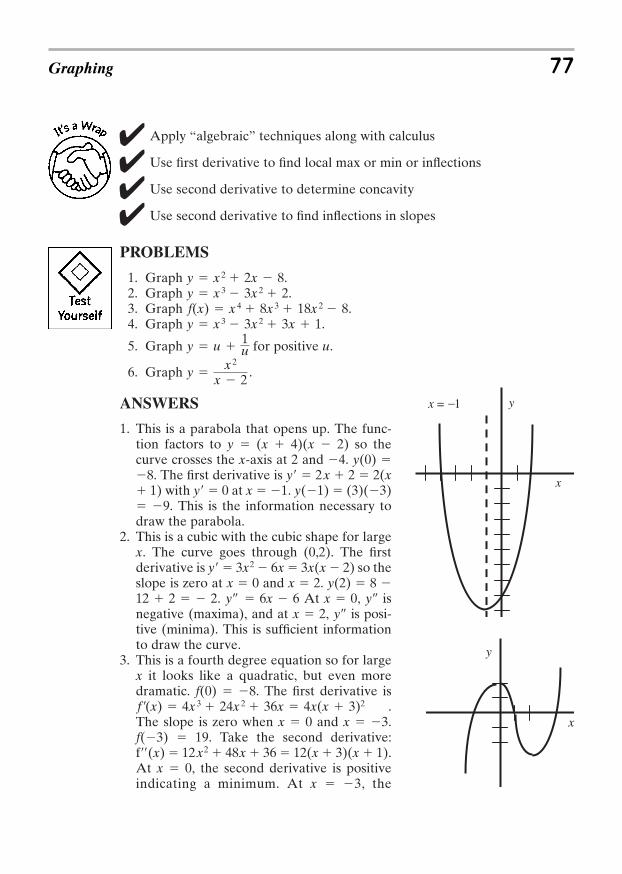
Apply “algebraic” techniques along with calculus
Use first derivative to find local max or min or inflections
Use second derivative to determine concavity
Use second derivative to find inflections in slopes
PROBLEMS
1. Graph .2. Graph .3. Graph .4. Graph .
5. Graph for positive u.
6. Graph .
ANSWERS
1. This is a parabola that opens up. The func-tion factors to y (x 4)(x 2) so thecurve crosses the x-axis at 2 and 4. y(0) 8. The first derivative is y 2x 2 2(x 1) with y 0 at x 1. y(1) (3)(3) 9. This is the information necessary todraw the parabola.
2. This is a cubic with the cubic shape for largex. The curve goes through (0,2). The firstderivative is y 3x2 6x 3x(x 2) so theslope is zero at x 0 and x 2. y(2) 8 12 2 2. At x 0, isnegative (maxima), and at x 2, is posi-tive (minima). This is sufficient informationto draw the curve.
3. This is a fourth degree equation so for largex it looks like a quadratic, but even moredramatic. f(0) 8. The first derivative is
.The slope is zero when x 0 and x 3.f(3) 19. Take the second derivative:f(x) 12x2 48x 36 12(x 3)(x 1).At x 0, the second derivative is positiveindicating a minimum. At x 3, the
f r(x) 4x 3 24x 2 36x 4x(x 3)2
yrryrryrr 6x 6
y x 2
x 2
y u 1u
y x 3 3x 2 3x 1f(x) x 4 8x 3 18x 2 8y x 3 3x 2 2y x 2 2x 8
Graphing 77
x
yx = 1−
x
y
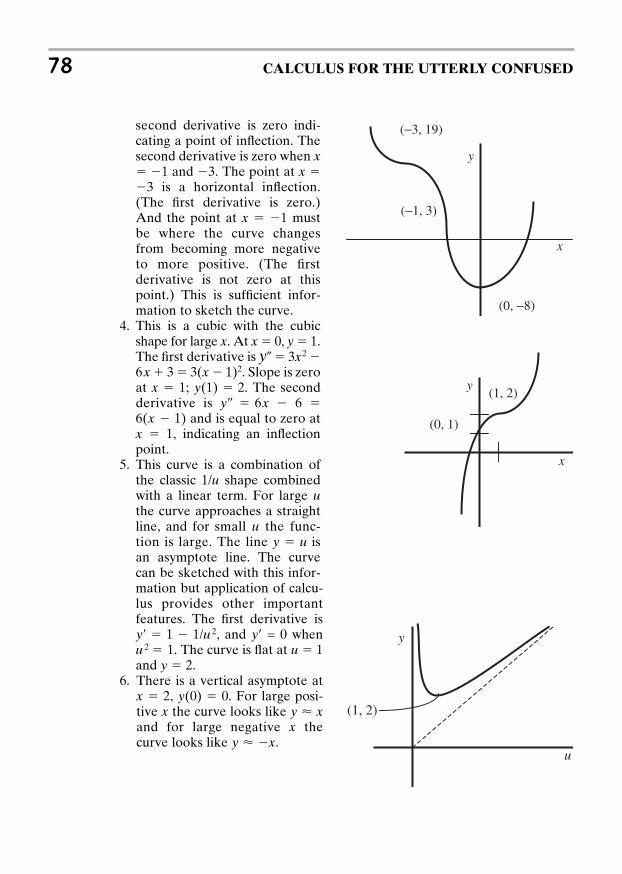
78 CALCULUS FOR THE UTTERLY CONFUSED
second derivative is zero indi-cating a point of inflection. Thesecond derivative is zero when x 1 and 3. The point at x 3 is a horizontal inflection.(The first derivative is zero.)And the point at x 1 mustbe where the curve changesfrom becoming more negativeto more positive. (The firstderivative is not zero at thispoint.) This is sufficient infor-mation to sketch the curve.
4. This is a cubic with the cubicshape for large x. At x 0, y 1.The first derivative is y 3x2 6x 3 3(x 1)2. Slope is zeroat x 1; . The secondderivative is 6x 6 6(x 1) and is equal to zero atx 1, indicating an inflectionpoint.
5. This curve is a combination ofthe classic 1/u shape combinedwith a linear term. For large uthe curve approaches a straightline, and for small u the func-tion is large. The line y u isan asymptote line. The curvecan be sketched with this infor-mation but application of calcu-lus provides other importantfeatures. The first derivative is
, and = 0 when. The curve is flat at u 1
and y 2.6. There is a vertical asymptote at
x 2, . For large posi-tive x the curve looks like and for large negative x thecurve looks like . y < x
y < xy(0) 0
u 2 1yryr 1 1/u 2
yrr y(1) 2
x
y
(0, −8)
(−1, 3)
(−3, 19)
x
y
(0, 1)
(1, 2)
u
y
(1, 2)
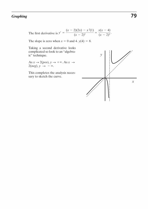
The first derivative is .
The slope is zero when x 0 and 4. .
Taking a second derivative lookscomplicated so look to an “algebra-ic” technique.
As . As x2(neg), y .
This completes the analysis neces-sary to sketch the curve.
SSx S 2(pos), y S `
y(4) 8
yr (x 2)(2x) x 2(1)
(x 2)2 x(x 4)(x 2)2
Graphing 79
x
y

This page intentionally left blank

CHAPTER 5
MAX-MIN PROBLEMS
You should read this chapter if you need to review or you need to learn about
Designing containers for minimum volume
Finding maximum areas for given constraints
Designing beams for maximum strength
Maximum production for agricultural crops
Minimizing production costs
Maximizing profit by price selection
81
Copyright © 2007 by The McGraw-Hill Companies, Inc. Click here for terms of use.
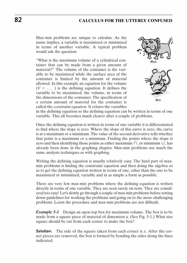
Max-min problems are unique to calculus. As thename implies, a variable is maximized or minimizedin terms of another variable. A typical problemwould ask the question:
“What is the maximum volume of a cylindrical con-tainer that can be made from a given amount ofmaterial?” The volume of the container is the vari-able to be maximized while the surface area of thecontainer is limited by the amount of materialallowed. In this example an equation for the volume( ) is the defining equation. It defines thevariable to be maximized, the volume, in terms ofthe dimensions of the container. The specification ofa certain amount of material for the container iscalled the constraint equation. It relates the variablesin the defining equation so the defining equation can be written in terms of onevariable. This all becomes much clearer after a couple of problems.
Once the defining equation is written in terms of one variable it is differentiatedto find where the slope is zero. Where the slope of this curve is zero, the curveis at a maximum or a minimum. The value of the second derivative tells whetherthat point is a maximum or a minimum. Finding the points where the slope iszero and then identifying those points as either maximum , or minimum , hasalready been done in the graphing chapter. Max-min problems use much thesame analysis techniques as with graphing.
Writing the defining equation is usually relatively easy. The hard part of max-min problems is finding the constraint equation and then doing the algebra soas to get the defining equation written in terms of one, other than the one to bemaximized or minimized, variable and in as simple a form as possible.
There are very few max-min problems where the defining equation is writtendirectly in terms of one variable. They are seen rarely on tests. They are consid-ered too easy! Let’s slowly go through a couple of max-min problems before settingdown guidelines for working the problems and going on to the more challengingproblems. Learn the procedure and max-min problems are not difficult.
Example 5-1 Design an open-top box for maximum volume. The box is to bemade from a square piece of material of dimension a. (See Fig. 5-1.) What sizesquare should be cut from each corner to make the box?
Solution: The side of the square taken from each corner is x. After the cor-ner pieces are removed, the box is formed by bending the sides along the linesindicated.
´¨
V c
82 CALCULUS FOR THE UTTERLY CONFUSED
Max
Min
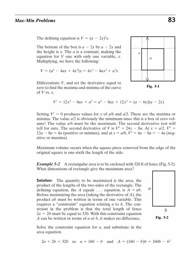
The defining equation is .
The bottom of the box is by andthe height is x. The a is a constant, making theequation for V one with only one variable, x.Multiplying, we have the following:
Differentiate V, and set the derivative equal tozero to find the maxima and minima of the curveof V vs. x.
Setting produces values for x of a/6 and a/2. These are the maxima orminima. The value a/2 is obviously the minimum since this is a box of zero vol-ume! The value a/6 must be the maximum. The second derivative test willtell for sure. The second derivative of V is V 24x 8a. At x a/2, V 12a 8a 4a (positive or minima), and at x a/6, V 4a 8a 4a (neg-ative or maxima).
Maximum volume occurs when the square piece removed from the edge of theoriginal square is one-sixth the length of the side.
Example 5-2 A rectangular area is to be enclosed with 320 ft of fence (Fig. 5-2).What dimensions of rectangle give the maximum area?
Solution: The quantity to be maximized is the area, theproduct of the lengths of the two sides of the rectangle. Thedefining equation, the A equals . . . equation, is .Before maximizing the area (taking the derivative of A), theproduct ab must be written in terms of one variable. Thisrequires a “constraint” equation relating a to b. The con-straint in the problem is that the total length of fence
must be equal to 320. With this constraint equationA can be written in terms of a or b, it makes no difference.
Solve the constraint equation for a, and substitute in thearea equation.
so and A (160 b)b 160b b2a 160 b2a 2b 320
2a 2b
A ab
Vr 0
Vr 12x2 8ax a2 a2 8ax 12x2 (a 6x)(a 2x)
V (a2 4ax 4x2)x 4x3 4ax2 a 2x
a 2xa 2x
V (a 2x)2x
Max-Min Problems 83
Fig. 5-1
Fig. 5-2
ax
a
b
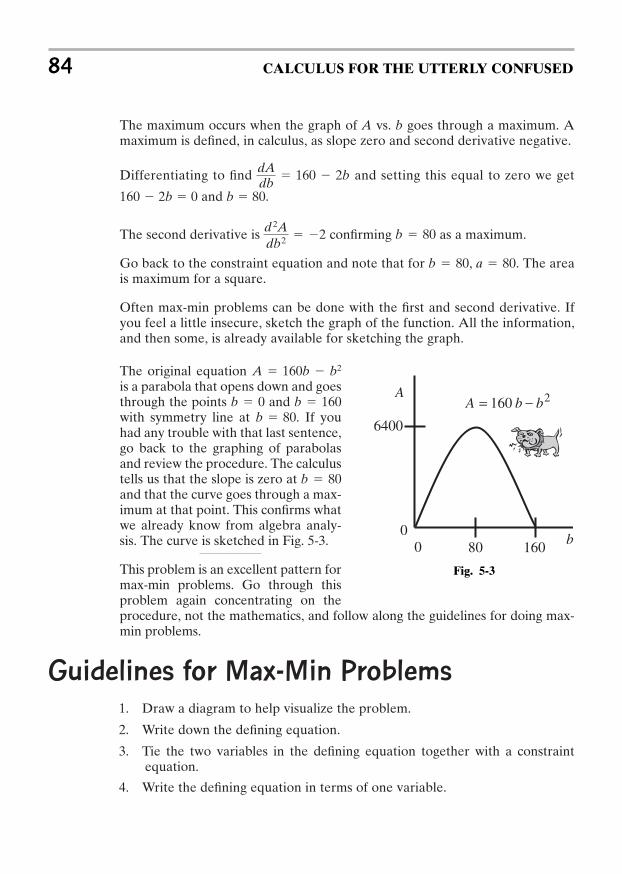
The maximum occurs when the graph of A vs. b goes through a maximum. Amaximum is defined, in calculus, as slope zero and second derivative negative.
Differentiating to find and setting this equal to zero we get
160 2b 0 and b 80.
The second derivative is confirming as a maximum.
Go back to the constraint equation and note that for , . The areais maximum for a square.
Often max-min problems can be done with the first and second derivative. Ifyou feel a little insecure, sketch the graph of the function. All the information,and then some, is already available for sketching the graph.
The original equation is a parabola that opens down and goesthrough the points and with symmetry line at . If youhad any trouble with that last sentence,go back to the graphing of parabolasand review the procedure. The calculustells us that the slope is zero at and that the curve goes through a max-imum at that point. This confirms whatwe already know from algebra analy-sis. The curve is sketched in Fig. 5-3.
This problem is an excellent pattern formax-min problems. Go through thisproblem again concentrating on theprocedure, not the mathematics, and follow along the guidelines for doing max-min problems.
Guidelines for Max-Min Problems
1. Draw a diagram to help visualize the problem.
2. Write down the defining equation.
3. Tie the two variables in the defining equation together with a constraintequation.
4. Write the defining equation in terms of one variable.
b 80
b 80b 160b 0
A 160b b2
a 80b 80
b 80d 2Adb2 2
dAdb
160 2b
84 CALCULUS FOR THE UTTERLY CONFUSED
Fig. 5-3
6400
16080b
A
00
2160 bbA _=
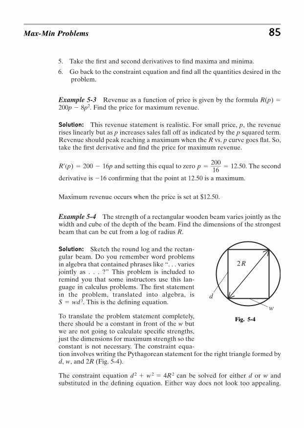
5. Take the first and second derivatives to find maxima and minima.
6. Go back to the constraint equation and find all the quantities desired in theproblem.
Example 5-3 Revenue as a function of price is given by the formula R(p) 200p 8p2. Find the price for maximum revenue.
Solution: This revenue statement is realistic. For small price, p, the revenuerises linearly but as p increases sales fall off as indicated by the p squared term.Revenue should peak reaching a maximum when the R vs. p curve goes flat. So,take the first derivative and find the price for maximum revenue.
and setting this equal to zero . The second
derivative is 16 confirming that the point at 12.50 is a maximum.
Maximum revenue occurs when the price is set at $12.50.
Example 5-4 The strength of a rectangular wooden beam varies jointly as thewidth and cube of the depth of the beam. Find the dimensions of the strongestbeam that can be cut from a log of radius R.
Solution: Sketch the round log and the rectan-gular beam. Do you remember word problemsin algebra that contained phrases like “. . . variesjointly as . . . ?” This problem is included toremind you that some instructors use this lan-guage in calculus problems. The first statementin the problem, translated into algebra, is
. This is the defining equation.
To translate the problem statement completely,there should be a constant in front of the w butwe are not going to calculate specific strengths,just the dimensions for maximum strength so theconstant is not necessary. The constraint equa-tion involves writing the Pythagorean statement for the right triangle formed byd, w, and 2R (Fig. 5-4).
The constraint equation can be solved for either d or w andsubstituted in the defining equation. Either way does not look too appealing.
d 2 w 2 4R 2
S wd 3
p 20016
12.50Rr(p) 200 16p
Max-Min Problems 85
Fig. 5-4
w
d
R2
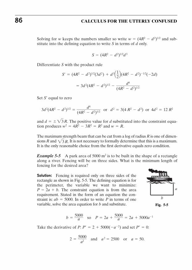
Solving for w keeps the numbers smaller so write and sub-stitute into the defining equation to write S in terms of d only.
Differentiate S with the product rule
Set equal to zero
and . The positive value for d substituted into the constraint equa-tion produces and .
The maximum strength beam that can be cut from a log of radius R is one of dimen-sions R and It is not necessary to formally determine that this is a maximum.It is the only reasonable choice from the first derivative equals zero condition.
Example 5-5 A park area of 5000 m2 is to be built in the shape of a rectanglealong a river. Fencing will be on three sides. What is the minimum length offencing for the desired area?
Solution: Fencing is required only on three sides of therectangle as shown in Fig. 5-5. The defining equation is forthe perimeter, the variable we want to minimize:
. The constraint equation is from the arearequirement. Stated in the form of an equation the con-straint is: . In order to write P in terms of onevariable, solve the area equation for b and substitute.
so
Take the derivative of P: and set :
and or .a 50a 2 25002 5000
a2
Pr 0Pr 2 5000(a2)
P 2a 5000
a 2a 5000a1b 5000
a
ab 5000
P 2a b
23 R.
w Rw2 4R2 3R2 R2d 23 R
3d 2(4R2 d 2)1/2 d4
(4R2 d 2)1/2 or d 2 3(4 R2 d 2) or 4d 2 12 R2
Sr
3d 2(4R2 d 2)1/2 d4
(4R2 d 2)1/2
Sr (4R2 d 2)1/2(3d 2) d 3Q12R(4R2 d 2)1/2(2d)
S (4R2 d 2)1/2d 3
w (4R2 d 2)1/2
86 CALCULUS FOR THE UTTERLY CONFUSED
Fig. 5-5
a
b
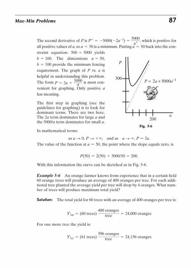
The second derivative of P is , which is positive forall positive values of a, so is a minimum. Putting back into the con-straint equation: yields
. The dimensions ,provide the minimum fencing
requirement. The graph of P vs. a ishelpful in understanding this problem.The form is most con-venient for graphing. Only positive a
has meaning.
The first step in graphing (see theguidelines for graphing) is to look fordominant terms. There are two here.The 2a term dominates for large a andthe 5000/a term dominates for small a.
In mathematical terms:
as , ; and as , .The value of the function at , the point where the slope equals zero, is
.
With this information the curve can be sketched as in Fig. 5-6.
Example 5-6 An orange farmer knows from experience that in a certain field60 orange trees will produce an average of 400 oranges per tree. For each addi-tional tree planted the average yield per tree will drop by 4 oranges. What num-ber of trees will produce maximum total yield?
Solution: The total yield for 60 trees with an average of 400 oranges per tree is:
For one more tree the yield is:
Y Z61 (61 trees) 396 oranges
tree 24,156 oranges
Y Z60 (60 trees) 400 oranges
tree 24,000 oranges
P(50) 2(50) 5000/50 200
a 50P < 2aa S `P S `a S 0
P 2a 5000
a
b 100a 50b 100
50b 5000a 50a 50
Prr 5000(2a3) 5000
a 3
Max-Min Problems 87
Fig. 5-6
300 15000a2 += aP
a
P
200
_
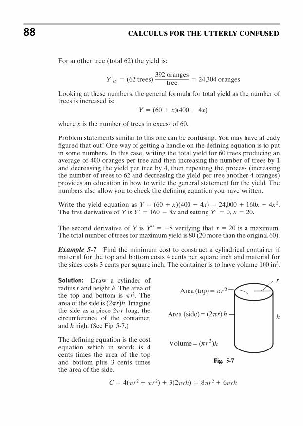
For another tree (total 62) the yield is:
Looking at these numbers, the general formula for total yield as the number oftrees is increased is:
where x is the number of trees in excess of 60.
Problem statements similar to this one can be confusing. You may have alreadyfigured that out! One way of getting a handle on the defining equation is to putin some numbers. In this case, writing the total yield for 60 trees producing anaverage of 400 oranges per tree and then increasing the number of trees by 1and decreasing the yield per tree by 4, then repeating the process (increasingthe number of trees to 62 and decreasing the yield per tree another 4 oranges)provides an education in how to write the general statement for the yield. Thenumbers also allow you to check the defining equation you have written.
Write the yield equation as .The first derivative of Y is and setting , .
The second derivative of Y is verifying that is a maximum.The total number of trees for maximum yield is 80 (20 more than the original 60).
Example 5-7 Find the minimum cost to construct a cylindrical container ifmaterial for the top and bottom costs 4 cents per square inch and material forthe sides costs 3 cents per square inch. The container is to have volume 100 in3.
Solution: Draw a cylinder ofradius r and height h. The area ofthe top and bottom is . Thearea of the side is . Imaginethe side as a piece long, thecircumference of the container,and h high. (See Fig. 5-7.)
The defining equation is the costequation which in words is 4cents times the area of the topand bottom plus 3 cents timesthe area of the side.
C 4(pr 2 pr 2) 3(2prh) 8pr 2 6prh
2pr(2pr)h
pr2
x 20Yrr 8
x 20Yr 0Yr 160 8xY (60 x)(400 4x) 24,000 160x 4x 2
Y (60 x)(400 4x)
Y Z62 (62 trees) 392 oranges
tree 24,304 oranges
88 CALCULUS FOR THE UTTERLY CONFUSED
Fig. 5-7
h(2p r)Area (side) = h
r2(top)Area p r=
p r )h(Volume 2=

The constraint is that the volume must be 100 in3. The volume of a cylindricalcontainer is the area of the bottom, , times the height, h: .
Set , solve for h, and substitute into the defining equation: or and
The first derivative of C is: and setting produces
or and
The second derivative of C is:
is positive for all positive r indicating a minimum for the curve.
Substituting the r for zero slope back into the constraint equation produces
or
Example 5-8 Postal rates increase when the girth (once around) plus thelength of a package exceeds 84 in (Fig. 5-8).What are the dimensions of a “brick-shaped” box with square ends to providemaximum volume?
Solution: The defining equation is thevolume, which in this case is the area of theend, x2, times the length, y: V x2y.
The constraint is that the girth, 4x, plus thelength, y, is limited to 84: 4x y 84.
The simplest way to write the equation in one variable is to solve the con-straint equation for y: and sub-stitute for y in the defining equation.
V x 2(84 4x) 84x2 4x 3
y 84 4x
V c
h 100p ¢16p
600≤ 2/3
< 6.1100 p¢ 60016p
≤ 2/3
h
100 pr 2h
Crr
Crr 16p 1200
r 3
r Å3 600
16p< 2.3r 3
60016p
16pr 600r 2 0
Cr 0Cr 16pr 600r2
C 8pr 2 6pr 100pr 2 8pr 2
600r 8pr 2 600r1
h 100/pr 2100 pr2hV 100
V pr2hpr 2
Max-Min Problems 89
Fig. 5-8
yx
x
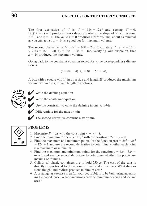
The first derivative of V is and setting ,produces two values of x where the slope of V vs. x is zero:
and . The value produces a zero volume, about as minimalas you can get, so is a good bet for maximum volume.
The second derivative of V is . Evaluating at isverifying our suspicion that
produced the maximum volume.
Going back to the constraint equation solved for y, the corresponding y dimen-sion is
.
A box with a square end 14 in on a side and length 28 produces the maximumvolume within the girth and length restrictions.
Write the defining equation
Write the constraint equation
Use the constraint to write the defining in one variable
Differentiate for the max or min
The second derivative confirms max or min
PROBLEMS
1. Maximize with the constraint .2. Find the minimum for with the constraint .3. Find the maximum and minimum points for the function f(x) 2x 3 3x 2
12x 1 and use the second derivative to determine whether each pointis a maximum or minimum.
4. Find the maximum and minimum points for the function y 4x3 + 3x2 6x + 1 and use the second derivative to determine whether the points aremaxima or minima.
5. Cylindrical plastic containers are to hold 750 cc. The cost of the cans isdirectly proportional to the amount of material in the cans. What dimen-sions (height and radius) produce minimum cost?
6. A rectangular exercise area for your pet rabbit is to be built using an exist-ing L-shaped fence. What dimensions provide minimum fencing and 250 m2
area?
2x y 8G x 2 y 2x y 8P xy
y 84 4(14) 84 56 28
x 14Vrr(14) 168 24(14) 168 336 168
x 14VrrVrr 168 24x
x 14x 0x 14x 0
12x(14 x) 0Vr 0Vr 168x 12x 2
90 CALCULUS FOR THE UTTERLY CONFUSED
7. In a certain manufacturing operation there are at present 40 workers, eachworker capable of producing 50 items per day. For each two additionalworkers production per worker drops by 1 item per day. What is the num-ber of workers for maximum production?
8. Marketing experience indicates that the revenue from the release of aDVD follows where p is the price of the DVD.What is the price for maximum revenue?
9. A clothing manufacturer makes sweat shirts. The cost of making x shirts
(valid on production runs up to 500) follows: .
The average cost per shirt is this function divided by the number of shirts
produced. . Find the production run
that has the lowest cost per shirt.
10. You need to make open top boxes from an 8 18 in rectangle of materialby cutting squares out of the corners and folding up the sides. Design thelargest volume box that can be made this way.
ANSWERS
1. Substitute for x in the defining equation: and takethe derivative. . Set this derivative to zero and find y 4. Thesecond derivative is negative everywhere so this is a maximum. Values of
and produce maximum P.2. Substitute for y. . The first deriva-
tive is . This gives x 3.2 as the minimum. The secondderivative is always positive so this is a minimum.
3. The first derivative is which is zero for x 1 and x 2.
The second derivative is is positive for x 1, indicating a
minimum for x 1, and negative for x 2, indicating a maximum, for
x 2.4. The first derivative is . The curve has extrema at 1/2
and 1. The second derivative is , which is positive at 1/2indicating a minimum at this point, and negative at x (1 indicating a max-imum at this point.
5. We need to minimize the area. (Area is directly related to cost.) The areaof the ends is each and the area of the cylinder walls is the circumfer-ence of the end caps times the height of the cylinder: . The volume isthe constraint and the volume is the area of the end caps times the height
. The constraint equation is , and the defining equation is750 pr 2hpr 2h
2prhpr 2
yrr 24x 6yr 12x2 6x 6
d 2f
dx 2 12x 6
dfdx
6x2 6x 12
Gr 10x 32G x 2 (8 2x)2 5x 2 32x 64
y 4x 4
Pr 8 2yP (8 y)y 8y y 2
C(x) C(x)
x 2000x1 10 0.2x
C(x) 2000 10x 0.2x 2
R 20,000p 1000p 2
Max-Min Problems 91
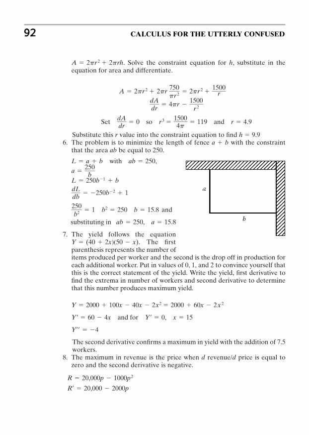
. Solve the constraint equation for h, substitute in theequation for area and differentiate.
Set
Substitute this r value into the constraint equation to find h 9.96. The problem is to minimize the length of fence a b with the constraint
that the area ab be equal to 250.
7. The yield follows the equation. The first
parenthesis represents the number ofitems produced per worker and the second is the drop off in production foreach additional worker. Put in values of 0, 1, and 2 to convince yourself thatthis is the correct statement of the yield. Write the yield, first derivative tofind the extrema in number of workers and second derivative to determinethat this number produces maximum yield.
The second derivative confirms a maximum in yield with the addition of 7.5workers.
8. The maximum in revenue is the price when d revenue/d price is equal tozero and the second derivative is negative.
Rr 20,000 2000p
R 20,000p 1000p2
Yrr 4
Y r 60 4x and for Y r 0, x 15
Y 2000 100x 40x 2x2 2000 60x 2x 2
Y (40 2x)(50 x)
substituting in ab 250, a 15.8
250b2 1 b2 250 b 15.8 and
dLdb
250b2 1
L 250b1 b
a 250b
L a b with ab 250,
dAdr
0 so r 3 15004p 119 and r 4.9
dAdr
4pr 1500
r 2
A 2pr 2 2pr 750pr 2 2pr 2
1500r
A 2pr 2 2prh
92 CALCULUS FOR THE UTTERLY CONFUSED
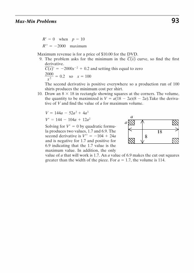
Maximum revenue is for a price of $10.00 for the DVD.9. The problem asks for the minimum in the curve, so find the first
derivative.and setting this equal to zero
so x 100
The second derivative is positive everywhere so a production run of 100shirts produces the minimum cost per shirt.
10. Draw an 8 18 in rectangle showing squares at the corners. The volume,the quantity to be maximized is .Take the deriva-tive of V and find the value of a for maximum volume.
Solving for by quadratic formu-la produces two values, 1.7 and 6.9. Thesecond derivative is and is negative for 1.7 and positive for6.9 indicating that the 1.7 value is themaximum value. In addition, the onlyvalue of a that will work is 1.7. An a value of 6.9 makes the cut out squaresgreater than the width of the piece. For a 1.7, the volume is 114.
Vrr 104 24a
Vr 0
Vr 144 104a 12a2
V 144a 52a 2 4a3
V a(18 2a)(8 2a)
2000x 2 0.2
C(x)r 2000x2 0.2
C(x)
Rrr 2000 maximum
Rr 0 when p 10
Max-Min Problems 93

This page intentionally left blank
CHAPTER 6
RELATED RATEPROBLEMS
You should read this chapter if you need to review or you need to learn about
Find related rates through implicit differentiation
Solve distance-related rates
Related rates for moving bodies
Geometric-related rates
Area-related rates
Volume-related rates
95
Copyright © 2007 by The McGraw-Hill Companies, Inc. Click here for terms of use.
Related rate problems relate one rate, written as a derivative, to another rate writ-ten as a derivative. An excellent example of a related rate problem, and one that isin nearly every calculus book including this one, is a ladder sliding down a wall. (SeeFig. 6-1.) The top of the ladder is moving down the wall while the bottom of the lad-der is moving away from the wall. The rate (speed) the top is moving down the wallcan be related to the rate (speed) the bottom is moving away from the wall. Thisproblem illustrates well the name of these problems; related rate problems.
A little review is in order. Related rate problems are similar to problems involvingimplicit differentiation. Equations in the form such as are differentiated term by term according to the rules for differentiating polyno-mials, products, quotients, or whatever. Equations where the x’s and y’s are mixedtogether so the equation cannot be written as or (an x alone ora y alone on one side of the equation) are differentiated implicitly.
For example, the equation must be differentiated implicitly as
with formed by grouping and rearranging.
If x and y could both change over time then a related rate associated differen-tiation of this equation would be
In this statement, is directly related to
or
This is an example of a related rate differentiation. Now take a look at perhapsnot the simplest related rate problem, but possibly the simplest to visualize.Notice how this problem is written. The general situation is described, then arate is specified and the related rate is requested for a certain condition.
Example 6-1 A 7-m-long ladder is sliding down a wall. The bottom of theladder is pulled from the wall at What is the rate at which the top of theladder is going down when the bottom is from the wall?
Solution: Help to visualize the problem by sketching a ladder leaning against awall with the bottom being pulled out from the wall at (Fig. 6-1).dx/dt 1.5 m/s
3 m1.5 m/s.
dxdt
4xy 3xy2
2y2 y3
dydt
(2y2 y3) dxdt
(4xy 3xy2)dydt
dydt
dxdt
2y2 dxdt
4xydydt
3xy2dydt
y3 dxdt
0
dy/dx
2y2dx 4xydy 3xy2dy y3dx 0
2xy2 xy3 0
x f(y)y f(x)
y x2 2x 3y f(x)
96 CALCULUS FOR THE UTTERLY CONFUSED
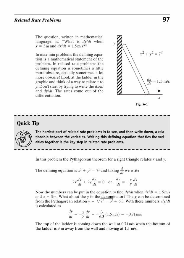
The question, written in mathematicallanguage, is: “What is when
and ?”
In max-min problems the defining equa-tion is a mathematical statement of theproblem. In related rate problems thedefining equation is sometimes a littlemore obscure, actually sometimes a lotmore obscure! Look at the ladder in thegraphic and think of a way to relate x toy. Don’t start by trying to write the and The rates come out of thedifferentiation.
dy/dt.dx/dt
dx/dt 1.5 m/sx 3 mdy/dt
Related Rate Problems 97
Quick Tip
The hardest part of related rate problems is to see, and then write down, a rela-
tionship between the variables. Writing this defining equation that ties the vari-
ables together is the key step in related rate problems.
Fig. 6-1
In this problem the Pythagorean theorem for a right triangle relates x and y.
The defining equation is and taking we write
or
Now the numbers can be put in the equation to find when and . What about the y in the denominator? The y can be determinedfrom the Pythagorean relation . With these numbers, is calculated as
The top of the ladder is coming down the wall at when the bottom ofthe ladder is 3 m away from the wall and moving at .1.5 m/s
0.71 m/s
dydt
xy
dxdt
3
6.3 (1.5 m/s) 0.71 m/s
dy/dty 272 32 < 6.3x 3 m
dx/dt 1.5 m/sdy/dt
dydt
xy
dxdt
2x dxdt
2ydydt
0
ddt
x2 y2 72
m/s5.1=dtdx
y
x
222 7=+ yx
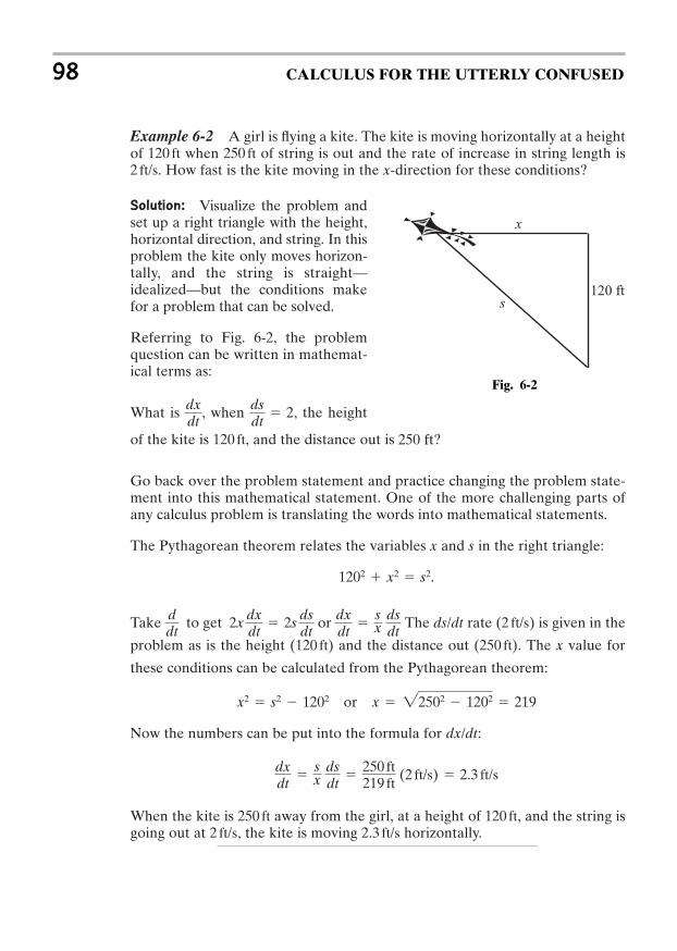
Example 6-2 A girl is flying a kite. The kite is moving horizontally at a heightof when of string is out and the rate of increase in string length is
. How fast is the kite moving in the x-direction for these conditions?
Solution: Visualize the problem andset up a right triangle with the height,horizontal direction, and string. In thisproblem the kite only moves horizon-tally, and the string is straight—idealized—but the conditions makefor a problem that can be solved.
Referring to Fig. 6-2, the problemquestion can be written in mathemat-ical terms as:
What is , when , the height
of the kite is , and the distance out is 250 ft?
Go back over the problem statement and practice changing the problem state-ment into this mathematical statement. One of the more challenging parts ofany calculus problem is translating the words into mathematical statements.
The Pythagorean theorem relates the variables x and s in the right triangle:
.
Take to get or The rate is given in the
problem as is the height and the distance out . The x value for
these conditions can be calculated from the Pythagorean theorem:
or
Now the numbers can be put into the formula for :
When the kite is away from the girl, at a height of , and the string isgoing out at , the kite is moving horizontally.2.3 ft/s2 ft/s
120 ft250 ft
dxdt
sx
dsdt
250 ft219 ft
(2 ft/s) 2.3 ft/s
dx/dt
x 22502 1202 219x2 s2 1202
(250 ft)(120 ft)
(2 ft/s)ds/dtdxdt
sx
dsdt
2x dxdt
2s dsdt
ddt
1202 x2 s2
120 ft
dsdt
2dxdt
2 ft/s250 ft120 ft
98 CALCULUS FOR THE UTTERLY CONFUSED
Fig. 6-2
x
120 fts
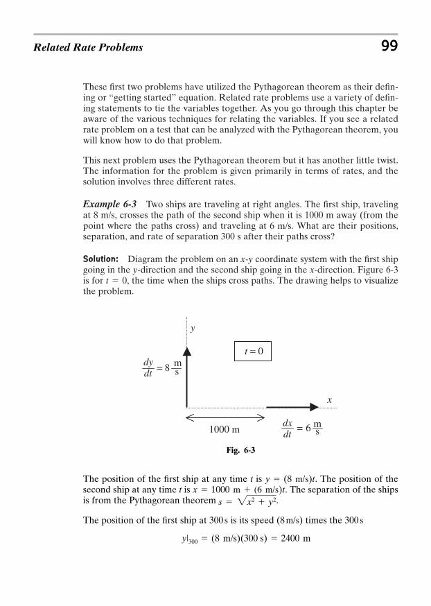
These first two problems have utilized the Pythagorean theorem as their defin-ing or “getting started” equation. Related rate problems use a variety of defin-ing statements to tie the variables together. As you go through this chapter beaware of the various techniques for relating the variables. If you see a relatedrate problem on a test that can be analyzed with the Pythagorean theorem, youwill know how to do that problem.
This next problem uses the Pythagorean theorem but it has another little twist.The information for the problem is given primarily in terms of rates, and thesolution involves three different rates.
Example 6-3 Two ships are traveling at right angles. The first ship, travelingat 8 m/s, crosses the path of the second ship when it is 1000 m away (from thepoint where the paths cross) and traveling at 6 m/s. What are their positions,separation, and rate of separation 300 s after their paths cross?
Solution: Diagram the problem on an x-y coordinate system with the first shipgoing in the y-direction and the second ship going in the x-direction. Figure 6-3is for , the time when the ships cross paths. The drawing helps to visualizethe problem.
t 0
Related Rate Problems 99
Fig. 6-3
sm8=dt
dy
sm6=
dtdx
1000 m
y
x
t = 0
The position of the first ship at any time t is . The position of thesecond ship at any time t is . The separation of the shipsis from the Pythagorean theorem .
The position of the first ship at is its speed times the
y|300 (8 m/s)(300 s) 2400 m
300 s(8 m/s)300 s
s 2x2 y2
x 1000 m (6 m/s)ty (8 m/s)t
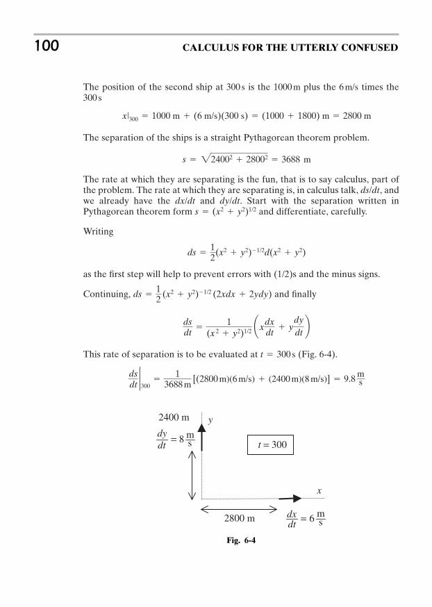
The position of the second ship at is the plus the times the
The separation of the ships is a straight Pythagorean theorem problem.
The rate at which they are separating is the fun, that is to say calculus, part ofthe problem. The rate at which they are separating is, in calculus talk, , andwe already have the and . Start with the separation written inPythagorean theorem form and differentiate, carefully.
Writing
as the first step will help to prevent errors with (1/2)s and the minus signs.
Continuing, and finally
This rate of separation is to be evaluated at (Fig. 6-4).
dsdt2300
1
3688 m[(2800 m)(6 m/s) (2400 m)(8 m/s)] 9.8 m
s
t 300 s
dsdt
1
(x 2 y2)1/2 ¢xdxdt
ydydt≤
ds 12 (x2 y2)1/2 (2xdx 2ydy)
ds 12(x2 y2)1/2d(x2 y2)
s (x2 y2)1/2dy/dtdx/dt
ds/dt
s 224002 28002 3688 m
x|300 1000 m (6 m/s)(300 s) (1000 1800) m 2800 m
300 s6 m/s1000 m300 s
100 CALCULUS FOR THE UTTERLY CONFUSED
Fig. 6-4
2400 m
sm8=
dtdy
sm6=
dtdx2800 m
y
x
t = 300
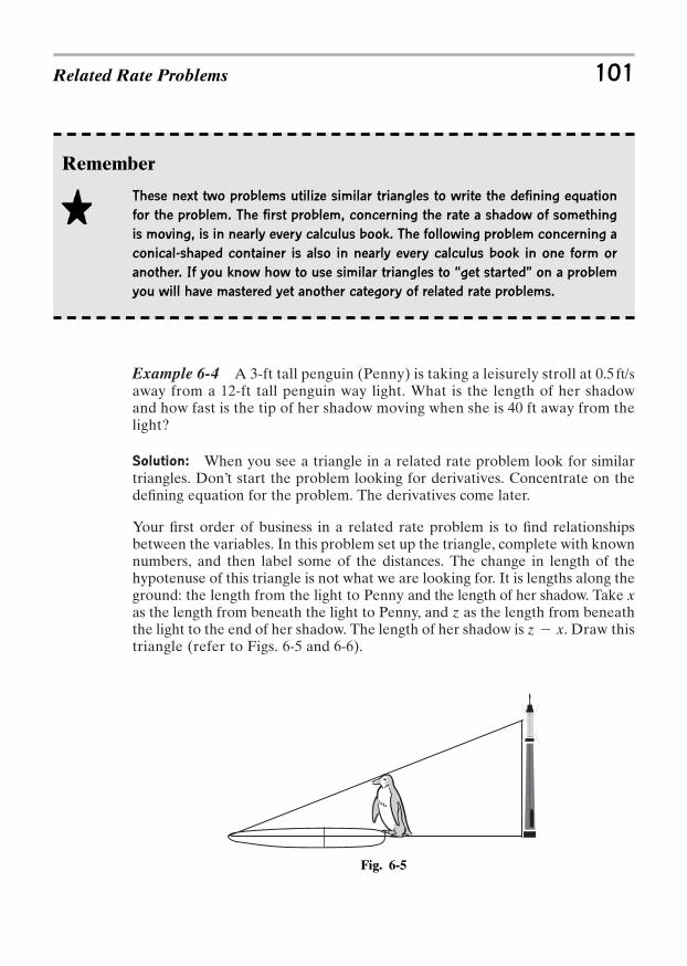
Example 6-4 A 3-ft tall penguin (Penny) is taking a leisurely stroll at away from a 12-ft tall penguin way light. What is the length of her shadowand how fast is the tip of her shadow moving when she is 40 ft away from thelight?
Solution: When you see a triangle in a related rate problem look for similartriangles. Don’t start the problem looking for derivatives. Concentrate on thedefining equation for the problem. The derivatives come later.
Your first order of business in a related rate problem is to find relationshipsbetween the variables. In this problem set up the triangle, complete with knownnumbers, and then label some of the distances. The change in length of thehypotenuse of this triangle is not what we are looking for. It is lengths along theground: the length from the light to Penny and the length of her shadow. Take xas the length from beneath the light to Penny, and z as the length from beneaththe light to the end of her shadow. The length of her shadow is . Draw thistriangle (refer to Figs. 6-5 and 6-6).
z x
0.5 ft/s
Related Rate Problems 101
Fig. 6-5
Remember
These next two problems utilize similar triangles to write the defining equation
for the problem. The first problem, concerning the rate a shadow of something
is moving, is in nearly every calculus book. The following problem concerning a
conical-shaped container is also in nearly every calculus book in one form or
another. If you know how to use similar triangles to “get started” on a problem
you will have mastered yet another category of related rate problems.
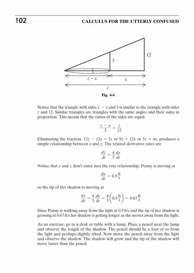
Notice that the triangle with sides and 3 is similar to the triangle with sidesz and 12. Similar triangles are triangles with the same angles and their sides inproportion. This means that the ratios of the sides are equal.
Eliminating the fraction, or or , produces asimple relationship between x and z. The related derivative rates are
Notice that x and z don’t enter into the rate relationship. Penny is moving at
so the tip of her shadow is moving at
Since Penny is walking away from the light at and the tip of her shadow isgrowing at her shadow is getting longer as she moves away from the light.
As an exercise, go to a desk or table with a lamp. Place a pencil near the lampand observe the length of the shadow. The pencil should be a foot or so fromthe light and perhaps slightly tilted. Now move the pencil away from the lightand observe the shadow. The shadow will grow and the tip of the shadow willmove faster than the pencil.
0.67 ft/s0.5 ft/s
dzdt
43
dxdt
43 ¢0.5 ft
s ≤ 0.67 fts
dxdt
0.5 fts
dzdt
43
dxdt
3z 4x9z 12x12z 12x 3z
z x3
z12
z x
102 CALCULUS FOR THE UTTERLY CONFUSED
Fig. 6-6
12
z
z − x x
3
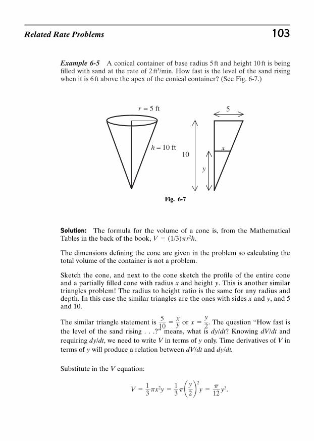
Example 6-5 A conical container of base radius and height is beingfilled with sand at the rate of . How fast is the level of the sand risingwhen it is above the apex of the conical container? (See Fig. 6-7.)6 ft
2 ft3/min10 ft5 ft
Related Rate Problems 103
Fig. 6-7
10 ft=h
5 ft=r 5
10
y
x
Solution: The formula for the volume of a cone is, from the MathematicalTables in the back of the book, .
The dimensions defining the cone are given in the problem so calculating thetotal volume of the container is not a problem.
Sketch the cone, and next to the cone sketch the profile of the entire coneand a partially filled cone with radius x and height y. This is another similartriangles problem! The radius to height ratio is the same for any radius anddepth. In this case the similar triangles are the ones with sides x and y, and 5and 10.
The similar triangle statement is or . The question “How fast isthe level of the sand rising . . .?” means, what is dy/dt? Knowing dV/dt andrequiring dy/dt, we need to write V in terms of y only. Time derivatives of V interms of y will produce a relation between dV/dt and dy/dt.
Substitute in the V equation:
.V 13px2y
13p¢
y2 ≤
2
y p
12y3
x y2
510
xy
V (1/3)pr2h
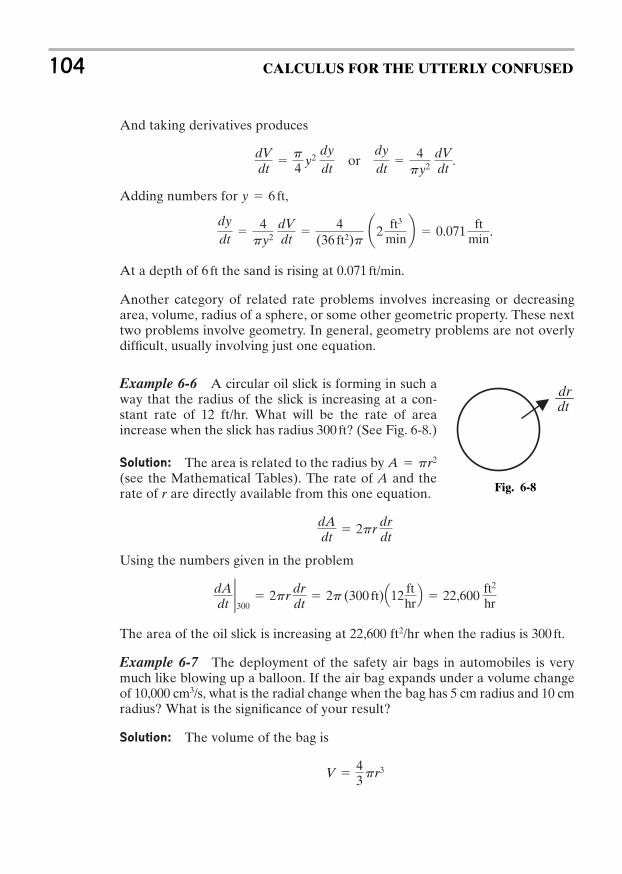
And taking derivatives produces
or .
Adding numbers for ,
.
At a depth of the sand is rising at .
Another category of related rate problems involves increasing or decreasingarea, volume, radius of a sphere, or some other geometric property. These nexttwo problems involve geometry. In general, geometry problems are not overlydifficult, usually involving just one equation.
Example 6-6 A circular oil slick is forming in such away that the radius of the slick is increasing at a con-stant rate of 12 ft/hr. What will be the rate of areaincrease when the slick has radius ? (See Fig. 6-8.)
Solution: The area is related to the radius by (see the Mathematical Tables). The rate of A and therate of r are directly available from this one equation.
Using the numbers given in the problem
The area of the oil slick is increasing at 22,600 ft2/hr when the radius is .
Example 6-7 The deployment of the safety air bags in automobiles is verymuch like blowing up a balloon. If the air bag expands under a volume changeof 10,000 cm3/s, what is the radial change when the bag has 5 cm radius and 10 cmradius? What is the significance of your result?
Solution: The volume of the bag is
V 43pr3
300 ft
dAdt2300
2pr drdt
2p (300 ft)Q12 fthrR 22,600 ft2
hr
dAdt
2pr drdt
A pr2
300 ft
0.071 ft/min6 ft
dydt
4py2
dVdt
4
(36 ft2)p¢2 ft3
min≤ 0.071 ft
min
y 6 ft
dydt
4py2
dVdt
dVdt
p4 y2
dydt
104 CALCULUS FOR THE UTTERLY CONFUSED
Fig. 6-8
dtdr
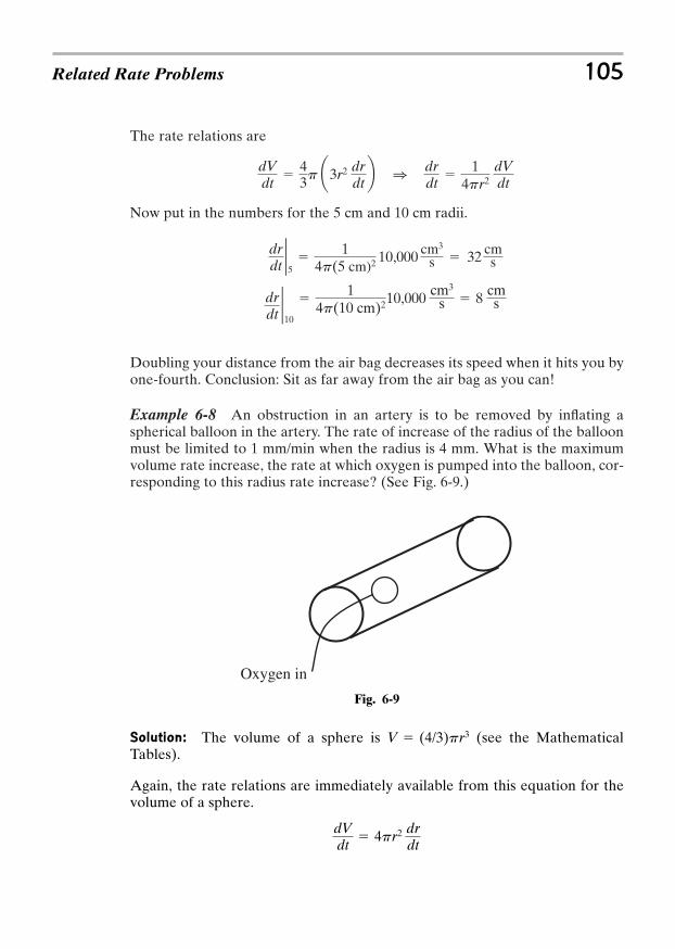
The rate relations are
Now put in the numbers for the 5 cm and 10 cm radii.
Doubling your distance from the air bag decreases its speed when it hits you byone-fourth. Conclusion: Sit as far away from the air bag as you can!
Example 6-8 An obstruction in an artery is to be removed by inflating aspherical balloon in the artery. The rate of increase of the radius of the balloonmust be limited to 1 mm/min when the radius is 4 mm. What is the maximumvolume rate increase, the rate at which oxygen is pumped into the balloon, cor-responding to this radius rate increase? (See Fig. 6-9.)
drdt210
1
4p(10 cm)210,000 cm3
s 8 cms
drdt25
1
4p(5 cm)2 10,000 cm3
s 32 cms
dVdt
43p ¢3r2 dr
dt≤ 1 dr
dt
14pr2
dVdt
Related Rate Problems 105
Fig. 6-9
Oxygen in
Solution: The volume of a sphere is (see the MathematicalTables).
Again, the rate relations are immediately available from this equation for thevolume of a sphere.
dVdt
4pr2 drdt
V (4/3)pr3
Evaluating at and
The maximum rate that the balloon can be filled at the 4 mm radius is.
These last two problems are illustrative of problems where the formulas aregiven to you. In most of these types of problems, differentiating the formula isthe challenge.
Example 6-9 When the price of a certain product is p dollars per unit, cus-tomer demand is x hundreds of units (per month). The relation between p andx is . When the price is $4.00 and dropping at the rate of$0.25 per month, what is the rate of increase in demand?
Solution: This equation requires an implicit type of differentiation to find, the rate of price change, and , the rate of demand change.
or
or
The rate of price change, , is given in the problem as is p, the price.The demand rate, x, is not given and must be computed from the originalequation. Substituting for in yields
or . The quadratic formula produces twoanswers. The positive 5.4 is the realistic one.
With all the needed values, can be evaluated. Watch the signs closely.
dxdt24
2(5.4) 42(5.4) 8
(0.25) 14.818.8
(0.25) 0.20
dx/dt
x 8 264 4(1)(72)
2(1)
8 18.82 5.4,14.4
x2 8x 72 0x2 8x 8 80x2 2px 0.5p2 80(p $4.00)p 4
dp/dt
dxdt
2x p2x 2p
dpdt
(2x 2p) dxdt
(2x p)dpdt
02xdxdt
2p dxdt
2xdpdt
pdpdt
0
dx/dtdp/dt
x2 2px 0.5p2 80
201 mm3/min
dVdt24
4p(4 mm)2 ¢1mmmin
≤ 201 mm3
min
drdt
1 mmmin
r 4 mm
106 CALCULUS FOR THE UTTERLY CONFUSED
The demand rate is increasing by 0.20 hundreds of units per month when the priceis $4.00 and dropping at the rate of $0.25 per month. Carrying the units throughthis problem is difficult because the constants in the original equation must havethe appropriate units to make each term in the equation have the same units.
Example 6-10 The amount of trash, measured in thousands of pounds, accu-mulating in a city dump follows the formula , where p isthe population in hundreds of thousands. What is the rate of trash increase whenthe population is 200 thousand and increasing by 0.2 thousand (0.1%) per month?
Solution: Relating the rate of trash increase, , to the population increase,, comes directly from implicit type differentiation of the expression for the
amount of trash.
The population and the rate of increase in population are given in the problemso we have
[0.2 thousand per month]
84 thousand of pounds per month.
This is also an interesting max-min problem. Take and set
equal to zero to find . The second derivative so the point
is a minimum.
The minimum in trash accumulation rate is at 38 thousand people, but at 200thousand the curve becomes progressively more positive and the trash problemprogressively worse.
Example 6-11 The number of CD players that can be manufactured by a cer-tain company follows a Cobb-Douglas type of production model, where q, theproduction output, depends on the number of workers, n, and the number ofautomatic assembly machines, r, according to . With 20 workersthe company is producing 300 CDs per day and has sufficient revenue to pur-chase one automatic assembly machine per month. How many workers permonth should be laid off to maintain constant production?
q 20 n0.6r0.4
p 38
d 2Tdp 2 2.6p 38
dTdp
(2.6p 100)
dTdt2200
[(2.6)(200) 100]
dTdt
2.6pdpdt
100dpdt
(2.6p 100)dpdt
dp/dtdT/dt
T 1.3p2 100p 30
Related Rate Problems 107
Solution: The first step in the problem is to perform an implicit differentiationremembering that q has to remain constant.
Now write the rate relationship. This could have been written directly.
It takes 20 workers to produce 300 CDs so the number of automatic assemblymachines can be calculated from the original equation.
Now calculate the related rate.
Adding one automatic assembly machine and releasing 1.4 workers per monthwill maintain production.
Relate the variables in the problem
Use a diagram if that will help
Use a variation of implicit differentiation to write the rates
Calculate specific variable values from the defining equation
PROBLEMS
1. For the equation find dy/dt when x 4 and dx/dt 6.2. For find dx/dt when y 2 and dy/dt 3.x2 2xy y2 0
x2 y2 20
dndt
23 ¢ 20
9.7 ≤(1) 1.4
[r 0.4]2.5 r S15
(20)0.6 T2.5
(15)2.5
(20)1.5 9.7
r 0.4 300
(20)(20)0.6 15
200.6
q 20n0.6 r 0.4 1 300 (20)(20)0.6 r 0.4
dndt
23 ¢n
r ≤drdt
0.4 ¢nr ≤ 0.6 dr
dt 0.6¢ r
n ≤ 0.4 dndt
0 20[n0.6(0.4)r0.6dr r0.4(0.6)n0.4dn]
108 CALCULUS FOR THE UTTERLY CONFUSED
3. A rocket launched vertically is tracked by a camera 200 m horizontally awayfrom the launch point. What is the vertical speed of the rocket when it is 600m from the camera with this distance (from the camera) increasing at 80 m/s?
4. The cost in dollars per day to produce thumb drives followswhere x is the number of thumb drives pro-
duced each day. The present production level is 200 thumb drives per dayand this rate is increasing at 2 per day. How fast is the average cost chang-ing? Remember that average cost is C(x) over x.
5. At a price, p, a manufacturer is willing to supply x number of productsaccording to the equation x2 xp p2 30. What is the rate of supply ofx when p is $9.00 and increasing at $0.20 per week?
6. The mass of a raindrop is where is the density of water, 1 g/cm3,and r is the radius of the drop. At what rate is the radius of a raindrop chang-ing when it has a radius of 10 mm and is gaining water at the rate of 0.01 g/min?
7. An observer with a telescope is observing the approach of an airplane trav-eling 700 km/hr towards a point directly over the telescope. The airplaneremains at a constant height of 9.0 km. What is the angular rate of change(in rad/sec) for the telescope when the airplane is 24 km horizontally fromthe telescope?
8. An adiabatic process follows the pressure-volume formula PV1.4 C, aconstant. For P 2 N/m2, V 0.8 m3 and V is increasing at 0.6 m3/s, whatis happening to P.
9. The period, the time for one back-and-forth excursion, of a pendulum is
, where L is the length of the pendulum and g is the acceleration due to gravity equal to 9.8 m/s2. If the length of the pendulum stretchesby 0.01% over 1 year, what is the change in the period?
10. The Poiseuille’s law for flow through a cylindrical pipe (blood vessel) is:, where v is the velocity, K is a constant equal to 6 1/s, L is
the length of the pipe, R is the radius of the pipe and r is the distance outfrom the center line of the pipe. For a 100-cm pipe of radius 0.2 cm, find therate that the flow velocity is changing half-way between the center line andthe wall when the pipe is contracting at a rate of 0.0004 cm/s?
ANSWERS
1. Start with the implicit derivative and proceed to time
derivatives and to . Now stop and calculate y for
x 4. .dydt
42(6) 1242 y2 20 1 y 2 1
dydt
xy
dxdt
ydydt
xdxdt
2xdx 2ydy 0
v KL(R2 r2)
T 2pÅ
Lg
M r43pr3
C(x) 4000 12x x2
200
Related Rate Problems 109
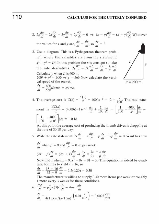
2. Whatever
the values for x and y are, , so .
3. Use a diagram. This is a Pythagorean theorem prob-
lem where the variables are from the statement:
x2 + y2 L2. In this problem the x is constant so take
the rate derivatives.
Calculate y when L is 600 m.Now calculate the verti-
cal speed of the rocket.
4. The average cost is . The rate state-
ment is =
At this point the average cost of producing the thumb drives is dropping atthe rate of $0.18 per day.
5. Write the rate statement: . Want to know
when p 9 and per week.
Now find x when p = 9. x2 9x 81 30 This equation is solved by quad-ratic formula to yield x = 16, so
The manufacturer is willing to supply 0.30 more items per week or roughly1 more every 3 weeks for these conditions.
6.
drdt
1
4(1 g/cm3)p(1 cm)2 ¢0.01g
min≤ 0.0025 cm
min
dMdt
r43p (3)r2dr
dt 4rp r2dr
dt
dxdt
18 1632 9
dpdt
1.5(0.20) 0.30
(2x p)dxdt
(2p x)dpdt1 dx
dt
2p x2x p
dpdt
dpdt
0.20dxdt
2x dxdt
xdpdt
p dxdt
2pdpdt
0
B 1100
40002002 R(2) 0.18
B 1100
4000
x2 Rdxdt
dxdt
1
100dxdt
dC(x)dt
(4000)(1)x2
C(x) C(x)
x 4000x1 12 x
100
dydt
600566
80 m/s 85 m/s
2002 y2 6002 1 y 566
2ydydt
2LdLdt1
dydt
Ly
dLdt
dxdt
3dxdt
dydt
2xdxdt
2xdydt
2ydxdt
2ydydt
0 1 (x y)dxdt
(x y)dydt
110 CALCULUS FOR THE UTTERLY CONFUSED
L
x = 200 m
y
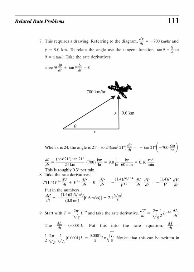
7. This requires a drawing. Referring to the diagram, and
y 9.0 km. To relate the angle use the tangent function, or
. Take the rate derivatives.
x sec 2ududt
tan udxdt
0
9 x tan u
tan u 9x
dxdt
700 km/hr
Related Rate Problems 111
700 km/hr
9.0 km
x
y
q
When x is 24, the angle is 21,
This is roughly 0.3 per min.8. Take the rate derivatives:
Put in the numbers.
9. Start with and take the rate derivative. .
The . Put this into the rate equation.
. Notice that this can be written in12
2p
2g
1
2L(0.0001)L
0.00012 2p
ÅLg
dTdt
dLdt
0.0001 L
dTdt
2p
2g
12 L1/2 dL
dtT
2p
2gL1/2
dPdt
(1.4)(2 N/m2)
(0.8 m3)[0.6 m3/s)] 2.1N/m2
s
P(1.4)V 0.4dVdt
V 1.4 dPdt
0 dPdt
(1.4)PV 0.4
V 1.4dVdt
dPdt
(1.4)P
VdVdt
dudt
(cos221) tan 21
24 km(700) km
hr 9.8 1
hrhr
60 min 0.16
radmin
tan 21¢700 kmhr≤ so 24(sec2 21) du
dt
terms of the original period. . Writing this another way is
instructive. . This states that the fractional change in the
period is 0.00005 per year.
10. Write the general rate statement. Now put in thenumbers.
.dvdt
2 6/s1.0 m
(0.002 m)¢0.0004 cms ≤ 1.0 105 cm
s2
dvdt
KL () 2r dr
dt
dTT 0.00005dt
dTdt
0.00005 T
112 CALCULUS FOR THE UTTERLY CONFUSED

CHAPTER 7
INTEGRATION
You should read this chapter if you need to review or you need to learn about
The antiderivative
Area under the curve
Average value of a function
Area between curves
113
Copyright © 2007 by The McGraw-Hill Companies, Inc. Click here for terms of use.
There are many calculus problems where the derivative of a function is knownand the function is desired. For example, if a mathematical expression for therate of population growth dP/dt is known, is it possible to “work backwards” tofind the expression for P, how the population varies over time?
The process of starting with a derivative and working back to the function isquite naturally called the antiderivative. The antiderivative of a function is aneasy concept but often is operationally difficult. There are many integrationproblems where finding the antiderivative will prove a major challenge.
In some problems the integral can be viewed as the area under the curve of thefunction being integrated. This is often very helpful in getting a physical “feel”for the problem and the process of integration. This view of the integral will bediscussed later in the chapter.
Some problems in integration require a great deal of imaginative thinking andmanipulative ability. The simplest first approach to integration is via the anti-derivative. After that we will move on to using the area under the curveapproach and finally to the more difficult integral problems.
7-1 The AntiderivativeStart with a simple function, . The derivative of that function is written as
and finally as .
Keeping this short review of differentiation in mind, suppose we encountered aderivative
and want to know how u varies with v. Keep the differential (of ) in frontof you and just work backwards
can be written as
Now all we need to do is perform the inverse or “anti” derivative operation tofind u in terms of v. This being mathematics, no operation can be performedwithout a symbol. For integration we use this elongated “s” shape, so write
3 du 3 2vdv
du 2vdvdudv
2v
y x2
dudv
2v
dy/dx 2xdy 2xdxy x2
114 CALCULUS FOR THE UTTERLY CONFUSED
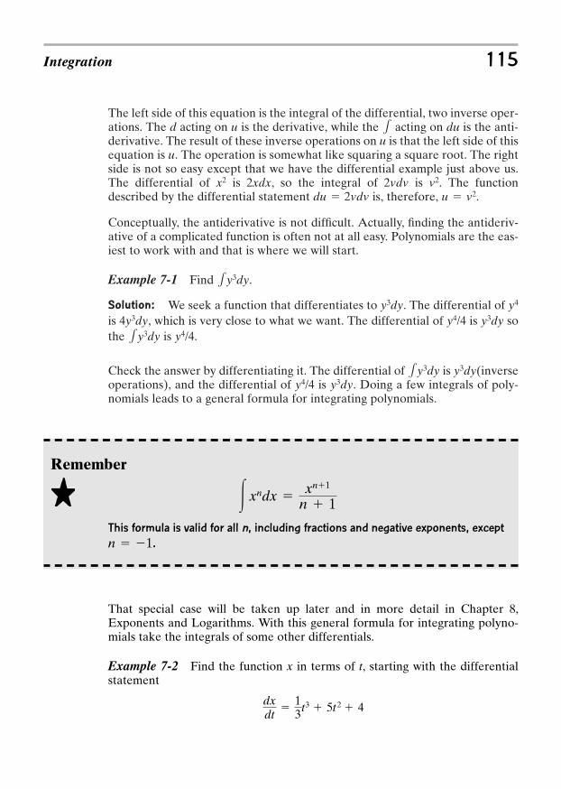
The left side of this equation is the integral of the differential, two inverse oper-ations. The d acting on u is the derivative, while the acting on du is the anti-derivative. The result of these inverse operations on u is that the left side of thisequation is u. The operation is somewhat like squaring a square root. The rightside is not so easy except that we have the differential example just above us.The differential of is , so the integral of is . The functiondescribed by the differential statement is, therefore, .
Conceptually, the antiderivative is not difficult. Actually, finding the antideriv-ative of a complicated function is often not at all easy. Polynomials are the eas-iest to work with and that is where we will start.
Example 7-1 Find .
Solution: We seek a function that differentiates to . The differential of is , which is very close to what we want. The differential of is sothe is .
Check the answer by differentiating it. The differential of is (inverseoperations), and the differential of is . Doing a few integrals of poly-nomials leads to a general formula for integrating polynomials.
y3dyy4/4y3dy1y3dy
y4/41y3dyy3dyy4/44y3dy
y4y3dy
1y3dy
u v2du 2vdvv22vdv2xdxx2
1
Integration 115
Remember
This formula is valid for all n, including fractions and negative exponents, except
.n 1
3 xndx xn1
n 1
That special case will be taken up later and in more detail in Chapter 8,Exponents and Logarithms. With this general formula for integrating polyno-mials take the integrals of some other differentials.
Example 7-2 Find the function x in terms of t, starting with the differentialstatement
dxdt
13t3 5t 2 4
Solution: First rewrite the problem as .
The integral of is x so write .
Most formal integral problems are presented in this form. Now perform theintegration term by term, the same way the differential was formed to producethis integral
Don’t forget that the integral of a constant times dt is the constant times t.
The antiderivative as described so far is not the complete story of antideriva-tives, as is illustrated in the next problem. Take a look at a simple function,
. The derivative is . Now take the antideriva-tive of .
and
Where did the 7 in the original function go? Differentiating the function pro-duced a zero for the 7. Integrating the with the antiderivative approachproduced the terms but not the 7. Given an integral problem as
the integral of is and the integral of is but it is impossible todetermine if there is a constant in the expression for y.
The correct solution to this integral is: .y 1(2x 2)dx x2 2x C
2x2dxx22xdx
y 3 (2x 2)dx
x2 2x2x 2
y 3 (2x 2)dx 2x2
2 2x x2 2xdy (2x 2)dx
2x 2dy/dx 2x 2y x2 2x 7
x 13 Q
t 4
4 R 5Q t3
3 R 4t t 4
12
5t3
3 4t
x 3 Q13t3 5t2 4Rdtdx
dx Q13t3 5t2 4Rdt
116 CALCULUS FOR THE UTTERLY CONFUSED
Quick Tip
Integrals obtained by taking the antiderivative must be written with an arbitrary
constant. The constant can be determined if other details are specified in the prob-
lem. Integrals requiring a constant (of integration) are called indefinite integrals.
There is a way around this problem but for the time being just remember to include
the constant and evaluate it if possible from the information in the problem.
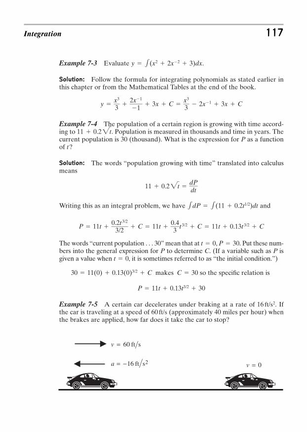
Example 7-3 Evaluate .
Solution: Follow the formula for integrating polynomials as stated earlier inthis chapter or from the Mathematical Tables at the end of the book.
Example 7-4 The population of a certain region is growing with time accord-ing to . Population is measured in thousands and time in years. Thecurrent population is 30 (thousand). What is the expression for P as a functionof t?
Solution: The words “population growing with time” translated into calculusmeans
Writing this as an integral problem, we have and
The words “current population . . . 30” mean that at , . Put these num-bers into the general expression for P to determine C. (If a variable such as P isgiven a value when , it is sometimes referred to as “the initial condition.”)
makes so the specific relation is
Example 7-5 A certain car decelerates under braking at a rate of . Ifthe car is traveling at a speed of (approximately 40 miles per hour) whenthe brakes are applied, how far does it take the car to stop?
60 ft/s16 ft/s2
P 11t 0.13t3/2 30
C 3030 11(0) 0.13(0)3/2 C
t 0
P 30t 0
P 11t 0.2t 3/2
3/2 C 11t
0.43 t 3/2 C 11t 0.13t 3/2 C
1dP 1(11 0.2t1/2)dt
11 0.22t dPdt
11 0.22t
y x3
3 2x1
1 3x C
x3
3 2x1 3x C
y 1(x2 2x2 3)dx
Integration 117
sft60=v
2sft16= −a 0=v
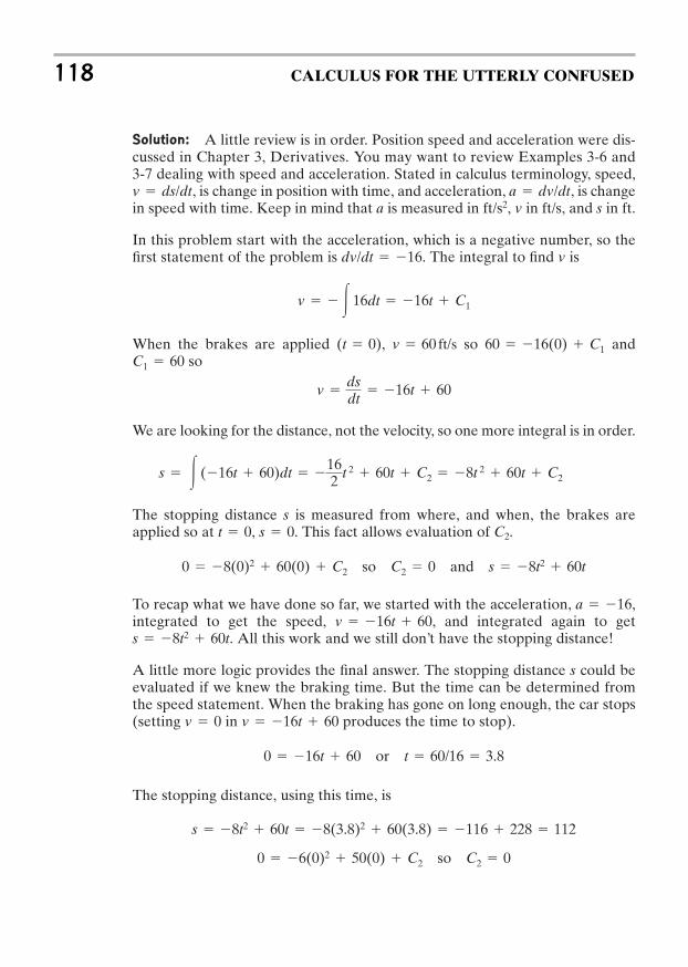
Solution: A little review is in order. Position speed and acceleration were dis-cussed in Chapter 3, Derivatives. You may want to review Examples 3-6 and3-7 dealing with speed and acceleration. Stated in calculus terminology, speed,
, is change in position with time, and acceleration, , is changein speed with time. Keep in mind that a is measured in ft/s2, v in ft/s, and s in ft.
In this problem start with the acceleration, which is a negative number, so thefirst statement of the problem is . The integral to find v is
When the brakes are applied , so andso
We are looking for the distance, not the velocity, so one more integral is in order.
The stopping distance s is measured from where, and when, the brakes areapplied so at , . This fact allows evaluation of C2.
so and
To recap what we have done so far, we started with the acceleration, ,integrated to get the speed, , and integrated again to get
All this work and we still don’t have the stopping distance!
A little more logic provides the final answer. The stopping distance s could beevaluated if we knew the braking time. But the time can be determined fromthe speed statement. When the braking has gone on long enough, the car stops(setting in produces the time to stop).
or
The stopping distance, using this time, is
so C2 00 6(0)2 50(0) C2
s 8t2 60t 8(3.8)2 60(3.8) 116 228 112
t 60/16 3.80 16t 60
v 16t 60v 0
s 8t2 60t.v 16t 60
a 16
s 8t2 60tC2 00 8(0)2 60(0) C2
s 0t 0
s 3 (16t 60)dt 162 t 2 60t C2 8t 2 60t C2
v dsdt
16t 60
C1 6060 16(0) C1v 60 ft/s(t 0)
v 3 16dt 16t C1
dv/dt 16
a dv/dtv ds/dt
118 CALCULUS FOR THE UTTERLY CONFUSED

The problems so far have been in the form y equals the integral of some poly-nomial in x times dx. The next problem illustrates a type of problem where thederivative depends on both variables.
Example 7-6 The rate of change of a certain variable x with y is equal to thesquare root of the product of x and y. Find y as a function of x.
This is a problem where the words prescribe the mathematics. The phrase “therate of change of . . . x with y” means derivative; the phrase “the square root ofthe product” is clear. Form the product and take the square root. Read the sen-tence carefully, several times if necessary, and write
With the problem written down, another difficulty appears. This is not a sim-ple dy equals a polynomial times dx problem. Separating the variables isgoing to take a little work. With a little manipulation the statement can bewritten as
This process is called separating the variables. While this problem is a little dif-ferent from previous problems neither integral is difficult.
or
Perform each integration, and with a little algebra x . . . or
y . . . can be written as or or
or
Notice that instead of writing C/2, a new constant C1 was introduced. If at theend of the problem the constant is evaluated it does not matter whether theconstant is two times the original or any other multiple or root, or whatever ofthe original. Also notice that C2 is a new constant.
y [3x1/2 C2]2/3
y3/2 3x1/2 C2x Sy3/2
3 C1T2
x1/2 y3/2
3 C1
x1/2
1/2
y3/2
3/2 C
3 x1/2dx 3 y1/2dyx1/2dx y1/2dy
dx
2x 2ydy
dxdy
2xy
Integration 119
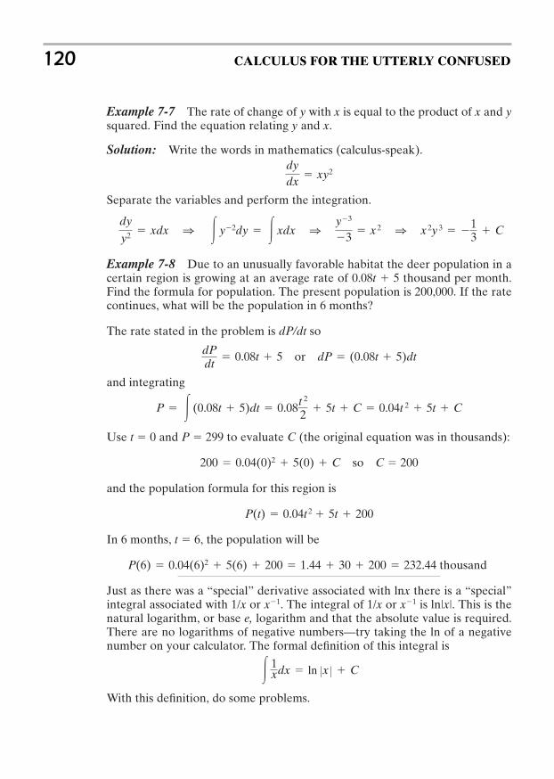
Example 7-7 The rate of change of y with x is equal to the product of x and ysquared. Find the equation relating y and x.
Solution: Write the words in mathematics (calculus-speak).
Separate the variables and perform the integration.
Example 7-8 Due to an unusually favorable habitat the deer population in acertain region is growing at an average rate of 0.08t 5 thousand per month.Find the formula for population. The present population is 200,000. If the ratecontinues, what will be the population in 6 months?
The rate stated in the problem is dP/dt so
or
and integrating
Use t 0 and P 299 to evaluate C (the original equation was in thousands):
so C 200
and the population formula for this region is
In 6 months, t 6, the population will be
Just as there was a “special” derivative associated with lnx there is a “special”integral associated with 1/x or x1. The integral of 1/x or x1 is ln|x|. This is thenatural logarithm, or base e, logarithm and that the absolute value is required.There are no logarithms of negative numbers—try taking the ln of a negativenumber on your calculator. The formal definition of this integral is
With this definition, do some problems.
3 1xdx ln Zx Z C
P(6) 0.04(6)2 5(6) 200 1.44 30 200 232.44 thousand
P(t) 0.04t 2 5t 200
200 0.04(0)2 5(0) C
P 3 (0.08t 5)dt 0.08t 2
2 5t C 0.04t 2 5t C
dP (0.08t 5)dtdPdt
0.08t 5
dy
y2 xdx 1 3 y2dy 3 xdx 1 y3
3 x 2 1 x 2y 3 13 C
dydx
xy2
120 CALCULUS FOR THE UTTERLY CONFUSED
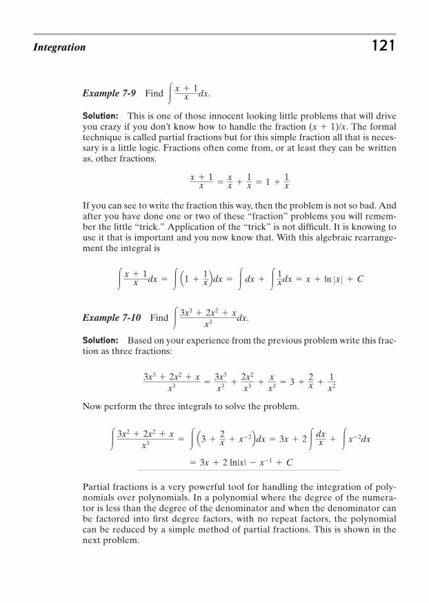
Example 7-9 Find .
Solution: This is one of those innocent looking little problems that will driveyou crazy if you don’t know how to handle the fraction (x 1)/x. The formaltechnique is called partial fractions but for this simple fraction all that is neces-sary is a little logic. Fractions often come from, or at least they can be writtenas, other fractions.
If you can see to write the fraction this way, then the problem is not so bad. Andafter you have done one or two of these “fraction” problems you will remem-ber the little “trick.” Application of the “trick” is not difficult. It is knowing touse it that is important and you now know that. With this algebraic rearrange-ment the integral is
Example 7-10 Find .
Solution: Based on your experience from the previous problem write this frac-tion as three fractions:
Now perform the three integrals to solve the problem.
Partial fractions is a very powerful tool for handling the integration of poly-nomials over polynomials. In a polynomial where the degree of the numera-tor is less than the degree of the denominator and when the denominator canbe factored into first degree factors, with no repeat factors, the polynomialcan be reduced by a simple method of partial fractions. This is shown in thenext problem.
3x 2 ln|x| x1 C
3 3x2 2x2 xx3 3 Q3
2x x2Rdx 3x 2 3 dx
x 3 x2dx
3x3 2x2 xx3
3x3
x3 2x2
x3 xx3 3
2x
1x2
3 3x3 2x2 xx3 dx
3 x 1x dx 3 Q1
1xRdx 3 dx 3 1
xdx x ln Zx Z C
x 1x
xx
1x 1
1x
3 x 1x dx
Integration 121
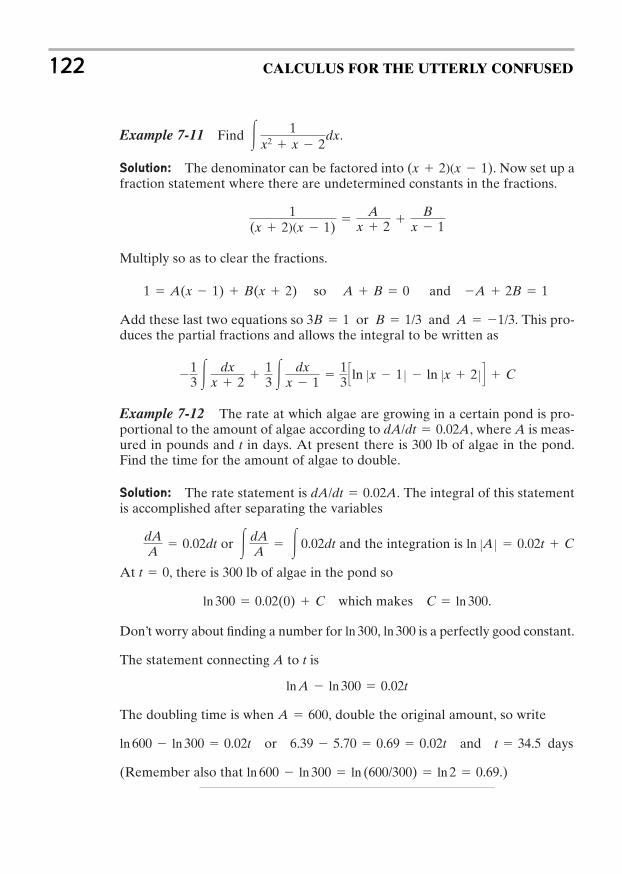
Example 7-11 Find .
Solution: The denominator can be factored into . Now set up afraction statement where there are undetermined constants in the fractions.
Multiply so as to clear the fractions.
Add these last two equations so . This pro-duces the partial fractions and allows the integral to be written as
Example 7-12 The rate at which algae are growing in a certain pond is pro-portional to the amount of algae according to , where A is meas-ured in pounds and t in days. At present there is 300 lb of algae in the pond.Find the time for the amount of algae to double.
Solution: The rate statement is . The integral of this statementis accomplished after separating the variables
or and the integration is
At , there is 300 lb of algae in the pond so
which makes .
Don’t worry about finding a number for , is a perfectly good constant.
The statement connecting A to t is
The doubling time is when , double the original amount, so write
or and days
(Remember also that .)ln 600 ln 300 ln (600/300) ln 2 0.69
t 34.56.39 5.70 0.69 0.02tln 600 ln 300 0.02t
A 600
ln A ln 300 0.02t
ln 300ln 300
C ln 300ln 300 0.02(0) C
t 0
ln ZA Z 0.02t C3 dAA
3 0.02dtdAA
0.02dt
dA/dt 0.02A
dA/dt 0.02A
13 3 dx
x 2 13 3 dx
x 1
13 Sln Zx 1 Z ln Zx 2 Z T C
3B 1 or B 1/3 and A 1/3
1 A(x 1) B(x 2) so A B 0 and A 2B 1
1(x 2)(x 1)
A
x 2 B
x 1
(x 2)(x 1)
3 1x2 x 2
dx
122 CALCULUS FOR THE UTTERLY CONFUSED
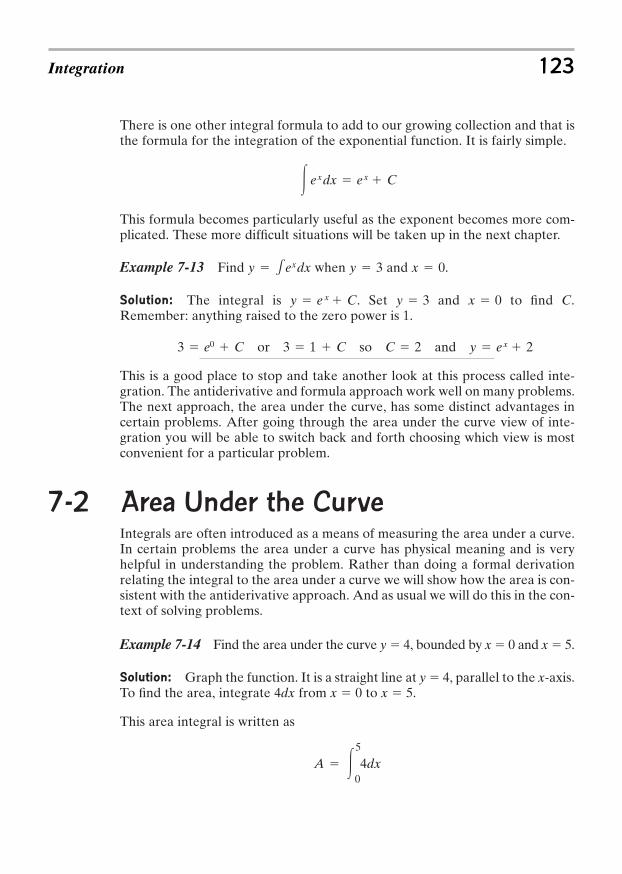
There is one other integral formula to add to our growing collection and that isthe formula for the integration of the exponential function. It is fairly simple.
This formula becomes particularly useful as the exponent becomes more com-plicated. These more difficult situations will be taken up in the next chapter.
Example 7-13 Find when and .
Solution: The integral is . Set and to find C.Remember: anything raised to the zero power is 1.
or so and
This is a good place to stop and take another look at this process called inte-gration. The antiderivative and formula approach work well on many problems.The next approach, the area under the curve, has some distinct advantages incertain problems. After going through the area under the curve view of inte-gration you will be able to switch back and forth choosing which view is mostconvenient for a particular problem.
7-2 Area Under the CurveIntegrals are often introduced as a means of measuring the area under a curve.In certain problems the area under a curve has physical meaning and is veryhelpful in understanding the problem. Rather than doing a formal derivationrelating the integral to the area under a curve we will show how the area is con-sistent with the antiderivative approach. And as usual we will do this in the con-text of solving problems.
Example 7-14 Find the area under the curve y 4, bounded by x 0 and x 5.
Solution: Graph the function. It is a straight line at y 4, parallel to the x-axis.To find the area, integrate 4dx from x 0 to x 5.
This area integral is written as
A 35
04dx
y ex 2C 23 1 C3 e0 C
x 0y 3y e x C
x 0y 3y 1exdx
3 exdx ex C
Integration 123
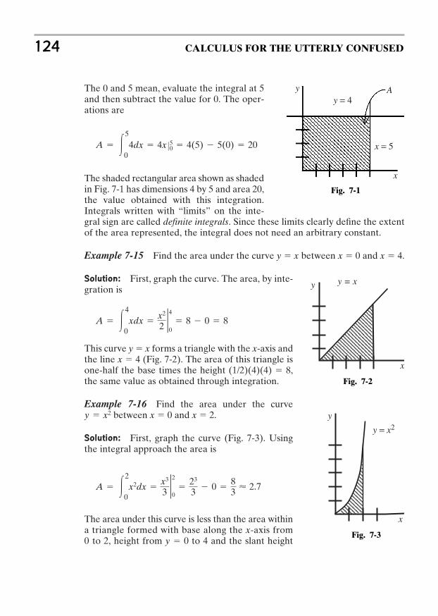
The 0 and 5 mean, evaluate the integral at 5and then subtract the value for 0. The oper-ations are
The shaded rectangular area shown as shadedin Fig. 7-1 has dimensions 4 by 5 and area 20,the value obtained with this integration.Integrals written with “limits” on the inte-gral sign are called definite integrals. Since these limits clearly define the extentof the area represented, the integral does not need an arbitrary constant.
Example 7-15 Find the area under the curve y x between x 0 and x 4.
Solution: First, graph the curve. The area, by inte-gration is
This curve y x forms a triangle with the x-axis andthe line x 4 (Fig. 7-2). The area of this triangle isone-half the base times the height (1/2)(4)(4) 8,the same value as obtained through integration.
Example 7-16 Find the area under the curvebetween x 0 and x 2.
Solution: First, graph the curve (Fig. 7-3). Usingthe integral approach the area is
The area under this curve is less than the area withina triangle formed with base along the x-axis from0 to 2, height from y 0 to 4 and the slant height
A 32
0x2dx
x3
32 20
23
3 0 83 < 2.7
y x2
A 34
0xdx
x2
22 40
8 0 8
A 35
04dx 4x Z50 4(5) 5(0) 20
124 CALCULUS FOR THE UTTERLY CONFUSED
y = 4y
x = 5
x
A
Fig. 7-1
Fig. 7-2
y
x
y = x
Fig. 7-3
y = x2
y
x
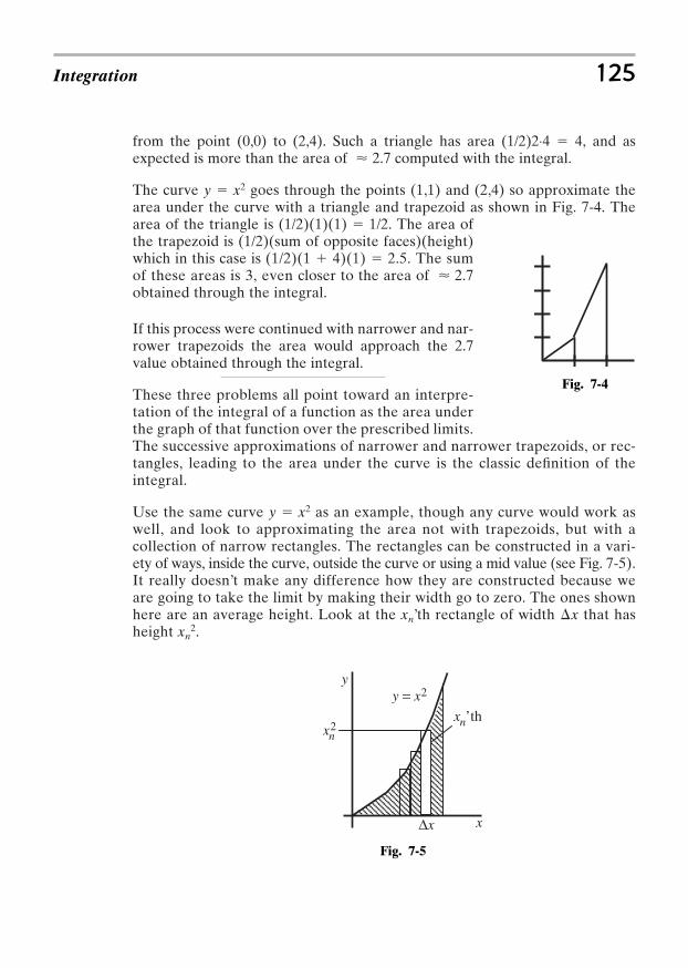
from the point (0,0) to (2,4). Such a triangle has area (1/2)2⋅4 4, and asexpected is more than the area of 2.7 computed with the integral.
The curve goes through the points (1,1) and (2,4) so approximate thearea under the curve with a triangle and trapezoid as shown in Fig. 7-4. Thearea of the triangle is (1/2)(1)(1) 1/2. The area ofthe trapezoid is (1/2)(sum of opposite faces)(height)which in this case is (1/2)(1 4)(1) 2.5. The sumof these areas is 3, even closer to the area of 2.7obtained through the integral.
If this process were continued with narrower and nar-rower trapezoids the area would approach the 2.7value obtained through the integral.
These three problems all point toward an interpre-tation of the integral of a function as the area underthe graph of that function over the prescribed limits.The successive approximations of narrower and narrower trapezoids, or rec-tangles, leading to the area under the curve is the classic definition of theintegral.
Use the same curve as an example, though any curve would work aswell, and look to approximating the area not with trapezoids, but with acollection of narrow rectangles. The rectangles can be constructed in a vari-ety of ways, inside the curve, outside the curve or using a mid value (see Fig. 7-5).It really doesn’t make any difference how they are constructed because weare going to take the limit by making their width go to zero. The ones shownhere are an average height. Look at the xn’th rectangle of width that hasheight xn
2. x
y x2
<
y x2
<
Integration 125
Fig. 7-5
2nx
nx ’th
∆x
2y = xy
x
Fig. 7-4
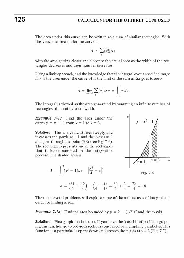
The area under this curve can be written as a sum of similar rectangles. Withthis view, the area under the curve is
with the area getting closer and closer to the actual area as the width of the rec-tangles decreases and their number increases.
Using a limit approach, and the knowledge that the integral over a specified rangein x is the area under the curve, A is the limit of the sum as goes to zero.
The integral is viewed as the area generated by summing an infinite number ofrectangles of infinitely small width.
Example 7-17 Find the area under thecurve from x 1 to x 3.
Solution: This is a cubic. It rises steeply, andit crosses the y-axis at 1 and the x-axis at 1and goes through the point (3,8) (see Fig. 7-6).The rectangle represents one of the rectanglesthat is being summed in the integrationprocess. The shaded area is
The next several problems will explore some of the unique uses of integral cal-culus for finding areas.
Example 7-18 Find the area bounded by and the x-axis.
Solution: First graph the function. If you have the least bit of problem graph-ing this function go to previous sections concerned with graphing parabolas. Thisfunction is a parabola. It opens down and crosses the y-axis at y = 2 (Fig. 7-7).
y 2 (1/2)x2
A Q814
124 R Q
14
44R
694
34
724 18
A 33
1(x3 1)dx S
x4
4 xT3
1
y x3 1
A lim xS0an (x2
n) x 3x
0x2dx
x
A < an
(x2n) x
126 CALCULUS FOR THE UTTERLY CONFUSED
Fig. 7-6
y
x
3y = x
x = 3x = 1
− 1
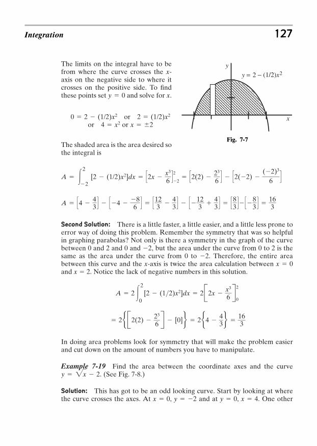
The limits on the integral have to befrom where the curve crosses the x-axis on the negative side to where itcrosses on the positive side. To findthese points set and solve for x.
oror or
The shaded area is the area desired sothe integral is
Second Solution: There is a little faster, a little easier, and a little less prone toerror way of doing this problem. Remember the symmetry that was so helpfulin graphing parabolas? Not only is there a symmetry in the graph of the curvebetween 0 and 2 and 0 and 2, but the area under the curve from 0 to 2 is thesame as the area under the curve from 0 to 2. Therefore, the entire areabetween this curve and the x-axis is twice the area calculation between x 0and x 2. Notice the lack of negative numbers in this solution.
In doing area problems look for symmetry that will make the problem easierand cut down on the amount of numbers you have to manipulate.
Example 7-19 Find the area between the coordinate axes and the curve. (See Fig. 7-8.)
Solution: This has got to be an odd looking curve. Start by looking at wherethe curve crosses the axes. At x 0, y 2 and at y 0, x 4. One other
y 2x 2
2b B2(2) 23
6R [0]r 2b4
43 r
163
A 2 32
0[2 (1>2)x2]dx 2B2x
x3
6R 2
0
A S4 43 T S4
86T S
123
43 T S
123
43 T S
83 T S
83 T
163
A 32
2[2 (1/2)x2]dx S2x
x3
6T2
2 S2(2)
23
6T S2(2)
(2)3
6T
x 24 x22 (1/2)x20 2 (1/2)x2
y 0
Integration 127
Fig. 7-7
2 (1/2)xy = 2 −y
x
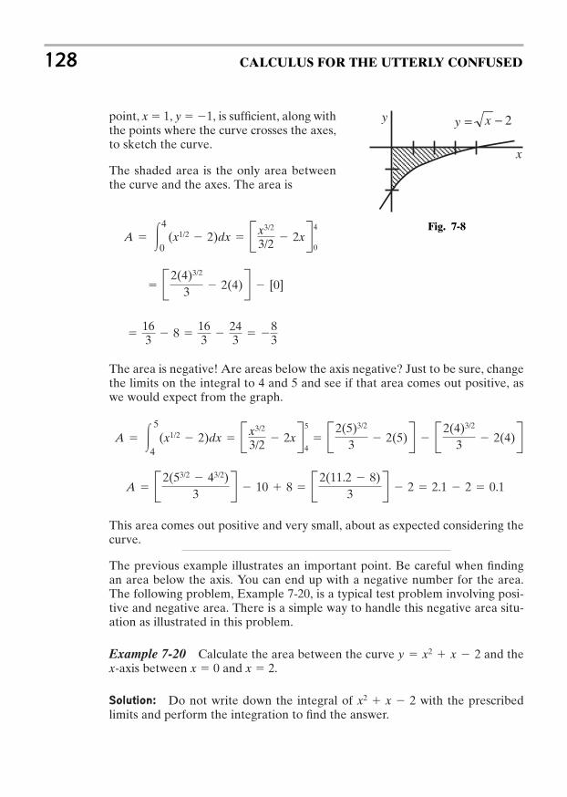
point, x 1, y 1, is sufficient, along withthe points where the curve crosses the axes,to sketch the curve.
The shaded area is the only area betweenthe curve and the axes. The area is
The area is negative! Are areas below the axis negative? Just to be sure, changethe limits on the integral to 4 and 5 and see if that area comes out positive, aswe would expect from the graph.
This area comes out positive and very small, about as expected considering thecurve.
The previous example illustrates an important point. Be careful when findingan area below the axis. You can end up with a negative number for the area.The following problem, Example 7-20, is a typical test problem involving posi-tive and negative area. There is a simple way to handle this negative area situ-ation as illustrated in this problem.
Example 7-20 Calculate the area between the curve and thex-axis between x 0 and x 2.
Solution: Do not write down the integral of with the prescribedlimits and perform the integration to find the answer.
x2 x 2
y x2 x 2
A B2(53/2 43/2)3 R 10 8 B2(11.2 8)
3 R 2 2.1 2 0.1
A 35
4(x1/2 2)dx Bx3/2
3/2 2xR 5
4 B2(5)3/2
3 2(5)R B2(4)3/2
3 2(4)R
163 8
163
243
83
B2(4)3/2
3 2(4)R [0]
A 34
0(x1/2 2)dx Bx3/2
3/2 2xR 4
0
128 CALCULUS FOR THE UTTERLY CONFUSED
Fig. 7-8
y
x
2= x -y
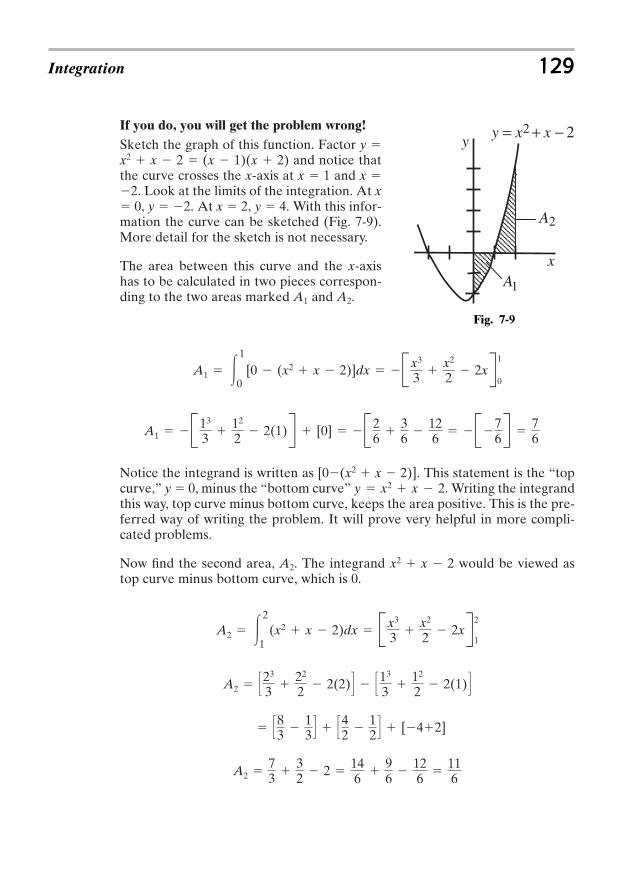
If you do, you will get the problem wrong!Sketch the graph of this function. Factor y x2 x 2 (x 1)(x 2) and notice thatthe curve crosses the x-axis at x 1 and x 2. Look at the limits of the integration. At x 0, y 2. At x 2, y 4. With this infor-mation the curve can be sketched (Fig. 7-9).More detail for the sketch is not necessary.
The area between this curve and the x-axishas to be calculated in two pieces correspon-ding to the two areas marked A1 and A2.
Notice the integrand is written as [0(x2 x 2)]. This statement is the “topcurve,” y 0, minus the “bottom curve” . Writing the integrandthis way, top curve minus bottom curve, keeps the area positive. This is the pre-ferred way of writing the problem. It will prove very helpful in more compli-cated problems.
Now find the second area, A2. The integrand would be viewed astop curve minus bottom curve, which is 0.
A2 73
32 2
146
96
126
116
S83
13 T S
42
12 T [42]
A2 S23
3 22
2 2(2)T S13
3 12
2 2(1)T
A2 32
1(x2 x 2)dx Bx3
3 x2
2 2xR 2
1
x2 x 2
y x2 x 2
A1 B13
3 12
2 2(1)R [0] B26
36
126
B76R
76
A1 31
0[0 (x2 x 2)]dx Bx3
3 x2
2 2xR 1
0
Integration 129
Fig. 7-9
22 += x −xy
x
1A
2A
y
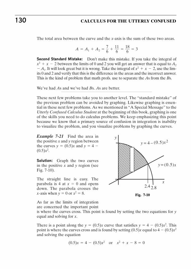
The total area between the curve and the x-axis is the sum of these two areas.
Second Standard Mistake: Don’t make this mistake. If you take the integral ofbetween the limits of 0 and 2 you will get an answer that is equal to A2
A1. It will look great but it is wrong. Take the integral of , use the lim-its 0 and 2 and verify that this is the difference in the areas and the incorrect answer.This is the kind of problem that math profs. use to separate the As from the Bs.
We’ve had As and we’ve had Bs. As are better.
These next few problems take you to another level. The “standard mistake” ofthe previous problem can be avoided by graphing. Likewise graphing is essen-tial in these next few problems. As we mentioned in “A Special Message” to theUtterly Confused Calculus Student at the beginning of this book, graphing is oneof the skills you need to do calculus problems. We keep emphasizing this pointbecause we know that a primary source of confusion in integration is inabilityto visualize the problem, and you visualize problems by graphing the curves.
Example 7-21 Find the area inthe positive x and y region betweenthe curves and y 4 (0.5)x2.
Solution: Graph the two curvesin the positive x and y region (seeFig. 7-10).
The straight line is easy. Theparabola is 4 at x 0 and opensdown. The parabola crosses thex-axis when y 0 or x2 8.
As far as the limits of integrationare concerned the important pointis where the curves cross. This point is found by setting the two equations for yequal and solving for x.
There is a point along the y (0.5)x curve that satisfies y 4 (0.5)x2. Thispoint is where the curves cross and is found by setting (0.5)x equal to 4 (0.5)x2
and solving the equation
or x2 x 8 0(0.5)x 4 (0.5)x2
y (0.5)x
x2 x 2x2 x 2
A A1 A2 76
116
186
3
130 CALCULUS FOR THE UTTERLY CONFUSED
Fig. 7-10
2.4 2.8
y
x
xy )5.0(=
2)5.0( xy = 4 _
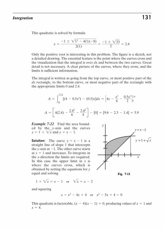
This quadratic is solved by formula
Only the positive root is interesting in this problem. The figure is a sketch, nota detailed drawing. The essential feature is the point where the curves cross andthe visualization that the integral is over dx and between the two curves. Greatdetail is not necessary. A clear picture of the curves, where they cross, and thelimits is sufficient information.
The integral is written as going from the top curve, or most positive part of thedx rectangle, to the bottom curve, or most negative part of the rectangle withthe appropriate limits 0 and 2.4.
Example 7-22 Find the area bound-ed by the y-axis and the curves
and .
Solution: The curve is astraight line of slope 1 that interceptsthe y-axis at 1. The other curve startsat and increases. To integrate inthe x-direction the limits are required.In this case the upper limit in x iswhere the curves cross, which isobtained by setting the equations for yequal and solving
and squaring
This quadratic is factorable, , producing values of and.x 4
x 1(x 4)(x 1) 0
x x2 4x 4 or x2 5x 4 0
1 2x x 1 or 2x x 2
y 1
y x 1
y x 1y 1 2x
A B4(2.4) 2.43
6
2.42
4 R [0] [9.6 2.3 1.4] 5.9
A 32.4
0[(4 0.5x2) (0.5)x]dx S4x
x3
6
0.5x2
2 T2.4
0
x 1 212 4(1)(8)
2(1)
1 2332 2.4
Integration 131
Fig. 7-11
xy +
−
= 1
1= xyy
x

The value requires a negative square root to work in both original equa-tions and is seen from Fig. 7-11 as incorrect. The value x 4 is the correct limitvalue. The x 1 point is a spurious one caused by squaring a square root andthen factoring the resulting equation. With the limits, set up the integral from0 to 4 of the upper curve minus the lower curve and integrate.
The next two problems are practical problems illustrating how calculus can helpin forecasting revenue generation in the one instance, and yield from a miningoperation in the other instance. The unique aspect of these problems is thatthey start not with a statement of revenue, but with a statement of revenue rate,the revenue generated per year and the yield of the mine in tons per year.Watch the way these problems are worded. Don’t be fooled on a test by mis-reading a rate statement.
Example 7-23 A certain machine generates revenue at the rate of, where R is in dollars per year and t is in years. As the machine
ages the cost of repairs increases according to: C(t) 500 2t2. How long is themachine profitable and what are the total earnings to this point in time?
Solution: The two curves are both parabolas, the R(t) curve opening downand the C(t) curve opening up. The curves are sketched here (Fig. 7-12). Detail isnot necessary.
R(t) 2000 5t2
A B2(4) 43/2
3/2
42
2 R B8 23(8) 8R
163
A 34
0[(1 2x) (x 1)]dx 3
4
0(2 x1/2 x)dx B2x
x3/2
3/2
x2
2R 4
0
x 1
132 CALCULUS FOR THE UTTERLY CONFUSED
Fig. 7-12
R (t) = 2000 5t 2
t
Rateof $
14.6
C (t) = 500 + 2t2
_
When the revenue generated per year equals the cost of repairs per year themachine stops being profitable.
Mathematically, this situation occurs when the curves cross. The time when theycross is found by setting the equations equal and solving for the time.
The total earnings up to 14.6 years is the (revenue generated) area under theR(t) curve minus the (cost) area under the C(t) curve. This is an integral. Lookat the units. The rate of return in dollars per year times the time is the totalnumber of dollars.
The total earnings until the machine becomes unprofitable, that is, costs moreto operate each year than it returns in revenue, is $14,638.
Example 7-24 In a mine the yield per unit costfor a particular ore is declining according to
, where the yield is in millions of tonsper year and t is in years. Find the time for the mineto produce 60 million tons of ore.
Solution: Be careful with rate statements like thisone. The yield equation is in millions of tons peryear, not millions of tons total. Since the yield is inmillions of tons per year, the time for 60 million tonshas to come from an integration over time.Integration is required rather than multiplicationbecause the rate per year is changing. The total yieldthen is
T 3t
0(8 0.4t)dt B8t
0.4t2
2 R t
0 8t 0.2t2
Y 8 0.4t
E B1500t 7t 3
3 R 14.6
0 1500(14.6)
7(14.6)3
3 21900 7262 14,638
E 314.6
0[(2000 5t 2) (500 2t 2)]dt 3
14.6
0[1500 7t 2 ]dt
15007 t 2 or t
Å1500
7 14.6 years
2000 5t2 500 2t2 or 1500 7t2
Integration 133
Notice that in this problem the limits are 0 and t because we are looking for thetime to produce a total of 60 (million tons). Therefore, set in the equation
generated by the integral and solve for the time.
or or
This quadratic is factorable to producing time values of10 and 30.
Go back to the original statement for the yield and note that atthe yield is and at the yield is
.
The 10 year figure is the realistic one. Who would work the mine until the yieldreached zero and then continue, putting ore back, until the 60 million total wasachieved?
Further Insight Solution: If the yield is then in 10 years the yieldgoes from 8 (starting at zero time) to in a linear fashion so the aver-age yield over the 10 years is 6. This 6 million tons per year average times the10 years produces the 60 million tons.
The 30 year figure is also true. If the yield goes according to for30 years then the yield goes from 8 at time zero to 4 at the end of 30 yearsand the average is 2 million tons per year for 30 years for the 60 million tontotal.
No one would actually do this because when the yield went to zero you wouldhave to start putting ore back into the mine to achieve your 60 million tonstotal! You would also expect the yield equation to not accurately represent themine production after the production rate had gone to zero.
Sometimes, in problems involving quadratics, solutions are generated that aremathematically correct but unrealistic. It is good practice to always look at theanswer and ask if it is reasonable.
Example 7-25 A demographic study indicates that the population of a certaintown is growing at the rate of people per month, when x is measuredin months. What will be the increase in population between the 10th and 12thmonths?
4 2x0.8
Y 8 0.4t
8 4 4Y 8 0.4t
Y(30) 8 0.4(30) 8 12 4t 30Y(10) 8 0.4(10) 4t 10
Y 8 0.4t
(t 10)(t 30) 0
t2 40t 300 00.2t2 8t 60 060 8t 0.2t2
T 8t 0.2t2
T 60
134 CALCULUS FOR THE UTTERLY CONFUSED
Solution: This is an integral problem. The growth function has to be integratedand evaluated at the 10th and 12th months. Write the integral as the number( ) and use the growth function integrated over time.
Before going any further review how to take a fractional power with your cal-culator. To find enter 12 on your calculator, then find a key that raises“things” to a power (this key will look like or ) and press it. Your calcula-tor will probably blink and continue to display the 12. That’s OK. Don’t worryabout the 12, enter 1.8, and press the equal sign. The calculator should take ashort time to display 88.
A total of 36 people will enter the town in the 10th to 12th month interval.
Example 7-26 A rare stamp is, and has been, appreci-ating at the rate of in thousands of dollars peryear when t is measured in years. If this stamp is pur-chased for $5000 for a newborn child and allowed toappreciate, what will be the value of the stamp on thechild’s 18th birthday?
Solution: This is a rate problem and an integral is required. The stamp is pur-chased (at ) for $5000. Integrate the rate over time with the limits of 0 and18 to find the value after 18 years.
In 18 years the stamp will be worth $171,000.
7-3 Average Value of a FunctionIntegral calculus can be used to determine the average values of functions. Theaverage value of some quantity that may be varying in a very complicated way
V 318
0(5 0.5t)dt B5t
0.5t2
2R 18
0 B5(18)
0.5(18)2
2R [90 81] 171
t 0
5 0.5t
N(10 12) B48 2(88)
1.8R B40
2(63)1.8
R [48 98] [40 70] 36
xyyx(12)1.8
N(10 12) B4(12) 2(12)1.8
1.8R B4(10)
2(10)1.8
1.8R
N(10 12) 312
10(4 2x 0.8 )dx B4x
2x1.8
1.8R 12
10
10 12
Integration 135
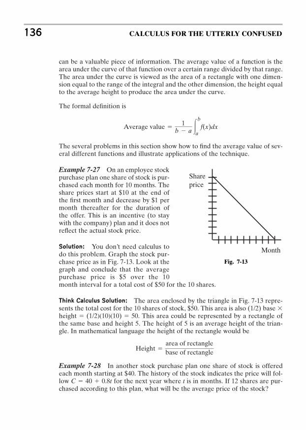
can be a valuable piece of information. The average value of a function is thearea under the curve of that function over a certain range divided by that range.The area under the curve is viewed as the area of a rectangle with one dimen-sion equal to the range of the integral and the other dimension, the height equalto the average height to produce the area under the curve.
The formal definition is
The several problems in this section show how to find the average value of sev-eral different functions and illustrate applications of the technique.
Example 7-27 On an employee stockpurchase plan one share of stock is pur-chased each month for 10 months. Theshare prices start at $10 at the end ofthe first month and decrease by $1 permonth thereafter for the duration ofthe offer. This is an incentive (to staywith the company) plan and it does notreflect the actual stock price.
Solution: You don’t need calculus todo this problem. Graph the stock pur-chase price as in Fig. 7-13. Look at thegraph and conclude that the averagepurchase price is $5 over the 10month interval for a total cost of $50 for the 10 shares.
Think Calculus Solution: The area enclosed by the triangle in Fig. 7-13 repre-sents the total cost for the 10 shares of stock, $50. This area is also (1/2) base height . This area could be represented by a rectangle ofthe same base and height 5. The height of 5 is an average height of the trian-gle. In mathematical language the height of the rectangle would be
Example 7-28 In another stock purchase plan one share of stock is offeredeach month starting at $40. The history of the stock indicates the price will fol-low for the next year where t is in months. If 12 shares are pur-chased according to this plan, what will be the average price of the stock?
C 40 0.8t
Height area of rectanglebase of rectangle
(1/2)(10)(10) 50
Average value 1
b a 3b
af(x)dx
136 CALCULUS FOR THE UTTERLY CONFUSED
Fig. 7-13
Shareprice
Month

Solution: Graph the price of the stock as shown inFig 7-14. The area under the curve is the total cost forthe 12 shares. This (total cost) area divided by 12, thebase of the rectangle with area equivalent to this totalcost, gives the average price of the stock.
Integration 137
Following the form of integral stated earlier we calculate
The average price of the stock will be $44.80.
The average-value-of-a-function problems so far have had pretty tame-lookingfunctions. This next problem will illustrate how to apply the average value of afunction to some more complex functions.
Cavg 112
[480 57.6] 44.8
Cavg B40(12) (0.8)(12)2
2 R
Cavg 112B40t
0.8t2
2 R 12
0
Cavg 1
12 0 312
0(40 0.8t)dt
1 Share
Fig. 7-14
Cost pershare tC 8.040 +=
12Time
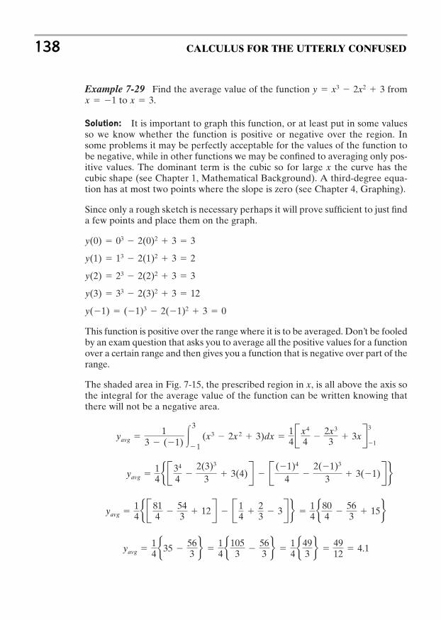
Example 7-29 Find the average value of the function fromto .
Solution: It is important to graph this function, or at least put in some valuesso we know whether the function is positive or negative over the region. Insome problems it may be perfectly acceptable for the values of the function tobe negative, while in other functions we may be confined to averaging only pos-itive values. The dominant term is the cubic so for large x the curve has thecubic shape (see Chapter 1, Mathematical Background). A third-degree equa-tion has at most two points where the slope is zero (see Chapter 4, Graphing).
Since only a rough sketch is necessary perhaps it will prove sufficient to just finda few points and place them on the graph.
This function is positive over the range where it is to be averaged. Don’t be fooledby an exam question that asks you to average all the positive values for a functionover a certain range and then gives you a function that is negative over part of therange.
The shaded area in Fig. 7-15, the prescribed region in x, is all above the axis sothe integral for the average value of the function can be written knowing thatthere will not be a negative area.
yavg 14 b35
563 r
14 b105
3 563 r
14 b49
3 r 4912
4.1
yavg 14 b B 81
4 543 12R B1
4 23 3R r
14 b80
4 563 15r
yavg 14 b B34
4 2(3)3
3 3(4)R B (1)4
4 2(1)3
3 3(1)R r
yavg 1
3 (1) 33
1(x3 2x 2 3)dx
14Bx4
4 2x3
3 3xR 3
1
y(1) (1)3 2(1)2 3 0
y(3) 33 2(3)2 3 12
y(2) 23 2(2)2 3 3
y(1) 13 2(1)2 3 2
y(0) 03 2(0)2 3 3
x 3x 1y x3 2x2 3
138 CALCULUS FOR THE UTTERLY CONFUSED
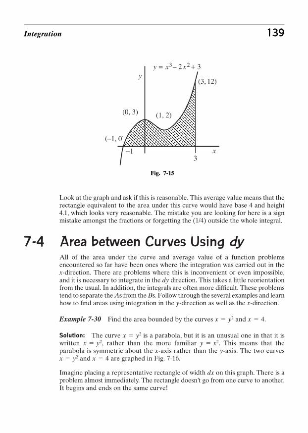
Look at the graph and ask if this is reasonable. This average value means that therectangle equivalent to the area under this curve would have base 4 and height4.1, which looks very reasonable. The mistake you are looking for here is a signmistake amongst the fractions or forgetting the (1/4) outside the whole integral.
7-4 Area between Curves Using dyAll of the area under the curve and average value of a function problemsencountered so far have been ones where the integration was carried out in thex-direction. There are problems where this is inconvenient or even impossible,and it is necessary to integrate in the dy direction. This takes a little reorientationfrom the usual. In addition, the integrals are often more difficult. These problemstend to separate the As from the Bs. Follow through the several examples and learnhow to find areas using integration in the y-direction as well as the x-direction.
Example 7-30 Find the area bounded by the curves and .
Solution: The curve is a parabola, but it is an unusual one in that it iswritten , rather than the more familiar . This means that theparabola is symmetric about the x-axis rather than the y-axis. The two curves
and are graphed in Fig. 7-16.
Imagine placing a representative rectangle of width dx on this graph. There is aproblem almost immediately. The rectangle doesn’t go from one curve to another.It begins and ends on the same curve!
x 4x y2
y x2x y2x y2
x 4x y2
Integration 139
Fig. 7-15
−1, 0)(
(3, 12)
(1, 2) (0, 3)
y32 23 += xxy
−13
x
_
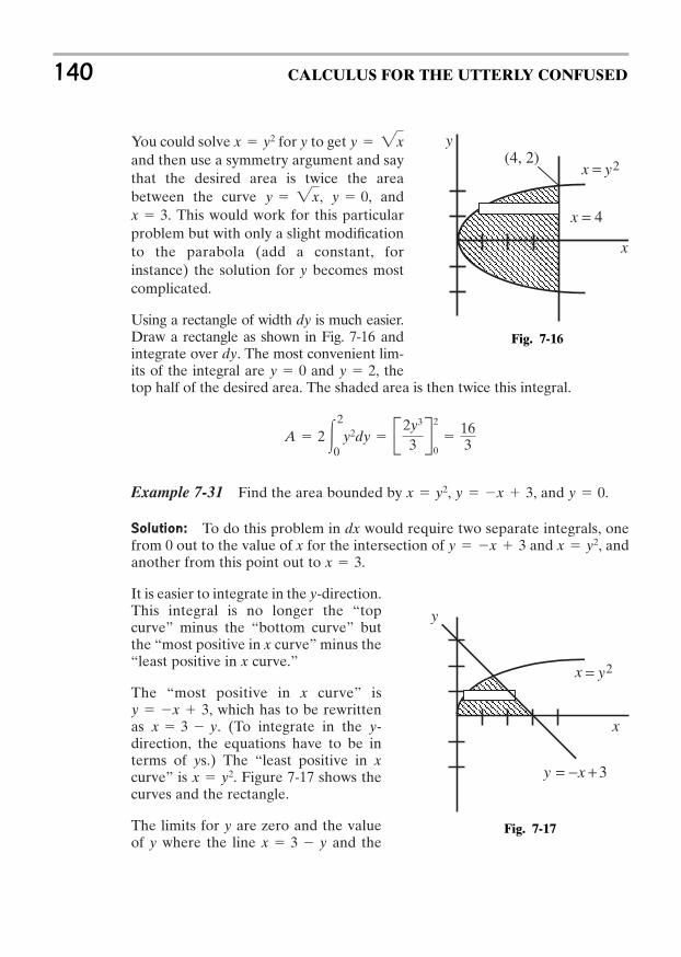
You could solve for y to get and then use a symmetry argument and saythat the desired area is twice the areabetween the curve , , and
. This would work for this particularproblem but with only a slight modificationto the parabola (add a constant, forinstance) the solution for y becomes mostcomplicated.
Using a rectangle of width dy is much easier.Draw a rectangle as shown in Fig. 7-16 andintegrate over dy. The most convenient lim-its of the integral are and , thetop half of the desired area. The shaded area is then twice this integral.
Example 7-31 Find the area bounded by , , and .
Solution: To do this problem in dx would require two separate integrals, onefrom 0 out to the value of x for the intersection of and , andanother from this point out to .
It is easier to integrate in the y-direction.This integral is no longer the “topcurve” minus the “bottom curve” butthe “most positive in x curve” minus the“least positive in x curve.”
The “most positive in x curve” is, which has to be rewritten
as . (To integrate in the y-direction, the equations have to be interms of ys.) The “least positive in xcurve” is . Figure 7-17 shows thecurves and the rectangle.
The limits for y are zero and the valueof y where the line and thex 3 y
x y2
x 3 yy x 3
x 3x y2y x 3
y 0y x 3x y2
A 2 32
0y2dy B2y3
3 R 2
0
163
y 2y 0
x 3y 0y 2x
y 2xx y2
140 CALCULUS FOR THE UTTERLY CONFUSED
Fig. 7-16
(4, 2) 2yx =
x = 4
x
y
Fig. 7-17
3+= −xy
2yx =
x
y
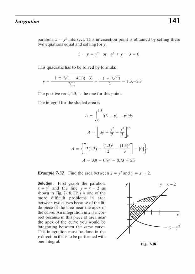
parabola intersect. This intersection point is obtained by setting thesetwo equations equal and solving for y.
or
This quadratic has to be solved by formula:
The positive root, 1.3, is the one for this point.
The integral for the shaded area is
Example 7-32 Find the area between and .
Solution: First graph the parabolaand the line as
shown in Fig. 7-18. This is one of themore difficult problems in areabetween two curves because of the lit-tle piece of the area near the apex ofthe curve. An integration in x is incor-rect because in this piece of area nearthe apex of the curve you would beintegrating between the same curve.This integration must be done in they-direction if it is to be performed withone integral.
y x 2x y2
y x 2x y2
A 3.9 0.84 0.73 2.3
A b B3(1.3) (1.3)2
2 (1.3)3
3 R [0]r
A B3y y2
2 y3
3 R1.3
0
A 31.3
0[(3 y) y2]dy
y 1 21 4(1)(3)
2(1)
1 2132 1.3,2.3
y2 y 3 03 y y2
x y2
Integration 141
Fig. 7-18
= x - 2y
2yx =
x
y
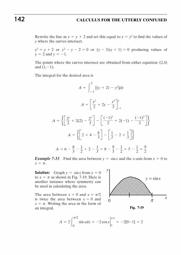
Rewrite the line as and set this equal to to find the values ofy where the curves intersect.
or or producing values ofand
The points where the curves intersect are obtained from either equation: (2,4)and .
The integral for the desired area is
Example 7-33 Find the area between and the x-axis from to.
Solution: Graph from to as shown in Fig. 7-19. Here isanother instance where symmetry canbe used in calculating the area.
The area between and is twice the area between and
. Writing the area in the form ofan integral,
A 2 3p/2
0sin xdx 2 cos x 2p/2
0 2[01] 2
x px 0
x p/2x 0
x px 0y sin x
x px 0y sin x
A 6 83
12 2
13 8
93
12 5
12
92
A b B2 4 83R B1
2 2 13R r
A b B22
2 2(2) 23
3 R B (1)2
2 2(1) (1)3
3 R r
A By2
2 2y y3
3 R2
1
A 32
1[(y 2) y2]dy
(1,1)
y 1.y 2(y 2)(y 1) 0y2 y 2 0y2 y 2
x y2x y 2
142 CALCULUS FOR THE UTTERLY CONFUSED
Fig. 7-19
0 p
y
x
xy sin=
The easiest way to verify this integral is to refer to the Mathematical Tables. Ifyou have any trouble recalling the shape of the cosine curve, check Chapter 1,Mathematical Background.
The antiderivative: an educated guessing game
Area under the curve in both dx and dy directions
Use integrals to find average values of functions
PROBLEMS
1. Find .
2. Find .3. The racoon population in a park is growing according to
, where R is the number of racoons in hundreds and t isthe time in years. If the current population is 260 racoons, what will be thepopulation at the end of 4 years?
4. A coconut is thrown down from a cliff with an initial velocity (down) of5.0 m/s. How far does the coconut travel in 3.0 s. Take the acceleration ofgravity as 9.8 m/s2.
5. Solve .
6. Solve for x: .
7. Solve .
8. Find the area between the x-axis and from x 3 to x 2.9. Find the area between y 5 and .
10. Find the average value of the function from x 0 to x 3.11. Find the area between and x y.
ANSWERS1. Follow the pattern and write .
2. . Check by differentiating: .
3. . At t 0, R(0) 260 C so R(t) 2t 0.16t5/4
260 and at t 4, .R(4) 2(4) 0.16(4)5>4 260 269
R(t) 2t 0.2 t5/4
5/4 C
133x2dx
12(2)x3dx 3dxx3
3 x2
2 3x C
y6
6
x 6 y2f(x) 2x 1
y x2y x 2
3 x2 2x 1x2 dx
3 1x 1
dx
dy/dx x2y2
dR/dt 2 0.2t1/4
1(x2 x3 3)dx
1y5dy
Integration 143
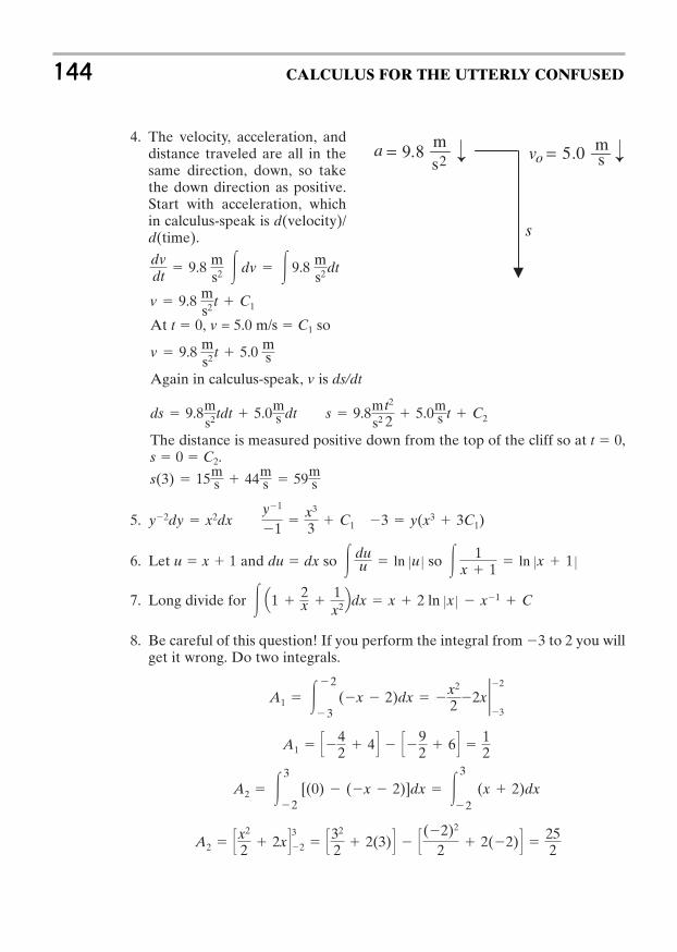
4. The velocity, acceleration, anddistance traveled are all in thesame direction, down, so takethe down direction as positive.Start with acceleration, whichin calculus-speak is d(velocity)/d(time).
At t 0, v = 5.0 m/s C1 so
Again in calculus-speak, v is ds/dt
The distance is measured positive down from the top of the cliff so at t 0,s 0 C2.
5.
6. Let u x 1 and du dx so so
7. Long divide for
8. Be careful of this question! If you perform the integral from 3 to 2 you willget it wrong. Do two integrals.
A2 Sx2
2 2xT3
2 S32
2 2(3)T S(2)2
2 2(2)T 252
A2 33
2[(0) (x 2)]dx 3
3
2(x 2)dx
A1 S42 4T S
92 6T
12
A1 32
3(x 2)dx
x2
2 2x 22
3
3 Q1 2x
1x2Rdx x 2 ln Zx Z x1 C
3 1x 1
ln Zx 1 Z3 duu ln Zu Z
y2dy x2dx y1
1
x3
3 C1 3 y(x3 3C1)
s(3) 15ms 44m
s 59ms
ds 9.8ms2tdt 5.0m
s dt s 9.8ms2
t2
2 5.0ms t C2
v 9.8 ms2 t 5.0 m
s
v 9.8 ms2 t C1
3 dv 3 9.8 ms2 dtdv
dt 9.8 m
s2
144 CALCULUS FOR THE UTTERLY CONFUSED
=sm
8.92
a = sm0.5ov
s
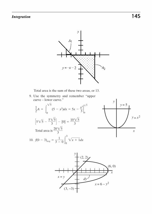
Total area is the sum of these two areas, or 13.
9. Use the symmetry and remember “uppercurve – lower curve.”
Total area is
10. f(0 3)avg 1
3 0 33
02x 1dx
20253
S525 525
3 T [0] 1025
3
12A 3
25
0(5 x2)dx 5x
x3
3225
0
Integration 145
y = x2
y = 5y
x
(6, 0)
x
y(2, 2)
(3, − 3)x = 6 − y2
x = ydy

Let .
11. This is a problem where graphing really helps. Look at the graph and real-ize that the integral has to be over dy. From the graph and a little algebrafind where the curves intersect.
AtAtRemember that the integral is from the most positive curve to the lesspositive curve.
A 32
3[(6 y2) y]dy 6y
y2
2 y3
32 23
1256
y 3, x 3y 2, x 2
y 6 y2 1 y2 y 6 (y 3)(y 2)
f(0 3)avg 13
23(x 1)3/2 2 3
0
169
29
149
u x 1 so du dx and the integral is 1u1/2du u3/2
3/2
146 CALCULUS FOR THE UTTERLY CONFUSED
xdxdy
xy
2
2
==
Cxy
xdxdy
+=
=
2
2⌠⌡
⌠⌡

CHAPTER 8
TRIGONOMETRICFUNCTIONS
You should read this chapter if you need to review or you need to learn about
Right angle trigonometry
Non-right angle triangles
Radians and small angles
Sine and cosine laws
Trigonometric functions
Differentiating trigonometric functions
Integrating trigonometric functions
147
Copyright © 2007 by The McGraw-Hill Companies, Inc. Click here for terms of use.
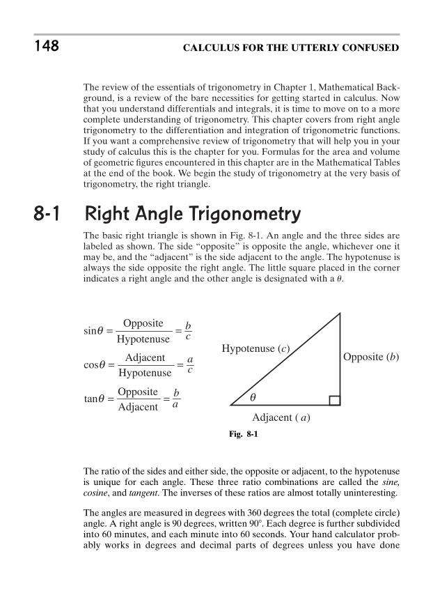
The review of the essentials of trigonometry in Chapter 1, Mathematical Back-ground, is a review of the bare necessities for getting started in calculus. Nowthat you understand differentials and integrals, it is time to move on to a morecomplete understanding of trigonometry. This chapter covers from right angletrigonometry to the differentiation and integration of trigonometric functions.If you want a comprehensive review of trigonometry that will help you in yourstudy of calculus this is the chapter for you. Formulas for the area and volumeof geometric figures encountered in this chapter are in the Mathematical Tablesat the end of the book. We begin the study of trigonometry at the very basis oftrigonometry, the right triangle.
8-1 Right Angle TrigonometryThe basic right triangle is shown in Fig. 8-1. An angle and the three sides arelabeled as shown. The side “opposite” is opposite the angle, whichever one itmay be, and the “adjacent” is the side adjacent to the angle. The hypotenuse isalways the side opposite the right angle. The little square placed in the cornerindicates a right angle and the other angle is designated with a .u
148 CALCULUS FOR THE UTTERLY CONFUSED
Fig. 8-1
The ratio of the sides and either side, the opposite or adjacent, to the hypotenuseis unique for each angle. These three ratio combinations are called the sine,cosine, and tangent. The inverses of these ratios are almost totally uninteresting.
The angles are measured in degrees with 360 degrees the total (complete circle)angle. A right angle is 90 degrees, written 90. Each degree is further subdividedinto 60 minutes, and each minute into 60 seconds. Your hand calculator prob-ably works in degrees and decimal parts of degrees unless you have done
Adjacent ( a)
Hypotenuse (c)Opposite (b)
ab
ca
cb
==
==
==
AdjacentOpposite
tanq
HypotenuseAdjacent
cosq
Hypotenuse
Oppositesinq
q
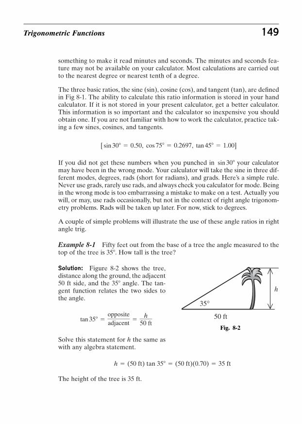
something to make it read minutes and seconds. The minutes and seconds fea-ture may not be available on your calculator. Most calculations are carried outto the nearest degree or nearest tenth of a degree.
The three basic ratios, the sine (sin), cosine (cos), and tangent (tan), are definedin Fig 8-1. The ability to calculate this ratio information is stored in your handcalculator. If it is not stored in your present calculator, get a better calculator.This information is so important and the calculator so inexpensive you shouldobtain one. If you are not familiar with how to work the calculator, practice tak-ing a few sines, cosines, and tangents.
, , ]
If you did not get these numbers when you punched in your calculatormay have been in the wrong mode. Your calculator will take the sine in three dif-ferent modes, degrees, rads (short for radians), and grads. Here’s a simple rule.Never use grads, rarely use rads, and always check you calculator for mode. Beingin the wrong mode is too embarrassing a mistake to make on a test. Actually youwill, or may, use rads occasionally, but not in the context of right angle trigonom-etry problems. Rads will be taken up later. For now, stick to degrees.
A couple of simple problems will illustrate the use of these angle ratios in rightangle trig.
Example 8-1 Fifty feet out from the base of a tree the angle measured to thetop of the tree is 35. How tall is the tree?
Solution: Figure 8-2 shows the tree,distance along the ground, the adjacent50 ft side, and the 35 angle. The tan-gent function relates the two sides tothe angle.
Solve this statement for h the same aswith any algebra statement.
The height of the tree is 35 ft.
h (50 ft) tan 35 (50 ft)(0.70) 35 ft
tan 35 oppositeadjacent
h
50 ft
sin 30
tan 45 1.00cos 75 0.2697[ sin 30 0.50
Trigonometric Functions 149
Fig. 8-2
35°
h
50 ft
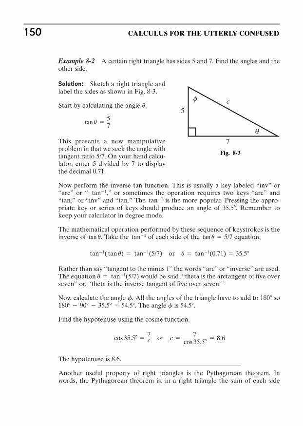
Example 8-2 A certain right triangle has sides 5 and 7. Find the angles and theother side.
Solution: Sketch a right triangle andlabel the sides as shown in Fig. 8-3.
Start by calculating the angle .
This presents a new manipulativeproblem in that we seek the angle withtangent ratio 5/7. On your hand calcu-lator, enter 5 divided by 7 to displaythe decimal 0.71.
Now perform the inverse tan function. This is usually a key labeled “inv” or“arc” or “ ,” or sometimes the operation requires two keys “arc” and“tan,” or “inv” and “tan.” The is the more popular. Pressing the appro-priate key or series of keys should produce an angle of 35.5. Remember tokeep your calculator in degree mode.
The mathematical operation performed by these sequence of keystrokes is theinverse of . Take the of each side of the equation.
or
Rather than say “tangent to the minus 1” the words “arc” or “inverse” are used.The equation would be said, “theta is the arctangent of five overseven” or, “theta is the inverse tangent of five over seven.”
Now calculate the angle . All the angles of the triangle have to add to so. The angle is .
Find the hypotenuse using the cosine function.
or
The hypotenuse is 8.6.
Another useful property of right triangles is the Pythagorean theorem. Inwords, the Pythagorean theorem is: in a right triangle the sum of each side
c 7
cos 35.5 8.6cos 35.5
7c
54.5f180 90 35.5 54.5180f
u tan1(5/7)
u tan1(0.71) 35.5tan1( tan u) tan1(5/7)
tan u 5/7tan1tan u
tan1tan1
tan u 57
u
150 CALCULUS FOR THE UTTERLY CONFUSED
Fig. 8-3
c5
7
q
f
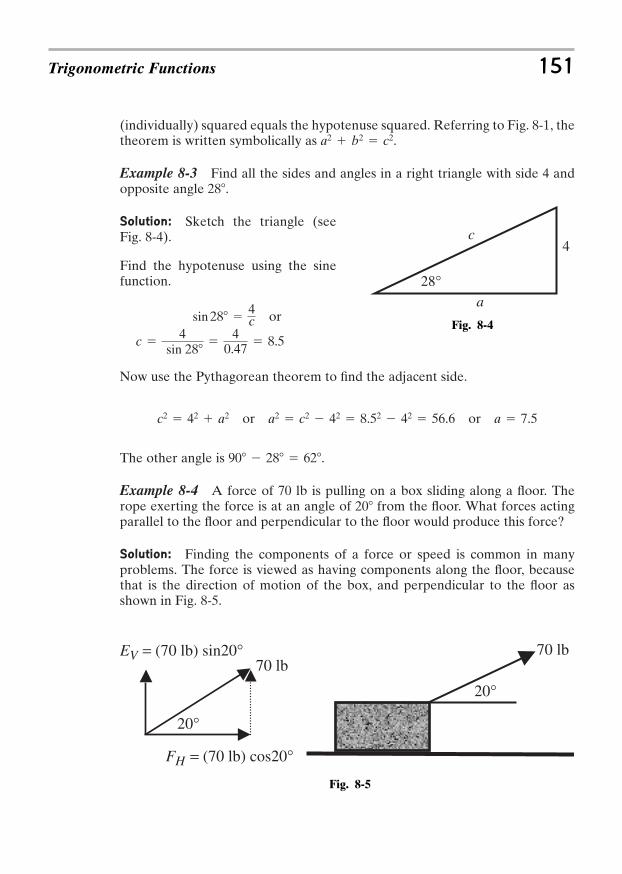
(individually) squared equals the hypotenuse squared. Referring to Fig. 8-1, thetheorem is written symbolically as .
Example 8-3 Find all the sides and angles in a right triangle with side 4 andopposite angle .
Solution: Sketch the triangle (seeFig. 8-4).
Find the hypotenuse using the sinefunction.
or
Now use the Pythagorean theorem to find the adjacent side.
or or
The other angle is .
Example 8-4 A force of 70 lb is pulling on a box sliding along a floor. Therope exerting the force is at an angle of 20 from the floor. What forces actingparallel to the floor and perpendicular to the floor would produce this force?
Solution: Finding the components of a force or speed is common in manyproblems. The force is viewed as having components along the floor, becausethat is the direction of motion of the box, and perpendicular to the floor asshown in Fig. 8-5.
90 28 62
a 7.5a2 c2 42 8.52 42 56.6c2 42 a2
c 4
sin 28
40.47 8.5
sin 28 4c
28
a2 b2 c2
Trigonometric Functions 151
Fig. 8-4
Fig. 8-5
28°a
4c
20°
70 lb 70 lb
20°
FH = (70 lb) cos20°
EV = (70 lb) sin20°
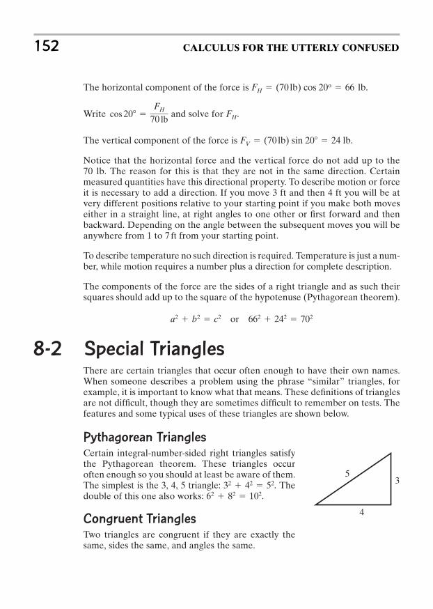
The horizontal component of the force is .
Write and solve for .
The vertical component of the force is .
Notice that the horizontal force and the vertical force do not add up to the70 lb. The reason for this is that they are not in the same direction. Certainmeasured quantities have this directional property. To describe motion or forceit is necessary to add a direction. If you move 3 ft and then 4 ft you will be atvery different positions relative to your starting point if you make both moveseither in a straight line, at right angles to one other or first forward and thenbackward. Depending on the angle between the subsequent moves you will beanywhere from 1 to from your starting point.
To describe temperature no such direction is required. Temperature is just a num-ber, while motion requires a number plus a direction for complete description.
The components of the force are the sides of a right triangle and as such theirsquares should add up to the square of the hypotenuse (Pythagorean theorem).
or
8-2 Special TrianglesThere are certain triangles that occur often enough to have their own names.When someone describes a problem using the phrase “similar” triangles, forexample, it is important to know what that means. These definitions of trianglesare not difficult, though they are sometimes difficult to remember on tests. Thefeatures and some typical uses of these triangles are shown below.
Pythagorean Triangles
Certain integral-number-sided right triangles satisfythe Pythagorean theorem. These triangles occuroften enough so you should at least be aware of them.The simplest is the 3, 4, 5 triangle: . Thedouble of this one also works: .
Congruent Triangles
Two triangles are congruent if they are exactly thesame, sides the same, and angles the same.
62 82 10232 42 52
662 242 702a2 b2 c2
7 ft
FV (70 lb) sin 20 24 lb
FHcos 20 FH
70 lb
FH (70 lb) cos 20o 66 lb
152 CALCULUS FOR THE UTTERLY CONFUSED
3
4
5
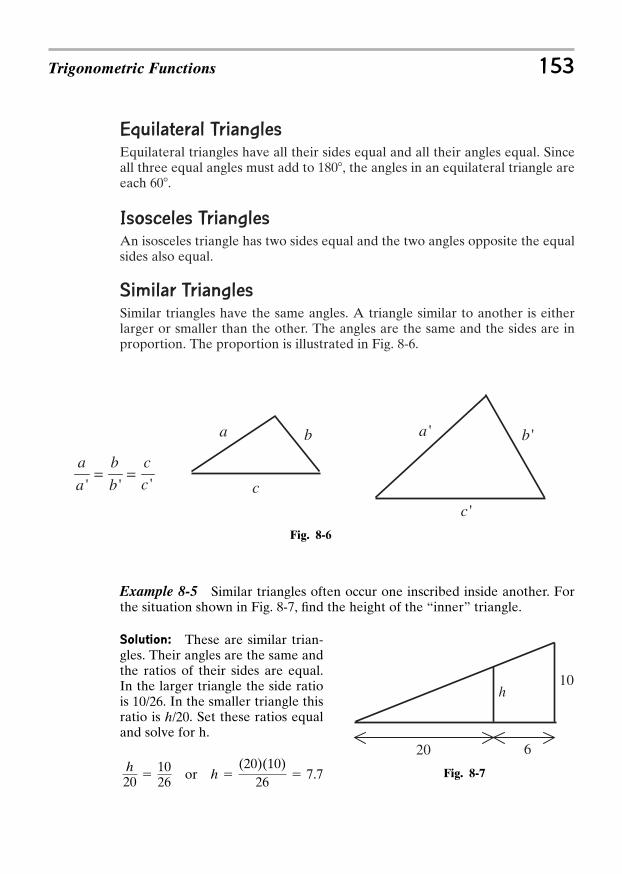
Equilateral Triangles
Equilateral triangles have all their sides equal and all their angles equal. Sinceall three equal angles must add to , the angles in an equilateral triangle areeach .
Isosceles Triangles
An isosceles triangle has two sides equal and the two angles opposite the equalsides also equal.
Similar Triangles
Similar triangles have the same angles. A triangle similar to another is eitherlarger or smaller than the other. The angles are the same and the sides are inproportion. The proportion is illustrated in Fig. 8-6.
60180
Trigonometric Functions 153
Fig. 8-6
Example 8-5 Similar triangles often occur one inscribed inside another. Forthe situation shown in Fig. 8-7, find the height of the “inner” triangle.
Solution: These are similar trian-gles. Their angles are the same andthe ratios of their sides are equal.In the larger triangle the side ratiois 10/26. In the smaller triangle thisratio is h/20. Set these ratios equaland solve for h.
or h (20)(10)
26 7.7h
20 1026
Fig. 8-7
'a 'b
'c
a b
c''' c
c
b
b
a
a==
10h
20 6
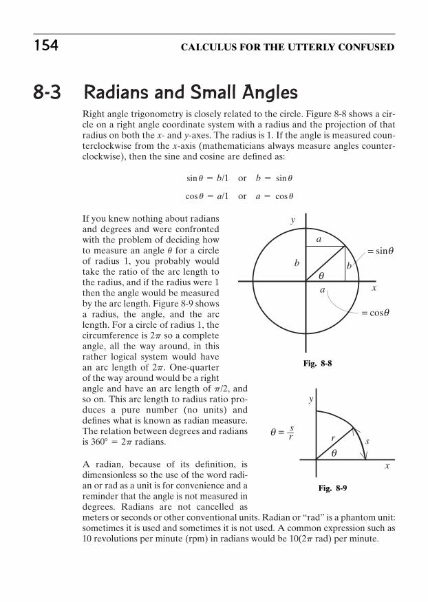
8-3 Radians and Small AnglesRight angle trigonometry is closely related to the circle. Figure 8-8 shows a cir-cle on a right angle coordinate system with a radius and the projection of thatradius on both the x- and y-axes. The radius is 1. If the angle is measured coun-terclockwise from the x-axis (mathematicians always measure angles counter-clockwise), then the sine and cosine are defined as:
or
or
If you knew nothing about radiansand degrees and were confrontedwith the problem of deciding howto measure an angle for a circleof radius 1, you probably wouldtake the ratio of the arc length tothe radius, and if the radius were 1then the angle would be measuredby the arc length. Figure 8-9 showsa radius, the angle, and the arclength. For a circle of radius 1, thecircumference is so a completeangle, all the way around, in thisrather logical system would havean arc length of . One-quarterof the way around would be a rightangle and have an arc length of , andso on. This arc length to radius ratio pro-duces a pure number (no units) anddefines what is known as radian measure.The relation between degrees and radiansis radians.
A radian, because of its definition, isdimensionless so the use of the word radi-an or rad as a unit is for convenience and areminder that the angle is not measured indegrees. Radians are not cancelled asmeters or seconds or other conventional units. Radian or “rad” is a phantom unit:sometimes it is used and sometimes it is not used. A common expression such as10 revolutions per minute (rpm) in radians would be 10( rad) per minute.2p
360 2p
p/2
2p
2p
u
a cos ucos u a/1
b sin usin u b/1
154 CALCULUS FOR THE UTTERLY CONFUSED
Fig. 8-8
x
y
bb
a
a
= cosq
= sinq
q
Fig. 8-9
r srs=
x
y
q
q
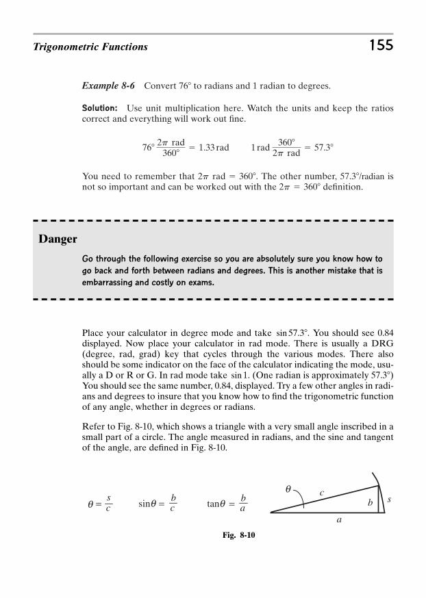
Example 8-6 Convert to radians and 1 radian to degrees.
Solution: Use unit multiplication here. Watch the units and keep the ratioscorrect and everything will work out fine.
You need to remember that . The other number, isnot so important and can be worked out with the definition.2p 360
57.3/radian2p rad 360
1 rad 3602p rad
57.3762p rad
360 1.33 rad
76
Trigonometric Functions 155
Danger
Go through the following exercise so you are absolutely sure you know how to
go back and forth between radians and degrees. This is another mistake that is
embarrassing and costly on exams.
Fig. 8-10
Place your calculator in degree mode and take . You should see 0.84displayed. Now place your calculator in rad mode. There is usually a DRG(degree, rad, grad) key that cycles through the various modes. There alsoshould be some indicator on the face of the calculator indicating the mode, usu-ally a D or R or G. In rad mode take . (One radian is approximately 57.3)You should see the same number, 0.84, displayed. Try a few other angles in radi-ans and degrees to insure that you know how to find the trigonometric functionof any angle, whether in degrees or radians.
Refer to Fig. 8-10, which shows a triangle with a very small angle inscribed in asmall part of a circle. The angle measured in radians, and the sine and tangentof the angle, are defined in Fig. 8-10.
sin 1
sin 57.3
sb
a
c
cs= c
b=sinq ab=tanqq
q
For small enough angles, s is approximately the same as b, and a is approxi-mately the same as c. Therefore, for small angles with the angle measured inradians, the angle, the sine of that angle, and the tangent of that angle are allnearly equal. The next problem illustrates the error in making the approxima-tion that the sine is the angle for some small angles.
Example 8-7 What is the difference (error) between the angle in radians, thesine, and the tangent for an angle of 0.1 radians?
Solution: As a warm up to this problem take the sine of and the tangentof .
The difference between these two is approximately 5 parts in 1000 or 0.5%error. Now
The difference between the sine and the angle at 0.1 radians is 2 parts in 1000.
The difference between the tangent and the angle at 0.1 radians is 3 parts in 1000.
The difference between the sine and the tangent at 0.1 radians is 5 parts in 1000.
Example 8-8 Redo Example 8-7 but at 0.5 radians, approximately .
Solution: , ,
The difference between and at 0.5 radians is about 4%, and the differ-ence between and is about 10%.
Use the approximation for angles up to and possibly ,but certainly not much bigger. If you find an old slide rule, you will see a scalefor sine and tangent that goes to 5.7
8-4 Non-Right Angle TrigonometryYou may encounter some situations requiring the side or angle in a non-righttriangle. The laws relating the sides and angles in non-right triangles are not
2010u sin u tan u
tan uu
sin uu
tan u 0.55sin u 0.48u 0.5
30
tan (0.1) 0.1003
sin (0.1) 0.0998
u (in radians) 0.1000
tan 5.7 0.0998sin 5.7 0.0993
5.75.7
156 CALCULUS FOR THE UTTERLY CONFUSED
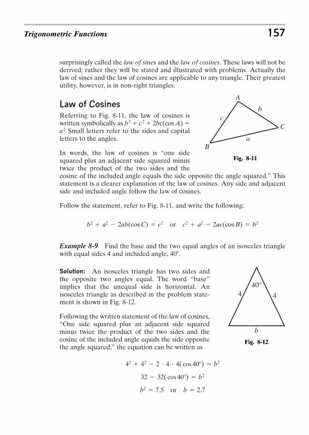
surprisingly called the law of sines and the law of cosines. These laws will not bederived; rather they will be stated and illustrated with problems. Actually thelaw of sines and the law of cosines are applicable to any triangle. Their greatestutility, however, is in non-right triangles.
Law of Cosines
Referring to Fig. 8-11, the law of cosines iswritten symbolically as b2 c2 2bc(cos A) a2 Small letters refer to the sides and capitalletters to the angles.
In words, the law of cosines is “one sidesquared plus an adjacent side squared minustwice the product of the two sides and thecosine of the included angle equals the side opposite the angle squared.” Thisstatement is a clearer explanation of the law of cosines. Any side and adjacentside and included angle follow the law of cosines.
Follow the statement, refer to Fig. 8-11, and write the following:
or
Example 8-9 Find the base and the two equal angles of an isosceles trianglewith equal sides 4 and included angle, .
Solution: An isosceles triangle has two sides andthe opposite two angles equal. The word “base”implies that the unequal side is horizontal. Anisosceles triangle as described in the problem state-ment is shown in Fig. 8-12.
Following the written statement of the law of cosines,“One side squared plus an adjacent side squaredminus twice the product of the two sides and thecosine of the included angle equals the side oppositethe angle squared,” the equation can be written as
or b 2.7b2 7.5
32 32( cos 40) b2
42 42 2 4 4( cos 40) b2
40
c2 a2 2ac(cos B) b2b2 a2 2ab(cos C) c2
Trigonometric Functions 157
Fig. 8-12
40°44
b
Fig. 8-11
a
bc
A
B
C
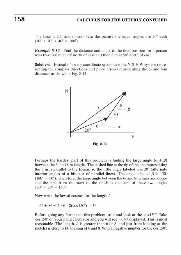
The base is 2.7, and to complete the picture the equal angles are each.
Example 8-10 Find the distance and angle to the final position for a personwho travels 6 m at north of east and then 8 m at north of east.
Solution: Instead of an x-y coordinate system use the N-S-E-W system repre-senting the compass directions and place arrows representing the 6- and 8-mdistances as shown in Fig. 8-13.
5020
(70 70 40 180)70
158 CALCULUS FOR THE UTTERLY CONFUSED
Fig. 8-13
50°
20°
N
E
6
8l
a
b
Perhaps the hardest part of this problem is finding the large angle between the 6- and 8-m lengths. The dashed line at the tip of the line representingthe 6 m is parallel to the E-axis, so the little angle labeled is (alternateinterior angles of a bisector of parallel lines). The angle labeled is ( . Therefore, the large angle between the 6- and 8-m lines and oppo-site the line from the start to the finish is the sum of these two angles
.
Now write the law of cosines for the length l.
Before going any farther on this problem, stop and look at the . Takeon your hand calculator and you will see 0.87 displayed. This is most
reasonable. The length, l, is greater than 6 or 8, and just from looking at thesketch l is close to 14, the sum of 6 and 8. With a negative number for the ,cos 150
cos 150cos 150
62 82 2 6 8(cos 150) l 2
130 20 150
180 50)130b
20a
(a b)
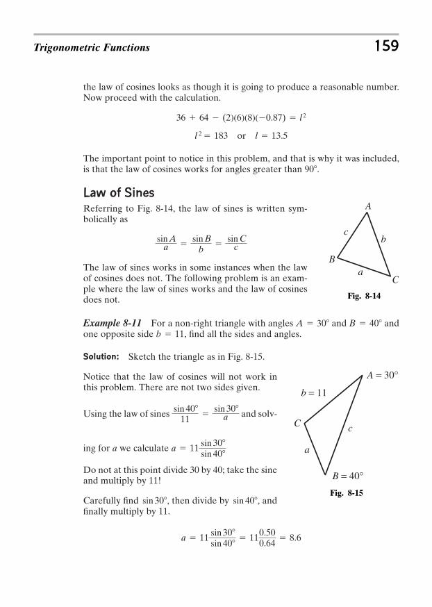
the law of cosines looks as though it is going to produce a reasonable number.Now proceed with the calculation.
or
The important point to notice in this problem, and that is why it was included,is that the law of cosines works for angles greater than .
Law of Sines
Referring to Fig. 8-14, the law of sines is written sym-bolically as
The law of sines works in some instances when the lawof cosines does not. The following problem is an exam-ple where the law of sines works and the law of cosinesdoes not.
Example 8-11 For a non-right triangle with angles and andone opposite side , find all the sides and angles.
Solution: Sketch the triangle as in Fig. 8-15.
Notice that the law of cosines will not work inthis problem. There are not two sides given.
Using the law of sines and solv-
ing for a we calculate
Do not at this point divide 30 by 40; take the sineand multiply by 11!
Carefully find , then divide by , andfinally multiply by 11.
a 11 sin 30sin 40
110.500.64
8.6
sin 40sin 30
a 11 sin 30sin 40
sin 4011
sin 30
a
b 11B 40A 30
sin Aa
sin Bb
sin C
c
90
l 13.5l 2 183
36 64 (2)(6)(8)(0.87) l 2
Trigonometric Functions 159
Fig. 8-15
B = 40°
b = 11
A = 30°
C c
a
Fig. 8-14
a
A
b
B
c
C

The angle C is .
And finally use the law of sines to find side c.
or
Example 8-12 You need to determine the distances from two points, A andB, on one side of a canyon to a single point, C, on the opposite side of thecanyon. At point A you measure an angle of between points B and C. Atpoint B, 300 m from point A, you measure an angle of between points A andC. What is the distance from A to C and B to C?
Solution: Draw a diagram and use thelaw of sines. The angle at C is from 180 65 40 75. Set up the law of sines andnote that this law can be written upsidedown from the normal way (see Fig. 8-16).
8-5 Trigonometric FunctionsThe definition of the trigonometric functions starts with the right triangleinscribed in the unit circle first shown in Fig. 8-8.
Place a unit circle on a right angle coordinate system as shown in Fig. 8-17. Thesides of the inscribed triangle are the sine and cosine of the angle, . These sidesof the inscribed triangle are also the projections of the point on the circle thatdefines the angle on the axes. The projection on the x-axis is the cosine of , andthe projection on the y-axis is the sine of .
As the point defining the angle moves around the circle in a counterclockwisemanner, the projection on the x-axis traces out the cosine function and the
u
u
u
b sin 40sin 75
300 200
a sin 65sin 75
300 281
300sin 75
a
sin 65
bsin 40
4065
c 11 sin 110sin 40
110.940.64
16.2sin 110c
sin 4011
(180 30 40 110)110
160 CALCULUS FOR THE UTTERLY CONFUSED
Fig. 8-16
14
A B
C
ab
c65° 40°
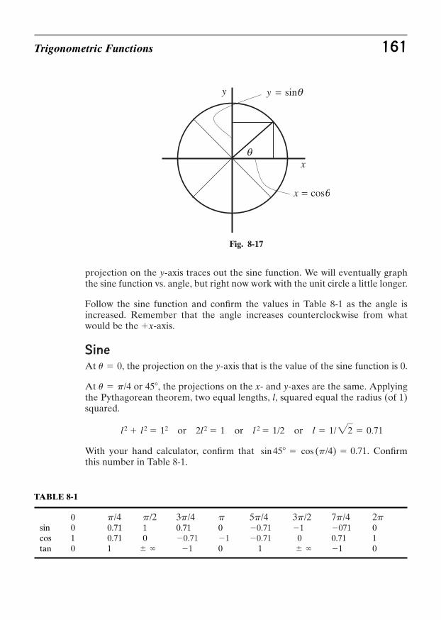
projection on the y-axis traces out the sine function. We will eventually graphthe sine function vs. angle, but right now work with the unit circle a little longer.
Follow the sine function and confirm the values in Table 8-1 as the angle isincreased. Remember that the angle increases counterclockwise from whatwould be the x-axis.
Sine
At , the projection on the y-axis that is the value of the sine function is 0.
At or , the projections on the x- and y-axes are the same. Applyingthe Pythagorean theorem, two equal lengths, l, squared equal the radius (of 1)squared.
or or or
With your hand calculator, confirm that . Confirmthis number in Table 8-1.
sin 45 cos (p/4) 0.71
l 1/22 0.71l 2 1/22l 2 1l 2 l 2 12
45u p/4
u 0
Trigonometric Functions 161
TABLE 8-1
0sin 0 0.71 1 0.71 0 0cos 1 0.71 0 0 0.71 1tan 0 1 0 1 1 0 `1 `
0.7110.7107110.71
2p7p/43p/25p/4p3p/4p/2p/4
Fig. 8-17
x
cosq=x
sinqyy
q
=
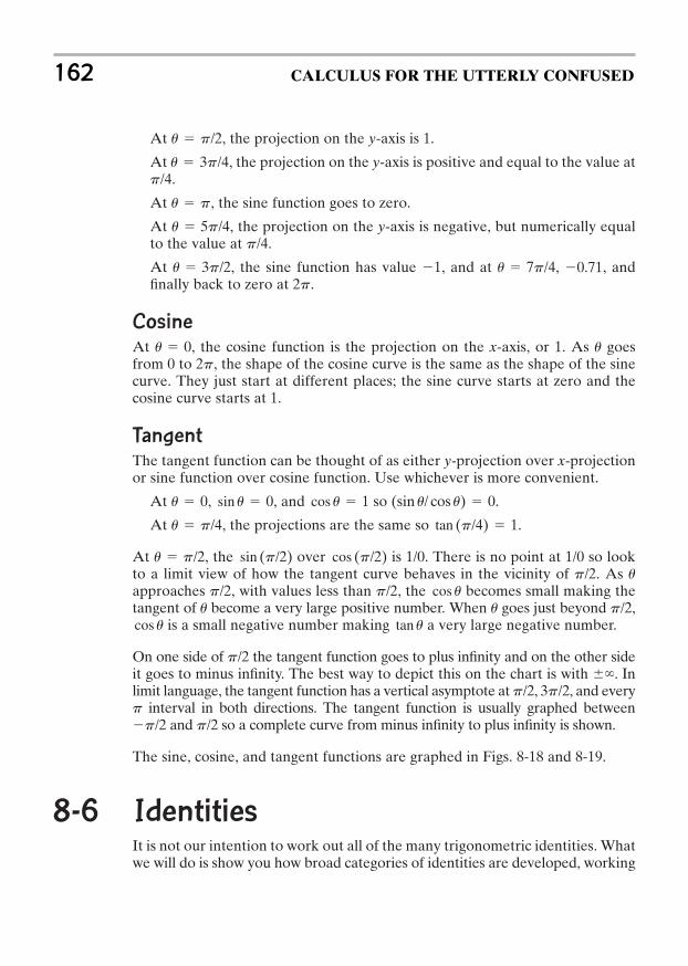
At , the projection on the y-axis is 1.
At , the projection on the y-axis is positive and equal to the value at.
At , the sine function goes to zero.
At , the projection on the y-axis is negative, but numerically equalto the value at .
At , the sine function has value 1, and at , 0.71, andfinally back to zero at .
Cosine
At the cosine function is the projection on the x-axis, or 1. As goesfrom 0 to the shape of the cosine curve is the same as the shape of the sinecurve. They just start at different places; the sine curve starts at zero and thecosine curve starts at 1.
Tangent
The tangent function can be thought of as either y-projection over x-projectionor sine function over cosine function. Use whichever is more convenient.
At , , and so .
At , the projections are the same so .
At , the over is . There is no point at so lookto a limit view of how the tangent curve behaves in the vicinity of . As approaches , with values less than , the becomes small making thetangent of become a very large positive number. When goes just beyond ,
is a small negative number making a very large negative number.
On one side of the tangent function goes to plus infinity and on the other sideit goes to minus infinity. The best way to depict this on the chart is with . Inlimit language, the tangent function has a vertical asymptote at , , and every
interval in both directions. The tangent function is usually graphed betweenand so a complete curve from minus infinity to plus infinity is shown.
The sine, cosine, and tangent functions are graphed in Figs. 8-18 and 8-19.
8-6 IdentitiesIt is not our intention to work out all of the many trigonometric identities. Whatwe will do is show you how broad categories of identities are developed, working
p/2p/2p
3p/2p/2
p/2
tan ucos up/2uu
cos up/2p/2up/2
1/01/0cos (p/2)sin (p/2)u p/2
tan (p/4) 1u p/4
(sin u/ cos u) 0cos u 1sin u 0u 0
2p,uu 0,
2pu 7p/4u 3p/2
p/4u 5p/4
u p
p/4u 3p/4
u p/2
162 CALCULUS FOR THE UTTERLY CONFUSED
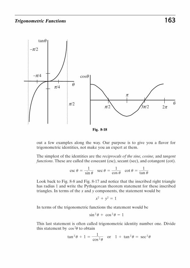
out a few examples along the way. Our purpose is to give you a flavor fortrigonometric identities, not make you an expert at them.
The simplest of the identities are the reciprocals of the sine, cosine, and tangentfunctions. These are called the cosecant (csc), secant (sec), and cotangent (cot).
Look back to Fig. 8-8 and Fig. 8-17 and notice that the inscribed right trianglehas radius 1 and write the Pythagorean theorem statement for these inscribedtriangles. In terms of the x and y components, the statement would be
In terms of the trigonometric functions the statement would be
This last statement is often called trigonometric identity number one. Dividethis statement by to obtain
or 1 tan 2 u sec 2 u tan 2 u 1 1
cos 2 u
cos 2u
sin 2 u cos 2 u 1
x2 y2 1
csc u 1
sin u sec u
1cos u cot u
1tan u
Trigonometric Functions 163
Fig. 8-18
tanq
cosq
q
q
-p/2
p/22pp/2 3p/2
-p/4
p/4
p
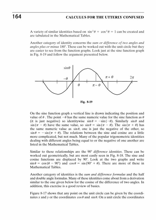
A variety of similar identities based on can be created andare tabulated in the Mathematical Tables.
Another category of identity concerns the sum or difference of two angles andangles plus or minus . These can be worked out with the unit circle but theyare easier to see from the function graphs. Look just at the sine function graphin Fig. 8-19 and follow the argument presented below.
180
sin 2 u cos 2 u 1
164 CALCULUS FOR THE UTTERLY CONFUSED
On the sine function graph a vertical line is drawn indicating the position andvalue of . The point has the same numeric value for the sine function as (it is just negative) so identitywise . Similarly and
have the same value, so . The hasthe same numeric value as , one is just the negative of the other, so
. The relations between the sine and cosine are a littlemore complicated, but not much. Many of the popular trigonometric identitiesdealing with different angles being equal to or the negative of one another arelisted in the Mathematical Tables.
Similar to these relationships are the difference identities. These can beworked out geometrically, but are most easily seen in Fig. 8-18. The sine andcosine functions are displaced by . Look at the two graphs and write
and . There are more of these inMathematical Tables.
Another category of identities is the sum and difference formulas and the halfand double angle formulas. Many of these identities come about from a derivationsimilar to the one given below for the cosine of the difference of two angles. Inaddition, this exercise is a good review of basics.
Figure 8-17 shows that any point on the unit circle can be given by the coordi-nates x and y or the coordinates and . On a unit circle the coordinatessin ucos u
cos u sin (90 u)sin u cos (u 90)90
90
sin u sin (p u)sin u
sin (p u)sin u sin (p u)sin (p u)sin usin u sin (u)
uuu
Fig. 8-19
2p
sinq
−q
q p − q
p + q
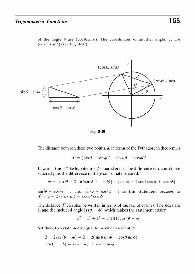
of the angle are . The coordinates of another angle, , are(see Fig. 8-20).(cosf, sinf)
f(cos u, sin u)u
Trigonometric Functions 165
Fig. 8-20
x
y
d(cosf, sinf)
(cosq, sinq)
cosq - cosf
sinq - sinf fq
The distance between these two points, d, in terms of the Pythagorean theorem, is
In words, this is “the hypotenuse d squared equals the difference in x-coordinatesquared plus the difference in the y-coordinate squared.”
and so this statement reduces to
The distance can also be written in terms of the law of cosines. The sides are1, and the included angle is , which makes the statement easier.
Set these two statements equal to produce an identity.
cos (u f) sin u sinf cos u cosf
2 2 cos (u f) 2 2( sin u sinf cos u sinf)
d 2 12 12 2(1)(1) cos (u f)
(u f)d 2
d 2 2 2 sin u sinf 2 cos u cosfsin 2f cos 2f 1sin 2u cos 2u 1
d 2 [sin 2u 2 sin u sinf sin 2f] [cos 2u 2 cos u cosf cos 2f]
d 2 ( sin u sinf)2 ( cos u cosf)2
This identity gives the cosine of the difference of two angles in terms of the sinesand cosines of the individual angles. A myriad of sum and difference of twoangle formulas as well as double and half angle formulas come from exercisessimilar to this one. Fortunately they are all tabulated in many places, mostnotable in Mathematical Tables in the back of this book. These tables given hereare not complete, just sufficient for most of the problems you will encounter.
8-7 Differentiating Trigonometric
FunctionsA somewhat intuitive justification for the derivative of the sine function was givenin Chapter 3, Derivatives. Now it is time to look a little more closely at deriva-tives of trigonometric functions and apply those derivatives to some problems.
The derivative of the sine function is the cosine function and the derivative ofthe cosine function is the negative of the sine function. The justification for thederivative of the sine function (Chapter 3) is enough to give you a feel for howthe derivatives of trigonometric functions come about. The more popular deriv-atives are listed below, with a larger list presented in the Mathematical Tables.
, ,
One thing that occurs fairly often in trigonometric functions is that the variable,the , the x, or whatever is not simply or x but something more complicated,like 2x, for example.
Example 8-13 Find the derivative of .
Solution: This kind of problem is best done in an implicit style. Write and then differentiate according to the formula for the differential of the cosine.
In words, “the differential of is equal to minus (times the) differ-ential of 2x.” And the differential of 2x is 2dx.
With this experience .
The implicit derivative approach with the equation written in one line is theeasier method.
ddx
( cos 2x) 2 sin 2x
sin 2xcos 2x
d(cos 2x) (sin 2x)d(2x) 2(sin 2x)dx
d(cos 2x)
cos 2x
uu
d(tan u) sec 2udud(cos u) sin udud(sin u) cos udu
166 CALCULUS FOR THE UTTERLY CONFUSED
Example 8-14 Find for .
Solution: Before differentiating the we first have to deal with the cube of. If the problem were , the implicit style derivative would read
.
For the function , an approach parallel to the one above would pro-duce .
The is , so .
Example 8-15 Find of .
Solution: Go slowly and don’t get confused. Do the tangent squared part ofthe derivative and then take care of the part.
or
The problem can be rewritten using the identity .Rewrite the problem as
Take the differential in implicit form
so
Example 8-16 What is the angle between and the x-axis when thecurve crosses the axis?
Solution: This is one of those innocent looking problems that look easy butperhaps is not so easy. Oh, but it is not difficult for Captain Calculus, because“The Captain” always “thinks calculus.”
y cos 3x
dydu
4 tan 2u sec 22u
dy 2 sec 2ud sec 2u 2 sec 2u( tan 2u sec 2ud2u) 4 tan 2u sec 22udu
y sec 22u 1
sec 2 2u 1 tan2 2u
dydu
4(tan 2u)(sec 2 2u)d 4(tan 2u)(sec 2 2u)du
dy 2(tan 2u)(sec 2 2u)d(2u)
dy 2(tan 2u)d(tan 2u)
2u
y tan 22udydx
dydx
3( sin 2x)( cos x)( cos x)dxd( sin x)
dy 3( sin 2x)d( sin x)y sin 3x
dy 3u2duy u3sin x
sin x
y sin 3xdydx
Trigonometric Functions 167
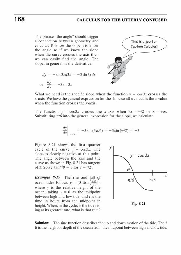
The phrase “the angle” should triggera connection between geometry andcalculus. To know the slope is to knowthe angle so if we know the slopewhen the curve crosses the axis thenwe can easily find the angle. Theslope, in general, is the derivative.
or
What we need is the specific slope when the function crosses thex-axis. We have the general expression for the slope so all we need is the x-valuewhen the function crosses the x-axis.
The function crosses the x-axis when or .Substituting into the general expression for the slope, we calculate
Figure 8-21 shows the first quartercycle of the curve . Theslope is clearly negative at this point.The angle between the axis and thecurve as shown in Fig. 8-21 has tangentof 3. Solve for .
Example 8-17 The rise and fall ofocean tides follows ,where y is the relative height of theocean, taking as the midpointbetween high and low tide, and t is thetime in hours from the midpoint inheight. When, in the cycle, is the tide ris-ing at its greatest rate, what is that rate?
Solution: The sine function describes the up and down motion of the tide. The 3ft is the height or depth of the ocean from the midpoint between high and low tide.
y 0
y (3 ft)sinQ2p11
tR
u 72tan1u 3
y cos 3x
dydx2xp/6
3 sin (3p/6) 3 sin (p/2) 3
p/6x p/63x p/2y cos 3x
y cos 3x
dydx
3 sin 3x
dy sin 3xd3x 3 sin 3xdx
168 CALCULUS FOR THE UTTERLY CONFUSED
This is a job for
Captain Calculus!
C
Fig. 8-21
x
y
y 3xcos=
p /6 p /3
q
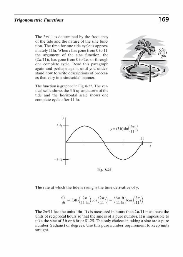
The is determined by the frequencyof the tide and the nature of the sine func-tion. The time for one tide cycle is approx-imately 11hr. When t has gone from 0 to 11,the argument of the sine function, the
, has gone from 0 to , or throughone complete cycle. Read this paragraphagain and perhaps again, until you under-stand how to write descriptions of process-es that vary in a sinusoidal manner.
The function is graphed in Fig. 8-22. The ver-tical scale shows the 3 ft up and down of thetide and the horizontal scale shows onecomplete cycle after 11 hr.
2p(2p/11)t
2p/11
Trigonometric Functions 169
Fig. 8-22
11
t
y
−3 ft
3 ft= ty
112πft)sin3(
The rate at which the tide is rising is the time derivative of y.
The has the units . If t is measured in hours then must have theunits of reciprocal hours so that the sine is of a pure number. It is impossible totake the sine of or 6 hr or $1.25. The only choices in taking a sine are a purenumber (radians) or degrees. Use this pure number requirement to keep unitsstraight.
3 ft
2p/111/hr2p/11
dydt
(3ft)Q2p
11 hrR cos Q
2p11
tR Q6p11
fthrR cos Q
2p11
tR
The rate at which the tide is rising, , is a maximum when is max-imum. The cosine function is a maximum at 0 or in this case at . This point,
, corresponds to the midpoint between high and low tide (see Fig. 8-21).
The tide is rising at its fastest rate midway between high and low tide.
The maximum rate is .
Second Solution: Captain Calculus, who always “thinks calculus,” would notneed to take a derivative to know when the tide was rising at maximum rate.The Captain would look at the sine curve (Fig. 8-22) describing how the oceanlevel was going up and down with the tide and ask where the slope had thegreatest positive value. Just by looking at the curve, the maximum positiveslope and the greatest rate of rise of the tide are at the midpoint between highand low tide.
8-8 Integrating Trigonometric FunctionsThree basic integral formulas can be obtained by taking the antiderivative ofthe differential formulas at the beginning of the previous section.
, ,
, ,
Two other popular integrals of trigonometric functions are
,
These and a few other trigonometric integrals are listed at the back of the bookin the Mathematical Tables.
Handling integrals other than the standard integral, , is alittle harder with integrals than it was with differentials. The following problemillustrates the procedure.
1 sin , cos , or tan (x)dx
3 cot udu ln (sin u)3 tan udu ln (cos u)
3 sec 2udu tan u3 sin udu cos u3 cos udu sin u
3 d(tan u) 3 sec 2 udu3 d(cos u) 3 sin udu3 d(sin u) 3 cos udu
2p11
fthr
0.57 fthr
t 0t 0
cos (2p/11)tdy/dt
170 CALCULUS FOR THE UTTERLY CONFUSED

Example 8-18 Find the integral of .
Solution: Here again is a case where is known but this is not the
exact problem. The first step in this problem is to make the look like.
Constants can be placed inside or outside the integral sign; it makes no differ-ence. To make this problem read , multiply by and take the 2 in thenumerator inside the integral and associate it with the d , and leave the remain-ing outside the integral.
Now the integral is in the form and has the following solution:
Example 8-19 Find .
Solution: Don’t be fooled by this integral. It is not a power law problem. It isnot an easy integral and do not get involved in trying to work it out. Go to theMathematical Tables or some table of integrals and copy the answer.
Example 9-20 Find the average value of the sine function from 0 to .
Solution: The average value of the function uses the definition of the averagevalue of a function over a range (see Chapter 7, Integration). The integration isover the first half-cycle of the sine function as shown in Fig. 8-22. The averagevalue of the function from 0 to is
x Zavg 1
p 0 3p
0sin udu
px sin u
p
y 3 sin 3 udu 13 cosu(sin 2u 2)
y 1 sin 3udu
y 12(cos 2u)
12 cos 2u
1 sin udu
y 12 3 sin 2ud2u
1/2u
2/21 sin udu
1 sin udu1 sin 2udu
1 sin udu
y 3 sin 2udu
Trigonometric Functions 171
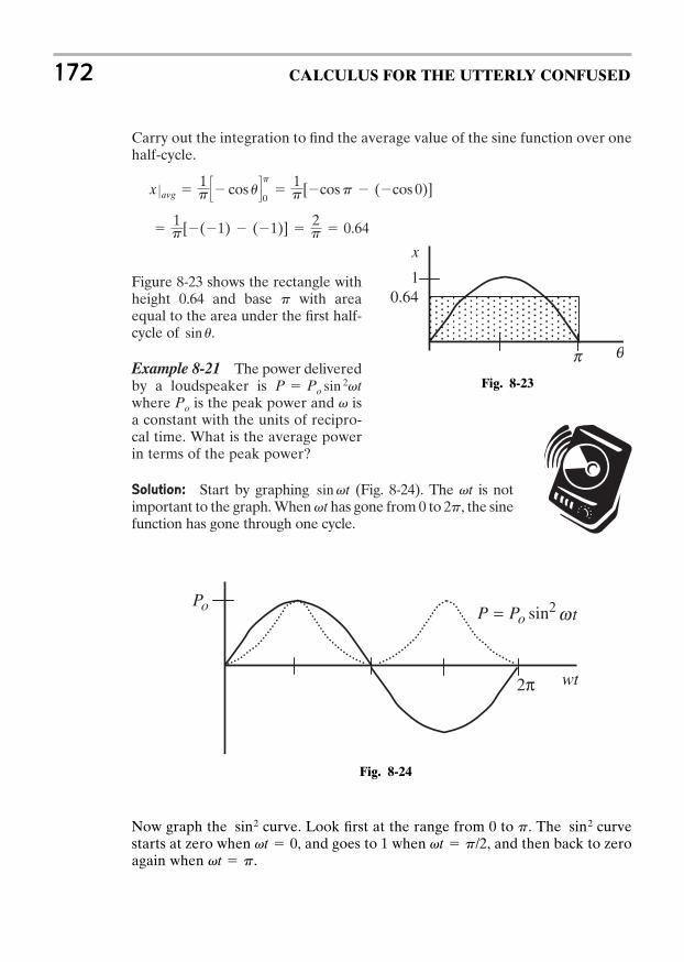
Carry out the integration to find the average value of the sine function over onehalf-cycle.
Figure 8-23 shows the rectangle withheight 0.64 and base with areaequal to the area under the first half-cycle of .
Example 8-21 The power deliveredby a loudspeaker is where is the peak power and isa constant with the units of recipro-cal time. What is the average powerin terms of the peak power?
Solution: Start by graphing (Fig. 8-24). The is notimportant to the graph. When has gone from 0 to 2 , the sinefunction has gone through one cycle.
pvtvtsinvt
vPo
P Po sin 2vt
sin u
p
1p[(1) (1)]
2p 0.64
x Zavg 1p S cos uT
p
0
1p[cosp (cos 0)]
172 CALCULUS FOR THE UTTERLY CONFUSED
Fig. 8-23
x
10.64
p q
Fig. 8-24
PP o2sin=
2π tw
oPw t
Now graph the curve. Look first at the range from 0 to . The curvestarts at zero when , and goes to 1 when , and then back to zeroagain when .vt p
vt p/2vt 0 sin2p sin2

The curve, however, has a different shape from the sin curve. The uniqueshape of the curve is due to the fact that when a number less than 1 issquared, the result is smaller [ ]. The smaller the number, the smallerthe result on squaring [ but ].
When the sin curve is negative, the curve is positive (see Fig. 8-24). Thecurve is periodic in so the average value of the curve is the average
value between 0 and .
The average value of this -type function follows the definition of the aver-age value of the function.
The integral is (from the Mathematical Tables) so
The average power for the loudspeaker is one-half the peak power.
Example 8-22 What is the area bounded by , , and ?
Solution: The sine and cosine functions areshown in Fig. 8-25. The integral of the areabetween the curves is in the x-direction andhas form . The integral isfrom to the intersection point of thetwo curves. At this point
or or
From the graph of , when. Check the number in your hand cal-
culator. Take the inverse tangent of 1. Table 8-1also shows equal to at sothe complete integral, complete with limits, is
A 3p/4
0( cos x sin x)dx
x p/4cos xsin x
x p/4tan x 1tan x
tan x 1sin xcos x 1sin x cos x
x 01( cos x sin x)dx
x 0y2 sin xy1 cos x
Pavg Pop B1
2vt 14 sin 2vtR
Pop b Bp2
14 sin 2pR B0
14 sin 0R r
Po
2
12 u
14 sin 2u1 sin 2 udu
P Zavg 1
p 0Po 3p
0sin 2vtd(vt)
sin 2
p
sin 2psin 2sin 2
0.32 0.090.92 0.810.52 0.25
sin2 sin2
Trigonometric Functions 173
Fig. 8-25
y
x
y sin x2 =
y cos x1=
Example 8-23 A certain company is selling golf shirts with the college logothrough college bookstores. Because of an expanding market overall sales aregrowing at 2t thousands of dollars per month, t. Superimposed over this lineargrowth is a sinusoidal variation following the academic year and described by
in thousands of dollars and with corresponding to January.Determine the rate of sales at the end of March .
Solution: The equation describing sales is
The general expression for the change in sales is
The rate of change of sales at the end of March is obtained by evaluat-
ing the at .
At the end of March sales are at the linear rate of 2 thousand dollars per month.
Example 8-24 For the previous problem find the total sales for the 3 monthsfrom January through March.
Solution: Sales follow . The total sales over any periodis the integral of S, with appropriate limits. The limits for this January to Marchperiod are t 0 and t 3.
S 2t 0.1 cos 2p t12
dSdt2t3
2 (0.1)p
6sinp2 2
t 3dSdt
(t 3)
dS 2dt (0.1) sin 2p t12
dQ2p t12R or dS
dt 2
(0.1)p6
sin 2p t12
S 2t 0.1 cos 2p t12
(t 3)t 0(0.1) cos 2p t
12
A 0.71 0.71 1 1.41 1 0.41
A [ sin x cos x]p/40 S sinp4 cosp4 T [ sin 0 cos 0]
174 CALCULUS FOR THE UTTERLY CONFUSED
Total sales for the January to March period were 9.2 thousands of dollars.
Solve right and non-right triangles
Know how to derive simple identities
Differentiate trigonometric functions
Integrate trigonometric functions
Apply differentiation and integration to practical problems
Use tables for differentiation of trigonometric functions
Use tables for integration of trigonometric functions
PROBLEMS
1. A cross country skier skis 1.2 km north and then 2.0 km east. How far andin what direction is she from her starting point?
2. Two sides of a non-right triangle are 4.0 and 5.0 and the included angle is38. What are the other angles and side?
3. Convert: 2 rad to degrees, to degrees and 85 to radians.4. Find the derivative of .5. Find the derivative of .6. .
7. Evaluate .
8. Evaluate .1x sin x2dx1 sec x( sec x tan x)dx
y(x) tan (x2) sec (2 3x)f(t) cos 2tf(s) sin (3s 1)p/3
S0S3 9 0.6p 9.2
S0S3 9 0.6p S sin
p2 sin 0T
S0S3 t2 2 30
0.6p sinpt
62 30
S0S3 33
02tdt 3
3
00.1 6p cospt
6dpt
6
S0S3 33
0[2t (0.1) cospt/6]dt
Trigonometric Functions 175

176 CALCULUS FOR THE UTTERLY CONFUSED
9. Sales of a certain product follow a cyclical sales pattern according to, where t is the time in months measured from
January 1 and S is the number of sales in thousands. What is the averagesales for the first quarter of the year?
10. What is the area under the curve of x sinx from 0 to 2 .
ANSWERS
You may need to consult a table of differen-tials and integrals to solve these problems.1. Draw a vector diagram representing her
trip. Her distance from the starting pointis
The angle is
2. Use the law of cosines to find side b.
so b 3.08Use the law of sines to find A and C.
3.
4. Use the chain rule and think of (3s + 1) as another variable, u.
5.6.
7.
8. Make a change of variable: let . If there were no x out-side the argument of the sin then this would be a much more difficult integral.12 3 sin udu
12 cos u so integral is
12 cos x2
u x2 so du 2xdxtan x sec x C1 sec 2xdx 1 sec x tan xdx
dydx
2x sec 2(x2) 3 sec (2 3x) tan (2 3x)
dy sec 2(x2)d(x2) sec (2 3x) tan (2 3x)d(2 3x)f r(t) 2 sin t cos t
df cos (3s 1)d(3s 1) 3 cos (3s 1)ds 1 f r(s) 3 cos (3s 1)
2 rad 360o
2p rad 115 p3
3602p 60 85
2p360
1.48
sin C 4
3.08 sin 38 C 53
sin A 5
3.08 sin 38 A 88
sin A5.0
sin 383.08
sin C4.0
b2 42 52 2(4)(5) cos 38
u tan1 21.2
59
R 21.22 2.0 2 2.3 km
p
S(t) 30 12 cospt8
1.2
2.0
Rq
a = 5.0
bc = 4.0
A
B = 38°
C
9. This is an average value integral over the first 3 months of the year.
The average monthly sales for the first 3 months is 39 thousand.10. The curve is a somewhat distorted sin function. The area is the definite inte-
gral of the function over the interval.
. This integral can be performed by a technique called inte-
gration by parts which is taken up in the next chapter or it can be “guessed”with just a few tries. Follow along on the guessing approach. First a cosineis involved because of the integral of the sine, so start with cosx and differ-entiate to find the integrand. The differential of cos x is sin x which is astart. Now for a little better guess try x cos x which has differential xsinxwhich is the integrand but it has the added differential term cos x. This istaken care of by adding a sinx. The final integrand is from d(x cos x sin x) x sin x cos x cos x x sinx. A little tortured, but not impossible.With a little experience these can go rather quickly. This, however, is prob-ably not high on your list of skills to learn. Buy mathematical tables.
A 1p0 x sin xdx
Avg Sales 13 S30t
96p sinpt
8 T3
0
13 S90
96p sin 3p
8 T 39
Avg Sales 13 S30 3
3
0dt 12 8
p 33
0cospt
8 dpt8 T
Avg Sales 1
3 0 33
0Q30 12 cospt
8 Rdt 13 S30 3
3
0dt 12 3
3
0cospt
8 dtT
Trigonometric Functions 177

This page intentionally left blank
CHAPTER 9
EXPONENTSAND LOGARITHMS
You should read this chapter if you need to review or you need to learn about
Basics of exponents and logarithms
Exponential functions
The number e
Growth and decay problems
Limited growth exponentials
The logistic function
179
Copyright © 2007 by The McGraw-Hill Companies, Inc. Click here for terms of use.
The short review of exponents and logarithms in Chapter1, MathematicalBackground, presumed a rudimentary knowledge of exponents and logarithms.No such presumption is made in this chapter. Here we start with basic defini-tions and work up to differentiationand integration of exponential and log-arithmic functions.
Exponential functions describe a widevariety of phenomena includingradioactive decay, bacteria growth,learning retention, growth of invest-ments, proliferation of disease, certainelectrical phenomena, logistic-typegrowth and on and on, providing manygood examples of the application ofexponential functions.
The statement of some of these phe-nomena is often quite simple but thespecific laws governing them and thepredictive ability of these laws requirea good understanding of exponents,logarithms, and calculus. This chapteris very applications oriented. No mat-ter what your field of interest, therewill be some applications that beardirectly on your area of interest.
9-1 Exponent BasicsA number written as , which is just a short-hand way of writing , is anumber, 8 in this case, written in exponential form where 2 is called the base and3 the exponent. Two numbers such as and 52 cannot be added and the answerwritten in a meaningful exponential form. The is equal to and the 53
equal to . There is no combination of 3s and 2s and 5s that represents theaddition of the two numbers. The only way to add the numbers is to write as9 and as 125 and add them to obtain 134. Likewise, there is no way to subtractnumbers written as exponents. Even plus cannot be written as an exponent.
Multiplying is much easier: is , just add the exponents. Visualize asfour 3s multiplied together and as three 3s multiplied together and all of themmultiplied together as seven 3s multiplied together.
33343734 33
323253
325 5 5
3 33232
2 2 223
180 CALCULUS FOR THE UTTERLY CONFUSED
When I'm on mybirdhouse, I'm as powerful as an exponent!
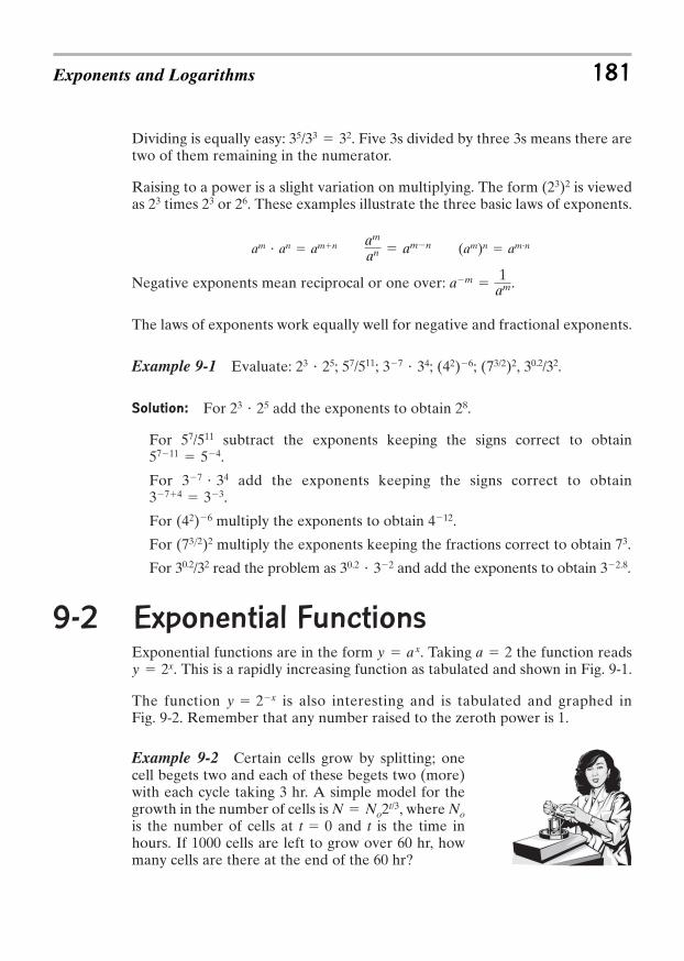
Dividing is equally easy: . Five 3s divided by three 3s means there aretwo of them remaining in the numerator.
Raising to a power is a slight variation on multiplying. The form is viewedas times or . These examples illustrate the three basic laws of exponents.
Negative exponents mean reciprocal or one over: .
The laws of exponents work equally well for negative and fractional exponents.
Example 9-1 Evaluate: ; 57/511; ; ; , 30.2/32.
Solution: For add the exponents to obtain .
For 57/511 subtract the exponents keeping the signs correct to obtain.
For add the exponents keeping the signs correct to obtain.
For multiply the exponents to obtain .
For multiply the exponents keeping the fractions correct to obtain .
For 30.2/32 read the problem as and add the exponents to obtain .
9-2 Exponential FunctionsExponential functions are in the form . Taking the function reads
. This is a rapidly increasing function as tabulated and shown in Fig. 9-1.
The function is also interesting and is tabulated and graphed inFig. 9-2. Remember that any number raised to the zeroth power is 1.
Example 9-2 Certain cells grow by splitting; onecell begets two and each of these begets two (more)with each cycle taking 3 hr. A simple model for thegrowth in the number of cells is , where is the number of cells at and t is the time inhours. If 1000 cells are left to grow over 60 hr, howmany cells are there at the end of the 60 hr?
t 0NoN No2t/3
y 2x
y 2xa 2y ax
32.830.2 32
73(73>2)2
412(42)6
374 3337 34
5711 54
2823 25
(73/2)2(42)637 3423 25
am 1
am
(am)n amnam
an amnam an amn
262323(23)2
35/33 32
Exponents and Logarithms 181
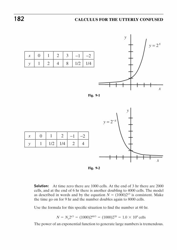
Solution: At time zero there are 1000 cells. At the end of 3 hr there are 2000cells, and at the end of 6 hr there is another doubling to 4000 cells. The modelas described in words and by the equation is consistent. Makethe time go on for 9 hr and the number doubles again to 8000 cells.
Use the formula for this specific situation to find the number at 60 hr.
The power of an exponential function to generate large numbers is tremendous.
N No2t/3 (1000)260/3 (1000)220 1.0 109 cells
N (1000)2t/3
182 CALCULUS FOR THE UTTERLY CONFUSED
Fig. 9-1
x 0 1 2 3 −1 −2
y 1 2 4 8 1/2 1/4
xy 2=
y
x
−xy = 2
y
x
x 1 2 −1 −2
y 1 1/2 1/4 2 4
0
Fig. 9-2
Example 9-3 The return on a certain investment follows ,where R is in dollars when t is in months. How fast is the return declining at thethird month?
Solution: The question concerns a rate and in calculus talk this means the dif-ferential of R with respect to time. So,
The decline in return at 3 months is: .
Example 9-4 The return on $1000 invested in a mining operation producesthe following returns in dollars for the months indicated: R(1) 200, R(2) 165, R(3) 145, R(4) 116, R(5) 86, R(6) 72, R(7) 52, R(8) 50, andR(9) 38. Based on this data, what is the rate the return is declining at the thirdand sixth months?
Solution: An algebra oriented personwould probably take the data for thesecond and fourth months, find theslope symmetric about the third monthand use this as the rate of decline.Captain Calculus would not be contentwith this approach. The Captain wouldplace the data on a spread sheet, havethe spread sheet draw the graph depict-ing the data and calculate the equationdescribing the return over time, andthen differentiate this equation andevaluate it at month three.
The rate equation (from the spread sheet calculation) is
and the derivative is
At month three the rate of decline is
dRdt2t3
3.6(3) 38 $27.20/month
dRdt
3.6t 38
R 1.8t2 38t 238
dRdt2t3
800e0.8(3) ()$72/month
dR 1000e0.8td(0.8t) 800e0.8tdt 1 dRdt
800e0.8t
R(t) 1000e0.8t
Exponents and Logarithms 183
Take me to your spread sheet!
C
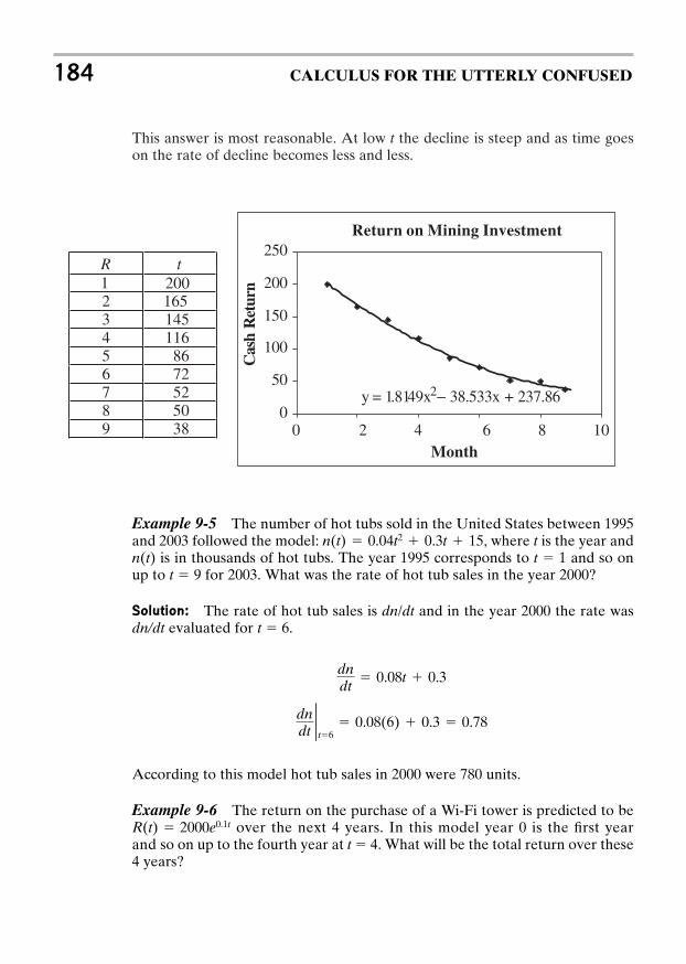
This answer is most reasonable. At low t the decline is steep and as time goeson the rate of decline becomes less and less.
184 CALCULUS FOR THE UTTERLY CONFUSED
R t 1 2002 1653 145 4 116 5 86 6 72 7 52 8 50 9 38
Return on Mining Investment
y = 1.8149x2− 38.533x + 237.860
50
100
150
200
250
0 2 4 6 8 10Month
Cas
h R
etur
n
Example 9-5 The number of hot tubs sold in the United States between 1995and 2003 followed the model: , where t is the year andn(t) is in thousands of hot tubs. The year 1995 corresponds to t 1 and so onup to t 9 for 2003. What was the rate of hot tub sales in the year 2000?
Solution: The rate of hot tub sales is dn/dt and in the year 2000 the rate wasdn/dt evaluated for t 6.
According to this model hot tub sales in 2000 were 780 units.
Example 9-6 The return on the purchase of a Wi-Fi tower is predicted to beover the next 4 years. In this model year 0 is the first year
and so on up to the fourth year at t 4. What will be the total return over these4 years?
R(t) 2000e0.1t
dndt2t6
0.08(6) 0.3 0.78
dndt
0.08t 0.3
n(t) 0.04t2 0.3t 15
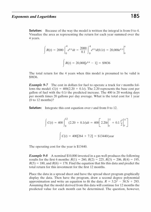
Solution: Because of the way the model is written the integral is from 0 to 4.Visualize the area as representing the return for each year summed over the4 years.
The total return for the 4 years when this model is presumed to be valid is$9836.
Example 9-7 The cost in dollars for fuel to operate a truck for t months fol-lows the model: . The 2.20 represents the base cost pergallon of fuel with the 0.1t the predicted increase. The 400 is 20 working daysper month times 20 gallons per day average. What is the total cost for 1 year(0 to 12 months)?
Solution: Integrate this cost equation over t and from 0 to 12.
The operating cost for the year is $13440.
Example 9-8 A nominal $10,000 invested in a gas well produces the followingresults for the first 6 months: R(1) 260, R(2) 225, R(3) 206, R(4) 195,R(5) 180, and R(6) 178. Find the equation that fits this data and predict thetotal return for this investment for the first 12 months.
Place the data in a spread sheet and have the spread sheet program graphicallydisplay the data. Then have the program, draw a second degree polynomialapproximation and write an equation to fit the data. .Assuming that the model derived from this data will continue for 12 months thepredicted value for each month can be determined. The question, however,
R 3.2t2 38.5t 293
3C(t) 400[264 7.2] $13440/year
3C(t) 400 312
0(2.20 0.1t)dt 400B2.20t 2 12
0 0.1 t2
22 12
0R
C(t) 400(2.20 0.1t)
3R(t) 20,000[e0.4 1] $9836
3R(t) 2000 34
0e0.1tdt
20000.1 3
4
0e0.1td(0.1t) 20,000e0.1t 2 4
0
Exponents and Logarithms 185
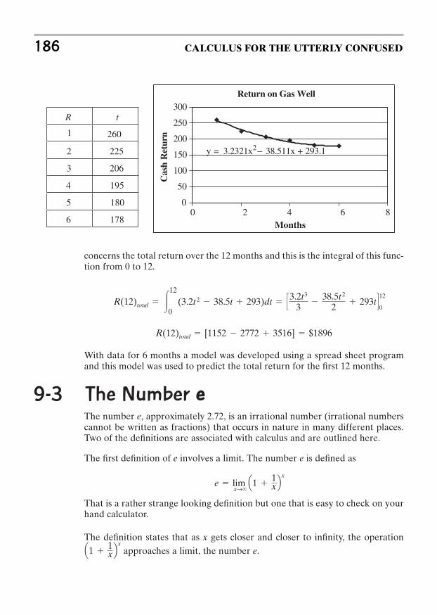
concerns the total return over the 12 months and this is the integral of this func-tion from 0 to 12.
With data for 6 months a model was developed using a spread sheet programand this model was used to predict the total return for the first 12 months.
9-3 The Number eThe number e, approximately 2.72, is an irrational number (irrational numberscannot be written as fractions) that occurs in nature in many different places.Two of the definitions are associated with calculus and are outlined here.
The first definition of e involves a limit. The number e is defined as
That is a rather strange looking definition but one that is easy to check on yourhand calculator.
The definition states that as x gets closer and closer to infinity, the operationapproaches a limit, the number e.Q1
1xR
x
e limxS`
Q1 1xR
x
R(12)total [1152 2772 3516] $1896
R(12)total 312
0(3.2t 2 38.5t 293)dt S
3.2t3
3 38.5t 2
2 293tT12
0
186 CALCULUS FOR THE UTTERLY CONFUSED
R t
260
2 225
3 206
4 195
5 180
6 178
Return on Gas Well
y = 3.2321x2 − 38.511x + 293.1
0
50
100
150
200
250
300
0 2 4 6 8Months
Cas
h R
etur
n1
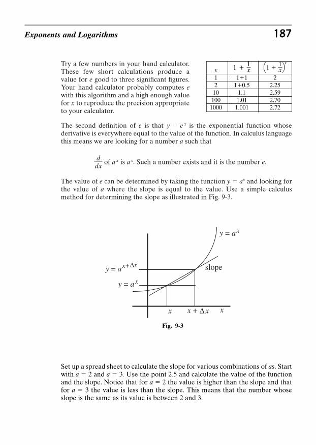
Try a few numbers in your hand calculator.These few short calculations produce avalue for e good to three significant figures.Your hand calculator probably computes ewith this algorithm and a high enough valuefor x to reproduce the precision appropriateto your calculator.
The second definition of e is that is the exponential function whosederivative is everywhere equal to the value of the function. In calculus languagethis means we are looking for a number a such that
of a x is ax. Such a number exists and it is the number e.
The value of e can be determined by taking the function y ax and looking forthe value of a where the slope is equal to the value. Use a simple calculusmethod for determining the slope as illustrated in Fig. 9-3.
ddx
y e x
Exponents and Logarithms 187
y = ax
y = a +x ∆x
x + ∆xx x
y = ax
slope
Fig. 9-3
Set up a spread sheet to calculate the slope for various combinations of as. Startwith a 2 and a 3. Use the point 2.5 and calculate the value of the functionand the slope. Notice that for a 2 the value is higher than the slope and thatfor a 3 the value is less than the slope. This means that the number whoseslope is the same as its value is between 2 and 3.
x1 11 22 10.5 2.2510 1.1 2.59100 1.01 2.701000 1.001 2.72
Q1 1xR
x1
1x
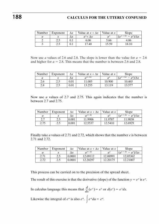
Now use a values of 2.6 and 2.8. The slope is lower than the value for a 2.6and higher for a 2.8. This means that the number is between 2.6 and 2.8.
188 CALCULUS FOR THE UTTERLY CONFUSED
Number Exponent ∆x Value at x + ∆x Value at x Slopea x ∆x ax+ ∆x ax (a x + ∆x ax)/∆x2 2.5 0.1 6.06 5.66 4.063 2.5 0.1 17.40 15.59 18.10
Number Exponent ∆x Value at x + ∆x Value at x Slopea x ∆x ax+ ∆x ax (ax + ∆x ax)/∆x
2.6 2.5 0.01 11.005 10.900 10.4652.8 2.5 0.01 13.255 13.119 13.577
Now use a values of 2.7 and 2.75. This again indicates that the number isbetween 2.7 and 2.75.
Number Exponent ∆x Value at x + ∆x Value at x Slopea x ∆x ax+ ∆x ax (ax + ∆x ax)/∆x
2.7 2.5 0.001 11.9906 11.9787 11.90382.75 2.5 0.001 12.5537 12.5410 12.6929
Finally take a values of 2.71 and 2.72, which shows that the number e is between2.71 and 2.72.
Number Exponent ∆x Value at x + ∆x Value at x Slopea x ∆x ax+ ∆x ax (ax + ∆x ax)/∆x
2.71 2.5 0.0001 12.09112 12.08991 12.053622.72 2.5 0.0001 12.20297 12.20175 12.21007
This process can be carried on to the precision of the spread sheet.
The result of this exercise is that the derivative (slope) of the function y e x is e x.
In calculus language this means that or .
Likewise the integral of is also . .3 e udu eueueu
d(ex) e xdxddx
(e x) ex
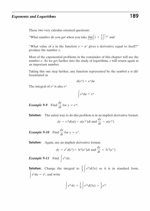
These two very calculus oriented questions:
“What number do you get when you take ?” and
“What value of a in the function gives a derivative equal to itself?”produce the number e.
Most of the exponential problems in the remainder of this chapter will use thenumber e. As we get further into the study of logarithms, e will return again asan important number.
Taking this one step further, any function represented by the symbol u is dif-ferentiated as
The integral of is also
Example 9-9 Find for .
Solution: The safest way to do this problem is in an implicit derivative format.
and
Example 9-10 Find for .
Solution: Again, use an implicit derivative format.
and
Example 9-11 Find .
Solution: Change the integral to so it is in standard form,
, and write
3 e3xdx 13 3 e3xd(3x)
13 e3x
3 eudu eu
13 3 e3xd(3x)
3 e3xdx
dydt
3t 2(e t 3)dy et 3d(t 3) 3t 2(et 3)dt
y e t 3dydt
dydt
a(e at)dy e atd(at) a(e at)dt
y eatdydt
3 eudu eu
eueu
d(eu) e udu
y ax
limxS`
Q1 1xR
x
Exponents and Logarithms 189
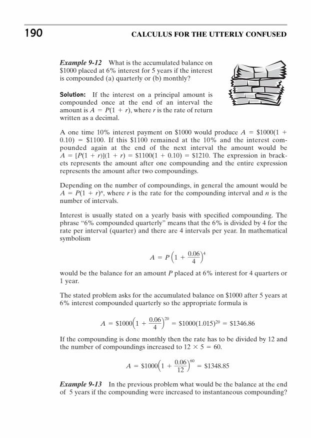
Example 9-12 What is the accumulated balance on$1000 placed at 6% interest for 5 years if the interestis compounded (a) quarterly or (b) monthly?
Solution: If the interest on a principal amount iscompounded once at the end of an interval theamount is , where r is the rate of returnwritten as a decimal.
A one time 10% interest payment on $1000 would produce A $1000(1 0.10) $1100. If this $1100 remained at the 10% and the interest com-pounded again at the end of the next interval the amount would be
. The expression in brack-ets represents the amount after one compounding and the entire expressionrepresents the amount after two compoundings.
Depending on the number of compoundings, in general the amount would be, where r is the rate for the compounding interval and n is the
number of intervals.
Interest is usually stated on a yearly basis with specified compounding. Thephrase “6% compounded quarterly” means that the 6% is divided by 4 for therate per interval (quarter) and there are 4 intervals per year. In mathematicalsymbolism
would be the balance for an amount P placed at 6% interest for 4 quarters or1 year.
The stated problem asks for the accumulated balance on $1000 after 5 years at6% interest compounded quarterly so the appropriate formula is
If the compounding is done monthly then the rate has to be divided by 12 andthe number of compoundings increased to .
Example 9-13 In the previous problem what would be the balance at the endof 5 years if the compounding were increased to instantaneous compounding?
A $1000Q1 0.0612R
60 $1348.85
12 5 60
A $1000Q1 0.06
4 R20
$1000(1.015)20 $1346.86
A P Q1 0.06
4 R4
A P(1 r)n
A [P(1 r)](1 r) $1100(1 0.10) $1210
A P(1 r)
190 CALCULUS FOR THE UTTERLY CONFUSED
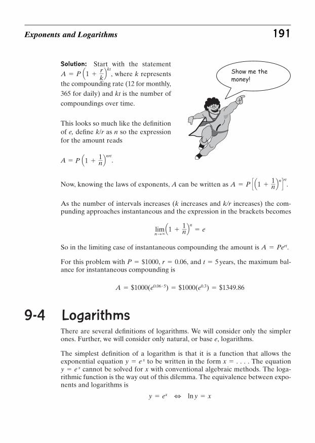
Solution: Start with the statement, where k represents
the compounding rate (12 for monthly,365 for daily) and kt is the number ofcompoundings over time.
This looks so much like the definitionof e, define as n so the expressionfor the amount reads
A .
Now, knowing the laws of exponents, A can be written as .
As the number of intervals increases (k increases and k/r increases) the com-punding approaches instantaneous and the expression in the brackets becomes
So in the limiting case of instantaneous compounding the amount is .
For this problem with , , and , the maximum bal-ance for instantaneous compounding is
9-4 LogarithmsThere are several definitions of logarithms. We will consider only the simplerones. Further, we will consider only natural, or base e, logarithms.
The simplest definition of a logarithm is that it is a function that allows theexponential equation to be written in the form x . . . . The equation
cannot be solved for x with conventional algebraic methods. The loga-rithmic function is the way out of this dilemma. The equivalence between expo-nents and logarithms is
3 ln y xy ex
y e xy e x
A $1000(e0.06 5) $1000(e0.3) $1349.86
t 5 yearsr 0.06P $1000
A Pert
limnS`
Q1 1nR
n e
A P S Q1 1nR
nTrt
P Q1 1nR
nrt
k/r
A P Q1 rkR
kt
Exponents and Logarithms 191
Show me the money!
C
Although there are exponential equations other than base e, most of the expo-nential and logarithmic functions you encounter will be base e. Your hand cal-culator uses base e and base 10, though base 10 is used rarely. The notation ln,as opposed to log, specifies base e. The logarithmic equation just above is readas “log base e” or “ln e” or simply “log” with the later presuming that if the basewere other than e it would be specified.
Run a few numbers on your calculator to become familiar with taking loga-rithms and calculating with exponents. This is not something you do every dayand you don’t want to make a calculating mistake on a test.
On your hand calculator raise e to a power, then take the ln of that number toreturn to the original power (number). [ ] As you go throughthe problems in this chapter keep your calculator handy and practice “punch-ing the numbers.”
Example 9-14 Solve the equations and .
Solution: The equation has to be switched to a logarithmic one:with .
The equation has to be switched to an exponential one: with.u 4.06
u e1.4ln u 1.4
x 1.95x ln 77 ex
ln u 1.47 e x
e3 20; ln20 3
192 CALCULUS FOR THE UTTERLY CONFUSED
Quick Tip
The key phrase to remember in switching from an exponential equation to a log-
arithmic equation and vice versa is “a logarithm is an exponent.” The logarithm
of something is a number and that number is the exponent of e.
I always sing better on a natural log.
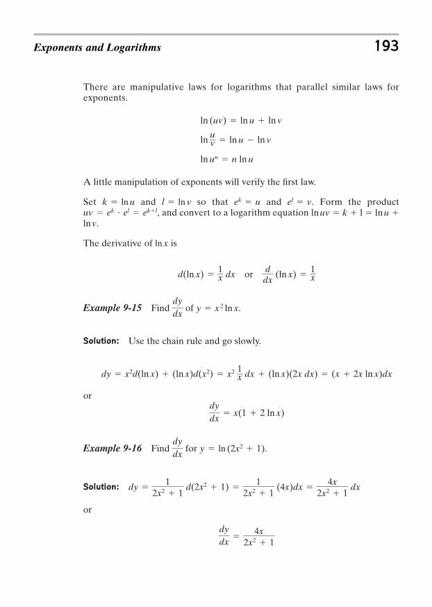
There are manipulative laws for logarithms that parallel similar laws forexponents.
A little manipulation of exponents will verify the first law.
Set and so that and . Form the product, and convert to a logarithm equation lnuv k l lnu
lnv.
The derivative of is
or
Example 9-15 Find of .
Solution: Use the chain rule and go slowly.
or
Example 9-16 Find for .
Solution:
or
dydx
4x
2x2 1
dy 1
2x2 1d(2x2 1)
12x2 1
(4x)dx 4x
2x2 1dx
y ln (2x2 1)dydx
dydx
x(1 2 ln x)
dy x2d(ln x) (ln x)d(x2) x2 1x dx (ln x)(2x dx) (x 2x ln x)dx
y x 2 ln xdydx
ddx
(ln x) 1xd(ln x)
1x dx
ln x
uv ek el eklel vek ul ln vk ln u
ln (uv) ln u ln v
ln uv ln u ln v
ln un n ln u
Exponents and Logarithms 193
Example 9-17 Find the derivative of .
Solution: This looks bad. But, if you proceed slowly, applying the rules one ata time, the differentiation is not all that difficult. The hard part is proceedinglogically. This is a product so write
The differential of is .
The differential of is . Putting it all together we write
or
Example 9-18 Find the derivative of .
Solution: This is a product. Proceed methodically and the problem is not difficult.
There is a simple rule for differentiating logarithmic functions that some authorsuse.
If then .
This is equivalent to using the chain derivative approach and the derivative ofa logarithm as defined in the Mathematical Tables.
Verify for yourself that the two forms are equivalent by working Example 9-15both ways.
Integration of the logarithmic function follows , which isused so rarely that we only give this one example.
3 ln x dx x ln x x
dy 1
f(x)d( f(x))
dydx
ddx
( f(x))
f(x)y ln f(x)
dydx
ex( cos x sin x)
dy exd( sin x) sin xd(ex) ex( cos x)dx ex( sin x)dx
y ex sin x
dydx
2x2.5
x2 2 1.5x 0.5 ln (x2 2)dy x1.5 2xdx
x2 2 1.5x 0.5 ln (x2 2)dx
1.5x 0.5dxx1.5
1x2 2
d(x2 2) 2xdx
x2 2ln (x2 2)
dy x1.5d[ln (x2 2)] ln (x2 2)dx1.5
y x1.5 ln (x2 2)
194 CALCULUS FOR THE UTTERLY CONFUSED
Example 9-19 Find .
Solution:
9-5 Growth and Decay ProblemsThe growth and decay model is appropriate to many phenomena, such seem-ingly diverse problems as population growth, radioactive decay, the spread ofdisease, the cooling of a cup of coffee, and the num-ber of yeast in a culture, just to name a few. Beforeworking some problems, a very simple model of bac-teria or yeast growth will be developed and workedthrough in detail. Notice the pattern in the problem.Many mathematical models of different phenomenaparallel this one.
A simple experiment performed in elementarychemistry, biology, or physical science courses is thegrowth of bacteria or yeast. In this experiment a cer-tain number (the number is often determined ormeasured by weight) of bacteria are placed in a nutrient environment. Thismeans that the bacteria have optimum growing conditions, food, temperature,and the like. Their growth is then limited by their growth mechanism and notby anything external.
The bacteria grow by budding, one bacterium grows on another, splitting, eachbacterium divides producing two identical bacteria, so that each bacterium overan average time period becomes two bacteria and these two repeat the sameprocess in the same time period and on and on. At any time in the process thenumber of bacteria produced per unit of time is proportional to the numberpresent. This is the mathematical statement of the growth model for bacteria.In symbolic form, , the number produced per unit of time is proportionalto the number present, .
Solving this statement for N as a function of time is a calculus problem, and onewe already have some experience with.
In practical terms the difficulty with the rate statement is that the N is on thewrong side of the equation. It needs to be associated with the dN if we are to
dNdt
kN
kNdN/dt
y 12 3 ln 2x d(2x) 2x ln 2x 2x
y 3 ln 2x dx
Exponents and Logarithms 195
make any progress toward a solution. A little algebra fixes this.
Now integrate both sides of the equation. (Remember:
)
3
The constant is required because there are no limits on the integrals.
In this problem, as with every problem in growth or decay, there is an initialamount of material. In this case there is an initial number of bacteria at the startof the experiment. Call this initial amount . In the language of mathematics,at , . Substitute these values into .
so
With the constant evaluated in terms of the initial amount of material the basicrelation is
or or
If you had any trouble manipulating the logarithms in the previous line, go backand review the manipulative rules for logarithms. At this point switch to anexponential format.
3 or
This last statement correctly describes the model. The number of bacteria atany time starts out at ( ) and increases with time in an exponentialmanner.
This is the general growth law for something with growth propor-tional to the number present. Some text authors begin the discussion of growthand decay with this equation. This approach is simple but neglects the develop-ment of a mathematical model of a simple statement that “the growth of . . . isproportional to the number of . . . present at any time.” A little reflection willconvince you that this model fits many different phenomena.
Suppose in this bacteria growth problem that 100 bacteria are introduced intoa growth environment (water, nutrients, and the like) and that 2 hr later the
N Noekt
e0 1No
N Noe ktNNo
ektlnNNo
kt
lnNNo
ktln N ln No ktln N kt ln No
C ln Noln No k(0) C
ln N kt CN Not 0No
ln N kt C3 dNN 3 kdt
so 3 dxx ln x
3 d(ln x) 3 dxx
dNN kdt
196 CALCULUS FOR THE UTTERLY CONFUSED

bacteria are separated from the environment or otherwise identified and thattheir number has increased to 130. Can this information be used to determinethe growth law?
With these two numbers, N and , and the time interval the constant k can beevaluated. The calculation is a little logarithm and exponent intense but followalong with your calculator. Substitute as follows:
or
To solve for k switch to a logarithmic equation. (Remember: “A log-arithm is an exponent.”) The logarithm of something is an exponent so
or
The specific law governing the growth of these bacteria in this environment is
With this law it is possible to predict how many of these bacteria would be pres-ent, say, after 12 hr and starting with 50 bacteria. Put in the 50 for and the 12 hrfor t and we get
This model that starts with the statement that the growth rate is proportional tothe amount present can, with a modest amount of calculus and initial informa-tion, be used to predict future growth.
There is a standard pattern to growth and decay problems that always works.The general procedure for these problems is outlined below.
1. Any problem where the number of events is proportional to the number ofparticipants present can be written as equals a constant (+k for
growth and for decay) times the number: .
2. Rearrange to and integrate to get ln N
kt + N0. Take an initial number , at , to evaluate , and
write lnN kt + lnNo.
3. Rearrange the equation to and switch to an exponential format
or .N NoektNNo
ekt
lnNNo
kt
A ln Not 0No
3 dNN k 3 dtdN
N kdt
dNdt
kNk
dN/dt
N 50e0.13 12 50(4.76) 238
No
N Noe 0.13t
k 12 ln 1.30 0.13ln 1.30 2k
1.30 e 2k
1.30 e 2k130 100e 2k
No
Exponents and Logarithms 197
4. One data point, a certain N at a specific time, allows calculation of k. (Forexample, a 20% increase in in 1 hr means or .Switch to a logarithmic equation and and finally write
.)
5. With the calculation of k, the specific growth or decay equation is writtenfor the same conditions that produced the initial data. With this specificgrowth or decay equation N at any time can be predicted.
Refer to this procedure in subsequent problems. It is a very logical procedurefor growth and decay problems and it works. Growth and decay problems arefavorite test problems. Know how to work them and especially know how toswitch from exponential equations to logarithmic equations and vice versa andknow how to take logs and perform exponentiation on your hand calculator.
Example 9-20 If “a fool and his money are soon parted,” the rate at which itleaves is probably proportional to the amount remaining. If a certain fool start-ing with $20,000 starts gambling his money away and after 2 hr has lost $2000,how long will it take for him to loose 90% of the original amount?
Solution: The basic assumption in this problem isthat the fool will loose in proportion to the amounthe has at any time. Humans are a little harder topredict than bacteria, but this is a good assumption.Follow the procedural steps as written previouslyand be aware of the logic in the problem.
Step 1: The statement “the rate at which the foollooses money is proportional to the amount pres-ent” means that
Step 2: Rearrange, integrate, and evaluate the constant of integration with theinitial data.
,
At t 0, the fool has $20,000, so ln20,000 k(0) + C and C ln20,000.
Now the equation reads
ln A kt ln 20,000
ln A kt CdAA
kdt, 3 dAA
k 3 dt
dAdt
kA
N Noe0.18tk ln 1.2 0.18
1.2 e1k1.2No Noe1kNo
198 CALCULUS FOR THE UTTERLY CONFUSED
Step 3: Rearrange and switch to exponents.
, and switching to exponents or .
Step 4: Use the given data to determine k.At , A has declined to 18,000, so put these numbers into the amountstatement and find k.
,
Switch to logarithms to solve this equation for k.
, k ln (0.9)
2 0.0532k ln (0.9)
0.9 e2k18,000 2000e2k
t 2 hrs
A 20,000ektA20,000 ektln A
20,000 kt
Exponents and Logarithms 199
As you were following along this problem and “punching the numbers,” soyou would be very proficient at this logarithm and exponent calculating forthe test on this topic, you may have noticed that your calculator displayed anegative number for ln(0.9). This is correct. In the original statement of theproblem, so that the calculation of k should produce a posi-tive number. The reason for the ln of numbers less than 1 being negative hasto do with one of those other definitions of the ln and will be taken up shortly.
dA/dt kA
Step 5: The specific equation for this situation is .
The time for 10% remaining is the time for A to reach 2000. Substitute forand solve for t.
,
Switching to logarithms, or .
Based on this model, it would take this particular fool 43 hr to loose 90% of anoriginal amount of $20,000.
Example 9-21 Hot or cold objects cool down or heat up to the temperatureof their surroundings. The temperature difference, , between the object andits surroundings decreases over time in proportion to that temperature differ-ence. This is Newton’s law of cooling. If a cup of coffee cools from to 80C85C
T
t 1
0.053 ln (0.1) 43 hrsln (0.1) 0.053t
0.1 e0.053t2000 20,000e0.53t
A 2000
A 20,000e0.053t
in 2 minutes in room temperature surroundings, how long does it take for thecoffee to cool from to ( is room temperature)?
Solution: Don’t be fooled by the wording of this problem.It is not the temperature that is important, but the differencein temperature between the coffee and its surroundings.The definitive statement is “the change in the temperaturedifference is proportional to the difference.” Call the dif-ference in temperature between the coffee and its surround-ings. The mathematical statement of Newton’s law of coolingthen is
Rearrange and integrate.
When the coffee starts cooling, the temperature difference is 65C (85 20)Cso and so the equation becomes
or
Switching to exponents we write
or
Be careful with this next step. The temperature changes by 5C so the temper-ature difference is now 60C, and this occurs over 2 min so put in these valuesand evaluate k.
, , and switching to logarithms
, k 12 ln 60
65 0.042k ln 60
65
6065
e2k60 65e2k
T 65ekt T65
ekt
ln T65
ktln ( T ) kt ln 65
C ln 65ln 65 k(0) C
d( T) T
kdt, 3 1 T
d( T ) k 3 dt, ln( T ) kt C
d( T)dt
k( T )
T
20C30C85C
200 CALCULUS FOR THE UTTERLY CONFUSED
The temperature difference statement is now
Be careful again. Go back and read the question and make sure you understandthat the desired time is for the temperature to reach a 10C difference betweenthe coffee and its surroundings. Use the 10C temperature difference and cal-culate the time.
, , ,
It takes 47 min for this cup of coffee to cool to within of room temperature.
Example 9-22 A wildlife manager needs to reach a 10,000 population ofmule-eared deer in a certain habitat in 6 years. There are presently no deer inthe habitat. The environment is such that the deer can grow without being lim-ited by their environment. This means that the growth of the deer populationwill be proportional to the population, . In order to determine thegrowth equation, 100 deer are introduced into the habitat. There are half malesand half females, the same ratio as when they reproduce. At the end of the yearthere are 130 deer. How many deer need to be introduced to the habitat toachieve the 10,000 goal in the remaining 5 years?
Solution: The first part of the problem is to determine the growth equation.Starting with
, the general growth equation is
The 100 deer population grows to 130 in 1 year so put this data into and determine k.
or so that on switching, or
The specific growth law for these deer in this habitat is . Now solvefor the initial number needed to produce the 10,000 population in 5 moreyears.
or
This number minus the 130 already there, or , deer need tobe introduced to achieve the 10,000 goal in the prescribed time.
2725 130 2595
Po 272510,000 Poe0.26?5 Poe1.30 3.67Po
Po
P Poe0.26t
k 0.26ln 1.30 k1.30 e1k130 100e1k
P Poekt
P PoektdPdt
kP
dP/dt kP
10 C
t 1
0.04 ln 1065
47 minutes0.04t ln 1065
1065
e0.04t10 65e0.04t
T 65e0.04t
Exponents and Logarithms 201
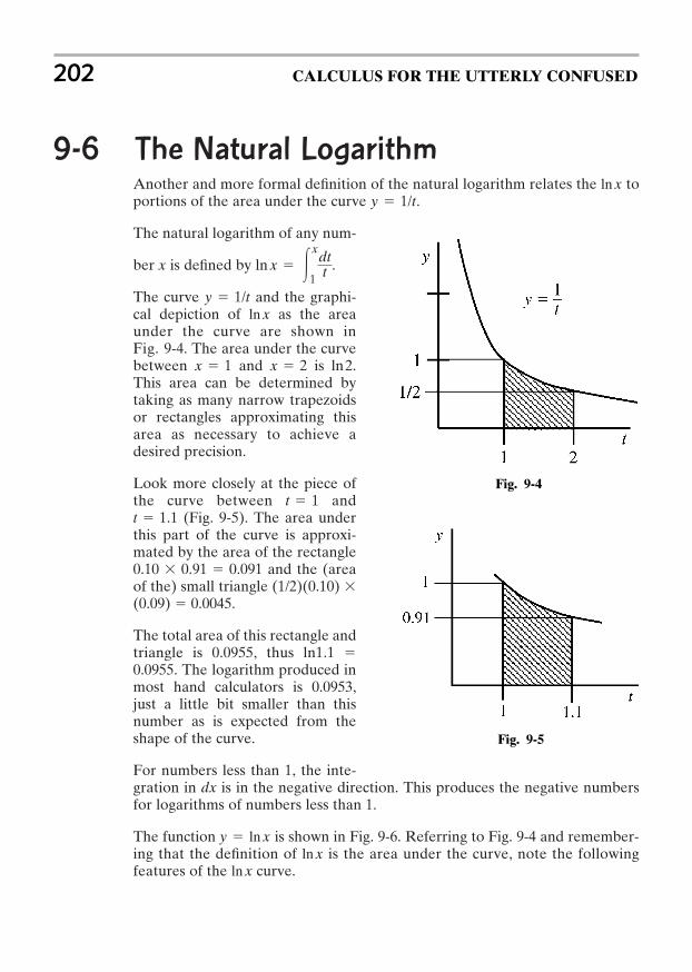
9-6 The Natural LogarithmAnother and more formal definition of the natural logarithm relates the toportions of the area under the curve .
The natural logarithm of any num-
ber x is defined by .
The curve and the graphi-cal depiction of as the areaunder the curve are shown inFig. 9-4. The area under the curvebetween and is ln2.This area can be determined bytaking as many narrow trapezoidsor rectangles approximating thisarea as necessary to achieve adesired precision.
Look more closely at the piece ofthe curve between and
(Fig. 9-5). The area underthis part of the curve is approxi-mated by the area of the rectangle
and the (areaof the) small triangle (1/2)(0.10) (0.09) 0.0045.
The total area of this rectangle andtriangle is 0.0955, thus ln1.1 0.0955. The logarithm produced inmost hand calculators is 0.0953,just a little bit smaller than thisnumber as is expected from theshape of the curve.
For numbers less than 1, the inte-gration in dx is in the negative direction. This produces the negative numbersfor logarithms of numbers less than 1.
The function is shown in Fig. 9-6. Referring to Fig. 9-4 and remember-ing that the definition of is the area under the curve, note the followingfeatures of the curve.ln x
ln xy ln x
0.10 0.91 0.091
t 1.1t 1
x 2x 1
ln xy 1/t
ln x 3x
1
dtt
y 1/tln x
202 CALCULUS FOR THE UTTERLY CONFUSED
Fig. 9-4
Fig. 9-5
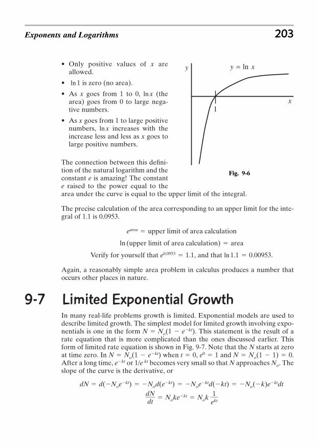
• Only positive values of x areallowed.
• is zero (no area).
• As x goes from 1 to 0, (thearea) goes from 0 to large nega-tive numbers.
• As x goes from 1 to large positivenumbers, increases with theincrease less and less as x goes tolarge positive numbers.
The connection between this defini-tion of the natural logarithm and theconstant e is amazing! The constante raised to the power equal to thearea under the curve is equal to the upper limit of the integral.
The precise calculation of the area corresponding to an upper limit for the inte-gral of 1.1 is 0.0953.
Verify for yourself that , and that .
Again, a reasonably simple area problem in calculus produces a number thatoccurs other places in nature.
9-7 Limited Exponential GrowthIn many real-life problems growth is limited. Exponential models are used todescribe limited growth. The simplest model for limited growth involving expo-nentials is one in the form . This statement is the result of arate equation that is more complicated than the ones discussed earlier. Thisform of limited rate equation is shown in Fig. 9-7. Note that the N starts at zeroat time zero. In when , and .After a long time, or becomes very small so that N approaches . Theslope of the curve is the derivative, or
dNdt
Nokekt Nok 1ekt
dN d(Noekt) Nod(ekt) Noektd(kt) No(k)ektdt
No1/e ktektN No(1 1) 0e0 1t 0N No(1 ekt)
N No(1 ekt)
ln 1.1 0.00953e0.0953 1.1
ln (upper limit of area calculation) area
earea upper limit of area calculation
ln x
ln x
ln 1
Exponents and Logarithms 203
1x
y xy ln=
Fig. 9-6
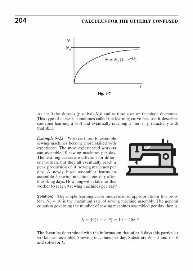
At the slope is (positive) and as time goes on the slope decreases.This type of curve is sometimes called the learning curve because it describessomeone learning a skill and eventually reaching a limit in productivity withthat skill.
Example 9-23 Workers hired to assemblesewing machines become more skilled withexperience. The most experienced workerscan assemble 10 sewing machines per day.The learning curves are different for differ-ent workers but they all eventually reach apeak production of 10 sewing machines perday. A newly hired assembler learns toassemble 5 sewing machines per day after6 working days. How long will it take for thisworker to reach 9 sewing machines per day?
Solution: The simple learning curve model is most appropriate for this prob-lem. is the maximum rate of sewing machine assembly. The generalequation governing the number of sewing machines assembled per day then is
The k can be determined with the information that after 6 days this particularworker can assemble 5 sewing machines per day. Substitute and and solve for k.
t 6N 5
N 10(1 ekt) 10 10ekt
No 10
Nokt 0
204 CALCULUS FOR THE UTTERLY CONFUSED
)1( kto eNN =
t
oN
N
− −
Fig. 9-7
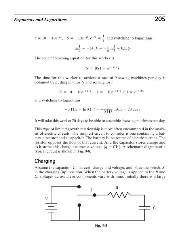
, , , and switching to logarithms
,
The specific learning equation for this worker is
The time for this worker to achieve a rate of 9 sewing machines per day isobtained by putting in 9 for N and solving for t.
, ,
and switching to logarithms
,
It will take this worker 20 days to be able to assemble 9 sewing machines per day.
This type of limited growth relationship is most often encountered in the analy-sis of electric circuits. The simplest circuit to consider is one containing a bat-tery, a resistor and a capacitor. The battery is the source of electric current. Theresistor opposes the flow of that current. And the capacitor stores charge andas it stores this charge assumes a voltage (q CV ). A schematic diagram of atypical circuit is shown in Fig. 9-8.
Charging
Assume the capacitor, C, has zero charge and voltage, and place the switch, S,in the charging (up) position. When the battery voltage is applied to the R andC, voltages across these components vary with time. Initially there is a large
t 1
0.115 ln 0.1 20 days0.115t ln 0.1
0.1 e0.115t1 10e0.115t9 10 10e0.115t
N 10(1 e0.115t)
k 16
ln 12 0.115ln 1
2 6k
e6k 125 10e6k5 10 10e6k
Exponents and Logarithms 205
V
R
C
S
Fig. 9-8
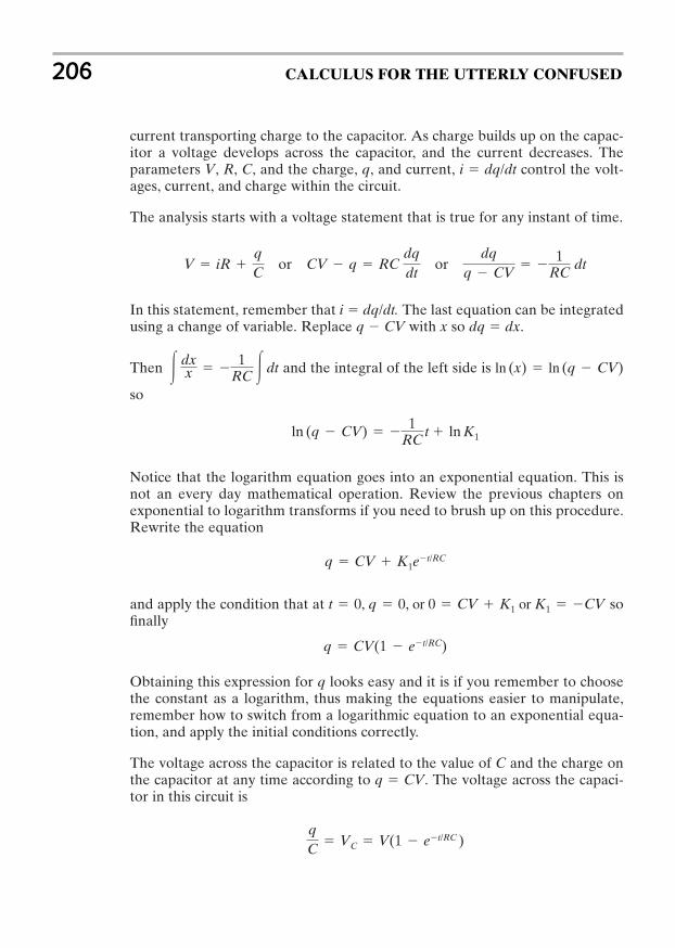
current transporting charge to the capacitor. As charge builds up on the capac-itor a voltage develops across the capacitor, and the current decreases. Theparameters V, R, C, and the charge, q, and current, i dq/dt control the volt-ages, current, and charge within the circuit.
The analysis starts with a voltage statement that is true for any instant of time.
In this statement, remember that i dq/dt. The last equation can be integratedusing a change of variable. Replace q CV with x so dq dx.
Then and the integral of the left side is
so
Notice that the logarithm equation goes into an exponential equation. This isnot an every day mathematical operation. Review the previous chapters onexponential to logarithm transforms if you need to brush up on this procedure.Rewrite the equation
and apply the condition that at sofinally
Obtaining this expression for q looks easy and it is if you remember to choosethe constant as a logarithm, thus making the equations easier to manipulate,remember how to switch from a logarithmic equation to an exponential equa-tion, and apply the initial conditions correctly.
The voltage across the capacitor is related to the value of C and the charge onthe capacitor at any time according to q CV. The voltage across the capaci-tor in this circuit is
qC
VC V(1 et/RC )
q CV(1 et/RC)
t 0, q 0, or 0 CV K1 or K1 CV
q CV K1et/RC
ln (q CV) 1
RCt ln K1
ln (x) ln (q CV)3 dxx
1RC 3 dt
V iR qC or CV q RC
dqdt
or dq
q CV
1RC
dt
206 CALCULUS FOR THE UTTERLY CONFUSED
The current in the resistor is
The voltage across the resistor is
There are two graphs that are helpful in understanding the situation: one isq vs. t, and the other is i vs. t. These are shown in Fig. 9-9.
VR iR Vet/RC
i dqdt
VR et/RC
Exponents and Logarithms 207
tt
q i
CV V/R
Fig. 9-9
Notice in the curve of q v.s t, that at t 0, q 0, and as
In the curve of i vs. t, at t 0, i V/R, and as .
At t 0 the charge on the capacitor is zero and the current is maximum and ast goes to infinity the current goes to zero and the charge reaches its maximumof CV.
The Time Constant
In biological systems that grow exponentially the systems are often character-ized by giving the doubling time, the time for the system to double in number,size, or mass. In electrical systems that grow exponentially the systems are char-acterized by a time constant, the time to make the exponent of e equal to 1. Thetime constant for this circuit is RC.
Look at the equation above and the q vs. t graph. When and the charge on the capacitor has risen to 0.63 of its final value. A similar
t RC, 1 e1 0.63
t S `, i S 0
t S `, q S CV.
statement can be made about the voltage on the capacitor. After one time con-stant, the voltage on the capacitor is 0.63 of the battery voltage.
The current, meanwhile, has in one time constant dropped to of itsinitial value.
Example 9-24 A resistor and a capacitor are placed in series witha battery as shown in Fig. 9-8. Find the charge on the capacitor, the cur-rent, and the voltages on the capacitor and resistor at the instant the switch isclosed, .
Solution: At the charge on the capacitor is zero.
At , the current is .
At , the voltage on the capacitor is zero (it has no charge) and the entirebattery voltage of is across the resistor.
Example 9-25 For the circuit of the previous problem, find the time constant,and the charge, current, and VR, and VC at a time equal to one time constant.
Solution: The time constant is . Thecharge on the capacitor at t 0.20 s is
The current at t 0.20s is
The voltage across the capacitor is .The voltage across the resistor is .
These problems can be deceptively easy. Be sure you know how to manipulatethe exponents on your calculator. Don’t get a test problem wrong because youdid not practice all the steps in the problem and were unfamiliar with manipu-lating exponents on your calculator.
Example 9-26 For the circuit of the previous two problems, how long does ittake for the capacitor to reach 80% of its final charge?
12 V 7.6 V 4.4 VVC V(1 e1) 12 V 0.63 7.6 V
i ZtRC VR e1
12 V1.0 104
0.37 4.4 104A
q ZtRC CV(1 e1) 12 V(20 106F)0.63 1.5 104C
RC 10 103 20 106F 0.20 s
12 Vt 0
i V/R 12 V/10 103 1.2 103 At 0
t 0
t 0
12 V20mF10 k
e1 0.37
208 CALCULUS FOR THE UTTERLY CONFUSED
Solution: This problem is similar to radioactive decay problems where wewant to know the time for half the material to decay. There is a fair amount ofalgebraic manipulation that is easier to follow without numbers, so the problemwill be worked as far as possible with symbols.
Start with and note that the final (fully charged) q is equalto CV. Mathematically, when
To find the time for 80% charge set q equal to 80% of the final charge, or, and solve for t.
For convenience switch to positive exponents so
In order to solve for t, switch the exponential equation to a logarithmic equa-tion. One of the functions of logarithms is to solve for variables in exponents.
Now put in the values for R and C.
.
As a check note that
Discharging
After the capacitor is left to charge for a long time (many time constants) thecharge is CV. Move the switch to the discharge position (down in Fig. 9-8)where R and C are in series. When the charged capacitor and resistor are placedin series the charged capacitor acts as a battery. The voltage on the capacitor is
, and this voltage appears across the resistor as . As time goes on, thecharge on the capacitor is depleted and the current drops (eventually) to zero.The charge decays according to
and the current according to
i dqdt
ddt
CVet/RC VR et/RC
q CVet/RC
iRq/C
1 et/RC 1 e0.32/0.20 0.80
t RC ln5 1.0 104 20 106F ln5 0.32 s
t/RC ln5 or t RC ln5
1/et/RC 0.20 or et/RC 1/0.20 5
0.80CV CV(1 et/RC) or 080 1 et/RC or et/RC 0.20
q 0.80CV
t S `, et/RC S 0 and 1 et/RC S 1 so q S CV.q CV(1 et/RC)
Exponents and Logarithms 209
The negative sign indicates that the current in the resistor is in the oppositedirection from the charging situation, which must be the case.
Mathematical analysis of the discharge circuit starts with a voltage type ofstatement similar to the one used in the charging case.
and solving
Again notice that the choice of constant is very convenient because
Now impose the initial condition. At
The charge on the capacitor decays with the same time constant, RC.
Example 9-27 If the circuit used in the previous problems is placed in the dis-charge mode, how long does it take for the circuit to discharge to 50% of itsoriginal (total) charge?
Solution: Solve for t when .
It is more convenient to write 0.50 as 1/2, so when the statement is converted tologarithms,
In terms of time constants this would be , (RC)ln2, time constants, or 0.69 ofa time constant.
ln2
t RC ln2 1.0 104 20 106 F ln2 (0.20)(0.69 s) 0.14 s
ln 0.50 t
RC is ln1 ln2
tRC
and since ln1 0
0.50 CV CVet/RC or 0.50 et/RC
q 0.50 CVq CVet/RC
q CVet/RC
t 0, q CV, so K2 CV and
lnq
K2
1RC
t or q
K2 et/RC or q K2e
t/RC
lnq (1/RC) t lnK2
iR qC
0 or dqdt
1
RCq or
dqq
1RC
dt
210 CALCULUS FOR THE UTTERLY CONFUSED
It makes sense that our answer is less than one time constant since it takes lesstime for the charge to decline to 50% of its initial value than to 37% ( ) of itsinitial value.
Example 9-28 An RC circuit is observed during discharge to have an initialcapacitor potential of 100 V and after 3.0 s to have a potential of 20 V. How longwill it take for the capacitor to discharge to 1.0 V.
Solution: The voltage across the capacitor at any time is determined byrewritten as q/C, or , where is the voltage at
.
Take
Switching to logarithms
Knowing this number, the specific decay law for this circuit can be written
Now calculate the time for the voltage to drop to 1.0 V.
Switching to logarithms
Go back over this problem and note the procedure.
1. After reading the problem, the general law (equation) was written down,.
2. Next the data from the problem (100 V going to 20 V in 3.0 s) was used tofind RC.
3. With RC the specific law for this problem was written; .
4. Finally, with this specific law the predictive calculation was performed tofind the time for the 100 V to decay to 1.0 V.
V 100 Vet/1.9
VC Voet/RC
ln 100 (t/1.9) or t 1.9 ln 100 8.6 s
1.0 V 100 Vet/1.9 or (1/100) et/1.9
V (100 V)et/1.9
3.0RC
ln5 or 3.0ln5
RC or RC 1.9 s
20 V 100 Ve3.0/RC or 2/10 e3.0/RC or e3.0/RC 5
Vo 100, VC 20 V, and t 3.0 s and write
t 0VoVC Voet/RCq CVet/RC
1/e
Exponents and Logarithms 211

This analysis procedure is typical of growth and decay problems in general. Befamiliar with the steps in this procedure. It will keep you from getting lost andnot knowing how to proceed in problems like this.
9-8 The Logistic FunctionAnother type of exponential function used to describe limited growth has theform
At , . This is the present rate or number, whatever R represents.
As t goes to infinity, goes to 0 and R approaches B. B is the maxi-mum rate or number.
This curve has the general shape shown in Fig. 9-10.
ekt 1/ekt
R B
1 At 0
R B
1 Aekt
212 CALCULUS FOR THE UTTERLY CONFUSED
B
ktAe
BR
+=
1AB+1
0 t
R
−
Fig. 9-10
Many industries follow this type of a growth curve. When a new product isintroduced there is considerable demand, but as more and more people acquire,the product sales drop to a level determined by the number of new peopleentering the marketplace and replacement of old or outdated product. Theautomobile industry is an excellent example of this type of growth.
The exponential part of the definition is sometimes written as . This form isworkable if data defining the function is available for small values of x. Look at
bx
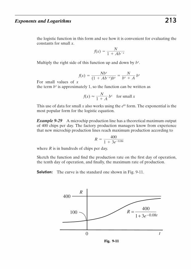
the logistic function in this form and see how it is convenient for evaluating theconstants for small x.
Multiply the right side of this function up and down by .
For small values of xthe term bx is approximately 1, so the function can be written as
This use of data for small x also works using the form. The exponential is themost popular form for the logistic equation.
Example 9-29 A microchip production line has a theoretical maximum outputof 400 chips per day. The factory production managers know from experiencethat new microchip production lines reach maximum production according to
where R is in hundreds of chips per day.
Sketch the function and find the production rate on the first day of operation,the tenth day of operation, and finally, the maximum rate of production.
Solution: The curve is the standard one shown in Fig. 9-11.
R 400
1 3e0.08t
ekt
f(x) < N1 A
bx for small x
f(x) Nbx
(1 Abx)bx N
bx Abx
bx
f(x) N
1 Abx
Exponents and Logarithms 213
400
eR
0.08t31
400
+=
0 t
R
100 _
Fig. 9-11
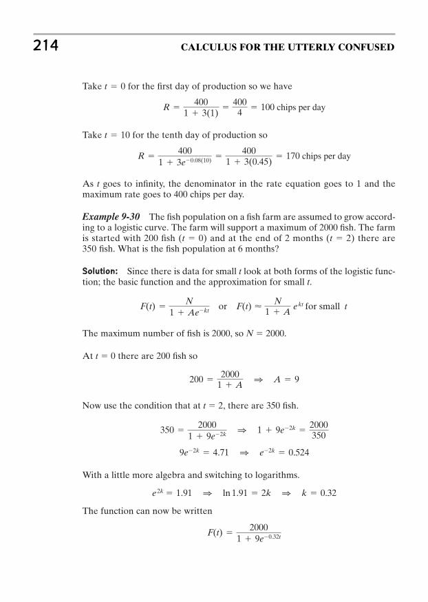
Take for the first day of production so we have
Take for the tenth day of production so
As t goes to infinity, the denominator in the rate equation goes to 1 and themaximum rate goes to 400 chips per day.
Example 9-30 The fish population on a fish farm are assumed to grow accord-ing to a logistic curve. The farm will support a maximum of 2000 fish. The farmis started with 200 fish (t 0) and at the end of 2 months (t 2) there are350 fish. What is the fish population at 6 months?
Solution: Since there is data for small t look at both forms of the logistic func-tion; the basic function and the approximation for small t.
The maximum number of fish is 2000, so N 2000.
At t 0 there are 200 fish so
Now use the condition that at t 2, there are 350 fish.
With a little more algebra and switching to logarithms.
The function can now be written
F(t) 2000
1 9e0.32t
e 2k 1.91 1 ln 1.91 2k 1 k 0.32
9e2k 4.71 1 e2k 0.524
350 2000
1 9e2k 1 1 9e2k 2000350
200 2000
1 A 1 A 9
F(t) N
1 Aekt or F(t) < N1 A
ekt for small t
R 400
1 3e0.08(10) 400
1 3(0.45) 170 chips per day
t 10
R 400
1 3(1)
4004 100 chips per day
t 0
214 CALCULUS FOR THE UTTERLY CONFUSED
and evaluated at the end of 6 months.
fish
Interval and instantaneous compound interest
Know how to differentiate logarithms and exponents
Know how to integrate logarithms and exponents
Differentiate and integrate trigonometric functions
Solve growth and decay problems
Use spread sheets to find rates and predict total returns
Solve limited growth exponentials
Solve problems that fit a logistic model
se spread sheets to find rates and predict total returns * Solve limited growth exponentials
PROBLEMS
1. Differentiate , , and .
2. Integrate , and .
3. An amount of $2000 is invested at 12% with compounding quarterly.Determine how long it takes to grow the $2000 to $5000.
4. The current and voltage in an R-L (resistance and inductor) circuit behavein much the same way as for an R-C circuit. The voltage statement valid at
every instant after the switch is closed is .
Solve this equation for i and di/dt for a 60 V battery connected to a 50 103 Hinductor and a 180 Ω resistor.
5. What is the time constant for the circuit of problem 4?6. Radioactive materials decay in direct proportion to the amount of materi-
al present. Radioactive Polonium decays with a half-life of 140 days. Howmuch of a 300 g sample remains after 360 days. You may want to review theprocedure for growth and decay problems in the text before working thisproblem.
7. For the previous problem how long does it take for 90% of the material todecay?
8. $100,000 invested in an oil well produces the following results for the first6 months: R(1) 2700, R(2) 2150, R(3) 2010, R(4) 1800, R(5) 1760,
V iR L didt
0
3 x 3e x 42dx3 Q3ex 2x
x2
2 Rdx3 x dxx2 1
f(x) (x2 1) ln xf(x) x ln xf(x) ln (x 1)
F(6) 2000
1 9e1.94 872
Exponents and Logarithms 215
and R(6) 1680. Find the equation that fits this data and find the rate ofdecline at R(5).
9. For the previous problem, what is the expected return over the first12 months?
10. The number of pet strollers sold by a certain company in the 1995 to 2003range was with t measured in thousands ofstrollers. The year 1995 corresponds to t 5 and so on up to t 13 for 2003.What was the rate of stroller sales in the year 2000?
11. Use the logistic formula with base e to describe the growth of tattoo parlorsas the industry matures. Assume that a 3 million population metropolis cansupport 200 parlors. In 1990, t 0, there are 6 parlors. In 1993, t 3, thereare 12 parlors. Determine the specific logistic formula and predict the num-ber of parlors in 1996, t 6.
12. Sales of the Supertimewaster video game are following the logistic modelgiven below, where q is the number of games sold per month and t is thetime in months. What is the rate of sales at 10 months?
ANSWERS
1.
.
2. Let
can be integrated with a change of variable. First rewrite the
integral as . With a new variable and
the integral is now so .
3. Start with the statement , where P is the initial amount, r is
the annual rate, k is the compounding interval and t is the number of years.
Enter the numbers and the expression looks like .A ($2000)Q1 0.12
4 R4t
A PQ1 rkR
kt
3 x3ex44dx 14[ex42]1
4 3 eudu eu
du 4x3dxu x4 214 3 4x3ex42dx
3 x 3ex42dx
3ex 2ln Zx Z x3
6
3 xdxx2 1
1 12 3 du
u 12 ln u
12 ln Zx2 1 Zu x2 1 so du 2xdx
df(x) (x2 1) dxx ln x(2xdx) 1
dfdx
x2 1
x 2x ln x
df(x) xd ln x ln xdx 1 dfdx
1 ln x
df(x) 1
x 1d(x 1) 1
dfdx
1
x 1
q(t) 5000
1 2e0.4t
n(t) 0.04t2 0.3t 15
216 CALCULUS FOR THE UTTERLY CONFUSED
Now impose the requirement for A to reach $5000: .With a little manipulation, . This is one of those inocuouslooking equations that can drive you crazy! If the base were e, it would beappropriate to take logarithms. Since the base is 1.03, we need either base1.03 logarithms, a mechanism for switching bases of logarithms, or anothermethod for solving for t. It is possible to switch bases of logarithms but inthis case a few key strokes on a calculator or a spread sheet will solve theproblem nicely. Raise 1.03 to a few powers and find what power produces2.5 to the two significant figures given in the problem. About 10 key strokesand a fraction of a minute produces a number of 31.1 for the exponent 4t soabout 7.8 years are necessary at these conditions to grow $2000 to $5000.
4. The solution is similar to the one for the R-C circuit done in the text. Areview of that more detailed analysis may be helpful before continuing.
Rewrite this equation as .
Switching to a more convenient form (separate the variables) for integration
Integrating with a change of variable to ,
or or
Switching to exponentials The constant, K, can be evaluated in either of these equations by imposingthe initial condition that
and and Now put in the numbers.
First find
.
5. The time constant .
6. The basic equation is . The minus sign is for decay. Rewrite
and integrate. , . At t 0, N 300 so K 300.
The amount goes to 150 g in 140 days solnN
300 kt 1 N 300ekt
ln N kt ln KdNN kdt
dNdt
kN
t LR
50 103 H180
2.8 104 s
didt
60 V
50 103 He3.6103t
i 60 V
180 e3.6103t
RL
180 50 103 H
3.6 103 (1/s)
didt
VLeRt/Li
VR(1 eRt/L)
at t 0, i 0, 0 V/R K so K V/R
i (V/R) KeRt/L or i (V/R) KeRt/L
ln B i V/RK
RLtRln (i V/R) ln K
RL t
RL t ln K
ln Qi VRR i V/R
3 dii (V/R)
3 RL dt
didt
VL i R
L or didt
QVR iR R
L
2.5 (1.03)4t$5000 ($2000)(1.03)4t
Exponents and Logarithms 217
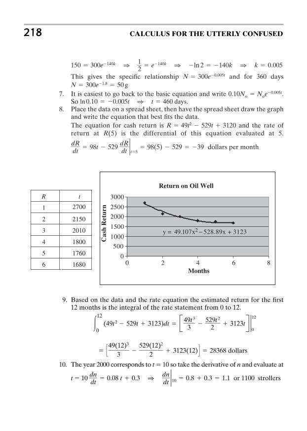
This gives the specific relationship and for 360 days
7. It is easiest to go back to the basic equation and write .So .
8. Place the data on a spread sheet, then have the spread sheet draw the graphand write the equation that best fits the data.The equation for cash return is and the rate ofreturn at R(5) is the differential of this equation evaluated at 5.
dollars per monthdRdt2t5
98(5) 529 39dRdt
98t 529
R 49t2 529t 3120
ln 0.10 0.005t 1 t 460 days0.10No Noe0.005t
N 300e1.8 50 gN 300e0.005t
150 300e140k 1 12 e140k 1 ln 2 140k 1 k 0.005
218 CALCULUS FOR THE UTTERLY CONFUSED
R t
1
2 2150
3 2010
4 1800
5 1760
6 1680
Return on Oil Well
y = 49.107x2 − 528.89x + 3123
0
500
1000
1500
2000
2500
3000
0 2 4 6 8Months
Cas
h R
etu
rn2700
9. Based on the data and the rate equation the estimated return for the first12 months is the integral of the rate statement from 0 to 12.
dollars
10. The year 2000 corresponds to t 10 so take the derivative of n and evaluate at
t 10 dndt
0.08 t 0.3 1 dndt210 0.8 0.3 1.1 or 1100 strollers
S49(12)3
3 529(12)2
2 3123(12)T 28368
312
0(49t 2 529t 3123)dt B49t 3
3 529t 2
2 3123tR 2 12
0
11. Start with the logistic formula and multiply up and down
by so . , the estimated maximum number of
parlors. Substitute to evaluate A.
The logistic formula now reads and substituting
gives the value for k. , ,
, , . The specific formula is f(t)
, and the number of parlors in 1996, is f(6)
12. Take dq/dt and evaluate at 10 months. and
games per month. Depending on where you round off you may
get a number slightly different from this.
dqdt210
70
dqdt
0 5000(2)(0.4)e0.4t
(1 2e0.4t)2
2001 32e1.44 23
t 62001 32e0.24t
k 0.24ln 0.49 3ke3k 0.49
12 32e3k 18812 200
1 32e3kt 3 and f(t) 12
f(t) 200
1 32ekt
6 200
1 A for A 32t 0 and f(t) 6
N 200f(t) N
ekt Ae ktekt
f(t) N
1 Aekt
Exponents and Logarithms 219
220 CALCULUS FOR THE UTTERLY CONFUSED
If our cells aredecaying, why arewe still growing?
Because our growingcells are growingfaster than ourdecaying cells aredecaying.
I knew that.
CHAPTER 10
MORE INTEGRALS
You should read this chapter if you need to review or you need to learn about
Volumes
Arc lengths
Surfaces of revolution
Change of variable
Integration by parts
Partial fractions
Approximation methods
221
Copyright © 2007 by The McGraw-Hill Companies, Inc. Click here for terms of use.
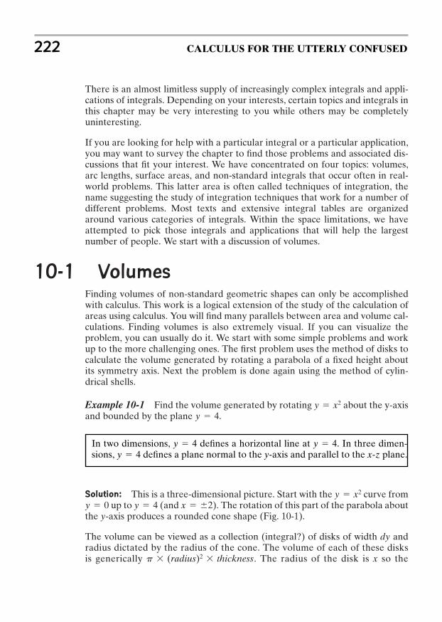
There is an almost limitless supply of increasingly complex integrals and appli-cations of integrals. Depending on your interests, certain topics and integrals inthis chapter may be very interesting to you while others may be completelyuninteresting.
If you are looking for help with a particular integral or a particular application,you may want to survey the chapter to find those problems and associated dis-cussions that fit your interest. We have concentrated on four topics: volumes,arc lengths, surface areas, and non-standard integrals that occur often in real-world problems. This latter area is often called techniques of integration, thename suggesting the study of integration techniques that work for a number ofdifferent problems. Most texts and extensive integral tables are organizedaround various categories of integrals. Within the space limitations, we haveattempted to pick those integrals and applications that will help the largestnumber of people. We start with a discussion of volumes.
10-1 VolumesFinding volumes of non-standard geometric shapes can only be accomplishedwith calculus. This work is a logical extension of the study of the calculation ofareas using calculus. You will find many parallels between area and volume cal-culations. Finding volumes is also extremely visual. If you can visualize theproblem, you can usually do it. We start with some simple problems and workup to the more challenging ones. The first problem uses the method of disks tocalculate the volume generated by rotating a parabola of a fixed height aboutits symmetry axis. Next the problem is done again using the method of cylin-drical shells.
Example 10-1 Find the volume generated by rotating about the y-axisand bounded by the plane .
Solution: This is a three-dimensional picture. Start with the curve fromup to (and ). The rotation of this part of the parabola about
the y-axis produces a rounded cone shape (Fig. 10-1).
The volume can be viewed as a collection (integral?) of disks of width dy andradius dictated by the radius of the cone. The volume of each of these disksis generically . The radius of the disk is x so thep (radius)2 thickness
x 2y 4y 0y x2
y 4y x2
222 CALCULUS FOR THE UTTERLY CONFUSED
In two dimensions, defines a horizontal line at . In three dimen-sions, defines a plane normal to the y-axis and parallel to the x-z plane.y 4
y 4y 4
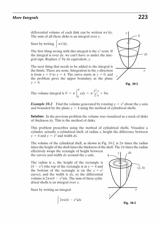
differential volume of each disk can be written .The sum of all these disks is an integral over y.
Start by writing .
The first thing wrong with this integral is the term. Ifthe integral is over dy, we can’t have xs under the inte-gral sign. Replace by its equivalent, y.
The next thing that needs to be added to the integral isthe limits. There are none. Integration in the y-directionis from to . The curve starts at , andthe problem gives the upper boundary as the plane
.
The volume integral is .
Example 10-2 Find the volume generated by rotating about the y-axisand bounded by the plane using the method of cylindrical shells.
Solution: In the previous problem the volume was visualized as a stack of disksof thickness dy. This is the method of disks.
This problem prescribes using the method of cylindrical shells. Visualize acylinder, actually a cylindrical shell, of radius x, height the difference between
and and width dx.
The volume of the cylindrical shell, as shown in Fig. 10-2, is 2 times the radiustimes the height of the shell times the thickness of the shell. The 2 times the radiuseffectively wraps the rectangle of height betweenthe curves and width dx around the y-axis.
The radius is x, the height of the rectangle is(the top of the rectangle is at and
the bottom of the rectangle is on the curve), and the width is dx, so the differentialvolume is . The sum of these cylin-drical shells is an integral over x.
Start by writing an integral
3 2px(4 x2)dx
2px(4 x2)dx
y x2y 4(4 x2)
p
p
y x2y 4
y 4y x2
V p 34
0ydy p
y2
2 P4
0 8p
y 4
y 0y 4y 0
x2
x2
3px2dy
px2dy
More Integrals 223
Fig. 10-2
Fig. 10-1
4
z
y
x
dx
(2, 4)
4
4
z
y
x
dy
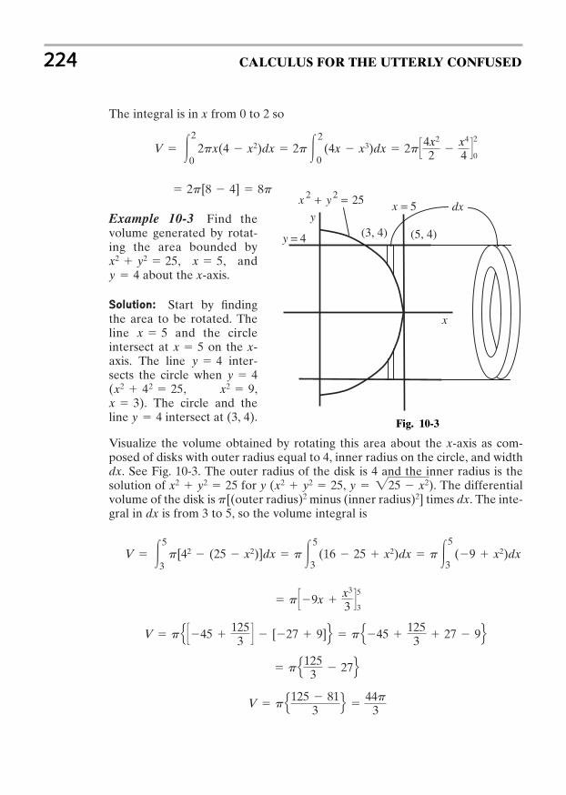
The integral is in x from 0 to 2 so
Example 10-3 Find thevolume generated by rotat-ing the area bounded by
, , andabout the x-axis.
Solution: Start by findingthe area to be rotated. Theline and the circleintersect at on the x-axis. The line inter-sects the circle when ( , ,
). The circle and theline intersect at (3, 4).
Visualize the volume obtained by rotating this area about the x-axis as com-posed of disks with outer radius equal to 4, inner radius on the circle, and widthdx. See Fig. 10-3. The outer radius of the disk is 4 and the inner radius is thesolution of for y ( , ). The differentialvolume of the disk is [(outer radius)2 minus (inner radius)2] times dx. The inte-gral in dx is from 3 to 5, so the volume integral is
V pU125 81
3 V 44p
3
pU125
3 27V
V pU S45 125
3 T [27 9]V pU45 1253 27 9V
p S9x x3
3 T5
3
V 35
3p[42 (25 x2)]dx p 3
5
3(16 25 x2)dx p 3
5
3(9 x2)dx
p
y 225 x2x2 y2 25x2 y2 25
y 4x 3
x2 9x2 42 25y 4
y 4x 5
x 5
y 4x 5x2 y2 25
2p[8 4] 8p
V 32
02px(4 x2)dx 2p 3
2
0(4x x3)dx 2p S4x2
2 x4
4 T2
0
224 CALCULUS FOR THE UTTERLY CONFUSED
Fig. 10-3
x
y
(5, 4)(3, 4)
2522 =+ yx 5=x
4=y
dx
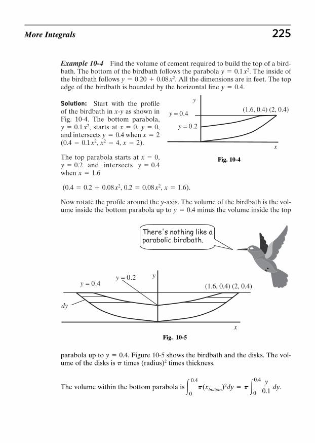
Example 10-4 Find the volume of cement required to build the top of a bird-bath. The bottom of the birdbath follows the parabola . The inside ofthe birdbath follows . All the dimensions are in feet. The topedge of the birdbath is bounded by the horizontal line .
Solution: Start with the profileof the birdbath in x-y as shown inFig. 10-4. The bottom parabola,
, starts at , ,and intersects when ( , , ).
The top parabola starts at ,and intersects
when
( , , ).
Now rotate the profile around the y-axis. The volume of the birdbath is the vol-ume inside the bottom parabola up to minus the volume inside the topy 0.4
x 1.60.2 0.08 x20.4 0.2 0.08 x2
x 1.6y 0.4y 0.2x 0
x 2x2 40.4 0.1 x2x 2y 0.4y 0x 0y 0.1 x2
y 0.4y 0.20 0.08 x2
y 0.1 x2
More Integrals 225
Fig. 10-4
Fig. 10-5
parabola up to . Figure 10-5 shows the birdbath and the disks. The vol-ume of the disks is times (radius)2 times thickness.
The volume within the bottom parabola is .30.4
0p(xbottom)2dy p 3
0.4
0
y0.1
dy
p
y 0.4
(1.6, 0.4) (2, 0.4)
2.0=y
y
x
4.0=y
(1.6, 0.4) (2, 0.4)
y
x
4.0=y
dy
2.0=y
There's nothing like a parabolic birdbath.
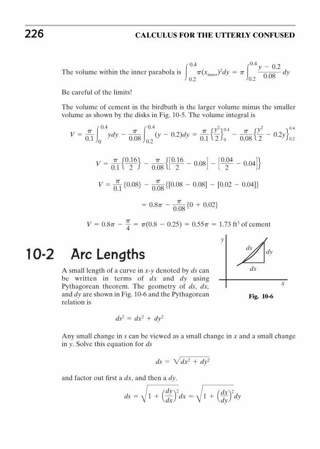
The volume within the inner parabola is
Be careful of the limits!
The volume of cement in the birdbath is the larger volume minus the smallervolume as shown by the disks in Fig. 10-5. The volume integral is
10-2 Arc LengthsA small length of a curve in x-y denoted by ds canbe written in terms of dx and dy usingPythagorean theorem. The geometry of ds, dx,and dy are shown in Fig. 10-6 and the Pythagoreanrelation is
Any small change in s can be viewed as a small change in x and a small changein y. Solve this equation for ds
and factor out first a dx, and then a dy.
ds Å
1 QdydxR
2dx
Å1 Q
dxdyR
2dy
ds 2dx2 dy2
ds2 dx2 dy2
V 0.8p p4 p(0.8 0.25) 0.55p 1.73 ft3 of cement
0.8p p
0.08 50 0.026
V p
0.150.086
p0.08 5[0.08 0.08] [0.02 0.04]6
V p
0.1U
0.162 V
p0.08 U S
0.162 0.08T S
0.042 0.04T V
V p
0.1 30.4
0ydy
p0.08 3
0.4
0.2(y 0.2)dy
p
0.1U
y2
2 V0.4
0p
0.08 Uy2
2 0.2yV0.4
0.2
30.4
0.2p(xinner)
2dy p 30.4
0.2
y 0.20.08 dy
226 CALCULUS FOR THE UTTERLY CONFUSED
dy
dx
dsy
x
Fig. 10-6
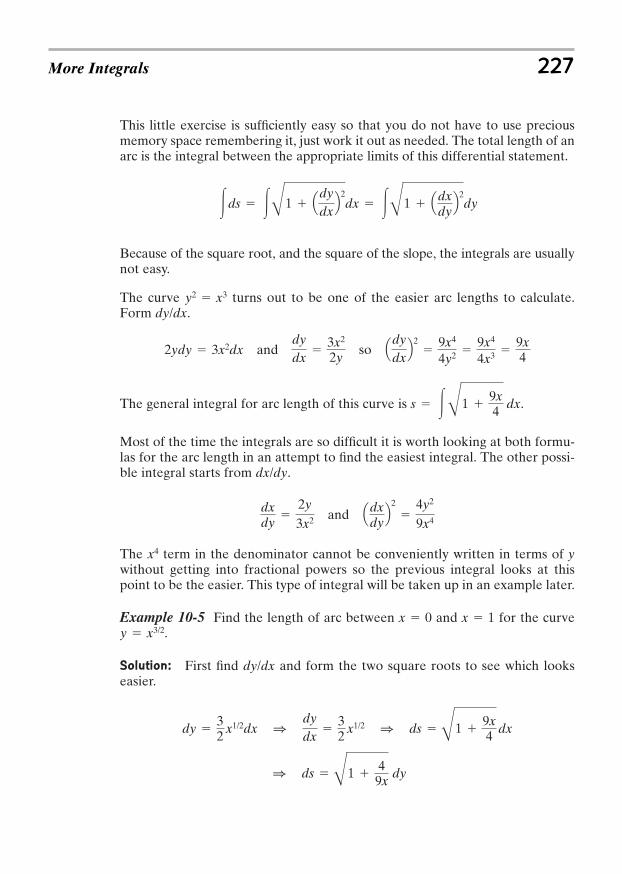
This little exercise is sufficiently easy so that you do not have to use preciousmemory space remembering it, just work it out as needed. The total length of anarc is the integral between the appropriate limits of this differential statement.
Because of the square root, and the square of the slope, the integrals are usuallynot easy.
The curve turns out to be one of the easier arc lengths to calculate.Form .
and so
The general integral for arc length of this curve is .
Most of the time the integrals are so difficult it is worth looking at both formu-las for the arc length in an attempt to find the easiest integral. The other possi-ble integral starts from .
and
The term in the denominator cannot be conveniently written in terms of ywithout getting into fractional powers so the previous integral looks at thispoint to be the easier. This type of integral will be taken up in an example later.
Example 10-5 Find the length of arc between x 0 and x 1 for the curve.
Solution: First find dy/dx and form the two square roots to see which lookseasier.
1 ds Å
1 49x
dy
dy 32 x1/2dx 1
dydx
32 x1/2 1 ds
Å1
9x4 dx
y x3/2
x4
QdxdyR
2
4y2
9x4dxdy
2y
3x2
dx/dy
s 3Å1 9x4 dx
QdydxR
2
9x4
4y2 9x4
4x3 9x4
dydx
3x2
2y2ydy 3x2dx
dy/dxy2 x3
3ds 3Å1 QdydxR
2dx 3Å1 Q
dxdyR
2dy
More Integrals 227
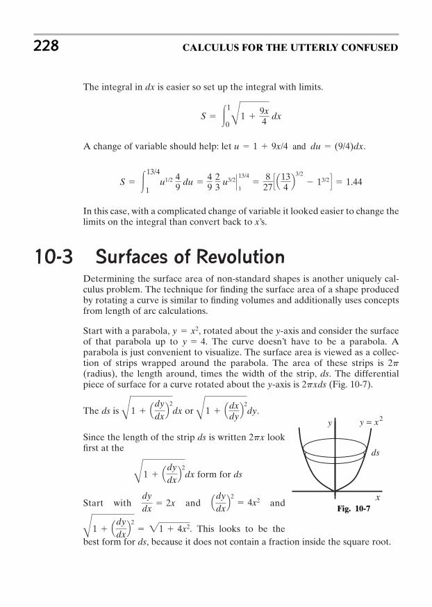
The integral in dx is easier so set up the integral with limits.
A change of variable should help: let .
In this case, with a complicated change of variable it looked easier to change thelimits on the integral than convert back to x’s.
10-3 Surfaces of RevolutionDetermining the surface area of non-standard shapes is another uniquely cal-culus problem. The technique for finding the surface area of a shape producedby rotating a curve is similar to finding volumes and additionally uses conceptsfrom length of arc calculations.
Start with a parabola, , rotated about the y-axis and consider the surfaceof that parabola up to . The curve doesn’t have to be a parabola. Aparabola is just convenient to visualize. The surface area is viewed as a collec-tion of strips wrapped around the parabola. The area of these strips is 2p(radius), the length around, times the width of the strip, ds. The differentialpiece of surface for a curve rotated about the y-axis is (Fig. 10-7).
The ds is or .
Since the length of the strip ds is written lookfirst at the
form for ds
Start with and and
. This looks to be thebest form for ds, because it does not contain a fraction inside the square root.Å
1 QdydxR
2 21 4x2
QdydxR
2 4x2
dydx
2x
Å1 Q
dydxR
2dx
2px
Å1 Q
dxdyR
2dy
Å1 Q
dydxR
2dx
2pxds
y 4y x2
S 313/4
1u1/2 4
9 du 49
23 u3/2 P
13/4
1
827 S Q
134 R
3/2
13/2T 1.44
u 1 9x/4 and du (9/4)dx
S 31
0Å1
9x4 dx
228 CALCULUS FOR THE UTTERLY CONFUSED
ds
y
x
2xy =
Fig. 10-7
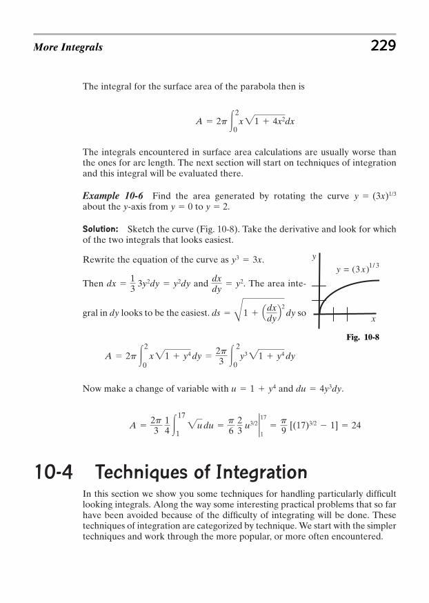
The integral for the surface area of the parabola then is
The integrals encountered in surface area calculations are usually worse thanthe ones for arc length. The next section will start on techniques of integrationand this integral will be evaluated there.
Example 10-6 Find the area generated by rotating the curve about the y-axis from y 0 to y 2.
Solution: Sketch the curve (Fig. 10-8). Take the derivative and look for whichof the two integrals that looks easiest.
Rewrite the equation of the curve as .
Then and . The area inte-
gral in dy looks to be the easiest. so
Now make a change of variable with and .
10-4 Techniques of IntegrationIn this section we show you some techniques for handling particularly difficultlooking integrals. Along the way some interesting practical problems that so farhave been avoided because of the difficulty of integrating will be done. Thesetechniques of integration are categorized by technique. We start with the simplertechniques and work through the more popular, or more often encountered.
A 2p3
14 3
17
12u du
p
623 u3/2 2 17
1p9 [(17)3/2 1] 24
du 4y3dyu 1 y4
A 2p 32
0x21 y4 dy
2p3 3
2
0y321 y4 dy
ds Å
1 QdxdyR
2dy
dxdy
y2dx 13 3y2dy y2dy
y3 3x
y (3x)1/3
A 2p 32
0x21 4x2dx
More Integrals 229
x
y3/1)3( xy =
Fig. 10-8
Change of Variable
The change of variable technique is also called the method of substitution. Asthe names imply the approach is to define a new variable that will transform theintegral to one that is a standard form. The procedure is to define a new vari-able, take the derivative of that new variable and then write the integral interms of the new variable and derivative. There is some skill in picking the newvariable and sometimes you just have to try a few. The best first guess for achange of variable is to look for the worst looking part of the integral and makethat worst looking part the new variable or at least incorporate it into the newvariable. The best way to understand any of these techniques is to jump right inand start doing some problems.
Example 10-7 Find .
Solution: Make a change of variable. Let so that . Thistransforms the integral.
Remember to translate back to the original variable at the end of the problem.
Example 10-8 Find .
Solution: The worst looking part of this integral is the lnx so make a substitu-
tion v ln x so that . This transforms the integral into a standard form.
This is a bit of a strange answer, but then it was a bit of a strange integral.
Example 10-9 Find .
Solution: A new variable would allow the to be written as apower, and integrals of a variable raised to a power d (variable) are standard inte-grals. Let with . The integral is transformed and solved.
3 23 2xdx 12 3w1/2dw
12
w3/2
3/2
13 w 3/2
13 (3 2x)3/2
dw 2dxw 3 2x
23 2x3 2x
123 2xdx
3 dxx lnx
3 1v dv lnv ln(lnx)
dv 1x dx
3 dxx lnx
3 xex 2dx 12 3 eudu
12 eu
12 e x 2
du 2xdxu x2
3 xe x 2dx
230 CALCULUS FOR THE UTTERLY CONFUSED
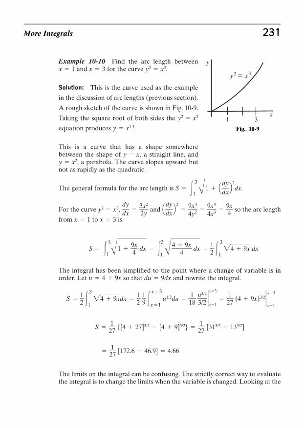
Example 10-10 Find the arc length betweenand for the curve .
Solution: This is the curve used as the example
in the discussion of arc lengths (previous section).
A rough sketch of the curve is shown in Fig. 10-9.
Taking the square root of both sides the
equation produces .
This is a curve that has a shape somewherebetween the shape of , a straight line, and
, a parabola. The curve slopes upward butnot as rapidly as the quadratic.
The general formula for the arc length is .
For the curve , and so the arc length
from to is
The integral has been simplified to the point where a change of variable is inorder. Let so that and rewrite the integral.
The limits on the integral can be confusing. The strictly correct way to evaluatethe integral is to change the limits when the variable is changed. Looking at the
127 [172.6 46.9] 4.66
S 127 5[4 27]3/2 [4 9]3/26
127 [313/2 133/2]
S 12 3
3
124 9xdx
12
19 3
x3
x1u1/2du
118
u3/2
3/22 x3
x1
127 (4 9x)3/2 2 x3
x1
du 9dxu 4 9x
S 33
1 Å1
9x4 dx 3
3
1 Å4 9x
4 dx 12 3
3
124 9x dx
x 3x 1
QdydxR
2
9x4
4y2 9x4
4x3 9x4
dydx
3x2
2yy2 x3
S 33
1 Å1 Q
dydxR
2dx
y x2y x
y x1.5
y2 x3
y2 x3x 3x 1
More Integrals 231
31
32 xy =
x
y
Fig. 10-9
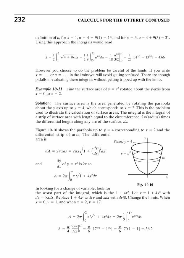
definition of u; for , , and for , u 4 9(3) 31.Using this approach the integrals would read
However you choose to do the problem be careful of the limits. If you writeor in the limits you will avoid getting confused. There are enough
pitfalls in evaluating these integrals without getting tripped up with the limits.
Example 10-11 Find the surface area of rotated about the y-axis fromto .
Solution: The surface area is the area generated by rotating the parabolaabout the y-axis up to , which corresponds to . This is the problemused to illustrate the calculation of surface areas. The integral is the integral ofa strip of surface area with length equal to the circumference, (radius) timesthe differential length along any arc of the surface, ds.
Figure 10-10 shows the parabola up to corresponding to and thedifferential strip of area. The differentialarea is
and of is so
In looking for a change of variable, look forthe worst part of the integral, which is the . Let with
. Replace with v and with . Change the limits. When, , and when , .
A p4 S
v3/2
3/2T17
1p
6 [173/2 13/2]
p
6 [70.1 1] 36.2
A 2p 32
0x21 4x2dx 2p 1
8 317
1v1//2dv
v 17x 2v 1x 0dv/8xdx1 4x2dv 8xdx
v 1 4x21 4x2
A 2p 32
0x21 4x2dx
2xy x2dydx
dA 2pxds 2pxÅ
1 QdydxR
2dx
x 2y 4
2p
x 2y 4
x 2x 0y x2
u cx c
S 12 3
3
124 9xdx
12
19 3
31
13u1/2du
118
u3/2
3/22 31
13
127
[313/2 133/2] 4.66
x 3u 4 9(1) 13x 1
232 CALCULUS FOR THE UTTERLY CONFUSED
4=y
2xy =ds
yPlane,
x
Fig. 10-10

Example 10-12 Find .
Solution: The worst part of this integral is the so let and. The integral transforms to a standard integral.
Example 10-13 The price of a product varies with supply and demand in sucha way that with k to be determined by conditions. Find theprice as a function of time and graph the price vs. time. The price is $4.50 when
, and $4.00 when . The t is in years.
Solution: The first step in solving for is to write the rate statement in aform that can be integrated.
or
Deal with this integral in p as a separate exercise. Make a substitution forby letting so and the integral becomes
With this little side calculation and remembering that integrating
produces a constant of integration, the integration produces
Rearranging for convenience in writing as an exponent: ln(5 2p) 2kt 2C. And writing as an exponential (This is the only way to get an equation thatreads ) we get
The constant of integration can be carried as long as you like but defining a newconstant at this point looks convenient. Make equal to 2D.
p 2.5 De2kt
2p 5 2De2kt
e2C
5 2p e2kt2C e2kte2C
p . . .
12 ln (5 2p) kt C
3 dp5 2p
3kdt
3 dp5 2p
12 3
dzz
12 lnz
12 ln(5 2p)
dz 2dpz 5 2p5 2p
3 dp5 2p
3 kdtdp
5 2p kdt
p(t)
t 2t 0
dp/dt k(5 2p)
3 tan (3x 2)dx 13 3 tan wdw
13 ln (cos w)
13 ln [ cos (3x 2)]
dw 3dxw 3x 23x 2
3 tan (3x 2)dx
More Integrals 233
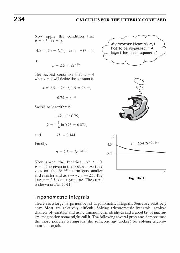
Now apply the condition thatat .
and
so
The second condition that when will define the constant k.
, ,
Switch to logarithms:
,
,
and
Finally,
Now graph the function. At ,as given in the problem. As time
goes on, the term gets smallerand smaller and as , . Theline is an asymptote. The curveis shown in Fig. 10-11.
Trigonometric Integrals
There are a large, large number of trigonometric integrals. Some are relativelyeasy. Most are relatively difficult. Solving trigonometric integrals involveschanges of variables and using trigonometric identities and a good bit of ingenu-ity, imagination some might call it. The following several problems demonstratethe more popular techniques (did someone say tricks?) for solving trigono-metric integrals.
p 2.5p S 2.5t S `
2e0.144tp 4.5
t 0
p 2.5 2e0.144t
2k 0.144
k 14 ln 0.75 0.072
4k ln 0.75
0.75 e4k
1.5 2e4k4 2.5 2e4k
t 2p 4
p 2.5 2e2kt
D 24.5 2.5 D(1)
t 0p 4.5
234 CALCULUS FOR THE UTTERLY CONFUSED
My brother Newt always has to be reminded, " Alogarithm is an exponent."
ep 25.2 +=
2.5
4.5
t
p
−0.144t
Fig. 10-11
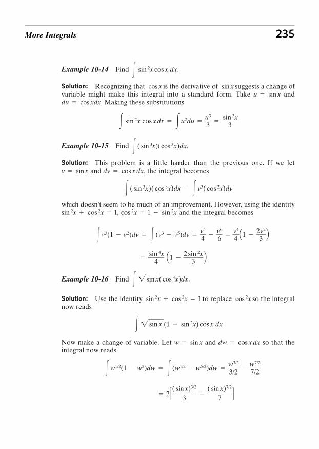
Example 10-14 Find .
Solution: Recognizing that is the derivative of suggests a change ofvariable might make this integral into a standard form. Take and
. Making these substitutions
Example 10-15 Find .
Solution: This problem is a little harder than the previous one. If we letand , the integral becomes
which doesn’t seem to be much of an improvement. However, using the identity, and the integral becomes
Example 10-16 Find .
Solution: Use the identity to replace so the integralnow reads
Now make a change of variable. Let and so that theintegral now reads
2 S( sin x)3/2
3 ( sin x)7/2
7 T
3w1/2(1 w2)dw 3 (w1/2 w5/2)dw w3/2
3/2
w7/2
7/2
dw cos x dxw sin x
3 2 sin x (1 sin 2x) cos x dx
cos 2xsin 2x cos 2x 1
3 2 sin x( cos 3x)dx
sin 4x
4 Q1 2 sin 2x
3 R
3 v3(1 v2)dv 3 (v3 v5)dv v4
4 v6
6
v4
4 Q1 2v2
3 R
cos 2x 1 sin 2xsin 2x cos 2x 1
3 ( sin 3x)( cos 3x)dx 3 v3( cos 2x)dv
dv cos x dxv sin x
3 ( sin 3x)( cos 3x)dx
3 sin 2x cos x dx 3 u2du u3
3 sin 3x
3
du cos xdxu sin x
sin xcos x
3 sin 2x cos x dx
More Integrals 235
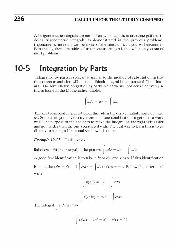
All trigonometric integrals are not this easy. Though there are some patterns todoing trigonometric integrals, as demonstrated in the previous problems,trigonometric integrals can be some of the most difficult you will encounter.Fortunately, there are tables of trigonometric integrals that will help you out ofmost problems.
10-5 Integration by PartsIntegration by parts is somewhat similar to the method of substitution in that
the correct association will make a difficult integral into a not so difficult inte-gral. The formula for integration by parts, which we will not derive or even jus-tify, is found in the Mathematical Tables.
The key to successful application of this rule is the correct initial choice of u anddv. Sometimes you have to try more than one combination to get one to workwell. The purpose of the choice is to make the integral on the right side easierand not harder than the one you started with. The best way to learn this is to godirectly to some problems and see how it is done.
Example 10-17 Find .
Solution: Fit the integral to the pattern .
A good first identification is to take as dv, and x as u. If this identification
is made then and makes . Follow the pattern and
write
The integral is so
3 xexdx xex ex ex(x 1)
ex3 exdx
3 x(exdx) xex 3 exdx
3 u(dv) uv 3 vdu
ex v3 exdx 3 dvdu dx
exdx
3 udv uv 3 vdu
3 xexdx
3 udv uv 3 vdu
236 CALCULUS FOR THE UTTERLY CONFUSED
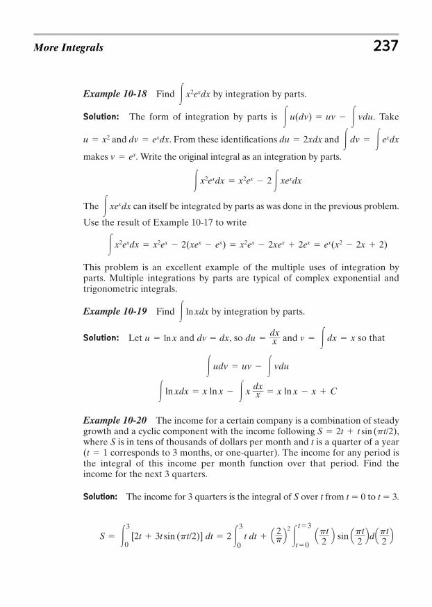
Example 10-18 Find by integration by parts.
Solution: The form of integration by parts is . Take
and . From these identifications and
makes . Write the original integral as an integration by parts.
The can itself be integrated by parts as was done in the previous problem.
Use the result of Example 10-17 to write
This problem is an excellent example of the multiple uses of integration byparts. Multiple integrations by parts are typical of complex exponential andtrigonometric integrals.
Example 10-19 Find by integration by parts.
Solution: Let and dv dx, so and so that
Example 10-20 The income for a certain company is a combination of steadygrowth and a cyclic component with the income following ,where S is in tens of thousands of dollars per month and t is a quarter of a year( corresponds to 3 months, or one-quarter). The income for any period isthe integral of this income per month function over that period. Find theincome for the next 3 quarters.
Solution: The income for 3 quarters is the integral of S over t from t 0 to t 3.
S 33
0[2t 3t sin (pt/2)] dt 2 3
3
0t dt Q
2pR
2
3t3
t0Qpt2 R sin Qpt
2 RdQpt2 R
t 1
S 2t t sin (pt/2)
3 ln xdx x ln x 3 x dxx x ln x x C
3 udv uv 3 vdu
v 3 dx xdu dxxu ln x
3 ln xdx
3 x2exdx x2ex 2(xex ex) x2ex 2xex 2ex ex(x2 2x 2)
3 xexdx
3 x2exdx x2ex 2 3 xexdx
v ex
3 dv 3 exdxdu 2xdxdv exdxu x2
3 u(dv) uv 3 vdu
3 x2exdx
More Integrals 237
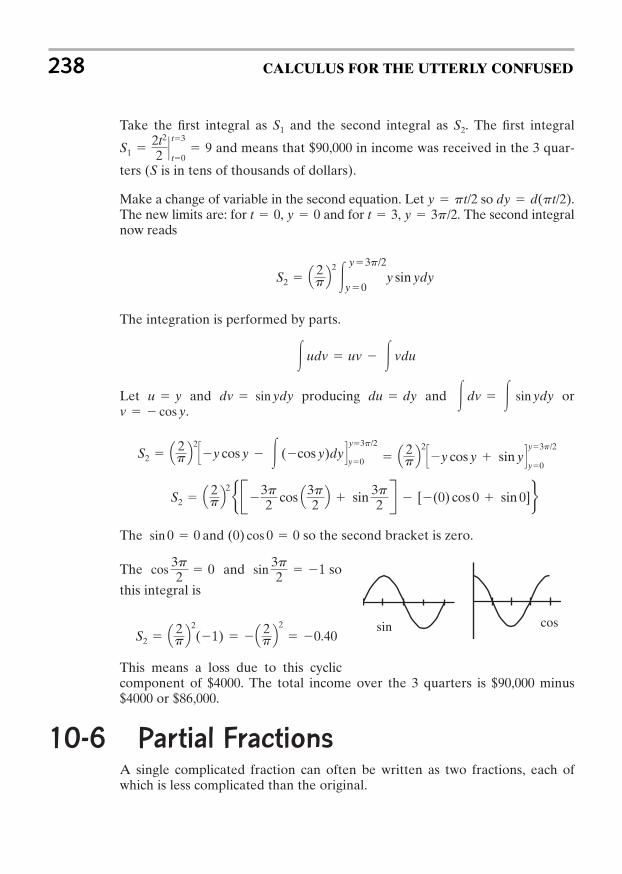
Take the first integral as and the second integral as . The first integral
and means that $90,000 in income was received in the 3 quar-
ters (S is in tens of thousands of dollars).
Make a change of variable in the second equation. Let so .The new limits are: for , and for , . The second integralnow reads
The integration is performed by parts.
Let and producing and or.
The and so the second bracket is zero.
The and so
this integral is
This means a loss due to this cycliccomponent of $4000. The total income over the 3 quarters is $90,000 minus$4000 or $86,000.
10-6 Partial FractionsA single complicated fraction can often be written as two fractions, each ofwhich is less complicated than the original.
S2 Q2pR
2(1) Q
2pR
2
0.40
sin3p2 1cos
3p2 0
(0) cos 0 0sin 0 0
S2 Q2pR
2 b B3p2 cos Q3p2 R sin 3p
2 R [(0) cos 0 sin 0]r
S2 Q2pR
2Sy cos y 3 (cos y)dyT
y3p/2
y0 Q2pR
2Sy cos y sin yT
y3p/2
y0
v cos y3 dv 3 sin ydydu dydv sin ydyu y
3 udv uv 3 vdu
S2 Q2pR
2
3y3p/2
y0y sin ydy
y 3p/2t 3y 0t 0dy d(pt/2)y pt/2
S1 2t2
2 Pt3
t0 9
S2S1
238 CALCULUS FOR THE UTTERLY CONFUSED
sin cos
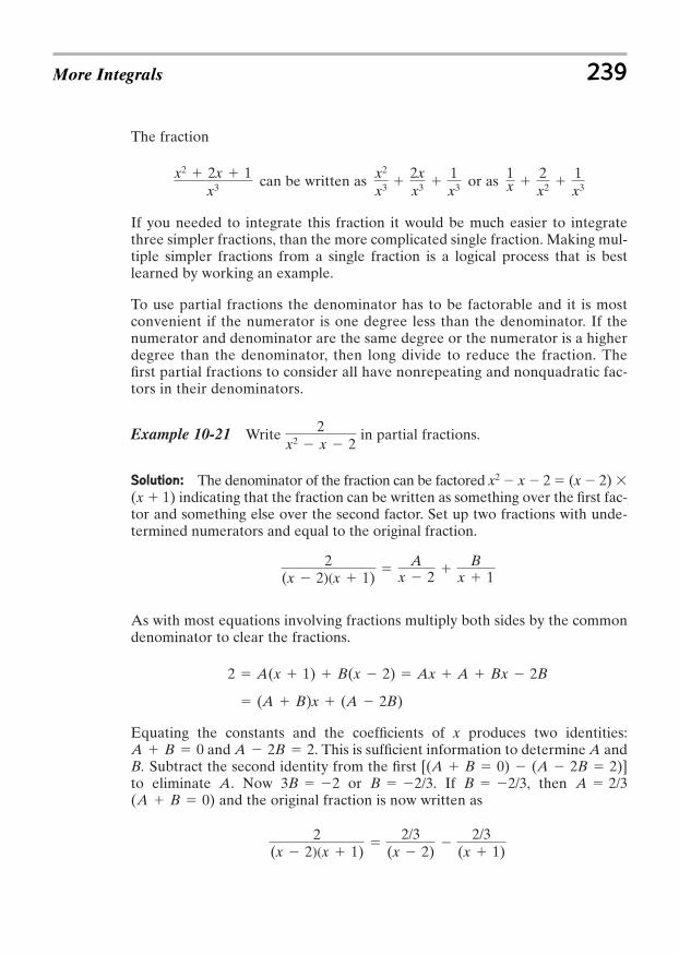
The fraction
can be written as or as
If you needed to integrate this fraction it would be much easier to integratethree simpler fractions, than the more complicated single fraction. Making mul-tiple simpler fractions from a single fraction is a logical process that is bestlearned by working an example.
To use partial fractions the denominator has to be factorable and it is mostconvenient if the numerator is one degree less than the denominator. If thenumerator and denominator are the same degree or the numerator is a higherdegree than the denominator, then long divide to reduce the fraction. Thefirst partial fractions to consider all have nonrepeating and nonquadratic fac-tors in their denominators.
Example 10-21 Write in partial fractions.
Solution: The denominator of the fraction can be factored x2 x 2 (x 2) (x 1) indicating that the fraction can be written as something over the first fac-tor and something else over the second factor. Set up two fractions with unde-termined numerators and equal to the original fraction.
As with most equations involving fractions multiply both sides by the commondenominator to clear the fractions.
Equating the constants and the coefficients of x produces two identities:and . This is sufficient information to determine A and
B. Subtract the second identity from the first [ ]to eliminate A. Now or . If , then ( ) and the original fraction is now written as
2(x 2)(x 1)
2/3
(x 2)
2/3(x 1)
A B 0A 2/3B 2/3B 2/33B 2
(A B 0) (A 2B 2)A 2B 2A B 0
(A B)x (A 2B)
2 A(x 1) B(x 2) Ax A Bx 2B
2(x 2)(x 1)
A
x 2 B
x 1
2x2 x 2
1x
2x2
1x3
x2
x3 2xx3
1x3
x2 2x 1x3
More Integrals 239
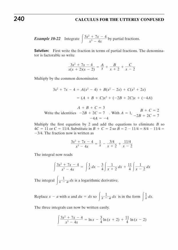
Example 10-22 Integrate by partial fractions.
Solution: First write the fraction in terms of partial fractions. The denomina-tor is factorable so write
Multiply by the common denominator.
Write the identities . With ,
Multiply the first equation by 2 and add the equations to eliminate B soor . Substitute in so B 2 11/4 8/4 11/4
3/4. The fraction now is written as
The integral now reads
The integral is a logarithmic derivative.
Replace with u and so is in the form .
The three integrals can now be written easily.
3 3x2 7x 4x3 4x
ln x 34 ln (x 2)
114 ln (x 2)
3 1x dx3 1
x a dxdu dxx a
3 1x a dx
3 3x2 7x 4x3 4x
3 1x dx
34 3 1
x 2 dx 114 3 1
x 2 dx
3x2 7x 4x3 4x
1x
3/4x 2
11/4x 2
B C 2C 11/44C 11
B C 22B 2C 7
A 1A B C 32B 2C 7
4A 4
(A B C)x2 (2B 2C)x (4A)
3x2 7x 4 A(x2 4) B(x2 2x) C(x2 2x)
3x2 7x 4x(x 2)(x 2)
Ax
Bx 2
Cx 2
3 3x2 7x 4x3 4x
240 CALCULUS FOR THE UTTERLY CONFUSED
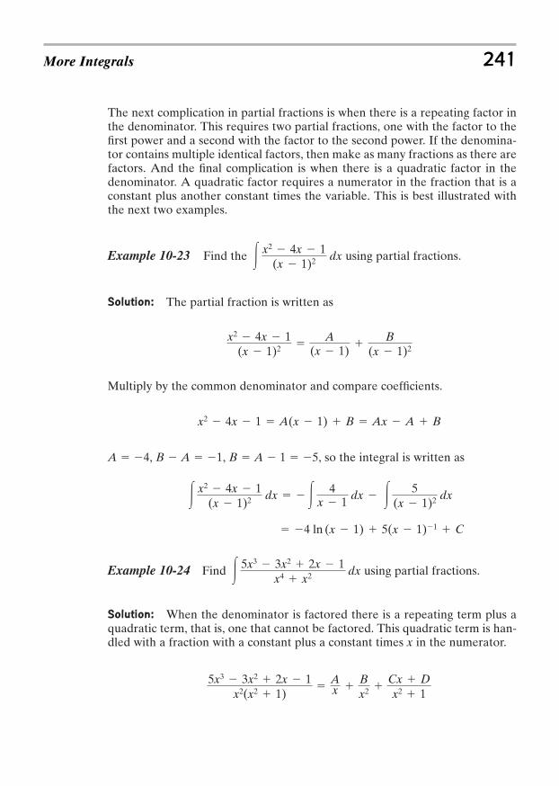
The next complication in partial fractions is when there is a repeating factor inthe denominator. This requires two partial fractions, one with the factor to thefirst power and a second with the factor to the second power. If the denomina-tor contains multiple identical factors, then make as many fractions as there arefactors. And the final complication is when there is a quadratic factor in thedenominator. A quadratic factor requires a numerator in the fraction that is aconstant plus another constant times the variable. This is best illustrated withthe next two examples.
Example 10-23 Find the using partial fractions.
Solution: The partial fraction is written as
Multiply by the common denominator and compare coefficients.
A 4, B A 1, B A 1 5, so the integral is written as
Example 10-24 Find using partial fractions.
Solution: When the denominator is factored there is a repeating term plus aquadratic term, that is, one that cannot be factored. This quadratic term is han-dled with a fraction with a constant plus a constant times x in the numerator.
5x3 3x2 2x 1x2(x2 1)
Ax
Bx2
Cx Dx2 1
3 5x3 3x2 2x 1x4 x2 dx
4 ln (x 1) 5(x 1)1 C
3 x2 4x 1(x 1)2 dx 3 4
x 1dx 3 5
(x 1)2 dx
x2 4x 1 A(x 1) B Ax A B
x2 4x 1(x 1)2
A(x 1)
B
(x 1)2
3 x2 4x 1(x 1)2 dx
More Integrals 241

Multiply by the common denominator and compare coefficients.
so the integral is written as
That last integral came from a Table of Integrals. Quadratic partial fractionsusually produce very difficult integrals.
10-7 Integrals from TablesOne of the best techniques of integration is to use the table of integrals foundin most texts. A table of integrals is found in the Mathematical Tables includedat the back of this book.
Some instructors do not allow the useof tables on tests. We do not sharethat view. Why take up preciousmemory space with formulas that areavailable in an inexpensive mathe-matical table? Regardless of yourinstructor, you will eventually want touse tables, and these examples willgive you an introduction to theprocess. Most tables are organized bycategories: trigonometric, logarith-mic, exponential, quadratics or frac-tions, or whatever. The examples wehave chosen are, hopefully, appropri-ate for what you will encounter.
2 ln u x u x1 32 ln (x2 1) 2 tan 1x K3 5x3 3x2 2x 1
x4 x2 dx
3 5x3 3x2 2x 1x4 x2 dx 2 3 dx
x 3 dxx2 3 3x 2
x2 1dx
B 1, D 2, A 2 and C 3
5x3 3x2 2x 1 (A C)x3 (B D)x2 Ax B
5x3 3x2 2x 1 Ax(x2 1) B(x2 1) (Cx D)x2
242 CALCULUS FOR THE UTTERLY CONFUSED
My sister Liebie never
uses tables. She likes
to show off and work all
the integrals.
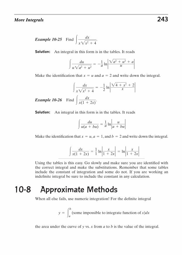
Example 10-25 Find .
Solution: An integral in this form is in the tables. It reads
Make the identification that and and write down the integral.
Example 10-26 Find .
Solution: An integral in this form is in the tables. It reads
Make the identification that , , and and write down the integral.
Using the tables is this easy. Go slowly and make sure you are identified withthe correct integral and make the substitutions. Remember that some tablesinclude the constant of integration and some do not. If you are working anindefinite integral be sure to include the constant in any calculation.
10-8 Approximate MethodsWhen all else fails, use numeric integration! For the definite integral
the area under the curve of y vs. x from a to b is the value of the integral.
y 3b
a(some impossible to integrate function of x)dx
3 dxx(1 2x)
11
ln 2 x1 2x
2 ln 2 x1 2x
2
b 2a 1x u
3 duu(a bu)
1a ln 2 u
a bu2
3 dxx(1 2x)
3 dx
x2x2 4
12 ln 224 x2 2
x 2a 2x u
3 du
u2a2 u2
1a ln 22a2 u2 a
u 2
3 dx
x2x2 4
More Integrals 243
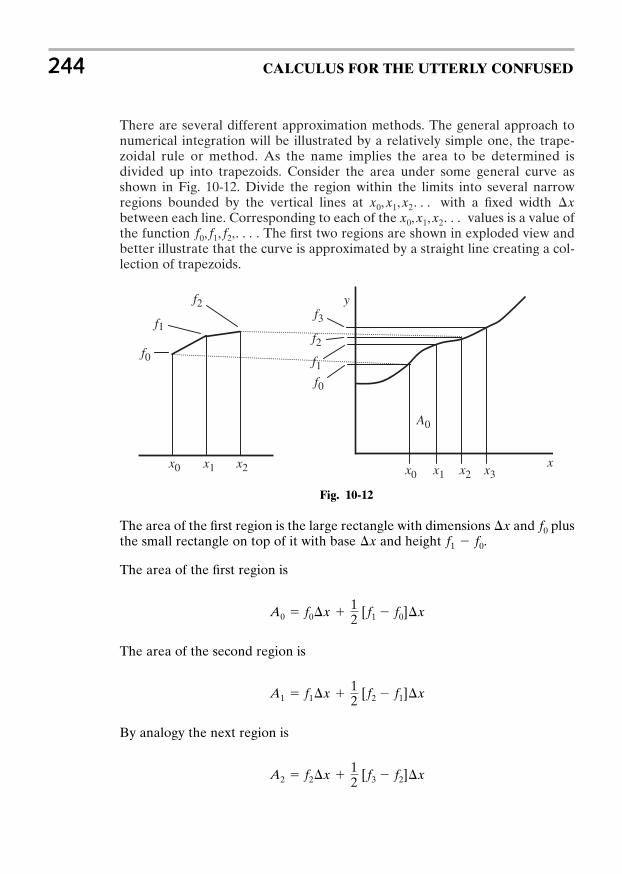
There are several different approximation methods. The general approach tonumerical integration will be illustrated by a relatively simple one, the trape-zoidal rule or method. As the name implies the area to be determined isdivided up into trapezoids. Consider the area under some general curve asshown in Fig. 10-12. Divide the region within the limits into several narrowregions bounded by the vertical lines at with a fixed width between each line. Corresponding to each of the values is a value ofthe function . The first two regions are shown in exploded view andbetter illustrate that the curve is approximated by a straight line creating a col-lection of trapezoids.
f0, f1, f2,cx0, x1, x2c
xx0, x1, x2c
244 CALCULUS FOR THE UTTERLY CONFUSED
Fig. 10-12
The area of the first region is the large rectangle with dimensions and plusthe small rectangle on top of it with base and height .
The area of the first region is
The area of the second region is
By analogy the next region is
A2 f2 x 12 [f3 f2] x
A1 f1 x 12 [f2 f1] x
A0 f0 x 12 [f1 f0] x
f1 f0 xf0 x
A0
f0
f0 f1
f1f2
f2f3
x3x2x2 x1
x1 x0x0
y
x
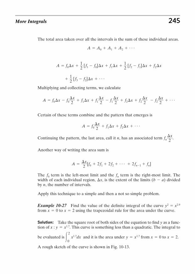
The total area taken over all the intervals is the sum of these individual areas.
Multiplying and collecting terms, we calculate
Certain of these terms combine and the pattern that emerges is
Continuing the pattern, the last area, call it n, has an associated term .
Another way of writing the area sum is
The term is the left-most limit and the term is the right-most limit. Thewidth of each individual region, , is the extent of the limits dividedby n, the number of intervals.
Apply this technique to a simple and then a not so simple problem.
Example 10-27 Find the value of the definite integral of the curve from to using the trapezoidal rule for the area under the curve.
Solution: Take the square root of both sides of the equation to find y as a func-tion of x : . This curve is something less than a quadratic. The integral to
be evaluated is and it is the area under from to .
A rough sketch of the curve is shown in Fig. 10-13.
x 2x 0y x1.732
0x1.7dx
y x1.7
x 2x 0y2 x2.9
(b a) xfnf0
A x2 [f0 2 f1 2 f2 c 2 fn1 fn]
fn x2
A f0 x2 f1 x f2 x c
f2 x2 cA f0 x f0
x2 f1 x f1
x2 f1
x2 f2 x f2
x2
12 [f3 f2] x c
A f0 x 12 [f1 f0] x f1 x
12 [f2 f1] x f2 x
A A0 A1 A2 c
More Integrals 245
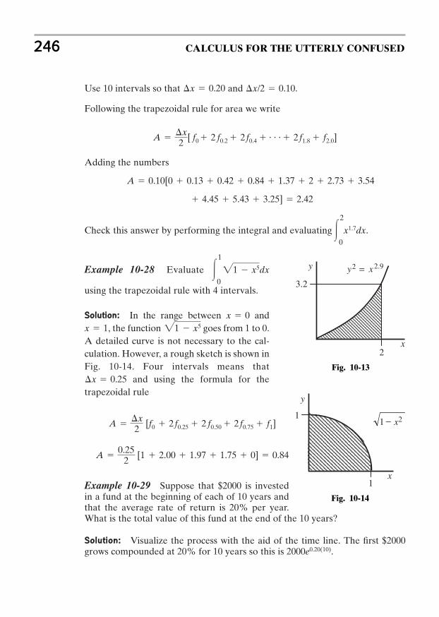
Use 10 intervals so that and .
Following the trapezoidal rule for area we write
Adding the numbers
Check this answer by performing the integral and evaluating .
Example 10-28 Evaluate
using the trapezoidal rule with 4 intervals.
Solution: In the range between and, the function goes from 1 to 0.
A detailed curve is not necessary to the cal-culation. However, a rough sketch is shown inFig. 10-14. Four intervals means that
and using the formula for thetrapezoidal rule
Example 10-29 Suppose that $2000 is investedin a fund at the beginning of each of 10 years andthat the average rate of return is 20% per year.What is the total value of this fund at the end of the 10 years?
Solution: Visualize the process with the aid of the time line. The first $2000grows compounded at 20% for 10 years so this is . 2000e0.20(10)
A 0.25
2 [1 2.00 1.97 1.75 0] 0.84
A x2 [f0 2f0.25 2 f0.50 2 f0.75 f1]
x 0.25
21 x5x 1x 0
31
0
21 x5dx
32
0
x1.7dx
4.45 5.43 3.25] 2.42
A 0.10[0 0.13 0.42 0.84 1.37 2 2.73 3.54
A x2 [ f0 2 f0.2 2 f0.4 c 2 f1.8 f2.0]
x/2 0.10 x 0.20
246 CALCULUS FOR THE UTTERLY CONFUSED
2.92 xy =3.2
2x
y
Fig. 10-13
21 xy =
1
1
y
x
−
Fig. 10-14
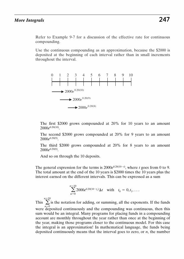
Refer to Example 9-7 for a discussion of the effective rate for continuouscompounding.
Use the continuous compounding as an approximation, because the $2000 isdeposited at the beginning of each interval rather than in small incrementsthroughout the interval.
More Integrals 247
)10(20.02000
0 1 2 3 4 5 6 7 8 9 10
e
)9(20.02000e
)8(20.02000e
The first $2000 grows compounded at 20% for 10 years to an amount.
The second $2000 grows compounded at 20% for 9 years to an amount.
The third $2000 grows compounded at 20% for 8 years to an amount.
And so on through the 10 deposits.
The general expression for the terms is , where t goes from 0 to 9.The total amount at the end of the 10 years is $2000 times the 10 years plus theinterest earned on the different intervals. This can be expressed as a sum
with
This is the notation for adding, or summing, all the exponents. If the funds
were deposited continuously and the compounding was continuous, then thissum would be an integral. Many programs for placing funds in a compoundingaccount are monthly throughout the year rather than once at the beginning ofthe year, making those programs closer to the continuous model. For this casethe integral is an approximation! In mathematical language, the funds beingdeposited continuously means that the interval goes to zero, or n, the number
an10
n0
t0 0, t1, can10
n02000e0.20(10tn) t
2000e0.20(10t)
2000e0.20(8)
2000e0.20(9)
2000e0.20(10)
of intervals, goes to infinity. In symbolic language we write
The exponent can be reworked to so the integral for thetotal amount is
Make a change of variable and integrate.
This number is lower than the actual amount if the funds were deposited at thebeginning of each year. If the funds were placed continuously throughout theyear then this number is correct. Programs for making calculations similar tothis one are usually found in financial calculators. If you have one, check thisanswer with the answer from your calculator. Your calculator uses a calculatingalgorithm similar, if not identical, to the summation notation used earlier in theproblem.
Find volumes by discs and shells
Know the formula for arc length
Wrap the arc length for surfaces of revolution
Integrate by changing variables
Use integration by parts
Apply partial fractions
Know how to use tables
Be able to apply approximation methods
A 10,000e2 [e2 1] 10,000e2 S1 1e2 T $63900
A 2000
0.20 e 2310
0e0.20td(0.20t) 10,000 e 2 Se0.20tT
10
0
A 2000e2 310
0e0.20tdt
e0.20(10t) e2e0.20t
limnS`
an
2000e0.20(10tn) t 310
02000e0.20(10t)dt
248 CALCULUS FOR THE UTTERLY CONFUSED
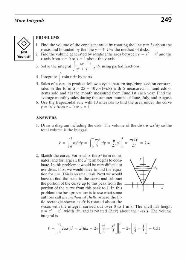
PROBLEMS
1. Find the volume of the cone generated by rotating the line y 3x about they-axis and bounded by the line y 4. Use the method of disks.
2. Find the volume generated by rotating the area between and thex-axis from x 0 to x 1 about the y-axis.
3. Solve the integral using partial fractions.
4. Integrate by parts.
5. Sales of a certain product follow a cyclic pattern superimposed on constantsales in the form with S measured in hundreds ofitems sold and t is the month measured from June 1st each year. Find theaverage monthly sales during the summer months of June, July, and August.
6. Use the trapezoidal rule with 10 intervals to find the area under the curvefrom x = 0 to x 1.
ANSWERS
1. Draw a diagram including the disk. The volume of the disk is so thetotal volume is the integral
2. Sketch the curve. For small x the x2 term domi-nates, and for larger x the x3 term begins to dom-inate. In this problem it would be very difficult touse disks. First we would have to find the equa-tion for x . This is no small task. Next we wouldhave to find the peak in the curve and subtractthe portion of the curve up to this peak from theportion of the curve from this peak to 1. In thisproblem the best procedure is to use what someauthors call the method of shells, where the lit-tle rectangle shown as dx is rotated about they-axis with the integral carried out over 0 to 1 in x. The shell has height
, width dx, and is rotated (2px) about the y-axis. The volumeintegral is
V 31
02px(x2 x3)dx 2pB x4
4 x5
5R 2 1
0
2pB14
15R 0.31
y x2 x3
V 34
0px2dy 3
4
0
py2
9 dy p27 y3 2 4
0p(4)3
27 7.4
px2dy
y 2x
S 25 10 cos (pt/8)
3 x sin x dx
3 4x 1x2 x 2
dx
y x2 x3
More Integrals 249
dy
y
x
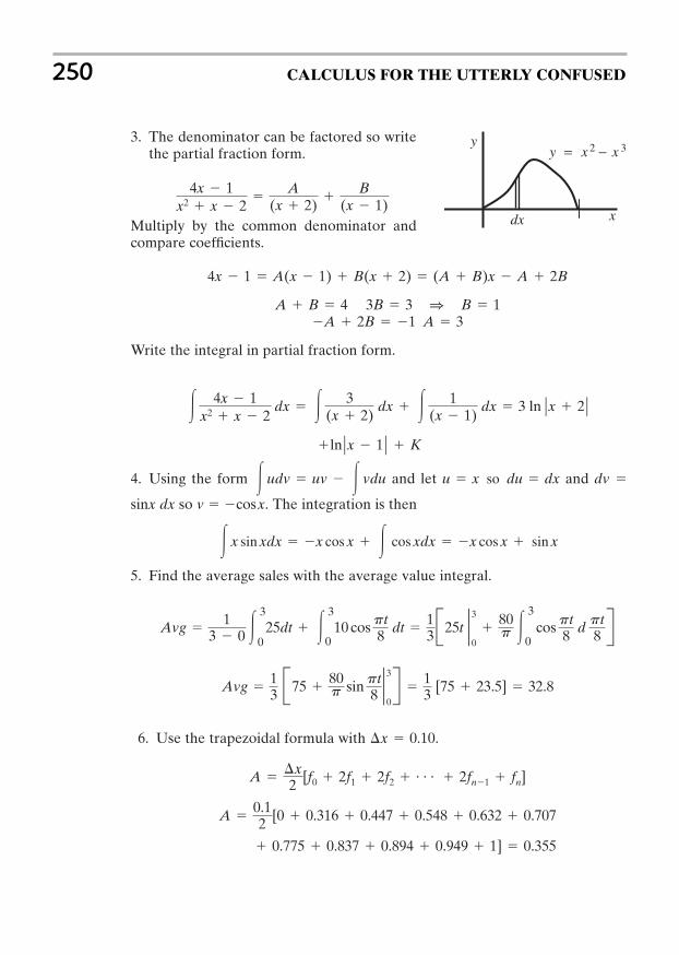
3. The denominator can be factored so writethe partial fraction form.
Multiply by the common denominator andcompare coefficients.
Write the integral in partial fraction form.
4. Using the form and let and dv
sinx dx so v cosx. The integration is then
5. Find the average sales with the average value integral.
6. Use the trapezoidal formula with .
A 0.12 [0 0.316 0.447 0.548 0.632 0.707
0.775 0.837 0.894 0.949 1] 0.355
A x2 [f0 2f1 2f2 c 2fn1 fn]
x 0.10
Avg 13 B75
80p sinpt
82 30
R 13 [75 23.5] 32.8
Avg 1
3 0 33
025dt 3
3
010 cospt
8 dt 13B25t 2 3
0
80p 3
3
0cospt
8 d pt8 R
3 x sin xdx x cos x 3 cos xdx x cos x sin x
u x so du dx3 udv uv 3 vdu
lnZx 1Z K
3 4x 1x2 x 2
dx 3 3(x 2)
dx 3 1(x 1)
dx 3 ln Zx 2Z
A 2B 1 A 3A B 4 3B 3 1 B 1
4x 1 A(x 1) B(x 2) (A B)x A 2B
4x 1x2 x 2
A
(x 2)
B(x 1)
250 CALCULUS FOR THE UTTERLY CONFUSED
32 xxy =
dx
y
x
−

More Integrals 251
Did you enjoy the book?Oh yes, I'm looking forward to the movie!
I'd like to playCaptain Calculus.
I see you more as the bird singing on the natural log.
Liebie, you're an
incurable romantic. I'm smart, too.

This page intentionally left blank

MATHEMATICALTABLES
253
Copyright © 2007 by The McGraw-Hill Companies, Inc. Click here for terms of use.
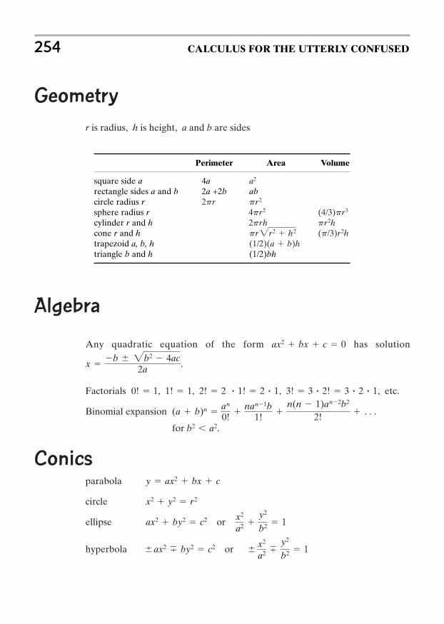
Geometry
r is radius, h is height, a and b are sides
254 CALCULUS FOR THE UTTERLY CONFUSED
Perimeter Area Volume
square side a 4arectangle sides a and b 2a +2b abcircle radius rsphere radius rcylinder r and hcone r and htrapezoid a, b, htriangle b and h (1/2)bh
(1/2)(a b)h(p/3)r2hpr2r2 h2pr2h2prh(4/3)pr34pr2
pr22pr
a2
Algebra
Any quadratic equation of the form has solution
.
Factorials
Binomial expansion
.
Conicsparabola
circle
ellipse or
hyperbola or x2
a2 7y2
b2 1 ax2 7 by2 c2
x2
a2 y2
b2 1ax2 by2 c2
x2 y2 r2
y ax2 bx c
for b2 a2
(a b)n an
0!
nan1b1!
n(n 1)an2b2
2! c
0! 1, 1! 1, 2! 2 ? 1! 2 ? 1, 3! 3 ? 2! 3 ? 2 ? 1, etc.
x b 2b2 4ac
2a
ax2 bx c 0
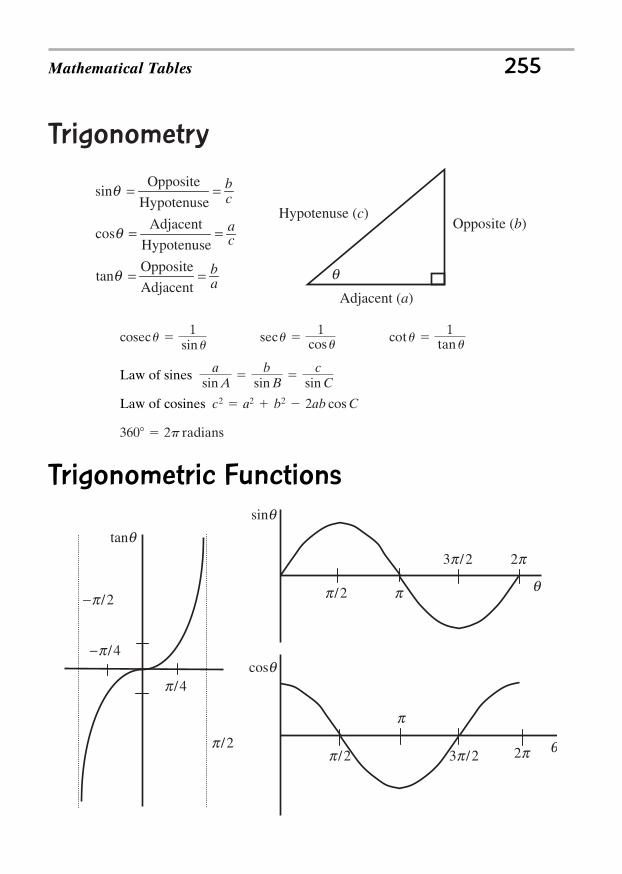
Trigonometry
Mathematical Tables 255
Adjacent (a)
Hypotenuse (c)Opposite (b)
ab
ca
cb
==
==
==
Adjacent
Oppositetanq
Hypotenuse
Adjacentcosq
Hypotenuse
Oppositesinq
q
Law of sines
Law of cosines
Trigonometric Functions
360 2p radians
c2 a2 b2 2ab cos C
asin A
b
sin B
csin C
cosecu 1
sin u secu
1cos u cotu
1tan u
tanq
cosq
sinq
p /2p /2
p /4
- p /4
- p /2 p /2
2p
2p
3p /2
3p /2
p
p
q
q
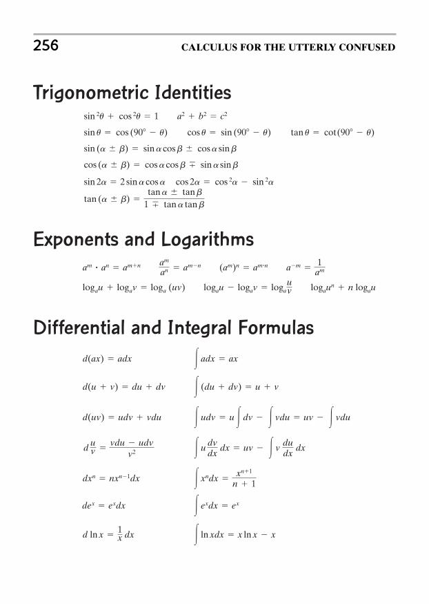
Trigonometric Identities
Exponents and Logarithms
Differential and Integral Formulas
3 ln xdx x ln x xd ln x 1x dx
3 exdx exdex exdx
3 xndx xn1
n 1dxn nxn1dx
3 u dvdx
dx uv 3 v dudx
dxd uv
vdu udvv2
3 udv u 3 dv 3 vdu uv 3 vdud(uv) udv vdu
3 (du dv) u vd(u v) du dv
3 adx axd(ax) adx
logaun n logaulogau logav loga
uvlogau logav loga (uv)
am 1
am(am)n am?nam
an amnam ? an amn
tan (a b) tana tanb
1 7 tana tanb
cos 2a cos 2a sin 2asin 2a 2 sina cosa
cos (a b) cosa cosb 7 sina sinb
sin (a b) sina cosb cosa sinb
tan u cot(90 u)cos u sin (90 u)sin u cos (90 u)
a2 b2 c2sin 2u cos 2u 1
256 CALCULUS FOR THE UTTERLY CONFUSED
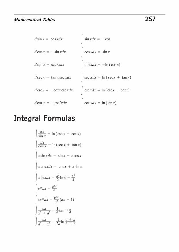
Integral Formulas
3 dxa2 x2
12a
ln a xa x
3 dxx2 a2
1a tan 1 x
a
3 xeaxdx eax
a2 (ax 1)
3 eaxdx eax
a
3 x ln xdx x2
2 ln x x2
4
3 x cos xdx cos x x sin x
3 x sin xdx sin x x cos x
3 dxcos x ln (sec x tan x)
3 dxsin x
ln ( csc x cot x)
3 cot xdx ln ( sin x)d cot x csc2xdx
3 csc xdx ln ( cscx cotx)d cscx cotx csc xdx
3 sec xdx ln ( sec x tan x)d sec x tan x sec xdx
3 tan xdx ln ( cos x)d tan x sec 2xdx
3 cos xdx sin xd cos x sin xdx
3 sin xdx cosd sin x cos xdx
Mathematical Tables 257
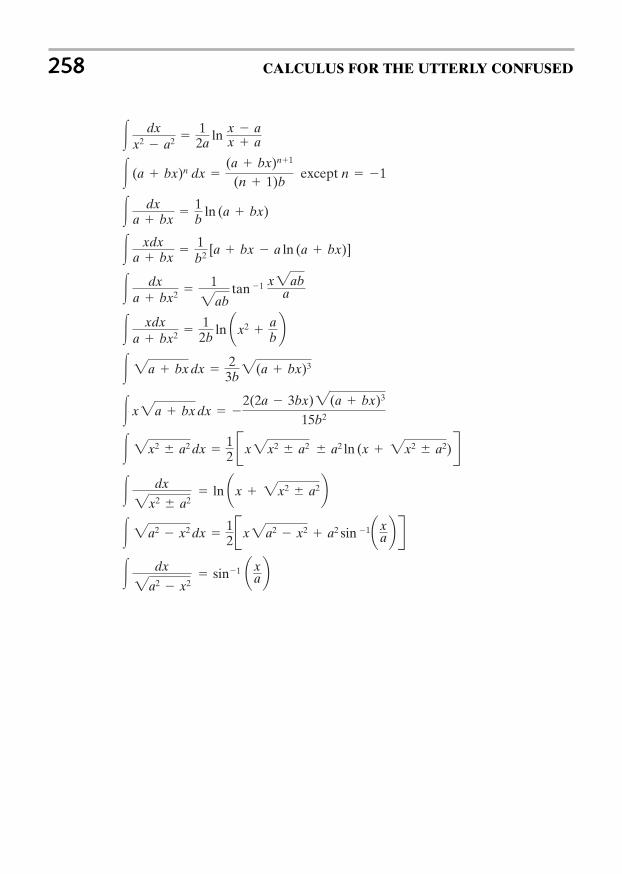
3 dx
2a2 x2 sin1 ¢x
a ≤3 2a2 x2 dx
12Bx2a2 x2 a2 sin 1¢x
a ≤ R3 dx
2x2 a2 ln ¢x 2x2 a2≤
3 2x2 a2 dx 12 Bx2x2 a2 a2 ln (x 2x2 a2)R
3 x2a bx dx 2(2a 3bx)2(a bx)3
15b2
3 2a bx dx 2
3b2(a bx)3
3 xdxa bx2
12b
ln ¢x2 ab≤
3 dxa bx2
1
2abtan 1 x2ab
a
3 xdxa bx
1b2 [a bx a ln (a bx)]
3 dxa bx
1b
ln (a bx)
3 (a bx)n dx (a bx)n1
(n 1)b except n 1
3 dxx2 a2
12a
ln x ax a
258 CALCULUS FOR THE UTTERLY CONFUSED

Index
Copyright © 2007 by The McGraw-Hill Companies, Inc. Click here for terms of use.

This page intentionally left blank
Acceleration, 46, 117Angle:
definition of, 6in degrees, 6, 255in radians, 6
Antiderivative, 114, 116Approximation:
area, 125, 243interest, 190, 246trapezoidal rule, 125, 243
Arc length, 226Area:
under a curve, 123between curves, 130, 139, 173formulas, 254
Asymptotes, 20, 35, 71, 203, 207, 212, 234Average value of a function, 135, 171
Binomial expansion, 4, 254
Chain rule, 53Change of variable, 52Circle, 16Completing the square, 3, 17Compound interest, 190, 246Concavity, 66Congruent triangles, 152Conics:
formulas, 254graphing, 16
Constant of integration, 116
Continuous compounding, 190Coordinate systems, 6Cosine:
definition, 5, 148function, 5, 24, 162law of, 157
Cubic equation, 15Curve sketching, 62
Decay laws, 205Definite integral, 84Derivative:
definition, 42notation, 42power rule, 43of a product, 48of a quotient, 49
Differential:definition, 42formula, 256rules, 43, 48, 49
Discontinuity, 33Disks, method of, 224Doubling time, 207
e, the number, 196Ellipse, 17Equilateral triangles, 153Exponent laws, 9, 181, 256Exponential:
decay, 196
261
Exponential (Cont.):derivative, 187, 189equation, 181function, 181growth, 198
Factorial, 5Factoring, 2First derivative, 63Function:
continuous, 36definition of, 10exponential, 181implicit, 50logarithmic, 193polynomial, 43trigonometric, 5, 23, 255
Geometric formulas, 255Graphing, 61Growth laws, 195, 203, 212
Half-life, 180Horizontal asymptote, 34, 204, 212Hyperbola, 19
Implicit differential, 50Indefinite integral, 114Integral:
definite, 116exponential, 123formulas, 257powers, 115tables of, 242, 256trigonometric, 234
Integration:of exponentials, 188of logarithms, 194numerical, 243by parts, 236by substitution, 229by trapezoidal rule, 243
Interest:compound, 190, 246continuous, 190
Isosceles triangles, 153
Law of cosines, 157Law of exponents, 9, 181, 256
Law of sines, 159Law of supply and demand, 233Learning curve, 204Length of arc, 160Limit, 32Limited growth, 205Limits of integration, 124Line:
equation for, 11intercepts, 11slope, 11
Linear equation, 11Linear function, 11Logarithm:
definitions, 191, 202derivative, 193, 256graph of, 203integral of, 194, 256laws, 9, 191, 256natural, 202
Logistic function, 212
Maximum, 66second derivative, 67
Method:of disks, 224of shells, 223
Minimum, 66second derivative, 67
Motion, 117
Natural logarithm:definition, 202derivative, 193 graph, 150integral, 149
Newton’s law of cooling, 200Numerical integration, 243
Parabola, 12Partial fractions, 171Perimeter formulas, 254Phase, 25Polynomials, 43Power rule:
for differentiation, 43for integration, 115
Product rule, 48Pythagorean theorem, 15, 108
262 INDEX
Quadratic:completing the square, 2equation, 3, 13formula, 2
Quotient rule, 48
Radian, 6 Rational function, 134R-C circuit, 205Related rates, 96R-L circuit, 215
Second derivative, 67Second derivative test, 67Separation of variables, 119Shells, method of, 223Similar triangles, 153Sine:
definition, 5function, 23, 160law of, 159
Slope, 11, 42Spread sheets, 184Substitution method, 229Summation notation, 124
Sums, 243Surface:
area, 228of revolution, 228
Tangent:definition, 5function, 162
Time constant, 207Trapezoidal rule, 123, 243Trigonometric:
definitions, 5, 148, 255differentiation of, 256equations, 168functions, 23, 160identities, 119, 183integration of, 62, 256tables, 170, 257
Variable, change of, 228Velocity, 46, 117Volumes:
by disks, 224formulas, 254by shells, 223
Index 263