what makes expectations great? mdps with bonuses …steele/accesscash/what makes... · what makes...

What Makes Expectations Great?MDPs with Bonuses in the Bargain

J. Michael Steele 1

Wharton SchoolUniversity of Pennsylvania

April 6, 2017

1including joint work with A. Arlotto (Duke) and N. Gans (Wharton)

J.M. Steele (Wharton) MDPs Beyond One’s Means April 6, 2017 1

Some Worrisome Questions with Useful Answers

1 Some Worrisome Questions with Useful Answers

2 Three motivating examples

3 Rich Class of MDPs where Means Bound Variances

4 Beyond Means-Bound-Variances: Sequential Knapsack Problem

5 Markov Additive Functionals of Non-Homogenous MCs — with a Twist

6 Motivating examples: finite-horizon Markov decision problems

7 Dobrushin’s CLT and failure of state-space enlargement

8 MDP Focused Central Limit Theorem

9 Conclusions


Some Worrisome Questions with Useful Answers

What About Expectations and MDPs Were You Afraid to Ask?

Sequential decision problems: The tool of choice is almost always dynamicprogramming and the objective is almost always maximization of an expected reward(or minimization of an expected cost).

In practice, we know dynamic programming often performs admirably. Still, sooneror later, the little voice in our head cannot help but ask, “What about the SaintPetersburg Paradox?”

Nub of the Problem: The realized reward of the decision maker is a random variable,and, for all we know a priori, our myopic focus on means might be disastrous.

Is there an analytical basis for the sensible performance of mean-focused dynamicprogramming?

Our first goal is to isolate a rich class of dynamic programs were the mean-focusedoptimality also guarantees low variability. This is the bonus to our bargain.

Beyond variance bounds, there is the richer goal of limit theorems for the realizedtotal reward. In MDPs there are many sources of dependence and their participationis typically non-linear. This creates a challenging long term agenda. Some concreteprogress has been made.


Three motivating examples









9 Conclusions


Three motivating examples One common question...

Three motivating examples: one common question. . .

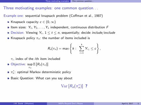
Example one: sequential knapsack problem (Coffman et al., 1987)

Knapsack capacity c ∈ (0,∞)

Item sizes: Y1,Y2, . . . ,Yn independent, continuous distribution F

Decision: Viewing Yt , 1 ≤ t ≤ n, sequentially; decide include/exclude

Knapsack policy πn: the number of items included is

Rn(πn) = max

{k :

k∑i=1

Yτi ≤ c

},

τi , index of the ith item included

Objective: supπn

E [Rn(πn)]

π∗n : optimal Markov deterministic policy

Basic Question: What can you say about

Var [Rn(π∗n)] ?




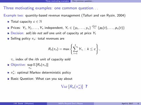
Example two: quantity-based revenue management (Talluri and van Ryzin, 2004)

Total capacity c ∈ N

Prices: Y1,Y2, . . . ,Yn independent, Yt ∈ {y0, . . . , yη}dist∼ {p0(t), . . . , pη(t)}

Decision: sell/do not sell one unit of capacity at price Yt

Selling policy πn: total revenues are

Rn(πn) = max

{k∑

i=1

Yτi : k ≤ c

},

τi , index of the ith unit of capacity sold

Objective: supπn

E [Rn(πn)]



Var [Rn(π∗n)] ?




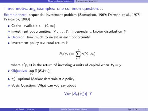
Example three: sequential investment problem (Samuelson, 1969; Derman et al., 1975;Prastacos, 1983)

Capital available c ∈ (0,∞)

Investment opportunities: Y1, . . . ,Yn, independent, known distribution F

Decision: how much to invest in each opportunity

Investment policy πn: total return is

Rn(πn) =n∑

t=1

r(Yt ,At),

where r(y , a) is the return of investing a units of capital when Yt = y

Objective: supπn

E [Rn(πn)]



Var [Rn(π∗n)] ?


Three motivating examples What Do We Gain?

What Do We Gain From Understanding Var [Rn(π∗n)] ?

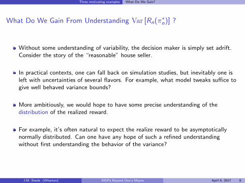
Without some understanding of variability, the decision maker is simply set adrift.Consider the story of the “reasonable” house seller.

In practical contexts, one can fall back on simulation studies, but inevitably one isleft with uncertainties of several flavors. For example, what model tweaks suffice togive well behaved variance bounds?

More ambitiously, we would hope to have some precise understanding of thedistribution of the realized reward.

For example, it’s often natural to expect the realize reward to be asymptoticallynormally distributed. Can one have any hope of such a refined understandingwithout first understanding the behavior of the variance?


Three motivating examples Good Behavior of the Example MDPs

Good Behavior of the Example MDPs

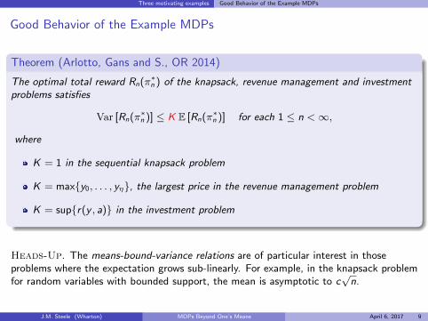
Theorem (Arlotto, Gans and S., OR 2014)

The optimal total reward Rn(π∗n ) of the knapsack, revenue management and investmentproblems satisfies

Var [Rn(π∗n )] ≤ K E [Rn(π∗n )] for each 1 ≤ n <∞,

where

K = 1 in the sequential knapsack problem

K = max{y0, . . . , yη}, the largest price in the revenue management problem

K = sup{r(y , a)} in the investment problem

Heads-Up. The means-bound-variance relations are of particular interest in thoseproblems where the expectation grows sub-linearly. For example, in the knapsack problemfor random variables with bounded support, the mean is asymptotic to c

√n.


Three motivating examples Good Behavior of the Example MDPs

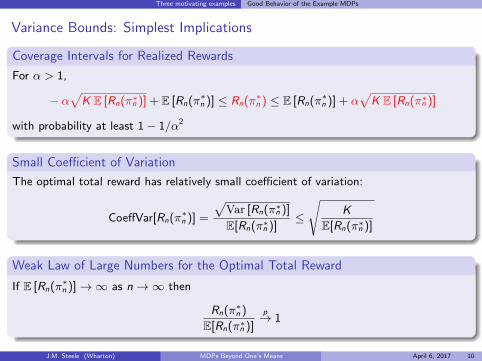
Variance Bounds: Simplest Implications

Coverage Intervals for Realized Rewards

For α > 1,

− α√

K E [Rn(π∗n )] + E [Rn(π∗n )] ≤ Rn(π∗n ) ≤ E [Rn(π∗n )] + α√

K E [Rn(π∗n )]

with probability at least 1− 1/α2

Small Coefficient of Variation

The optimal total reward has relatively small coefficient of variation:

CoeffVar[Rn(π∗n )] =

√Var [Rn(π∗n )]

E[Rn(π∗n )]≤

√K

E[Rn(π∗n )]

Weak Law of Large Numbers for the Optimal Total Reward

If E [Rn(π∗n )]→∞ as n→∞ then

Rn(π∗n )

E[Rn(π∗n )]

p→ 1


Rich Class of MDPs where Means Bound Variances









9 Conclusions


Rich Class of MDPs where Means Bound Variances General MDP Framework

General MDP Framework

(X , Y , A , f , r , n

)X is the state space; at each t the DM knows the state of the system x ∈ X

I Knapsack example: x is the remaining capacity

The independent sequence Y1,Y2, . . .Yn takes value in YI Knapsack example: y ∈ Y is the size of the item that is presented

Action space: A(t, x , y) ⊆ A is the set of admissible actions for (x , y) at tI Knapsack example: “select”; “do not select”

State transition function: f (t, x , y , a) state that one reaches for a ∈ A(t, x , y)I Knapsack example: f (t, x , y , select) = x− y; f (t, x , y ,do not select) = x

Reward function: r(t, x , y , a) reward for taking action a at time t when at (x , y)I Knapsack example: r(t, x , y , select) = 1; r(t, x , y , do not select) = 0

Time horizon: n <∞


Rich Class of MDPs where Means Bound Variances General MDP Framework

MDPs where Means Bound Variances

Π(n) set of all feasible Markov deterministic policies for the n-period problem

Reward of policy π up to time k

Rk(π) =k∑

t=1

r(t,Xt ,Yt ,At), X1 = x̄ , 1 ≤ k ≤ n

Expected total reward criterion, i.e. we are looking for π∗n ∈ Π(n) such that

E[Rn(π∗n )] = supπ∈Π(n)

E[Rn(π)].

Bellman equation: for each 1 ≤ t ≤ n and for x ∈ X ,

vt(x) = E

[sup

a∈A(t,x,Yt )

{r(t, x ,Yt , a) + vt+1 (f (t, x ,Yt , a))}

],

I vn+1(x) = 0 for all x ∈ X , andI v1(x̄) = E[Rn(π∗n )]


Rich Class of MDPs where Means Bound Variances Three Basic Properties

Three Basic Properties

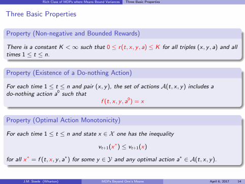
Property (Non-negative and Bounded Rewards)

There is a constant K <∞ such that 0 ≤ r(t, x , y , a) ≤ K for all triples (x , y , a) and alltimes 1 ≤ t ≤ n.

Property (Existence of a Do-nothing Action)

For each time 1 ≤ t ≤ n and pair (x , y), the set of actions A(t, x , y) includes ado-nothing action a0 such that

f (t, x , y , a0) = x

Property (Optimal Action Monotonicity)

For each time 1 ≤ t ≤ n and state x ∈ X one has the inequality

vt+1(x∗) ≤ vt+1(x)

for all x∗ = f (t, x , y , a∗) for some y ∈ Y and any optimal action a∗ ∈ A(t, x , y).


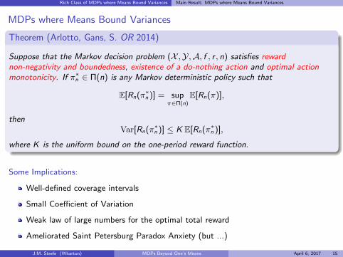
Rich Class of MDPs where Means Bound Variances Main Result: MDPs where Means Bound Variances

MDPs where Means Bound Variances

Theorem (Arlotto, Gans, S. OR 2014)

Suppose that the Markov decision problem (X ,Y,A, f , r , n) satisfies rewardnon-negativity and boundedness, existence of a do-nothing action and optimal actionmonotonicity. If π∗n ∈ Π(n) is any Markov deterministic policy such that

E[Rn(π∗n )] = supπ∈Π(n)

E[Rn(π)],

thenVar[Rn(π∗n )] ≤ K E[Rn(π∗n )],

where K is the uniform bound on the one-period reward function.

Some Implications:

Well-defined coverage intervals

Small Coefficient of Variation

Weak law of large numbers for the optimal total reward

Ameliorated Saint Petersburg Paradox Anxiety (but ...)


Rich Class of MDPs where Means Bound Variances Understanding the Three Crucial Properties

Understanding the Three Crucial Properties

In summary, the variance of the optimal total reward is “small” provided that we havethe three conditions: . . .

Property 1: Non-negative and bounded rewards

Property 2: Existence of a do-nothing action

Property 3: Optimal action monotonicity, vt+1(x∗) ≤ vt+1(x)

Are these easy to check? Fortunately, the answer is “Yes.”


Rich Class of MDPs where Means Bound Variances Optimal action monotonicity: sufficient conditions

Optimal action monotonicity: sufficient conditions

Sufficient Conditions

A Markov decision problem (X ,Y,A, f , r , n) satisfies optimal action monotonicity if:

(i) the state space X is a subset of a finite-dimensional Euclidean space equipped witha partial order �;

(ii) for each y ∈ Y, 1 ≤ t ≤ n and each optimal action a∗ ∈ A(t, x , y) one hasf (t, x , y , a∗) ≡ x∗ � x

(iii) for each 1 ≤ t ≤ n, the map x 7→ vt(x) is non-decreasing: i.e. x � x ′ impliesvt(x) ≤ vt(x

′);

Remark

Analogously, one can require that

(ii) x � x∗ ≡ f (t, x , y , a∗);

(iii) the map x 7→ vt(x) is non-increasing: i.e. x � x ′ implies vt(x′) ≤ vt(x).


Rich Class of MDPs where Means Bound Variances Optimal action monotonicity: sufficient conditions

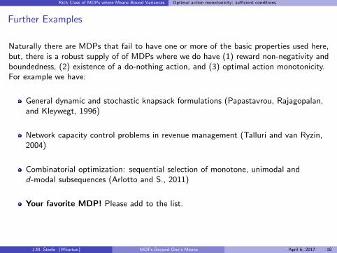
Further Examples

Naturally there are MDPs that fail to have one or more of the basic properties used here,but, there is a robust supply of of MDPs where we do have (1) reward non-negativity andboundedness, (2) existence of a do-nothing action, and (3) optimal action monotonicity.For example we have:

General dynamic and stochastic knapsack formulations (Papastavrou, Rajagopalan,and Kleywegt, 1996)

Network capacity control problems in revenue management (Talluri and van Ryzin,2004)

Combinatorial optimization: sequential selection of monotone, unimodal andd-modal subsequences (Arlotto and S., 2011)

Your favorite MDP! Please add to the list.


Rich Class of MDPs where Means Bound Variances Two Variations on the MDP Framework

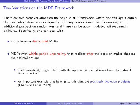
Two Variations on the MDP Framework

There are two basic variations on the basic MDP Framework, where one can again obtainthe means-bound-variances inequality. In many contexts one has discounting oradditional post-action randomness, and these can be accommodated without muchdifficulty. Specifically, one can deal with

Finite horizon discounted MDPs

MDPs with within-period uncertainty that realizes after the decision maker choosesthe optimal action:

I Such uncertainty might affect both the optimal one-period reward and the optimalstate-transition

I An important example that belongs to this class are stochastic depletion problems(Chan and Farias, 2009)


Beyond Means-Bound-Variances: Sequential Knapsack Problem









9 Conclusions


Beyond Means-Bound-Variances: Sequential Knapsack Problem Sharper Focus

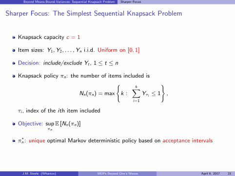
Sharper Focus: The Simplest Sequential Knapsack Problem

Knapsack capacity c = 1

Item sizes: Y1,Y2, . . . ,Yn i.i.d. Uniform on [0, 1]

Decision: include/exclude Yt , 1 ≤ t ≤ n

Knapsack policy πn: the number of items included is

Nn(πn) = max

{k :

k∑i=1

Yτi ≤ 1

},

τi , index of the ith item included

Objective: supπn

E [Nn(πn)]

π∗n : unique optimal Markov deterministic policy based on acceptance intervals


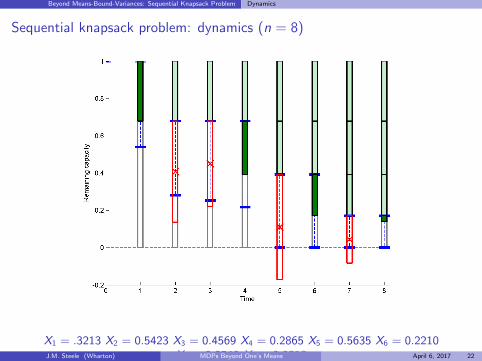
Beyond Means-Bound-Variances: Sequential Knapsack Problem Dynamics

Sequential knapsack problem: dynamics (n = 8)

X1 = .3213 X2 = 0.5423 X3 = 0.4569 X4 = 0.2865 X5 = 0.5635 X6 = 0.2210X7 = 0.2540 X8 = 0.0318J.M. Steele (Wharton) MDPs Beyond One’s Means April 6, 2017 22

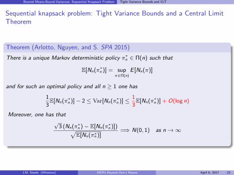
Beyond Means-Bound-Variances: Sequential Knapsack Problem Tight Variance Bounds and CLT

Sequential knapsack problem: Tight Variance Bounds and a Central LimitTheorem

Theorem (Arlotto, Nguyen, and S. SPA 2015)

There is a unique Markov deterministic policy π∗n ∈ Π(n) such that

E[Nn(π∗n )] = supπ∈Π(n)

E [Nn(π)]

and for such an optimal policy and all n ≥ 1 one has

1

3E[Nn(π∗n )]− 2 ≤ Var[Nn(π∗n )] ≤ 1

3E[Nn(π∗n )] + O(log n)

Moreover, one has that√

3 (Nn(π∗n )− E[Nn(π∗n )])√E[Nn(π∗n )]

=⇒ N(0, 1) as n→∞


Beyond Means-Bound-Variances: Sequential Knapsack Problem Tight Variance Bounds and CLT

Observations on the Knapsack CLT

The central limit theorem holds despite strong dependence on the level of remainingcapacity and on the time period

Asymptotic normality tells us almost everything we would like to know!

Intriguing Open Issue: How is does the central limit theorem for the knapsackdepend on the distribution F . This appears to be quite delicate.

Major Issue:

In what contexts can we get a CLT for the realized reward of an MDP? Is thisalways an issue of specific problems, or is there some kind of CLT that is relevant toa large class of MDPs. The essence of the matter seems to pivot on the possibilityof useful CLTs for non-homogenous Markov additive functionals.


Markov Additive Functionals of Non-Homogenous MCs — with a Twist









9 Conclusions


Markov Additive Functionals of Non-Homogenous MCs — with a Twist

Markov Additive Functionals — Plus m

Here we are concerned with the possibility of an Asymptotic Gaussian law for partialsums of the form:

Sn =n∑

i=1

fn,i (Xn,i , . . . ,Xn,i+m), for n ≥ 1

Framework:

{Xn,i : 1 ≤ i ≤ n + m} are n + m observations from a time non-homogeneousMarkov chain with general state space X

{fn,i : 1 ≤ i ≤ n} are real-valued functions on X 1+m

m ≥ 0: novel twist

Why m?


Motivating examples









9 Conclusions


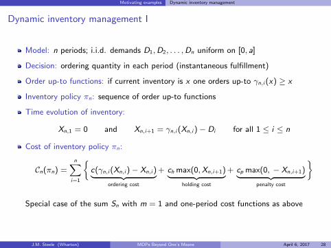
Motivating examples Dynamic inventory management

Dynamic inventory management I

Model: n periods; i.i.d. demands D1,D2, . . . ,Dn uniform on [0, a]

Decision: ordering quantity in each period (instantaneous fulfillment)

Order up-to functions: if current inventory is x one orders up-to γn,i (x) ≥ x

Inventory policy πn: sequence of order up-to functions

Time evolution of inventory:

Xn,1 = 0 and Xn,i+1 = γn,i (Xn,i )− Di for all 1 ≤ i ≤ n

Cost of inventory policy πn:

Cn(πn) =n∑

i=1

{c(γn,i (Xn,i )− Xn,i )︸︷︷︸

ordering cost

+ ch max(0,Xn,i+1)︸︷︷︸holding cost

+ cp max(0, − Xn,i+1)︸︷︷︸penalty cost

}

Special case of the sum Sn with m = 1 and one-period cost functions as above


Motivating examples Dynamic inventory management

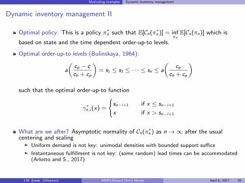
Dynamic inventory management II

Optimal policy: This is a policy π∗n such that E[Cn(π∗n )] = infπn

E[Cn(πn)] which is

based on state and the time dependent order-up-to levels.

Optimal order-up-to levels (Bulinskaya, 1964):

a

(cp − c

ch + cp

)= s1 ≤ s2 ≤ · · · ≤ sn ≤ a

(cp

ch + cp

)

such that the optimal order-up-to function

γ∗n,i (x) =

{sn−i+1 if x ≤ sn−i+1

x if x > sn−i+1

What are we after? Asymptotic normality of Cn(π∗n ) as n→∞ after the usualcentering and scaling

I Uniform demand is not key: unimodal densities with bounded support suffice

I Instantaneous fulfillment is not key: (some random) lead times can be accommodated(Arlotto and S., 2017)


Dobrushin’s CLT and failure of state-space enlargement









9 Conclusions


Dobrushin’s CLT and failure of state-space enlargement The minimal ergodic coefficient

The minimal ergodic coefficient

Dobrushin contraction coefficient: Given a Markov transition kernel K ≡ K(x , dy)on X , the Dobrushin contraction coefficient of K is given by

δ(K) = supx1,x2∈X

||K(x1, ·)− K(x2, ·)||TV = supx1,x2∈XB∈B(X )

|K(x1,B)− K(x2,B)|

Ergodic coefficient:α(K) = 1− δ(K)

Minimal ergodic coefficient: Given a time non-homogeneous Markov chain{X̂n,i : 1 ≤ i ≤ n} one has the Markov transition kernels

K(n)i,i+1(x ,B) = P(X̂n,i+1 ∈ B | X̂n,i = x), 1 ≤ i < n,

and the minimal ergodic coefficient is given by

αn = min1≤i<n

α(K(n)i,i+1)


Dobrushin’s CLT and failure of state-space enlargement Dobrushin’s CLT

A building block: Dobrushin’s central limit theorem

Theorem (Dobrushin, 1956; see also Sethuraman and Varadhan, 2005)

For each n ≥ 1, let {X̂n,i : 1 ≤ i ≤ n} be n observations of a non-homogeneous Markovchain. If

Sn =n∑

i=1

fn,i (X̂n,i )

and if there are constants C1,C2, . . . such that

max1≤i≤n

||fn,i ||∞ ≤ Cn and limn→∞

C 2n

α3n

(∑ni=1 Var[fn,i (X̂n,i )]

) = 0,

then one has the convergence in distribution

Sn − E[Sn]√Var[Sn]

=⇒ N(0, 1), as n→∞

Role of the minimal ergodic coefficient αn


Dobrushin’s CLT and failure of state-space enlargement Dobrushin’s CLT

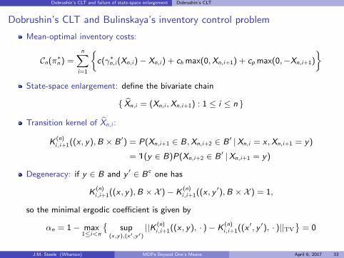
Dobrushin’s CLT and Bulinskaya’s inventory control problem

Mean-optimal inventory costs:

Cn(π∗n ) =n∑

i=1

{c(γ∗n,i (Xn,i )− Xn,i ) + ch max(0,Xn,i+1) + cp max(0,−Xn,i+1)

}State-space enlargement: define the bivariate chain

{ X̂n,i = (Xn,i ,Xn,i+1) : 1 ≤ i ≤ n }

Transition kernel of X̂n,i :

K(n)i,i+1((x , y),B × B ′) = P(Xn,i+1 ∈ B,Xn,i+2 ∈ B ′ |Xn,i = x ,Xn,i+1 = y)

= 1(y ∈ B)P(Xn,i+2 ∈ B ′ |Xn,i+1 = y)

Degeneracy: if y ∈ B and y ′ ∈ Bc one has

K(n)i,i+1((x , y),B ×X )− K

(n)i,i+1((x , y ′),B ×X ) = 1,

so the minimal ergodic coefficient is given by

αn = 1− max1≤i<n

{sup

(x,y),(x′,y′)

||K (n)i,i+1((x , y), · )− K

(n)i,i+1((x ′, y ′), · )||TV

}= 0


MDP Focused Central Limit Theorem









9 Conclusions


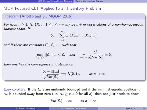
MDP Focused Central Limit Theorem MDP Focused Markov Additive CLT

MDP Focused Markov Additive CLT

Theorem (Arlotto and S., MOOR, 2016)

For each n ≥ 1, let {Xn,i : 1 ≤ i ≤ n + m} be n + m observations of a non-homogeneousMarkov chain. If

Sn =n∑

i=1

fn,i (Xn,i , . . . ,Xn,i+m)


max1≤i≤n


C 2n

α2nVar[Sn]

= 0,



=⇒ N(0, 1), as n→∞

Easy corollary: If the Cn’s are uniformly bounded and if the minimal ergodic coefficientαn is bounded away from zero (i.e. αn ≥ c > 0 for all n), then one just needs to show

Var[Sn]→∞ as n→∞


MDP Focused Central Limit Theorem Comparison of conditions

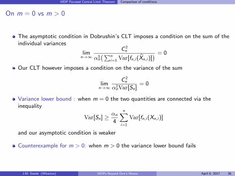
On m = 0 vs m > 0

The asymptotic condition in Dobrushin’s CLT imposes a condition on the sum of theindividual variances

limn→∞

C 2n

α3n

(∑ni=1 Var[fn,i (X̂n,i )]

) = 0

Our CLT however imposes a condition on the variance of the sum

limn→∞

C 2n

α2nVar[Sn]

= 0

Variance lower bound : when m = 0 the two quantities are connected via theinequality

Var[Sn] ≥ αn

4

n∑i=1

Var[fn,i (Xn,i )]

and our asymptotic condition is weaker

Counterexample for m > 0: when m > 0 the variance lower bound fails


MDP Focused Central Limit Theorem Counterexample to variance lower bound

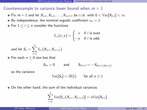
Counterexample to variance lower bound when m = 1

Fix m = 1 and let Xn,1,Xn,2, . . . ,Xn,n+1 be i.i.d. with 0 < Var[Xn,1] <∞By independence, the minimal ergodic coefficient αn = 1

For 1 ≤ i ≤ n consider the functions

fn,i (x , y) =

{x if i is even

−y if i is odd;

and let Sn =n∑

i=1

fn,i (Xn,i ,Xn,i+1)

For each n ≥ 0 one has that

S2n = 0 and S2n+1 = −X2n+1,2(n+1)

so the varianceVar[Sn] = O(1) for all n ≥ 1

On the other hand, the sum of the individual variances

n∑i=1

Var[fn,i (Xn,i ,Xn,i+1)] = nVar[Xn,1]


MDP Focused Central Limit Theorem Back to the Inventory Example

MDP Focused CLT Applied to an Inventory Problem

Theorem (Arlotto and S., MOOR, 2016)

For each n ≥ 1, let {Xn,i : 1 ≤ i ≤ n + m} be n + m observations of a non-homogeneousMarkov chain. If

Sn =n∑

i=1

fn,i (Xn,i , . . . ,Xn,i+m)


max1≤i≤n


C 2n

α2nVar[Sn]

= 0,



=⇒ N(0, 1), as n→∞

Easy corollary: If the Cn’s are uniformly bounded and if the minimal ergodic coefficientαn is bounded away from zero (i.e. αn ≥ c > 0 for all n), then one just needs to show

Var[Sn]→∞ as n→∞


MDP Focused Central Limit Theorem Back to the Inventory Example

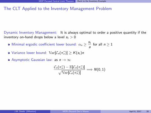
The CLT Applied to the Inventory Management Problem

Dynamic Inventory Management: It is always optimal to order a positive quantity if theinventory on-hand drops below a level s1 > 0

Minimal ergodic coefficient lower bound: αn ≥s1

afor all n ≥ 1

Variance lower bound: Var[Cn(π∗n )] ≥ K(s1)n

Asymptotic Gaussian law: as n→∞

Cn(π∗n )− E[Cn(π∗n )]√Var[Cn(π∗n )]

=⇒ N(0, 1)


Conclusions









9 Conclusions


Conclusions

Summary

Main Message: One need not feel too guilty applying mean-focused MDP tools.We know they seem to work in practice, and there is a growing body of knowledgethat helps to explain why they work.

First: In a rich class of problems, there are a priori bounds on the variance that aregiven in terms of the mean reward and the bound on the individual rewards.

Three simple properties characterize this class.

Second: When more information is available on the Markov chain of decision statesand post-decision reward functions, one has good prospects for a Central LimitTheorem.

Application of the MDP focused CLT is not work-free. Nevertheless, because of theMDP focus, one has a much shorter path to a CLT than one could realisticallyexpect otherwise. At a minimum, we know reasonably succinct sufficient conditionsfor a CLT.


Thank you!


Proof Detail: MDPs where Means Bound Variances Proof Details

Bounding the variance by the mean: proof details

The martingale difference

dt = Mt −Mt−1 = r(t,Xt ,Yt ,A∗t ) + vt+1(Xt+1)− vt(Xt)

Add and subtract vt+1(Xt) to obtain

dt = vt+1(Xt)− vt(Xt)

+ r(t,Xt ,Yt ,A∗t ) + vt+1(X ∗t+1)− vt+1(Xt)

Recall: Xt is Ft−1-measurable

Hence, αt is Ft−1-measurable and αt = −E[βt | Ft−1], so

E[d2t | Ft−1] = E[β2

t | Ft−1] + 2αtE[βt | Ft−1] + α2t = E[β2

t | Ft−1]− α2t

Since α2t ≥ 0 and βt ≤ r(t,Xt ,Yt ,A

∗t )

E[d2t | Ft−1] ≤ E[β2

t | Ft−1] ≤ K E[r(t,Xt ,Yt ,A∗t ) | Ft−1]

Back to Proof Sketch


Proof Detail: MDPs where Means Bound Variances Proof

Bounding the variance by the mean: proof sketch

For 0 ≤ t ≤ n, the process

Mt = Rt(π∗n ) + vt+1(Xt+1)

is a martingale with respect to the natural filtration Ft = σ{Y1, . . . ,Yt}

M0 = E[Rn(π∗n )] and Mn = Rn(π∗n )

For dt = Mt −Mt−1,

Var[Mn] = Var [Rn(π∗n )] = E

[n∑

t=1

d2t

]

“Some rearranging” and an application of reward non-negativity and boundedness,existence of a do-nothing action, and optimal action monotonicity gives

E[d2t | Ft−1] ≤ K E[r(t,Xt ,Yt ,A

∗t ) | Ft−1]

Taking total expectations and summing gives

Var [Rn(π∗n )] ≤ K E [Rn(π∗n )]

Crucial here: Xt+1 = f (t,Xt ,Yt ,At) is Ft-measurable!


Proof Detail: MDPs where Means Bound Variances Proof

Bounding the variance by the mean: proof details

The martingale difference

dt = Mt −Mt−1 = r(t,Xt ,Yt ,A∗t ) + vt+1(Xt+1)− vt(Xt)

Add and subtract vt+1(Xt) to obtain

dt =

αt︷︸︸︷vt+1(Xt)− vt(Xt)

+ r(t,Xt ,Yt ,A∗t ) + vt+1(Xt+1)− vt+1(Xt)︸︷︷︸

βt

Recall: Xt is Ft−1-measurable

Hence, αt is Ft−1-measurable and αt = −E[βt | Ft−1], so

E[d2t | Ft−1] = E[β2

t | Ft−1] + 2αtE[βt | Ft−1] + α2t = E[β2

t | Ft−1]− α2t

Since α2t ≥ 0 and βt ≤ r(t,Xt ,Yt ,A

∗t )

E[d2t | Ft−1] ≤ E[β2

t | Ft−1] ≤ K E[r(t,Xt ,Yt ,A∗t ) | Ft−1]


Proof Detail: MDPs where Means Bound Variances Uniform boundedness

Remark (Uniform Boundedness)

The Variance Bound still holds if there is a constant K <∞ such that

E[r 2(t,Xt ,Yt ,A∗t )] ≤ KE[r(t,Xt ,Yt ,A

∗t )]

uniformly in t.


Proof Detail: MDPs where Means Bound Variances Bounded martingale differences

Remark (Bounded Differences Martingale)

The Bellman martingale has bounded differences. In fact we also have that

|dt | = |Mt −Mt−1| = |αt + βt | ≤ K

for all 1 ≤ t ≤ n.


References

References I

Alessandro Arlotto and J. Michael Steele. Optimal sequential selection of a unimodalsubsequence of a random sequence. Combinatorics, Probability and Computing, 20(06):799–814, 2011. doi: 10.1017/S0963548311000411.

Carri W. Chan and Vivek F. Farias. Stochastic depletion problems: effective myopicpolicies for a class of dynamic optimization problems. Math. Oper. Res., 34(2):333–350, 2009. ISSN 0364-765X. doi: 10.1287/moor.1080.0364. URLhttp://dx.doi.org/10.1287/moor.1080.0364.

E. G. Coffman, Jr., L. Flatto, and R. R. Weber. Optimal selection of stochastic intervalsunder a sum constraint. Adv. in Appl. Probab., 19(2):454–473, 1987. ISSN 0001-8678.doi: 10.2307/1427427.

C. Derman, G. J. Lieberman, and S. M. Ross. A stochastic sequential allocation model.Operations Res., 23(6):1120–1130, 1975. ISSN 0030-364X.

Jason D. Papastavrou, Srikanth Rajagopalan, and Anton J. Kleywegt. The dynamic andstochastic knapsack problem with deadlines. Management Science, 42(12):1706–1718,1996. ISSN 00251909.

Gregory P. Prastacos. Optimal sequential investment decisions under conditions ofuncertainty. Management Science, 29(1):118–134, 1983. ISSN 00251909.


http://dx.doi.org/10.1287/moor.1080.0364

References

References II

Paul A. Samuelson. Lifetime portfolio selection by dynamic stochastic programming. TheReview of Economics and Statistics, 51(3):239–246, 1969. ISSN 00346535.

Kalyan T. Talluri and Garrett J. van Ryzin. The theory and practice of revenuemanagement. International Series in Operations Research & Management Science, 68.Kluwer Academic Publishers, Boston, MA, 2004. ISBN 1-4020-7701-7.


what makes expectations great? mdps with bonuses …steele/accesscash/what makes... · what makes...

Documents