what is digital signal processing? · 2008-08-28 · digital signal processing is aﬂavor of...

Chapter 1

What Is Digital Signal Processing?

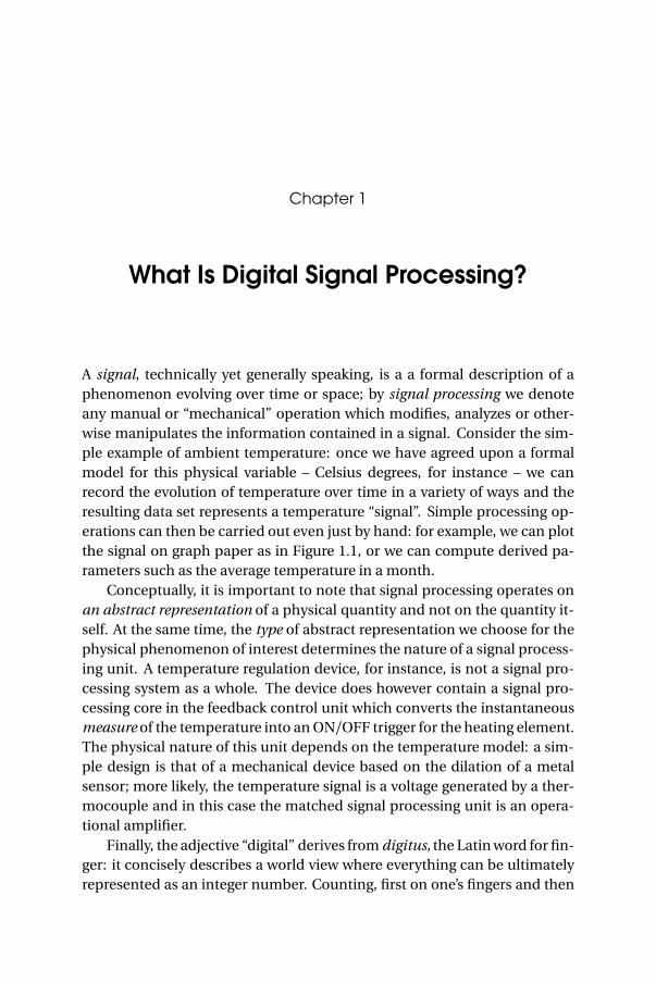
A signal, technically yet generally speaking, is a a formal description of aphenomenon evolving over time or space; by signal processing we denoteany manual or “mechanical” operation which modifies, analyzes or other-wise manipulates the information contained in a signal. Consider the sim-ple example of ambient temperature: once we have agreed upon a formalmodel for this physical variable – Celsius degrees, for instance – we canrecord the evolution of temperature over time in a variety of ways and theresulting data set represents a temperature “signal”. Simple processing op-erations can then be carried out even just by hand: for example, we can plotthe signal on graph paper as in Figure 1.1, or we can compute derived pa-rameters such as the average temperature in a month.

Conceptually, it is important to note that signal processing operates onan abstract representation of a physical quantity and not on the quantity it-self. At the same time, the type of abstract representation we choose for thephysical phenomenon of interest determines the nature of a signal process-ing unit. A temperature regulation device, for instance, is not a signal pro-cessing system as a whole. The device does however contain a signal pro-cessing core in the feedback control unit which converts the instantaneousmeasure of the temperature into an ON/OFF trigger for the heating element.The physical nature of this unit depends on the temperature model: a sim-ple design is that of a mechanical device based on the dilation of a metalsensor; more likely, the temperature signal is a voltage generated by a ther-mocouple and in this case the matched signal processing unit is an opera-tional amplifier.

Finally, the adjective “digital” derives from digitus, the Latin word for fin-ger: it concisely describes a world view where everything can be ultimatelyrepresented as an integer number. Counting, first on one’s fingers and then

2 Some History and Philosophy

5

10

15

0 10 20 30

��

� � ��

��

��

��

��

��

� � ��

�

�

�

[◦C]

Figure 1.1 Temperature measurements over a month.

in one’s head, is the earliest and most fundamental form of abstraction; aschildren we quickly learn that counting does indeed bring disparate objects(the proverbial “apples and oranges”) into a common modeling paradigm,i.e. their cardinality. Digital signal processing is a flavor of signal processingin which everything including time is described in terms of integer num-bers; in other words, the abstract representation of choice is a one-size-fit-all countability. Note that our earlier “thought experiment” about ambienttemperature fits this paradigm very naturally: the measuring instants forma countable set (the days in a month) and so do the measures themselves(imagine a finite number of ticks on the thermometer’s scale). In digitalsignal processing the underlying abstract representation is always the setof natural numbers regardless of the signal’s origins; as a consequence, thephysical nature of the processing device will also always remain the same,that is, a general digital (micro)processor. The extraordinary power and suc-cess of digital signal processing derives from the inherent universality of itsassociated “world view”.

1.1 Some History and Philosophy

1.1.1 Digital Signal Processing under the Pyramids

Probably the earliest recorded example of digital signal processing datesback to the 25th century BC. At the time, Egypt was a powerful kingdomreaching over a thousand kilometers south of the Nile’s delta. For all itslatitude, the kingdom’s populated area did not extend for more than a fewkilometers on either side of the Nile; indeed, the only inhabitable areas inan otherwise desert expanse were the river banks, which were made fertile

What Is Digital Signal Processing? 3

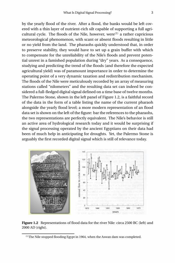
by the yearly flood of the river. After a flood, the banks would be left cov-ered with a thin layer of nutrient-rich silt capable of supporting a full agri-cultural cycle. The floods of the Nile, however, were(1) a rather capriciousmeteorological phenomenon, with scant or absent floods resulting in littleor no yield from the land. The pharaohs quickly understood that, in orderto preserve stability, they would have to set up a grain buffer with whichto compensate for the unreliability of the Nile’s floods and prevent poten-tial unrest in a famished population during “dry” years. As a consequence,studying and predicting the trend of the floods (and therefore the expectedagricultural yield) was of paramount importance in order to determine theoperating point of a very dynamic taxation and redistribution mechanism.The floods of the Nile were meticulously recorded by an array of measuringstations called “nilometers” and the resulting data set can indeed be con-sidered a full-fledged digital signal defined on a time base of twelve months.The Palermo Stone, shown in the left panel of Figure 1.2, is a faithful recordof the data in the form of a table listing the name of the current pharaohalongside the yearly flood level; a more modern representation of an flooddata set is shown on the left of the figure: bar the references to the pharaohs,the two representations are perfectly equivalent. The Nile’s behavior is stillan active area of hydrological research today and it would be surprising ifthe signal processing operated by the ancient Egyptians on their data hadbeen of much help in anticipating for droughts. Yet, the Palermo Stone isarguably the first recorded digital signal which is still of relevance today.

Figure 1.2 Representations of flood data for the river Nile: circa 2500 BC (left) and2000 AD (right).

(1)The Nile stopped flooding Egypt in 1964, when the Aswan dam was completed.


1.1.2 The Hellenic Shift to Analog Processing

“Digital” representations of the world such as those depicted by the PalermoStone are adequate for an environment in which quantitative problems aresimple: counting cattle, counting bushels of wheat, counting days and soon. As soon as the interaction with the world becomes more complex, sonecessarily do the models used to interpret the world itself. Geometry, forinstance, is born of the necessity of measuring and subdividing land prop-erty. In the act of splitting a certain quantity into parts we can already seethe initial difficulties with an integer-based world view ;(2) yet, until the Hel-lenic period, western civilization considered natural numbers and their ra-tios all that was needed to describe nature in an operational fashion. In the6th century BC, however, a devastated Pythagoras realized that the the sideand the diagonal of a square are incommensurable, i.e. that

�2 is not a sim-

ple fraction. The discovery of what we now call irrational numbers “sealedthe deal” on an abstract model of the world that had already appeared inearly geometric treatises and which today is called the continuum. Heavilysteeped in its geometric roots (i.e. in the infinity of points in a segment), thecontinuum model postulates that time and space are an uninterrupted flowwhich can be divided arbitrarily many times into arbitrarily (and infinitely)small pieces. In signal processing parlance, this is known as the “analog”world model and, in this model, integer numbers are considered primitiveentities, as rough and awkward as a set of sledgehammers in a watchmaker’sshop.

In the continuum, the infinitely big and the infinitely small dance to-gether in complex patterns which often defy our intuition and which re-quired almost two thousand years to be properly mastered. This is of coursenot the place to delve deeper into this extremely fascinating epistemologi-cal domain; suffice it to say that the apparent incompatibility between thedigital and the analog world views appeared right from the start (i.e. fromthe 5th century BC) in Zeno’s works; we will appreciate later the immenseimport that this has on signal processing in the context of the sampling the-orem.

Zeno’s paradoxes are well known and they underscore this unbridgeablegap between our intuitive, integer-based grasp of the world and a model of

(2)The layman’s aversion to “complicated” fractions is at the basis of many counting sys-tems other than the decimal (which is just an accident tied to the number of human fin-gers). Base-12 for instance, which is still so persistent both in measuring units (hours ina day, inches in a foot) and in common language (“a dozen”) originates from the simplefact that 12 happens to be divisible by 2, 3 and 4, which are the most common numberof parts an item is usually split into. Other bases, such as base-60 and base-360, haveemerged from a similar abundance of simple factors.


the world based on the continuum. Consider for instance the dichotomyparadox; Zeno states that if you try to move along a line from point A topoint B you will never in fact be able to reach your destination. The rea-soning goes as follows: in order to reach B, you will have to first go throughpoint C, which is located mid-way between A and B; but, even before youreach C, you will have to reach D, which is the midpoint between A and C;and so on ad infinitum. Since there is an infinity of such intermediate points,Zeno argues, moving from A to B requires you to complete an infinite num-ber of tasks, which is humanly impossible. Zeno of course was well awareof the empirical evidence to the contrary but he was brilliantly pointing outthe extreme trickery of a model of the world which had not yet formally de-fined the concept of infinity. The complexity of the intellectual machineryneeded to solidly counter Zeno’s argument is such that even today the para-dox is food for thought. A first-year calculus student may be tempted tooffhandedly dismiss the problem by stating

∞∑n=1

1

2n = 1 (1.1)

but this is just a void formalism begging the initial question if the underlyingnotion of the continuum is not explicitly worked out.(3) In reality Zeno’sparadoxes cannot be “solved”, since they cease to be paradoxes once thecontinuum model is fully understood.

1.1.3 “Gentlemen: calculemus!”

The two competing models for the world, digital and analog, coexisted quitepeacefully for quite a few centuries, one as the tool of the trade for farmers,merchants, bankers, the other as an intellectual pursuit for mathematiciansand astronomers. Slowly but surely, however, the increasing complexity ofan expanding world spurred the more practically-oriented minds to pursuescience as a means to solve very tangible problems besides describing themotion of the planets. Calculus, brought to its full glory by Newton andLeibnitz in the 17th century, proved to be an incredibly powerful tool whenapplied to eminently practical concerns such as ballistics, ship routing, me-chanical design and so on; such was the faith in the power of the new sci-ence that Leibnitz envisioned a not-too-distant future in which all humandisputes, including problems of morals and politics, could be worked outwith pen and paper: “gentlemen, calculemus”. If only.

(3)An easy rebuttal of the bookish reductio above is asking to explain why∑

1/n divergeswhile

∑1/n2 =π2/6 (Euler, 1740).


As Cauchy unsurpassably explained later, everything in calculus is a limitand therefore everything in calculus is a celebration of the power of the con-tinuum. Still, in order to apply the calculus machinery to the real world, thereal world has to be modeled as something calculus understands, namely afunction of a real (i.e. continuous) variable. As mentioned before, there arevast domains of research well behaved enough to admit such an analyticalrepresentation; astronomy is the first one to come to mind, but so is ballis-tics, for instance. If we go back to our temperature measurement example,however, we run into the first difficulty of the analytical paradigm: we nowneed to model our measured temperature as a function of continuous time,which means that the value of the temperature should be available at anygiven instant and not just once per day. A “temperature function” as in Fig-ure 1.3 is quite puzzling to define if all we have (and if all we can have, in fact)is just a set of empirical measurements reasonably spaced in time. Even inthe rare cases in which an analytical model of the phenomenon is available,a second difficulty arises when the practical application of calculus involvesthe use of functions which are only available in tabulated form. The trigono-metric and logarithmic tables are a typical example of how a continuousmodel needs to be made countable again in order to be put to real use. Al-gorithmic procedures such as series expansions and numerical integrationmethods are other ways to bring the analytic results within the realm of thepractically computable. These parallel tracks of scientific development, the“Platonic” ideal of analytical results and the slide rule reality of practitioners,have coexisted for centuries and they have found their most durable mutualpeace in digital signal processing, as will appear shortly.

5

10

15

0 10 20 30

[◦C]

f (t ) = ?

Figure 1.3 Temperature “function” in a continuous-time world model.


1.2 Discrete-Time

One of the fundamental problems in signal processing is to obtain a per-manent record of the signal itself. Think back of the ambient temperatureexample, or of the floods of the Nile: in both cases a description of the phe-nomenon was gathered by a naive sampling operation, i.e. by measuring thequantity of interest at regular intervals. This is a very intuitive process andit reflects the very natural act of “looking up the current value and writingit down”. Manually this operation is clearly quite slow but it is conceivableto speed it up mechanically so as to obtain a much larger number of mea-surements per unit of time. Our measuring machine, however fast, still willnever be able to take an infinite amount of samples in a finite time interval:we are back in the clutches of Zeno’s paradoxes and one would be temptedto conclude that a true analytical representation of the signal is impossibleto obtain.

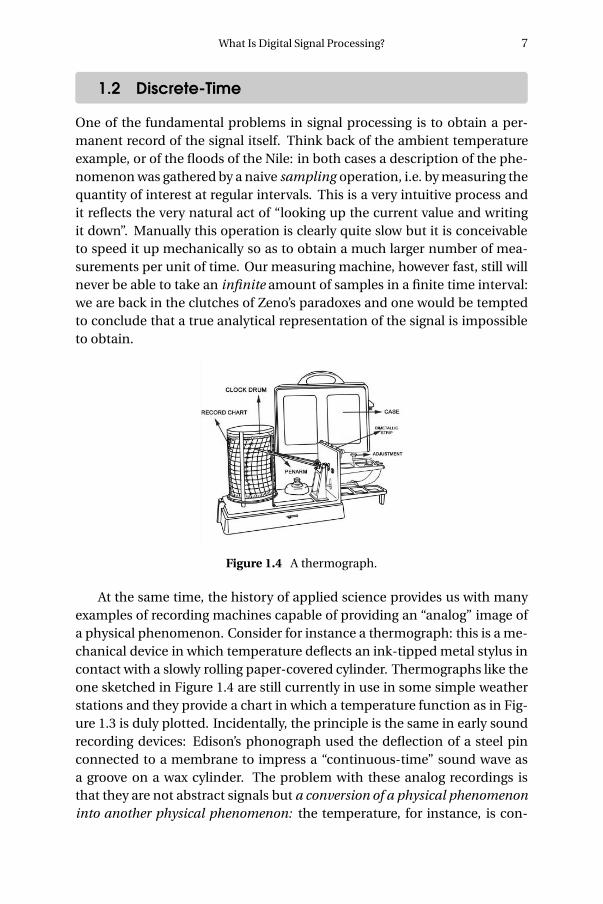
Figure 1.4 A thermograph.

At the same time, the history of applied science provides us with manyexamples of recording machines capable of providing an “analog” image ofa physical phenomenon. Consider for instance a thermograph: this is a me-chanical device in which temperature deflects an ink-tipped metal stylus incontact with a slowly rolling paper-covered cylinder. Thermographs like theone sketched in Figure 1.4 are still currently in use in some simple weatherstations and they provide a chart in which a temperature function as in Fig-ure 1.3 is duly plotted. Incidentally, the principle is the same in early soundrecording devices: Edison’s phonograph used the deflection of a steel pinconnected to a membrane to impress a “continuous-time” sound wave asa groove on a wax cylinder. The problem with these analog recordings isthat they are not abstract signals but a conversion of a physical phenomenoninto another physical phenomenon: the temperature, for instance, is con-

8 Discrete-Time

verted into the amount of ink on paper while the sound pressure wave isconverted into the physical depth of the groove. The advent of electron-ics did not change the concept: an audio tape, for instance, is obtained byconverting a pressure wave into an electrical current and then into a mag-netic deflection. The fundamental consequence is that, for analog signals,a different signal processing system needs to be designed explicitly for eachspecific form of recording.

T0 T1

� � � � ��

�

�

�

�

�

��

�

�

�

��

1 D

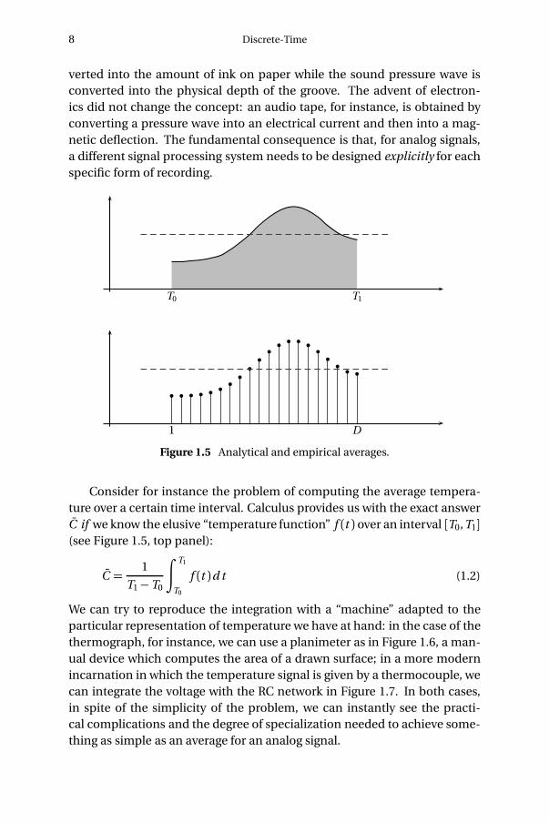
Figure 1.5 Analytical and empirical averages.

Consider for instance the problem of computing the average tempera-ture over a certain time interval. Calculus provides us with the exact answerC if we know the elusive “temperature function” f (t ) over an interval [T0,T1](see Figure 1.5, top panel):

C =1

T1−T0

∫ T1

T0

f (t )d t (1.2)

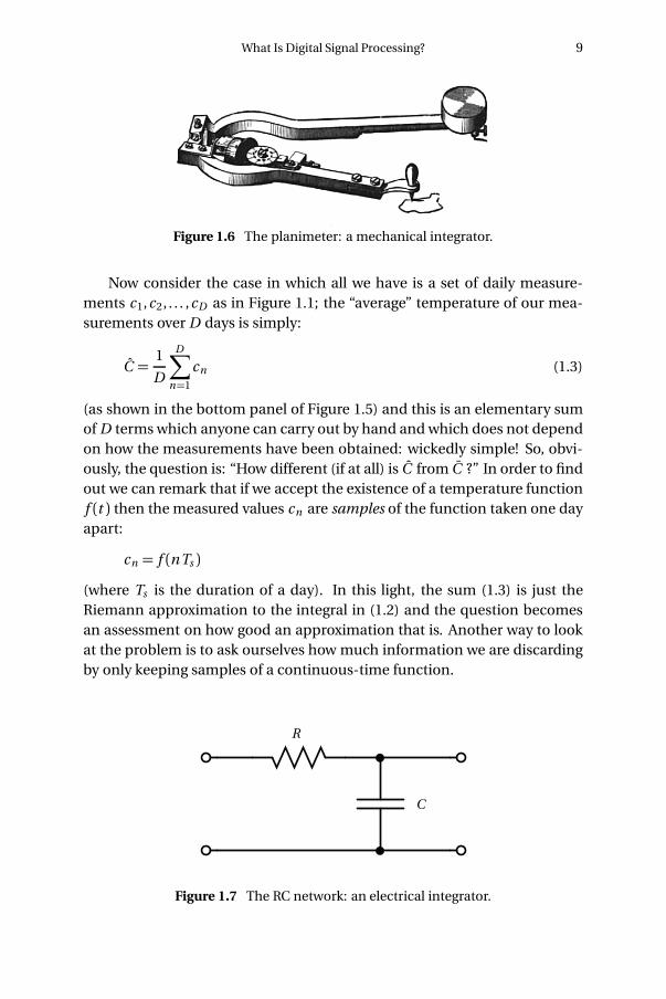
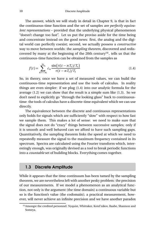
We can try to reproduce the integration with a “machine” adapted to theparticular representation of temperature we have at hand: in the case of thethermograph, for instance, we can use a planimeter as in Figure 1.6, a man-ual device which computes the area of a drawn surface; in a more modernincarnation in which the temperature signal is given by a thermocouple, wecan integrate the voltage with the RC network in Figure 1.7. In both cases,in spite of the simplicity of the problem, we can instantly see the practi-cal complications and the degree of specialization needed to achieve some-thing as simple as an average for an analog signal.


Figure 1.6 The planimeter: a mechanical integrator.

Now consider the case in which all we have is a set of daily measure-ments c1,c2, . . . ,cD as in Figure 1.1; the “average” temperature of our mea-surements over D days is simply:

C =1

D

D∑n=1

cn (1.3)

(as shown in the bottom panel of Figure 1.5) and this is an elementary sumof D terms which anyone can carry out by hand and which does not dependon how the measurements have been obtained: wickedly simple! So, obvi-ously, the question is: “How different (if at all) is C from C ?” In order to findout we can remark that if we accept the existence of a temperature functionf (t ) then the measured values cn are samples of the function taken one dayapart:

cn = f (nTs )

(where Ts is the duration of a day). In this light, the sum (1.3) is just theRiemann approximation to the integral in (1.2) and the question becomesan assessment on how good an approximation that is. Another way to lookat the problem is to ask ourselves how much information we are discardingby only keeping samples of a continuous-time function.

R

C

Figure 1.7 The RC network: an electrical integrator.

10 Discrete Amplitude

The answer, which we will study in detail in Chapter 9, is that in factthe continuous-time function and the set of samples are perfectly equiva-lent representations – provided that the underlying physical phenomenon“doesn’t change too fast”. Let us put the proviso aside for the time beingand concentrate instead on the good news: first, the analog and the digi-tal world can perfectly coexist; second, we actually possess a constructiveway to move between worlds: the sampling theorem, discovered and redis-covered by many at the beginning of the 20th century(4), tells us that thecontinuous-time function can be obtained from the samples as

f (t ) =∞∑

n=−∞cn

sin�π(t −nTs )/Ts

�π(t −nTs )/Ts

(1.4)

So, in theory, once we have a set of measured values, we can build thecontinuous-time representation and use the tools of calculus. In realitythings are even simpler: if we plug (1.4) into our analytic formula for theaverage (1.2) we can show that the result is a simple sum like (1.3). So wedon’t need to explicitly go “through the looking glass” back to continuous-time: the tools of calculus have a discrete-time equivalent which we can usedirectly.

The equivalence between the discrete and continuous representationsonly holds for signals which are sufficiently “slow” with respect to how fastwe sample them. This makes a lot of sense: we need to make sure thatthe signal does not do “crazy” things between successive samples; only ifit is smooth and well behaved can we afford to have such sampling gaps.Quantitatively, the sampling theorem links the speed at which we need torepeatedly measure the signal to the maximum frequency contained in itsspectrum. Spectra are calculated using the Fourier transform which, inter-estingly enough, was originally devised as a tool to break periodic functionsinto a countable set of building blocks. Everything comes together.

1.3 Discrete Amplitude

While it appears that the time continuum has been tamed by the samplingtheorem, we are nevertheless left with another pesky problem: the precisionof our measurements. If we model a phenomenon as an analytical func-tion, not only is the argument (the time domain) a continuous variable butso is the function’s value (the codomain); a practical measurement, how-ever, will never achieve an infinite precision and we have another paradox

(4)Amongst the credited personnel: Nyquist, Whittaker, Kotel’nikov, Raabe, Shannon andSomeya.


on our hands. Consider our temperature example once more: we can usea mercury thermometer and decide to write down just the number of de-grees; maybe we can be more precise and note the half-degrees as well; witha magnifying glass we could try to record the tenths of a degree – but wewould most likely have to stop there. With a more sophisticated thermo-couple we could reach a precision of one hundredth of a degree and possiblymore but, still, we would have to settle on a maximum number of decimalplaces. Now, if we know that our measures have a fixed number of digits,the set of all possible measures is actually countable and we have effectivelymapped the codomain of our temperature function onto the set of integernumbers. This process is called quantization and it is the method, togetherwith sampling, to obtain a fully digital signal.

In a way, quantization deals with the problem of the continuum in amuch “rougher” way than in the case of time: we simply accept a loss ofprecision with respect to the ideal model. There is a very good reason forthat and it goes under the name of noise. The mechanical recording deviceswe just saw, such as the thermograph or the phonograph, give the illusionof analytical precision but are in practice subject to severe mechanical lim-itations. Any analog recording device suffers from the same fate and evenif electronic circuits can achieve an excellent performance, in the limit theunavoidable thermal agitation in the components constitutes a noise floorwhich limits the “equivalent number of digits”. Noise is a fact of nature thatcannot be eliminated, hence our acceptance of a finite (i.e. countable) pre-cision.

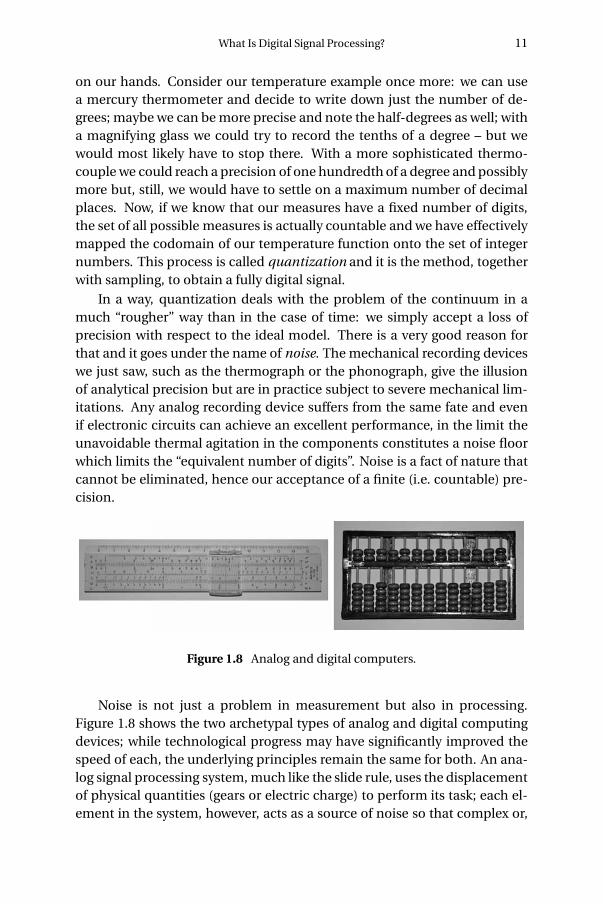
Figure 1.8 Analog and digital computers.

Noise is not just a problem in measurement but also in processing.Figure 1.8 shows the two archetypal types of analog and digital computingdevices; while technological progress may have significantly improved thespeed of each, the underlying principles remain the same for both. An ana-log signal processing system, much like the slide rule, uses the displacementof physical quantities (gears or electric charge) to perform its task; each el-ement in the system, however, acts as a source of noise so that complex or,

12 Communication Systems

more importantly, cheap designs introduce imprecisions in the final result(good slide rules used to be very expensive). On the other hand the aba-cus, working only with integer arithmetic, is a perfectly precise machine(5)

even if it’s made with rocks and sticks. Digital signal processing works withcountable sequences of integers so that in a digital architecture no process-ing noise is introduced. A classic example is the problem of reproducing asignal. Before mp3 existed and file sharing became the bootlegging methodof choice, people would “make tapes”. When someone bought a vinyl recordhe would allow his friends to record it on a cassette; however, a “peer-to-peer” dissemination of illegally taped music never really took off because ofthe “second generation noise”, i.e. because of the ever increasing hiss thatwould appear in a tape made from another tape. Basically only first genera-tion copies of the purchased vinyl were acceptable quality on home equip-ment. With digital formats, on the other hand, duplication is really equiva-lent to copying down a (very long) list of integers and even very cheap equip-ment can do that without error.

Finally, a short remark on terminology. The amplitude accuracy of a setof samples is entirely dependent on the processing hardware; in currentparlance this is indicated by the number of bits per sample of a given rep-resentation: compact disks, for instance, use 16 bits per sample while DVDsuse 24. Because of its “contingent” nature, quantization is almost always ig-nored in the core theory of signal processing and all derivations are carriedout as if the samples were real numbers; therefore, in order to be precise,we will almost always use the term discrete-time signal processing and leavethe label “digital signal processing” (DSP) to the world of actual devices. Ne-glecting quantization will allow us to obtain very general results but caremust be exercised: in the practice, actual implementations will have to dealwith the effects of finite precision, sometimes with very disruptive conse-quences.

1.4 Communication Systems

Signals in digital form provide us with a very convenient abstract represen-tation which is both simple and powerful; yet this does not shield us fromthe need to deal with an “outside” world which is probably best modeled bythe analog paradigm. Consider a mundane act such as placing a call on acell phone, as in Figure 1.9: humans are analog devices after all and theyproduce analog sound waves; the phone converts these into digital format,

(5)As long as we don’t need to compute square roots; luckily, linear systems (which is whatinterests us) are made up only of sums and multiplications.


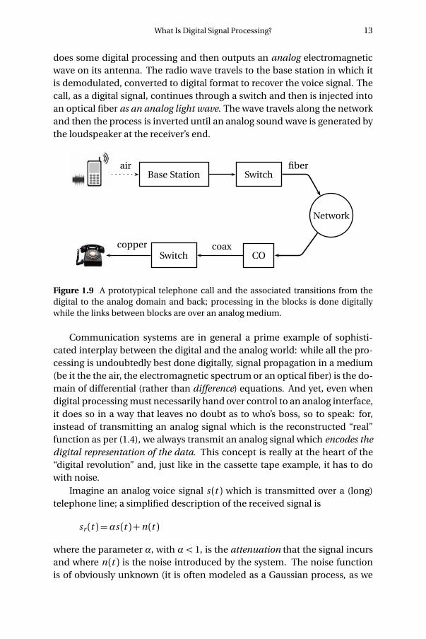
does some digital processing and then outputs an analog electromagneticwave on its antenna. The radio wave travels to the base station in which itis demodulated, converted to digital format to recover the voice signal. Thecall, as a digital signal, continues through a switch and then is injected intoan optical fiber as an analog light wave. The wave travels along the networkand then the process is inverted until an analog sound wave is generated bythe loudspeaker at the receiver’s end.

Base Station Switch

Network

Switch CO

air

coaxcopper

fiber

Figure 1.9 A prototypical telephone call and the associated transitions from thedigital to the analog domain and back; processing in the blocks is done digitallywhile the links between blocks are over an analog medium.

Communication systems are in general a prime example of sophisti-cated interplay between the digital and the analog world: while all the pro-cessing is undoubtedly best done digitally, signal propagation in a medium(be it the the air, the electromagnetic spectrum or an optical fiber) is the do-main of differential (rather than difference) equations. And yet, even whendigital processing must necessarily hand over control to an analog interface,it does so in a way that leaves no doubt as to who’s boss, so to speak: for,instead of transmitting an analog signal which is the reconstructed “real”function as per (1.4), we always transmit an analog signal which encodes thedigital representation of the data. This concept is really at the heart of the“digital revolution” and, just like in the cassette tape example, it has to dowith noise.

Imagine an analog voice signal s (t ) which is transmitted over a (long)telephone line; a simplified description of the received signal is

sr (t ) =αs (t )+n (t )

where the parameter α, with α < 1, is the attenuation that the signal incursand where n (t ) is the noise introduced by the system. The noise functionis of obviously unknown (it is often modeled as a Gaussian process, as we


will see) and so, once it’s added to the signal, it’s impossible to eliminate it.Because of attenuation, the receiver will include an amplifier with gain G torestore the voice signal to its original level; with G = 1/α we will have

sa (t ) =G sr (t ) = s (t )+G n (t )

Unfortunately, as it appears, in order to regenerate the analog signal we alsohave amplified the noise G times; clearly, if G is large (i.e. if there is a lot ofattenuation to compensate for) the voice signal end up buried in noise. Theproblem is exacerbated if many intermediate amplifiers have to be used incascade, as is the case in long submarine cables.

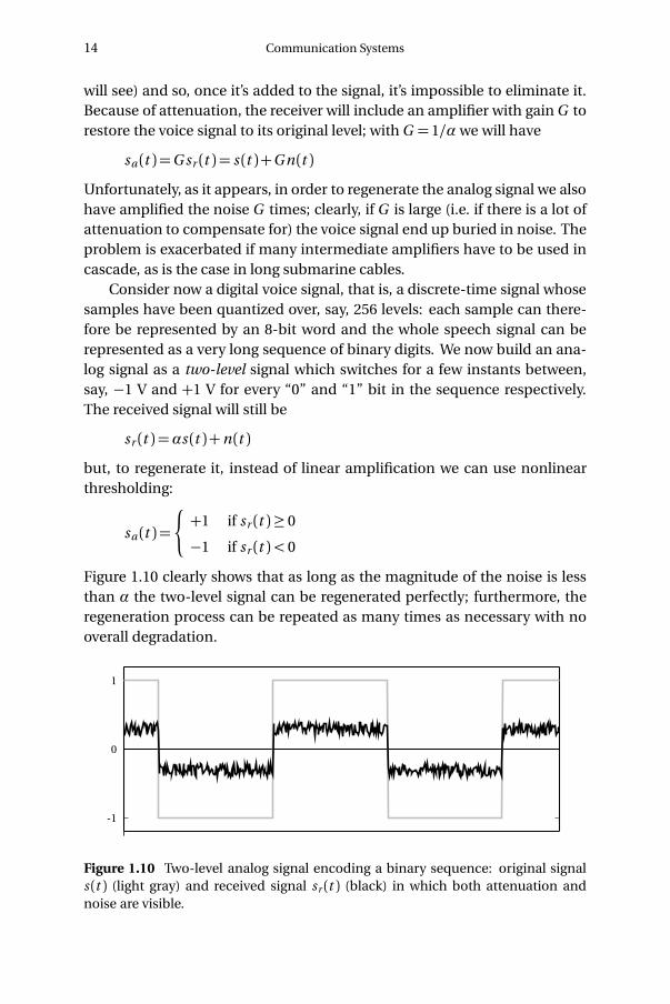
Consider now a digital voice signal, that is, a discrete-time signal whosesamples have been quantized over, say, 256 levels: each sample can there-fore be represented by an 8-bit word and the whole speech signal can berepresented as a very long sequence of binary digits. We now build an ana-log signal as a two-level signal which switches for a few instants between,say, −1 V and +1 V for every “0” and “1” bit in the sequence respectively.The received signal will still be

sr (t ) =αs (t )+n (t )

but, to regenerate it, instead of linear amplification we can use nonlinearthresholding:

sa (t ) =

�+1 if sr (t )≥ 0

−1 if sr (t )< 0

Figure 1.10 clearly shows that as long as the magnitude of the noise is lessthan α the two-level signal can be regenerated perfectly; furthermore, theregeneration process can be repeated as many times as necessary with nooverall degradation.

0

1

-1

Figure 1.10 Two-level analog signal encoding a binary sequence: original signals (t ) (light gray) and received signal sr (t ) (black) in which both attenuation andnoise are visible.


In reality of course things are a little more complicated and, because ofthe nature of noise, it is impossible to guarantee that some of the bits won’tbe corrupted. The answer is to use error correcting codes which, by introduc-ing redundancy in the signal, make the sequence of ones and zeros robustto the presence of errors; a scratched CD can still play flawlessly because ofthe Reed-Solomon error correcting codes used for the data. Data coding isthe core subject of Information Theory and it is behind the stellar perfor-mance of modern communication systems; interestingly enough, the mostsuccessful codes have emerged from group theory, a branch of mathemat-ics dealing with the properties of closed sets of integer numbers. Integersagain! Digital signal processing and information theory have been able tojoin forces so successfully because they share a common data model (the in-teger) and therefore they share the same architecture (the processor). Com-puter code written to implement a digital filter can dovetail seamlessly withcode written to implement error correction; linear processing and nonlinearflow control coexist naturally.

A simple example of the power unleashed by digital signal processingis the performance of transatlantic cables. The first operational telegraphcable from Europe to North America was laid in 1858 (see Fig. 1.11); itworked for about a month before being irrecoverably damaged.(6) Fromthen on, new materials and rapid progress in electrotechnics boosted theperformance of each subsequent cable; the key events in the timeline oftransatlantic communications are shown in Table 1.1. The first transatlantictelephone cable was laid in 1956 and more followed in the next two decadeswith increasing capacity due to multicore cables and better repeaters; theinvention of the echo canceler further improved the number of voice chan-nels for already deployed cables. In 1968 the first experiments in PCM digitaltelephony were successfully completed and the quantum leap was aroundthe corner: by the end of the 70’s cables were carrying over one order ofmagnitude more voice channels than in the 60’s. Finally, the deployment ofthe first fiber optic cable in 1988 opened the door to staggering capacities(and enabled the dramatic growth of the Internet).

Finally, it’s impossible not to mention the advent of data compressionin this brief review of communication landmarks. Again, digital processingallows the coexistence of standard processing with sophisticated decision

(6)Ohm’s law was published in 1861, so the first transatlantic cable was a little bit theproverbial cart before the horse. Indeed, the cable circuit formed an enormous RCequivalent circuit, i.e. a big lowpass filter, so that the sharp rising edges of the Morsesymbols were completely smeared in time. The resulting intersymbol interference wasso severe that it took hours to reliably send even a simple sentence. Not knowing howto deal with the problem, the operator tried to increase the signaling voltage (“crank upthe volume”) until, at 4000 V, the cable gave up.


Figure 1.11 Laying the first transatlantic cable.

Table 1.1 The main transatlantic cables from 1858 to our day.

Cable Year Type Signaling Capacity

1858 Coax telegraph a few words per hour

1866 Coax telegraph 6-8 words per minute

1928 Coax telegraph 2500 characters per minute

TAT-1 1956 Coax telephone 36 [48 by 1978] voice channels



TAT-6 1976 Coax telephone 4000 [10, 000 by 1994] voice channels

TAT-8 1988 Fiber data 280 Mbit/s (∼ 40, 000 voice channels)

TAT-14 2000 Fiber data 640 Gbit/s (∼ 9, 700, 000 voice channels)

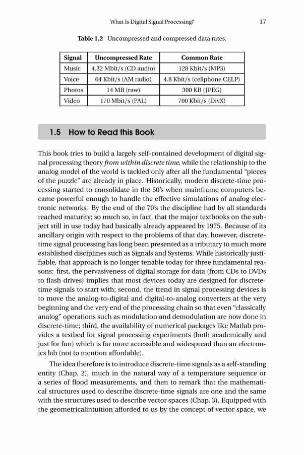
logic; this enables the implementation of complex data-dependent com-pression techniques and the inclusion of psychoperceptual models in orderto match the compression strategy to the characteristics of the human vi-sual or auditory system. A music format such as mp3 is perhaps the firstexample to come to mind but, as shown in Table 1.2, all communication do-mains have been greatly enhanced by the gains in throughput enabled bydata compression.


Table 1.2 Uncompressed and compressed data rates.

Signal Uncompressed Rate Common Rate

Music 4.32 Mbit/s (CD audio) 128 Kbit/s (MP3)

Voice 64 Kbit/s (AM radio) 4.8 Kbit/s (cellphone CELP)

Photos 14 MB (raw) 300 KB (JPEG)

Video 170 Mbit/s (PAL) 700 Kbit/s (DivX)

1.5 How to Read this Book

This book tries to build a largely self-contained development of digital sig-nal processing theory from within discrete time, while the relationship to theanalog model of the world is tackled only after all the fundamental “piecesof the puzzle” are already in place. Historically, modern discrete-time pro-cessing started to consolidate in the 50’s when mainframe computers be-came powerful enough to handle the effective simulations of analog elec-tronic networks. By the end of the 70’s the discipline had by all standardsreached maturity; so much so, in fact, that the major textbooks on the sub-ject still in use today had basically already appeared by 1975. Because of itsancillary origin with respect to the problems of that day, however, discrete-time signal processing has long been presented as a tributary to much moreestablished disciplines such as Signals and Systems. While historically justi-fiable, that approach is no longer tenable today for three fundamental rea-sons: first, the pervasiveness of digital storage for data (from CDs to DVDsto flash drives) implies that most devices today are designed for discrete-time signals to start with; second, the trend in signal processing devices isto move the analog-to-digital and digital-to-analog converters at the verybeginning and the very end of the processing chain so that even “classicallyanalog” operations such as modulation and demodulation are now done indiscrete-time; third, the availability of numerical packages like Matlab pro-vides a testbed for signal processing experiments (both academically andjust for fun) which is far more accessible and widespread than an electron-ics lab (not to mention affordable).

The idea therefore is to introduce discrete-time signals as a self-standingentity (Chap. 2), much in the natural way of a temperature sequence ora series of flood measurements, and then to remark that the mathemati-cal structures used to describe discrete-time signals are one and the samewith the structures used to describe vector spaces (Chap. 3). Equipped withthe geometricalintuition afforded to us by the concept of vector space, we

18 Further Reading

can proceed to “dissect” discrete-time signals with the Fourier transform,which turns out to be just a change of basis (Chap. 4). The Fourier trans-form opens the passage between the time domain and the frequency do-main and, thanks to this dual understanding, we are ready to tackle theconcept of processing as performed by discrete-time linear systems, alsoknown as filters (Chap. 5). Next comes the very practical task of designinga filter to order, with an eye to the subtleties involved in filter implementa-tion; we will mostly consider FIR filters, which are unique to discrete time(Chaps 6 and 7). After a brief excursion in the realm of stochastic sequences(Chap. 8) we will finally build a bridge between our discrete-time world andthe continuous-time models of physics and electronics with the concepts ofsampling and interpolation (Chap. 9); and digital signals will be completelyaccounted for after a study of quantization (Chap. 10). We will finally goback to purely discrete time for the final topic, multirate signal processing(Chap. 11), before putting it all together in the final chapter: the analysis ofa commercial voiceband modem (Chap. 12).

Further Reading

The Bible of digital signal processing was and remains Discrete-Time Sig-nal Processing, by A. V. Oppenheim and R. W. Schafer (Prentice-Hall, lastedition in 1999); exceedingly exhaustive, it is a must-have reference. Forbackground in signals and systems, the eponimous Signals and Systems, byOppenheim, Willsky and Nawab (Prentice Hall, 1997) is a good start.

Most of the historical references mentioned in this introduction can beintegrated by simple web searches. Other comprehensive books on digi-tal signal processing include S. K. Mitra’s Digital Signal Processing (McGrawHill, 2006) and Digital Signal Processing, by J. G. Proakis and D. K. Manolakis(Prentis Hall 2006). For a fascinating excursus on the origin of calculus, seeD. Hairer and G. Wanner, Analysis by its History (Springer-Verlag, 1996). Amore than compelling epistemological essay on the continuum is Every-thing and More, by David Foster Wallace (Norton, 2003), which manages tobe both profound and hilarious in an unprecedented way.

Finally, the very prolific literature on current signal processing researchis published mainly by the Institute of Electronics and Electrical Engineers(IEEE) in several of its transactions such as IEEE Transactions on Signal Pro-cessing, IEEE Transactions on Image Processing and IEEE Transactions onSpeech and Audio Processing.

what is digital signal processing? · 2008-08-28 · digital signal processing is aﬂavor of...

Documents