1

Welfare consistent tariff aggregators at different geographical resolutions: a bilateral perspective

Mihaly Himics*†, Wolfgang Britz†

*corresponding author

†Institute for Food and Resource Economics, University of Bonn

Address: Nussallee 21, 53115 Bonn, Germany Email addresses: mihaly.himics@ilr.uni-bonn.de (M. Himics), wolfgang.britz@ilr.uni-bonn.de (W. Britz)

Abstract

In this paper we develop a technique to aggregate tariffs on imports from heterogeneous trade blocs in a

welfare consistent manner. The technique enables a welfare consistent analysis of free trade

agreements (FTA) in the general equilibrium framework regardless the geographical resolution of

exporter countries. Explicitly addressing the regional dimension in the tariff aggregation problem has

been made important by the increased use of flexible regional aggregation techniques in applied

modeling in the last decade, largely facilitated by dedicated software tools and databases.

The flexible aggregation of countries in applied trade models requires an approach to aggregate tariffs

and other border protection measures. Most widely used approaches, however, are based on trade

weighted averages that are not grounded in economic theory. The lack of theoretical consistency results

in underestimated tariff protection and delivers inconsistent simulated welfare effects at the higher level

of geographical aggregation. Suitable techniques for welfare consistent tariff aggregation in the general

equilibrium framework have been developed by Bach and Martin (2001) and Anderson (2009). We

further extend their original approach in the context of flexible regional aggregation by including an

explicit regional dimension for imports and by including tariff rate quotas (TRQ), an important trade

policy instrument, especially in agricultural and food markets. The extended approach allows for flexible

and welfare consistent aggregation of tariffs and TRQs, regardless of the geographical resolution of the

exporter trade blocs.

Both a didactic example and an assessment of the Korean dairy market in the EU-South Korea FTA

illustrate how the tariff aggregators can be derived and incorporated in applied equilibrium models. Our

results suggest that the simulated gains from trade liberalization are underestimated by traditional trade

weighted tariff aggregators. This is not only true in the context of unilateral trade liberalization (as has

been already pointed out by many authors in the literature), but also for bi- and multilateral trade

agreements. The use of dedicated, welfare consistent tariff aggregators thus seems to be inevitable in ex

ante evaluations of FTAs if welfare implications are to be analyzed.

2

1 Introduction Aggregation of trade flows and tariffs is inevitable in empirical models of international trade. Although

trade statistics (data on trade flows and trade policy instruments) are usually available at the fine level of

tariff lines (Guimbard et al. 2012), this is unfortunately no the case with respect to other items of

commodity balances (supply, consumption etc.). That discrepancy between nomenclatures of trade

statistics and other data sources lead to a multitude of tariff aggregation methods in applied equilibrium

models (AEM). The still widely used conventional trade weighted average tariffs are however not

grounded in economic theory and suffer from the endogeneity bias as higher tariffs decrease imports

and thus aggregation weights. As a result, they systematically underestimate tariff protection at

aggregate level, cf. Pelikan and Brockmeier (2008).

Anderson and Neary (1994) pioneered the field of consistent tariff aggregation by defining index

measures of tariffs that are consistent with selected economic indicators (e.g. welfare). They base e.g.

their Trade Restrictiveness Index (TRI) on a compensating variation measure of welfare changes defined

over the country’s balance of trade (Martin 1997). The TRI can be converted into a uniform ad valorem

tariff rate that implies the same welfare changes in the economy as the individual tariff rates would do.

Unfortunately, one single index number (such as the TRI) does not suffice in the general equilibrium

framework. The different marginal impact of tariff reduction on tariff revenues and expenditures creates

a tension in the balance of trade that cannot be resolved with one single tariff aggregator. Bach and

Martin (2001) first overcome the issue by defining different aggregators for the expenditure function and

for the tariff revenue function. Their approach, however, requires a complete general equilibrium model

at the tariff line to aggregate over the tariff revenues. With several thousand tariff lines in a typical tariff

schedule of an FTA, this requirement imposes a serious computational burden. Anderson (2009) reduces

significantly the computational efforts needed for consistent aggregation when building his method on

two tariff aggregators that can be computed without a full-fledged model at the tariff line. He plugs in an

optimal combination of a trade weighted aggregator and what he calls the 'true average tariff' (TAT) into

the trade balance condition. That optimal tariff combination can be derived pre-model, in aggregation

modules only loosely linked to AEMs, as demonstrated by Laborde et al. (2011). Section 2.1 provides a

review of that strand of literature.

Other approaches circumvent the tariff aggregation problem by shifting trade policies into model

extensions working at the tariff line level. (Grant et al. 2007) develop a satellite partial equilibrium (PE)

model of the global dairy markets at the tariff line level and link it iteratively to the general equilibrium

(GE) structure of Global Trade Analysis Project (GTAP) model (T. W. Hertel 1999). Also in the GTAP

framework, (Narayanan et al. 2010) investigates the impact of tariff liberalization on the Indian auto

industry with a nested PE-GE approach. Both approaches successfully avoid aggregating tariffs directly,

and in theory they provide an alternative to welfare consistent tariff aggregators. Unfortunately, neither

the nested PE-GE approach nor the iterative model link scale up well: extending the approaches to all

commodity markets or industries covered by the aggregate model generates numerical problems.

Therefore tariff aggregation remains unavoidable in applied policy modeling.

3

This paper adapts the Anderson framework for AEMs analyzing preferential and regional trade

agreements, taking advantage of flexible regional aggregation (see section 2.2). This bilateral aspect is a

key contribution of the paper, in contrast to previous applications in the literature that focused on

overall trade restrictiveness in the face of unilateral trade liberalization (Anderson 2009) or on

multilateral trade liberalization (Bureau and Salvatici 2004, Manole and Martin 2005 or Laborde et al.

2011). The extended approach is also suitable for flexible regional aggregation of e.g. tariff databases or

tariffs in Social Accounting Matrices. It is therefore a welfare consistent tariff aggregation alternative to

software tools such as GTAPAgg (Horridge 2008) or the popular tariff aggregation tool TASTE (Horridge

and Laborde 2008) that apply trade weighted averages and thus might deliver inconsistent welfare

results.

A further contribution of the paper is the inclusion of TRQs in the Anderson tariff aggregation

framework. Despite that fact that Anderson (2009) already discussed the techniques to handle import

quotas, his optimal combination of tariff aggregators has not yet been adapted in the literature to a case

where TRQs are explicitly modeled. Section 2.3 demonstrates how to include the per unit quota rent via

a shadow tariff in the aggregation framework, using a Mixed Complementarity Problem (Rutherford

1995) approach. Welfare consistent tariff aggregators covering bi-lateral TRQs then can be defined and

combined with those in the Anderson’s original approach in a natural way.

The technique is presented in two empirical applications. One of them is the same didactic example as in

Bach and Martin (2001, page 630-632) in order to make a direct comparison of the techniques possible.

In section 3.2 our extended approach is applied to the impact assessment of the EU-South Korea Free

Trade Agreement (FTA) on the Korean dairy market. Different (conventional and welfare consistent)

tariff aggregators are estimated and compared for the Korean dairy imports from the EU at different

stages of the FTA implementation and at different geographical resolutions for the EU. The estimates are

specific to the main European exporter countries of dairy products to Korea while taking into account the

several TRQ mechanisms operating on the market. Section 4 concludes with a short summary and with

some general remarks on using consistent tariff aggregators in applied modeling work.

2 Methodology for consistent aggregators of trade policies

2.1 Standard welfare-consistent aggregators This section is a formal introduction to the welfare consistent tariff aggregators for the general

equilibrium framework. In section 3 the tariff aggregators are illustrated with a numerical example. Bach

and Martin (2001) first called attention to the problem of welfare consistent tariff aggregation in the

general equilibrium. The discussion below, however, builds mostly on the subsequent work on Anderson

(2009), using his notations and terms, and refers back to the original Bach-Martin approach only to

highlight differences.

The tariff aggregation techniques presented here aim at deriving uniform tariffs that are optimal in the

sense that when substituted into an underlying objective function they yield the same result as the non-

uniform tariff structure would do. Structure, parameterization and input data of the underlying model all

have an impact on the derived aggregated tariffs.

4

Let us consider a small open economy, where a subset of tradable goods is to be aggregated. The vector

of domestic prices is partitioned to ( , ),p where p denotes the price vector of products to be

aggregated and denotes the prices of other tradables. Trade policies1 wedge domestic prices away

from constant world prices ( , ).w wp First a trade balance equilibrium condition is constructed for the

economy, based on the international budget constraint. That condition is formulated based on a trade

expenditure function, defined as the difference between the consumers’ expenditure function and the

gross domestic product (GDP) function:

, ) ( , , ) (, , )(E e pp u u g p

where u denotes real income. The excess demand functions can be derived by the Shephard and

Hotelling Lemmas respectively: p p pE e g and E e g (the subscripts denote partial

derivatives).

The balance of trade condition then guarantees that the value of imports is equal to the value of exports

plus a possible financial inflow :b

, , , ) (( , , ) ( , ) ( ) 0.w w w w

pB p E p E Eu p u p p b (1)

By reclassifying the real income as exogenous, i.e. fixing real GDP, the function B above (termed the

balance of trade function) provides a compensation measure of welfare changes (Martin 1997). The TRI

index (Anderson and Neary 2005) is based exactly on this welfare measure. The TRI uniform tariff factor,

denoted by 1 , is the tariff rate that would aggregate the single tariffs without altering the balance

of trade:

) ,: ((1 , , , ) ( , , , ).,w w w w wB p u p B p u p

Consistent aggregation with regard to the balance of trade function requires further restrictions both on

the supply and demand sides of the economy. We assume (weakly) separable demand for the product

group with price vector p and assume that the group enters consumer preferences homothetically.

Separable homotheticity implies two-stage budgeting and allows to define price indexes over product

groups entering the top level of the consumers’ budget allocation problem (Deaton and Muellbauer

1980).

Consistent aggregation does not allow for relative price changes on the supply side in the commodity

group being aggregated. A sufficient condition to avoid relative price changes is that supply prices (the

world price vector wp ) are independent of trade policies. That condition is automatically satisfied in the

small country case due to the fix world prices. A Ricardian economy, where countries are specialized in

either exporting or importing certain goods but never in both, enables consistent aggregation too.

Supply prices are not affected by import tariffs in a Ricardian economy and so tariff aggregation does not

1 For the sake of simplicity, we only consider tariffs as a cause for the price wedges in this theoretical discussion.

Accordingly, we refer to the aggregation of trade policy instruments as tariff aggregation.

5

change relative supply prices. Even weaker supply side separability assumptions can make consistent

aggregation possible, as discussed by Anderson (2009).

While the TRI index reproduces the balance of trade, it cannot get both the trade volumes and the tariff

revenues right (Anderson 2009). The solution suggested by Bach and Martin (2001) is to use two

different aggregators in the different terms of equation (1): one for the trade expenditure and one for

the tariff revenue part. Taking advantage of separable homotheticity, we can construct an aggregator for

the expenditure part as an implicit function of the domestic price vector:

,: | ( ( ), , , ) ( , , , ).,n w w w wE p u p E p u p (2)

The 'true average tariff' (Anderson 2009) can then be introduced as:

(.

)1

)

(

wpT

p

(3)

Under specific restrictions, it is possible to derive a closed-form solution for T (see Manole and Martin

2005). Here we focus on setting up a modeling framework to numerically derive the tariff aggregators,

and so for our purposes the above implicit formula is satisfactory.

Following Anderson, we define the second aggregator, for the tariff revenue part, as a combination of

T and the simple trade weighted average tariff. The trade weighted average tariff is calculated as:

,j

a

j jT w T (4)

where the index j runs over the imported goods with price vector ,p / ( )j jj p pj jj

w p E p E

denote value shares and ( ) /j j

w

j jT p p p are the single tariff rates relative to the domestic prices.

The expression for tariff revenues then can be substituted2 with an optimal combination of ( , )aT T in

equation (1):

( ) ( )

( , ( ) 0) .1 1

,w w

a wpE E E b

T T

pu T

(5)

The above aggregation is consistent with respect to the domestic expenditure on imports (by definition,

see the first term) and also guarantees that the aggregation does not alter welfare (the balance of trade

remains unchanged). Obviously, that also implies consistency with respect to tariff revenues, as they are

simply the difference between the trade balance and trade expenditures.

2.2 Introducing a regional dimension for the tariff aggregators In the following section we introduce an explicit regional dimension in the above framework by splitting

up the exporter country into sub-regions. As a result, imported goods are differentiated both by tariff

2 For a formal derivation of the formula see Appendix A

6

line and by place of origin. First we define sub-region-specific aggregator functions analogue to equation

(2):

1 1( , ): | (( ( )) , ( ,, , ) , ),n m n

n i

n

iE p u uE p

(6)

where the i subscript runs over the exporter regions and the number of imported product types

(number of tariff lines) is .m Exporter specific versions of the ‘true average tariff’ rates can then simply

be calculated as:

( )

{1, , }.(

1 ,)

w

ii

i

piT n

p

(7)

Unfortunately, there are more variables than equations in the equation system of (6) and thus a unique

solution to the problem does not exist, in general. In the separable homothetic case, however, equation

(6) reduces to a problem where the aggregators are calculated based on their impact on the composite

price index:

1 1( , ): | ((, ( )) , () ),,n m n

n c i c

n

i pp p p

(8)

simply because in this case , , ,, )( ) (cu pE pp u where cp denotes the composite price index.

In particular, it is possible to derive the regional aggregators for each region independently:

1( , ( ), ) ), {1, ,, ): | ( , ( },,n m n i

n c i cp pp p p i n (9)

where ip denotes domestic prices of all imported commodities other than exported by region .i A

formal proof for the equivalence of 1( )i

n

i and 1( )i

n

i is provided in Appendix A.

The second aggregator for the trade weighted averages only needs to be extended with an additional

regional dimension in order to arrive at exporter specific ones:

1

, , {1, , },,m

i j i j

a

i

j

iT w T n

where j runs over the index set of commodities. The single tariff rates relative to the domestic prices are

calculated as ,, , ,( ) / ,i j i j i i

w

j jT p p p and the value shares take the form:

,

,

.

,

,

, .,i j

i j

i j p

i j

i

j

j p

p Ew

p Ei j

7

Using the inherited homogeneity property of 1 ), (i i n the optimal combination of ( , )aT T

can be broken down3 to a sum of regional combinations 1( :, )a n

i i iT T

.1 1

( )( )i

wa

i

i i

wa iT E T E

T T

pp

The above expression leads to the regional version of the balance of trade condition:

1

1

( ) (, , ( ) 0.

1

)( ), ,

1 1i

w wwwian

i

in i

E T E E bT T

ppu

T

p

2.3 Consistent aggregators for tariffs under TRQ Tariff rate quotas (TRQ) are two-tiered tariff instruments where a lower (preferential) tariff rate is

applied on imports until a pre-defined quota threshold is reached. Imports exceeding the quota level are

subject to a higher, typically the Most Favored Nation (MFN), tariff rate. Many TRQs were introduced in

the Uruguay Round of negotiations during the tariffication process, both to provide a minimum market

access to highly protected markets and to maintain pre-existing trade preferences. Although the number

of tariff lines protected by TRQs has been decreasing in the last decade, they are still crucial border

protection measures for agricultural trade (World Trade Organization 2012). Additionally, TRQs are often

introduced in the context of FTAs, at least during an intermediate implementation period.

The world trade of dairy products is traditionally complicated by TRQ regimes, and therefore the

inclusion of TRQs in the above model structure is of practical relevance in the empirical section of this

paper. The formal discussion below extends Anderson’s treatment (2009, Appendix A) of import quotas

to the TRQ case. The implementation consists of two main elements: (1) a price mechanism that defines

the tariff inclusive domestic prices depending on the relations between fill rate, excess demand and

supply and (2) an assumption on how the quota rent is allocated between the home country and the

exporters (the so-called quota allocation share). The rent allocation primarily depends on the quota

administration method (Boughner et al. 2000). The WTO currently gives freedom to their members to

choose the administration method and therefore a wide variety of effective quota allocation shares are

possible.

Let assume that there exist rent retaining tariff rates ( ) for all tariff lines and that a given percentage

( )s of the rent above that tariff rate goes to foreign countries; the rest (1 )s being attributed to the

home country. The per unit quota rent retained at home then can be calculated as:

(1 )( ) (1 ) )( .w ws p p s s p p

Quota rents allocated to the importer country appear in the balance of trade as lump sum transfers to

consumers and only accrue if the quota is filled. Above the threshold normal tariff revenues are collected

3 For a formal proof consult Appendix B

8

at the MFN rate. Partitioning the excess demand into in-quota and out-of-quota imports ( , )in out

p ppE E E

, the balance of trade condition takes the form:

, ) (1( , , ) ) () 0( ( ) .w in w out w

p pu s s p p EE p q Ep bp E

Our aim of substituting the TRQ mechanisms at the tariff line with an aggregate equivalent tariff rate

does not allow for the above partitioning of pE in the aggregate balance of trade condition. Therefore,

we opt for an alternative formulation and first calculate the quota rent for the entire import volume

followed by a correction on the out-of-quota imports. The correction term is calculated based on the

difference between the MFN rate and the unit quota rent retained at home:

( ) (1 )( ) ( .)w w wp p s p p s p p s

Plugging it in the balance of trade yields:

, ) (( , , )1

) ( ) ( ) 0,

)(

(

w q

p

w out w

p

u s s p p E

s p

E p q I

s q Ep E I b

(10)

where q denotes the vector of quota thresholds. outI and

qI are vectors at the tariff line level indicating

whether quotas are overfilled such that a correction on out-of-quota imports is needed, respectively

quotas filled such that quota rents occur.

The domestic price p above is derived from a model-endogenous price mechanism. Following a popular

approach, the TRQ regimes in our modeling framework are represented by orthogonality constraints in

an MCP framework (see e.g. Junker and Heckelei 2012).

In order to reach an aggregate form of equation (10), additional terms need to be introduced. The

aggregator for the rent retaining tariff rates is defined as:

,j

R R

j jT w T

where iw are value shares and / .R

j j j jT s p

In order to calculate the effective tariff content, the trade weighted average tariff must be adjusted with

the rent allocation shares :s

(1 )

.ˆ ˆ ˆ: where a j in

j j j j j

j j

sT w T T E

pq

Similarly, we introduce two tariff aggregators for the out-of-quota correction term in equation (10):

9

,( )

ˆ ˆ ˆ: , whe e 0r

w

j j jcorr corr out

j j j j

j j

a corrs p p

T w T T Ep

and:

, ,, : , 0. where j jR corr R corr out

j

R corr

j j j

j j

sT w T T E

p

Substituting the above terms in equation (10), the tariff revenue part can be substituted with a

combination of six tariff aggregators4:

, ,

( ) ( ), )

( )

ˆ( , ,1 1

ˆ ( ) 0.1

w wa R

wa corr R corr w

q

E q T TT T

T T E

p pu E

pT b

TE

(11)

The extension to heterogeneous exporter regions is straightforward and results in the following

(regionally extended) version of the equilibrium condition:

,1

1

, ,

( ) ˆ, , ( )1 1 1

ˆ( ) ( ) 0

( )( ), ,

(,

1

)

i

i

a R cw ww

i

w

orrni i

in i

a corr R corr

i

i i

w

qii

pE E T T

T T T

E T T T E bT

ppu

p

(12)

where the i subscript runs over the exporter sub-regions. The , ,ˆ ˆ( , , , )R R corr a a corr

i i i iT T T T regional tariff

aggregators are derived by including an explicit regional dimension, following the same approach as in

section 2.2.

The definition of regional tariff aggregators requires information on the fill rate with respect to imports

from different exporter sub-regions. This, on the other hand, implies that the quota threshold of the TRQ

must be allocated between the sub-regions a-priori. The a-priori quota allocation limits the competition

between the sub-regions for preferential imports.

The rent allocation parameters and the shadow rates are crucial for the TRQ mechanism, but

unfortunately, they are largely unknown in applied work. In the special case of no rent retaining tariffs

( 0) and zero allocation shares ( 0),s for example, ,ˆa corrT , ,R corrT and

qT become zero and the

extended equilibrium condition only differs from (1) by the endogenous price determination under TRQ.

This assumption is identical to a perfect quota auction mechanism that would allocate the rents fully to

the importer country. Assuming 0 and 1,s on the other extreme, would result in allocating the

full rent to the exporters and so would eliminate tariff revenues from the equilibrium condition. The

4 A formal proof can be found in Annex C.

10

quota rent largely determines the simulated outcome in trade liberalization scenarios. Sizable quota

rents, for example, lead to larger impacts in quota expansion scenarios, due to the stronger excess

demand underlying the quota rent. In order to assess their impact on the results, a sensitivity analysis is

performed on the above parameters in the illustrative numerical example.

3 Empirical examples

3.1 Introduction and didactic example In the following section the extended tariff aggregation approach is illustrated through a didactic

example5. Let us consider a small open economy where the demand system is characterized by two

levels of separability: between product groups and between domestic and imported goods within a

particular group. The first level of separability enables us to concentrate on consumer decisions

regarding one product group only in the further discussion. The second level of separability allows us to

define subutility functions for import flows and to calculate total (group) utility as the function of these

subutility functions rather than of the individual import flows.

A nested CES functional form is chosen for our demand system (implying homotheticity), with uniform

substitution elasticities at both levels (Figure 1). Separable homotheticity satisfies the conditions for two-

stage budgeting: consumer expenditures are allocated to domestic and imported composites ( D and

2U respectively) at the first stage, while expenditures on individual import flows 1, , )( nm m are

defined at the second stage, independent of total expenditures on imports.

Figure 1: Nested Armington demand structure for imported goods

Source: own illustration

Following Bach and Martin (2001), the domestically produced good is the price numeraire and it is also

non-tradable in order to eliminate the GDP function from the balance of trade condition of equation (1).

That leads to the ‘simplified balance of trade function’ and has strong implications on our nested

demand system as well. Fixing demand for the domestic good rules out any substitution at the upper

nest. As a result, the domestic good must be taken out from the consumer’s decision problem and thus

the above demand system practically collapses to the lower nest.

5 The GAMS code of the numerical example is available from the authors upon request.

11

In order to tackle heterogeneous exporter regions in our framework, the Rest of the World is split up

into two single countries ( 2)n , both of them facing the same tariff schedule but having different

compositions of trade. The balance of trade condition of (12) in this case takes the form:

,

1 1

, ,

2 ,

, ,

1 1

1 ˆ( )1

1 ˆ( ) 0,1

n ma R

i j i i

i j i

n ma corr R corr

i j i i

i j

d c i j

i j

i

q

M p U x M T TT

x M T T T bT

(13)

where is the price index of the imported composite, defined as:

1 )

)

/(1

1

,

(

,

1 1

n m

i j

j

c i j

j

p p

(14)

M and dM denotes (fix) expenditures on imports and on the domestic good, respectively. The betas

are the CES share parameters indexed over the tariff lines j and the exporter sub-regions i . The tariff

inclusive import prices ,i jp and the import demands ,i jx are in relative terms. is the substitution

elasticity and b is the balance of trade in the benchmark. The CES utility aggregator satisfies the

separability and homogeneity conditions, and so the ‘true average tariffs’ iT can be calculated with the

sequential numerical approach of equation (9). The tariff aggregators , ,

1ˆ ˆ( , , , , )a a corr R R corr

i i

n

ii qiT T T T T can

be derived directly from the formulas in section 2.3.

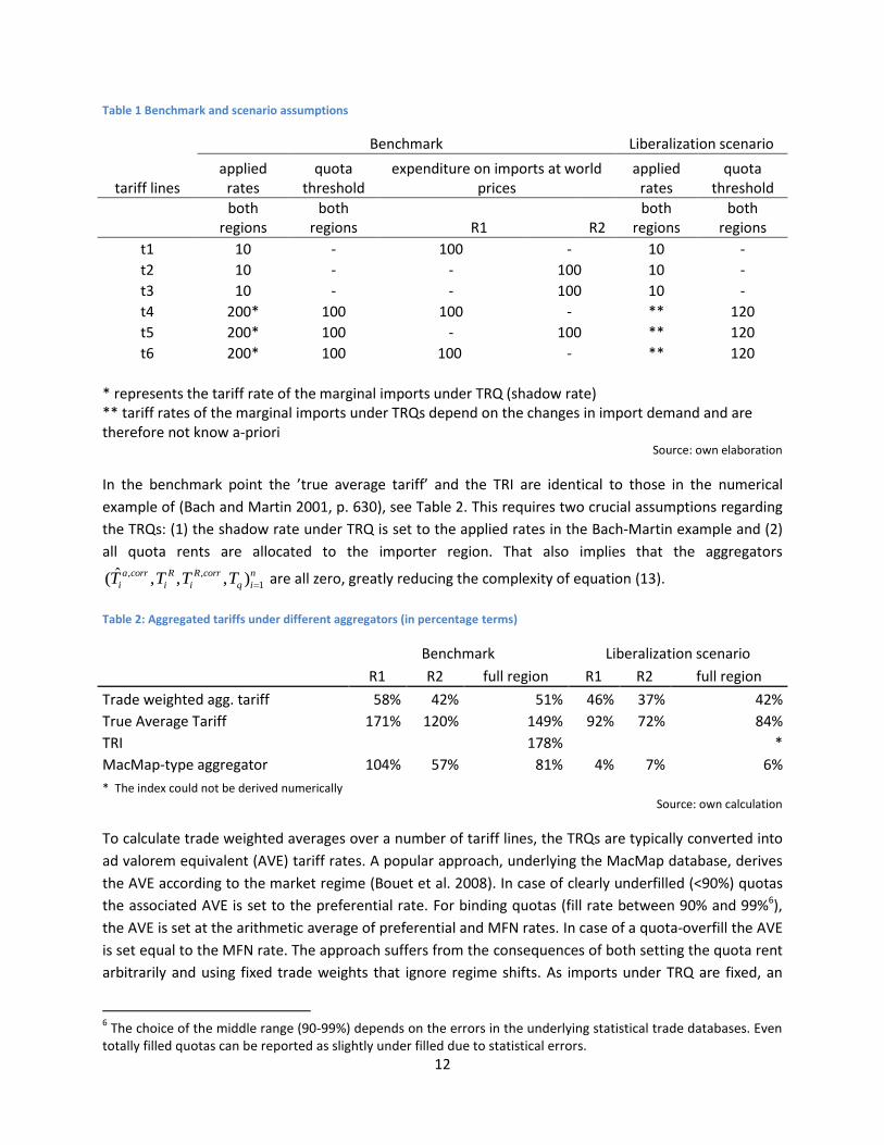
The benchmark data on imports and expenditures are set to be identical to those in Bach and Martin

(2001, p. 630) in order to make a direct comparison possible (Table 1). A dispersed tariff structure is

assumed over six tariff lines. Expenditure on the domestic goods equals to 2000 while the substitution

elasticity is set to 2. In order to illustrate the extended tariff aggregation technique, some tariff lines are

protected by TRQs with zero preferential rates and high MFN rates such that TRQs are filled.

Consequently, shadow rates, and so quota rents, are positive in the benchmark. The illustrative trade

liberalization scenario assumes no tariff reduction, as was in the case in Bach and Martin (2001), but an

expansion of the quota thresholds.

12

Table 1 Benchmark and scenario assumptions

Benchmark Liberalization scenario

tariff lines applied

rates quota

threshold expenditure on imports at world

prices applied

rates quota

threshold

both regions

both regions R1 R2

both regions

both regions

t1 10 - 100 - 10 -

t2 10 - - 100 10 -

t3 10 - - 100 10 -

t4 200* 100 100 - ** 120

t5 200* 100 - 100 ** 120

t6 200* 100 100 - ** 120

* represents the tariff rate of the marginal imports under TRQ (shadow rate) ** tariff rates of the marginal imports under TRQs depend on the changes in import demand and are therefore not know a-priori

Source: own elaboration

In the benchmark point the ’true average tariff’ and the TRI are identical to those in the numerical

example of (Bach and Martin 2001, p. 630), see Table 2. This requires two crucial assumptions regarding

the TRQs: (1) the shadow rate under TRQ is set to the applied rates in the Bach-Martin example and (2)

all quota rents are allocated to the importer region. That also implies that the aggregators ,

1

,ˆ( , , ),a corr R R corr

ii i i

n

qT T T T are all zero, greatly reducing the complexity of equation (13).

Table 2: Aggregated tariffs under different aggregators (in percentage terms)

Benchmark Liberalization scenario

R1 R2 full region R1 R2 full region

Trade weighted agg. tariff 58% 42% 51% 46% 37% 42%

True Average Tariff 171% 120% 149% 92% 72% 84%

TRI

178%

*

MacMap-type aggregator 104% 57% 81% 4% 7% 6%

* The index could not be derived numerically

Source: own calculation

To calculate trade weighted averages over a number of tariff lines, the TRQs are typically converted into

ad valorem equivalent (AVE) tariff rates. A popular approach, underlying the MacMap database, derives

the AVE according to the market regime (Bouet et al. 2008). In case of clearly underfilled (<90%) quotas

the associated AVE is set to the preferential rate. For binding quotas (fill rate between 90% and 99%6),

the AVE is set at the arithmetic average of preferential and MFN rates. In case of a quota-overfill the AVE

is set equal to the MFN rate. The approach suffers from the consequences of both setting the quota rent

arbitrarily and using fixed trade weights that ignore regime shifts. As imports under TRQ are fixed, an

6 The choice of the middle range (90-99%) depends on the errors in the underlying statistical trade databases. Even

totally filled quotas can be reported as slightly under filled due to statistical errors.

13

expansion of a binding quota typically delivers a huge drop in the AVE tariff rate (from the MFN rate to

the middle point of the preferential and the MFN rates) and in the resulting MacMap-type aggregator.

The same might also happen if TRQs are moderately overfilled. This is an extreme case of what has

already been reported in the literature, that fix weighted aggregators underestimate the level of trade

restriction and inconsistently measure the gains from trade liberalization (Kee et al. 2008).

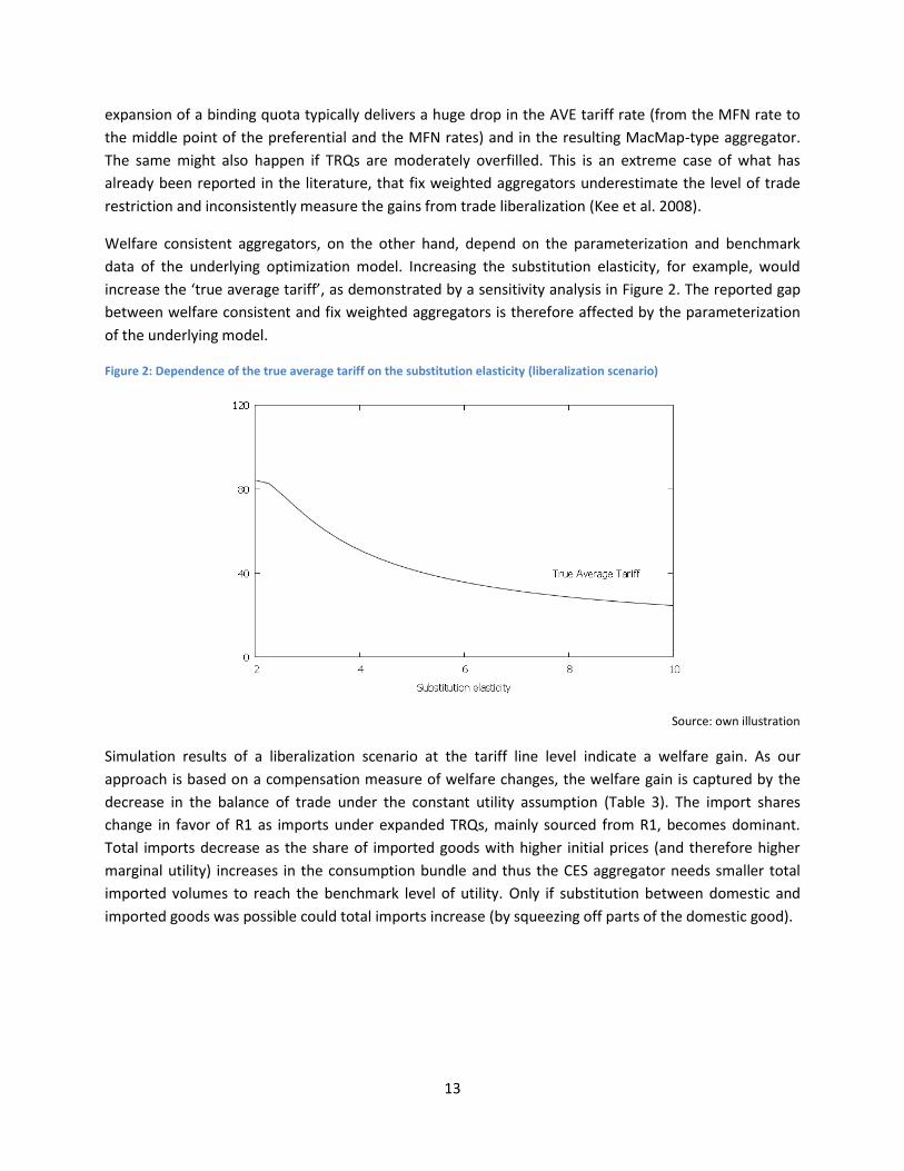
Welfare consistent aggregators, on the other hand, depend on the parameterization and benchmark

data of the underlying optimization model. Increasing the substitution elasticity, for example, would

increase the ‘true average tariff’, as demonstrated by a sensitivity analysis in Figure 2. The reported gap

between welfare consistent and fix weighted aggregators is therefore affected by the parameterization

of the underlying model.

Figure 2: Dependence of the true average tariff on the substitution elasticity (liberalization scenario)

Source: own illustration

Simulation results of a liberalization scenario at the tariff line level indicate a welfare gain. As our

approach is based on a compensation measure of welfare changes, the welfare gain is captured by the

decrease in the balance of trade under the constant utility assumption (Table 3). The import shares

change in favor of R1 as imports under expanded TRQs, mainly sourced from R1, becomes dominant.

Total imports decrease as the share of imported goods with higher initial prices (and therefore higher

marginal utility) increases in the consumption bundle and thus the CES aggregator needs smaller total

imported volumes to reach the benchmark level of utility. Only if substitution between domestic and

imported goods was possible could total imports increase (by squeezing off parts of the domestic good).

14

Table 3: Welfare results at the tariff line level (‘true’ values in value terms)

Benchmark Liberalization scenario

R1 R2 full region R1 R2 full region

Expenditure on imports at domestic p. 710 520 1230 546 363 910

Tariff revenues (incl. quota rent) at domestic p. 410 220 630 252 134 386

Expenditure on imports at world p. 300 300 600 295 229 524

Total expenditure at domestic p.

3230

2910

Balance of trade at domestic p.

600

524 Source: own calculation

The ‘true’ values calculated with the tariff line model are compared to test simulations with the different

tariff aggregators in Table 4. The optimal combination of the aggregators , ,ˆ ˆ( , ), , , ,a a corr R R corr

qT T T T T T

reproduces the change in overall welfare, total expenditure and tariff revenues (last two columns).

Furthermore, the regionally extended aggregators reproduce expenditure and tariff revenues not only in

total, but also with respect to imports from specific exporters. Clearly, the conventional MacMap-type

aggregators deliver biased welfare results, even if they are calculated at a finer geographical resolution7.

Table 4: Welfare results of the test runs with different tariff aggregators (percentage difference to ‘true’ values)

Welfare item Regional/total MacMap-type agg.

MacMap-type agg. (regional version)

Optimal combination

Optimal combination

(regional version)

Tariff revenues

R1 -93% -95% -4% 0%

R2 -92% -90% 7% 0%

full region -93% -94% 0% 0%

Expenditure on imports (at domestic prices)

R1 -40% -40% 4% 0%

R2 -47% -48% -7% 0%

full region -43% -43% 0% 0%

Total expenditure full region -13% -13% 0% 0%

Balance of trade full region -6% -6% 0% 0% Source: own calculation

Homothetic preferences imply that the composition of the optimal consumption bundle (the shares) is

independent of total consumer expenditure. As quota rents are modeled as lump-sum transfers to

consumers, quota allocation parameters have no impact on the optimal bundle either. On the other

hand, the TRI index is strongly affected by quota allocation parameters because quota rents directly

enter in the balance of trade condition of the TRI calculation. Allowing part of the quota rent being

allocated to exporter countries would quite intuitively increase the TRI as the TRI summarizes the impact

of trade restrictions on the own country’s welfare. If some of the quota rent escapes to the rest of the

world, the impact of the TRQ regime on the home country welfare must be stronger than before.

Similarly, low rent retaining rates result in lower quota rents retained in the home country and in higher

7 The regional version of the MacMap-type aggregator is calculated as trade weighted averages over imports from

specific exporter sub-regions.

15

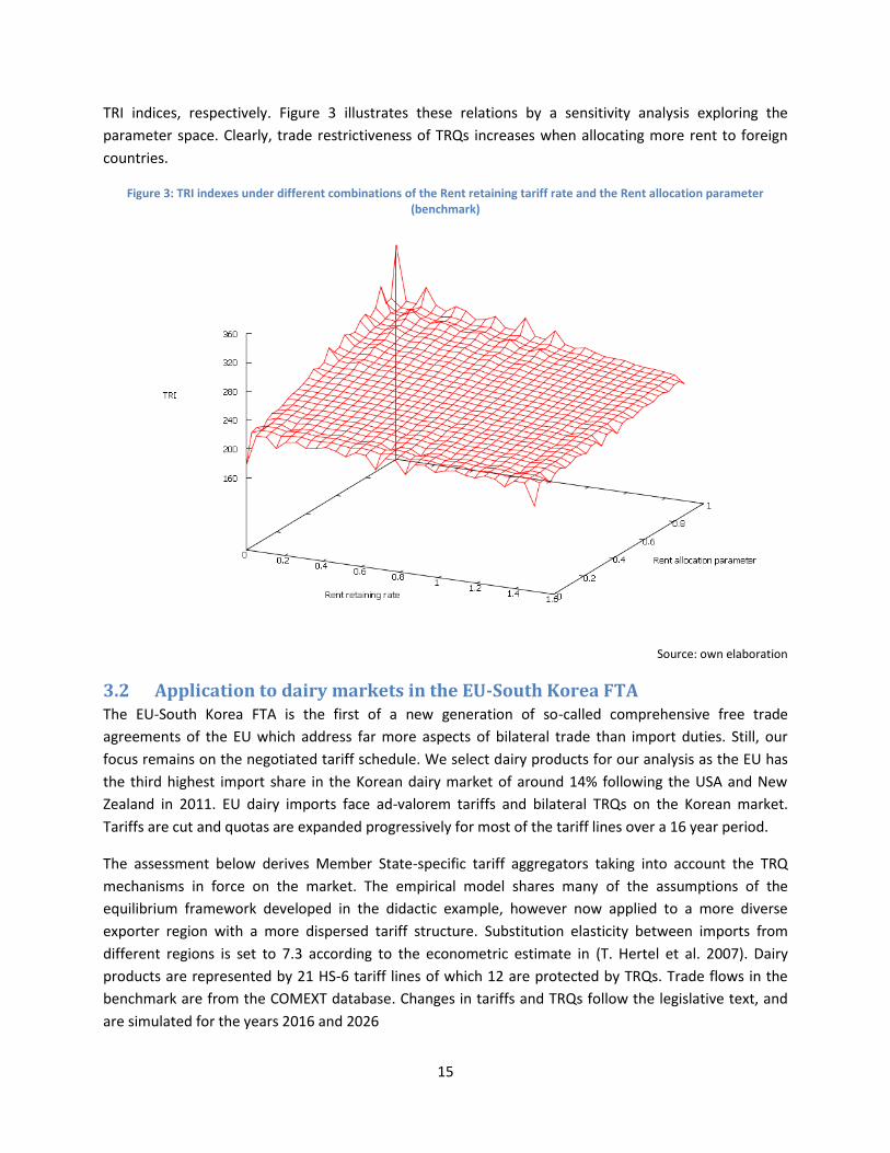
TRI indices, respectively. Figure 3 illustrates these relations by a sensitivity analysis exploring the

parameter space. Clearly, trade restrictiveness of TRQs increases when allocating more rent to foreign

countries.

Figure 3: TRI indexes under different combinations of the Rent retaining tariff rate and the Rent allocation parameter (benchmark)

Source: own elaboration

3.2 Application to dairy markets in the EU-South Korea FTA The EU-South Korea FTA is the first of a new generation of so-called comprehensive free trade

agreements of the EU which address far more aspects of bilateral trade than import duties. Still, our

focus remains on the negotiated tariff schedule. We select dairy products for our analysis as the EU has

the third highest import share in the Korean dairy market of around 14% following the USA and New

Zealand in 2011. EU dairy imports face ad-valorem tariffs and bilateral TRQs on the Korean market.

Tariffs are cut and quotas are expanded progressively for most of the tariff lines over a 16 year period.

The assessment below derives Member State-specific tariff aggregators taking into account the TRQ

mechanisms in force on the market. The empirical model shares many of the assumptions of the

equilibrium framework developed in the didactic example, however now applied to a more diverse

exporter region with a more dispersed tariff structure. Substitution elasticity between imports from

different regions is set to 7.3 according to the econometric estimate in (T. Hertel et al. 2007). Dairy

products are represented by 21 HS-6 tariff lines of which 12 are protected by TRQs. Trade flows in the

benchmark are from the COMEXT database. Changes in tariffs and TRQs follow the legislative text, and

are simulated for the years 2016 and 2026

16

Following the compensation variation approach of Bach and Martin, simulations are performed under

the fix utility assumption. Adjustments in the balance of trade, i.e. changes in the financial inflow

necessary to close the balance, are then indicating the monetary compensation needed to leave overall

welfare in the economy unchanged. Substitution between domestic and imported goods in the

consumption bundle is ruled out by the fix demand for the domestic good assumption.

The composition of Korean dairy imports from single EU countries is heterogeneous, leading to

differences in the calculated regional tariff aggregators (Table 5). Aggregated tariffs for those countries

exporting more under TRQs are typically lower, as they take advantage of the preferential market access.

The relative size of the derived tariff aggregators are in line with the findings of Manole and Martin

(2005): assuming the CES functional form and positive substitution elasticities, the tariff revenue

aggregator is always larger than or equal to the weighted average tariff and lower or equal than the ‘true

average tariff’. The comparison also reveals that trade weighted averages largely underestimates the

welfare-consistent ones.

Table 5: Tariff aggregators in percentage terms

True Average

Tariff

Tariff revenue

agg.

Trade weighted

agg. MacMap-type agg.

2010

Belgium 149%

47% 95%

Germany 163%

52% 114%

France 105%

22% 34%

Netherlands 119%

34% 62%

Rest of EU 91%

26% 43%

EU 134% 89% 40% 126%

2016

Belgium 131%

34% 68%

Germany 138%

28% 100%

France 73%

7% 15%

Netherlands 86%

15% 35%

Rest of EU 52%

5% 12%

EU 121% 58% 28% 120%

2026

Belgium 104%

14% 61%

Germany 127%

19% 98%

France 63%

2% 12%

Netherlands 65%

3% 22%

Rest of EU 45%

3% 7%

EU 110% 35% 18% 117% Source: own calculation

17

A remarkable outcome of our simulations is that the trade balance is worsening in the course of the FTA

implementation (Table 6). Decreasing welfare in the small country case as an impact of trade

liberalization seems to contradict basic results of trade economy. An important point to recognize is,

however, that by simulating under fix utility and without factor in impacts on tariff revenues in the

consumer decision problem8, the balance of trade condition becomes non-binding. More precisely, it is

the variable financial inflow that closes the trade balance in our framework, and not anymore the

equivalence of excess supply and import demand. The standard welfare calculation is also further

complicated by the assumption that producer prices are independent of trade policies and so changes in

producer surplus are ruled out. As a direct consequence, there is nothing left to guarantee a welfare

improvement in trade liberalization scenarios. In our simulation results cutting import tariffs implies a

relatively small decrease in consumer expenditures that does not offset the losses in tariff revenues and

therefore deteriorates the balance of trade.

Table 6: Welfare-related simulation results for South Korea

2010 2016 2026

Total consumer expenditure, at domestic p.

Total consumer expenditure, at domestic p. Mio.EUR 1003 961 928

Expenditure on imports, domestic p.

Expenditure on imports, domestic p. Mio.EUR 727 685 652

Expenditure on imports, world p.

Expenditure on imports, world p. Mio.EUR 439 496 533

Expenditure on domestic good, domestic p.

Expenditure on domestic good, domestic p. Mio.EUR 276 276 276

Tariff revenues, at domestic p.

Tariff revenues, at domestic p. Mio.EUR 277 179 109

Quota rents, at domestic p. Quota rents, at domestic p. Mio.EUR 11 10 10

Financial inflow* Balance of trade* Mio.EUR 439 496 533

TRI TRI % 195% * The balance of trade is defined as total consumer expenditures minus government revenues from

border protection instruments minus the value of the domestically produced good (fix in simulations) Source: own calculation

In order to evaluate the impact of choosing different tariff aggregators, we perform a simulation exercise

by plugging in the tariff aggregators in a model version featuring one single EU region only. The

simulated results are then systematically compared to those derived with the model operating at the

tariff line level (Table 7). The regional extension of Anderson’s optimal tariff combination clearly

outperform the standard one in exactly reproducing welfare results of the tariff line model at the finer

geographical resolution. Calculating conventional (MacMap-type) aggregators at the regional scale,

however, does not significantly improve the welfare-consistency of aggregate model results.

8 The underlying behavioral assumption is that each individual consumer is too small to change tariff revenues

significantly with the adjustments in his consumption bundle. Therefore individuals do not take into account the change they imply in tariff revenues in their consumption decisions (Gilbert and Tower 2012, page 159).

18

Table 7: Relative bias in reproducing the true welfare items with different tariff aggregators (year 2016)

2016

MacMap type (uniform across all exporters)

MacMap type (different across exporters)

Anderson's optimal combination

Anderson's optimal combination -- regional extension

Expenditure on domestic good, domestic p.

0% 0% 0% 0%

Expenditure on imports, domestic p. imports originated in

Belgium

35% 46% 35% 0%

Germany

62% -42% 63% 0%

France

-79% 145% -78% 0%

Netherlands -65% 49% -65% 0%

Rest of EU -90% 34% -90% 0%

Rest of the World 49% -87% 50% 0%

Total

0% -20% 0% 0%

Total consumer expenditure, at domestic p.

0% -14% 0% 0%

Gov. revenue from border protection imports originated in

Belgium

114% 72% 9% 0%

Germany

211% 3% 59% 0%

France

71% 380% -13% 0%

Netherlands 27% 159% -35% 0%

Rest of EU -2% 165% -50% 0%

Rest of the World 98% -81% 1% 0%

Total

96% -30% 0% 0%

Balance of trade

-37% -16% 0% 0% Source: own calculation

The test runs with the MacMap-type aggregators resulted in higher welfare gains than the ‘true’ impact

calculated with the tariff line model. Both the drop in total consumer expenditure to reach the same

utility and the improvement in the balance of trade were pronounced. This impact is largely due to the

AVE representation of TRQs. Even moderate quota expansions are perceived by the MacMap-type

aggregator as large reductions in the AVE, if the quota fill rate is close to 100% in the calibration point,

and the preferential rate is significantly lower than the MFN one. The MacMap-type aggregator

therefore overestimates welfare gains and the trade facilitating impact of quota expansions.

19

The standard result in the literature is that fixed weighted aggregators underestimate welfare gains.

Laborde et al. (2011) find that conventional tariff aggregators underestimate the gains in real income

from global trade liberalization by around 76% at the global scale. Anderson (2009), simulating a

unilateral trade liberalization for India, reports that e.g. efficiency gains are dramatically underestimated

with fixed weighted aggregators (¼ to 1/50 of the true gains). Our results indicate that the opposite

direction is also possible under more complex trade policy instruments such as TRQs.

4 Summary and conclusions Although its strong theoretical foundations have been already developed, welfare consistent tariff

aggregation has not yet gained ground in the impact assessment of FTAs. In this paper, we show that it is

numerically feasible to derive welfare consistent tariff aggregators from data at the detailed tariff line

level. In order to tackle the bilateral aspects of FTAs, we extend the Anderson (2009) framework of

welfare consistent aggregators with an explicit regional dimension. Specifically, we develop a sequential

numerical method to derive regional versions of the so-called ‘true average tariff’ under the assumption

of separable homotheticity. Flexible and welfare consistent tariff aggregation is then possible by

combining the regional aggregators in the balance-of-trade condition of our modeling framework.

The Anderson framework is not only flexible in terms of introducing the explicit regional dimension to

the tariff aggregation problem. It is also straightforward to include complex border protection measures,

such as TRQs. We define a combination of six tariff aggregators in a modified balance of trade condition

to aggregate tariffs and TRQs in a welfare consistent manner. The technique is capable of addressing

quota rent allocation directly. The importance of the (largely unknown) rent allocation on simulation

results is illustrated through a dedicated sensitivity analysis.

The extended tariff aggregation framework is applied both to a didactic example and to evaluation of the

Korean dairy market in the EU-South Korea FTA. Our results support the previous findings in the

literature, that conventional fixed weighted tariff aggregators introduce a serious bias in aggregated

welfare results.

The tariff aggregation clearly depends on the parameterization and input data of the underlying model,

and so encapsulates much more information than the tariff structure itself, as demonstrated with a

sensitivity analysis based on different substitution elasticities. The approach is constrained by the usual

limitations of Armington models, e.g. it is unable to factor in the effect of (prohibitive) tariffs leading to

zero-trade flows9. Furthermore, our approach is based on a compensation measure of welfare impacts,

while standard applied equilibrium modeling practices typically apply money metric measures. A direct

implementation in AEMs thus first requires setting up simulations under the fix utility assumption. Last

but not least, unlike conventional aggregators, the welfare consistent aggregators require additionally

data on consumption at the aggregate level.

9 The MacMap methodology, for example, builds on average trade shares from similar countries to overcome the

zero trade issue. Such an approach could potentially be used with welfare consistent aggregators as well.

20

These findings directly lead to recommendations for empirical work. Against the background and findings

that welfare consistent aggregators outperform simple trade weighted averages in replicating welfare

impacts, their use for pre-model aggregation can be clearly recommended. This is especially true for

modeling exercises aiming at quantifying the impacts of FTAs. The GAMS code available from the authors

underlines that its application is nowadays no longer a demanding exercise once data at the tariff line

are available. It remains for further research to test the extended aggregation technique in large-scale

AEMs, covering a large number of interacting markets.

5 References Anderson, James E, and J. Peter Neary. 2005. Measuring the Restrictiveness of International Trade Policy.

Cambridge, Mass.: MIT Press. Anderson, James E. 2009. “Consistent Trade Policy Aggregation*.” International Economic Review 50 (3):

903–27. doi:10.1111/j.1468-2354.2009.00553.x. Anderson, James E., and J. Peter Neary. 1994. “Measuring the Restrictiveness of Trade Policy.” The World

Bank Economic Review 8 (2): 151–69. doi:10.1093/wber/8.2.151. Bach, Christian F, and Will Martin. 2001. “Would the Right Tariff Aggregator for Policy Analysis Please

Stand Up?” Journal of Policy Modeling 23 (6): 621–35. doi:10.1016/S0161-8938(01)00077-1. Bouet, Antoine, Yvan Decreux, Lionel Fontagne, Sebastien Jean, and David Laborde. 2008. “Assessing

Applied Protection across the World.” Review of International Economics 16 (5): 850–63. Boughner, Devry S., Harry de Gorter, and Ian M. Sheldon. 2000. “The Economics of Two-Tier Tariff-Rate

Import Quotas in Agriculture.” Agricultural and Resource Economics Review 29 (1): 58–69. Bureau, Jean-Christophe, and Luca Salvatici. 2004. “WTO Negotiations on Market Access in Agriculture: A

Comparison of Alternative Tariff Cut Proposals for the EU and the US.” Topics in Economic Analysis & Policy 4 (1).

Deaton, Augus, and John Muellbauer. 1980. Economics and Consumer Behavior. Cambridge: Cambridge University Press.

Gilbert, John P, and Edward Tower. 2012. Introduction to Numerical Simulation for Trade Theory and Policy. Singapore: World Scientific.

Grant, Jason H., Thomas W. Hertel, and Thomas F. Rutherford. 2007. “Tariff Line Analysis of U.S. and International Dairy Protection.” Agricultural Economics 37: 271–80. doi:10.1111/j.1574-0862.2007.00251.x.

Guimbard, Houssein, Sébastien Jean, Mondher Mimouni, and Xavier Pichot. 2012. MAcMap-HS6 2007, an Exhaustive and Consistent Measure of Applied Protection in 2007. Working Paper 2012-10. CEPII research center.

Hertel, Thomas, David Hummels, Maros Ivanic, and Roman Keeney. 2007. “How Confident Can We Be of CGE-Based Assessments of Free Trade Agreements?” Economic Modelling 24 (4): 611–35. doi:10.1016/j.econmod.2006.12.002.

Hertel, Thomas W. 1999. Global Trade Analysis: Modeling and Applications. Cambridge; New York: Cambridge University Press.

Horridge, Mark. 2008. “GTAPAgg: Data Aggregation Program (Chapter 5).” In Global Trade, Assistance, and Production: The GTAP 7 Data Base.

Horridge, Mark, and David Laborde. 2008. “TASTE a Program to Adapt Detailed Trade and Tariff Data to GTAP-Related Purposes.” In 11th Annual Conference on Global Economic Analysis, Helsinki, Finland.

21

Junker, Franziska, and Thomas Heckelei. 2012. “TRQ-Complications: Who Gets the Benefits When the EU Liberalizes Mercosur’s Access to the Beef Markets?” Agricultural Economics 43 (2): 215–31. doi:10.1111/j.1574-0862.2011.00578.x.

Kee, Hiau Looi, Alessandro Nicita, and Marcelo Olarreaga. 2008. “Import Demand Elasticities and Trade Distortions.” Review of Economics and Statistics 90 (4): 666–82. doi:10.1162/rest.90.4.666.

Laborde, David, Will Martin, and Dominiquie van der Mensbrugghe. 2011. Measuring the Impacts of Global Trade Reform with Optimal Aggregators of Distortions. 01123. Discussion Papers. IFPRI: Markets, Trade and Institutions Division.

Manole, V., and W. Martin. 2005. “Keeping the Devil in the Details: A Feasible Approach to Aggregating Trade Distortions.” In Dublin.

Martin, William J. 1997. “Measuring Welfare Changes with Distortions.” In Applied Methods for Trade Policy Analysis. Cambridge University Press.

Narayanan, Badri G., Thomas W. Hertel, and J. Mark Horridge. 2010. “Disaggregated Data and Trade Policy Analysis: The Value of Linking Partial and General Equilibrium Models.” Economic Modelling 27 (3): 755–66. doi:10.1016/j.econmod.2010.01.018.

Pelikan, Janine, and Martina Brockmeier. 2008. “Methods to Aggregate Import Tariffs and Their Impacts on Modeling Results.” Journal of Economic Integration 23 (3): 685–708.

Rutherford, Thomas F. 1995. “Extension of GAMS for Complementarity Problems Arising in Applied Economic Analysis.” Journal of Economic Dynamics and Control 19 (8): 1299–1324. doi:10.1016/0165-1889(94)00831-2.

World Trade Organization. 2012. Tariff Quota Administration Methods and Fill Rates 2002-2011.

Appendix A

In order to show the equivalence of 1( )i

n

i and 1( )i

n

i we first reformulate the definition of the latter in

equation (9), by applying Euler’s theorem on homogeneous functions:

) ( · ·( {1 }

· {

, ( ), ) ,

1 },

ic c c ic c i i

i j ii i

c c ii

i i

i j

j

i

p p pp p ip p p n

p p p

p pi n

p p

p p p

p p

By substituting the above expression back into equation (8), we show that the conditions for the 1( )i

n

i

aggregators are satisfied too:

1( ), , ( ), ) · (( , ).c i cc n i i c

i ii i

p pp p p p p p

p pp

Appendix B Anderson’s optimal combination of tariff aggregators in the balance of trade function can be substituted

with an equivalent combination of exporter-specific aggregators, in case of separable homothetic

consumer preferences.

22

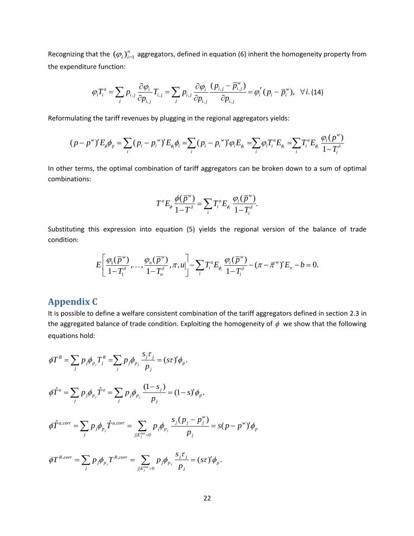
Recognizing that the 1( )i

n

i aggregators, defined in equation (6) inherit the homogeneity property from

the expenditure function:

,,

, , ,

, , ,

( )( ), .

i ji ii i j i j i j i i

i j i

w

i

j i j

ja w

i i

j j

ip

p pT p T p

pp

pp

(14)

Reformulating the tariff revenues by plugging in the regional aggregators yields:

(

( ) ( ) ( )1

)i i i i

ww w w i

p

a a

i i

i i

i i i i i i

i

i

i i

pp p E p p E p p E T E T E

T

In other terms, the optimal combination of tariff aggregators can be broken down to a sum of optimal

combinations:

.1 1

( )( )i

wa

i

i i

wa iT E T E

T T

pp

Substituting this expression into equation (5) yields the regional version of the balance of trade

condition:

1

1

( ) (, , ( ) 0.

1

)( ), ,

1 1i

w wwwian

i

in i

E T E E bT T

ppu

T

p

Appendix C It is possible to define a welfare consistent combination of the tariff aggregators defined in section 2.3 in

the aggregated balance of trade condition. Exploiting the homogeneity of we show that the following

equations hold:

)( .j j

R

p p

j jR

j j j

j j j

p

sT p T p s

p

(1(1 )

)ˆ .ˆ

j j

j

j j

j j j

a a

p p p

sp pT s

pT

| 0

, ,( )

)ˆ (ˆj j

outj

w

ja corr a corr w

p

j j

j j

j j E j

p p

s p pp p s p p

pT T

| 0

, , ( ) .j j

outj

R corr R corr

p p

j j

j j

j

p

j E j

Ts

p p sp

T

23

Substituting these expressions in the tariff revenue part of equation (10) yields:

, ,

) ( ) ( )

( ) (

(1 )(

) (1 )( ( )) ( ( )

ˆ

)

(

ˆ ( )

)

1

w q w out

p p

q w q w out out w out

p p p p

R a a corr R corr w out

w

s s p p I s p p s E q I

s I I s p p E I s I s p p s qI

E T E T E E s

E

E s

p

p p E

p s qI

E Tp

T

E

T T

,ˆ ˆ .1

( )wR a a corr R

qT E T TT

pT

Substituting this back to the balance of trade condition results in equation (12).