week 13: margins and interpreting results - denver, … 13: margins and interpreting results ......
TRANSCRIPT

Week 13: Margins and interpreting results
Marcelo Coca Perraillon
University of ColoradoAnschutz Medical Campus
Health Services Research Methods IHSMP 7607
2017
c©2017 PERRAILLON ARR 1

Outline
Why do we need them?
A collection of terms
1 Average Marginal Effects (AME)2 Maginal Effect at the Mean (MEM)3 Marginal Effects at Representative values (MER)
Interactions
Examples
c©2017 PERRAILLON ARR 2
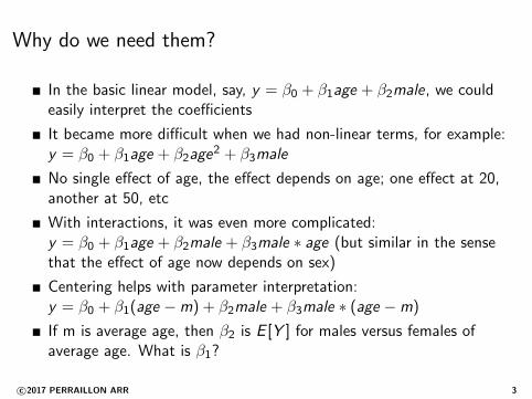
Why do we need them?
In the basic linear model, say, y = β0 + β1age + β2male, we couldeasily interpret the coefficients
It became more difficult when we had non-linear terms, for example:y = β0 + β1age + β2age
2 + β3male
No single effect of age, the effect depends on age; one effect at 20,another at 50, etc
With interactions, it was even more complicated:y = β0 + β1age + β2male + β3male ∗ age (but similar in the sensethat the effect of age now depends on sex)
Centering helps with parameter interpretation:y = β0 + β1(age −m) + β2male + β3male ∗ (age −m)
If m is average age, then β2 is E [Y ] for males versus females ofaverage age. What is β1?
c©2017 PERRAILLON ARR 3
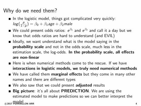
Why do we need them?
In the logistic model, things got complicated very quickly:log( p
1−p ) = β0 + β1age + β2male
We could present odds ratios: eβ1 and eβ2 and call it a day but weknow that odds ratios are hard to understand (and EVIL)
Ideally, we want understand what is the model saying in theprobability scale and not in the odds scale, much less in theestimation scale, the log-odds. In the probability scale, all effectsare non-linear
Here is when numerical methods come to the rescue. If we haveinteractions in logistic models, we truly need numerical methods
We have called them marginal effects but they come in many othernames and there are different types
We also saw that we could present adjusted results
Big picture: it’s all about PREDICTION. We are using theestimated model to make predictions so we can better interpret themodel
c©2017 PERRAILLON ARR 4
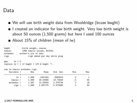
Data
We will use birth weight data from Wooldridge (bcuse bwght)
I created an indicator for low birth weight. Very low birth weight isabout 50 ounces (1,500 grams) but here I used 100 ounces
About 15% of children (mean of lw)
bwght birth weight, ounces
faminc 1988 family income, $1000s
motheduc mother’s yrs of educ
cigs cigs smked per day while preg
gen lw = 0
replace lw = 1 if bwght < 100 & bwght ~= .
sum lw faminc motheduc cigs
Variable | Obs Mean Std. Dev. Min Max
-------------+---------------------------------------------------------
lw | 1,388 .1491354 .3563503 0 1
faminc | 1,388 29.02666 18.73928 .5 65
motheduc | 1,387 12.93583 2.376728 2 18
cigs | 1,388 2.087176 5.972688 0 50
c©2017 PERRAILLON ARR 5
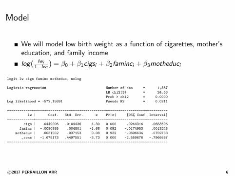
Model
We will model low birth weight as a function of cigarettes, mother’seducation, and family income
log( lwi1−lwi
) = β0 + β1cigsi + β2faminci + β3motheduci
logit lw cigs faminc motheduc, nolog
Logistic regression Number of obs = 1,387
LR chi2(3) = 24.63
Prob > chi2 = 0.0000
Log likelihood = -572.15891 Pseudo R2 = 0.0211
------------------------------------------------------------------------------
lw | Coef. Std. Err. z P>|z| [95% Conf. Interval]
-------------+----------------------------------------------------------------
cigs | .0449006 .0104436 4.30 0.000 .0244316 .0653696
faminc | -.0080855 .004801 -1.68 0.092 -.0174953 .0013243
motheduc | .0031552 .037153 0.08 0.932 -.0696634 .0759738
_cons | -1.678173 .4497551 -3.73 0.000 -2.559676 -.7966687
------------------------------------------------------------------------------
c©2017 PERRAILLON ARR 6
Model
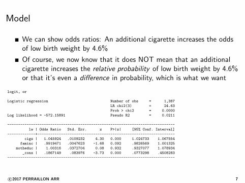
We can show odds ratios: An additional cigarette increases the oddsof low birth weight by 4.6%
Of course, we now know that it does NOT mean that an additionalcigarette increases the relative probability of low birth weight by 4.6%or that it’s even a difference in probability, which is what we want
logit, or
Logistic regression Number of obs = 1,387
LR chi2(3) = 24.63
Prob > chi2 = 0.0000
Log likelihood = -572.15891 Pseudo R2 = 0.0211
------------------------------------------------------------------------------
lw | Odds Ratio Std. Err. z P>|z| [95% Conf. Interval]
-------------+----------------------------------------------------------------
cigs | 1.045924 .0109232 4.30 0.000 1.024733 1.067554
faminc | .9919471 .0047623 -1.68 0.092 .9826569 1.001325
motheduc | 1.00316 .0372704 0.08 0.932 .9327077 1.078934
_cons | .1867149 .083976 -3.73 0.000 .0773298 .4508283
------------------------------------------------------------------------------
c©2017 PERRAILLON ARR 7
Model
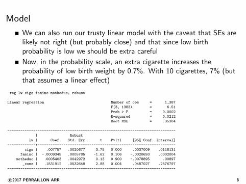
We can also run our trusty linear model with the caveat that SEs arelikely not right (but probably close) and that since low birthprobability is low we should be extra careful
Now, in the probability scale, an extra cigarette increases theprobability of low birth weight by 0.7%. With 10 cigarettes, 7% (butthat assumes a linear effect)
reg lw cigs faminc motheduc, robust
Linear regression Number of obs = 1,387
F(3, 1383) = 6.51
Prob > F = 0.0002
R-squared = 0.0212
Root MSE = .35304
------------------------------------------------------------------------------
| Robust
lw | Coef. Std. Err. t P>|t| [95% Conf. Interval]
-------------+----------------------------------------------------------------
cigs | .007757 .0020677 3.75 0.000 .0037009 .0118131
faminc | -.0009345 .0005785 -1.62 0.106 -.0020693 .0002004
motheduc | .0005403 .0042972 0.13 0.900 -.0078895 .00897
_cons | .1531912 .0532648 2.88 0.004 .0487027 .2576797
------------------------------------------------------------------------------
c©2017 PERRAILLON ARR 8
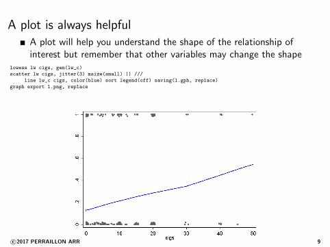
A plot is always helpfulA plot will help you understand the shape of the relationship ofinterest but remember that other variables may change the shape
lowess lw cigs, gen(lw_c)
scatter lw cigs, jitter(3) msize(small) || ///
line lw_c cigs, color(blue) sort legend(off) saving(l.gph, replace)
graph export l.png, replace
c©2017 PERRAILLON ARR 9
Before you get lost
We will see different ways of presenting results using the right model:a logistic model
We will do it using the scale of interest: the probability scale
We could have made life easier and explore the relationship using thelinear model
We know it is not quite right but we also know that it is easier tointerpret and probably not quite wrong
Not a bad a idea to start with a linear model and then switch tologistic (or probit)
c©2017 PERRAILLON ARR 10
Adjusting, review
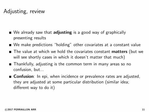
We already saw that adjusting is a good way of graphicallypresenting results
We make predictions “holding” other covariates at a constant value
The value at which we hold the covariates constant matters (but wewill see shortly cases in which it doesn’t matter that much)
Thankfully, adjusting is the common term in many areas so noconfusion, but...
Confusion: In epi, when incidence or prevalence rates are adjusted,they are adjusted at some particular distribution (similar idea;different way to do it)
c©2017 PERRAILLON ARR 11

Example
Say, we have trends in hip fractures that are increasing. It could bethat hip fractures are going up just because the population is gettingolder
So we want to “adjust” for the aging population and present adjustedtrends; in many cases, we don’t have individual level data so we can’trun a regression model
So calculate hip fractures by age group and year. Then hold agedistribution at one particular year and weight the rates using thoseweights
c©2017 PERRAILLON ARR 12
Excel example
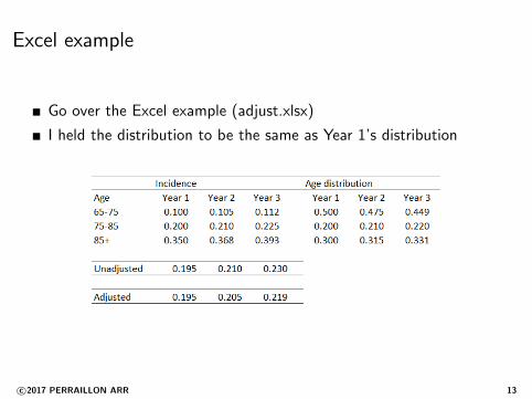
Go over the Excel example (adjust.xlsx)
I held the distribution to be the same as Year 1’s distribution
c©2017 PERRAILLON ARR 13
Adjusting, review
We learned how to adjust in multiple regression in the context of thelinear model
For example: what is the probability of low birth weight as a functionof cigarettes holding the other covariates constant?
We can hold the values constant at different values and compareadjusted trends or just keep them constant at their mean
No hard rules; depends on what we want to show or understand
c©2017 PERRAILLON ARR 14
Model adjusted
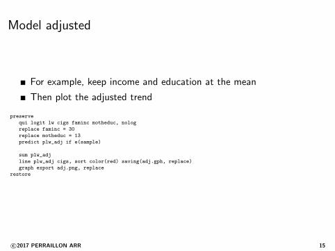
For example, keep income and education at the mean
Then plot the adjusted trend
preserve
qui logit lw cigs faminc motheduc, nolog
replace faminc = 30
replace motheduc = 13
predict plw_adj if e(sample)
sum plw_adj
line plw_adj cigs, sort color(red) saving(adj.gph, replace)
graph export adj.png, replace
restore
c©2017 PERRAILLON ARR 15
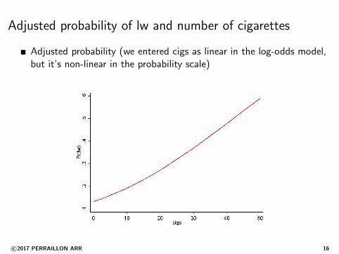
Adjusted probability of lw and number of cigarettes
Adjusted probability (we entered cigs as linear in the log-odds model,but it’s non-linear in the probability scale)
c©2017 PERRAILLON ARR 16
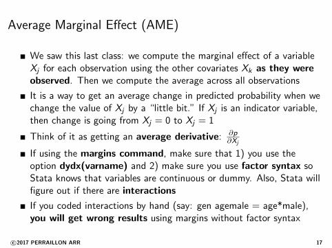
Average Marginal Effect (AME)
We saw this last class: we compute the marginal effect of a variableXj for each observation using the other covariates Xk as they wereobserved. Then we compute the average across all observations
It is a way to get an average change in predicted probability when wechange the value of Xj by a “little bit.” If Xj is an indicator variable,then change is going from Xj = 0 to Xj = 1
Think of it as getting an average derivative: ∂p∂Xj
If using the margins command, make sure that 1) you use theoption dydx(varname) and 2) make sure you use factor syntax soStata knows that variables are continuous or dummy. Also, Stata willfigure out if there are interactions
If you coded interactions by hand (say: gen agemale = age*male),you will get wrong results using margins without factor syntax
c©2017 PERRAILLON ARR 17
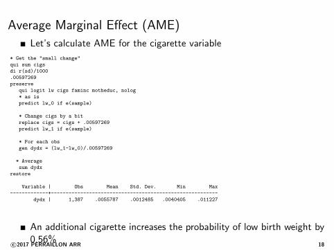
Average Marginal Effect (AME)
Let’s calculate AME for the cigarette variable
* Get the "small change"
qui sum cigs
di r(sd)/1000
.00597269
preserve
qui logit lw cigs faminc motheduc, nolog
* as is
predict lw_0 if e(sample)
* Change cigs by a bit
replace cigs = cigs + .00597269
predict lw_1 if e(sample)
* For each obs
gen dydx = (lw_1-lw_0)/.00597269
* Average
sum dydx
restore
Variable | Obs Mean Std. Dev. Min Max
-------------+---------------------------------------------------------
dydx | 1,387 .0055787 .0012485 .0040405 .011227
An additional cigarette increases the probability of low birth weight by0.56%
c©2017 PERRAILLON ARR 18

Average Marginal Effect (AME)
Replicate using margins command
. margins, dydx(cigs)
Average marginal effects Number of obs = 1,387
Model VCE : OIM
Expression : Pr(lw), predict()
dy/dx w.r.t. : cigs
------------------------------------------------------------------------------
| Delta-method
| dy/dx Std. Err. z P>|z| [95% Conf. Interval]
-------------+----------------------------------------------------------------
cigs | .0055782 .0012814 4.35 0.000 .0030666 .0080898
------------------------------------------------------------------------------
Same result
c©2017 PERRAILLON ARR 19
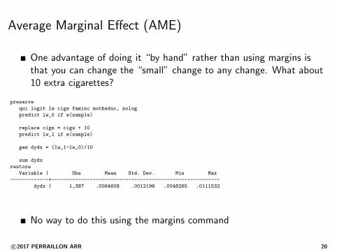
Average Marginal Effect (AME)
One advantage of doing it “by hand” rather than using margins isthat you can change the “small” change to any change. What about10 extra cigarettes?
preserve
qui logit lw cigs faminc motheduc, nolog
predict lw_0 if e(sample)
replace cigs = cigs + 10
predict lw_1 if e(sample)
gen dydx = (lw_1-lw_0)/10
sum dydx
restore
Variable | Obs Mean Std. Dev. Min Max
-------------+---------------------------------------------------------
dydx | 1,387 .0064608 .0012196 .0048265 .0111532
No way to do this using the margins command
c©2017 PERRAILLON ARR 20
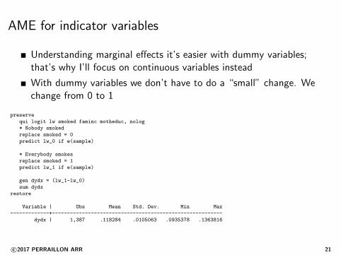
AME for indicator variables
Understanding marginal effects it’s easier with dummy variables;that’s why I’ll focus on continuous variables instead
With dummy variables we don’t have to do a “small” change. Wechange from 0 to 1
preserve
qui logit lw smoked faminc motheduc, nolog
* Nobody smoked
replace smoked = 0
predict lw_0 if e(sample)
* Everybody smokes
replace smoked = 1
predict lw_1 if e(sample)
gen dydx = (lw_1-lw_0)
sum dydx
restore
Variable | Obs Mean Std. Dev. Min Max
-------------+---------------------------------------------------------
dydx | 1,387 .118284 .0105063 .0935378 .1363816
c©2017 PERRAILLON ARR 21

AME for indicator variables
We can of course also use the margins command
qui logit lw smoked faminc motheduc, nolog
margins, dydx(smoked)
------------------------------------------------------------------------------
| Delta-method
| dy/dx Std. Err. z P>|z| [95% Conf. Interval]
-------------+----------------------------------------------------------------
smoked | .0988076 .0230959 4.28 0.000 .0535405 .1440748
------------------------------------------------------------------------------
qui logit lw i.smoked faminc motheduc, nolog
margins, dydx(smoked)
------------------------------------------------------------------------------
| Delta-method
| dy/dx Std. Err. z P>|z| [95% Conf. Interval]
-------------+----------------------------------------------------------------
1.smoked | .118284 .0322576 3.67 0.000 .0550602 .1815078
------------------------------------------------------------------------------
Note: dy/dx for factor levels is the discrete change from the base level.
Even though same margins statement, different results. The first oneis not what we wanted. The model did not use the factor syntax soStata didn’t go from 0 to 1; instead it used a “small” change
Smoking increases the probability of low birth weight by almost 12%points (yikes)
c©2017 PERRAILLON ARR 22
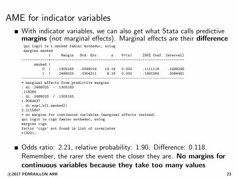
AME for indicator variables
With indicator variables, we can also get what Stata calls predictivemargins (not marginal effects). Marginal effects are their differencequi logit lw i.smoked faminc motheduc, nolog
margins smoked
| Margin Std. Err. z P>|z| [95% Conf. Interval]
-------------+----------------------------------------------------------------
smoked |
0 | .1305183 .0099014 13.18 0.000 .1111118 .1499248
1 | .2488023 .0304311 8.18 0.000 .1891584 .3084461
------------------------------------------------------------------------------
* marginal effects from predictive margins
. di .2488023 - .1305183
.118284
. di .2488023 / .1305183
1.9062637
. di exp(_b[1.smoked])
2.2115807
* no margins for continuous variables (marginal effects instead)
qui logit lw cigs faminc motheduc, nolog
margins cigs
factor ’cigs’ not found in list of covariates
r(322);
Odds ratio: 2.21, relative probability: 1.90. Difference: 0.118.Remember, the rarer the event the closer they are. No margins forcontinuous variables because they take too many values
c©2017 PERRAILLON ARR 23

Marginal Effect at the Mean (MEM)
We have left the values of the covariates as they were observedrather than holding them fixed at a certain value
We can also calculate marginal effects at the mean, much like whatwe did when we adjusted predictions
There is some discussion about which way is better (see Williams,2012): For example, does it make sense to hold male at 0.6 male?
Don’t waste too much time thinking about this. When wecalculate marginal effects, it doesn’t really matter at which value wehold the other covariates constant because we are taking differencesin effects
The difference will be so small that it is better to spend mentalresources somewhere else
c©2017 PERRAILLON ARR 24

Marginal Effect at the Mean (MEM)
Keep covariates at mean values instead
preserve
qui logit lw cigs faminc motheduc, nolog
* At mean
replace faminc = 29.02666
replace motheduc = 12.93583
predict lw_0 if e(sample)
*small change
replace cigs = cigs + .00597269
predict lw_1 if e(sample)
gen dydx = (lw_1-lw_0)/.00597269
sum dydx
restore
Variable | Obs Mean Std. Dev. Min Max
-------------+---------------------------------------------------------
dydx | 1,387 .0055649 .0010425 .0051894 .011212
MEM not that difference from AME
c©2017 PERRAILLON ARR 25
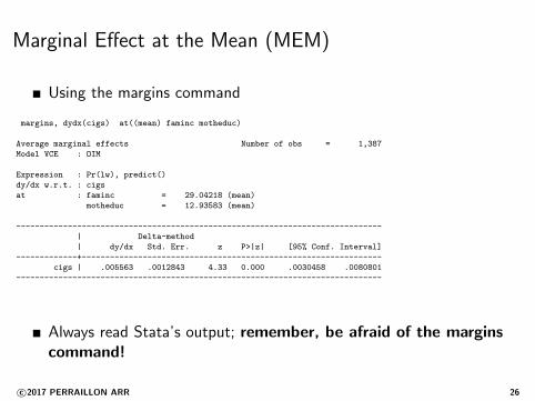
Marginal Effect at the Mean (MEM)
Using the margins command
margins, dydx(cigs) at((mean) faminc motheduc)
Average marginal effects Number of obs = 1,387
Model VCE : OIM
Expression : Pr(lw), predict()
dy/dx w.r.t. : cigs
at : faminc = 29.04218 (mean)
motheduc = 12.93583 (mean)
------------------------------------------------------------------------------
| Delta-method
| dy/dx Std. Err. z P>|z| [95% Conf. Interval]
-------------+----------------------------------------------------------------
cigs | .005563 .0012843 4.33 0.000 .0030458 .0080801
------------------------------------------------------------------------------
Always read Stata’s output; remember, be afraid of the marginscommand!
c©2017 PERRAILLON ARR 26

Marginal Effect at the Mean (MEM)
Not the same as using the atmeans option
margins, dydx(cigs) atmeans
Conditional marginal effects Number of obs = 1,387
Model VCE : OIM
Expression : Pr(lw), predict()
dy/dx w.r.t. : cigs
at : cigs = 2.088681 (mean)
faminc = 29.04218 (mean)
motheduc = 12.93583 (mean)
------------------------------------------------------------------------------
| Delta-method
| dy/dx Std. Err. z P>|z| [95% Conf. Interval]
-------------+----------------------------------------------------------------
cigs | .0055506 .0012879 4.31 0.000 .0030264 .0080749
------------------------------------------------------------------------------
One more time: please be careful with the margins command
c©2017 PERRAILLON ARR 27
Marginal effects at representative values (MER)
We can hold values at observed values (AME) or at mean values(MEM)
We could also choose representative values; values that are ofinterest. We did something similar when adjusting
For example, what is the marginal effect of an additional cigarette onthe probability of low birth weight at different levels of income, say10K, 20K, 30K and 40K?
We will do two by hand and the rest with the margins command
Leave other covariates as observed
c©2017 PERRAILLON ARR 28

Marginal effects at representative values (MER)
We will do it “by hand” for low income (10K) and higher income(40K)
preserve
qui logit lw cigs faminc motheduc, nolog
* income 10k
replace faminc = 10
predict lw_0_10 if e(sample)
replace cigs = cigs + .00597269
predict lw_1_10 if e(sample)
gen dydx10 = (lw_1_10-lw_0_10)/.00597269
* income 40k
replace faminc = 40
predict lw_0_40 if e(sample)
replace cigs = cigs + .00597269
predict lw_1_40 if e(sample)
gen dydx40 = (lw_1_40-lw_0_40)/.00597269
sum dydx*
restore
sum dydx*
Variable | Obs Mean Std. Dev. Min Max
-------------+---------------------------------------------------------
dydx10 | 1,387 .0061675 .0010195 .0056509 .011217
dydx40 | 1,387 .0052307 .001039 .0047328 .011197
c©2017 PERRAILLON ARR 29
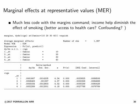
Marginal effects at representative values (MER)
Much less code with the margins command; income help diminish theeffect of smoking (better access to health care? Confounding? )
margins, dydx(cigs) at(faminc=(10 20 30 40)) vsquish
Average marginal effects Number of obs = 1,387
Model VCE : OIM
Expression : Pr(lw), predict()
dy/dx w.r.t. : cigs
1._at : faminc = 10
2._at : faminc = 20
3._at : faminc = 30
4._at : faminc = 40
------------------------------------------------------------------------------
| Delta-method
| dy/dx Std. Err. z P>|z| [95% Conf. Interval]
-------------+----------------------------------------------------------------
cigs |
_at |
1 | .0061667 .0014205 4.34 0.000 .0033825 .0089508
2 | .0058463 .001337 4.37 0.000 .0032258 .0084668
3 | .0055334 .0012803 4.32 0.000 .0030239 .0080428
4 | .0052289 .0012501 4.18 0.000 .0027788 .0076789
------------------------------------------------------------------------------
c©2017 PERRAILLON ARR 30
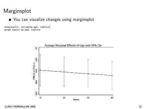
Marginsplot
You can visualize changes using marginsplot
marginsplot, saving(mp.gph, replace)
graph export mp.png, replace
c©2017 PERRAILLON ARR 31
Interactions
We have estimated the modellog( lwi
1−lwi) = β0 + β1cigsi + β2faminci + β3motheduci
We didn’t use interactions between cigarettes and income so we haveassumed the same effect regardless of income
In other words, same slope and and some intercept
We could add interactions and that’s when the margins command is alife saver because effects are hard to compute otherwise
c©2017 PERRAILLON ARR 32
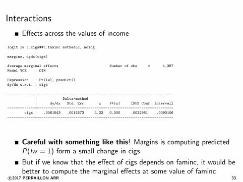
Interactions
Effects across the values of income
logit lw c.cigs##c.faminc motheduc, nolog
margins, dydx(cigs)
Average marginal effects Number of obs = 1,387
Model VCE : OIM
Expression : Pr(lw), predict()
dy/dx w.r.t. : cigs
------------------------------------------------------------------------------
| Delta-method
| dy/dx Std. Err. z P>|z| [95% Conf. Interval]
-------------+----------------------------------------------------------------
cigs | .0061543 .0014573 4.22 0.000 .0032981 .0090106
------------------------------------------------------------------------------
Careful with something like this! Margins is computing predictedP(lw = 1) form a small change in cigs
But if we know that the effect of cigs depends on faminc, it would bebetter to compute the marginal effects at some value of faminc
c©2017 PERRAILLON ARR 33
Interactions
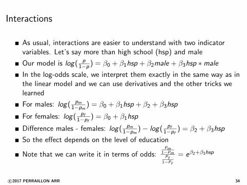
As usual, interactions are easier to understand with two indicatorvariables. Let’s say more than high school (hsp) and male
Our model is log( p1−p ) = β0 + β1hsp + β2male + β3hsp ∗male
In the log-odds scale, we interpret them exactly in the same way as inthe linear model and we can use derivatives and the other tricks welearned
For males: log( pm1−pm
) = β0 + β1hsp + β2 + β3hsp
For females: log( pf1−pf
) = β0 + β1hsp
Difference males - females: log( pm1−pm
) − log( pf1−pf
) = β2 + β3hsp
So the effect depends on the level of education
Note that we can write it in terms of odds:Pm
1−PmPf
1−Pf
= eβ2+β3hsp
c©2017 PERRAILLON ARR 34
Interactions
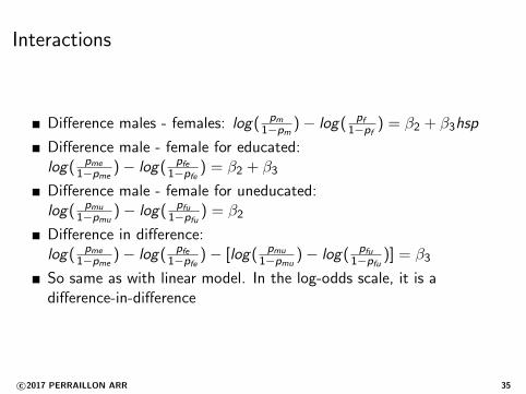
Difference males - females: log( pm1−pm
) − log( pf1−pf
) = β2 + β3hsp
Difference male - female for educated:log( pme
1−pme) − log( pfe
1−pfe) = β2 + β3
Difference male - female for uneducated:log( pmu
1−pmu) − log( pfu
1−pfu) = β2
Difference in difference:log( pme
1−pme) − log( pfe
1−pfe) − [log( pmu
1−pmu) − log( pfu
1−pfu)] = β3
So same as with linear model. In the log-odds scale, it is adifference-in-difference
c©2017 PERRAILLON ARR 35
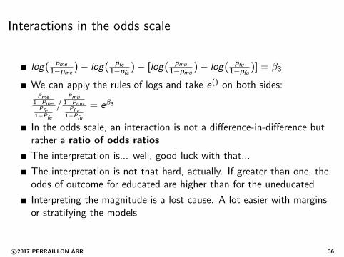
Interactions in the odds scale
log( pme
1−pme) − log( pfe
1−pfe) − [log( pmu
1−pmu) − log( pfu
1−pfu)] = β3
We can apply the rules of logs and take e() on both sides:Pme
1−PmePfe
1−Pfe
/Pmu
1−PmuPfu
1−Pfu
= eβ3
In the odds scale, an interaction is not a difference-in-difference butrather a ratio of odds ratios
The interpretation is... well, good luck with that...
The interpretation is not that hard, actually. If greater than one, theodds of outcome for educated are higher than for the uneducated
Interpreting the magnitude is a lost cause. A lot easier with marginsor stratifying the models
c©2017 PERRAILLON ARR 36
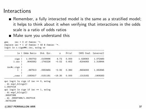
Interactions
Remember, a fully interacted model is the same as a stratified model;it helps to think about it when verifying that interactions in the oddsscale is a ratio of odds ratios
Make sure you understand this
gen inc = 0 if faminc ~=.
replace inc = 1 if faminc > 40 & faminc ~=.
logit lw c.cigs##i.inc, nolog or
------------------------------------------------------------------------------
lw | Odds Ratio Std. Err. z P>|z| [95% Conf. Interval]
-------------+----------------------------------------------------------------
cigs | 1.050702 .0109996 4.72 0.000 1.029363 1.072483
1.inc | .9045562 .1740226 -0.52 0.602 .6204083 1.318844
|
inc#c.cigs |
1 | .947913 .0553484 -0.92 0.360 .8454093 1.062845
|
_cons | .1583417 .0151181 -19.30 0.000 .1313182 .1909263
------------------------------------------------------------------------------
qui logit lw cigs if inc == 0, nolog
. di exp(_b[cigs])
1.0507018
qui logit lw cigs if inc == 1, nolog
. di exp(_b[cigs])
.99597388
. di .99597388/1.0507018
.94791299
c©2017 PERRAILLON ARR 37
Digression
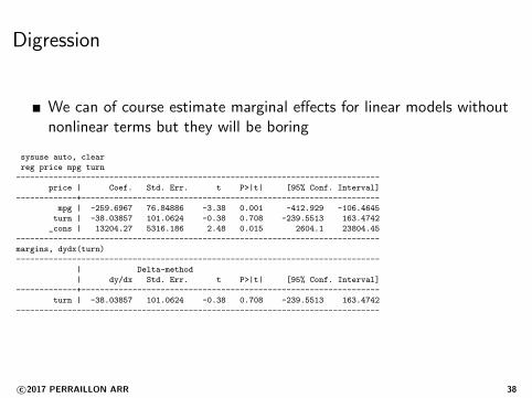
We can of course estimate marginal effects for linear models withoutnonlinear terms but they will be boring
sysuse auto, clear
reg price mpg turn
------------------------------------------------------------------------------
price | Coef. Std. Err. t P>|t| [95% Conf. Interval]
-------------+----------------------------------------------------------------
mpg | -259.6967 76.84886 -3.38 0.001 -412.929 -106.4645
turn | -38.03857 101.0624 -0.38 0.708 -239.5513 163.4742
_cons | 13204.27 5316.186 2.48 0.015 2604.1 23804.45
------------------------------------------------------------------------------
margins, dydx(turn)
------------------------------------------------------------------------------
| Delta-method
| dy/dx Std. Err. t P>|t| [95% Conf. Interval]
-------------+----------------------------------------------------------------
turn | -38.03857 101.0624 -0.38 0.708 -239.5513 163.4742
------------------------------------------------------------------------------
c©2017 PERRAILLON ARR 38
Margins are predictions
The essence of margins and marginal effects is that they arepredictions
We are using our estimated model to make predictions when wechange a continuous variable by a small amount or when we changean indicator variable from 0 to 1
They are extremely useful because they allow us to interpret ourmodels
They are truly indispensable when the scale of estimation is not thesame as the scale of interest (logit, Poisson, etc) or when we havenon-linear terms
Now we will see more about predictions in logistic models
c©2017 PERRAILLON ARR 39
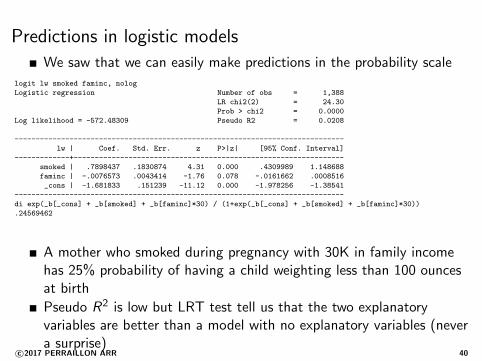
Predictions in logistic models
We saw that we can easily make predictions in the probability scale
logit lw smoked faminc, nolog
Logistic regression Number of obs = 1,388
LR chi2(2) = 24.30
Prob > chi2 = 0.0000
Log likelihood = -572.48309 Pseudo R2 = 0.0208
------------------------------------------------------------------------------
lw | Coef. Std. Err. z P>|z| [95% Conf. Interval]
-------------+----------------------------------------------------------------
smoked | .7898437 .1830874 4.31 0.000 .4309989 1.148688
faminc | -.0076573 .0043414 -1.76 0.078 -.0161662 .0008516
_cons | -1.681833 .151239 -11.12 0.000 -1.978256 -1.38541
------------------------------------------------------------------------------
di exp(_b[_cons] + _b[smoked] + _b[faminc]*30) / (1+exp(_b[_cons] + _b[smoked] + _b[faminc]*30))
.24569462
A mother who smoked during pregnancy with 30K in family incomehas 25% probability of having a child weighting less than 100 ouncesat birth
Pseudo R2 is low but LRT test tell us that the two explanatoryvariables are better than a model with no explanatory variables (nevera surprise)
c©2017 PERRAILLON ARR 40

Predictions in logistic models
One way to evaluate the predictive ability of our models is to comparepredictors and observed values
We did so with linear models. We can use the root mean square error(RMSE) or the R2 because it is also the square of the correlationbetween observed and predicted values
In logistic models, the observed value is a 1/0 variable but predictedvalues are either in the log odds scale or in the probability scale
We can transform probabilities into 1/0 values. If the predictedprobabilities is ≥ 0.5, then that means that the observation is morelikely than not to experience the event
c©2017 PERRAILLON ARR 41
Correctly predicted
One way to evaluate the predictive ability of our models is to comparepredictors and observed values
We did so with linear models. We can use the root mean square error(RMSE) or the R2 because it is also the square of the correlationbetween observed and predicted values
In logistic models, the observed value is a 1/0 variable but predictedvalues are either in the log odds scale or in the probability scale
We can transform probabilities into 1/0 values. If the predictedprobabilities is ≥ 0.5, then that means that the observation is morelikely than not to experience the event
c©2017 PERRAILLON ARR 42

Correctly predicted
Calculating the observations correctly predicted
qui logit lw smoked faminc, nolog
predict phat if e(sample)
gen hatlw = 0 if phat ~= .
replace hatlw = 1 if phat >= 0.5 & phat ~= .
tab lw hatlw, row col
tab lw hatlw
| hatlw
lw | 0 | Total
-----------+-----------+----------
0 | 1,180 | 1,180
1 | 207 | 207
-----------+-----------+----------
Total | 1,387 | 1,387
But... low birth weight is not that common so using 0.5 as the cut offpoint doesn’t make much sense
c©2017 PERRAILLON ARR 43
Remembering epi
From Wiki:
Sensitivity: True positive; proportion of positives that are correctlyidentified as such (i.e. the percentage of sick people who are correctlyidentified as having the condition).
Specificity: True negative; proportion of negatives that are correctlyidentified as such (i.e., the percentage of healthy people who arecorrectly identified as not having the condition).
False positive: 1-specificity
Sensitivity and specificity are both correct predictions, either positive(1) or negative (0)
We can just focus on whether we get the 1s right. We will usetrue positives (sensitivity) and false positives (1-specificity)
c©2017 PERRAILLON ARR 44
Calculating sensitivity and specificity
We need to come up with a cut-off point; we saw that if the cut-offpoint is 0.5 our rate of false positives (1-specificity) is 1 because wedon’t classify anybody as 1
If we lower the cut-off too much, everybody will be a one: our modelis too sensitive but not specific
Of course, there is a command for that and graph: thepost-estimation command lsens
c©2017 PERRAILLON ARR 45
Sensitivity and specificity
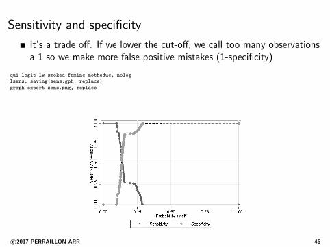
It’s a trade off. If we lower the cut-off, we call too many observationsa 1 so we make more false positive mistakes (1-specificity)
qui logit lw smoked faminc motheduc, nolog
lsens, saving(sens.gph, replace)
graph export sens.png, replace
c©2017 PERRAILLON ARR 46
How can we evaluate predictions?
Remember, the outcome is a 1/0 variable. If we just try to guessrandomly, we have 50/50 change to get it right
So our model should be at least better than chance
One way to calculate and graph this is by using the ReceiverOperating Characteristic (ROC) (has its origins in signal detectiontheory
Essentially, it plots sensitivity and 1-specificity (true positives, falsepositives) using different cut-off points to determine if the observationis a 1 (going from cut-off point 0 to 1)
The area under the curve is a measure of how good is the model atdiscriminating 1s
It also called c-statistic or concordance statistic (higher is better)
c©2017 PERRAILLON ARR 47
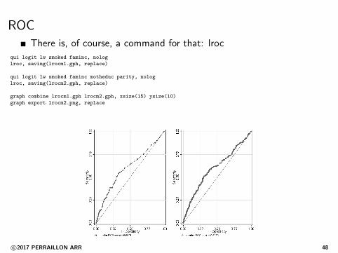
ROCThere is, of course, a command for that: lroc
qui logit lw smoked faminc, nolog
lroc, saving(lrocm1.gph, replace)
qui logit lw smoked faminc motheduc parity, nolog
lroc, saving(lrocm2.gph, replace)
graph combine lrocm1.gph lrocm2.gph, xsize(15) ysize(10)
graph export lrocm2.png, replace
c©2017 PERRAILLON ARR 48
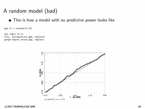
A random model (bad)
This is how a model with no predictive power looks like
gen x1 = rnormal(0,10)
qui logit lw x1
lroc, saving(noise.gph, replace)
graph export noise.png, replace
c©2017 PERRAILLON ARR 49
What happened?
In our linear model, adding more variables was always better (R2
won’t go down)
When you are in the world of models in which the mean alsodetermines the variance, adding more variables is not always better
We just made the model worse: area under the curve went from 0.6to 0.59. Not terrible, but adding more variables was not better
Parsimony in these models is a good thing and we must be carefulabout adding unnecessary variables
c©2017 PERRAILLON ARR 50

Summary
Main difficulty with logistic models is to interpret parameters
Marginal effects come to the rescue
Different terms for these types of effects. AMEs are usually calledaverage predicted comparisons
What we did today was about PREDICTION, 100 percent. We usepredictions to understand what our models are saying
The existence of the margins command has unified some of theterminology
But if you talk to your friendly statistician, you need to explainwhat you mean by marginal effects. They start thinking aboutintegrals in their heads when we mean derivatives...
c©2017 PERRAILLON ARR 51