wavelet toolbox™ 4 - luleå university of technology/wavelet toolbox 4 user's guide... ·...

Wavelet Toolbox™ 4User’s Guide

Michel MisitiYves MisitiGeorges OppenheimJean-Michel Poggi

How to Contact The MathWorks:

www.mathworks.com Webcomp.soft-sys.matlab Newsgroup www.mathworks.com/contact_TS.html Technical support

[email protected] Product enhancement suggestions [email protected] Bug reports [email protected] Documentation error reports [email protected] Order status, license renewals, [email protected] Sales, pricing, and general information

508-647-7000 (Phone)

508-647-7001 (Fax)

The MathWorks, Inc.3 Apple Hill DriveNatick, MA 01760-2098

For contact information about worldwide offices, see the MathWorks Web site.

Wavelet Toolbox™ User’s Guide © COPYRIGHT 1997–2009 by The MathWorks, Inc. The software described in this document is furnished under a license agreement. The software may be used or copied only under the terms of the license agreement. No part of this manual may be photocopied or repro-duced in any form without prior written consent from The MathWorks, Inc.

FEDERAL ACQUISITION: This provision applies to all acquisitions of the Program and Documentation by, for, or through the federal government of the United States. By accepting delivery of the Program or Documentation, the government hereby agrees that this software or documentation qualifies as commercial computer software or commercial computer software documentation as such terms are used or defined in FAR 12.212, DFARS Part 227.72, and DFARS 252.227-7014. Accordingly, the terms and conditions of this Agreement and only those rights specified in this Agreement, shall pertain to and govern the use, modification, reproduction, release, performance, display, and disclosure of the Program and Documentation by the federal government (or other entity acquiring for or through the federal government) and shall supersede any conflicting contractual terms or conditions. If this License fails to meet the government's needs or is inconsistent in any respect with federal procurement law, the government agrees to return the Program and Documentation, unused, to The MathWorks, Inc.

TrademarksMATLAB and Simulink are registered trademarks of The MathWorks, Inc. See www.mathworks.com/trademarks for a list of additional trademarks. Other product or brand names may be trademarks or registered trademarks of their respective holders.

PatentsThe MathWorks products are protected by one or more U.S. patents. Please see www.mathworks.com/patents for more information.

Revision History

March 1997 First printing New for Version 1.0September 2000 Second printing Revised for Version 2.0 (Release 12)June 2001 Online only Revised for Version 2.1 (Release 12.1)July 2002 Online only Revised for Version 2.2 (Release 13)June 2004 Online only Revised for Version 3.0 (Release 14)July 2004 Third printing Revised for Version 3.0October 2004 Online only Revised for Version 3.0.1 (Release 14SP1)March 2005 Online only Revised for Version 3.0.2 (Release 14SP2)June 2005 Fourth printing Minor revision for Version 3.0.2September 2005 Online only Minor revision for Version 3.0.3 (Release R14SP3)March 2006 Online only Minor revision for Version 3.0.4 (Release 2006a)September 2006 Online only Revised for Version 3.1 (Release 2006b)March 2007 Online only Revised for Version 4.0 (Release 2007a)September 2007 Online only Revised for Version 4.1 (Release 2007b)October 2007 Fifth printing Revised for Version 4.1March 2008 Online only Revised for Version 4.2 (Release 2008a)October 2008 Online only Revised for Version 4.3 (Release 2008b)March 2009 Online only Revised for Version 4.4 (Release 2009a)September 2009 Online only Minor revision for Version 4.4.1 (Release 2009b)

AcknowledgmentsThe authors wish to express their gratitude to all the colleagues who directly or indirectly contributed to the making of the Wavelet Toolbox™ software.

Specifically

• For the wavelet questions to Pierre-Gilles Lemarié-Rieusset (Evry) and Yves Meyer (ENS Cachan)

• For the statistical questions to Lucien Birgé (Paris 6), Pascal Massart (Paris 11) and Marc Lavielle (Paris 5)

• To David Donoho (Stanford) and to Anestis Antoniadis (Grenoble), who give generously so many valuable ideas

Colleagues and friends who have helped us steadily are Patrice Abry (ENS Lyon), Samir Akkouche (Ecole Centrale de Lyon), Mark Asch (Paris 11), Patrice Assouad (Paris 11), Roger Astier (Paris 11), Jean Coursol (Paris 11), Didier Dacunha-Castelle (Paris 11), Claude Deniau (Marseille), Patrick Flandrin (Ecole Normale de Lyon), Eric Galin (Ecole Centrale de Lyon), Christine Graffigne (Paris 5), Anatoli Juditsky (Grenoble), Gérard Kerkyacharian (Paris 10), Gérard Malgouyres (Paris 11), Olivier Nowak (Ecole Centrale de Lyon), Dominique Picard (Paris 7), and Franck Tarpin-Bernard (Ecole Centrale de Lyon).

Several student groups have tested preliminary versions.

One of our first opportunities to apply the ideas of wavelets connected with signal analysis and its modeling occurred during a close and pleasant cooperation with the team “Analysis and Forecast of the Electrical Consumption” of Electricité de France (Clamart-Paris) directed first by Jean-Pierre Desbrosses, and then by Hervé Laffaye, and which included Xavier Brossat, Yves Deville, and Marie-Madeleine Martin.

Many thanks to those who tested and helped to refine the software and the printed matter and at last to The MathWorks group and specially to Roy Lurie, Jim Tung, Bruce Sesnovich, Jad Succari, Jane Carmody, and Paul Costa.

And finally, apologies to those we may have omitted.

About the Authors

Michel Misiti, Georges Oppenheim, and Jean-Michel Poggi are mathematics professors at Ecole Centrale de Lyon, University of Marne-La-Vallée and Paris 5 University. Yves Misiti is a research engineer specializing in Computer Sciences at Paris 11 University.

The authors are members of the “Laboratoire de Mathématique” at Orsay-Paris 11 University France. Their fields of interest are statistical signal processing, stochastic processes, adaptive control, and wavelets. The authors’ group, established more than 15 years ago, has published numerous theoretical papers and carried out applications in close collaboration with industrial teams. For instance:

• Robustness of the piloting law for a civilian space launcher for which an expert system was developed

• Forecasting of the electricity consumption by nonlinear methods

• Forecasting of air pollution

Notes by Yves Meyer

The history of wavelets is not very old, at most 10 to 15 years. The field experienced a fast and impressive start, characterized by a close-knit international community of researchers who freely circulated scientific information and were driven by the researchers’ youthful enthusiasm. Even as the commercial rewards promised to be significant, the ideas were shared, the trials were pooled together, and the successes were shared by the community.

There are lots of successes for the community to share. Why? Probably because the time is ripe. Fourier techniques were liberated by the appearance of windowed Fourier methods that operate locally on a time-frequency approach. In another direction, Burt-Adelson’s pyramidal algorithms, the quadrature mirror filters, and filter banks and subband coding are available. The mathematics underlying those algorithms existed earlier, but new computing techniques enabled researchers to try out new ideas rapidly. The numerical image and signal processing areas are blooming.

The wavelets bring their own strong benefits to that environment: a local outlook, a multiscaled outlook, cooperation between scales, and a time-scale analysis. They demonstrate that sines and cosines are not the only useful

functions and that other bases made of weird functions serve to look at new foreign signals, as strange as most fractals or some transient signals.

Recently, wavelets were determined to be the best way to compress a huge library of fingerprints. This is not only a milestone that highlights the practical value of wavelets, but it has also proven to be an instructive process for the researchers involved in the project. Our initial intuition generally was that the proper way to tackle this problem of interweaving lines and textures was to use wavelet packets, a flexible technique endowed with quite a subtle sharpness of analysis and a substantial compression capability. However, it was a biorthogonal wavelet that emerged victorious and at this time represents the best method in terms of cost as well as speed. Our intuitions led one way, but implementing the methods settled the issue by pointing us in the right direction.

For wavelets, the period of growth and intuition is becoming a time of consolidation and implementation. In this context, a toolbox is not only possible, but valuable. It provides a working environment that permits experimentation and enables implementation.

Since the field still grows, it has to be vast and open. The Wavelet Toolbox product addresses this need, offering an array of tools that can be organized according to several criteria:

• Synthesis and analysis tools

• Wavelet and wavelet packets approaches

• Signal and image processing

• Discrete and continuous analyses

• Orthogonal and redundant approaches

• Coding, de-noising and compression approaches

What can we anticipate for the future, at least in the short term? It is difficult to make an accurate forecast. Nonetheless, it is reasonable to think that the pace of development and experimentation will carry on in many different fields. Numerical analysis constantly uses new bases of functions to encode its operators or to simplify its calculations to solve partial differential equations. The analysis and synthesis of complex transient signals touches musical instruments by studying the striking up, when the bow meets the cello string. The analysis and synthesis of multifractal signals, whose regularity (or rather irregularity) varies with time, localizes information of interest at its

geographic location. Compression is a booming field, and coding and de-noising are promising.

For each of these areas, the Wavelet Toolbox software provides a way to introduce, learn, and apply the methods, regardless of the user’s experience. It includes a command-line mode and a graphical user interface mode, each very capable and complementing to the other. The user interfaces help the novice to get started and the expert to implement trials. The command line provides an open environment for experimentation and addition to the graphical interface.

In the journey to the heart of a signal’s meaning, the toolbox gives the traveler both guidance and freedom: going from one point to the other, wandering from a tree structure to a superimposed mode, jumping from low to high scale, and skipping a breakdown point to spot a quadratic chirp. The time-scale graphs of continuous analysis are often breathtaking and more often than not enlightening as to the structure of the signal.

Here are the tools, waiting to be used.

Yves MeyerProfessor, Ecole Normale Supérieure de Cachan and Institut de France

Notes by Ingrid Daubechies

Wavelet transforms, in their different guises, have come to be accepted as a set of tools useful for various applications. Wavelet transforms are good to have at one’s fingertips, along with many other mostly more traditional tools.

Wavelet Toolbox software is a great way to work with wavelets. The toolbox, together with the power of MATLAB® software, really allows one to write complex and powerful applications, in a very short amount of time. The Graphic User Interface is both user-friendly and intuitive. It provides an excellent interface to explore the various aspects and applications of wavelets; it takes away the tedium of typing and remembering the various function calls.

Ingrid C. DaubechiesProfessor, Princeton University, Department of Mathematics and Program in Applied and Computational Mathematics

1 Wavelets: A New Tool for Signal Analysis

1-2

Product OverviewEverywhere around us are signals that can be analyzed. For example, there are seismic tremors, human speech, engine vibrations, medical images, financial data, music, and many other types of signals. Wavelet analysis is a new and promising set of tools and techniques for analyzing these signals.

Wavelet Toolbox™ software is a collection of functions built on the MATLAB® technical computing environment. It provides tools for the analysis and synthesis of signals and images, and tools for statistical applications, using wavelets and wavelet packets within the framework of MATLAB.

The MathWorks™ provides several products that are relevant to the kinds of tasks you can perform with the toolbox. For more information about any of these products, see the products section of The MathWorks Web site.

Wavelet Toolbox software provides two categories of tools:

• Command-line functions

• Graphical interactive tools

The first category of tools is made up of functions that you can call directly from the command line or from your own applications. Most of these functions are M-files, series of statements that implement specialized wavelet analysis or synthesis algorithms. You can view the code for these functions using the following statement:

type function_name

You can view the header of the function, the help part, using the statement

help function_name

A summary list of the Wavelet Toolbox functions is available to you by typing

help wavelet

You can change the way any toolbox function works by copying and renaming the M-file, then modifying your copy. You can also extend the toolbox by adding your own M-files.

Product Overview

1-3

The second category of tools is a collection of graphical interface tools that afford access to extensive functionality. Access these tools from the command line by typing

wavemenu

Note The examples in this guide are generated using Wavelet Toolbox software with the DWT extension mode set to 'zpd' (for zero padding), except when it is explicitly mentioned. So if you want to obtain exactly the same numerical results, type dwtmode('zpd'), before to execute the example code.

In most of the command-line examples, figures are displayed. To clarify the presentation, the plotting commands are partially or completely omitted. To reproduce the displayed figures exactly, you would need to insert some graphical commands in the example code.


1-4

Background ReadingWavelet Toolbox™ software provides a complete introduction to wavelets and assumes no previous knowledge of the area. The toolbox allows you to use wavelet techniques on your own data immediately and develop new insights.

It is our hope that, through the use of these practical tools, you may want to explore the beautiful underlying mathematics and theory.

Excellent supplementary texts provide complementary treatments of wavelet theory and practice (see “References” on page 6-155). For instance:

• Burke-Hubbard [Bur96] is an historical and up-to-date text presenting the concepts using everyday words.

• Daubechies [Dau92] is a classic for the mathematics.

• Kaiser [Kai94] is a mathematical tutorial, and a physics-oriented book.

• Mallat [Mal98] is a 1998 book, which includes recent developments, and consequently is one of the most complete.

• Meyer [Mey93] is the “father” of the wavelet books.

• Strang-Nguyen [StrN96] is especially useful for signal processing engineers. It offers a clear and easy-to-understand introduction to two central ideas: filter banks for discrete signals, and for wavelets. It fully explains the connection between the two. Many exercises in the book are drawn from Wavelet Toolbox software.

The Wavelet Digest Internet site (http://www.wavelet.org/) provides much useful and practical information.

Installing Wavelet Toolbox™ Software

1-5

Installing Wavelet Toolbox™ SoftwareTo install this toolbox on your computer, see the appropriate platform-specific MATLAB® installation guide. To determine if the Wavelet Toolbox™ software is already installed on your system, check for a subdirectory named wavelet within the main toolbox directory or folder.

Wavelet Toolbox software can perform signal or image analysis. For indexed images or truecolor images (represented by m-by-n-by-3 arrays of uint8), all wavelet functions use floating-point operations. To avoid Out of Memory errors, be sure to allocate enough memory to process various image sizes.

The memory can be real RAM or can be a combination of RAM and virtual memory. See your operating system documentation for how to configure virtual memory.

System RecommendationsWhile not a requirement, we recommend you obtain Signal Processing Toolbox™ and Image Processing Toolbox™ software to use in conjunction with the Wavelet Toolbox software. These toolboxes provide complementary functionality that give you maximum flexibility in analyzing and processing signals and images.

This manual makes no assumption that your computer is running any other MATLAB toolboxes.

Platform-Specific DetailsSome details of the use of the Wavelet Toolbox software may depend on your hardware or operating system.

Windows FontsWe recommend you set your operating system to use “Small Fonts.” Set this option by clicking the Display icon in your desktop’s Control Panel (accessible through the Settings�Control Panel submenu). Select the Configuration option, and then use the Font Size menu to change to Small Fonts. You’ll have to restart Windows® for this change to take effect.


1-6

Fonts for Non-Windows PlatformsWe recommend you set your operating system to use standard default fonts.

However, for all platforms, if you prefer to use large fonts, some of the labels in the GUI figures may be illegible when using the default display mode of the toolbox. To change the default mode to accept large fonts, use the wtbxmngr function. (For more information, see either the wtbxmngr help or its reference page.)

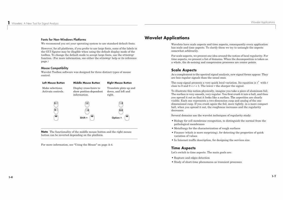
Mouse CompatibilityWavelet Toolbox software was designed for three distinct types of mouse control.

Note The functionality of the middle mouse button and the right mouse button can be inverted depending on the platform.

For more information, see “Using the Mouse” on page A-4.

Left Mouse Button Middle Mouse Button Right Mouse Button

Make selections. Activate controls.

Display cross-hairs to show position-dependent information.

Translate plots up and down, and left and right.

Shift + Option +

Wavelet Applications

1-7

Wavelet ApplicationsWavelets have scale aspects and time aspects, consequently every application has scale and time aspects. To clarify them we try to untangle the aspects somewhat arbitrarily.

For scale aspects, we present one idea around the notion of local regularity. For time aspects, we present a list of domains. When the decomposition is taken as a whole, the de-noising and compression processes are center points.

Scale AspectsAs a complement to the spectral signal analysis, new signal forms appear. They are less regular signals than the usual ones.

The cusp signal presents a very quick local variation. Its equation is with t close to 0 and 0 < r < 1. The lower r the sharper the signal.

To illustrate this notion physically, imagine you take a piece of aluminum foil; The surface is very smooth, very regular. You first crush it into a ball, and then you spread it out so that it looks like a surface. The asperities are clearly visible. Each one represents a two-dimension cusp and analog of the one dimensional cusp. If you crush again the foil, more tightly, in a more compact ball, when you spread it out, the roughness increases and the regularity decreases.

Several domains use the wavelet techniques of regularity study:

• Biology for cell membrane recognition, to distinguish the normal from the pathological membranes

• Metallurgy for the characterization of rough surfaces

• Finance (which is more surprising), for detecting the properties of quick variation of values

• In Internet traffic description, for designing the services size

Time AspectsLet’s switch to time aspects. The main goals are:

• Rupture and edges detection

• Study of short-time phenomena as transient processes

tr


1-8

As domain applications, we get:

• Industrial supervision of gear-wheel

• Checking undue noises in craned or dented wheels, and more generally in nondestructive control quality processes

• Detection of short pathological events as epileptic crises or normal ones as evoked potentials in EEG (medicine)

• SAR imagery

• Automatic target recognition

• Intermittence in physics

Wavelet Decomposition as a WholeMany applications use the wavelet decomposition taken as a whole. The common goals concern the signal or image clearance and simplification, which are parts of de-noising or compression.

We find many published papers in oceanography and earth studies.

One of the most popular successes of the wavelets is the compression of FBI fingerprints.

When trying to classify the applications by domain, it is almost impossible to sum up several thousand papers written within the last 15 years. Moreover, it is difficult to get information on real-world industrial applications from companies. They understandably protect their own information.

Some domains are very productive. Medicine is one of them. We can find studies on micro-potential extraction in EKGs, on time localization of His bundle electrical heart activity, in ECG noise removal. In EEGs, a quick transitory signal is drowned in the usual one. The wavelets are able to determine if a quick signal exists, and if so, can localize it. There are attempts to enhance mammograms to discriminate tumors from calcifications.

Another prototypical application is a classification of Magnetic Resonance Spectra. The study concerns the influence of the fat we eat on our body fat. The type of feeding is the basic information and the study is intended to avoid taking a sample of the body fat. Each Fourier spectrum is encoded by some of its wavelet coefficients. A few of them are enough to code the most interesting features of the spectrum. The classification is performed on the coded vectors.

Fourier Analysis

1-9

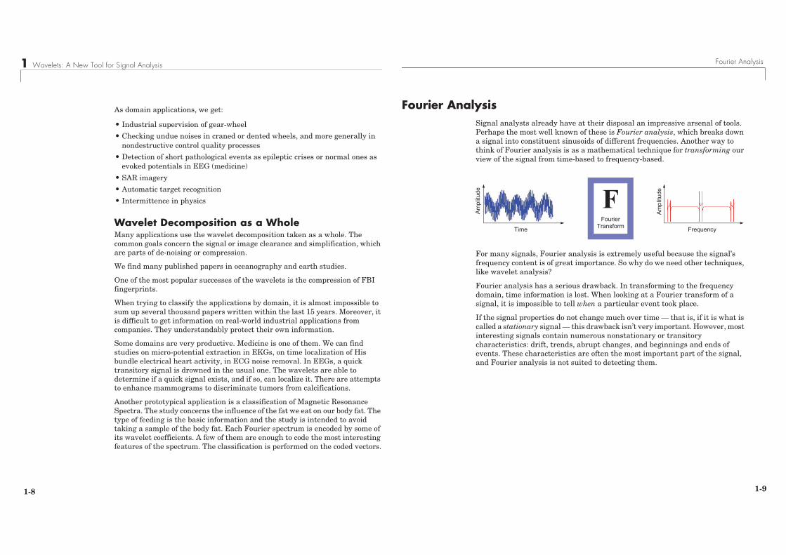
Fourier AnalysisSignal analysts already have at their disposal an impressive arsenal of tools. Perhaps the most well known of these is Fourier analysis, which breaks down a signal into constituent sinusoids of different frequencies. Another way to think of Fourier analysis is as a mathematical technique for transforming our view of the signal from time-based to frequency-based.

For many signals, Fourier analysis is extremely useful because the signal’s frequency content is of great importance. So why do we need other techniques, like wavelet analysis?

Fourier analysis has a serious drawback. In transforming to the frequency domain, time information is lost. When looking at a Fourier transform of a signal, it is impossible to tell when a particular event took place.

If the signal properties do not change much over time — that is, if it is what is called a stationary signal — this drawback isn’t very important. However, most interesting signals contain numerous nonstationary or transitory characteristics: drift, trends, abrupt changes, and beginnings and ends of events. These characteristics are often the most important part of the signal, and Fourier analysis is not suited to detecting them.

FFourier

Transform

Am

plitu

de

Time

Ampl

itude

Frequency


1-10

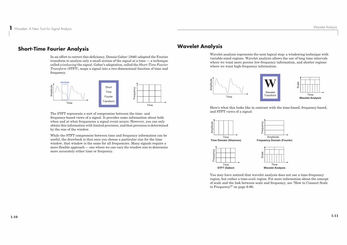
Short-Time Fourier AnalysisIn an effort to correct this deficiency, Dennis Gabor (1946) adapted the Fourier transform to analyze only a small section of the signal at a time — a technique called windowing the signal. Gabor’s adaptation, called the Short-Time Fourier Transform (STFT), maps a signal into a two-dimensional function of time and frequency.

The STFT represents a sort of compromise between the time- and frequency-based views of a signal. It provides some information about both when and at what frequencies a signal event occurs. However, you can only obtain this information with limited precision, and that precision is determined by the size of the window.

While the STFT compromise between time and frequency information can be useful, the drawback is that once you choose a particular size for the time window, that window is the same for all frequencies. Many signals require a more flexible approach — one where we can vary the window size to determine more accurately either time or frequency.

Short

Transform

Ampl

itude

TimeTime

Time

Fourier

Freq

uenc

y

window

Wavelet Analysis

1-11

Wavelet AnalysisWavelet analysis represents the next logical step: a windowing technique with variable-sized regions. Wavelet analysis allows the use of long time intervals where we want more precise low-frequency information, and shorter regions where we want high-frequency information.

Here’s what this looks like in contrast with the time-based, frequency-based, and STFT views of a signal:

You may have noticed that wavelet analysis does not use a time-frequency region, but rather a time-scale region. For more information about the concept of scale and the link between scale and frequency, see “How to Connect Scale to Frequency?” on page 6-66.

Ampl

itude

TimeTime

Scal

e

Wavelet Analysis

WWavelet

Transform

Time

Freq

uenc

y

Time

Sca

le

STFT (Gabor) Wavelet Analysis

TimeTime Domain (Shannon)

Freq

uenc

y

Frequency Domain (Fourier)Amplitude

Am

plitu

de


1-12

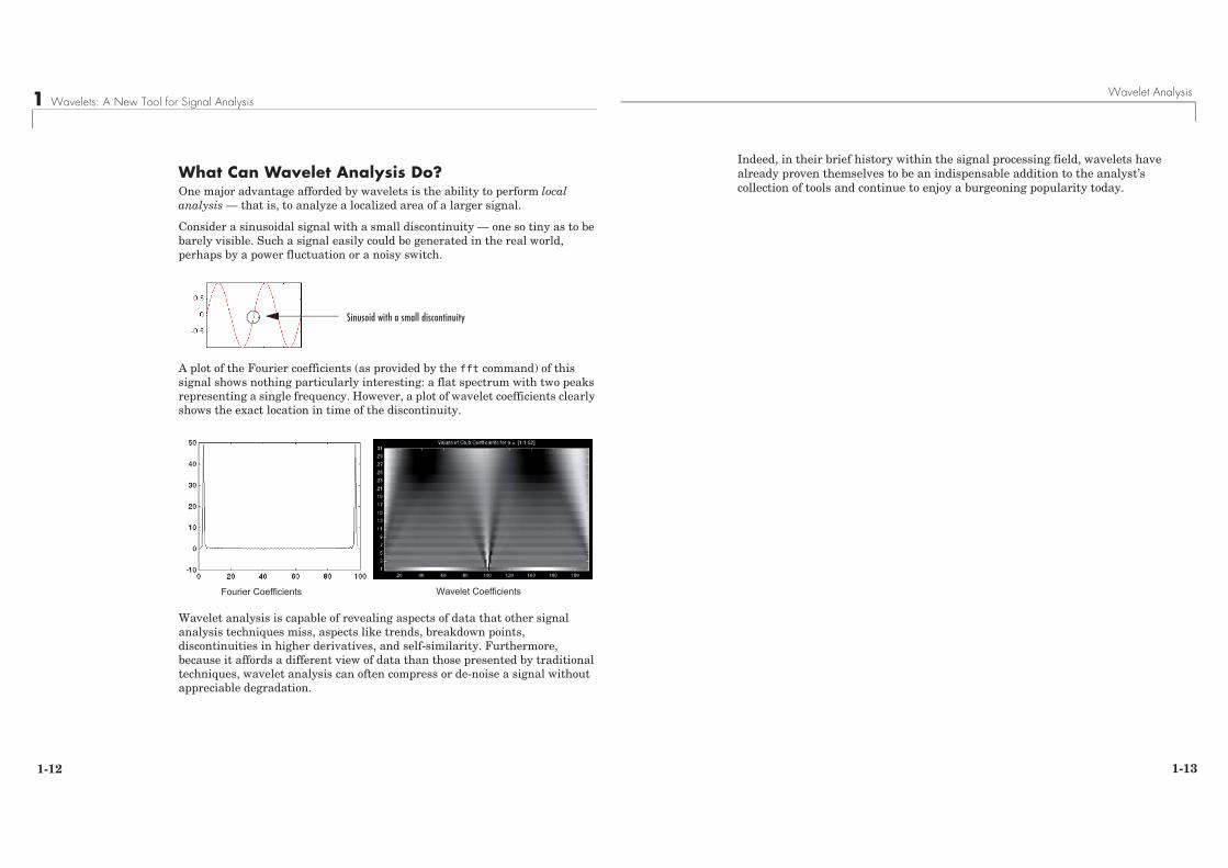
What Can Wavelet Analysis Do?One major advantage afforded by wavelets is the ability to perform local analysis — that is, to analyze a localized area of a larger signal.

Consider a sinusoidal signal with a small discontinuity — one so tiny as to be barely visible. Such a signal easily could be generated in the real world, perhaps by a power fluctuation or a noisy switch.

A plot of the Fourier coefficients (as provided by the fft command) of this signal shows nothing particularly interesting: a flat spectrum with two peaks representing a single frequency. However, a plot of wavelet coefficients clearly shows the exact location in time of the discontinuity.

Wavelet analysis is capable of revealing aspects of data that other signal analysis techniques miss, aspects like trends, breakdown points, discontinuities in higher derivatives, and self-similarity. Furthermore, because it affords a different view of data than those presented by traditional techniques, wavelet analysis can often compress or de-noise a signal without appreciable degradation.

Sinusoid with a small discontinuity

Fourier Coefficients Wavelet Coefficients

Wavelet Analysis

1-13

Indeed, in their brief history within the signal processing field, wavelets have already proven themselves to be an indispensable addition to the analyst’s collection of tools and continue to enjoy a burgeoning popularity today.


1-14

What Is Wavelet Analysis?Now that we know some situations when wavelet analysis is useful, it is worthwhile asking “What is wavelet analysis?” and even more fundamentally, “What is a wavelet?”

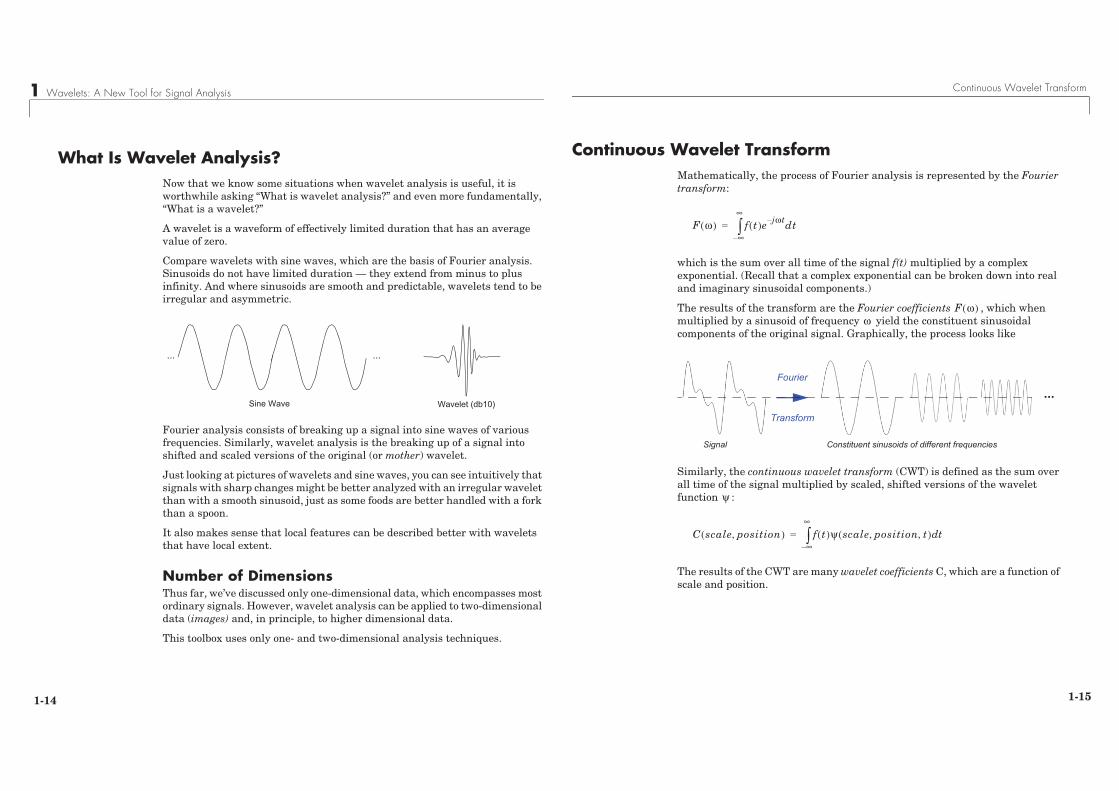
A wavelet is a waveform of effectively limited duration that has an average value of zero.

Compare wavelets with sine waves, which are the basis of Fourier analysis. Sinusoids do not have limited duration — they extend from minus to plus infinity. And where sinusoids are smooth and predictable, wavelets tend to be irregular and asymmetric.

Fourier analysis consists of breaking up a signal into sine waves of various frequencies. Similarly, wavelet analysis is the breaking up of a signal into shifted and scaled versions of the original (or mother) wavelet.

Just looking at pictures of wavelets and sine waves, you can see intuitively that signals with sharp changes might be better analyzed with an irregular wavelet than with a smooth sinusoid, just as some foods are better handled with a fork than a spoon.

It also makes sense that local features can be described better with wavelets that have local extent.

Number of DimensionsThus far, we’ve discussed only one-dimensional data, which encompasses most ordinary signals. However, wavelet analysis can be applied to two-dimensional data (images) and, in principle, to higher dimensional data.

This toolbox uses only one- and two-dimensional analysis techniques.

Sine Wave Wavelet (db10)

......

Continuous Wavelet Transform

1-15

Continuous Wavelet TransformMathematically, the process of Fourier analysis is represented by the Fourier transform:

which is the sum over all time of the signal f(t) multiplied by a complex exponential. (Recall that a complex exponential can be broken down into real and imaginary sinusoidal components.)

The results of the transform are the Fourier coefficients , which when multiplied by a sinusoid of frequency yield the constituent sinusoidal components of the original signal. Graphically, the process looks like

Similarly, the continuous wavelet transform (CWT) is defined as the sum over all time of the signal multiplied by scaled, shifted versions of the wavelet function :

The results of the CWT are many wavelet coefficients C, which are a function of scale and position.

F ω( ) f t( )e jωt–

∞–

∞

� dt=

F ω( )ω

Signal

...

Constituent sinusoids of different frequencies

Fourier

Transform

ψ

C scale position,( ) f t( )ψ scale position t,,( ) td∞–

∞

�=


1-16

Multiplying each coefficient by the appropriately scaled and shifted wavelet yields the constituent wavelets of the original signal.

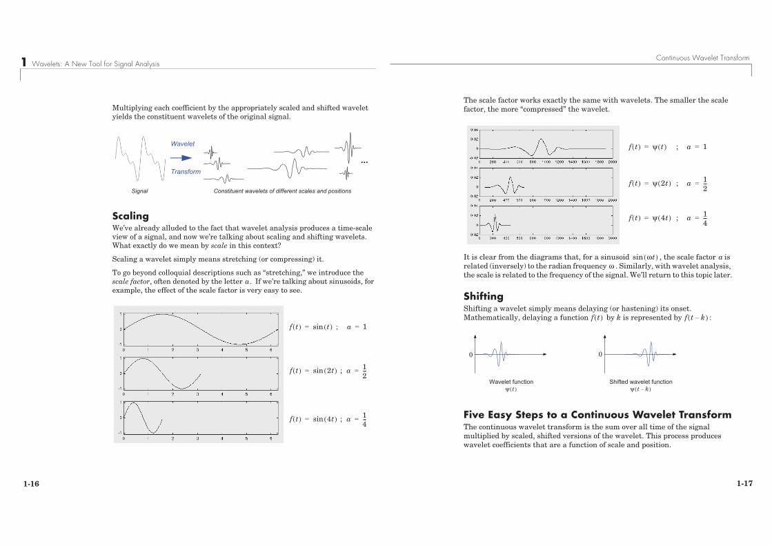
ScalingWe’ve already alluded to the fact that wavelet analysis produces a time-scale view of a signal, and now we’re talking about scaling and shifting wavelets. What exactly do we mean by scale in this context?

Scaling a wavelet simply means stretching (or compressing) it.

To go beyond colloquial descriptions such as “stretching,” we introduce the scale factor, often denoted by the letter If we’re talking about sinusoids, for example, the effect of the scale factor is very easy to see.

Signal Constituent wavelets of different scales and positions

...

Wavelet

Transform

a.

f t( ) t( )sin=

f t( ) 2t( )sin=

f t( ) 4t( )sin=

a; 1=

; a 12---=

; a 14---=


1-17

The scale factor works exactly the same with wavelets. The smaller the scale factor, the more “compressed” the wavelet.

It is clear from the diagrams that, for a sinusoid , the scale factor is related (inversely) to the radian frequency . Similarly, with wavelet analysis, the scale is related to the frequency of the signal. We’ll return to this topic later.

ShiftingShifting a wavelet simply means delaying (or hastening) its onset. Mathematically, delaying a function by k is represented by :

Five Easy Steps to a Continuous Wavelet TransformThe continuous wavelet transform is the sum over all time of the signal multiplied by scaled, shifted versions of the wavelet. This process produces wavelet coefficients that are a function of scale and position.

f t( ) ψ t( )=

f t( ) ψ 2t( )=

f t( ) ψ 4t( )=

; a 1=

; a 12---=

; a 14---=

ωt( )sin aω

f t( ) f t k–( )

Wavelet functionψ t( ) ψ t k–( )

Shifted wavelet function

0 0


1-18

It’s really a very simple process. In fact, here are the five steps of an easy recipe for creating a CWT:

1 Take a wavelet and compare it to a section at the start of the original signal.

2 Calculate a number, C, that represents how closely correlated the wavelet is with this section of the signal. The higher C is, the more the similarity. More precisely, if the signal energy and the wavelet energy are equal to one, C may be interpreted as a correlation coefficient.

Note that the results will depend on the shape of the wavelet you choose.

3 Shift the wavelet to the right and repeat steps 1 and 2 until you’ve covered the whole signal.

4 Scale (stretch) the wavelet and repeat steps 1 through 3.

Signal

Wavelet

C = 0.0102

Signal

Wavelet


1-19

5 Repeat steps 1 through 4 for all scales.

When you’re done, you’ll have the coefficients produced at different scales by different sections of the signal. The coefficients constitute the results of a regression of the original signal performed on the wavelets.

How to make sense of all these coefficients? You could make a plot on which the x-axis represents position along the signal (time), the y-axis represents scale, and the color at each x-y point represents the magnitude of the wavelet coefficient C. These are the coefficient plots generated by the graphical tools.

Signal

Wavelet

C = 0.2247

LargeCoefficients

SmallCoefficients

Sca

le

Time


1-20

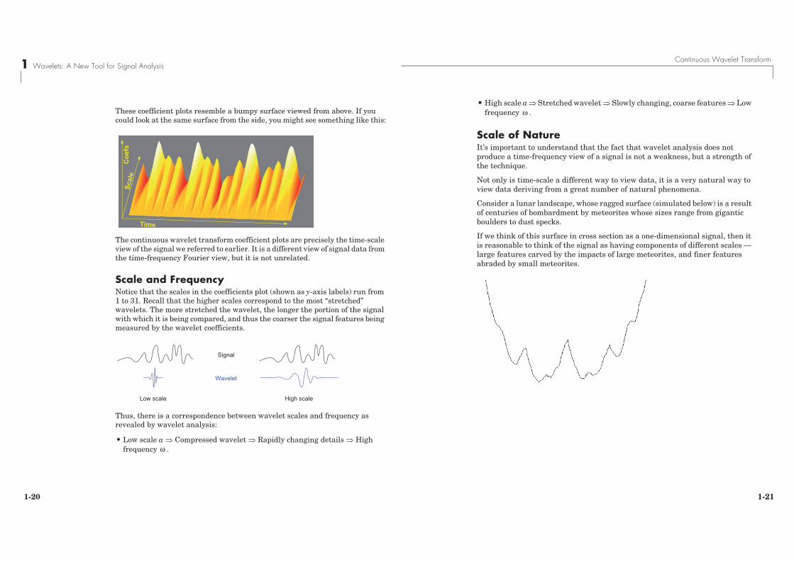
These coefficient plots resemble a bumpy surface viewed from above. If you could look at the same surface from the side, you might see something like this:

The continuous wavelet transform coefficient plots are precisely the time-scale view of the signal we referred to earlier. It is a different view of signal data from the time-frequency Fourier view, but it is not unrelated.

Scale and FrequencyNotice that the scales in the coefficients plot (shown as y-axis labels) run from 1 to 31. Recall that the higher scales correspond to the most “stretched” wavelets. The more stretched the wavelet, the longer the portion of the signal with which it is being compared, and thus the coarser the signal features being measured by the wavelet coefficients.

Thus, there is a correspondence between wavelet scales and frequency as revealed by wavelet analysis:

• Low scale a � Compressed wavelet � Rapidly changing details � High frequency .

Time

Scal

eC

oefs

Signal

Wavelet

Low scale High scale

ω


1-21

• High scale a � Stretched wavelet � Slowly changing, coarse features � Low frequency .

Scale of NatureIt’s important to understand that the fact that wavelet analysis does not produce a time-frequency view of a signal is not a weakness, but a strength of the technique.

Not only is time-scale a different way to view data, it is a very natural way to view data deriving from a great number of natural phenomena.

Consider a lunar landscape, whose ragged surface (simulated below) is a result of centuries of bombardment by meteorites whose sizes range from gigantic boulders to dust specks.

If we think of this surface in cross section as a one-dimensional signal, then it is reasonable to think of the signal as having components of different scales — large features carved by the impacts of large meteorites, and finer features abraded by small meteorites.

ω


1-22

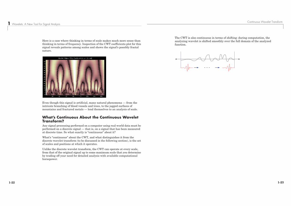
Here is a case where thinking in terms of scale makes much more sense than thinking in terms of frequency. Inspection of the CWT coefficients plot for this signal reveals patterns among scales and shows the signal’s possibly fractal nature.

Even though this signal is artificial, many natural phenomena — from the intricate branching of blood vessels and trees, to the jagged surfaces of mountains and fractured metals — lend themselves to an analysis of scale.

What’s Continuous About the Continuous WaveletTransform?Any signal processing performed on a computer using real-world data must be performed on a discrete signal — that is, on a signal that has been measured at discrete time. So what exactly is “continuous” about it?

What’s “continuous” about the CWT, and what distinguishes it from the discrete wavelet transform (to be discussed in the following section), is the set of scales and positions at which it operates.

Unlike the discrete wavelet transform, the CWT can operate at every scale, from that of the original signal up to some maximum scale that you determine by trading off your need for detailed analysis with available computational horsepower.


1-23

The CWT is also continuous in terms of shifting: during computation, the analyzing wavelet is shifted smoothly over the full domain of the analyzed function.


1-24

Discrete Wavelet TransformCalculating wavelet coefficients at every possible scale is a fair amount of work, and it generates an awful lot of data. What if we choose only a subset of scales and positions at which to make our calculations?

It turns out, rather remarkably, that if we choose scales and positions based on powers of two — so-called dyadic scales and positions — then our analysis will be much more efficient and just as accurate. We obtain such an analysis from the discrete wavelet transform (DWT). For more information on DWT, see “Algorithms” on page 6-23.

An efficient way to implement this scheme using filters was developed in 1988 by Mallat (see [Mal89] in “References” on page 6-155). The Mallat algorithm is in fact a classical scheme known in the signal processing community as a two-channel subband coder (see page 1 of the book Wavelets and Filter Banks, by Strang and Nguyen [StrN96]).

This very practical filtering algorithm yields a fast wavelet transform — a box into which a signal passes, and out of which wavelet coefficients quickly emerge. Let’s examine this in more depth.

One-Stage Filtering: Approximations and DetailsFor many signals, the low-frequency content is the most important part. It is what gives the signal its identity. The high-frequency content, on the other hand, imparts flavor or nuance. Consider the human voice. If you remove the high-frequency components, the voice sounds different, but you can still tell what’s being said. However, if you remove enough of the low-frequency components, you hear gibberish.

In wavelet analysis, we often speak of approximations and details. The approximations are the high-scale, low-frequency components of the signal. The details are the low-scale, high-frequency components.

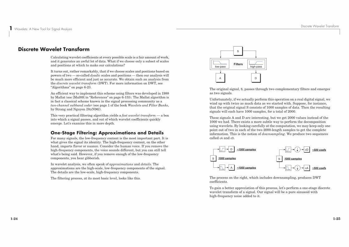
The filtering process, at its most basic level, looks like this.

Discrete Wavelet Transform

1-25

The original signal, S, passes through two complementary filters and emerges as two signals.

Unfortunately, if we actually perform this operation on a real digital signal, we wind up with twice as much data as we started with. Suppose, for instance, that the original signal S consists of 1000 samples of data. Then the resulting signals will each have 1000 samples, for a total of 2000.

These signals A and D are interesting, but we get 2000 values instead of the 1000 we had. There exists a more subtle way to perform the decomposition using wavelets. By looking carefully at the computation, we may keep only one point out of two in each of the two 2000-length samples to get the complete information. This is the notion of downsampling. We produce two sequences called cA and cD.

The process on the right, which includes downsampling, produces DWT coefficients.

To gain a better appreciation of this process, let’s perform a one-stage discrete wavelet transform of a signal. Our signal will be a pure sinusoid with high-frequency noise added to it.

S

high-pass

A D

Filterslow-pass

S

cD

cA

1000 samples

~500 coefs

~500 coefs

S

D

A

1000 samples

~1000 samples

~1000 samples


1-26

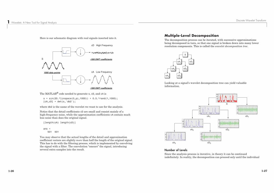
Here is our schematic diagram with real signals inserted into it.

The MATLAB® code needed to generate s, cD, and cA is

s = sin(20.*linspace(0,pi,1000)) + 0.5.*rand(1,1000);[cA,cD] = dwt(s,'db2');

where db2 is the name of the wavelet we want to use for the analysis.

Notice that the detail coefficients cD are small and consist mainly of a high-frequency noise, while the approximation coefficients cA contain much less noise than does the original signal.

[length(cA) length(cD)]

ans = 501 501

You may observe that the actual lengths of the detail and approximation coefficient vectors are slightly more than half the length of the original signal. This has to do with the filtering process, which is implemented by convolving the signal with a filter. The convolution “smears” the signal, introducing several extra samples into the result.

1000 data points

~500 DWT coefficients

~500 DWT coefficients

S

cD High Frequency

cA Low Frequency

Discrete Wavelet Transform

1-27

Multiple-Level DecompositionThe decomposition process can be iterated, with successive approximations being decomposed in turn, so that one signal is broken down into many lower resolution components. This is called the wavelet decomposition tree.

Looking at a signal’s wavelet decomposition tree can yield valuable information.

Number of LevelsSince the analysis process is iterative, in theory it can be continued indefinitely. In reality, the decomposition can proceed only until the individual

S

cA1 cD1

cA2 cD2

cA3 cD3

S

cA1 cD1

cA2 cD2

cA3 cD3


1-28

details consist of a single sample or pixel. In practice, you’ll select a suitable number of levels based on the nature of the signal, or on a suitable criterion such as entropy (see “Choosing the Optimal Decomposition” on page 6-147).

Wavelet Reconstruction

1-29

Wavelet ReconstructionWe’ve learned how the discrete wavelet transform can be used to analyze, or decompose, signals and images. This process is called decomposition or analysis. The other half of the story is how those components can be assembled back into the original signal without loss of information. This process is called reconstruction, or synthesis. The mathematical manipulation that effects synthesis is called the inverse discrete wavelet transform (IDWT).

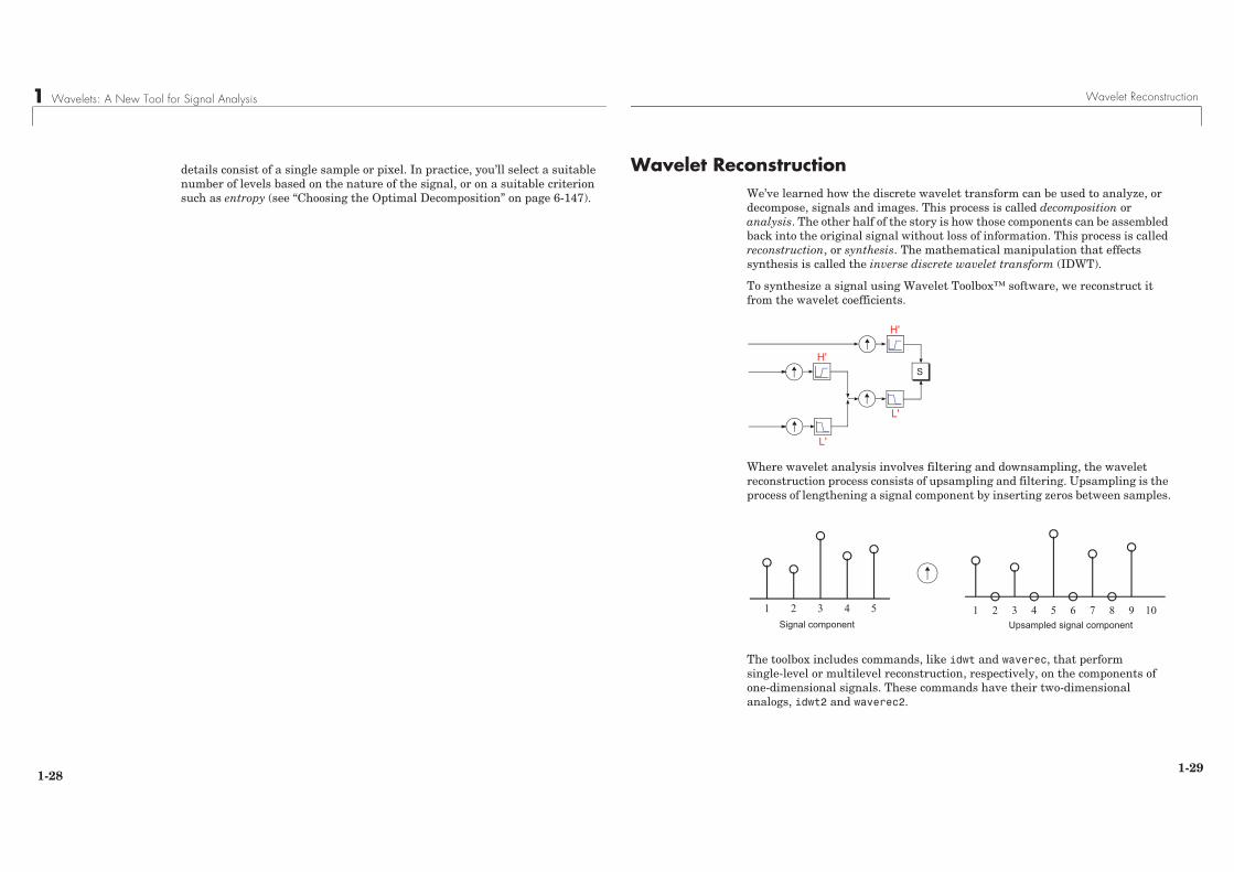
To synthesize a signal using Wavelet Toolbox™ software, we reconstruct it from the wavelet coefficients.

Where wavelet analysis involves filtering and downsampling, the wavelet reconstruction process consists of upsampling and filtering. Upsampling is the process of lengthening a signal component by inserting zeros between samples.

The toolbox includes commands, like idwt and waverec, that perform single-level or multilevel reconstruction, respectively, on the components of one-dimensional signals. These commands have their two-dimensional analogs, idwt2 and waverec2.

SH'

L'

H'

L'

Signal component Upsampled signal component

1 2 3 4 5 1 2 3 4 5 6 7 8 9 10


1-30

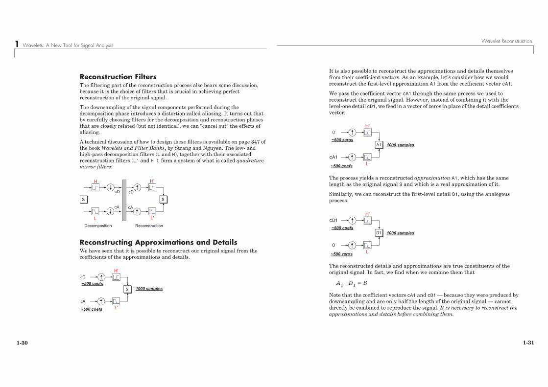
Reconstruction FiltersThe filtering part of the reconstruction process also bears some discussion, because it is the choice of filters that is crucial in achieving perfect reconstruction of the original signal.

The downsampling of the signal components performed during the decomposition phase introduces a distortion called aliasing. It turns out that by carefully choosing filters for the decomposition and reconstruction phases that are closely related (but not identical), we can “cancel out” the effects of aliasing.

A technical discussion of how to design these filters is available on page 347 of the book Wavelets and Filter Banks, by Strang and Nguyen. The low- and high-pass decomposition filters (L and H), together with their associated reconstruction filters (L' and H'), form a system of what is called quadrature mirror filters:

Reconstructing Approximations and DetailsWe have seen that it is possible to reconstruct our original signal from the coefficients of the approximations and details.

S S

Decomposition Reconstruction

H

L

H'

L'

cD

cA

cD

cA

S

H'

L'

cD

cA

1000 samples~500 coefs

~500 coefs


1-31

It is also possible to reconstruct the approximations and details themselves from their coefficient vectors. As an example, let’s consider how we would reconstruct the first-level approximation A1 from the coefficient vector cA1.

We pass the coefficient vector cA1 through the same process we used to reconstruct the original signal. However, instead of combining it with the level-one detail cD1, we feed in a vector of zeros in place of the detail coefficients vector:

The process yields a reconstructed approximation A1, which has the same length as the original signal S and which is a real approximation of it.

Similarly, we can reconstruct the first-level detail D1, using the analogous process:

The reconstructed details and approximations are true constituents of the original signal. In fact, we find when we combine them that

Note that the coefficient vectors cA1 and cD1 — because they were produced by downsampling and are only half the length of the original signal — cannot directly be combined to reproduce the signal. It is necessary to reconstruct the approximations and details before combining them.

A1

H'

L'

0

cA1

1000 samples~500 zeros

~500 coefs

D1

H'

L'

cD1

0

1000 samples~500 coefs

~500 zeros

A1 D1+ S=


1-32

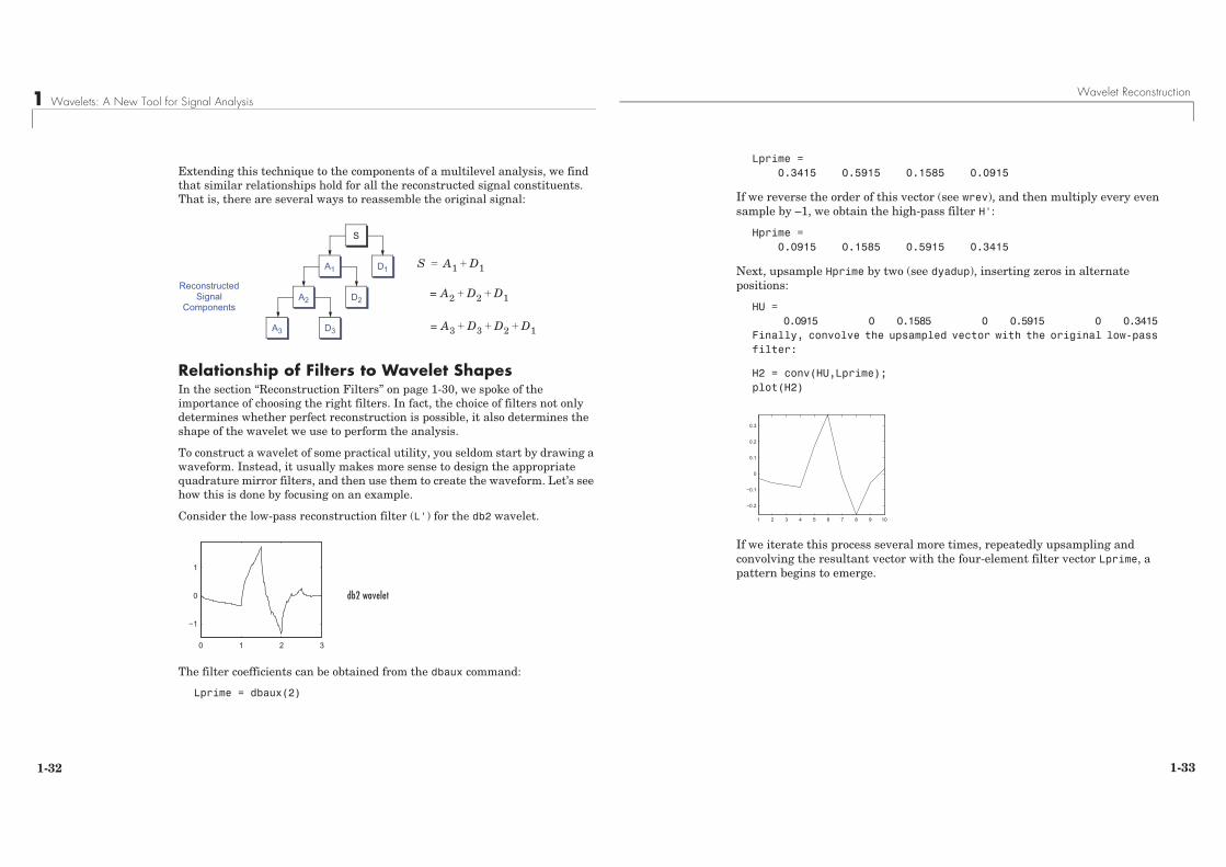
Extending this technique to the components of a multilevel analysis, we find that similar relationships hold for all the reconstructed signal constituents. That is, there are several ways to reassemble the original signal:

Relationship of Filters to Wavelet ShapesIn the section “Reconstruction Filters” on page 1-30, we spoke of the importance of choosing the right filters. In fact, the choice of filters not only determines whether perfect reconstruction is possible, it also determines the shape of the wavelet we use to perform the analysis.

To construct a wavelet of some practical utility, you seldom start by drawing a waveform. Instead, it usually makes more sense to design the appropriate quadrature mirror filters, and then use them to create the waveform. Let’s see how this is done by focusing on an example.

Consider the low-pass reconstruction filter (L') for the db2 wavelet.

The filter coefficients can be obtained from the dbaux command:

Lprime = dbaux(2)

S

A1 D1

A2 D2

A3 D3

= A2 D2 D1+ +

S A1 D1+=

= A3 D3 D2 D1+ + +

ReconstructedSignal

Components

0 1 2 3

−1

0

1

db2 wavelet


1-33

Lprime = 0.3415 0.5915 0.1585 0.0915

If we reverse the order of this vector (see wrev), and then multiply every even sample by –1, we obtain the high-pass filter H':

Hprime = 0.0915 0.1585 0.5915 0.3415

Next, upsample Hprime by two (see dyadup), inserting zeros in alternate positions:

HU = 0.0915 0 0.1585 0 0.5915 0 0.3415 Finally, convolve the upsampled vector with the original low-pass filter:

H2 = conv(HU,Lprime);plot(H2)

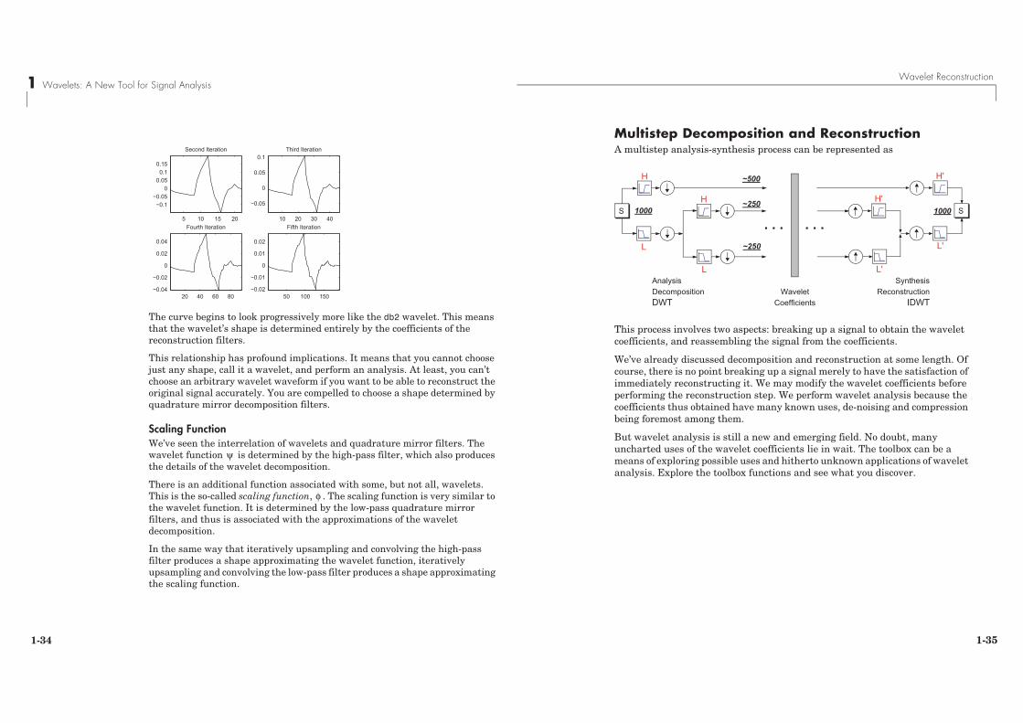
If we iterate this process several more times, repeatedly upsampling and convolving the resultant vector with the four-element filter vector Lprime, a pattern begins to emerge.

1 2 3 4 5 6 7 8 9 10

−0.2

−0.1

0

0.1

0.2

0.3


1-34

The curve begins to look progressively more like the db2 wavelet. This means that the wavelet’s shape is determined entirely by the coefficients of the reconstruction filters.

This relationship has profound implications. It means that you cannot choose just any shape, call it a wavelet, and perform an analysis. At least, you can’t choose an arbitrary wavelet waveform if you want to be able to reconstruct the original signal accurately. You are compelled to choose a shape determined by quadrature mirror decomposition filters.

Scaling FunctionWe’ve seen the interrelation of wavelets and quadrature mirror filters. The wavelet function is determined by the high-pass filter, which also produces the details of the wavelet decomposition.

There is an additional function associated with some, but not all, wavelets. This is the so-called scaling function, . The scaling function is very similar to the wavelet function. It is determined by the low-pass quadrature mirror filters, and thus is associated with the approximations of the wavelet decomposition.

In the same way that iteratively upsampling and convolving the high-pass filter produces a shape approximating the wavelet function, iteratively upsampling and convolving the low-pass filter produces a shape approximating the scaling function.

5 10 15 20

−0.1−0.05

00.050.1

0.15

Second Iteration

10 20 30 40

−0.05

0

0.05

0.1Third Iteration

20 40 60 80−0.04

−0.02

0

0.02

0.04

Fourth Iteration

50 100 150−0.02

−0.01

0

0.01

0.02

Fifth Iteration

ψ

φ


1-35

Multistep Decomposition and ReconstructionA multistep analysis-synthesis process can be represented as

This process involves two aspects: breaking up a signal to obtain the wavelet coefficients, and reassembling the signal from the coefficients.

We’ve already discussed decomposition and reconstruction at some length. Of course, there is no point breaking up a signal merely to have the satisfaction of immediately reconstructing it. We may modify the wavelet coefficients before performing the reconstruction step. We perform wavelet analysis because the coefficients thus obtained have many known uses, de-noising and compression being foremost among them.

But wavelet analysis is still a new and emerging field. No doubt, many uncharted uses of the wavelet coefficients lie in wait. The toolbox can be a means of exploring possible uses and hitherto unknown applications of wavelet analysis. Explore the toolbox functions and see what you discover.

S 1000~250

~250

S1000

~500

AnalysisDecompositionDWT

SynthesisReconstruction

IDWTWavelet

Coefficients

. . . . . .

H

L

H

L

H'

L'

H'

L'


1-38

History of WaveletsFrom an historical point of view, wavelet analysis is a new method, though its mathematical underpinnings date back to the work of Joseph Fourier in the nineteenth century. Fourier laid the foundations with his theories of frequency analysis, which proved to be enormously important and influential.

The attention of researchers gradually turned from frequency-based analysis to scale-based analysis when it started to become clear that an approach measuring average fluctuations at different scales might prove less sensitive to noise.

The first recorded mention of what we now call a “wavelet” seems to be in 1909, in a thesis by Alfred Haar.

The concept of wavelets in its present theoretical form was first proposed by Jean Morlet and the team at the Marseille Theoretical Physics Center working under Alex Grossmann in France.

The methods of wavelet analysis have been developed mainly by Y. Meyer and his colleagues, who have ensured the methods’ dissemination. The main algorithm dates back to the work of Stephane Mallat in 1988. Since then, research on wavelets has become international. Such research is particularly active in the United States, where it is spearheaded by the work of scientists such as Ingrid Daubechies, Ronald Coifman, and Victor Wickerhauser.

Barbara Burke Hubbard describes the birth, the history, and the seminal concepts in a very clear text. See The World According to Wavelets, A.K. Peters, Wellesley, 1996.

The wavelet domain is growing up very quickly. A lot of mathematical papers and practical trials are published every month.

Introduction to the Wavelet Families

1-39

Introduction to the Wavelet FamiliesSeveral families of wavelets that have proven to be especially useful are included in this toolbox. What follows is an introduction to some wavelet families.

• “Haar” on page 1-41

• “Daubechies” on page 1-42

• “Biorthogonal” on page 1-43

• “Coiflets” on page 1-45

• “Symlets” on page 1-45

• “Morlet” on page 1-46

• “Mexican Hat” on page 1-46

• “Meyer” on page 1-47

• “Other Real Wavelets” on page 1-47

• “Complex Wavelets” on page 1-47

To explore all wavelet families on your own, check out the Wavelet Display tool:

1 Type wavemenu at the MATLAB® command line. The Wavelet Toolbox Main Menu appears.


1-40

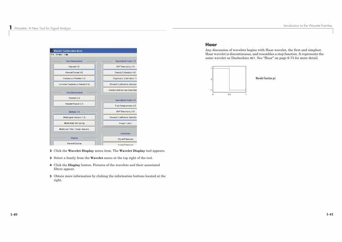
2 Click the Wavelet Display menu item. The Wavelet Display tool appears.

3 Select a family from the Wavelet menu at the top right of the tool.

4 Click the Display button. Pictures of the wavelets and their associated filters appear.

5 Obtain more information by clicking the information buttons located at the right.


1-41

HaarAny discussion of wavelets begins with Haar wavelet, the first and simplest. Haar wavelet is discontinuous, and resembles a step function. It represents the same wavelet as Daubechies db1. See “Haar” on page 6-73 for more detail.

0 0.5 1

−1

0

1

Wavelet function psi


1-42

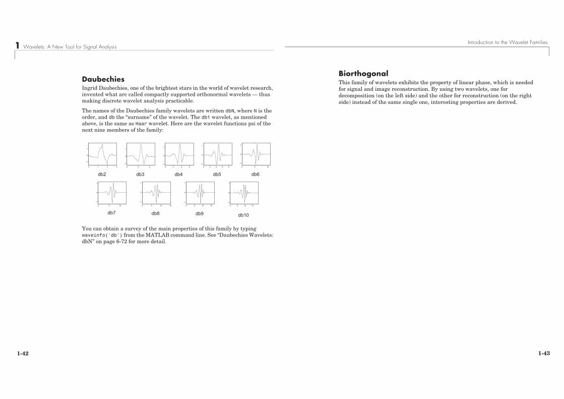
DaubechiesIngrid Daubechies, one of the brightest stars in the world of wavelet research, invented what are called compactly supported orthonormal wavelets — thus making discrete wavelet analysis practicable.

The names of the Daubechies family wavelets are written dbN, where N is the order, and db the “surname” of the wavelet. The db1 wavelet, as mentioned above, is the same as Haar wavelet. Here are the wavelet functions psi of the next nine members of the family:

You can obtain a survey of the main properties of this family by typing waveinfo('db') from the MATLAB command line. See “Daubechies Wavelets: dbN” on page 6-72 for more detail.

0 1 2 3

−1

0

1

db2 db3 db4

0 2 4

−1

0

1

0 2 4 6−1

0

1

0 2 4 6 8−1

0

1

db5 db6

0 5 10

−1

0

1

db7 db8 db9 db10

0 5 10

−1

0

1

0 5 10 15

−1

0

1

0 5 10 15

−1

0

1

0 5 10 15

−1

0

1


1-43

BiorthogonalThis family of wavelets exhibits the property of linear phase, which is needed for signal and image reconstruction. By using two wavelets, one for decomposition (on the left side) and the other for reconstruction (on the right side) instead of the same single one, interesting properties are derived.


1-44

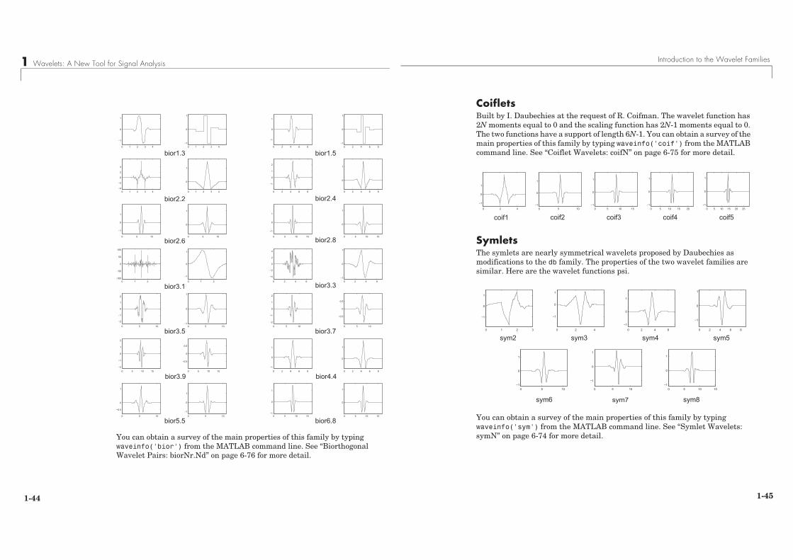
You can obtain a survey of the main properties of this family by typing waveinfo('bior') from the MATLAB command line. See “Biorthogonal Wavelet Pairs: biorNr.Nd” on page 6-76 for more detail.

0 1 2 3 4

−1

0

1

0 2 4 6 8

−1

0

1

bior1.3 bior1.50 1 2 3 4

−1

0

1

0 2 4 6 8−1

0

1

0 1 2 3 4−4

−2

0

2

4

0 2 4 6 8

−1

0

1

2

bior2.2 bior2.40 1 2 3 4

0

1

0 2 4 6 8

0

1

0 5 10

−1

0

1

0 5 10 15

−1

0

1

bior2.6 bior2.80 5 10

0

1

0 5 10 15

0

1

0 1 2−100

−50

0

50

100

0 2 4 6

−4

−2

0

2

4

bior3.1 bior3.30 1 2

−1

0

1

0 2 4 6−1

0

1

0 5 10

−2

−1

0

1

2

0 5 10

−2

−1

0

1

2

bior3.5 bior3.70 5 10

−1

0

1

0 5 10

−0.5

0

0.5

0 5 10

−0.5

0

1

0 5 10 15−1

0

1

bior5.5 bior6.80 5 10

−1

0

1

0 5 10 15

0

1

0 5 10 15

−2

−1

0

1

2

0 2 4 6 8−1

0

1

bior3.9 bior4.40 5 10 15

−0.5

0

0.5

0 2 4 6 8

0

1


1-45

CoifletsBuilt by I. Daubechies at the request of R. Coifman. The wavelet function has 2N moments equal to 0 and the scaling function has 2N-1 moments equal to 0. The two functions have a support of length 6N-1. You can obtain a survey of the main properties of this family by typing waveinfo('coif') from the MATLAB command line. See “Coiflet Wavelets: coifN” on page 6-75 for more detail.

SymletsThe symlets are nearly symmetrical wavelets proposed by Daubechies as modifications to the db family. The properties of the two wavelet families are similar. Here are the wavelet functions psi.

You can obtain a survey of the main properties of this family by typing waveinfo('sym') from the MATLAB command line. See “Symlet Wavelets: symN” on page 6-74 for more detail.

0 5 10 15−1

0

1

0 5 10−1

0

1

0 2 4

−1

0

1

coif10 5 10 15 20

−1

0

1

0 5 10 15 20 25−1

0

1

coif2 coif3 coif4 coif5

0 5 10 15−1

0

1

0 5 10

−1

0

1

0 5 10−1

0

1

0 1 2 3

−1

0

1

0 2 4

−1

0

1

sym20 2 4 6

−1

0

1

0 2 4 6 8

−1

0

1

sym3 sym4 sym5

sym6 sym7 sym8


1-46

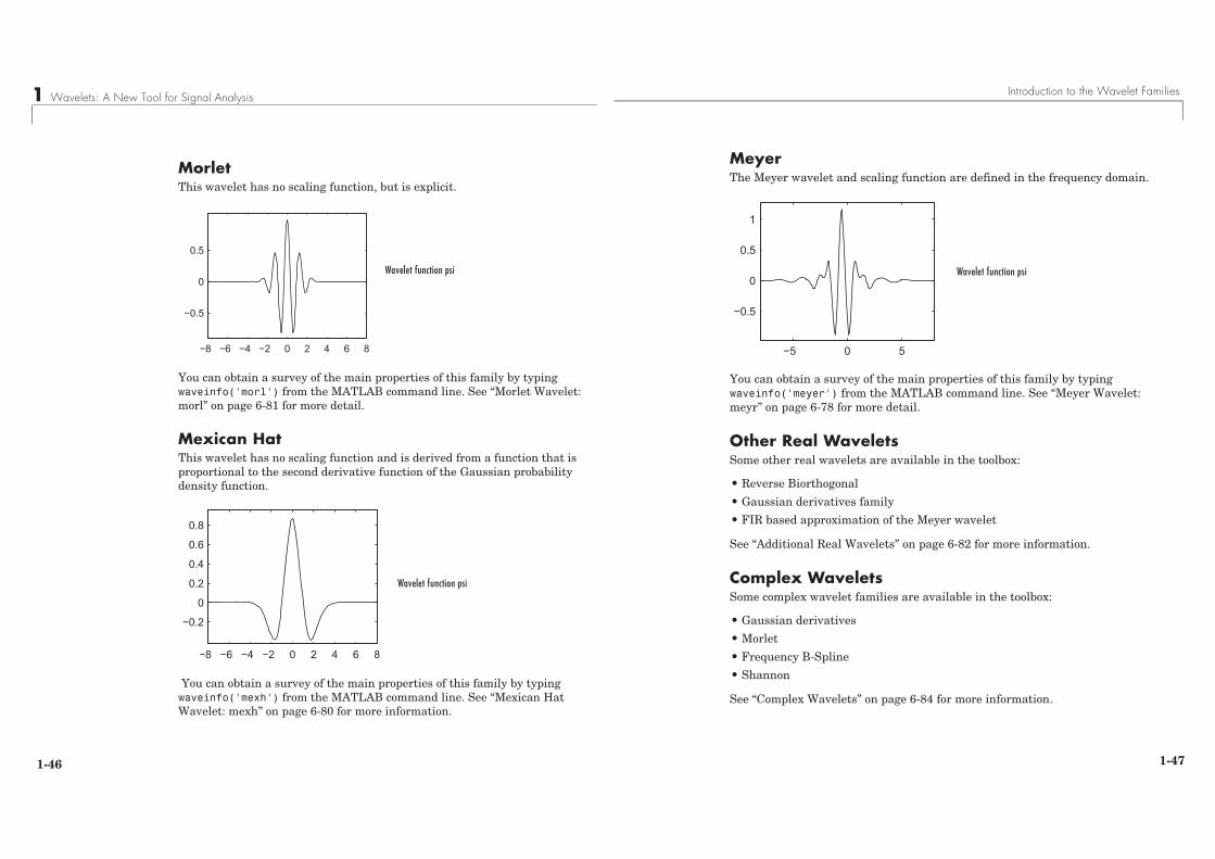
MorletThis wavelet has no scaling function, but is explicit.

You can obtain a survey of the main properties of this family by typing waveinfo('morl') from the MATLAB command line. See “Morlet Wavelet: morl” on page 6-81 for more detail.

Mexican HatThis wavelet has no scaling function and is derived from a function that is proportional to the second derivative function of the Gaussian probability density function.

You can obtain a survey of the main properties of this family by typing waveinfo('mexh') from the MATLAB command line. See “Mexican Hat Wavelet: mexh” on page 6-80 for more information.

−8 −6 −4 −2 0 2 4 6 8

−0.5

0

0.5


−8 −6 −4 −2 0 2 4 6 8

−0.2

0

0.2

0.4

0.6

0.8



1-47

MeyerThe Meyer wavelet and scaling function are defined in the frequency domain.

You can obtain a survey of the main properties of this family by typing waveinfo('meyer') from the MATLAB command line. See “Meyer Wavelet: meyr” on page 6-78 for more detail.

Other Real WaveletsSome other real wavelets are available in the toolbox:

• Reverse Biorthogonal

• Gaussian derivatives family

• FIR based approximation of the Meyer wavelet

See “Additional Real Wavelets” on page 6-82 for more information.

Complex WaveletsSome complex wavelet families are available in the toolbox:

• Gaussian derivatives

• Morlet

• Frequency B-Spline

• Shannon

See “Complex Wavelets” on page 6-84 for more information.

−5 0 5

−0.5

0

0.5

1


2 Using Wavelets

2-4

One-Dimensional Continuous Wavelet AnalysisThis section takes you through the features of continuous wavelet analysis using Wavelet Toolbox™ software.

The toolbox requires only one function for continuous wavelet analysis: cwt. You’ll find full information about this function in its reference page.

In this section, you’ll learn how to

• Load a signal

• Perform a continuous wavelet transform of a signal

• Produce a plot of the coefficients

• Produce a plot of coefficients at a given scale

• Produce a plot of local maxima of coefficients across scales

• Select the displayed plots

• Switch from scale to pseudo-frequency information

• Zoom in on detail

• Display coefficients in normal or absolute mode

• Choose the scales at which analysis is performed

Since you can perform analyses either from the command line or using the graphical interface tools, this section has subsections covering each method.

The final subsection discusses how to exchange signal and coefficient information between the disk and the graphical tools.

One-Dimensional Continuous Wavelet Analysis

2-5

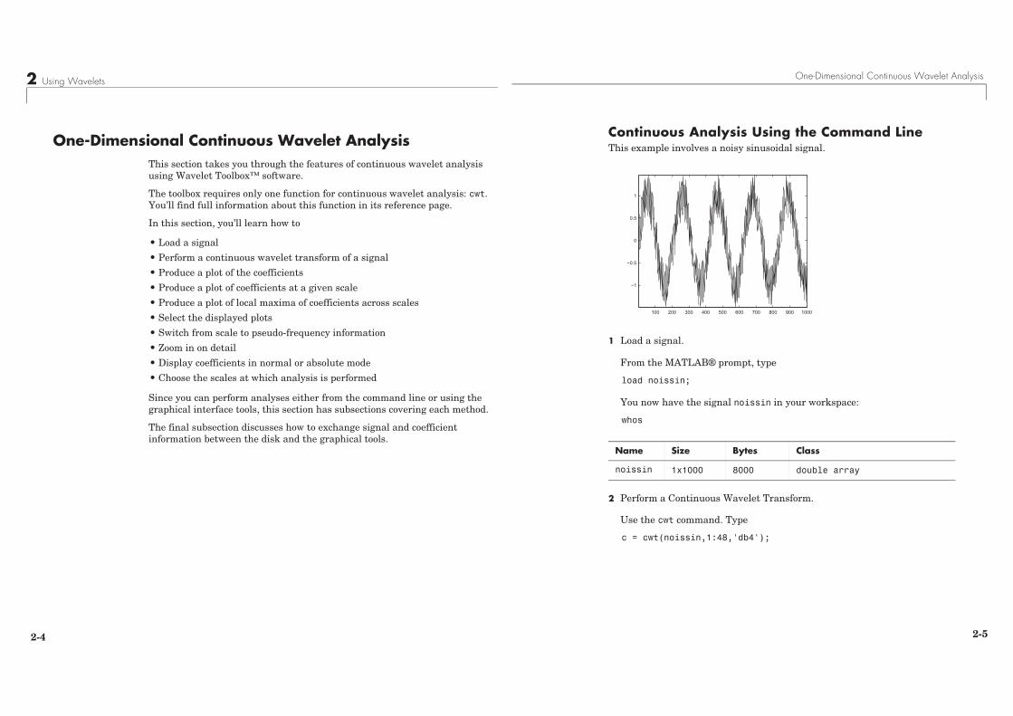
Continuous Analysis Using the Command LineThis example involves a noisy sinusoidal signal.

1 Load a signal.

From the MATLAB® prompt, type

load noissin;

You now have the signal noissin in your workspace:

whos

2 Perform a Continuous Wavelet Transform.

Use the cwt command. Type

c = cwt(noissin,1:48,'db4');

Name Size Bytes Class

noissin 1x1000 8000 double array

100 200 300 400 500 600 700 800 900 1000

−1

−0.5

0

0.5

1

2 Using Wavelets

2-6

The arguments to cwt specify the signal to be analyzed, the scales of the analysis, and the wavelet to be used. The returned argument c contains the coefficients at various scales. In this case, c is a 48-by-1000 matrix with each row corresponding to a single scale.

3 Plot the coefficients.

The cwt command accepts a fourth argument. This is a flag that, when present, causes cwt to produce a plot of the absolute values of the continuous wavelet transform coefficients.

The cwt command can accept more arguments to define the different characteristics of the produced plot. For more information, see the cwt reference page.

c = cwt(noissin,1:48,'db4','plot');

A plot appears.

Of course, coefficient plots generated from the command line can be manipulated using ordinary MATLAB graphics commands.

Absolute Values of Ca,b Coefficients for a = 1 2 3 4 5 ...

time (or space) b

scal

es a

100 200 300 400 500 600 700 800 900 1000 1

4

7

10

13

16

19

22

25

28

31

34

37

40

43

46


2-7

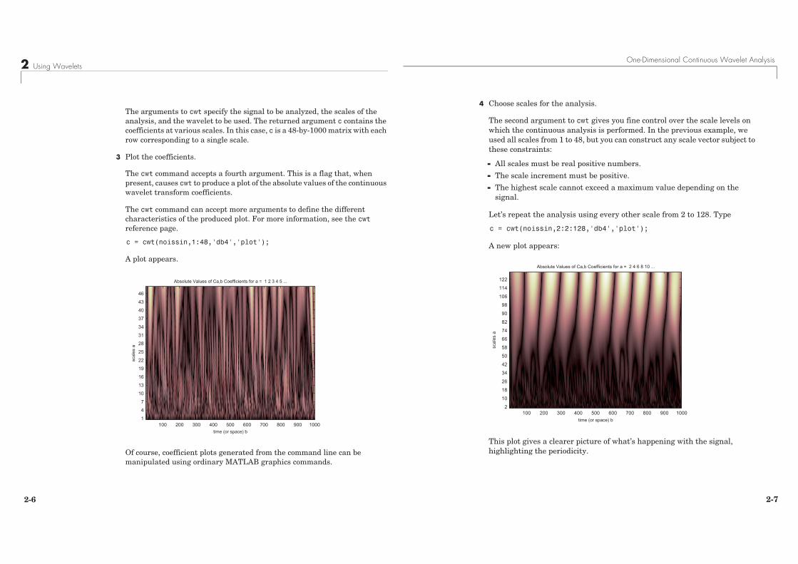
4 Choose scales for the analysis.

The second argument to cwt gives you fine control over the scale levels on which the continuous analysis is performed. In the previous example, we used all scales from 1 to 48, but you can construct any scale vector subject to these constraints:

- All scales must be real positive numbers.

- The scale increment must be positive.

- The highest scale cannot exceed a maximum value depending on the signal.

Let’s repeat the analysis using every other scale from 2 to 128. Type

c = cwt(noissin,2:2:128,'db4','plot');

A new plot appears:

This plot gives a clearer picture of what’s happening with the signal, highlighting the periodicity.

Absolute Values of Ca,b Coefficients for a = 2 4 6 8 10 ...

time (or space) b

scal

es a

100 200 300 400 500 600 700 800 900 1000 2

10

18

26

34

42

50

58

66

74

82

90

98

106

114

122

2 Using Wavelets

2-8

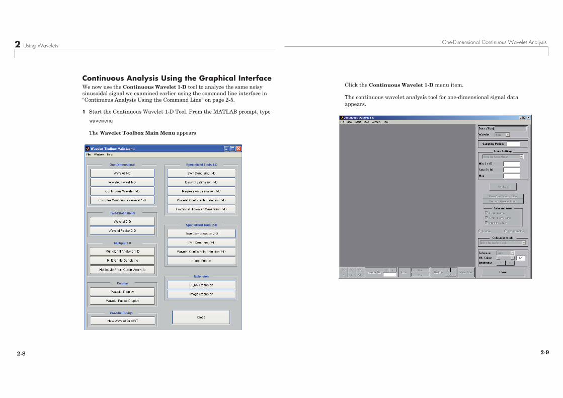
Continuous Analysis Using the Graphical InterfaceWe now use the Continuous Wavelet 1-D tool to analyze the same noisy sinusoidal signal we examined earlier using the command line interface in “Continuous Analysis Using the Command Line” on page 2-5.

1 Start the Continuous Wavelet 1-D Tool. From the MATLAB prompt, type

wavemenu

The Wavelet Toolbox Main Menu appears.


2-9

Click the Continuous Wavelet 1-D menu item.

The continuous wavelet analysis tool for one-dimensional signal data appears.

2 Using Wavelets

2-10

2 Load a signal.

Choose the File > Load Signal menu option.

When the Load Signal dialog box appears, select the demo MAT-file noissin.mat, which should reside in the MATLAB directory toolbox/wavelet/wavedemo. Click the OK button.

The noisy sinusoidal signal is loaded into the Continuous Wavelet 1-D tool.

The default value for the sampling period is equal to 1 (second).


To start our analysis, let’s perform an analysis using the db4 wavelet at scales 1 through 48, just as we did using command line functions in the previous section.

In the upper right portion of the Continuous Wavelet 1-D tool, select the db4 wavelet and scales 1–48.

Select db4

Select scales 1 to 48 in steps of 1


2-11

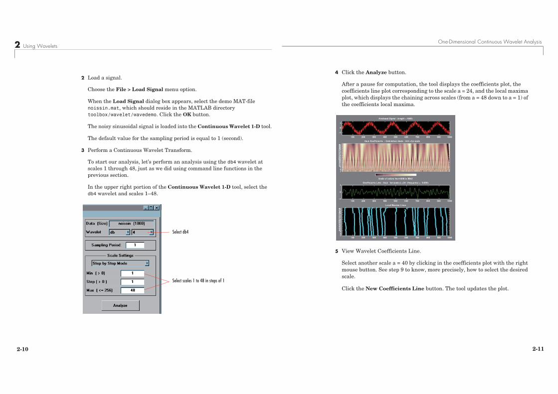
4 Click the Analyze button.

After a pause for computation, the tool displays the coefficients plot, the coefficients line plot corresponding to the scale a = 24, and the local maxima plot, which displays the chaining across scales (from a = 48 down to a = 1) of the coefficients local maxima.

.

5 View Wavelet Coefficients Line.

Select another scale a = 40 by clicking in the coefficients plot with the right mouse button. See step 9 to know, more precisely, how to select the desired scale.

Click the New Coefficients Line button. The tool updates the plot.

2 Using Wavelets

2-12

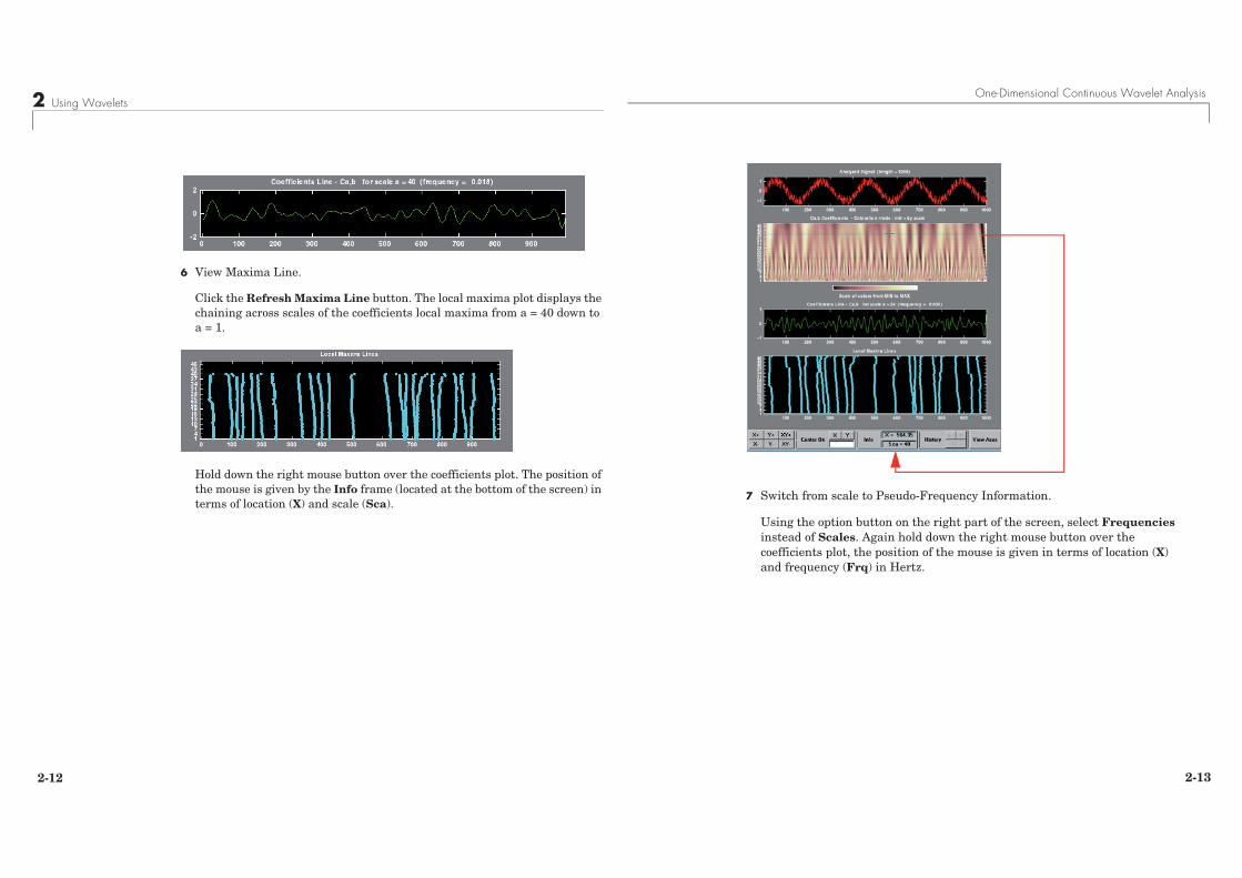
6 View Maxima Line.

Click the Refresh Maxima Line button. The local maxima plot displays the chaining across scales of the coefficients local maxima from a = 40 down to a = 1.

Hold down the right mouse button over the coefficients plot. The position of the mouse is given by the Info frame (located at the bottom of the screen) in terms of location (X) and scale (Sca).


2-13

7 Switch from scale to Pseudo-Frequency Information.

Using the option button on the right part of the screen, select Frequencies instead of Scales. Again hold down the right mouse button over the coefficients plot, the position of the mouse is given in terms of location (X) and frequency (Frq) in Hertz.

2 Using Wavelets

2-14

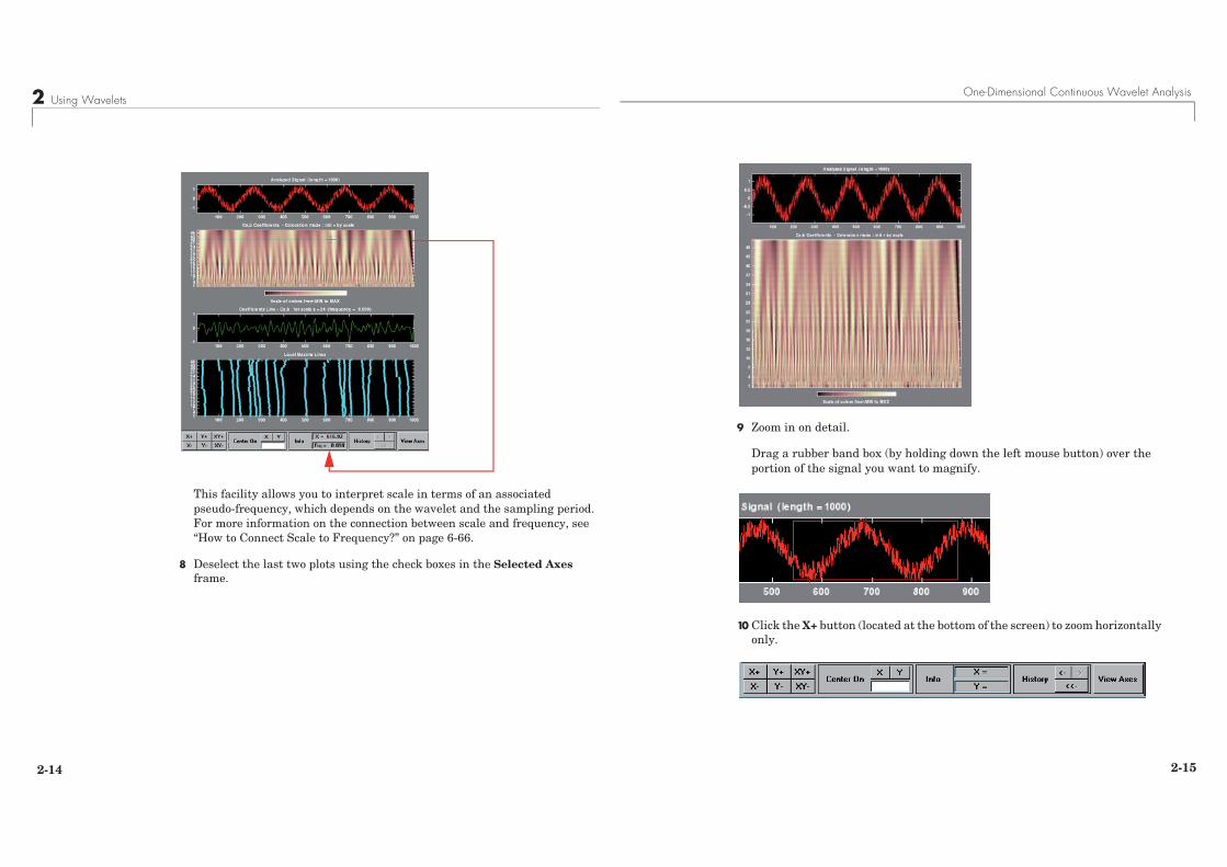
This facility allows you to interpret scale in terms of an associated pseudo-frequency, which depends on the wavelet and the sampling period. For more information on the connection between scale and frequency, see “How to Connect Scale to Frequency?” on page 6-66.

8 Deselect the last two plots using the check boxes in the Selected Axes frame.


2-15

.

9 Zoom in on detail.

Drag a rubber band box (by holding down the left mouse button) over the portion of the signal you want to magnify.

.

10 Click the X+ button (located at the bottom of the screen) to zoom horizontally only.

2 Using Wavelets

2-16

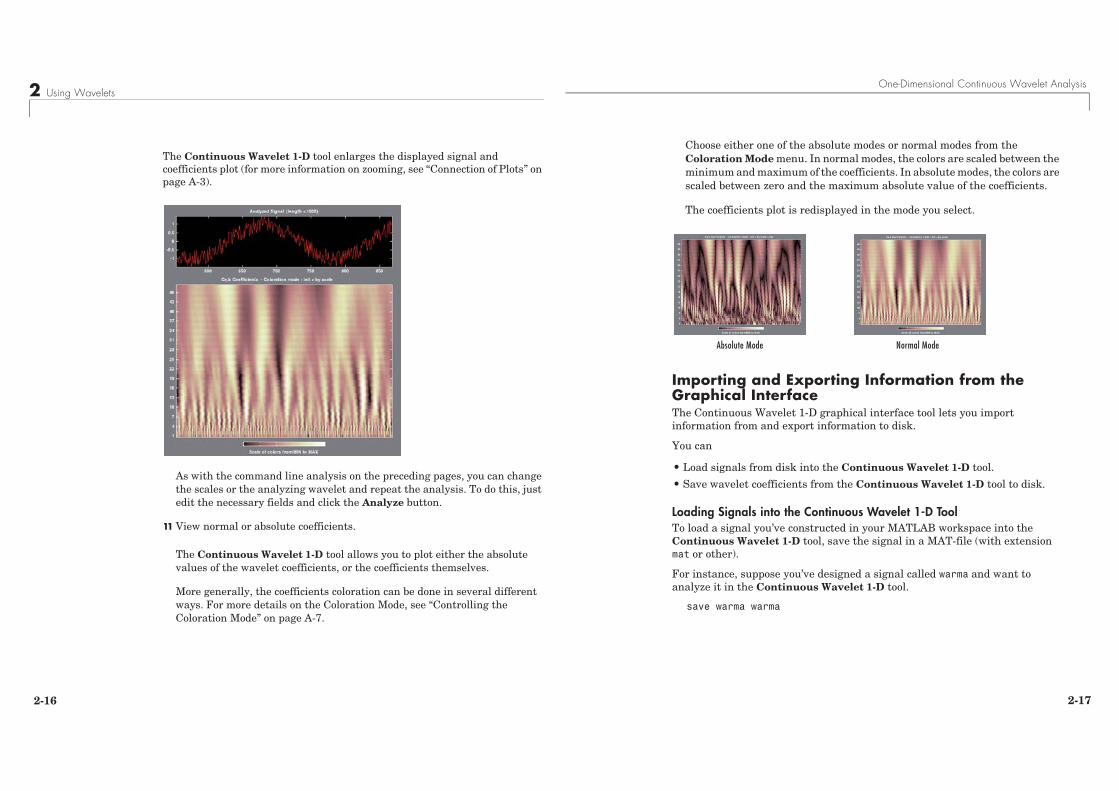
The Continuous Wavelet 1-D tool enlarges the displayed signal and coefficients plot (for more information on zooming, see “Connection of Plots” on page A-3).

As with the command line analysis on the preceding pages, you can change the scales or the analyzing wavelet and repeat the analysis. To do this, just edit the necessary fields and click the Analyze button.

11 View normal or absolute coefficients.

The Continuous Wavelet 1-D tool allows you to plot either the absolute values of the wavelet coefficients, or the coefficients themselves.

More generally, the coefficients coloration can be done in several different ways. For more details on the Coloration Mode, see “Controlling the Coloration Mode” on page A-7.


2-17

Choose either one of the absolute modes or normal modes from the Coloration Mode menu. In normal modes, the colors are scaled between the minimum and maximum of the coefficients. In absolute modes, the colors are scaled between zero and the maximum absolute value of the coefficients.

The coefficients plot is redisplayed in the mode you select.

Importing and Exporting Information from theGraphical InterfaceThe Continuous Wavelet 1-D graphical interface tool lets you import information from and export information to disk.

You can

• Load signals from disk into the Continuous Wavelet 1-D tool.

• Save wavelet coefficients from the Continuous Wavelet 1-D tool to disk.

Loading Signals into the Continuous Wavelet 1-D ToolTo load a signal you’ve constructed in your MATLAB workspace into the Continuous Wavelet 1-D tool, save the signal in a MAT-file (with extension mat or other).

For instance, suppose you’ve designed a signal called warma and want to analyze it in the Continuous Wavelet 1-D tool.

save warma warma

Absolute Mode Normal Mode

2 Using Wavelets

2-18

The workspace variable warma must be a vector.

sizwarma = size(warma)

sizwarma = 1 1000

To load this signal into the Continuous Wavelet 1-D tool, use the menu option File > Load Signal. A dialog box appears that lets you select the appropriate MAT-file to be loaded.

Note The first one-dimensional variable encountered in the file is considered the signal. Variables are inspected in alphabetical order.

Saving Wavelet CoefficientsThe Continuous Wavelet 1-D tool lets you save wavelet coefficients to disk. The toolbox creates a MAT-file in the current directory with the extension wc1 and a name you give it.

To save the continuous wavelet coefficients from the present analysis, use the menu option File > Save > Coefficients.

A dialog box appears that lets you specify a directory and filename for storing the coefficients.

Consider the example analysis:

File > Example Analysis > with haar at scales [1:1:64] −−> Cantor curve.


2-19

After saving the continuous wavelet coefficients to the file cantor.wc1, load the variables into your workspace:

load cantor.wc1 -matwhos

Variables coefs and scales contain the continuous wavelet coefficients and the associated scales. More precisely, in the above example, coefs is a 64-by-2188 matrix, one row for each scale; and scales is the 1-by-64 vector 1:64. Variable wname contains the wavelet name.


coeff 64x2188 1120256 double array

scales 1x64 512 double array

wname 1x4 8 char array

2 Using Wavelets

2-20

One-Dimensional Complex Continuous Wavelet AnalysisThis section takes you through the features of complex continuous wavelet analysis using the Wavelet Toolbox™ software and focuses on the differences between the real and complex continuous analysis.

You can refer to the section “One-Dimensional Continuous Wavelet Analysis” on page 2-4 if you want to learn how to

• Zoom in on detail

• Display coefficients in normal or absolute mode

• Choose the scales at which the analysis is performed

• Switch from scale to pseudo-frequency information

• Exchange signal and coefficient information between the disk and the graphical tools

Wavelet Toolbox software requires only one function for complex continuous wavelet analysis of a real valued signal: cwt. You’ll find full information about this function in its reference page.


• Load a signal

• Perform a complex continuous wavelet transform of a signal

• Produce plots of the coefficients


One-Dimensional Complex Continuous Wavelet Analysis

2-21

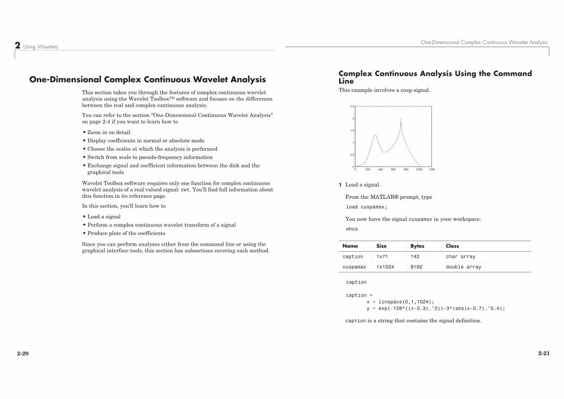
Complex Continuous Analysis Using the Command LineThis example involves a cusp signal.

1 Load a signal.


load cuspamax;

You now have the signal cuspamax in your workspace:

whos

caption

caption =x = linspace(0,1,1024);y = exp(-128*((x-0.3).^2))-3*(abs(x-0.7).^0.4);

caption is a string that contains the signal definition.


caption 1x71 142 char array

cuspamax 1x1024 8192 double array

0 200 400 600 800 1000 12000

0.5

1

1.5

2

2.5

2 Using Wavelets

2-22


Use the cwt command. Type

c = cwt(cuspamax,1:2:64,'cgau4');

The arguments to cwt specify the signal to be analyzed, the scales of the analysis, and the wavelet to be used. The returned argument c contains the coefficients at various scales. In this case, c is a complex 32-by-1024 matrix, each row of which corresponds to a single scale.

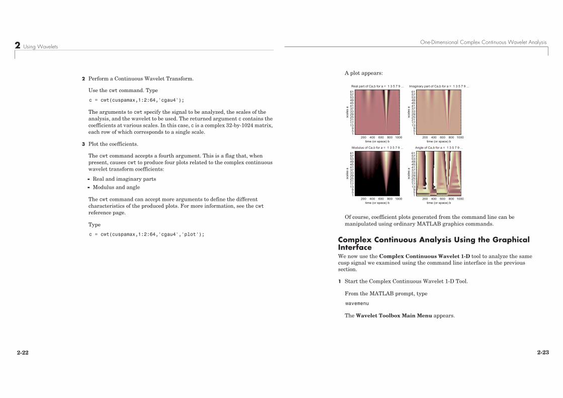
3 Plot the coefficients.

The cwt command accepts a fourth argument. This is a flag that, when present, causes cwt to produce four plots related to the complex continuous wavelet transform coefficients:

- Real and imaginary parts

- Modulus and angle

The cwt command can accept more arguments to define the different characteristics of the produced plots. For more information, see the cwt reference page.

Type

c = cwt(cuspamax,1:2:64,'cgau4','plot');


2-23

A plot appears:

Of course, coefficient plots generated from the command line can be manipulated using ordinary MATLAB graphics commands.

Complex Continuous Analysis Using the Graphical InterfaceWe now use the Complex Continuous Wavelet 1-D tool to analyze the same cusp signal we examined using the command line interface in the previous section.

1 Start the Complex Continuous Wavelet 1-D Tool.

From the MATLAB prompt, type

wavemenu


Real part of Ca,b for a = 1 3 5 7 9 ...

time (or space) b

scal

es a

200 400 600 800 1000 1 5 913172125293337414549535761

Imaginary part of Ca,b for a = 1 3 5 7 9 ...

time (or space) b

scal

es a

200 400 600 800 1000 1 5 913172125293337414549535761

Modulus of Ca,b for a = 1 3 5 7 9 ...

time (or space) b

scal

es a

200 400 600 800 1000 1 5 913172125293337414549535761

Angle of Ca,b for a = 1 3 5 7 9 ...

time (or space) b

scal

es a

200 400 600 800 1000 1 5 913172125293337414549535761

2 Using Wavelets

2-24

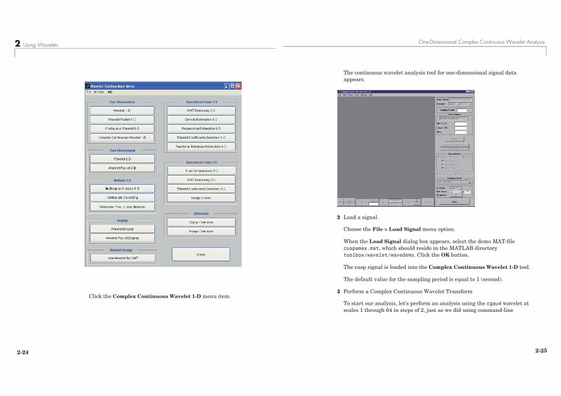
Click the Complex Continuous Wavelet 1-D menu item.


2-25

The continuous wavelet analysis tool for one-dimensional signal data appears.

2 Load a signal.

Choose the File > Load Signal menu option.

When the Load Signal dialog box appears, select the demo MAT-file cuspamax.mat, which should reside in the MATLAB directory toolbox/wavelet/wavedemo. Click the OK button.

The cusp signal is loaded into the Complex Continuous Wavelet 1-D tool.

The default value for the sampling period is equal to 1 (second).

3 Perform a Complex Continuous Wavelet Transform

To start our analysis, let’s perform an analysis using the cgau4 wavelet at scales 1 through 64 in steps of 2, just as we did using command-line

2 Using Wavelets

2-26

functions in “Complex Continuous Analysis Using the Command Line” on page 2-21.

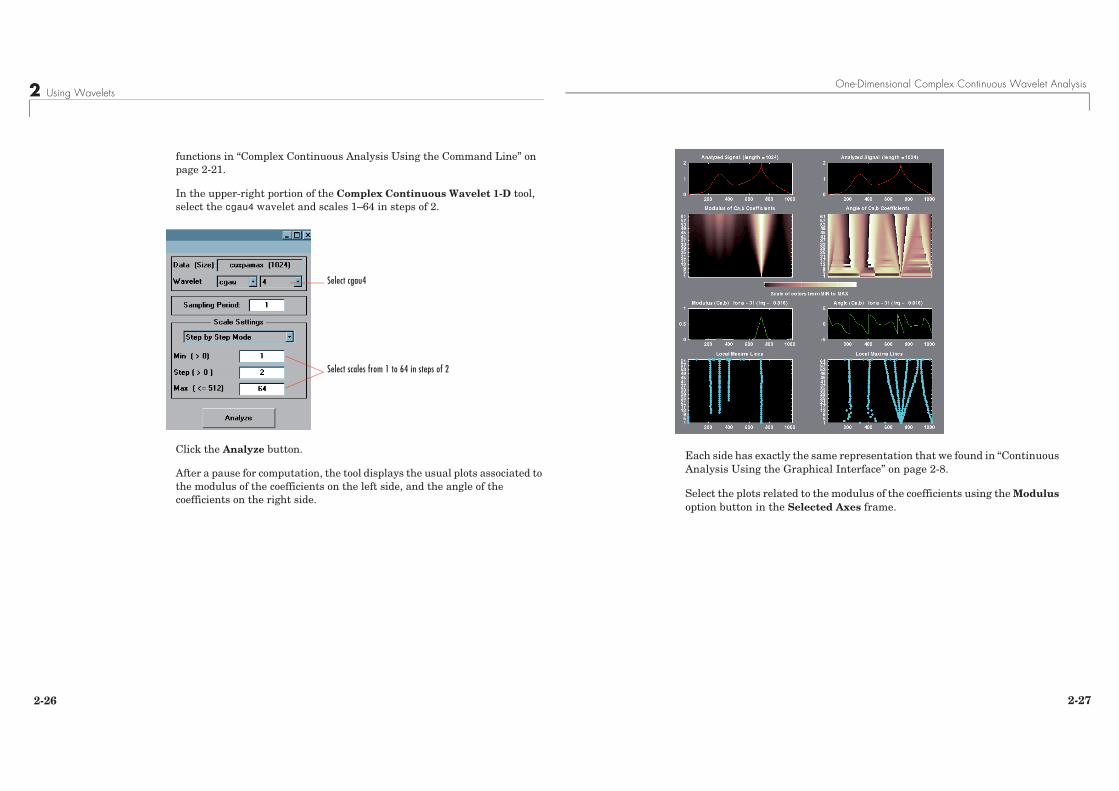
In the upper-right portion of the Complex Continuous Wavelet 1-D tool, select the cgau4 wavelet and scales 1–64 in steps of 2.

Click the Analyze button.

After a pause for computation, the tool displays the usual plots associated to the modulus of the coefficients on the left side, and the angle of the coefficients on the right side.

Select cgau4

Select scales from 1 to 64 in steps of 2


2-27

Each side has exactly the same representation that we found in “Continuous Analysis Using the Graphical Interface” on page 2-8.

Select the plots related to the modulus of the coefficients using the Modulus option button in the Selected Axes frame.

2 Using Wavelets

2-28

The figure now looks like the one in the real Continuous Wavelet 1-D tool.

Importing and Exporting Information from theGraphical InterfaceTo know how to import and export information from the Complex Continuous Wavelet Graphical Interface, see the corresponding paragraph in “One-Dimensional Continuous Wavelet Analysis” on page 2-4.

The only difference is that the variable coefs is a complex matrix (see “Saving Wavelet Coefficients” on page 2-18).

One-Dimensional Discrete Wavelet Analysis

2-29

One-Dimensional Discrete Wavelet AnalysisThis section takes you through the features of one-dimensional discrete wavelet analysis using the Wavelet Toolbox™ software.

The toolbox provides these functions for one-dimensional signal analysis. For more information, see the reference pages.

Analysis-Decomposition Functions

Synthesis-Reconstruction Functions

Decomposition Structure Utilities

Function Name Purpose

dwt Single-level decomposition

wavedec Decomposition

wmaxlev Maximum wavelet decomposition level


idwt Single-level reconstruction

waverec Full reconstruction

wrcoef Selective reconstruction

upcoef Single reconstruction


detcoef Extraction of detail coefficients

appcoef Extraction of approximation coefficients

upwlev Recomposition of decomposition structure

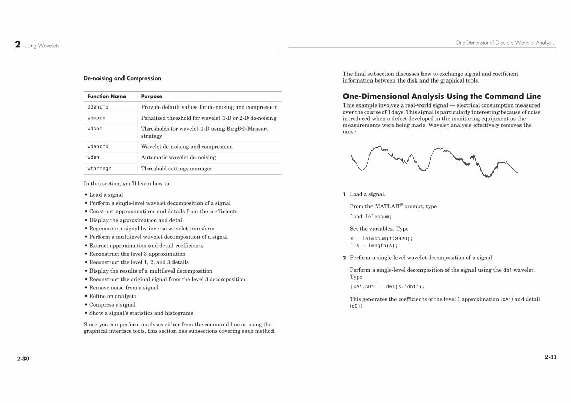
2 Using Wavelets

2-30

De-noising and Compression


• Load a signal

• Perform a single-level wavelet decomposition of a signal

• Construct approximations and details from the coefficients

• Display the approximation and detail

• Regenerate a signal by inverse wavelet transform

• Perform a multilevel wavelet decomposition of a signal

• Extract approximation and detail coefficients

• Reconstruct the level 3 approximation

• Reconstruct the level 1, 2, and 3 details

• Display the results of a multilevel decomposition

• Reconstruct the original signal from the level 3 decomposition

• Remove noise from a signal

• Refine an analysis

• Compress a signal

• Show a signal’s statistics and histograms



ddencmp Provide default values for de-noising and compression

wbmpen Penalized threshold for wavelet 1-D or 2-D de-noising

wdcbm Thresholds for wavelet 1-D using BirgÐ©-Massart strategy

wdencmp Wavelet de-noising and compression

wden Automatic wavelet de-noising

wthrmngr Threshold settings manager


2-31

The final subsection discusses how to exchange signal and coefficient information between the disk and the graphical tools.

One-Dimensional Analysis Using the Command LineThis example involves a real-world signal — electrical consumption measured over the course of 3 days. This signal is particularly interesting because of noise introduced when a defect developed in the monitoring equipment as the measurements were being made. Wavelet analysis effectively removes the noise.

1 Load a signal.


load leleccum;

Set the variables. Type

s = leleccum(1:3920); l_s = length(s);

2 Perform a single-level wavelet decomposition of a signal.

Perform a single-level decomposition of the signal using the db1 wavelet. Type

[cA1,cD1] = dwt(s,'db1');

This generates the coefficients of the level 1 approximation (cA1) and detail (cD1).

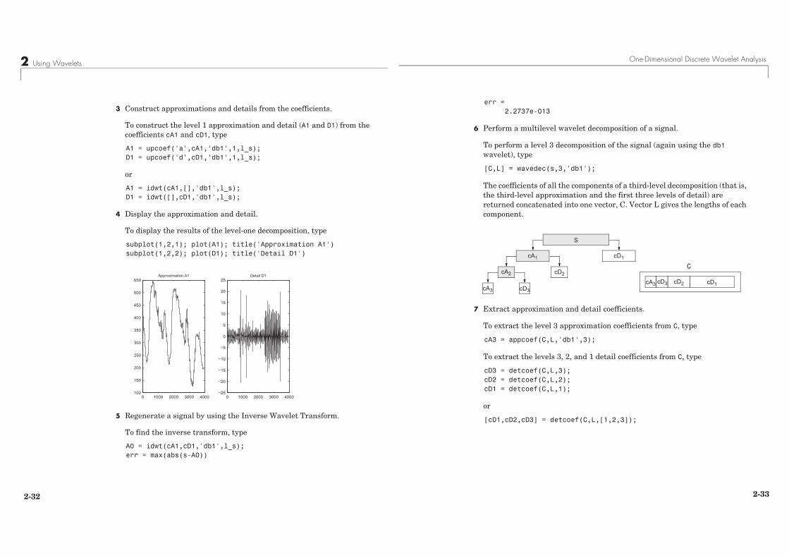
2 Using Wavelets

2-32

3 Construct approximations and details from the coefficients.

To construct the level 1 approximation and detail (A1 and D1) from the coefficients cA1 and cD1, type

A1 = upcoef('a',cA1,'db1',1,l_s); D1 = upcoef('d',cD1,'db1',1,l_s);

or

A1 = idwt(cA1,[],'db1',l_s); D1 = idwt([],cD1,'db1',l_s);

4 Display the approximation and detail.

To display the results of the level-one decomposition, type

subplot(1,2,1); plot(A1); title('Approximation A1')subplot(1,2,2); plot(D1); title('Detail D1')

5 Regenerate a signal by using the Inverse Wavelet Transform.

To find the inverse transform, type

A0 = idwt(cA1,cD1,'db1',l_s);err = max(abs(s-A0))

0 1000 2000 3000 4000100

150

200

250

300

350

400

450

500

550Approximation A1

0 1000 2000 3000 4000−25

−20

−15

−10

−5

0

5

10

15

20

25Detail D1


2-33

err = 2.2737e-013

6 Perform a multilevel wavelet decomposition of a signal.

To perform a level 3 decomposition of the signal (again using the db1 wavelet), type

[C,L] = wavedec(s,3,'db1');

The coefficients of all the components of a third-level decomposition (that is, the third-level approximation and the first three levels of detail) are returned concatenated into one vector, C. Vector L gives the lengths of each component.

7 Extract approximation and detail coefficients.

To extract the level 3 approximation coefficients from C, type

cA3 = appcoef(C,L,'db1',3);

To extract the levels 3, 2, and 1 detail coefficients from C, type

cD3 = detcoef(C,L,3); cD2 = detcoef(C,L,2); cD1 = detcoef(C,L,1);

or

[cD1,cD2,cD3] = detcoef(C,L,[1,2,3]);

S

cA1 cD1

cA2 cD2

cA3 cD3cD1cD2cA3 cD3

C

2 Using Wavelets

2-34

Results are displayed in the figure below, which contains the signal s, the approximation coefficients at level 3 (cA3), and the details coefficients from level 3 to 1 (cD3, cD2 and cD1) from the top to the bottom.

8 Reconstruct the Level 3 approximation and the Level 1, 2, and 3 details.

To reconstruct the level 3 approximation from C, type

A3 = wrcoef('a',C,L,'db1',3);

To reconstruct the details at levels 1, 2, and 3, from C, type

D1 = wrcoef('d',C,L,'db1',1);D2 = wrcoef('d',C,L,'db1',2);D3 = wrcoef('d',C,L,'db1',3);

0 5000

1000

20000 500 1000 1500 2000 2500 3000 3500 4000

0

500

1000Original signal s and coefficients.

0 500−100

0

100

0 500 1000−50

0

50

0 500 1000 1500 2000−50

0

50


2-35

9 Display the results of a multilevel decomposition.

To display the results of the level 3 decomposition, type

subplot(2,2,1); plot(A3); title('Approximation A3')subplot(2,2,2); plot(D1); title('Detail D1')subplot(2,2,3); plot(D2); title('Detail D2')subplot(2,2,4); plot(D3); title('Detail D3')

10 Reconstruct the original signal from the Level 3 decomposition.

To reconstruct the original signal from the wavelet decomposition structure, type

A0 = waverec(C,L,'db1');

err = max(abs(s-A0))

err = 4.5475e-013

0 1000 2000 3000 4000100

200

300

400

500

600Approximation A3

0 1000 2000 3000 4000−40

−20

0

20

40Detail D1

0 1000 2000 3000 4000−40

−20

0

20

40Detail D2

0 1000 2000 3000 4000−40

−20

0

20

40Detail D3

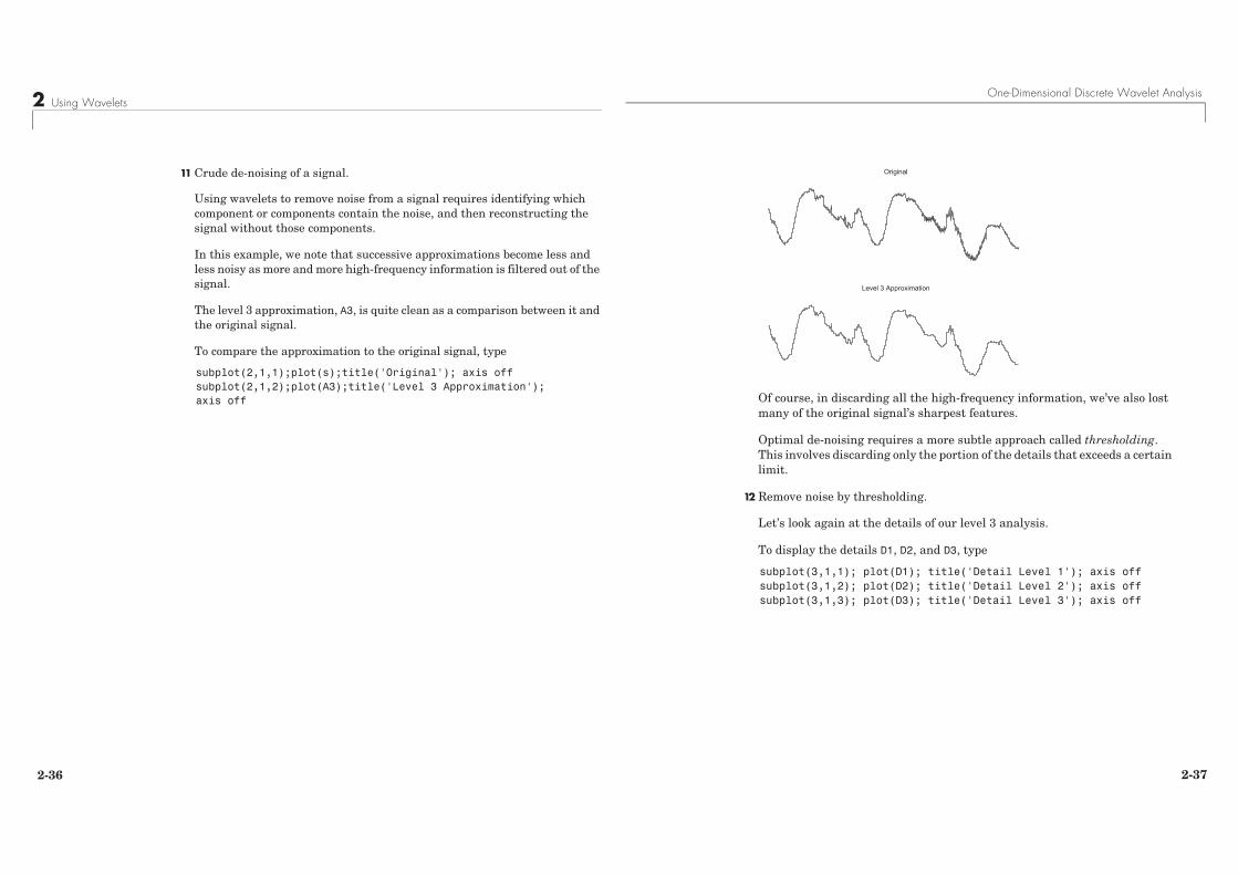
2 Using Wavelets

2-36

11 Crude de-noising of a signal.

Using wavelets to remove noise from a signal requires identifying which component or components contain the noise, and then reconstructing the signal without those components.

In this example, we note that successive approximations become less and less noisy as more and more high-frequency information is filtered out of the signal.

The level 3 approximation, A3, is quite clean as a comparison between it and the original signal.

To compare the approximation to the original signal, type

subplot(2,1,1);plot(s);title('Original'); axis offsubplot(2,1,2);plot(A3);title('Level 3 Approximation');axis off


2-37

Of course, in discarding all the high-frequency information, we’ve also lost many of the original signal’s sharpest features.

Optimal de-noising requires a more subtle approach called thresholding. This involves discarding only the portion of the details that exceeds a certain limit.

12 Remove noise by thresholding.

Let’s look again at the details of our level 3 analysis.

To display the details D1, D2, and D3, type

subplot(3,1,1); plot(D1); title('Detail Level 1'); axis offsubplot(3,1,2); plot(D2); title('Detail Level 2'); axis offsubplot(3,1,3); plot(D3); title('Detail Level 3'); axis off

Original

Level 3 Approximation

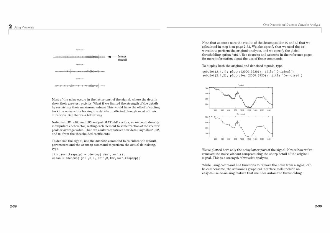
2 Using Wavelets

2-38

Most of the noise occurs in the latter part of the signal, where the details show their greatest activity. What if we limited the strength of the details by restricting their maximum values? This would have the effect of cutting back the noise while leaving the details unaffected through most of their durations. But there’s a better way.

Note that cD1, cD2, and cD3 are just MATLAB vectors, so we could directly manipulate each vector, setting each element to some fraction of the vectors’ peak or average value. Then we could reconstruct new detail signals D1, D2, and D3 from the thresholded coefficients.

To denoise the signal, use the ddencmp command to calculate the default parameters and the wdencmp command to perform the actual de-noising, type

[thr,sorh,keepapp] = ddencmp('den','wv',s);clean = wdencmp('gbl',C,L,'db1',3,thr,sorh,keepapp);

Detail Level 1

Detail Level 2

Detail Level 3

Setting a threshold


2-39

Note that wdencmp uses the results of the decomposition (C and L) that we calculated in step 6 on page 2-33. We also specify that we used the db1 wavelet to perform the original analysis, and we specify the global thresholding option 'gbl'. See ddencmp and wdencmp in the reference pages for more information about the use of these commands.

To display both the original and denoised signals, type

subplot(2,1,1); plot(s(2000:3920)); title('Original')subplot(2,1,2); plot(clean(2000:3920)); title('De-noised')

We’ve plotted here only the noisy latter part of the signal. Notice how we’ve removed the noise without compromising the sharp detail of the original signal. This is a strength of wavelet analysis.

While using command line functions to remove the noise from a signal can be cumbersome, the software’s graphical interface tools include an easy-to-use de-noising feature that includes automatic thresholding.

200 400 600 800 1000 1200 1400 1600 1800

200

300

400

500

Original

200 400 600 800 1000 1200 1400 1600 1800

200

300

400

500De−noised

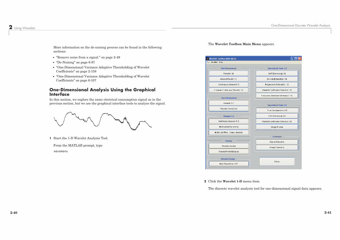
2 Using Wavelets

2-40

More information on the de-noising process can be found in the following sections:

- “Remove noise from a signal.” on page 2-49

- “De-Noising” on page 6-97

- “One-Dimensional Variance Adaptive Thresholding of Wavelet Coefficients” on page 2-158

- “One-Dimensional Variance Adaptive Thresholding of Wavelet Coefficients” on page 6-107

One-Dimensional Analysis Using the Graphical InterfaceIn this section, we explore the same electrical consumption signal as in the previous section, but we use the graphical interface tools to analyze the signal.

1 Start the 1-D Wavelet Analysis Tool.

From the MATLAB prompt, type

wavemenu


2-41


2 Click the Wavelet 1-D menu item.

The discrete wavelet analysis tool for one-dimensional signal data appears.

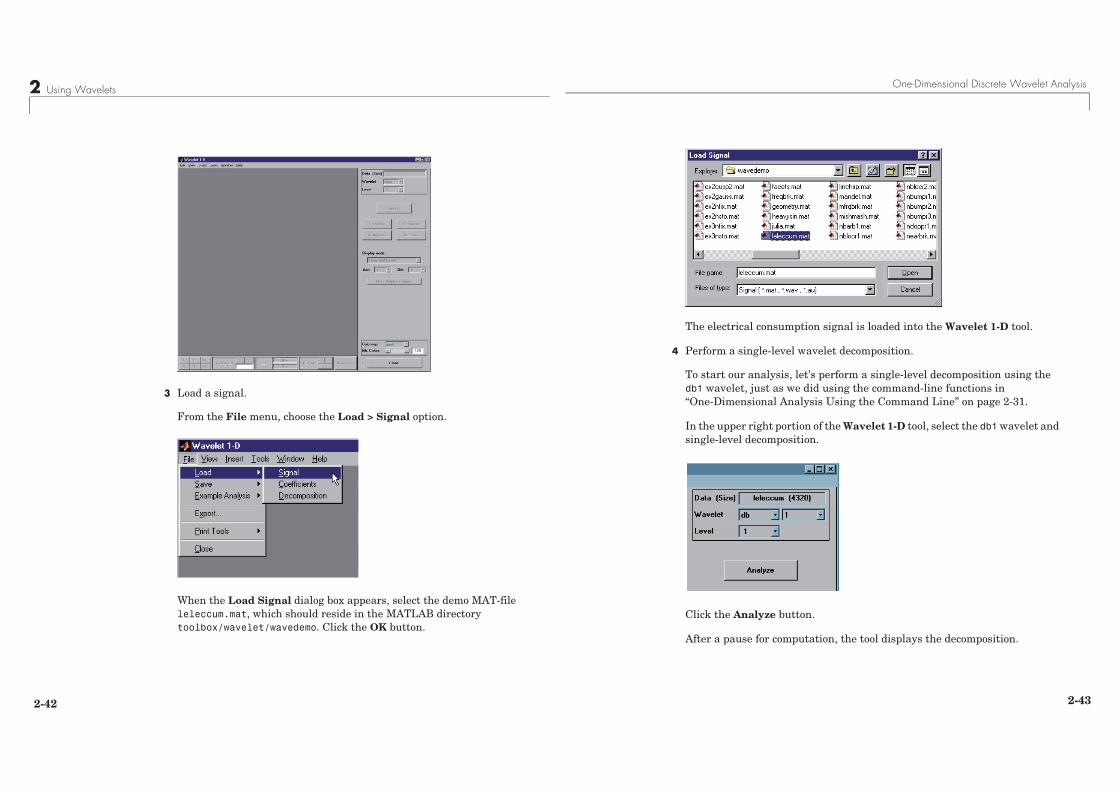
2 Using Wavelets

2-42

3 Load a signal.

From the File menu, choose the Load > Signal option.

When the Load Signal dialog box appears, select the demo MAT-file leleccum.mat, which should reside in the MATLAB directory toolbox/wavelet/wavedemo. Click the OK button.


2-43

The electrical consumption signal is loaded into the Wavelet 1-D tool.

4 Perform a single-level wavelet decomposition.

To start our analysis, let’s perform a single-level decomposition using the db1 wavelet, just as we did using the command-line functions in “One-Dimensional Analysis Using the Command Line” on page 2-31.

In the upper right portion of the Wavelet 1-D tool, select the db1 wavelet and single-level decomposition.

Click the Analyze button.

After a pause for computation, the tool displays the decomposition.

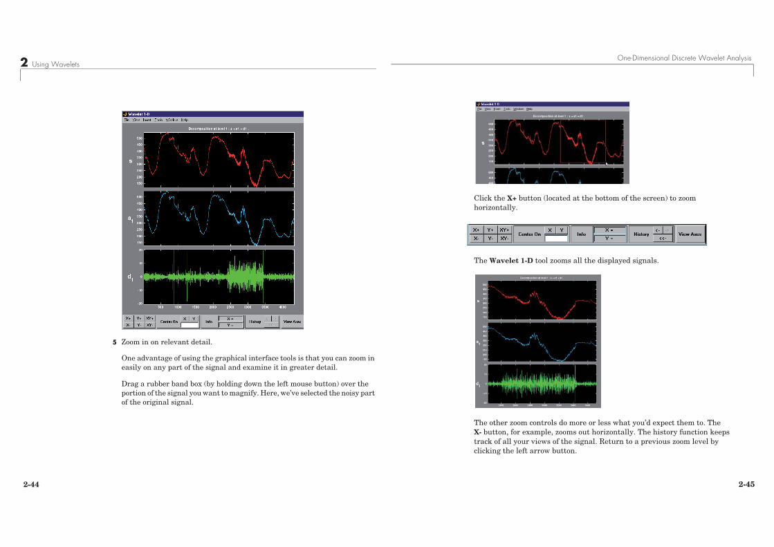
2 Using Wavelets

2-44

5 Zoom in on relevant detail.

One advantage of using the graphical interface tools is that you can zoom in easily on any part of the signal and examine it in greater detail.

Drag a rubber band box (by holding down the left mouse button) over the portion of the signal you want to magnify. Here, we’ve selected the noisy part of the original signal.


2-45

Click the X+ button (located at the bottom of the screen) to zoom horizontally.

The Wavelet 1-D tool zooms all the displayed signals.

The other zoom controls do more or less what you’d expect them to. The X- button, for example, zooms out horizontally. The history function keeps track of all your views of the signal. Return to a previous zoom level by clicking the left arrow button.

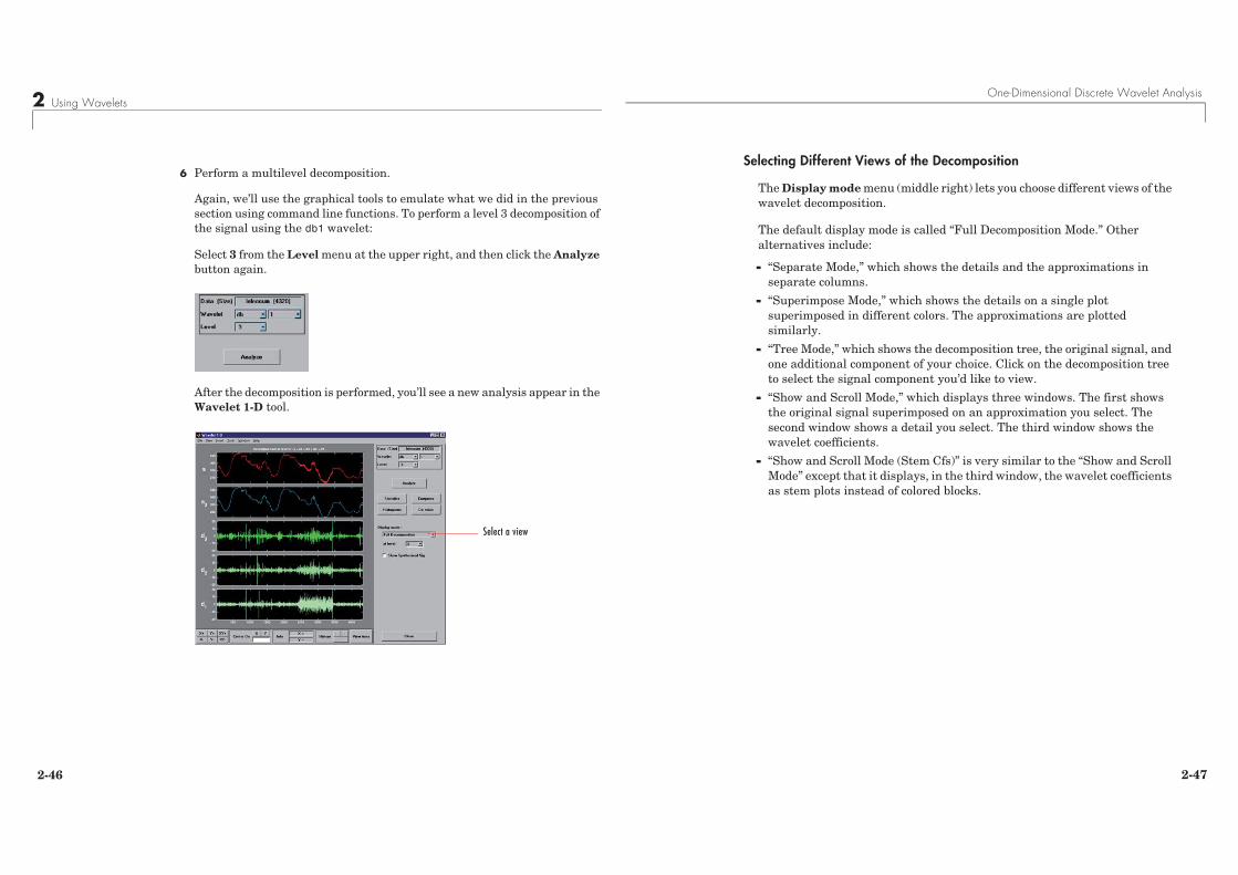
2 Using Wavelets

2-46

6 Perform a multilevel decomposition.

Again, we’ll use the graphical tools to emulate what we did in the previous section using command line functions. To perform a level 3 decomposition of the signal using the db1 wavelet:

Select 3 from the Level menu at the upper right, and then click the Analyze button again.

After the decomposition is performed, you’ll see a new analysis appear in the Wavelet 1-D tool.

Select a view


2-47

Selecting Different Views of the Decomposition

The Display mode menu (middle right) lets you choose different views of the wavelet decomposition.

The default display mode is called “Full Decomposition Mode.” Other alternatives include:

- “Separate Mode,” which shows the details and the approximations in separate columns.

- “Superimpose Mode,” which shows the details on a single plot superimposed in different colors. The approximations are plotted similarly.

- “Tree Mode,” which shows the decomposition tree, the original signal, and one additional component of your choice. Click on the decomposition tree to select the signal component you’d like to view.

- “Show and Scroll Mode,” which displays three windows. The first shows the original signal superimposed on an approximation you select. The second window shows a detail you select. The third window shows the wavelet coefficients.

- “Show and Scroll Mode (Stem Cfs)” is very similar to the “Show and Scroll Mode” except that it displays, in the third window, the wavelet coefficients as stem plots instead of colored blocks.

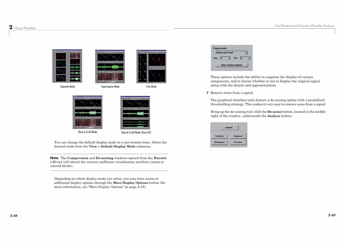
2 Using Wavelets

2-48

You can change the default display mode on a per-session basis. Select the desired mode from the View > Default Display Mode submenu.

Note The Compression and De-noising windows opened from the Wavelet 1-D tool will inherit the current coefficient visualization attribute (stems or colored blocks).

Depending on which display mode you select, you may have access to additional display options through the More Display Options button (for more information, see “More Display Options” on page A-19).

Separate Mode Superimpose Mode Tree Mode

Show & Scroll Mode Show & Scroll Mode (Stem Cfs)


2-49

These options include the ability to suppress the display of various components, and to choose whether or not to display the original signal along with the details and approximations.

7 Remove noise from a signal.

The graphical interface tools feature a de-noising option with a predefined thresholding strategy. This makes it very easy to remove noise from a signal.

Bring up the de-noising tool: click the De-noise button, located in the middle right of the window, underneath the Analyze button.

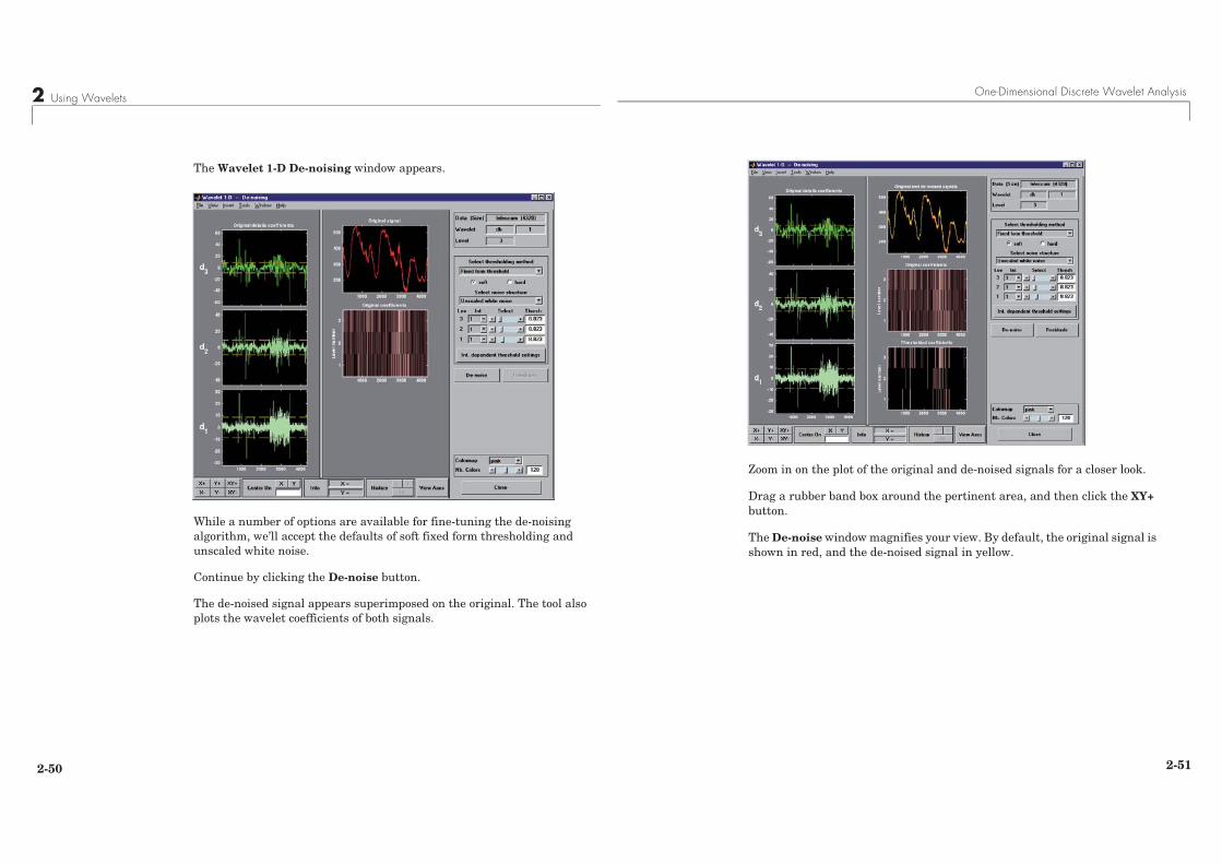
2 Using Wavelets

2-50

The Wavelet 1-D De-noising window appears.

While a number of options are available for fine-tuning the de-noising algorithm, we’ll accept the defaults of soft fixed form thresholding and unscaled white noise.

Continue by clicking the De-noise button.

The de-noised signal appears superimposed on the original. The tool also plots the wavelet coefficients of both signals.


2-51

Zoom in on the plot of the original and de-noised signals for a closer look.

Drag a rubber band box around the pertinent area, and then click the XY+ button.

The De-noise window magnifies your view. By default, the original signal is shown in red, and the de-noised signal in yellow.

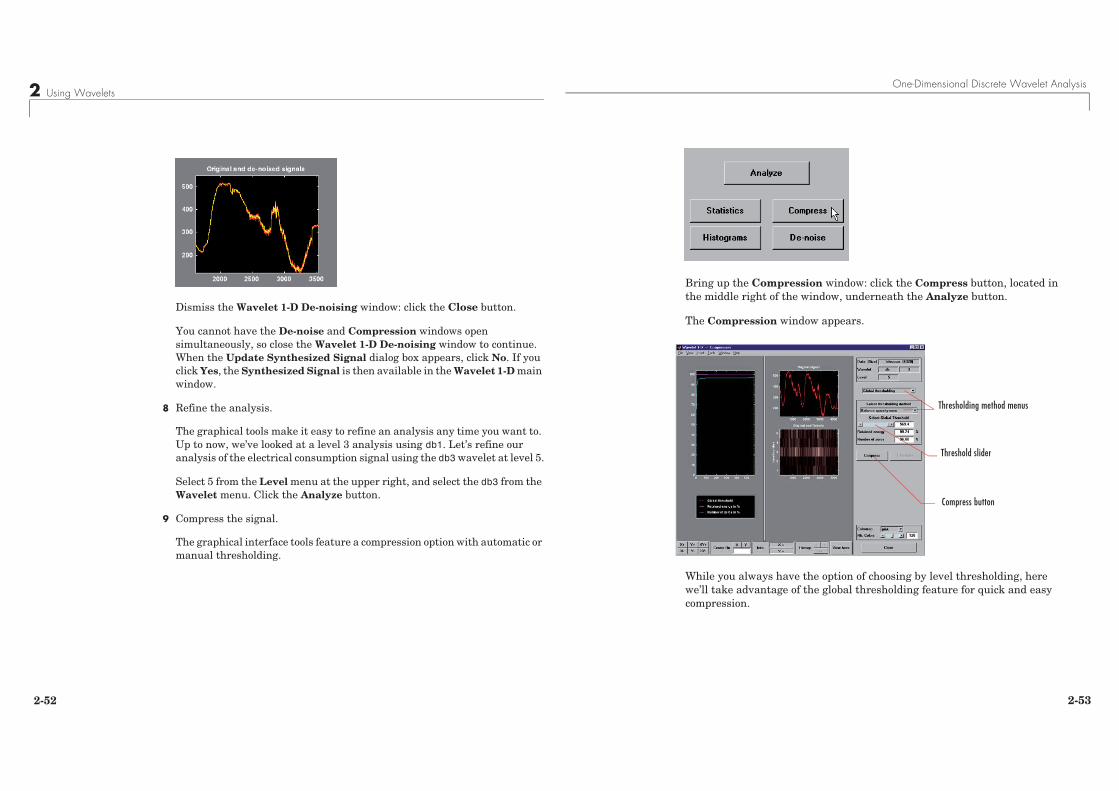
2 Using Wavelets

2-52

Dismiss the Wavelet 1-D De-noising window: click the Close button.

You cannot have the De-noise and Compression windows open simultaneously, so close the Wavelet 1-D De-noising window to continue. When the Update Synthesized Signal dialog box appears, click No. If you click Yes, the Synthesized Signal is then available in the Wavelet 1-D main window.

8 Refine the analysis.

The graphical tools make it easy to refine an analysis any time you want to. Up to now, we’ve looked at a level 3 analysis using db1. Let’s refine our analysis of the electrical consumption signal using the db3 wavelet at level 5.

Select 5 from the Level menu at the upper right, and select the db3 from the Wavelet menu. Click the Analyze button.

9 Compress the signal.

The graphical interface tools feature a compression option with automatic or manual thresholding.


2-53

Bring up the Compression window: click the Compress button, located in the middle right of the window, underneath the Analyze button.

The Compression window appears.

While you always have the option of choosing by level thresholding, here we’ll take advantage of the global thresholding feature for quick and easy compression.

Thresholding method menus

Threshold slider

Compress button

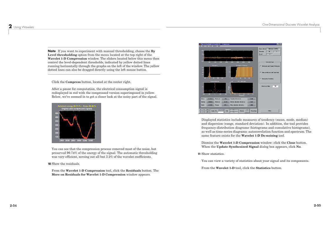
2 Using Wavelets

2-54

Note If you want to experiment with manual thresholding, choose the By Level thresholding option from the menu located at the top right of the Wavelet 1-D Compression window. The sliders located below this menu then control the level-dependent thresholds, indicated by yellow dotted lines running horizontally through the graphs on the left of the window. The yellow dotted lines can also be dragged directly using the left mouse button.

Click the Compress button, located at the center right.

After a pause for computation, the electrical consumption signal is redisplayed in red with the compressed version superimposed in yellow. Below, we’ve zoomed in to get a closer look at the noisy part of the signal.

You can see that the compression process removed most of the noise, but preserved 99.74% of the energy of the signal. The automatic thresholding was very efficient, zeroing out all but 3.2% of the wavelet coefficients.

10 Show the residuals.

From the Wavelet 1-D Compression tool, click the Residuals button. The More on Residuals for Wavelet 1-D Compression window appears.


2-55

Displayed statistics include measures of tendency (mean, mode, median) and dispersion (range, standard deviation). In addition, the tool provides frequency-distribution diagrams (histograms and cumulative histograms), as well as time-series diagrams: autocorrelation function and spectrum. The same feature exists for the Wavelet 1-D De-noising tool.

Dismiss the Wavelet 1-D Compression window: click the Close button. When the Update Synthesized Signal dialog box appears, click No.

11 Show statistics.

You can view a variety of statistics about your signal and its components.

From the Wavelet 1-D tool, click the Statistics button.

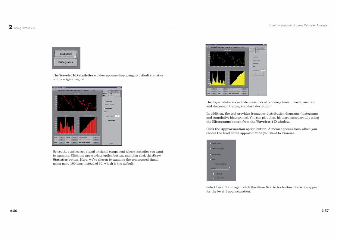
2 Using Wavelets

2-56

The Wavelet 1-D Statistics window appears displaying by default statistics on the original signal.

Select the synthesized signal or signal component whose statistics you want to examine. Click the appropriate option button, and then click the Show Statistics button. Here, we’ve chosen to examine the compressed signal using more 100 bins instead of 30, which is the default:


2-57

Displayed statistics include measures of tendency (mean, mode, median) and dispersion (range, standard deviation).

In addition, the tool provides frequency-distribution diagrams (histograms and cumulative histograms). You can plot these histograms separately using the Histograms button from the Wavelets 1-D window.

Click the Approximation option button. A menu appears from which you choose the level of the approximation you want to examine.

Select Level 1 and again click the Show Statistics button. Statistics appear for the level 1 approximation.

wavelet toolbox™ 4 - luleå university of technology/wavelet toolbox 4 user's guide... ·...

Documents