watershed delineation using arcmap
TRANSCRIPT
What is This?
Watershed Delineation by Arthur Gill Green is licensed under a Creative Commons Attribution-ShareAlike 4.0 International License.
Based on a work at http://greengeographer.com/.
• An open training module for learning Geographic Information Science as applied to watershed delineation. • It was developed for students at UBC. • It uses data from the USGS (SRTM) and
software from ESRI (ArcMap 10.3).
Why Do This Training?It’s free and you will learn how to:
• Get SRTM 1 Arc-Second (30 meter resolution) for free to make Digital Elevation Models (DEM).• Merge raster grids into mosaics. • Derive streams, stream orders, basins, and
specific watersheds from the data. • Convert raster grids into vector features. • Calculate area and length. • Create and analyze evidence for responding to
geographic questions.

Research QuestionWhile working in Cameroon on a transboundary international conservation area near Tchabal Mbabo, we wondered…
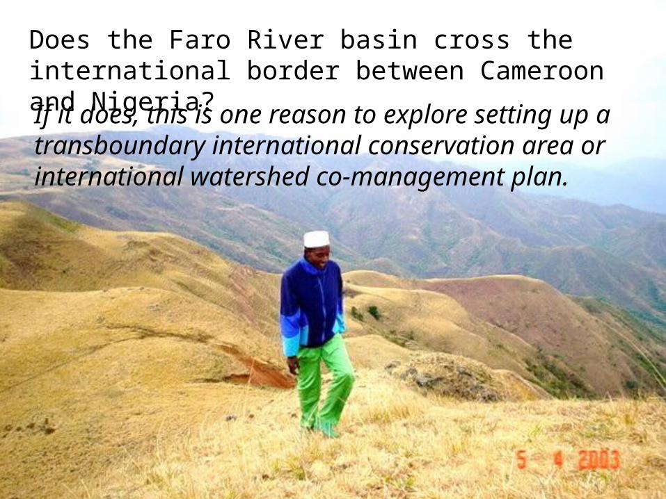
Does the Faro River basin cross the international border between Cameroon and Nigeria? If it does, this is one reason to explore setting up a transboundary international conservation area or international watershed co-management plan.
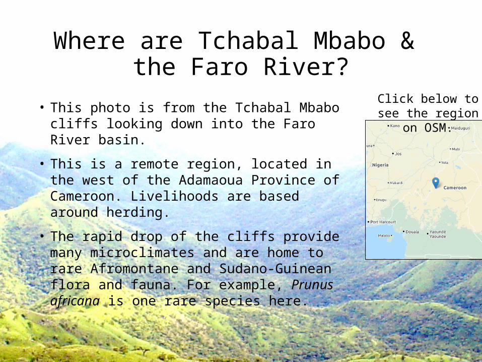
Where are Tchabal Mbabo & the Faro River?
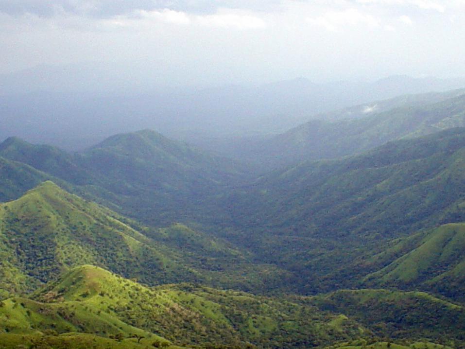
• This photo is from the Tchabal Mbabo cliffs looking down into the Faro River basin.
• This is a remote region, located in the west of the Adamaoua Province of Cameroon. Livelihoods are based around herding.
• The rapid drop of the cliffs provide many microclimates and are home to rare Afromontane and Sudano-Guinean flora and fauna. For example, Prunus africana is one rare species here.
Click below to see the region on
OSM.
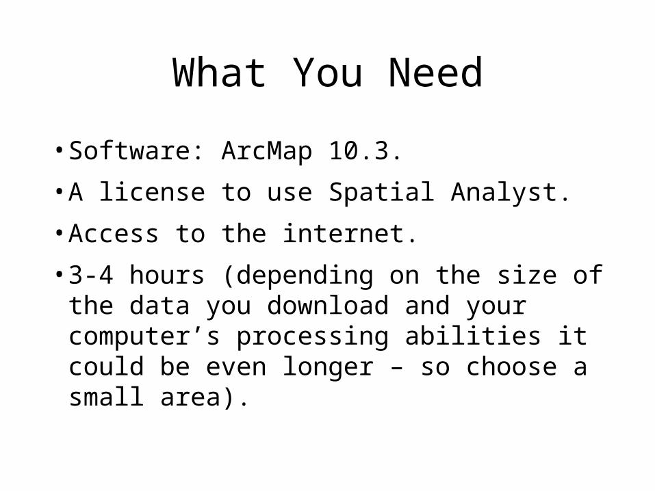
What You Need• Software: ArcMap 10.3.• A license to use Spatial Analyst. • Access to the internet.• 3-4 hours (depending on the size of the
data you download and your computer’s processing abilities it could be even longer – so choose a small area).
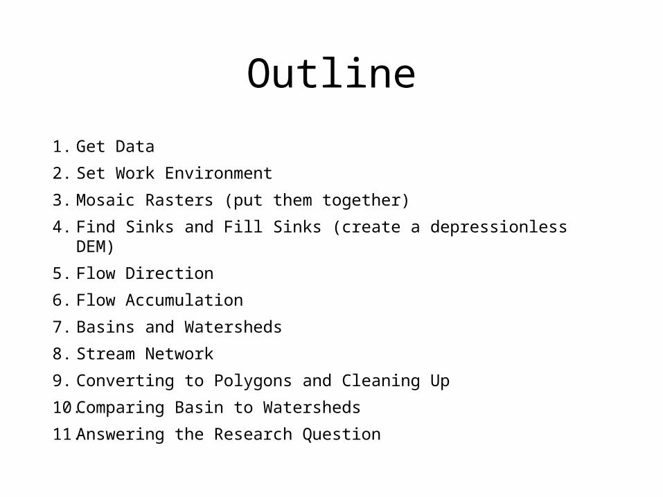
Outline1. Get Data2. Set Work Environment3. Mosaic Rasters (put them together)4. Find Sinks and Fill Sinks (create a depressionless DEM)5. Flow Direction6. Flow Accumulation7. Basins and Watersheds8. Stream Network9. Converting to Polygons and Cleaning Up10. Comparing Basin to Watersheds11. Answering the Research Question
1. Get Data
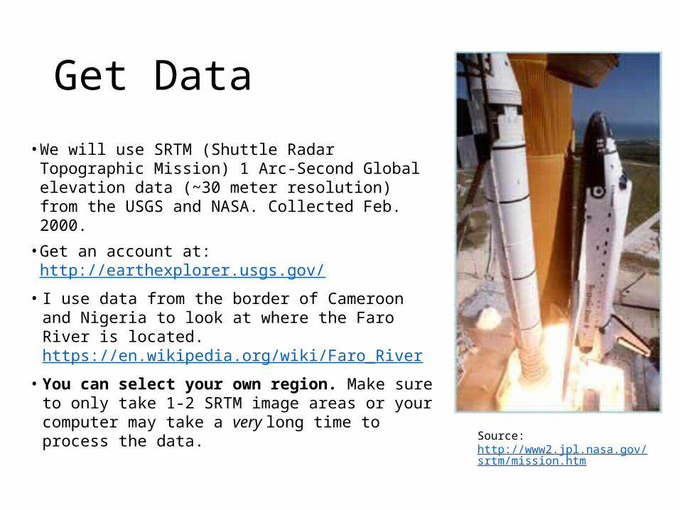
Get Data• We will use SRTM (Shuttle Radar
Topographic Mission) 1 Arc-Second Global elevation data (~30 meter resolution) from the USGS and NASA. Collected Feb. 2000.
• Get an account at: http://earthexplorer.usgs.gov/
• I use data from the border of Cameroon and Nigeria to look at where the Faro River is located. https://en.wikipedia.org/wiki/Faro_River
• You can select your own region. Make sure to only take 1-2 SRTM image areas or your computer may take a very long time to process the data. Source:
http://www2.jpl.nasa.gov/srtm/mission.htm
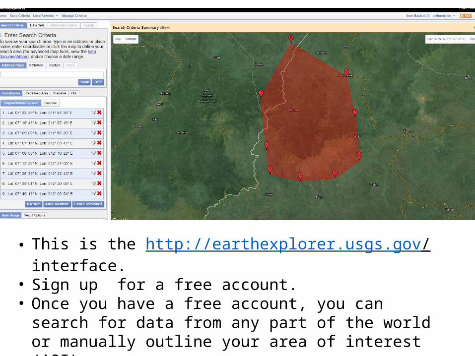
• This is the http://earthexplorer.usgs.gov/ interface.• Sign up for a free account.• Once you have a free account, you can search for
data from any part of the world or manually outline your area of interest (AOI).
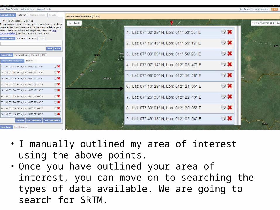
• I manually outlined my area of interest using the above points.
• Once you have outlined your area of interest, you can move on to searching the types of data available. We are going to search for SRTM.
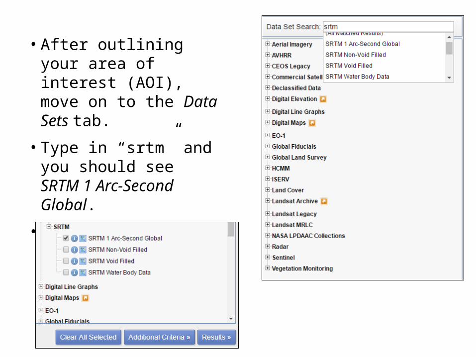
• After outlining your area of interest (AOI), move on to the Data Sets tab.• Type in “srtm” and
you should see SRTM 1 Arc-Second Global.• Select that, then click
on Results.
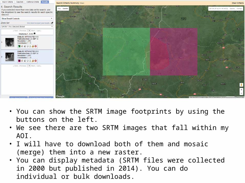
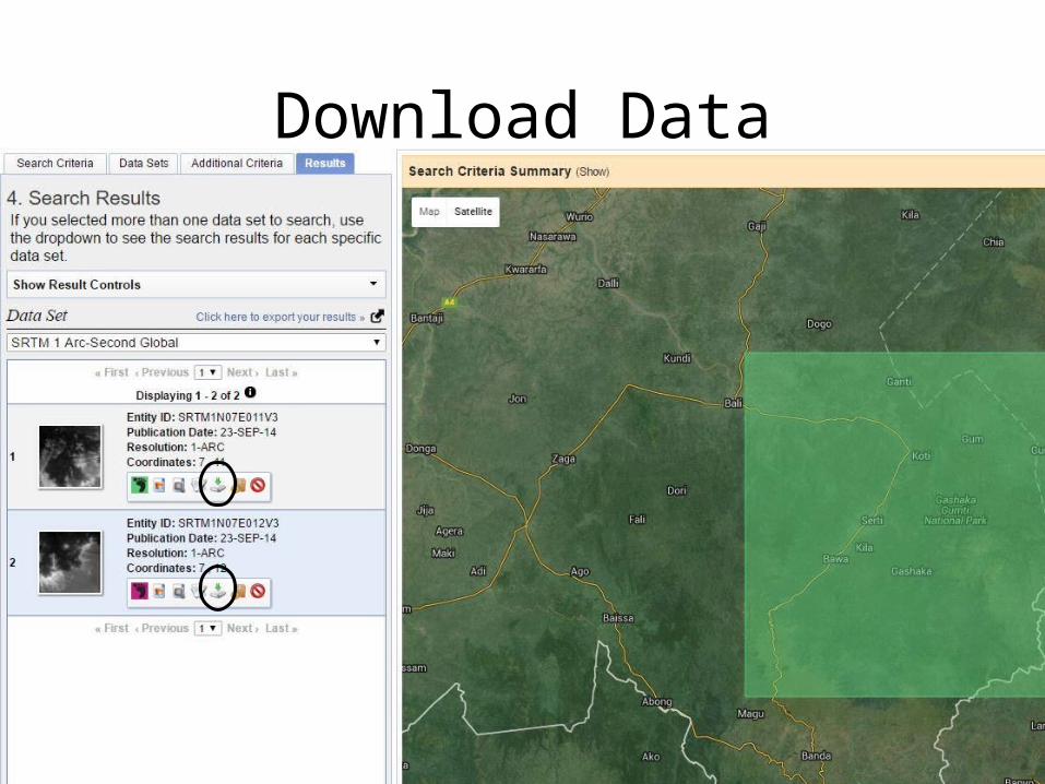
• You can show the SRTM image footprints by using the buttons on the left.
• We see there are two SRTM images that fall within my AOI. • I will have to download both of them and mosaic (merge)
them into a new raster.• You can display metadata (SRTM files were collected in 2000
but published in 2014). You can do individual or bulk downloads.
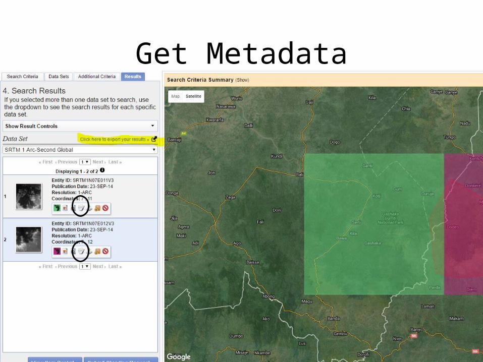
Get Metadata
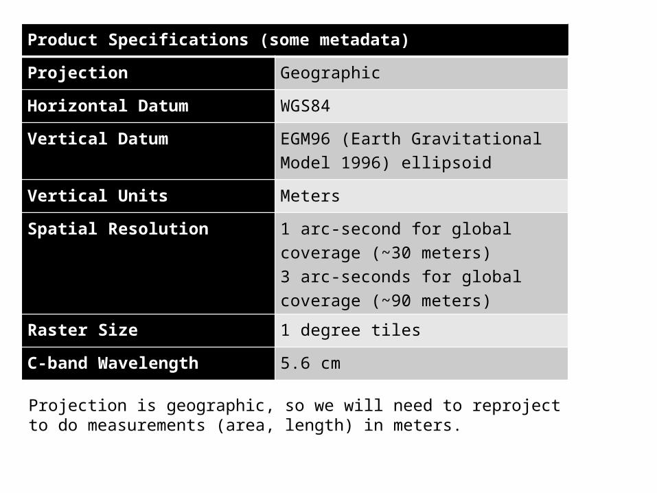
Product Specifications (some metadata)
Projection GeographicHorizontal Datum WGS84Vertical Datum EGM96 (Earth Gravitational
Model 1996) ellipsoid
Vertical Units MetersSpatial Resolution 1 arc-second for global coverage
(~30 meters)3 arc-seconds for global coverage (~90 meters)
Raster Size 1 degree tilesC-band Wavelength 5.6 cm
Projection is geographic, so we will need to reproject to do measurements (area, length) in meters.
Download Data
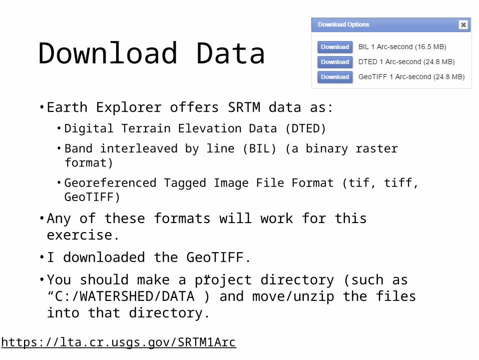
Download Data• Earth Explorer offers SRTM data as:
• Digital Terrain Elevation Data (DTED)• Band interleaved by line (BIL) (a binary raster format) • Georeferenced Tagged Image File Format (tif, tiff,
GeoTIFF) • Any of these formats will work for this exercise.• I downloaded the GeoTIFF.• You should make a project directory (such as
“C:/WATERSHED/DATA”) and move/unzip the files into that directory.
https://lta.cr.usgs.gov/SRTM1Arc
2. Set Work Environment
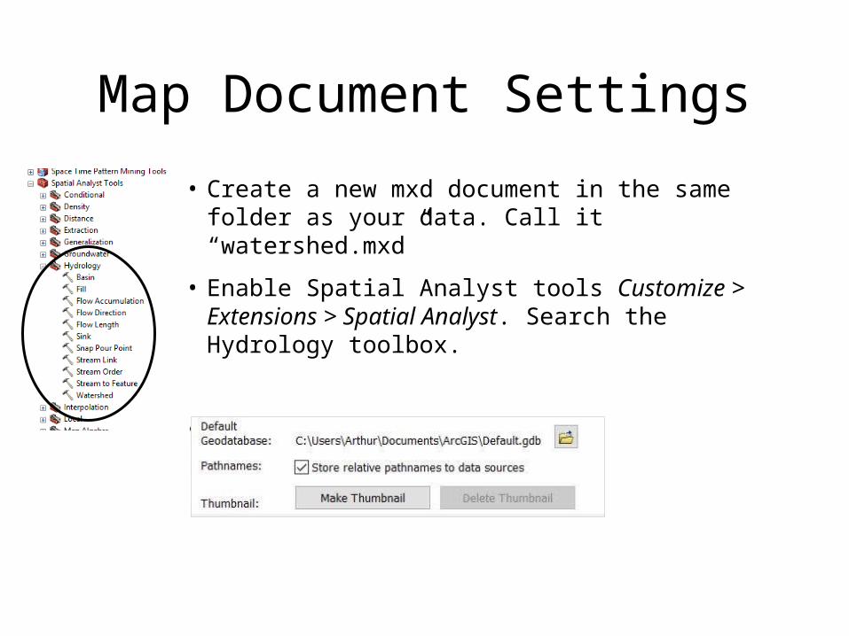
Map Document Settings• Create a new mxd document in the same folder
as your data. Call it “watershed.mxd”• Enable Spatial Analyst tools Customize >
Extensions > Spatial Analyst. Search the Hydrology toolbox.
• Set Map Document Properties
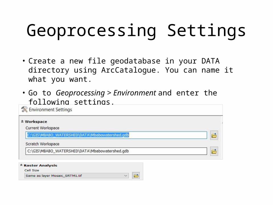
Geoprocessing Settings• Create a new file geodatabase in your DATA directory
using ArcCatalogue. You can name it what you want. • Go to Geoprocessing > Environment and enter the
following settings.
Load Data and Check Properties
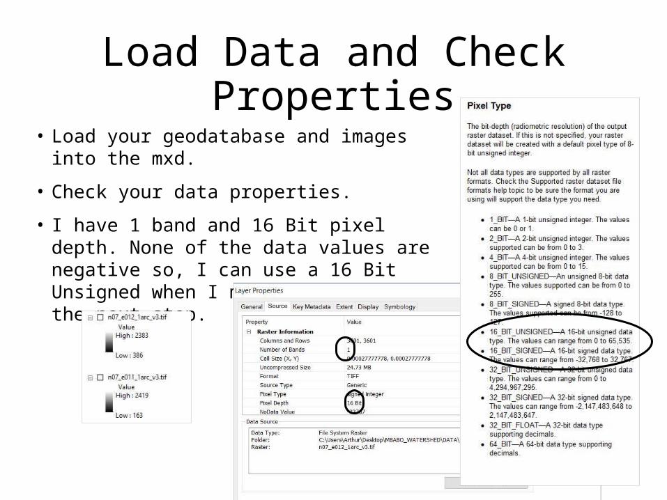
• Load your geodatabase and images into the mxd.
• Check your data properties.• I have 1 band and 16 Bit pixel depth.
None of the data values are negative so, I can use a 16 Bit Unsigned when I mosaic rasters in the next step.
3. Mosaic Rasters
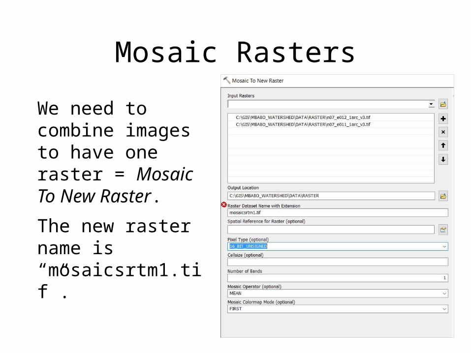
Mosaic RastersWe need to combine images to have one raster = Mosaic To New Raster.The new raster name is “mosaicsrtm1.tif”.
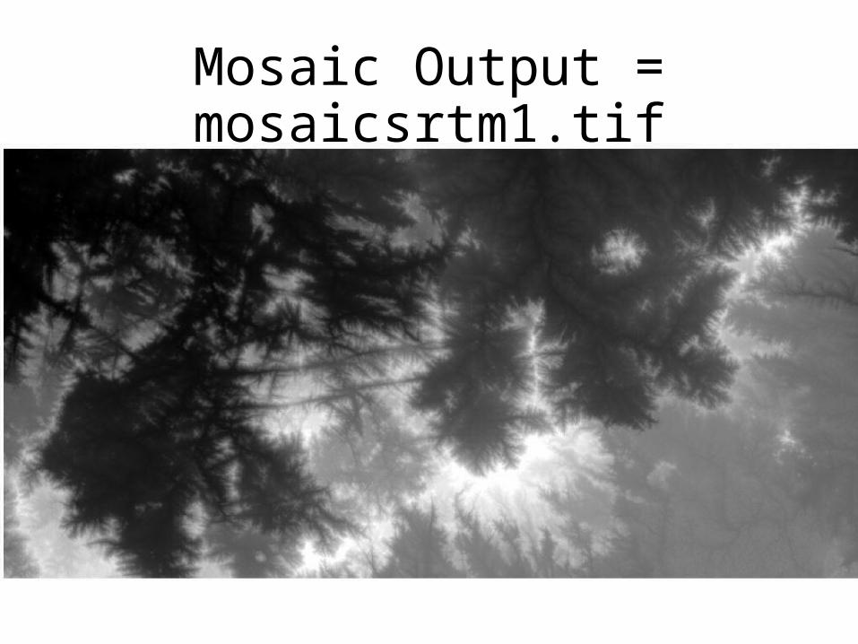
Mosaic Output = mosaicsrtm1.tif
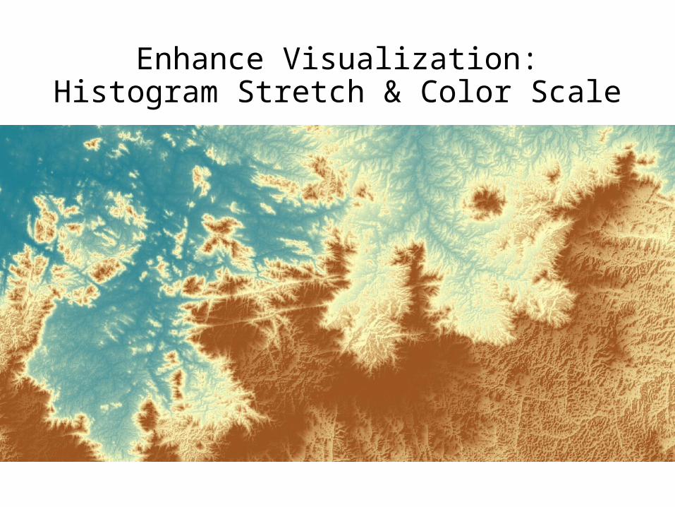
Enhance Visualization: Histogram Stretch & Color Scale
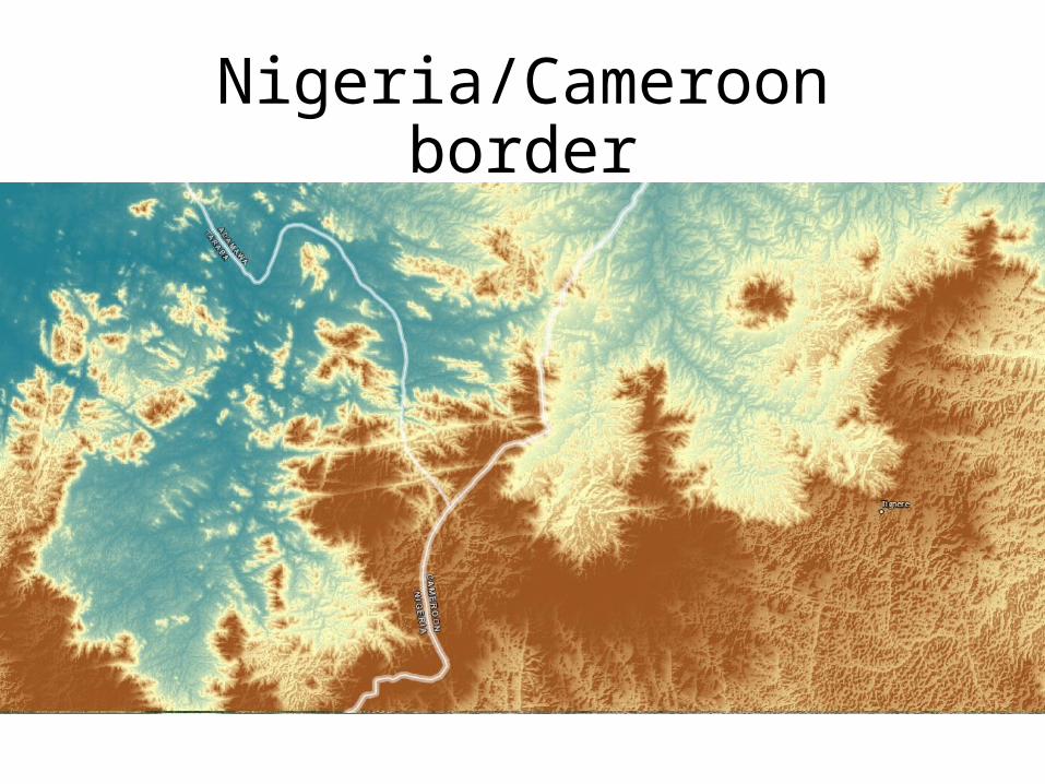
Nigeria/Cameroon border
4. Find Sinks & Fill Sinks
(Creating a depressionless DEM)
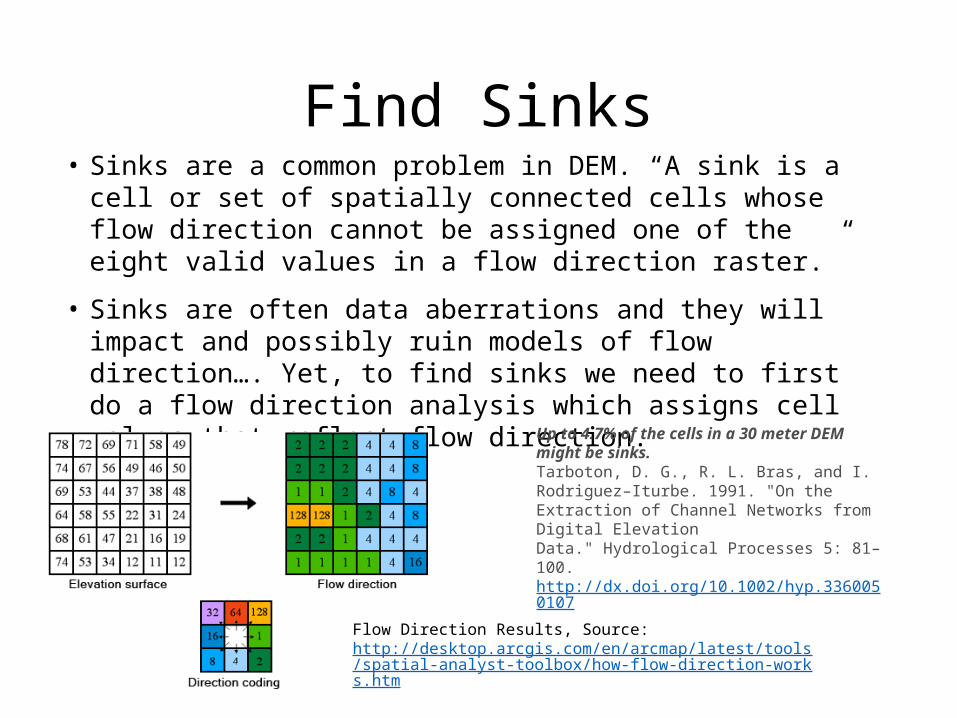
Find Sinks• Sinks are a common problem in DEM. “A sink is a cell or
set of spatially connected cells whose flow direction cannot be assigned one of the eight valid values in a flow direction raster.”
• Sinks are often data aberrations and they will impact and possibly ruin models of flow direction…. Yet, to find sinks we need to first do a flow direction analysis which assigns cell values that reflect flow direction.
Flow Direction Results, Source: http://desktop.arcgis.com/en/arcmap/latest/tools/spatial-analyst-toolbox/how-flow-direction-works.htm
Up to 4.7% of the cells in a 30 meter DEM might be sinks.Tarboton, D. G., R. L. Bras, and I. Rodriguez–Iturbe. 1991. "On the Extraction of Channel Networks from Digital Elevation Data." Hydrological Processes 5: 81–100. http://dx.doi.org/10.1002/hyp.3360050107
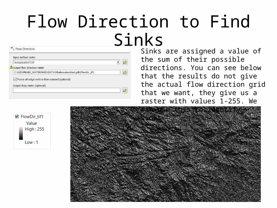
Flow Direction to Find Sinks
Sinks are assigned a value of the sum of their possible directions. You can see below that the results do not give the actual flow direction grid that we want, they give us a raster with values 1-255. We can use this to identify sinks.
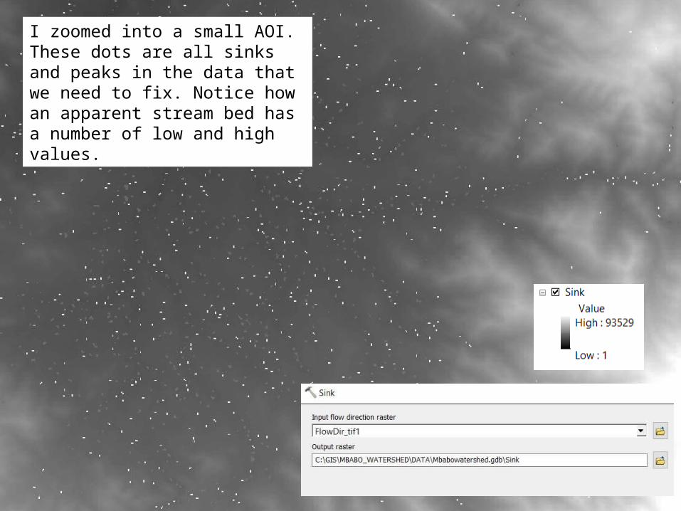
I zoomed into a small AOI. These dots are all sinks and peaks in the data that we need to fix. Notice how an apparent stream bed has a number of low and high values.
Fill
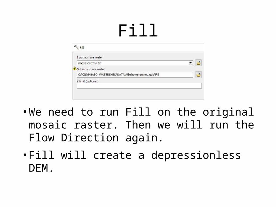
• We need to run Fill on the original mosaic raster. Then we will run the Flow Direction again.• Fill will create a depressionless DEM.
5. Flow Direction
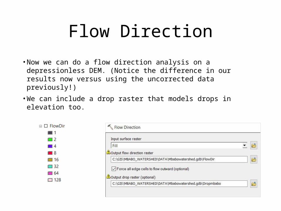
Flow Direction• Now we can do a flow direction analysis on a
depressionless DEM. (Notice the difference in our results now versus using the uncorrected data previously!)
• We can include a drop raster that models drops in elevation too.
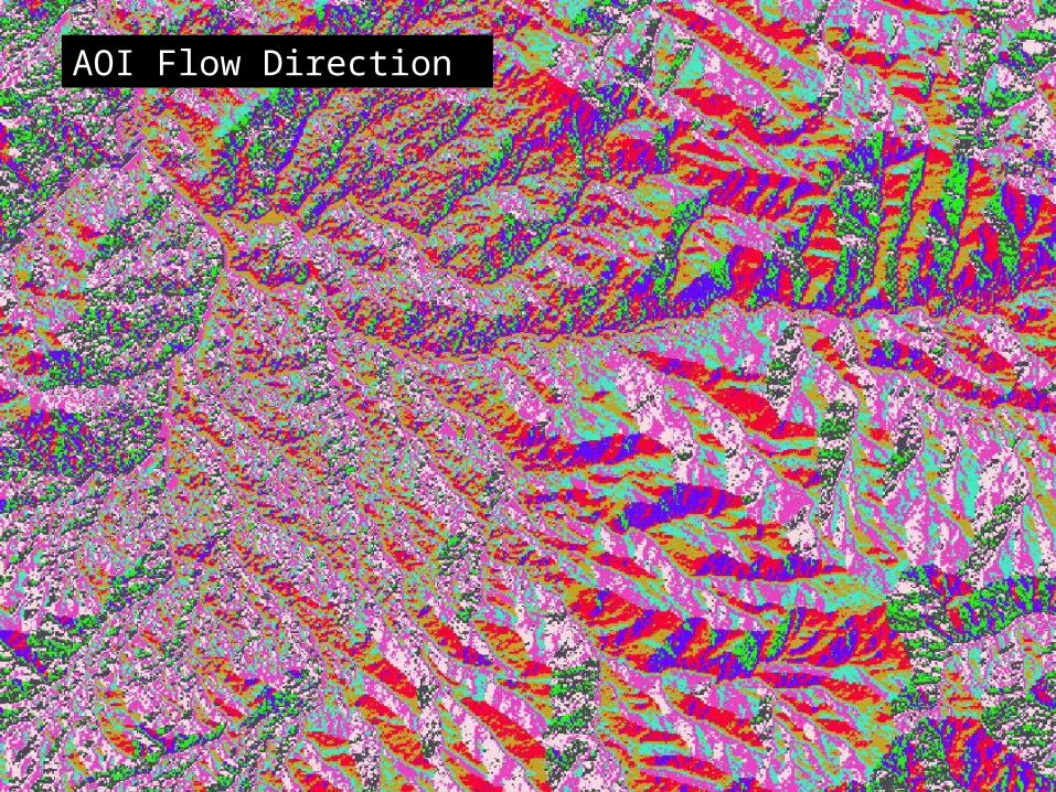
AOI Flow Direction
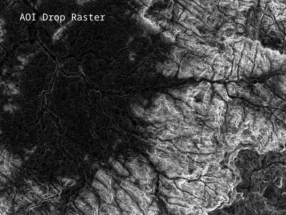
AOI Drop Raster
6. Flow Accumulation
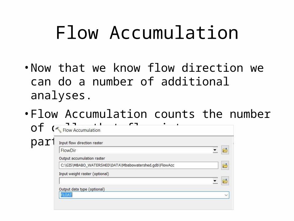
Flow Accumulation• Now that we know flow direction we can
do a number of additional analyses. • Flow Accumulation counts the number of
cells that flow into a particular cell.
Flow Accumulation
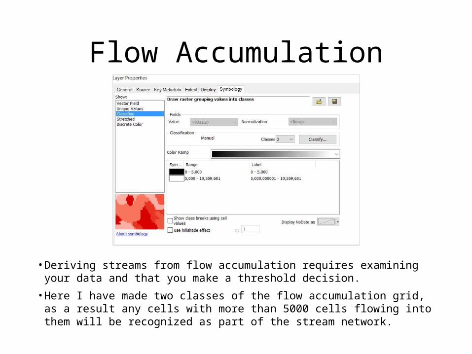
• Deriving streams from flow accumulation requires examining your data and that you make a threshold decision.
• Here I have made two classes of the flow accumulation grid, as a result any cells with more than 5000 cells flowing into them will be recognized as part of the stream network.
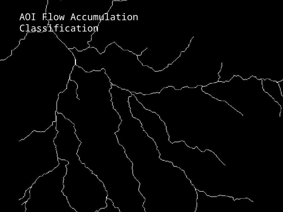
AOI Flow Accumulation Classification
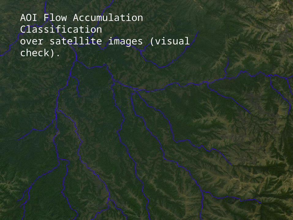
AOI Flow Accumulation Classificationover satellite images (visual check).
6. Basins and Watersheds
Basins and Watersheds• There is a function (Basin) that will
automatically calculate the basins in your data set using flow direction.• There is a way for us to choose to model
specific watersheds by establishing pour points and looking at flow accumulation. • Let’s look at how to do both of these and
then compare our results. Watersheds will take longer, so let’s start by making basins.
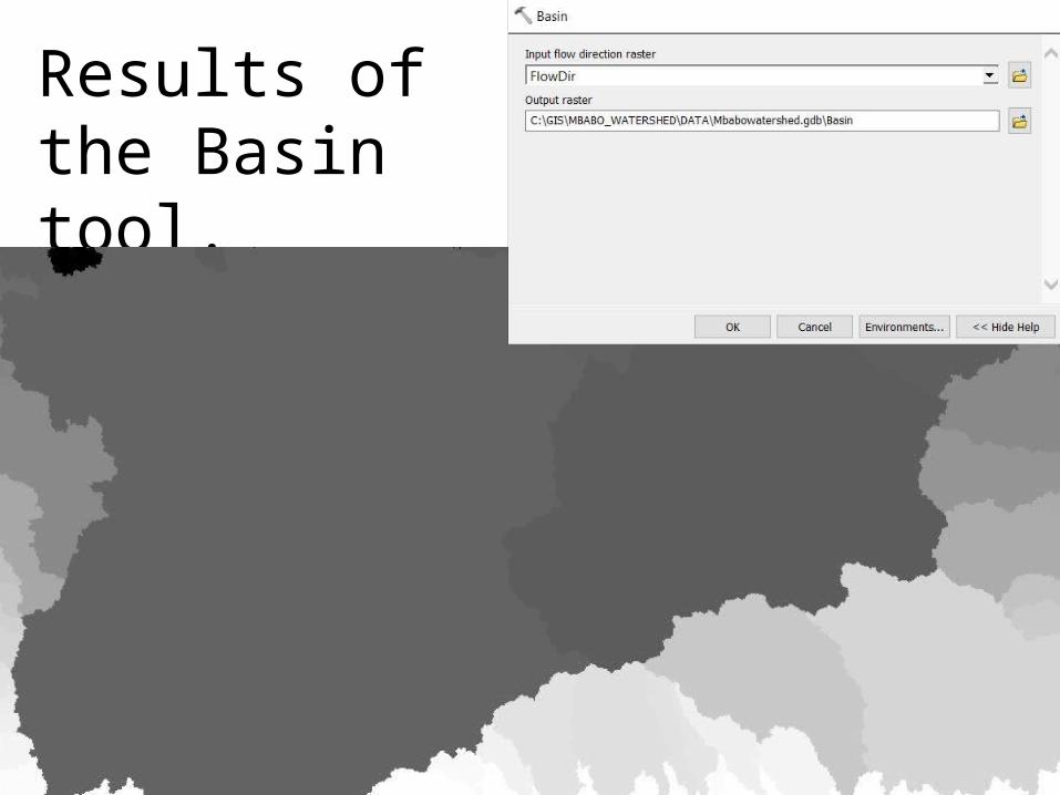
Results of the Basin tool.
Watersheds• Pour points are outlets of the watershed
that you are interested in mapping. • You can upload a predetermined set of
pour points (based on known locations) or you can establish your own set of points.• You will first need to create an empty
shapefile (or geodatabase feature class) for your points. You can do this in ArcCatalogue. Call the new layer “pourpoints”.
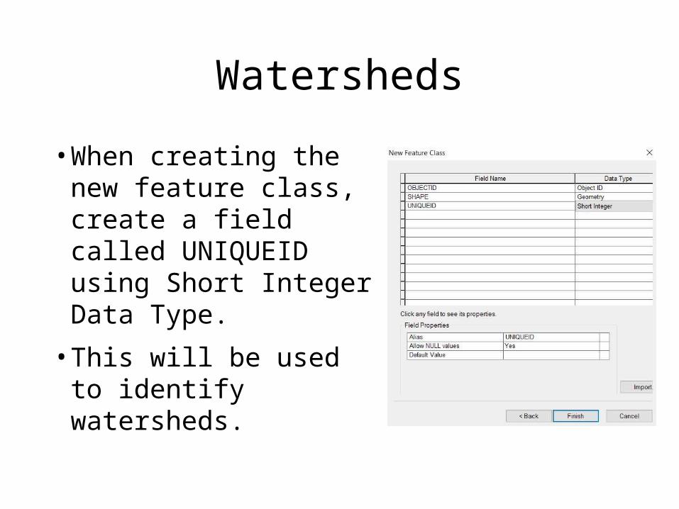
Watersheds• When creating the new
feature class, create a field called UNIQUEID using Short Integer Data Type.• This will be used to
identify watersheds.
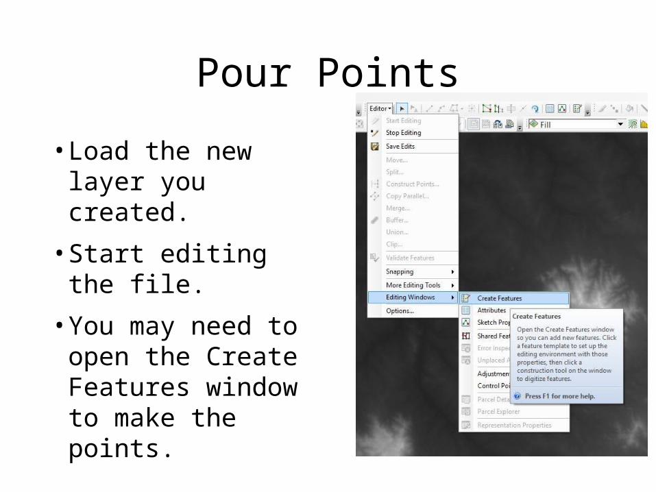
Pour Points• Load the new layer
you created.• Start editing the
file.• You may need to
open the Create Features window to make the points.
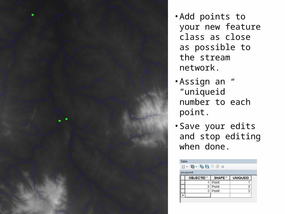
• Add points to your new feature class as close as possible to the stream network.• Assign an
“uniqueid” number to each point.• Save your edits
and stop editing when done.
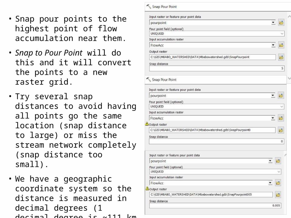
• Snap pour points to the highest point of flow accumulation near them.
• Snap to Pour Point will do this and it will convert the points to a new raster grid.
• Try several snap distances to avoid having all points go the same location (snap distance to large) or miss the stream network completely (snap distance too small).
• We have a geographic coordinate system so the distance is measured in decimal degrees (1 decimal degree is ~111 km at the equator but changes further from the equator).
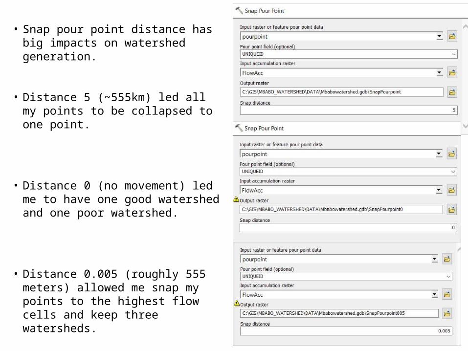
• Snap pour point distance has big impacts on watershed generation.
• Distance 5 (~555km) led all my points to be collapsed to one point.
• Distance 0 (no movement) led me to have one good watershed and one poor watershed.
• Distance 0.005 (roughly 555 meters) allowed me snap my points to the highest flow cells and keep three watersheds.
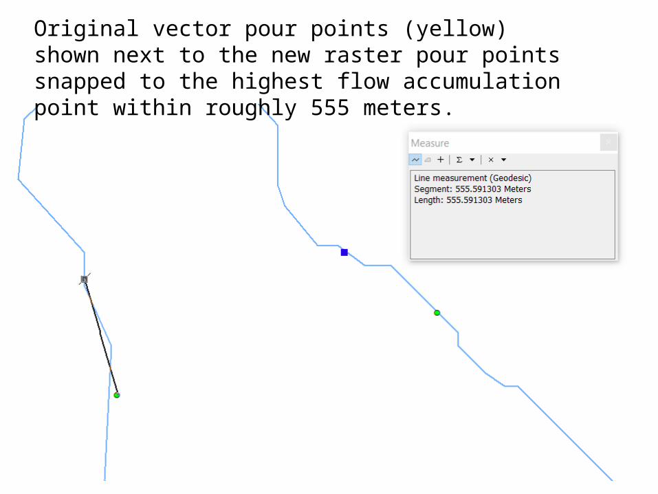
Original vector pour points (yellow) shown next to the new raster pour points snapped to the highest flow accumulation point within roughly 555 meters.
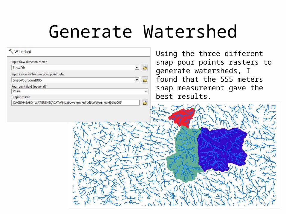
Generate WatershedUsing the three different snap pour points rasters to generate watersheds, I found that the 555 meters snap measurement gave the best results.
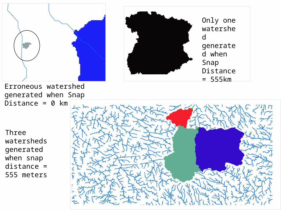
Erroneous watershed generated when Snap Distance = 0 km
Only one watershed generated when Snap Distance = 555km
Three watersheds generated when snap distance = 555 meters

7. Stream Network
Creating a Stream Network• In order to get our raster streams into a
vector format and to perform some other analysis, we need to make a raster that only shows our streams.• We will use Raster Calculator (located in
the toolbox Spatial Analyst > Map Algebra).• Use the formula on the following slide to
generate a new raster with only the streams represented.
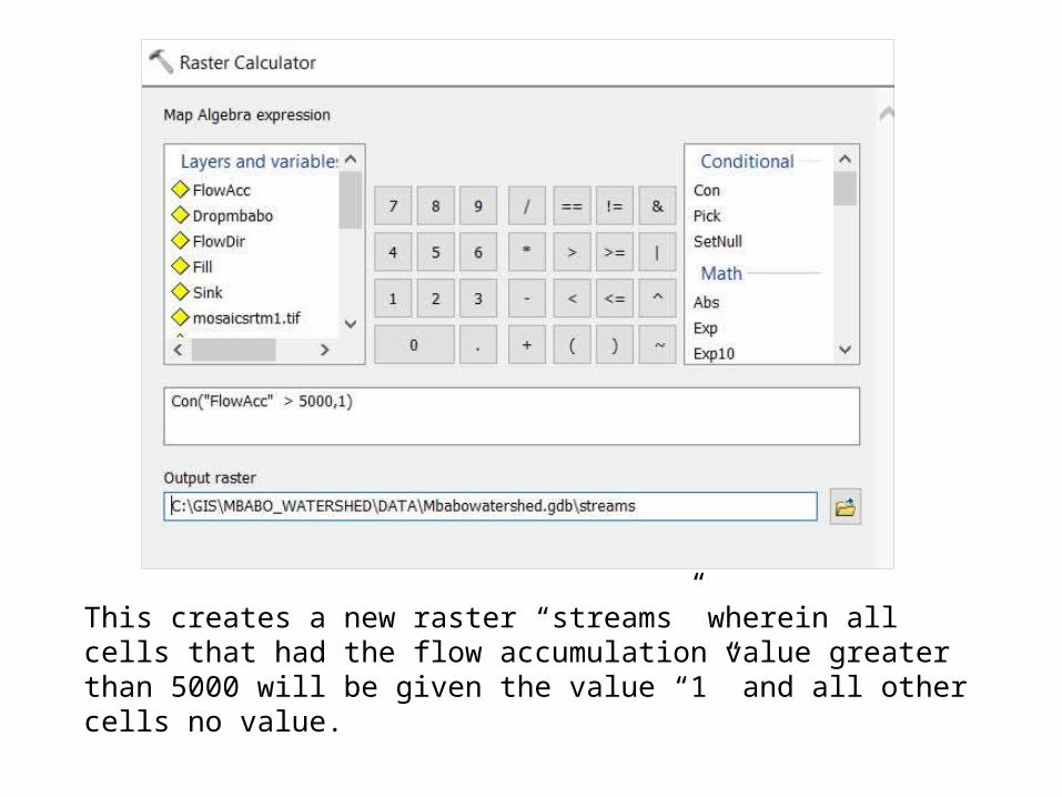
This creates a new raster “streams” wherein all cells that had the flow accumulation value greater than 5000 will be given the value “1” and all other cells no value.

Creating a Stream NetworkLinear raster stream network.
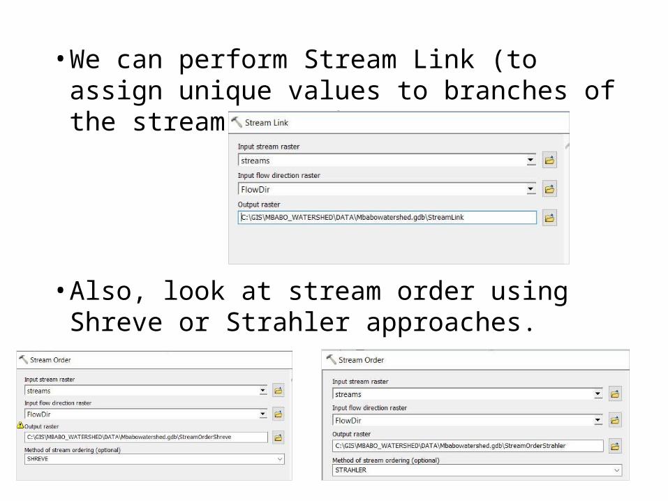
• We can perform Stream Link (to assign unique values to branches of the stream network).
• Also, look at stream order using Shreve or Strahler approaches.
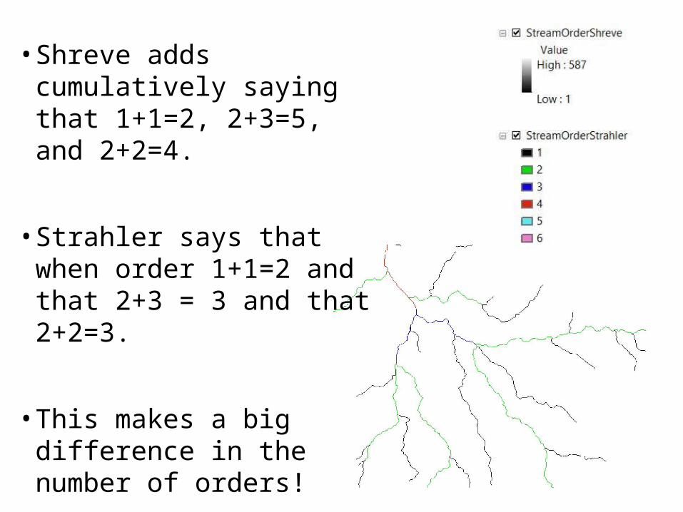
• Shreve adds cumulatively saying that 1+1=2, 2+3=5, and 2+2=4.
• Strahler says that when order 1+1=2 and that 2+3 = 3 and that 2+2=3.
• This makes a big difference in the number of orders!
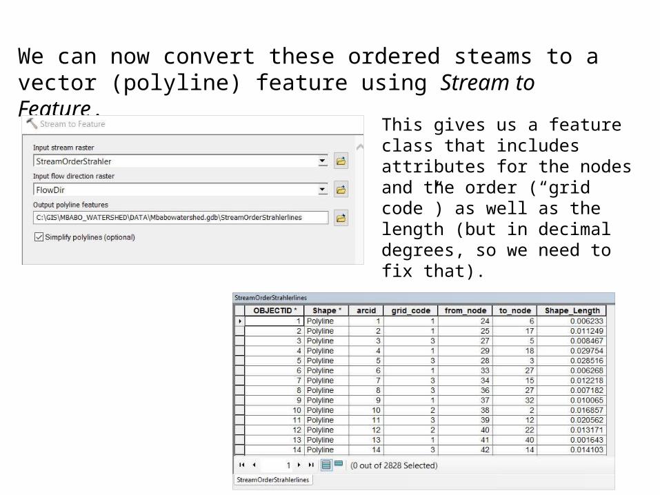
We can now convert these ordered steams to a vector (polyline) feature using Stream to Feature.
This gives us a feature class that includes attributes for the nodes and the order (“grid code”) as well as the length (but in decimal degrees, so we need to fix that).
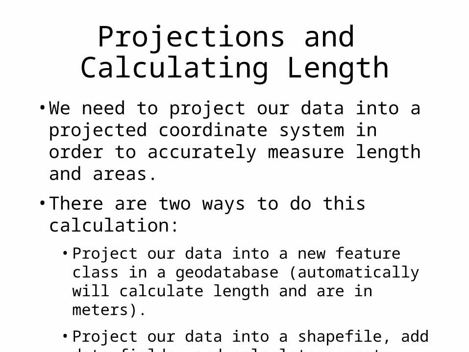
Projections and Calculating Length
• We need to project our data into a projected coordinate system in order to accurately measure length and areas. • There are two ways to do this calculation:• Project our data into a new feature class in a
geodatabase (automatically will calculate length and are in meters). • Project our data into a shapefile, add data
fields, and calculate geometry for the new fields.
Projections• First find a projected coordinate system
that is appropriate. • For my data I used UTM Zone 33N (which
covers the majority of my region). • I add the EPSG number to the file name to
identify the projection. The EPSG for UTM Zone 33N is 32633.• You can reproject direcly to a feature
class (gdb) or a shapefile.
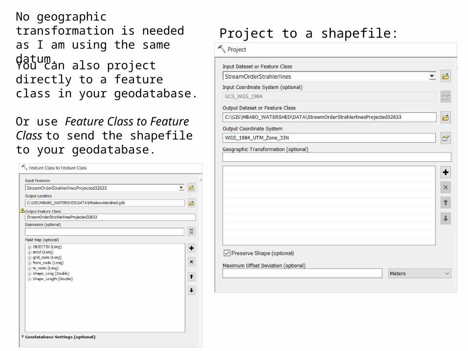
You can also project directly to a feature class in your geodatabase.
Or use Feature Class to Feature Class to send the shapefile to your geodatabase.
Project to a shapefile:No geographic transformation is needed as I am using the same datum.
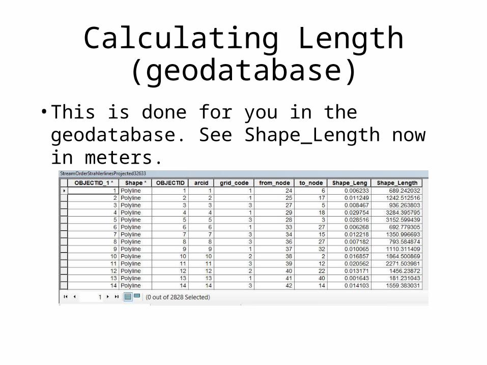
Calculating Length (geodatabase)
• This is done for you in the geodatabase. See Shape_Length now in meters.
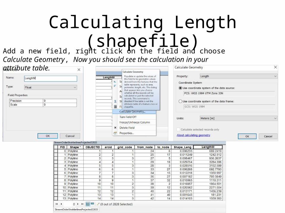
Calculating Length (shapefile)
Add a new field, right click on the field and choose Calculate Geometry, Now you should see the calculation in your attribute table.
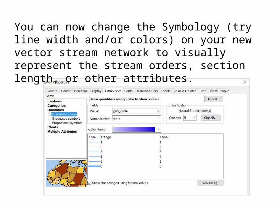
You can now change the Symbology (try line width and/or colors) on your new vector stream network to visually represent the stream orders, section length, or other attributes.
9. Converting to Polygons and Cleaning Up
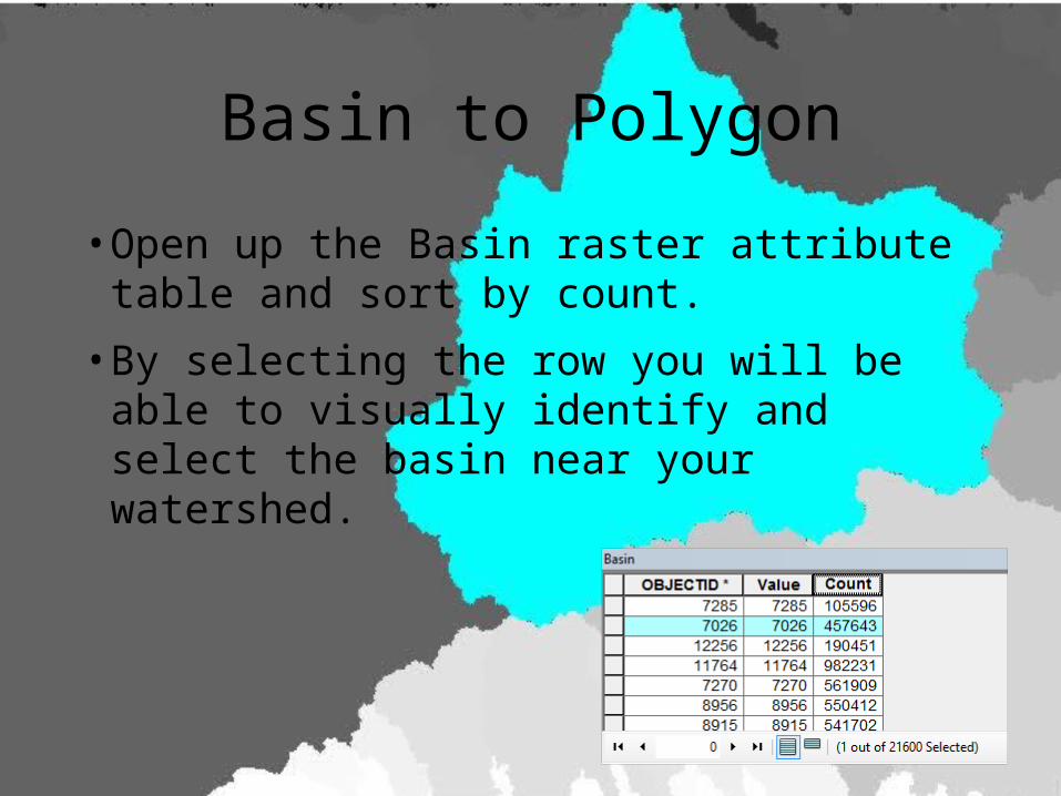
Basin to Polygon• Open up the Basin raster attribute table
and sort by count.• By selecting the row you will be able to
visually identify and select the basin near your watershed.
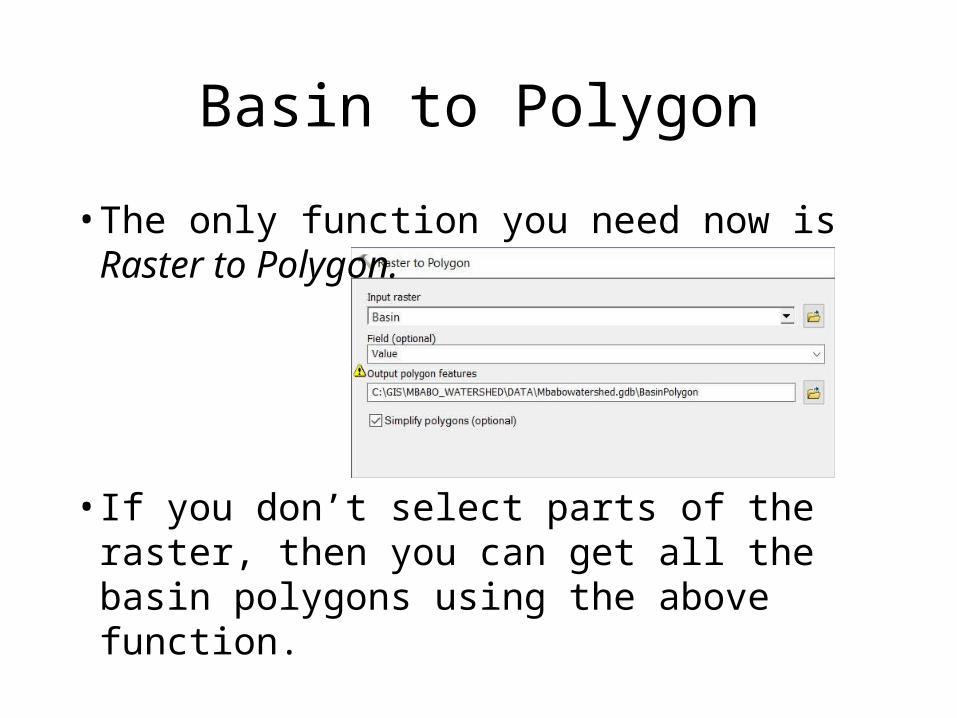
Basin to Polygon• The only function you need now is Raster
to Polygon.
• If you don’t select parts of the raster, then you can get all the basin polygons using the above function.
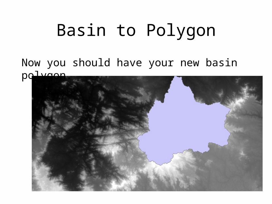
Basin to PolygonNow you should have your new basin polygon.
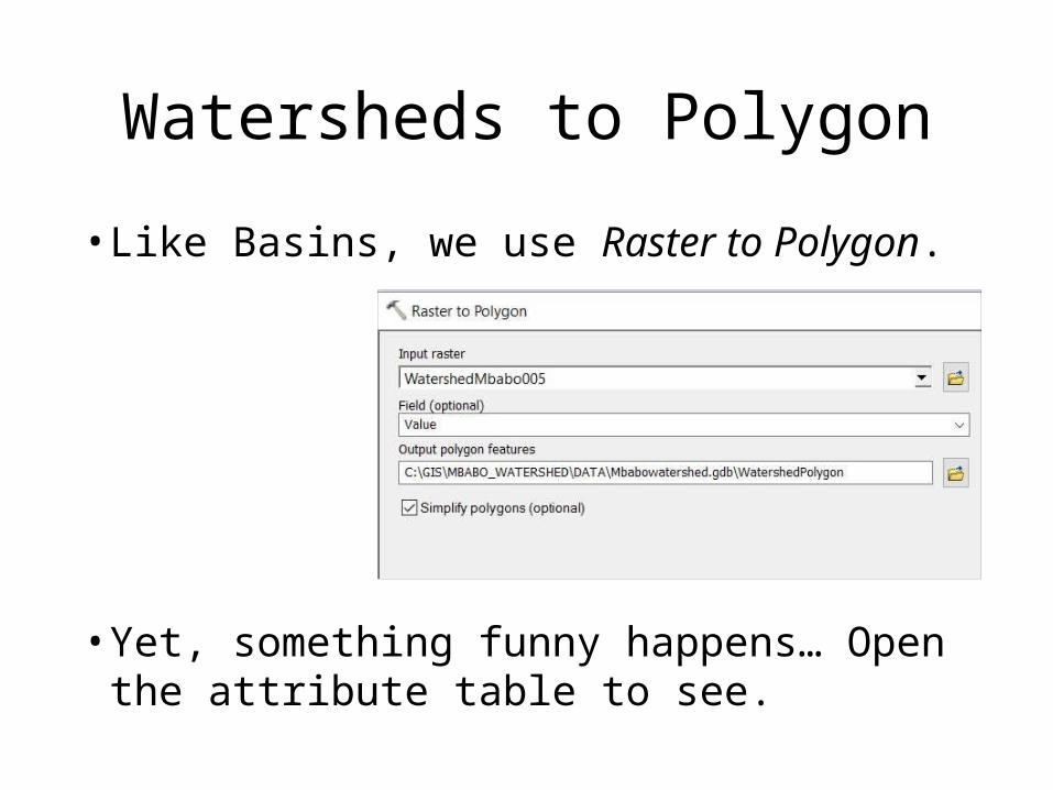
Watersheds to Polygon• Like Basins, we use Raster to Polygon.
• Yet, something funny happens… Open the attribute table to see.
Watersheds to Polygon
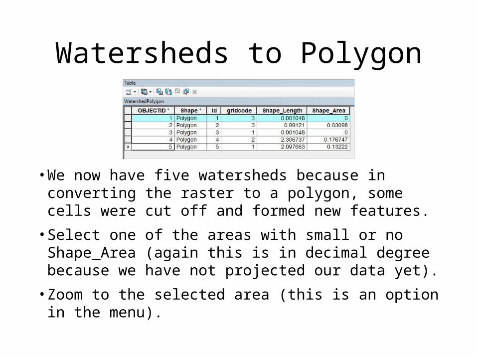
• We now have five watersheds because in converting the raster to a polygon, some cells were cut off and formed new features.• Select one of the areas with small or no
Shape_Area (again this is in decimal degree because we have not projected our data yet).• Zoom to the selected area (this is an option in the
menu).
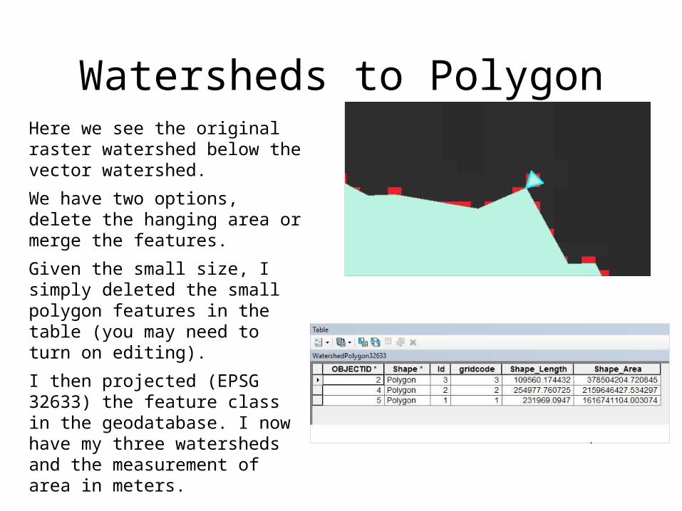
Watersheds to PolygonHere we see the original raster watershed below the vector watershed. We have two options, delete the hanging area or merge the features. Given the small size, I simply deleted the small polygon features in the table (you may need to turn on editing).I then projected (EPSG 32633) the feature class in the geodatabase. I now have my three watersheds and the measurement of area in meters.
10. Comparing Basin to Watersheds
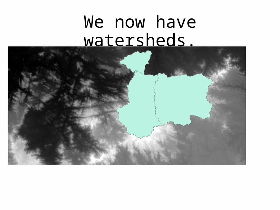
We now have watersheds.

We now have a basin and rivers.
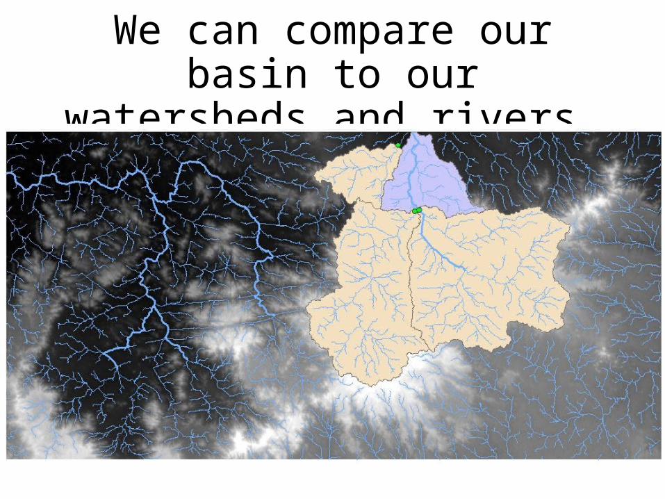
We can compare our basin to our watersheds and
rivers.
We can compare our basin to our watersheds and
rivers.• When we decided to locate pour points, we
ended up not capturing the entire basin and even including part of another basin. • This could impact field decisions.• For example, if we were collecting flow
information with monitors located in the field we might decide to change the location of our pour points (monitors) to more accurately represent the entire basin and maybe even capture 1-2 more basins with the same amount of monitors.

11. Answering the Research Question
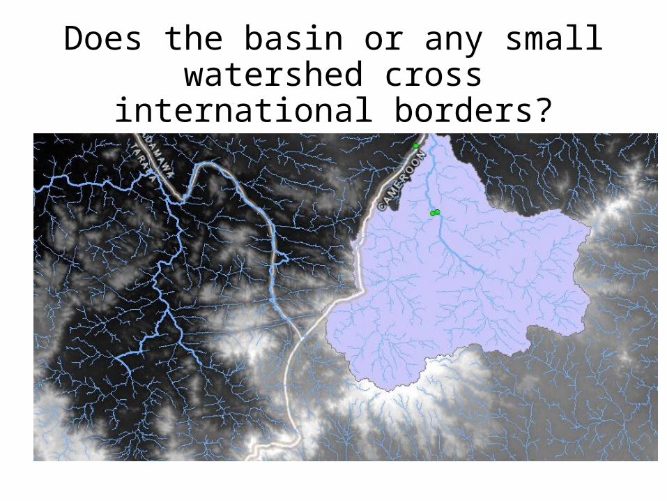
Does the basin or any small watershed cross international
borders?
Does the basin or any small watershed cross international
borders?• Yes, the basin appears to cross the border, it is largely in
Cameroon with small parts of it in Nigeria. • As well there were other basins that, appeared to cross
the border (largely in Nigeria with small parts in Cameroon).
• We could continue on with this analysis identifying and quantifying the overlap of basins throughout this region.
• Given our findings, we might suggest that the basin and watersheds overlapping the border are reasons to explore an international conservation area or an international agreement on watershed management.
Looking BackYou now know how to:
• Get SRTM 1 Arc-Second (30 meter resolution) for free.• Merge raster grids into mosaics. • Derive streams, stream orders, basins, and specific
watersheds from the data. • Convert raster grids into vector features. • Calculate area and length. • Create and analyze evidence for responding to
geographic questions. More information about this region can be found from organizations such as BirdLife International: http://www.birdlife.org/datazone/sitefactsheet.php?id=6112
EndDid you find an error?
Could something be more clearly explained? Did you adopt and adapt these materials?
Let me know at [email protected]
Watershed Delineation by Arthur Gill Green is licensed under a Creative Commons Attribution-ShareAlike 4.0 International License.
Based on a work at http://greengeographer.com/.