water conservation and residential landscapes: household...

Journal of Agricultural and Resource Economics 3 l(2): 173-192 Copyright 2006 Western Agricultural Economics Association

Water Conservation and Residential Landscapes: Household Preferences,

Household Choices

Brian H. Hurd

Communities throughout the Western United States are challenged by tight water supplies and swellingpopulations. Information is needed to better develop and target municipal water conservation programs. Significant water savings ranging from 35% to 70% are possible from changes in residential landscaping and improved management of outside watering, which often accounts for more than 50% of total residential water use. This study examines landscape choices of homeowners in three cities in New Mexico in order to identify and measure behavioral factors affecting water conservation. Using survey data, landscape choices are analyzed with a mixed logit model that assesses the effects of landscape and homeowner characteristics on choice probabilities. Model coefficients and implied elasticities indicate that water cost, education, and regional culture are significant determinants of landscape choice. In addition, the results suggest moral suasion can also have a positive influence toward water-conserving landscapes.

Key words: discrete choice, landscape preferences, New Mexico water, residential landscape, water conservation, water conservation programs, water savings

Introduction

Water conservation is a prominent issue challenging communities throughout the Western United States. States and local governments are grappling with the design and development ofwater conservation plans and strategies that will permit continued economic development in the face of limited and, in some cases, dwindling water resources. In the New Mexico S ta te Water Plan, for example, it states:

The Office of the State Engineer will encourage local governments and water providers to develop and implement comprehensive water conservation plans and will recommend that a water conservation plan be required in any application for State financial assistance for water development infrastructure (New Mexico Office of the State Engineer, Interstate Stream Commission, 2003).

Brian H. Hurd is assistant professor, Department of Agricultural Economics and Agricultural Business, New Mexico State University, Las Cmces. The author gratefully acknowledgesNew Mexico State University's Agricultural Experiment Station for its continued research support, and the Rio Grande Basin Initiative--a joint research program of New Mexico State University (NMSU) and Texas A&M University-for funding this project. Special appreciation is extended to the following individuals for their assistance during the course of this project: Josh Smith and Sylvia Beuhler for their research assistance and help in coordinating the survey; John White, Rolston St. Hilaire, Rhonda Skaggs, and Bernd Leinauer for technical assistance and review; Joshua Rosenblatt of the City of Las Cruces for his enthusiasm and stimulating insights; Craig Runyan and Leeann DeMouche for their overall project leadership and support; and the survey participants and water conservation staff from the cities of Albuquerque, Santa Fe, and Las Cmces, New Mexico. Finally, my thanks also go to two anonymous reviewers who contributed to the paper's clarity and presentation.

Review coordinated by Paul M. Jakus.

174 August 2006 Journal of Agricultural and Resource Economics

Similar laws exist in other states, such as Colorado (Colorado Water Conservation Board, 2005).

As public resources are directed into water conservation programs, local governments and utility managers are concerned about program effectiveness and the means to measure program outcomes and performance. Assessments of public attitudes and behavioral changes can provide both quantitative and qualitative measures of the impacts of water conservation programs and their effectiveness. A key challenge, therefore, is designing an approach and instrument to measure such changes and to track responses as water conservation programs develop and mature.

At its core, water conservation combines awareness of water sources and services and an understanding of how behavioral changes can enhance the value of these services. Central to the problem of designing effective water conservation programs-and hence to long-term planning of urban water resources-is the question of how responsive individuals and households are to various types of water conservation incentives. Allowing for heterogeneity, the question is also how households with certain characteristics are responsive to program characteristics and incentives.

This study uses data collected in 2004 from a mail survey of homeowners in three New Mexico cities who provided responses indicating their attitudes toward landscape and water use (Hurd and Smith, 2005). The survey and data are briefly summarized and are then used in a discrete choice, random utility model in order to measure the sensitivity and responsiveness of landscape choices to changes in conservation program incentives such as water price and moral suasion, and to examine how these responses differ with changes in individual and household characteristics.

Water Conservation and Landscape Choice

Residential demand for water is growing rapidly throughout the West and is creating pressure for new sources of domestic water supplies. The economic literature on urban water demand is quite extensive and is only briefly addressed here. A central aspect of this literature has focused on behavioral changes in water use and, in particular, on the sensitivity of water use to changes in prices, income, and conservation policies. Approaches for estimating urban water demands have confronted many methodological issues, including consumer perception of prices (Nieswiadomy, 1992), complexities in rate structures (Nieswiadomy and Molina, 1989,1991; Hewitt and Hanemann, 1995), and seasonal use patterns (Lyman, 1992; Nieswiadomy, 1992; Espey, Espey, and Shaw, 1997; Dalhuisen et al., 2003).

Though differences may exist in the use of particular methods or models, a consistent finding confirms the relatively low sensitivity of residential water demand to price changes. Inelastic demands are common with estimates rangingfrom -0.26 to -0.75, as observed by Espey, Espey, and Shaw (1997) in a meta-analysis of 24 studies on urban water demands. Even more recently, Dalhuisen et al. (2003) examined results from 64 studies and found that increasing block rate price policies (e.g., where the unit price rises in increments as quantity rises) do lead to greater consumer sensitivity and higher price elasticities. Reviewing urban residential water data and analyses, Brookshire et al. (2002) argue for water pricing institutions that reflect scarcity and lead to more efficient water use and allocation.

Hurd Water Conservation and Residential Landscapes 175

Some studies have attempted to account for the effects of local water conservation programs. A dummy variable specification was used by both Nieswiadomy (1992) and Taylor, McKean, and Young (2004), and no measurable effect was found on estimated urban water demands, although Nieswiadomy reported that public education in the West had a measurable effect. Shaw and Maidment (1988) concluded that voluntarypro- grams had little effect on water use. By developing a more varied approach and including the type and number of program elements (e.g., education programs, appliance retrofit, public information), Michelsen, McGuckin, and Stumpf (1999) found significant reductions of between 1% and 4% in water demand per program element across seven South- western cities. However, none of the program elements focused on outdoor water use and, in particular, landscape water use.

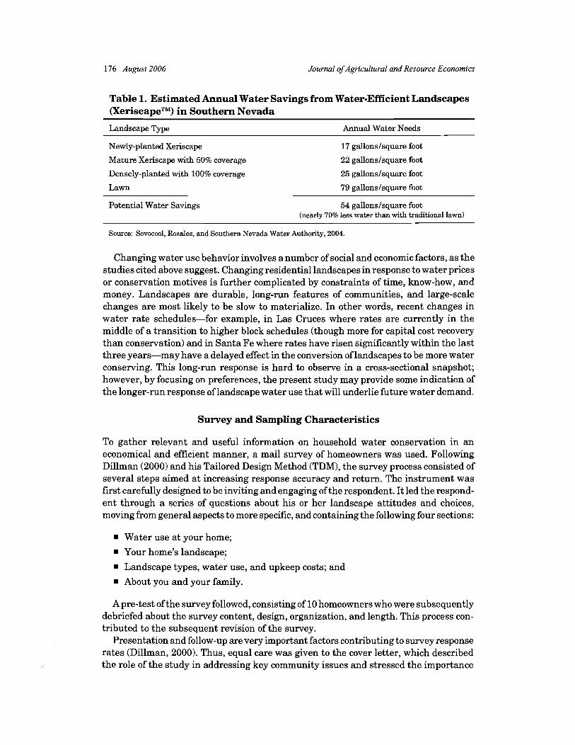
Throughout the arid and semi-arid regions of the Western United States, watering residential landscapes is the single greatest household use of water. Often accounting for more than 50% of household annual water consumption, landscape irrigation is a major component of per capita water use throughout the West. Typically, cities with the highest levels of per capita water use are dominated by residential areas with traditional turfgrass landscapes and hydrophilic landscapes. By altering outdoor water use patterns, significant water savings may be possible (as shown in table I), with estimates ranging from 35% to 75% of current per capita water use based on a typical home with a traditional bluegrass type landscape (Ferguson, 1987; Knopf, 2003; Sovocool, Rosales, and Southern Nevada Water Authority, 2004h1

Landscape choices and changes are prompted by many factors including water price, awareness of water scarcity and drought concerns, perceived aesthetic attributes, landscapes of neighbors, municipal codes, and the time, effort, and cost of making changes. A central concern and question is whether and to what extent can the quality of life derived from a home's landscape be enhanced while a t the same time using less water.

Along the Rio Grande, throughout the arid West, and even in increasingly water- scarce areas in the East, water-intensive lawn landscapes are beginning to give way to more water-efficient and climate-appropriate landscapes. For example, Spinti, St. Hilare, and VanLeeuwen (2004) describe the acceptability of desert-type landscapes for homeowners in Las Cruces, New Mexico. Their findings revealed an increasing acceptance of the aesthetics of desert-type landscapes-i.e., more than 80% of respondents for use in front yards, and greater than 56% in back yards; however, they found that actual adoption rates were lower by 25% to 30%. One of the central concerns addressed in the present study is the extent to which there are differences in landscape preferences across different communities.

' It is important to note, however, that achieved rates of water savings will depend on factors beyond simply exchanging one type of vegetation for another. Arguably more important than vegetation type is the system of irrigation used and the capability of the homeowner to effectively manage the system forwater efficiency. Researchersat the University of California, Riverside, Turfgrass Research Facility, for example, have estimated that two-thirds of the water savings from municipal turf rebate programs is the result of upgraded and more efficient irrigation systems, while the remaining one-third is attributable to the switch from turfgrass to XeriscapeTM, a term coined by Denver Water in the 1980s (Addink, 2005). In some cases, researchers have found higher water use (by as much as 10%) for Xeriscape compared to traditional landscapes. The researchers attribute this to several factors including pruning management and high planting densities, and water management regimes to encourage rapid growth. "Drought-tolerant species can tolerate drought ... but they grow slowly under droughty conditions and often are less aesthetically pleasing. What this means in terms of water management is that xeriphytic landscapes can induce residents to use more water than they would with traditional landscapes" (Addink, 2005, p. 4). Landscape choice is important, but achieving successful water savings requires efficient irrigation systems, properly installed and managed.


Table 1. Estimated Annual Water Savings from Water-Efficient Landscapes (XeriscapeTM) in Southern Nevada

Landscape Type Annual Water Needs

Newly-planted Xeriscape 17 gallons/square foot

Mature Xeriscape with 50% coverage 22 gallons/square foot

Densely-planted with 100% coverage 25 gallons/square foot

Lawn 79 gallons/square foot

Potential Water Savings 54 gallons/square foot (nearly 70% less water than with traditional lawn)

Source: Sovocool, Rosales, and Southern Nevada Water Authority, 2004.

Changing water use behavior involves a number of social and economic factors, as the studies cited above suggest. Changing residential landscapes in response to water prices or conservation motives is further complicated by constraints of time, know-how, and money. Landscapes are durable, long-run features of communities, and large-scale changes are most likely to be slow to materialize. In other words, recent changes in water rate schedules-for example, in Las Cruces where rates are currently in the middle of a transition to higher block schedules (though more for capital cost recovery than conservation) and in Santa Fe where rates have risen significantly within the last three years-may have a delayed effect in the conversion of landscapes to be more water conserving. This long-run response is hard to observe in a cross-sectional snapshot; however, by focusing on preferences, the present study may provide some indication of the longer-run response of landscape water use that will underlie future water demand.

Survey and Sampling Characteristics

To gather relevant and useful information on household water conservation in an economical and efficient manner, a mail survey of homeowners was used. Following Dillman (2000) and his Tailored Design Method (TDM), the survey process consisted of several steps aimed at increasing response accuracy and return. The instrument was first carefully designed to be inviting and engaging of the respondent. It led the respondent through a series of questions about his or her landscape attitudes and choices, moving from general aspects to more specific, and containing the following four sections:

Water use at your home;

Your home's landscape;

m Landscape types, water use, and upkeep costs; and

About you and your family.

A pre-test of the survey followed, consisting of 10 homeowners who were subsequently debriefed about the survey content, design, organization, and length. This process contributed to the subsequent revision of the survey.

Presentation and follow-up are very important factors contributing to survey response rates (Dillman, 2000). Thus, equal care was given to the cover letter, which described the role of the study in addressing key community issues and stressed the importance


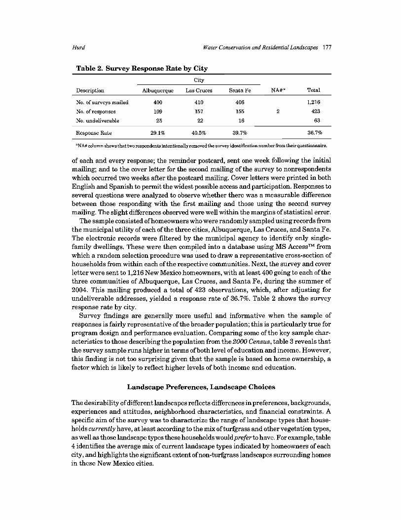
Table 2. Survey Response Rate by City

City

Description Albuquerque Las Cruces Santa Fe NA# " Total

No. of surveys mailed 400 410 406 1,216

No. of responses 109 157 155 2 423

No. undeliverable 25 22 16 63

Response Rate 29.1% 40.5% 39.7% 36.7%

'NA# column shows that two respondents intentionally removed the survey identification number from their questionnaire.

of each and every response; the reminder postcard, sent one week following the initial mailing; and to the cover letter for the second mailing of the survey to nonrespondents which occurred two weeks after the postcard mailing. Cover letters were printed in both English and Spanish to permit the widest possible access and participation. Responses to several questions were analyzed to observe whether there was a measurable difference between those responding with the first mailing and those using the second survey mailing. The slight differences observed were well within the margins of statistical error.

The sample consisted of homeowners who were randomly sampled using records from the municipal utility of each of the three cities, Albuquerque, Las Cruces, and Santa Fe. The electronic records were filtered by the municipal agency to identify only single- family dwellings. These were then compiled into a database using MS AccessTM from which a random selection procedure was used to draw a representative cross-section of households from within each of the respective communities. Next, the survey and cover letter were sent to 1,216 New Mexico homeowners, with at least 400 going to each of the three communities of Albuquerque, Las Cruces, and Santa Fe, during the summer of 2004. This mailing produced a total of 423 observations, which, after adjusting for undeliverable addresses, yielded a response rate of 36.7%. Table 2 shows the survey response rate by city.

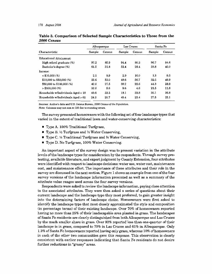
Survey findings are generally more useful and informative when the sample of responses is fairly representative of the broader population; this is particularly true for program design and performance evaluation. Comparing some of the key sample characteristics to those describing the population from the 2000 Census, table 3 reveals that the survey sample runs higher in terms of both level of education and income. However, this finding is not too surprising given that the sample is based on home ownership, a factor which is likely to reflect higher levels of both income and education.

Landscape Preferences, Landscape Choices

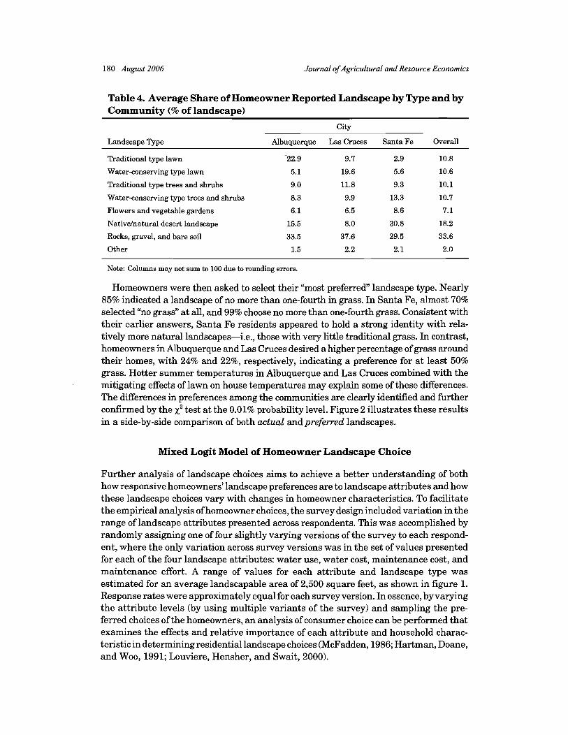
The desirability of different landscapes reflects differences in preferences, backgrounds, experiences and attitudes, neighborhood characteristics, and financial constraints. A specific aim of the survey was to characterize the range of landscape types that households currently have, a t least according to the mix of turfgrass and other vegetation types, as well as those landscape types these households wouldprefer to have. For example, table 4 identifies the average mix of current landscape types indicated by homeowners of each city, and highlights the significant extent of non-turfgrass landscapes surrounding homes in these New Mexico cities.


Table 3. Comparison of Selected Sample Characteristics to Those from the 2000 Census

Albuquerque Las Cruces Santa Fe

Characteristic Sample Census Sample Census Sample Census

Educational Attainment:

High school graduate (%) 97.2 85.9 94.4 80.3 96.7 84.6

Bachelor's degree (%) 61.5 31.8 52.4 28.4 59.8 40.0

Income:

< $10,000 (%) 2.1 9.9 2.9 16.0 1.3 9.5

$10,000 to $50,000 (%) 23.6 53.0 48.6 56.7 32.5 49.9

$50,000 to $100,000 (%) 42.0 27.5 38.2 22.6 44.3 28.9

> $100,000 (%) 32.0 9.6 9.6 4.6 21.5 11.8

Households ~Dndividuals Aged < 18 40.6 33.3 19.1 33.8 30.1 26.8

Households ~Dndividuals Aged > 65 24.3 20.7 45.4 23.4 27.5 23.1

Sources: Author's data and U.S. Census Bureau, 2000 Census of the Population. Note: Columns may not sum to 100 due to rounding errors.

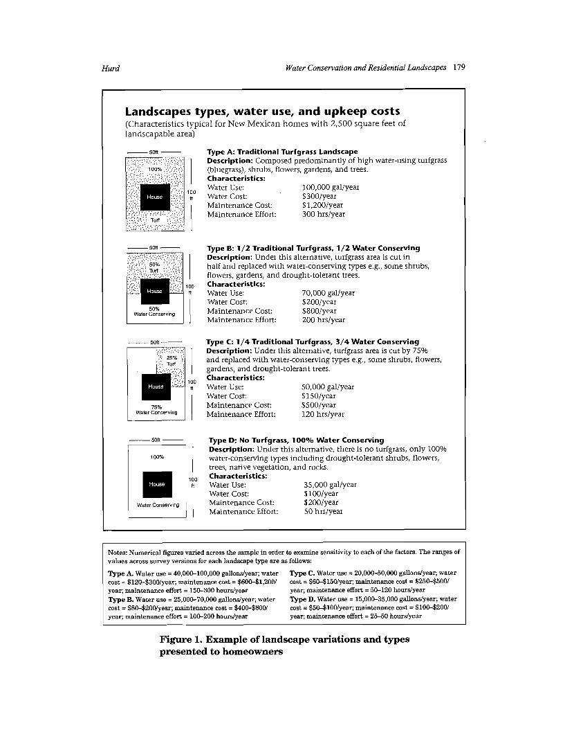
The survey presented homeowners with the following set of four landscape types that varied in the extent of traditional lawn and water-conserving characteristics:

Type A. 100% Traditional Turfgrass,

Type B. 1/2 Turfgrass and 1/2 Water Conserving,

Type C. ?4 Traditional Turfgrass and %i Water Conserving,

Type D. No Turfgrass, 100% Water Conserving.

An important aspect of the survey design was to present variation in the attribute levels of the landscape types for consideration by the respondents. Through survey pre- testing, available literature, and expert judgment by County Extension, four attributes were identified with respect to landscape decisions: water use, water cost, maintenance cost, and maintenance effort. The importance of these attributes and their role in the survey are discussed in the next section. Figure 1 shows an example from one of the four survey versions of the landscape information presented as well as a summary of the attribute value ranges used across the four survey versions.

Respondents were asked to review the landscape information, paying close attention to the associated attributes. They were then asked a series of questions about their current landscape and the landscape type they most preferred, to gain greater insight into the determining factors of landscape choice. Homeowners were first asked to identify the landscape type that most closely approximated the style and composition (in percentage terms) of their existing landscape. Over 70% of homeowners reported having no more than 25% of their landscapable area planted in grass. The landscapes of Santa Fe residents are clearly distinguished from both Albuquerque and Las Cruces by the much smaller share in grass. Over 93% reported less than one-quarter of their landscape is in grass, compared to 70% in Las Cruces and 61% in Albuquerque. Only 1.3% of Santa Fe homeowners reported having only grass, whereas 10% of homeowners in each of the other two communities gave this response. This observation is clearly consistent with earlier responses indicating that Santa Fe residents do not desire further reductions in "grassy" areas.


Landscapes types, water use, and upkeep costs (Characteristics typical for New Mexican homes with 2,500 square feet of landscapable area)

water-using turfgrass

Characteristics: Water Use: 100,000 gallyear

$300/year Maintenance Cost: $1,20O/year Maintenance Effort: 300 hrslyear

- 5ofi - Type B: 1/2 Traditional Turfgrass, 1/2 Water Conserving Description: Under this alternative, turfgrass area is cut in half and replaced with water-conserving types e.g., some shrubs, flowers, gardens, and drought-tolerant trees. Characteristics:

fi Water Use: 70,000 gallyear Water Cost: $200/year Maintenance Cost: $800/year Maintenance Effort: 200 hrslyear

Type C: 1 /4 Traditional Turfgrass, 3/4 Water Conserving Description: Under this alternative, turfgrass area is cut by 75% and replaced with water-conserving types e.g., some shrubs, flowers, gardens, and drought-tolerant trees.

100 Characteristics:

fl Water Use: 50,000 gallyear Water Cost: $150/year Maintenance Cost: $500/year

Water Conserving Maintenance Effort: 120 hrslyear

- 5011- Type D: No Turfgrass, 100% Water Conserving Description: Under this alternative, there is no turfgrass, only 100%

100% water-conserving types including drought-tolerant shrubs, flowers, trees, native vegetation, and rocks.

loo Characteristics: fi Water Use: 35,000 gallyear

Water Cost: $100/year Water Conserving Maintenance Cost: $200/year

Maintenance Effort: 50 hrslyear

Notes: Numerical figures varied across the sample in order to examine sensitivity to each of the factors. The ranges of values across survey versions for each landscape type are as follows:

Type A. Water use = 40,000-100,000 gallonsfyear; water Type C. Water use = 20,000-50,000 gallonsfyear; water cost = $120-$300lyear; maintenance cost = $600-$1,2001 cost = $60-$150lyear; maintenance cost = $250-$5001 year; maintenance effort = 150-300 hourdyear year; maintenance effort = 50-120 hourdyear Type B. Water use = 25,000-70,000 gallondyear; water Type D. Water use = 15,000-35,000 gallondyear; water cost = $80-$2001year; maintenance cost = $400-$8001 cost = $50-$lOOlyear; maintenance cost = $100-$2001 year; maintenance effort = 100-200 hourdyear year; maintenance effort = 25-50 howdyear

Figure 1. Example of landscape variations and types presented to homeowners


Table 4. Average Share of Homeowner Reported Landscape by Type and by Community (% of landscape)

City

Landscape Type Albuquerque Las Cruces Santa Fe Overall

Traditional type lawn

Water-conserving type lawn

Traditional type trees and shrubs

Water-conserving type trees and shrubs

Flowers and vegetable gardens

Nativelnatural desert landscape

Rocks, gravel, and bare soil

Other

Note: Columns may not sum to 100 due to rounding errors.

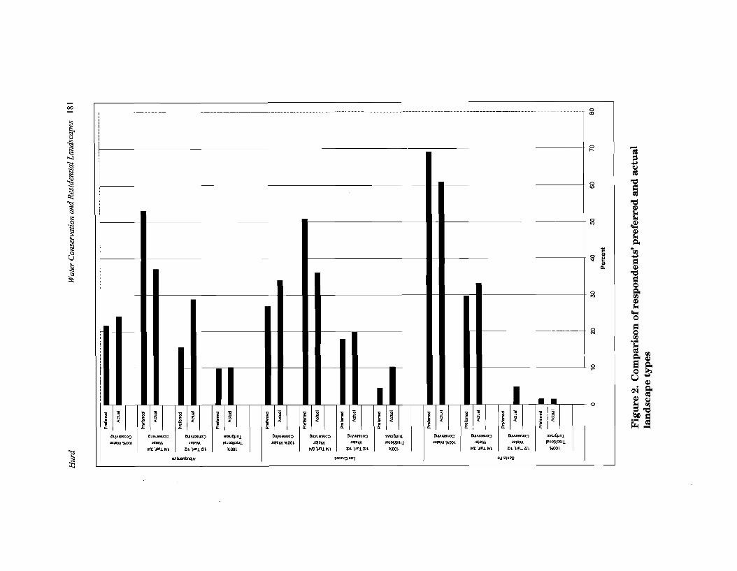
Homeowners were then asked to select their "most preferred" landscape type. Nearly 85% indicated a landscape of no more than one-fourth in grass. In Santa Fe, almost 70% selected "no grass" at all, and 99% choose no more than one-fourth grass. Consistent with their earlier answers, Santa Fe residents appeared to hold a strong identity with relatively more natural landscapes-i.e., those with very little traditional grass. In contrast, homeowners in Albuquerque and Las Cruces desired a higher percentage of grass around their homes, with 24% and 22%, respectively, indicating a preference for at least 50% grass. Hotter summer temperatures in Albuquerque and Las Cruces combined with the mitigating effects of lawn on house temperatures may explain some of these differences. The differences in preferences among the communities are clearly identified and further confirmed by the x2 test at the 0.01% probability level. Figure 2 illustrates these results in a side-by-side comparison of both actual and preferred landscapes.

Mixed Logit Model of Homeowner Landscape Choice

Further analysis of landscape choices aims to achieve a better understanding of both how responsive homeowners' landscape preferences are to landscape attributes and how these landscape choices vary with changes in homeowner characteristics. To facilitate the empirical analysis of homeowner choices, the survey design included variation in the range of landscape attributes presented across respondents. This was accomplished by randomly assigning one of four slightly varying versions of the survey to each respondent, where the only variation across survey versions was in the set of values presented for each of the four landscape attributes: water use, water cost, maintenance cost, and maintenance effort. A range of values for each attribute and landscape type was estimated for an average landscapable area of 2,500 square feet, as shown in figure 1. Response rates were approximately equal for each survey version. In essence, by varying the attribute levels (by using multiple variants of the survey) and sampling the preferred choices of the homeowners, an analysis of consumer choice can be performed that examines the effects and relative importance of each attribute and household characteristic in determining residential landscape choices (McFadden, 1986; Hartman, Doane, and Woo, 1991; Louviere, Hensher, and Swait, 2000).

Hur

d W

ater

Con

serv

atio

n an

d R

esid

entia

l Lan

dsca

pes

18 1

I 1

1 Pr

nhtrr

sd

s P-

i i P

A

ctua

l Z

PS

s

8 '!

Pm

fene

d

9 0

Per

cen

t

Fig

ure

2.

Com

par

ison

of

resp

ond

ents

' pre

ferr

ed a

nd

act

ual

la

nd

scap

e ty

pes

182 August 2006 Journal ofAgricultura1 and Resource Economics

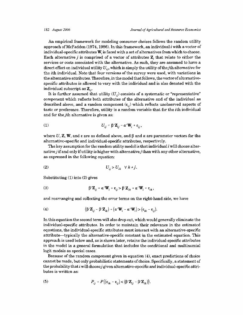
An empirical framework for modeling consumer choices follows the random utility approach of McFadden (1974,1986). In this framework, an individual i with a vector of individual-specific attributes Wi is faced with a set of alternatives from which to choose. Each alternative j is comprised of a vector of attributes Zj that relate to either the services or costs associated with the alternative. As such, they are assumed to have a direct effect on individual utility Uij, which is simply the utility of the jth alternative for the ith individual. Note that four versions of the survey were used, with variations in the alternative attributes. Therefore, in the model that follows, the vector of alternative- specific attributes is allowed to vary with the individual and is also denoted with the individual subscript as Z,,.

It is further assumed that utility (Uij) consists of a systematic or "representative" component which reflects both attributes of the alternative and of the individual as described above, and a random component (eij) which reflects unobserved aspects of taste or preference. Therefore, utility is a random variable that for the ith individual and for the jth alternative is given as:

where U, Z, W, and E are as defined above, and P and a are parameter vectors for the alternative-specific and individual-specific attributes, respectively.

The key assumption for the random utility model is that individual i will choose alternative j if and only if utility is higher with alternative j than with any other alternative, as expressed in the following equation:

Substituting (1) into (2) gives

p1zij + a'W, + E,, > PIZik + a1wi + Eik ,

and rearranging and collecting the error terms on the right-hand side, we have

In this equation the second term will also drop out, which would generally eliminate the individual-specific attributes. In order to maintain their relevance in the estimated equations, the individual-specific attributes must interact with an alternative-specific attribute-typically the alternative-specific constant in the estimated equation. This approach is used below and, as is shown later, retains the individual-specific attributes in the model in a general formulation that includes the conditional and multinomial logit models as special cases.

Because of the random component given in equation (4), exact predictions of choice cannot be made, but only probabilistic statements of choice. Specifically, a statement of the probability that i will choose j given alternative-specific and individual-specific attributes is written as:


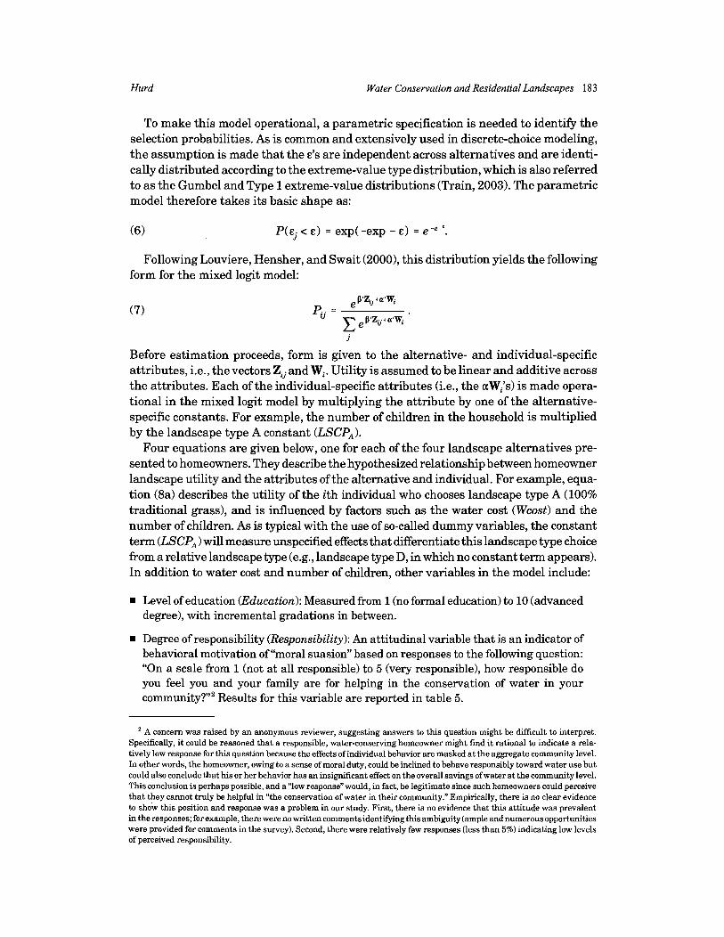
To make this model operational, a parametric specification is needed to identify the selection probabilities. As is common and extensively used in discrete-choice modeling, the assumption is made that the E'S are independent across alternatives and are identi- cally distributed according to the extreme-value type distribution, which is also referred to as the Gumbel and Type 1 extreme-value distributions (Train, 2003). The parametric model therefore takes its basic shape as:

Following Louviere, Hensher, and Swait (2000), this distribution yields the following form for the mixed logit model:

P'Z,, +a'Wi p.. =

41 ,p,zij+a,wi .

j

Before estimation proceeds, form is given to the alternative- and individual-specific attributes, i.e., the vectors Zi j and Wi. Utility is assumed to be linear and additive across the attributes. Each of the individual-specific attributes (i.e., the aW,'s) is made operational in the mixed logit model by multiplying the attribute by one of the alternative- specific constants. For example, the number of children in the household is multiplied by the landscape type A constant (LSCP,).

Four equations are given below, one for each of the four landscape alternatives presented to homeowners. They describe the hypothesized relationship between homeowner landscape utility and the attributes of the alternative and individual. For example, equation (8a) describes the utility of the ith individual who chooses landscape type A (100% traditional grass), and is influenced by factors such as the water cost (Wcost) and the number of children. As is typical with the use of so-called dummy variables, the constant tenn (LSCP, will measure unspecified effects that differentiate this landscape type choice from a relative landscape type (e.g., landscape type D, in which no constant term appears). In addition to water cost and number of children, other variables in the model include:

Level of education (Education): Measured from 1 (no formal education) to 10 (advanced degree), with incremental gradations in between.

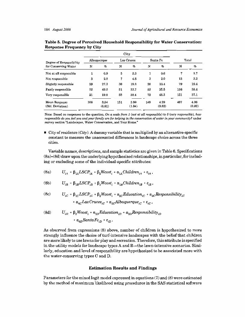
Degree of responsibility (Responsibility): An attitudinal variable that is an indicator of behavioral motivation of "moral suasion" based on responses to the following question: "On a scale from 1 (not at all responsible) to 5 (very responsible), how responsible do you feel you and your family are for helping in the conservation of water in your ~omrnunity?"~ Results for this variable are reported in table 5.

A concern was raised by an anonymous reviewer, suggesting answers to this question might be difficult to interpret. Specifically, it could be reasoned that a responsible, water-conserving homeowner might find it rational to indicate a relatively low response for this question because the effects of individual behavior are masked a t the aggregate community level. In other words, the homeowner, owing to a sense of moral duty, could be inclined to behave responsibly toward water use but could also conclude that his or her behavior has an insignificant effect on the overall savings ofwater at the community level. This conclusion is perhaps possible, and a "low responsen would, in fact, be legitimate since such homeowners could perceive that they cannot truly be helpful in "the conservation of water in their community." Empirically, there is no clear evidence to show this position and response was a problem in our study. First, there is no evidence that this attitude was prevalent in the responses; for example, there were no written commentsidentifying this ambiguity (ample and numerous opportunities were provided for comments in the survey). Second, there were relatively few responses (less than 5%) indicating low levels of perceived responsibility.


Table 5. Degree of Perceived Household Responsibility for Water Conservation: Response Frequency by City

City

Albuquerque Las Cmces Santa Fe Total Degree of Responsibility for Conserving Water N % N % N % N %

Not at all responsible 1 0.9 5 3.3 1 0.6 7 1.7

Not responsible 3 2.8 7 4.6 3 2.0 13 3.2

Slightly responsible 29 27.3 30 19.8 20 13.4 79 19.4

Fairly responsible 52 49.0 51 33.7 53 35.5 156 38.4

Very responsible 21 19.8 58 38.4 72 48.3 151 37.1

Mean Response 106 3.84 151 3.99 149 4.29 407 4.06 (Std. Deviation) (0.81) (1.04) (0.82) (0.92)

Note: Based on responses to the question, On a scale from 1 (not at all responsible) to 5 (very responsible), how responsible do you feel you and your family are for helping in the conservation of water in your community? under survey section "Landscapes, Water Conservation, and Your Home."

City of residence (City): A dummy variable that is multiplied by an alternative-specific constant to measure the unaccounted differences in landscape choice across the three cities.

Variable names, descriptions, and sample statistics are given in Table 6. Specifications (8a)-(8d) draw upon the underlying hypothesized relationships, in particular, for including or excluding some of the individual-specific attributes:

As observed from expressions (8) above, number of children is hypothesized to more strongly influence the choice of turf-intensive landscapes with the belief that children are more likely to use lawns for play and recreation. Therefore, this attribute is specified in the utility models for landscape types A and B-the lawn-intensive scenarios. Simi- larly, education and level of responsibility are hypothesized to be associated more with the water-conserving types C and D.

Estimation Results and Findings

Parameters for the mixed logit model expressed in equations (7) and (8) were estimated by the method of maximum likelihood using procedures in the SAS statistical software


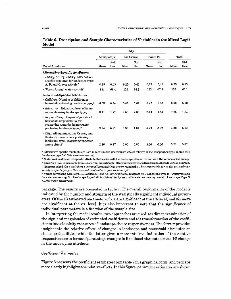
Table 6. Description and Sample Characteristics of Variables in the Mixed Logit Model

Model Attributes

Ci ty

Albuquerque Las Cmces Santa Fe Total

Std. Std. Std. Std. Mean Dev. Mean Dev. Mean Dev. Mean Dev.

Alternative-Specific Attributes:

b LSCP,, LSCP,, LSCP,: Alternative- specific constants for landscape types A, B, and C, respectively" 0.25 0.43 0.25 0.43 0.25 0.43 0.25 0.43

b Wcost: Annual water cost ($1 134 66.4 129 64.3 132 67.8 132 66.1

Individual-Specific Attributes:

b Children,: Number of children in households choosing landscape type j 0.68 0.94 0.41 1.07 0.47 0.83 0.50 0.96

b Education,: Education level of homeowner choosing landscape type j ' 8.11 1.77 7.65 2.03 8.14 1.64 7.95 1.84

Responsibility,: Degree of perceived household responsibility for conserving water by homeowners preferring landscape type j 3.84 0.81 3.99 1.04 4.29 0.82 4.06 0.92

City,: Albuquerque, Las Cruces, and Santa Fe homeowners preferring landscape type j (capturing variation across cities) ' 2.86 0.87 3.00 0.80 3.66 0.56 3.21 0.82

" Alternative-specific constants are used to measure the unaccounted effects relative to the nonspecified type, in this case landscape type D (100% water conserving).

Water cost is alternative-specific attribute that varies with the landscape alternative and with the version of the survey. 'Education level is measured from 1 (no formal education) to 10 (advanced degree), withincremental gradations in between.

Question asked: On a scale from 1 (not at all responsible) to 5 (very responsible), how responsible do you feel you and your family are for helping in the conservation of water in your community? " Values correspond as follows: 1 =Landscape Type A (100% traditional trufgrass); 2 = Landscape Type B (Yi turfgrass and Yi water conserving; 3 = Landscape Type C (?4 traditional turfgrass and % water conserving; and 4 = Landscape Type D (100% water conserving).

package. The results are presented in table 7. The overall performance of the model is indicated by the number and strength of the statistically significant individual parameters. Of the 13 estimated parameters, four are significant at the 1% level, and six more are significant at the 5% level. It is also important to note that the significance of individual parameters is a function of the sample size.

In interpreting the model results, two approaches are used: ( a ) direct examination of the sign and magnitudes of estimated coefficients and ( b ) transformation of the coefficients into elasticity measures of landscape choice responsiveness. The former provides insight into the relative effects of changes in landscape and household attributes on choice probabilities, while the latter gives a more intuitive indication of the relative responsiveness in terms of percentage changes in likelihood attributable to a 1% change in the underlying attribute.

Coefficient Estimates

Figure 3 presents the coefficient estimates from table 7 in a graphical form, and perhaps more clearly highlights the relative effects. In this figure, parameter estimates are shown


Table 7. Mixed Logit Model Parameter Estimates of Factors Influencing Residential Landscape Choice

Parameter Standard Chi Square Variable Estimate Error ( x 2 ) Pr > x2

LSCP, 6.290*** 2.066 9.272 0.002

LSCP, 5.688*** 1.875 9.199 0.002

LSCP, 5.245*** 1.819 8.314 0.004

Wcost -0.018** 0.008 4.935 0.026

Children, -0.823 0.888 0.859 0.354

Children, 0.309 0.188 2.699 0.100

Education, 0.298** 0.134 4.925 0.027

Education, 0.315** 0.148 4.563 0.033

Responsibility, 0.275 0.231 1.418 0.234

Responsibility, 0.706** 0.283 6.242 0.013

Las Cruces, -2.150** 1.073 4.014 0.045

Albuquerque, -2.124** 1.080 3.866 0.049

Santa Fe, 3.593*** 1.061 11.471 0.001

Likelihood Ratio Test: X2 = 160.3 [13 d.f.1; Pr > x2 = <0.0001

Note: Double and triple asterisks (*) denote statistical significance a t the 5% and 1% levels, respectively.

across each of the landscape types, which are shown moving from more water-conserving types (types D and C) to more water-intensive types (types B and A).

The signs of the parameter estimates are generally consistent with expectations. For example, the effect of water cost on the probability of landscape choice is increasingly negative as water use and water cost increase with an increasing share of traditional, water-intensive turfgrass. The effect and relatively high magnitude indicate that water use and water cost are important attributes affecting landscape choices.

The alternative-specific constants indicate the likelihood of particular landscape choices relative to the assumed default choice, in this case type D (water conserving). These constants, reflecting unaccounted influences, clearly show a preference for and an underlying desirability of traditional turfgrass.

Figure 3 also shows how both education and a sense of moral responsibility mitigate the desirability of turfgrass and contribute positively to the choice of water-conserving landscapes such as types D and C. The number of children, which might be expected to motivate households toward greater shares oftraditional turf, is not strongly associated with these choices. The slight positive effect on choices of type B is consistent with this expectation, but is not statistically significant. The negative estimate for type A is not statistically distinguished from zero. Therefore, household size is not shown by this sample to be a very important factor in determining landscape choices.

Finally, the coefficient estimates clearly underscore the differences in landscape preference between Santa Fe residents-with a strong preference for water-conserving, xeric landscapes-and those in Albuquerque and Las Cruces who are closely similar in their slight negativity toward water-conserving landscapes.

Water Conservation and Residential Landscapes 187

Responsibility

. ....... ... ... ... ... . .. ... LCJ-iildren EcT"eali 6n--..-11..-,-------T- iTiT.iT..iTiT ZZ..Z--- + - - 4 . -. - . - .

W-cost (1) rn Children

D (1 00% xeric) C (314 xeric; 114 turf) B (112 xeric; 112 turf) A (100% turf)

Landscape Type (xeric to turf) I

8 -

6 -

- 4 - l- -

&Constant ~ 4 - W-cost (1) - A- . Children - r - - Education I 1

Constant

0 Santa Fe

I + Responsibility - Las Cruces -Albuquerque --O-- Santa Fe

Note (1): To illustrate the effect of water cost on the choice of landscape type, the estimated parameter for W-cost (-0.0177) is multiplied by the average annual irrigation cost for each of the four given alternatives.

Figure 3. Estimated effects of various attributes on respondents' landscape choice probability

1 88 August 2006 Journal ofAgricultura1 and Resource Economics

Why do such differences across communities exist within the same state? There may be several reasons for this difference, some cultural and some geographical. First, Santa Fe sits a t an elevation of 7,000 feet and has a relatively cooler climate than either Albuquerque at 5,300 feet or Las Cruces at 4,000 feet and 300 miles to the south. The moderating effects ofturfgrass on indoor house temperatures are an important consideration, particularly in the hotter regions of the state. There are also cultural distinctions that are particularly strong in Santa Fe relative to the other two cities. For example, Santa Fe is well known for its architectural codes which strongly influence the character of housing throughout the area. This traditional style adobe architecture highlights the historic and natural setting of the region and is not heavily associated with grass lawns. Residents exhibit a staunch association with this distinction and to the Southwestern character of their city, which is much less prevalent in either Albuquerque or Las Cruces. Finally, Santa Fe is besieged by critical water supply issues and relatively high water rates, both of which raise sensitivity and awareness in the region and further reinforce a water-conserving attitude among its citizens.

Elasticity Estimates of the Responsiveness of Choice Probabilities

Water conservation program success and effectiveness depends on the ability to affect changes in consumer behavior. Insight into the likelihood of behavioral responses to changes in policy, incentives, and household characteristics is therefore an important aspect of the modeling of household landscape choice. To better examine these behavioral aspects, the estimated coefficients are converted into measures of elasticity, i.e., measures of the responsiveness of choice probabilities to changes in attributes.

Following Louviere, Hensher, and Swait (2000), elasticity estimates are related to the estimated coefficients as follows:

(9)

where

1 if i = j (a direct-point elasticity), 6.. = u 0 if i + j (a cross-point elasticity),

and where the expressions involving the individual-specific attributes (i.e., parameter vector a and matrix of attributes W) are exactly parallel.

Equation (9) results in elasticity estimates for each individual i in the sample. A means of aggregating across the sample population is therefore useful in order to gener- alize the responsiveness across the population. Initially, one may be tempted to insert the sample means for the Z, and average the estimated probabilities 4; however, owing to the nonlinearity of the logit family of models, the logit function may not pass through the point defined by these sample averages, and could result in significant errors in estimating responsiveness.

A preferred approach is to evaluate equation (9) "for each individual i and then aggregate, weighting each individual elasticity by the individual's estimated probability of


choice" (Louviere, Hensher, and Swait, 2000, p. 60). Referred to as the "method of sample enumeration," this aggregation is defined below:3

where pG is an estimated probability of choice, and is the aggregate probability of choosing alternative j .

The elasticity estimates are presented in table 8 and identify the percentage change in the probability of a particular landscape choice given a 1% change in the attribute level. For example, a 1% increase in water rates is estimated to result in a 2.8% reduction in the likelihood of choosing type A (100% turfgrass). Similar, but increasingly smaller changes in probabilities occur for each landscape type, including type D, which is 100% xeric but still uses water (presumably ifwater prices rose high enough, outdoor watering might cease altogether-which might stress or eliminate some xeric landscapes).

Heightening awareness and the sense of household responsibility for water conservation by approximately 10% (about a half step on the 1-5 Likert scale) is estimated to increase the likelihood of adopting a type C (% turf, % xeric) or type D (100% xeric) landscape by 6% and 13%, respectively. Similar changes are expected by increasing educational attainment. With approximately each 10% change on the 1-10 scale, a one- level increase in education (for example, going from "some high school" to "completing high school," or from "some college" to "completing college") leads to increasing adoption of type C and type D landscapes by 13% and 12%, respectively-another of the additional social benefits of improved educational success.

City-specific effects characterize differences across the cities with respect to landscape preferences, attitudes, and climatic conditions. Elasticity estimates indicate that for a given change in population, residential growth in the Santa Fe region is likely to be more mindful and conserving of water (at least in terms of outdoor landscapes and per capita water use) than population growth in either Albuquerque or Las Cruces.

Conclusions

The analysis of landscape choices in this study-both actual and preferred-has shown these choices are sensitive to community water concerns and, in particular, to changes in municipal water rate schedules, level of public education, and awareness of water conservation responsibility. In contrast to the earlier findings of, e.g., Taylor, McKean, and Young (2004), who did not find a discernable impact from the existence of water conservation programs on water demand, the findings in this paper support the conservation effects observed by Michelsen, McGuckin, and Stumpf (1999) and the public education effects observed by Nieswiadomy (1992).

To examine the differences in estimates, elasticities were estimated for the water cost attribute for each landscape type using each of the two methods. Differences between the estimates ranged from -25% to +55%. Because these results suggest that the direction of bias can be plus or minus, there is no definitive statement about the direction of difference. The magnitude of difference between the two methods is also considerable. Consequently, for particular policy applications, the method used may be important. For most policy applications, the estimates derived from sample enumeration are likely to have greater policy relevance owing, first, to the direct use of the sample information, and second, to the unlikely coincidence that the target population of the policy would be well represented by the sample averages across every attribute.


Table 8. Estimated Elasticity and Responsiveness of Landscape Choices to Changes in Landscape and Household Attributes

% Change in Probability of Landscape Type Choice Given a 1% Change in the Attribute Level"

Model Attributes

A B C D

100% ?h Turf, ?4 Turf, 100% Turf ?h Xeric % Xeric Xeric

Alternative-Specific Attributes: LSCP,, LSCP,, LSCP,: Alternative-specific constants for landscape types A, B, and C, respectively, relative to Type D 5.6 4.4 2.8

Wcost: Annual water cost -2.8 - 1.8 -1.0 -0.6

Individual-Specific Attributes: Childrenj: Number of children in households choosing landscape type j -0.1 0.2

Educationj: Education level of homeowner choosing landscape type j ' 1.3 1.2

Responsibilityj: Degree of perceived household responsibility for conserving water by homeowners preferring landscape type j 0.6 1.3

City,: Variation across the three cities: Albuquerque -0.3 Las Cruces -0.4 Santa Fe 0.7

" Weighted aggregate elasticity where the point elasticity for each individual is estimated and aggregated by weighting each individual elasticity by the individual's estimated probability of choice [see Louviere, Hensher, and Swait (2000) for elaboration].

Water cost is alternative-specific attribute that varies with the landscape alternative and with the version of the survey. ' Education level is measured from 1 (no formal education) to 10 (advanced degree), with incremental gradations in between.

Question asked: On a scale from I (not at all responsible) to 5 (very responsible), how responsible do you feel you and your family are for helping in the conservation of water in your community?

With water price elasticities ranging from -2.8 to -0.6 as landscape type changes from all turfgrass to no turfgrass, the findings do suggest that the behavior of households in the major cities of New Mexico is responsive to water price changes. These results confirm the price sensitivity found in previous water demand studies [e.g., those analyzed in Espey, Espey, and Shaw (1997) and in Dalhuisen et al. (2003)l indicating that raising water rates, though politically unpopular, can reduce water demand. By increasing the likelihood that homeowners will adopt more water-conserving and xeric type landscapes, household water demand has the potential to be lowered.

The findings also highlight the positive effects of non-economic factors on changes in water use. Public education and awareness, as shown by both the positive role indicated by the education variable and the measure on household responsibility, are significant in contributing to the likelihood of less turfgrass-intensive landscapes. Thus, efforts which raise community education and awareness are likely to have a long-run positive effect in converting landscapes and reducing household water use. This is an important finding because of the significant weight given to nonprice efforts found in most community water conservation plans. Awareness and responsibility are therefore best


viewed as community assets that properly should be nourished and enhanced through education, extension, and conservation programs. Based on these findings, programs that enhance community awareness, provide information about landscape options and alternatives, and demonstrate how water use is affected by landscape choices can lead to increased adoption of more water-conserving landscapes.

With continued population growth, New Mexico communities will be increasingly challenged to meet their growing water needs. These challenges are likely to be met with efforts not only to secure additional supplies but balance these supplies with programs and policies that encourage conservation and increase water use efficiency. Based on the limited sample of this study, there are strong indications that New Mexico's residents are increasingly mindful of these challenges and may be growing in their preparedness to shoulder responsibility for stewarding the state's water resources.

[Received August 2005;final revision received March 2006.1

References

Addink, S. "Cash for Grass-A Cost-Effective Method to Conserve Landscape Water?" Turfgrass Research Facility, University of California, Riverside, 2005. Online. Available a t http://ucrturf. ucr.edu/. [Accessed February 23,2005.1

Brookshire, D. S., H. S. Burness, J . M. Chermak, and K. Krause. 'Western Urban Water Demand." Natural Resour. J. 42,4(2002):873-898.

Colorado Water Conservation Board. Water Conservation Plan Development Guidance Document, pp. 1-6. Office of Water Conservation and Drought Planning, Denver, CO, 2005.

Dalhuisen, J. M., R. J. G. M. Florax, H. L. F. de Groot, and P. Nijkamp. "Price and Income Elasticities of Residential Water Demand: A Meta-Analysis." Land Econ. 79,2(2003):292-308.

Dillman, D. A. Mail and Internet Surveys: The Tailored Design Method, 2nd ed. New York: John Wiley and Sons, 2000.

Espey, M., J. Espey, and W. D. Shaw. "Price Elasticity of Residential Demand for Water: A Meta- Analysis." Water Resour. Res. 33,6(1997):1369-1374.

Ferguson, B. K. 'Water Conservation Methods in Urban Landscape Irrigation: An Exploratory Over- view." Water Resources Bulletin 23,1(February 1987):147-152.

Hartman, R. S., M. J. Doane, and C.-K. Woo. "Consumer Rationality and the Status Quo." Quart. J. Econ. 106(1991):141-162.

Hewitt, J. A., and W. M. Hanemann. "A Discrete-Continuous Choice Approach to Residential Water Demand Under Block Rate Pricing." Land Econ. 71,2(1995):173-192.

Hurd, B. H., and J. Smith. "Landscape Attitudes and Choices: A Survey of New Mexico Homeowners." Water Task Force Report No. 5, College of Agriculture and Home Economics, New Mexico State University, Las Cruces, 2005.

Knopf, J. Water Wise Landscaping with Trees, Shrubs, and Vines: A Xeriscape Guide for the Rocky Mountain Region. Boulder, CO: Chamisa Books, 2003.

Louviere, J. J., D. A. Hensher, and J. D. Swait. Stated Choice Methods:Analysis and Application. New York: Cambridge University Press, 2000.

Lyman, R. A. "Peak and Off-Peak Residential Water Demand." Water Resour. Res. 28,9(1992): 2159-2167.

McFadden, D. "Conditional Logit Analysis of Qualitative Choice Behavior." In Frontiers of Econo- metrics, ed., P. Zarembka, pp. 105-142. New York: Academic Press, 1974.

. "The Choice Theory Approach to Marketing Research." Marketing Sci. 5(1986):275-297. Michelsen, A. M., J . T. McGuckin, and D. Stumpf. "Nonprice Water Conservation Programs as a

Demand Management Tool." J. Amer. Water Resour. Assn. 35,3(1999):593-602.


New Mexico Office of the State Engineer, Interstate Stream Commission. New Mexico State Water Plan: Working Together Towards Our Water Future. Santa Fe, NM: State of New Mexico, 2003.

Nieswiadomy, M. L. "Estimating Urban Residential Water Demand: Effects of Price Structure, Conservation, and Education." Water Resour. Res. 28,3(1992):609-615.

Nieswiadomy, M. L., and D. J. Molina. "Comparing Residential Water Demand Estimates Under Decreasing and Increasing Block Rates Using Household Data." Land Econ. 65,3(1989):280-289.

. "A Note on Price Perception in Water Demand Models." Land Econ. 67,3(1991):352-359. Shaw, W. D. and D. R. Maidment. "Effects of Conservation on Daily Water Use: Management and

Operations." J. Amer. Water Works Assn. 80,9(September 1988):71-77. Sovocool, K. A., J. L. Rosales, and Southern Nevada Water Authority. A Five-Year Investigation into the

Potential Water and Monetary Savings of Residential Xeriscape in the Mojave Desert, 2004. Online. Available at: http:l/www.snwa.comhtmV~~~xeri_study.html.

Spinti, J. E., R. St. Hilaire, and D. VanLeeuwen. "Balancing Landscape Preferences and Water Conser- vation in a Desert Community." HortTechnology 14(2004):72-77.

Taylor, R. G., J. R. McKean, and R. A. Young. "Alternate Price Specifications for Estimating Residential Water Demand with Fixed Fees." Land Econ. 80,3(2004):463475.

Train, K. E. Discrete Choice Methods with Simulation. New York: Cambridge University Press, 2003. U.S. Census Bureau. "Profile of Selected Social Characteristics, 20007'for Albuquerque City, Las Cruces

City, and Santa Fe City. In 2000 Census of the Population. Online. Available at: http:lhKww.census. govlmain/www/cen2000.html. [Accessed February 21,2005.1

water conservation and residential landscapes: household...

Documents