Wales, C., Cook, R. G., Jones, D. P., & Gaitonde, A. L. (2017). Comparisonof Aerodynamic Models for 1-Cosine Gust Loads Prediction. In 2017International Forum on Aeroelasticity and Structural Dynamics (IFASD2017): 25-28 June 2017, Como - Italy

Peer reviewed version

Link to publication record in Explore Bristol ResearchPDF-document

This is the author accepted manuscript (AAM). The final published version (version of record) is available viaIFASD. Please refer to any applicable terms of use of the publisher.

University of Bristol - Explore Bristol ResearchGeneral rights

This document is made available in accordance with publisher policies. Please cite only the publishedversion using the reference above. Full terms of use are available:http://www.bristol.ac.uk/pure/about/ebr-terms

International Forum on Aeroelasticity and Structural DynamicsIFASD 2017

25-28 June 2017 Como, Italy

COMPARISON OF AERODYNAMIC MODELS FOR1-COSINE GUST LOADS PREDICTION

Christopher Wales1, R. G. Cook1, D. P. Jones1, A. L. Gaitonde1

1Department of Aerospace EngineeringUniversity of Bristol

Queens BuildingUniversity Walk

Bristol

BS8 1TR

Keywords: UVLM, DLM, Gusts, AIC Correction

Abstract: A method for correcting the UVLM based on a downwash correction ispresented. This is compared to the equivalent correction approach using DLM. Themethods are compared for predicting the loads due to encounters with ”1-cosine” gustdefined by the CS-25 requirements. Two configurations are investigated. The first isa high altitude UAV wing and the second case is the NASA Common Research Model.Results are presented for both rigid and aeroelastic simulations and compared to full CFDresults.

1 INTRODUCTION

Current trends in the commercial aircraft sector, along with environmental targets ofFlightpath 2050, are pushing towards lighter structures and higher aspect ratios in orderto produce more efficient next-generation aircraft. As a result of exploring these newdesigns, are likely to be more flexible and undergo larger deflections. Encounters withatmospheric turbulence are a vitally important consideration in the design and certifica-tion of aircraft often defining the maximum loads that these structures will experiencein service. The large number of gust load cases to be considered for each design to-gether with the experimental data used in the current process makes this an expensivetask. Typically for industrial loads processes use linear methods such as the DoubletLattice Methods (DLM) to solve the large number of gust cases required. To take intoaccount of aerodynamic nonlinearities DLM is commonly corrected using nonlinear staticaerodynamic data from wind tunnel tests or CFD.

There are a wide range of correction approaches available. They commonly reply onmodifying the Aerodynamic Influence Coefficient (AIC) matrix by either multiplying byor adding correction factors or replacing the AIC matrix entirely. Traditionally theseapproaches have focused on providing corrections for flutter problems. Reviews of commoncorrection approaches can be found in [1–3]. Recently there has been work done oncorrecting DLM with a focus on gust loads, [4, 5]

The non-linear aeroelastic corrections are based on static experimental data and thushistory effects are only from the linear DLM. The DLM formulation assumes small out-of-plane harmonic motions of the wing, and a flat wake. So the method is not applicable when

1

IFASD-2017-208

large deformations occur. An alternative to DLM is to use the Unsteady Vortex LatticeMethod (UVLM) which is capable of simulating large deformations and does not rely onthe flat wake assumption. The UVLM method can also be corrected in a similar way tothe DLM using static data to improve its prediction of aerodynamic nonlinearities. Thiswork will compare the aerodynamic gust loads predicted using corrected DLM and UVLMapproaches with loads calculated using CFD. The two approaches will be compared for ahigh altitude UAV wing and a transonic case for the NASA Common Research model.

2 AERODYNAMICS

Three aerodynamic models have been used in this paper. The first two methods arebased on solving the potential flow equations. This is a boundary-value problem. Itthe body surface a boundary condition is specified that enforces the flow is tangential toan impervious surface. At the farfield the disturbances have to vanish. In 3D singularitysources are used as they naturally decay as they tend to infinity. These are then distributedover the surface and the source strengths solved to find a solution with no through flowat the surface. The frequency domain approach is refereed to as the DLM and in thetime domain the UVLM. Further details are given below. For comparison results are alsopresented using CFD. Details of how the gust is added to the CFD solution is given inSection 2.3.

2.1 Doublet Lattice method

The DLM method is based on the integral solution of the linearized potential flow equa-tions. The solution is obtained by integrating an kernel function that describes a periodicmotion of the lifting surface. Doublet singularity elements used to describe the surfaceand the wake shape has fixed periodic motion. This forms the bases of the DLM developedby Albano and Rodden [6]. This leads to a linear set of equations relating the downwashinduced on each panel and the pressure difference across each panel. The downwash oneach panel is given by normal velocity induced by the inclination of the surface to theflow. This means that the following system of equations can be solved for the surfacepressures,

Cp = Aw (1)

where Cp are the pressure coefficients on the DLM panels, A is referred to as the Aero-dynamic Influence Coefficient (AIC) matrix and w is the downwash vector. The forcesand moments on the panel are then obtained by integrating the pressures,

F = SCp. (2)

where F are the loads and moments at the locations of interest and S is the integrationmatrix.

2.2 Unsteady Vortex Lattice Method

The unsteady vortex lattice method solves the incompressible potential flow equationsusing vortex singularity elements. Quadrilateral elements made up of vortex line segments,forming vortex-rings, are used to descretise the geometry. At each time step the wakepanels are shed from the trailing edge elements with a circulation equal the the circulation

2

IFASD-2017-208

in the shedding panel. After a number of times steps the wake vortex ring elements areconverted to equivalent vortex particles. The vortex particles are convected with thelocal flow velocity, forming a force free wake. The problem is then solved by enforcinga Neumann type boundary condition at the surface. This is done by requiring that thenormal velocity through a control point on each surface panel is zero. This allows problemto be written as a linear system on equations relating the surface panel vortex strengthsto the normal velocity at the surface due to the inclination of the flow, surface motionand the induced velocity due to the wake as follows

w = AΓ (3)

where w is the downwash at the collocation points, A is the AIC matrix and Γ are thepanel vortex strengths.The resulting aerodynamic pressures are then computed from theresulting vortex strengths using the Kutta-Joukowsky theorem and can be written as

Cp = ZΓ (4)

where Z is the matrix relating the panel pressure coefficients to the panel circulation [7].

For a large vortex particles, calculating interaction between all the particles results ina problem of order O(n2). This means that the computational cost grows rapidly withthe number of time steps, as the number of particles in the wake grow. To reduce thecomputational cost it is possible to partition the problem into near-field and farfieldregions. In the near field the influence on a vortex particle of the other particles in thenearfield is calculated directly. The influence on a vortex particle by particles in the farfieldregion are approximated by agglomerating the particles together and calculating a singleinteraction. This reduces the number of direct interactions that have to be calculatedwith particles faraway reducing the computational cost. This functional usually takes theform of either a full Fast Multipole Method (FMM) [8] or a tree-code [9, 10]. The latteris sometimes also referred to as an FMM, however they are not true multipole expansionsas they only contain what can be considered the first term of the full expansion.

2.3 CFD

The gust was added to the CFD using the Split-Velocity Method (SVM), which prescribesthe instantaneous gust velocity throughout the computational domain. A brief summaryis given below, more details can be found in [11,12]

The SWM approach is derived by decomposing the velocity as follows

u = u+ ug v = v + vg w = w + wg (5)

where ug, vg and wg are the prescribed gust velocity components and u, v and w are theremaining velocity components. These are solved for so that the total velocities are asolution of the Navier-Stokes equations. This resulting equations can be written in a formsimilar to a standard moving mesh formulation plus some source terms. As the prescribedgust function is known the analytical derivatives of the gust velocities can be used. Thisminuses the dissipation of the gust and allows a gust to be convected through the coursecells found near the farfield of a typical CFD mesh. These source terms are expected tobe negligible except when there are either large gradients in either the prescribed gustor the flow field (such as close to a body surface). The split velocity method has beenimplemented in a modified version if the Tau CFD code [12–14]. For the turbulence modelthe Spalart-Allmaras negative model was used [15].

3

IFASD-2017-208

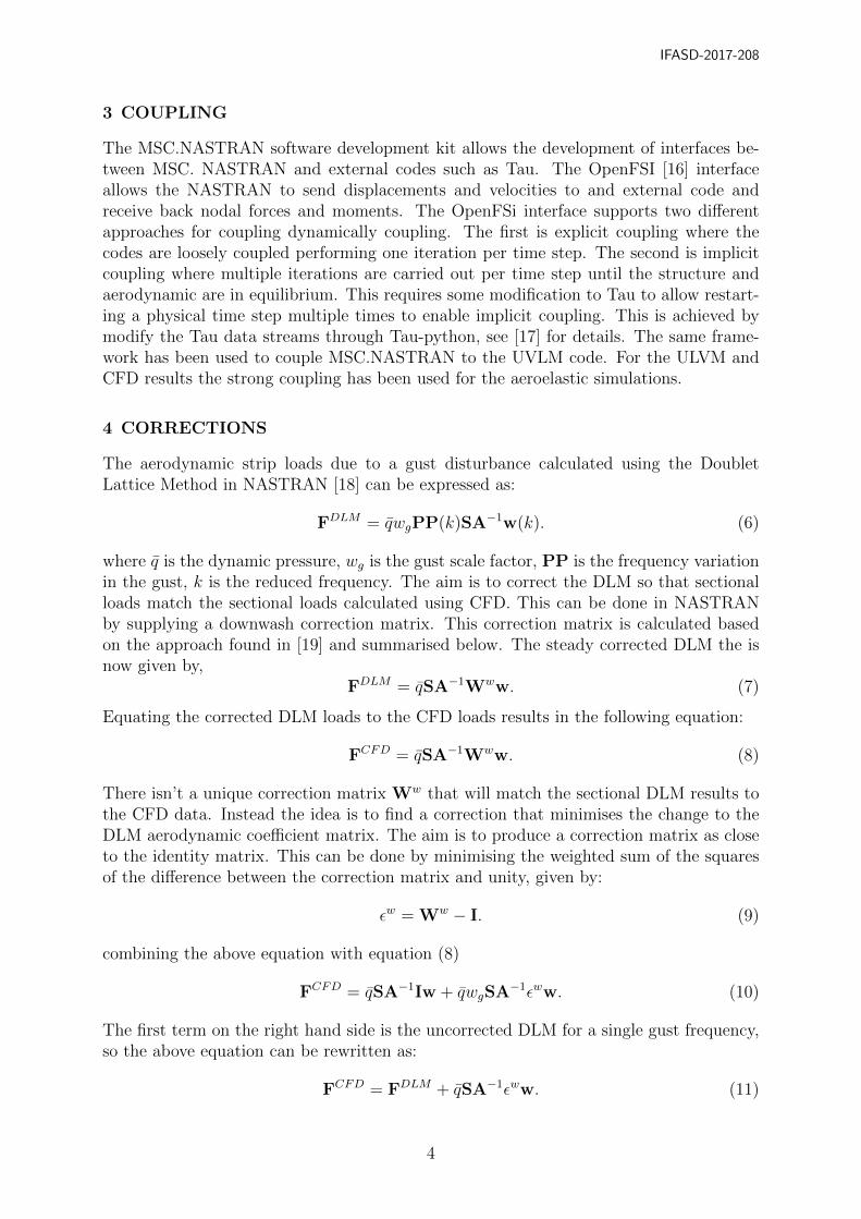
3 COUPLING

The MSC.NASTRAN software development kit allows the development of interfaces be-tween MSC. NASTRAN and external codes such as Tau. The OpenFSI [16] interfaceallows the NASTRAN to send displacements and velocities to and external code andreceive back nodal forces and moments. The OpenFSi interface supports two differentapproaches for coupling dynamically coupling. The first is explicit coupling where thecodes are loosely coupled performing one iteration per time step. The second is implicitcoupling where multiple iterations are carried out per time step until the structure andaerodynamic are in equilibrium. This requires some modification to Tau to allow restart-ing a physical time step multiple times to enable implicit coupling. This is achieved bymodify the Tau data streams through Tau-python, see [17] for details. The same frame-work has been used to couple MSC.NASTRAN to the UVLM code. For the ULVM andCFD results the strong coupling has been used for the aeroelastic simulations.

4 CORRECTIONS

The aerodynamic strip loads due to a gust disturbance calculated using the DoubletLattice Method in NASTRAN [18] can be expressed as:

FDLM = qwgPP(k)SA−1w(k). (6)

where q is the dynamic pressure, wg is the gust scale factor, PP is the frequency variationin the gust, k is the reduced frequency. The aim is to correct the DLM so that sectionalloads match the sectional loads calculated using CFD. This can be done in NASTRANby supplying a downwash correction matrix. This correction matrix is calculated basedon the approach found in [19] and summarised below. The steady corrected DLM the isnow given by,

FDLM = qSA−1Www. (7)

Equating the corrected DLM loads to the CFD loads results in the following equation:

FCFD = qSA−1Www. (8)

There isn’t a unique correction matrix Ww that will match the sectional DLM results tothe CFD data. Instead the idea is to find a correction that minimises the change to theDLM aerodynamic coefficient matrix. The aim is to produce a correction matrix as closeto the identity matrix. This can be done by minimising the weighted sum of the squaresof the difference between the correction matrix and unity, given by:

εw = Ww − I. (9)

combining the above equation with equation (8)

FCFD = qSA−1Iw + qwgSA−1εww. (10)

The first term on the right hand side is the uncorrected DLM for a single gust frequency,so the above equation can be rewritten as:

FCFD = FDLM + qSA−1εww. (11)

4

IFASD-2017-208

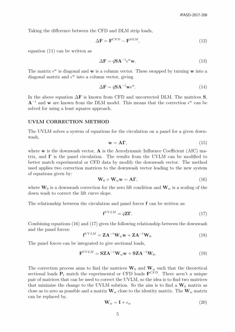
Taking the difference between the CFD and DLM strip loads,

∆F = FCFD − FDLM , (12)

equation (11) can be written as

∆F = qSA−1εww. (13)

The matrix εw is diagonal and w is a column vector. These swapped by turning w into adiagonal matrix and εw into a column vector, giving

∆F = qSA−1wεw. (14)

In the above equation ∆F is known from CFD and uncorrected DLM. The matrices S,A−1 and w are known from the DLM model. This means that the correction εw can besolved for using a least squares approach.

UVLM CORRECTION METHOD

The UVLM solves a system of equations for the circulation on a panel for a given down-wash,

w = AΓ, (15)

where w is the downwash vector, A is the Aerodynamic Influence Coefficient (AIC) ma-trix, and Γ is the panel circulation. The results from the UVLM can be modified tobetter match experimental or CFD data by modify the downwash vector. The methodused applies two correction matrices to the downwash vector leading to the new systemof equations given by:

W0 + Www = AΓ, (16)

where W0 is a downwash correction for the zero lift condition and Ww is a scaling of thedown wash to correct the lift curve slope.

The relationship between the circulation and panel forces f can be written as:

fUV LM = qZΓ. (17)

Combining equations (16) and (17) gives the following relationship between the downwashand the panel forces:

fUV LM = ZA−1Www + ZA−1W0. (18)

The panel forces can be integrated to give sectional loads,

FUV LM = SZA−1Www + SZA−1W0, (19)

The correction process aims to find the matrices W0 and Ww such that the theoreticalsectional loads Pt match the experimental or CFD loads FCFD. There aren’t a uniquepair of matrices that can be used to correct the UVLM, so the idea is to find two matricesthat minimise the change to the UVLM solution. So the aim is to find a W0 matrix asclose as to zero as possible and a matrix Ww close to the identity matrix. The Ww matrixcan be replaced by,

Ww = I + εw (20)

5

IFASD-2017-208

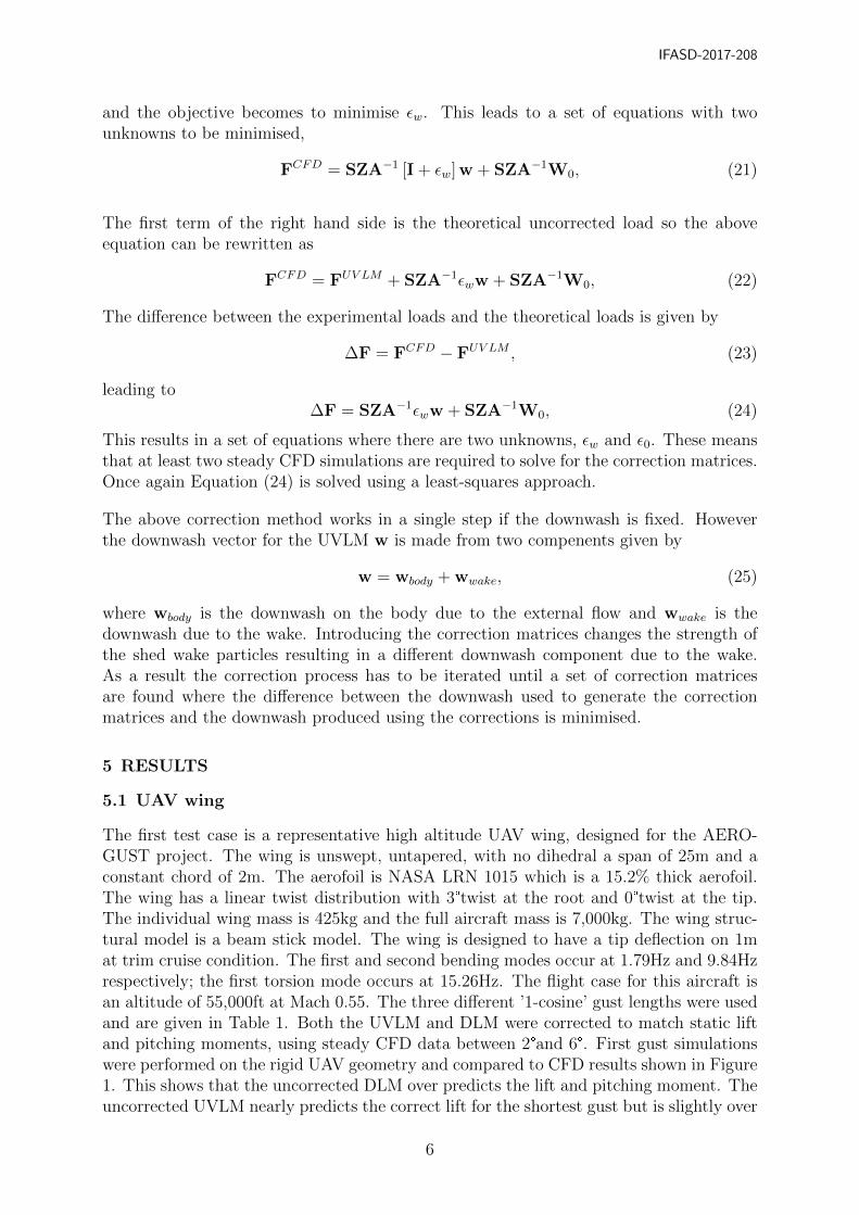
and the objective becomes to minimise εw. This leads to a set of equations with twounknowns to be minimised,

FCFD = SZA−1 [I + εw] w + SZA−1W0, (21)

The first term of the right hand side is the theoretical uncorrected load so the aboveequation can be rewritten as

FCFD = FUV LM + SZA−1εww + SZA−1W0, (22)

The difference between the experimental loads and the theoretical loads is given by

∆F = FCFD − FUV LM , (23)

leading to∆F = SZA−1εww + SZA−1W0, (24)

This results in a set of equations where there are two unknowns, εw and ε0. These meansthat at least two steady CFD simulations are required to solve for the correction matrices.Once again Equation (24) is solved using a least-squares approach.

The above correction method works in a single step if the downwash is fixed. Howeverthe downwash vector for the UVLM w is made from two compenents given by

w = wbody + wwake, (25)

where wbody is the downwash on the body due to the external flow and wwake is thedownwash due to the wake. Introducing the correction matrices changes the strength ofthe shed wake particles resulting in a different downwash component due to the wake.As a result the correction process has to be iterated until a set of correction matricesare found where the difference between the downwash used to generate the correctionmatrices and the downwash produced using the corrections is minimised.

5 RESULTS

5.1 UAV wing

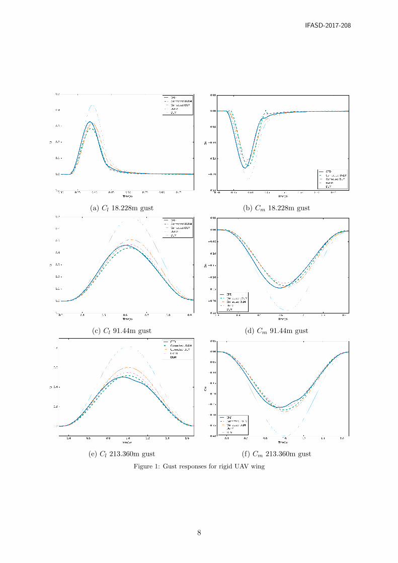
The first test case is a representative high altitude UAV wing, designed for the AERO-GUST project. The wing is unswept, untapered, with no dihedral a span of 25m and aconstant chord of 2m. The aerofoil is NASA LRN 1015 which is a 15.2% thick aerofoil.The wing has a linear twist distribution with 3°twist at the root and 0°twist at the tip.The individual wing mass is 425kg and the full aircraft mass is 7,000kg. The wing struc-tural model is a beam stick model. The wing is designed to have a tip deflection on 1mat trim cruise condition. The first and second bending modes occur at 1.79Hz and 9.84Hzrespectively; the first torsion mode occurs at 15.26Hz. The flight case for this aircraft isan altitude of 55,000ft at Mach 0.55. The three different ’1-cosine’ gust lengths were usedand are given in Table 1. Both the UVLM and DLM were corrected to match static liftand pitching moments, using steady CFD data between 2°and 6°. First gust simulationswere performed on the rigid UAV geometry and compared to CFD results shown in Figure1. This shows that the uncorrected DLM over predicts the lift and pitching moment. Theuncorrected UVLM nearly predicts the correct lift for the shortest gust but is slightly over

6

IFASD-2017-208

Gust length(m) Gust amplitude(m/s)18.288 11.70091.440 15.310213.360 17.634

Table 1: ’1-cosine’ gust parameters used for UAV wing

for the longer gust lengths. However the uncorrected UVLM over predicts the pitchingmoment slightly more the DLM. Applying the correction the DLM still over predicts thelift for the longer gusts, but is quite close for the shortest gust. The pitching momentsshows better agreement for the longer gusts although it now under predicts the shortestgust. The UVLM which was predicted the lift better now under predicts the lift for theshortest two gusts when the correction is applied. However the correction does improvethe UVLMs prediction of the pitching moment. In all cases the DLM and UVLM predictthe peak response slightly latter the the CFD.

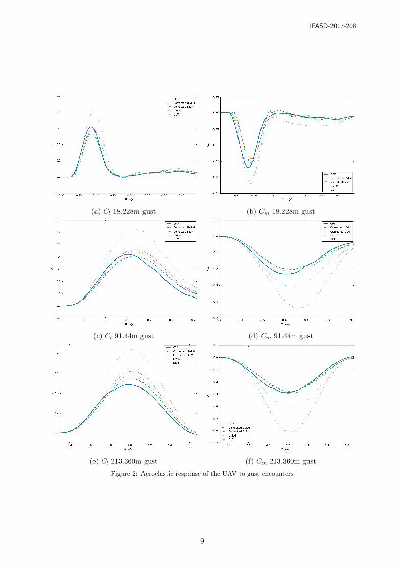
Next the corrections were applied to an aeroelastic simulation of the UAV wing encoun-tering a gust with the wing route fixed, shown in Figure 2. For both the UVLM and CFDresults the aircraft was trimmed to match the flight Cl and achieve a steady aeroelasticshape to start the gust simulations from. The results for the aeroelastic case show similartrends to the rigid case. For the lift the corrected DLM produces better results for theshortest gust while the corrected UVLM is closer for the longer two gusts. Both correctedapproaches under predict the moment for the shortest two gusts but are both fairly closefor the longest gust. Once again the peak loads are predicted slightly later.

5.2 NCRM

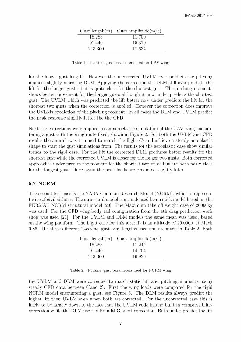
The second test case is the NASA Common Research Model (NCRM), which is represen-tative of civil airliner. The structural model is a condensed beam stick model based on theFERMAT NCRM structural model [20]. The Maximum take off weight case of 26000kgwas used. For the CFD wing body tail configuration from the 4th drag prediction workshop was used [21]. For the UVLM and DLM models the same mesh was used, basedon the wing planform. The flight case for this aircraft is an altitude of 29,000ft at Mach0.86. The three different ’1-cosine’ gust were lengths used and are given in Table 2. Both

Gust length(m) Gust amplitude(m/s)18.288 11.24491.440 14.704213.360 16.936

Table 2: ’1-cosine’ gust parameters used for NCRM wing

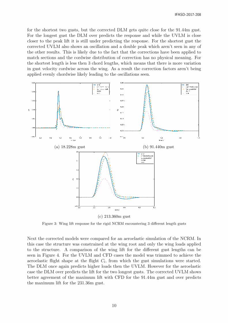
the UVLM and DLM were corrected to match static lift and pitching moments, usingsteady CFD data between 0°and 2°. First the wing loads were compared for the rigidNCRM model encountering a gust, see Figure 3. The DLM results always predict thehigher lift then UVLM even when both are corrected. For the uncorrected case this islikely to be largely down to the fact that the UVLM code has no built in compressibilitycorrection while the DLM use the Prandtl Glauert correction. Both under predict the lift

7

IFASD-2017-208

(a) Cl 18.228m gust (b) Cm 18.228m gust

(c) Cl 91.44m gust (d) Cm 91.44m gust

(e) Cl 213.360m gust (f) Cm 213.360m gust

Figure 1: Gust responses for rigid UAV wing

8

IFASD-2017-208

(a) Cl 18.228m gust (b) Cm 18.228m gust

(c) Cl 91.44m gust (d) Cm 91.44m gust

(e) Cl 213.360m gust (f) Cm 213.360m gust

Figure 2: Aeroelastic response of the UAV to gust encounters

9

IFASD-2017-208

for the shortest two gusts, but the corrected DLM gets quite close for the 91.44m gust.For the longest gust the DLM over predicts the response and while the UVLM is closecloser to the peak lift it is still under predicting the response. For the shortest gust thecorrected UVLM also shows an oscillation and a double peak which aren’t seen in any ofthe other results. This is likely due to the fact that the corrections have been applied tomatch sections and the cordwise distribution of correction has no physical meaning. Forthe shortest length is less then 3 chord lengths, which means that there is more variationin gust velocity cordwise across the wing. As a result the correction factors aren’t beingapplied evenly chordwise likely leading to the oscillations seen.

(a) 18.228m gust (b) 91.440m gust

(c) 213.360m gust

Figure 3: Wing lift response for the rigid NCRM encountering 3 different length gusts

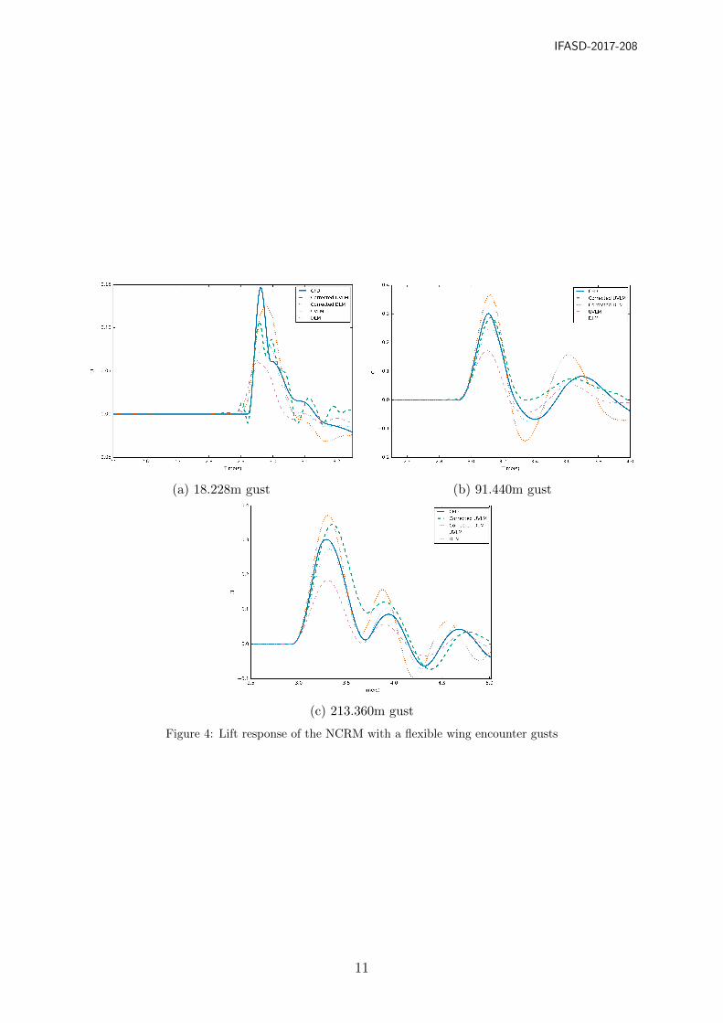
Next the corrected models were compared for an aeroelastic simulation of the NCRM. Inthis case the structure was constrained at the wing root and only the wing loads appliedto the structure. A comparison of the wing lift for the different gust lengths can beseen in Figure 4. For the UVLM and CFD cases the model was trimmed to achieve theaeroelastic flight shape at the flight Cl, from which the gust simulations were started.The DLM once again predicts higher loads then the UVLM. However for the aeroelasticcase the DLM over predicts the lift for the two longest gusts. The corrected UVLM showsbetter agreement of the maximum lift with CFD for the 91.44m gust and over predictsthe maximum lift for the 231.36m gust.

10

IFASD-2017-208

(a) 18.228m gust (b) 91.440m gust

(c) 213.360m gust

Figure 4: Lift response of the NCRM with a flexible wing encounter gusts

11

IFASD-2017-208

6 CONCLUSIONS

A method for correcting the UVLM based on a downwash correction has been comparedto the equivalent approach for the DLM. The two approaches haven compare for twoconfigurations encountering three different length ”1-cosine” gusts representative of theseprescribed in the CS-25 requirements. For the cases investigated the correct DLM methodpredicts higher loads then the corrected UVLM method. Generally the DLM matches theshortest gust well and over predicts the longer gusts. While the corrected UVLM underpredicts the shortest gust be improves as the gust lengths increase.

ACKNOWLEDGMENTS

The research leading to these results has received funding from the AEROGUST project(funded by the European Commission under grant agreement number 636053). The part-ners in AEROGUST are: University of Bristol, INRIA, NLR, DLR, University of CapeTown, NUMECA, Optimad Engineering S.r.l., University of Liverpool, Airbus Defenseand Space, Dassault Aviation, Piaggio Aerospace and Valeol.

This work was carried out using the computational facilities of the Advanced ComputingResearch Centre, University of Bristol - http://www.bris.ac.uk/acrc/.

7 REFERENCES

[1] Baker, M. L. (1998). CFD based corrections for linear aerodynamic methods. AGARDReport, 822.

[2] Palacios, R., Climent, H., Karlsson, A., et al. (2001). Assessment of strategies forcorrecting linear unsteady aerodynamics using cfd or experimental results. In Pro-ceedings of the CEAS/AIAA International Forum on Aeroelasticity and StructuralDynamics. Confederation of European Aerospace Societies.

[3] Silva, R. G. A., Mello, O. A. F., Azevedo, J. L. F., et al. (2008). Investigation ontransonic correction methods for unsteady aerodynamics and aeroelastic analyses.Journal of Aircraft, 45(6), 1890–1903.

[4] Dimitrov, D. and Thormann, R. (2013). DLM-correction method for aerodynamicgust response prediction. In In IFASD 2013 16th International Forum on Aeroelas-ticity and Structural Dynamics, IFASD 2013-24.

[5] Valente, C., Lemmens, Y., Wales, C., et al. (2017). A doublet-lattice method correc-tion approach for high fidelity gust loads analysis. In 58th AIAA/ASCE/AHS/ASCStructures, Structural Dynamics, and Materials Conference, AIAA 2017-0632. Amer-ican Institute of Aeronautics and Astronautics Inc, AIAA. doi:10.2514/6.2017-0632.

[6] Albano, E. (1968). A doublet lattice method for calculating lift distributions onoscillating surfaces in subsonic flows. In 6th Aerospace Sciences Meeting, AIAA 1968-73. American Institute of Aeronautics and Astronautics. doi:10.2514/6.1968-73.

[7] Katz, J. and Plotkin, A. (2001). Low-speed aerodynamics. Cambridge universitypress.

12

IFASD-2017-208

[8] Greengard, L. and Rokhlin, V. (1987). A fast algorithm for particle simulations.Journal of computational physics, 73(2), 325–348.

[9] Losasso, F., Gibou, F., and Fedkiw, R. (2004). Simulating water and smoke with anoctree data structure. In ACM Transactions on Graphics (TOG), vol. 23. ACM, pp.457–462.

[10] Selle, A., Rasmussen, N., and Fedkiw, R. (2005). A vortex particle method for smoke,water and explosions. In ACM Transactions on Graphics (TOG), vol. 24. ACM, pp.910–914.

[11] Wales, C., Jones, D., and Gaitonde, A. (2015). Prescribed velocity method for sim-ulation of aerofoil gust responses. Journal of Aircraft, 52, 64–76. ISSN 0021-8869.doi:10.2514/1.C032597.

[12] Huntley, S., Jones, D., and Gaitonde, A. (2016). 2d and 3d gust response using aprescribed velocity method in viscous flows. In 46th AIAA Fluid Dynamics Con-ference, AIAA 2016-4259. American Institute of Aeronautics and Astronautics Inc,AIAA. ISBN 9781624104367. doi:10.2514/6.2016-4259.

[13] Gerhold, T., Friedrich, O., Evans, J., et al. (1997). Calculation of complex three-dimensional configurations employing the DLR-TAU-code. (AIAA 1997-0167).

[14] Galle, M., Gerhold, T., and Evans, J. (1999). Parallel computation of turbulent flowsaround complex geometries on hybrid grids with the DLR-TAU code. In A. Ecer andD. R. Emerson (Eds.), Proc. 11th Parallel CFD Conference.

[15] Allmaras, S. R. and Johnson, F. T. (2012). Modifications and clarifications for theimplementation of the spalart-allmaras turbulence model. In Seventh InternationalConference on Computational Fluid Dynamics (ICCFD7). pp. 1–11.

[16] MSC (2014). MSC Software Development Kit.

[17] Valente, C., Jones, D., Gaitonde, A., et al. (2015). Openfsi interface for stronglycoupled steady and unsteady aeroelasticity. In International Forum on Aeroelasticityand Structural Dynamics, IFASD 2015, IFASD 2013-178. International Forum onAeroelasticity and Structural Dynamics (IFASD).

[18] MSC (2014). Aeroelastic Analysis User’s Guide.

[19] Giesing, J., Kalman, T., and Rodden, W. P. (1976). Correction factory techniquesfor improving aerodynamic prediction methods. NASA CR-144967.

[20] Klimmek, T. (2013). Development of a structural model of the crm configurationfor aeroelastic and loads analysis. In In IFASD 2013 16th International Forum onAeroelasticity and Structural Dynamics, IFASD 2013-10.

[21] Vassberg, J., Dehaan, M., Rivers, M., et al. (2008). Development of a commonresearch model for applied cfd validation studies. In 26th AIAA Applied AerodynamicsConference, AIAA 2008-6919.

13

IFASD-2017-208

COPYRIGHT STATEMENT

The authors confirm that they, and/or their company or organization, hold copyright onall of the original material included in this paper. The authors also confirm that theyhave obtained permission, from the copyright holder of any third party material includedin this paper, to publish it as part of their paper. The authors confirm that they givepermission, or have obtained permission from the copyright holder of this paper, for thepublication and distribution of this paper as part of the IFASD-2017 proceedings or asindividual off-prints from the proceedings.

14