vol pore pressure prediction
TRANSCRIPT
CHEVRON DRILLING REFERENCE SERIESVOLUME FOUR
PORE PRESSURE PREDICTION
Page A - 1 Rev. 4/24/90
SECTION A: INTRODUCTION TO MODELING
1. INTRODUCTION
Probing the earth’s subsurface for oil and gas presents many challenges and surprises.Developing an understanding of this subsurface and attempting to predict, withreasonable success, what lies ahead is a major significant factor in drilling safely, drillingeconomically and drilling useable, productive wells. At the core of this understandingshould lie a strong fundamental knowledge of pore pressure, it’s development, anomaliesassociated with normal, abnormal, and subnormal pore pressure and predictivetechniques which can be used as well planning and real time drilling tools.
Certainly, it is true that not all wells drilled world-wide are planned or programmed basedupon pore pressure predictions. However, this does not eliminate the need forknowledge in this area since drilling environments are constantly changing and, eventhough abnormal pressure may not be present, normal or subnormal pressures may be.Prediction, evaluation and reaction to these environments is necessary (Figure 4A.1).
This introduction presents current technology, equations, and some examples of porepressure prediction techniques. It should be kept in mind that the material presentedhere does have its limitations, but when consistently and carefully applied, it is a veryuseful tool, from both a well planning standpoint and a “real time” drilling standpoint.
Two key points are worth mentioning at this time. First, the accuracy of these techniquesand the usefulness of the results are directly proportional to the amount of historical andoffset information used. Secondly, as drilling engineers, a great deal of our success andwell planners will stem from our ability to communicate with local exploration staffs andobtain as much information as possible. As drilling engineers, we must be aware of the
Figure 4A.1
WHY?
• • Predict Abnormal Pressure • • Drill Fast • • Drill Safe
CHEVRON DRILLING REFERENCE SERIESVOLUME FOURPORE PRESSURE PREDICTION
Page A - 2 Rev. 4/24/90
data and information needed and be able to communicate this to the explorationgeologist.
2. SEDIMENTATION
Thousands of feet of sediment have been deposited over millions of years. It started assoon as the earth had cooled enough to allow rainfall and has continued until today.Historical geology is a fascinating study and makes excellent reading for any drillingengineer.
Consider the drainage area of the Mississippi River. From Jackson Hole, Wyoming,comes pieces of stone that are deposited south of New Orleans as sand. From Ely,Minnesota, comes pine needles, leaves and more sand, and, further down the river, silt,grass and other organic material. Reason suggests that more silt comes down the rivernow than did when the drainage area was covered by grass and trees.
As this material reaches the Gulf, the sand settles out first near the shore. In deeperwater, only mud, silt, and organic material reach the ocean floor. The depth of abnormalpressure can be a function of distance from a major river during the depositional phase.
3. COMPACTION
Consider one cubic foot of sediment just settled to the ocean floor in the Gulf of Mexico.Just deposited, it would be hard to tell mud from water, but as it rests on bottom, thesolid material would settle to bottom and the water would flow away. Finally, one cubicfoot of mud is left (Figure 4A.2).

CHEVRON DRILLING REFERENCE SERIESVOLUME FOUR
PORE PRESSURE PREDICTION
Page A - 3 Rev. 4/24/90
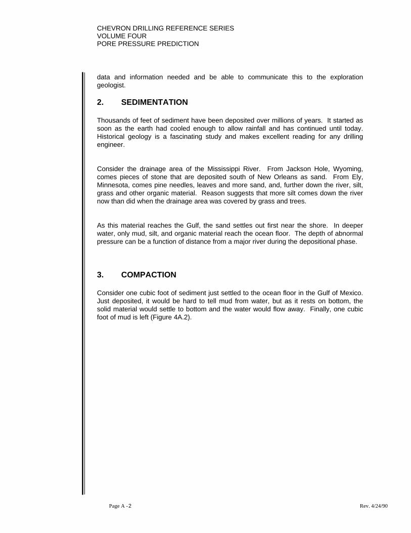
To assist in the analysis of this condition, consider the soil boring analysis in figures 4A.3and 4A.4. Examine sample #1. It is interesting to note that its density was 89 lb/ft3, or11.9 ppg. This is certainly not yet shale.

CHEVRON DRILLING REFERENCE SERIESVOLUME FOURPORE PRESSURE PREDICTION
Page A - 4 Rev. 4/24/90
CHEVRON DRILLING REFERENCE SERIESVOLUME FOUR
PORE PRESSURE PREDICTION
Page A - 5 Rev. 4/24/90
We believe the specific gravity of normally-compacted shale to be about 2.6 (21.7 ppg).Although we do not have shale yet (sample #1), we might assume that the grain densityof the sediments is 19.0 ppg. Also, assume that the density of the sea water is 9.0 ppg.
CHEVRON DRILLING REFERENCE SERIESVOLUME FOURPORE PRESSURE PREDICTION
Page A - 6 Rev. 4/24/90
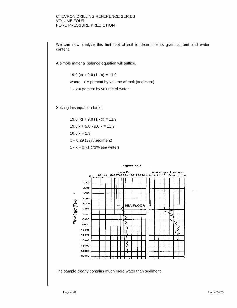
We can now analyze this first foot of soil to determine its grain content and watercontent.
A simple material balance equation will suffice.
19.0 (x) + 9.0 (1 - x) = 11.9
where: x = percent by volume of rock (sediment)
1 - x = percent by volume of water
Solving this equation for x:
19.0 (x) + 9.0 (1 - x) = 11.9
19.0 x + 9.0 - 9.0 x = 11.9
10.0 x = 2.9
x = 0.29 (29% sediment)
1 - x = 0.71 (71% sea water)
The sample clearly contains much more water than sediment.

CHEVRON DRILLING REFERENCE SERIESVOLUME FOUR
PORE PRESSURE PREDICTION
Page A - 7 Rev. 4/24/90
The interesting thing about compaction is that each cubic foot of mud below this has noway of getting rid of its water with the exception that it leak through the cubic foot we areconsidering. So, as this cubic foot compacts under weight, it gives off water but receivesmore water from below. Thus, compaction is a very lengthy process.
This newly deposited cubic foot of mud also contains organic material that will give offmethane gas, further aggravating the process of compaction, and certainly complicatingthe drilling process.
To illustrate this point further, consider the last data point on the referenced report. Notethat at a penetration depth of 698 feet, the density was 122 lb/ft3 or 16.3 ppg.Proceeding with a similar analysis, we find the following:
19.0 (x) + 9.0 (1 - x) = 16.3
19.0 x + 9.0 - 9.0 x = 16.3
10.0 x = 7.3
x = 0.73 (73% sediment)
1 - x = 0.27 (27% sea water)
This analysis indicates that even at 698 feet, grain-to-grain contact has not yet beenestablished and we certainly do not yet have shale. It is worth noting that in many youngsedimentary basins, this grain-to-grain contact is not established until a depth of possibly3000 - 5000 feet, as shown in Figure 4A.6.

CHEVRON DRILLING REFERENCE SERIESVOLUME FOURPORE PRESSURE PREDICTION
Page A - 8 Rev. 4/24/90
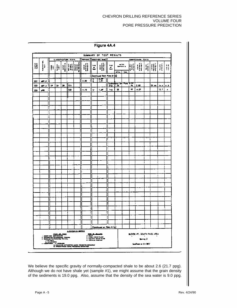
One final observation concerning this soil boring report is worth noting. Consider the plotof density versus depth on semi-logarithmic scale as shown in Figure 4A.5. The first 250- 270 feet below the sea floor seems to be compacting at a different rate than thosesediments below. Actually, the top sediments are moving and very unstable. This, ofcourse, contributes to a very difficult drilling environment.
Important points to remember are listed in Figure 4A.7.
4. NORMAL PRESSURE
The process by which mud is changed into a solid as sedimentation occurs is calledcompaction. Generally in the Gulf of Mexico the sediments do not achieve grain-to-grain
Figure 4A.7
Compaction
• • Compaction is a very lengthy process. • • Water must escape in order for grain-to-grain contact to be
established. • • Near the surface, sediments act partially like rock and partially
like mud. • • The earth's density is variable with depth. (In young
sedimentary basins) • • The earth's density will not plot as a straight line on semi-
logarithmic paper until grain-to-grain contact is established.This may not occur until a depth of 3000 5000 feet has beenreached.

CHEVRON DRILLING REFERENCE SERIESVOLUME FOUR
PORE PRESSURE PREDICTION
Page A - 9 Rev. 4/24/90
contact until a depth of 3,000 - 5,000 feet has been achieved. Typically in hard rockenvironments, like West Texas, the unconsolidated interval may only be 100 - 200 feet,obviously a much different environment. The fundamental point however, is that whengrain-to-grain contact has been established, and the water in the rock is free to move,normal pore pressure exists.
This normal pressure is dependent on two parameters: 1) Pore fluid density, and 2)Vertical fluid column height, as shown in Figure 4A.8. For most young sedimentarydrilling environments, the fluid density in the rock pore spaces will be about 9 ppg, orexhibit a pressure gradient of .468 psi/ft. This is somewhat different in older hard rockenvironments where the formation waters may be less saline (lower density) and thewater table may be lower. It is not uncommon to find effective fluid densities at depth tobe as low as 8.25 ppg (.429 psi/ft). Note that this is "effective” density and indeed can beless than fresh water. To summarize, normal formation pressure is simply thehydrostatic pressure exerted by a continuous fluid column at some depth, as in Figure4A.9. It is dependent on fluid density and the vertical column height of the fluid.
Another way to visualize normal formation pressure is to examine a plot of formationdensity on a logarithmic scale versus depth on a linear scale (see Figure 4A.6). It is

CHEVRON DRILLING REFERENCE SERIESVOLUME FOURPORE PRESSURE PREDICTION
Page A - 10 Rev. 4/24/90
common to find that a straight line can be drawn through formation density only aftergrain-to-grain contact has been established and covering only those sediments which arenormally pressured. Therefore, it could be said that normal pressure exists whenformation density increases with depth in such a way that a straight line can be drawnthrough the plotted points on semi-log paper. This straight line is called the "normal trendline" and the slope of the line is an indicator of the rate at which the shale hascompacted.
To summarize, the key points about normally pressured sediments are (Figure 4A.10):
CHEVRON DRILLING REFERENCE SERIESVOLUME FOUR
PORE PRESSURE PREDICTION
Page A - 11 Rev. 4/24/90
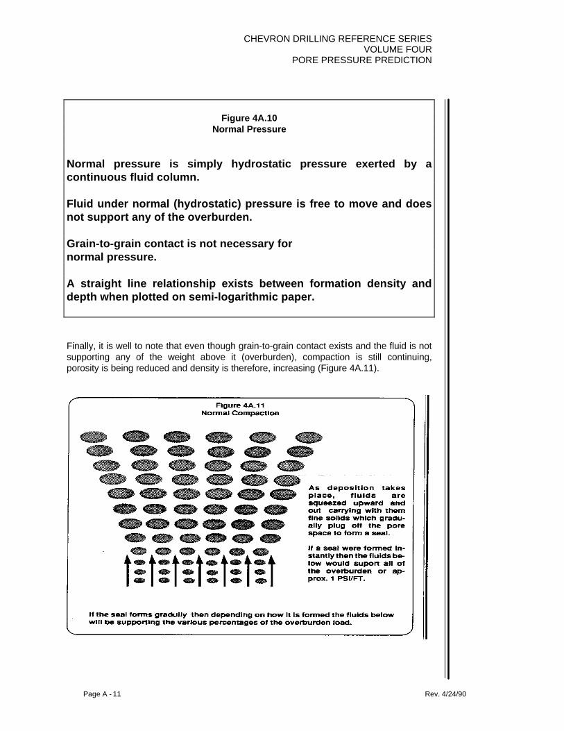
Finally, it is well to note that even though grain-to-grain contact exists and the fluid is notsupporting any of the weight above it (overburden), compaction is still continuing,porosity is being reduced and density is therefore, increasing (Figure 4A.11).
Figure 4A.10Normal Pressure
Normal pressure is simply hydrostatic pressure exerted by acontinuous fluid column.
Fluid under normal (hydrostatic) pressure is free to move and doesnot support any of the overburden.
Grain-to-grain contact is not necessary fornormal pressure.
A straight line relationship exists between formation density anddepth when plotted on semi-logarithmic paper.
CHEVRON DRILLING REFERENCE SERIESVOLUME FOURPORE PRESSURE PREDICTION
Page A - 12 Rev. 4/24/90
5. ABNORMAL PRESSURE
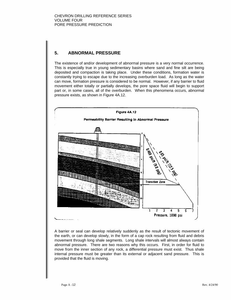
The existence of and/or development of abnormal pressure is a very normal occurrence.This is especially true in young sedimentary basins where sand and fine silt are beingdeposited and compaction is taking place. Under these conditions, formation water isconstantly trying to escape due to the increasing overburden load. As long as the watercan move, formation pressure is considered to be normal. However, if any barrier to fluidmovement either totally or partially develops, the pore space fluid will begin to supportpart or, in some cases, all of the overburden. When this phenomena occurs, abnormalpressure exists, as shown in Figure 4A.12.
A barrier or seal can develop relatively suddenly as the result of tectonic movement ofthe earth, or can develop slowly, in the form of a cap rock resulting from fluid and debrismovement through long shale segments. Long shale intervals will almost always containabnormal pressure. There are two reasons why this occurs. First, in order for fluid tomove from the inner section of any rock, a differential pressure must exist. Thus shaleinternal pressure must be greater than its external or adjacent sand pressure. This isprovided that the fluid is moving.
CHEVRON DRILLING REFERENCE SERIESVOLUME FOUR
PORE PRESSURE PREDICTION
Page A - 13 Rev. 4/24/90
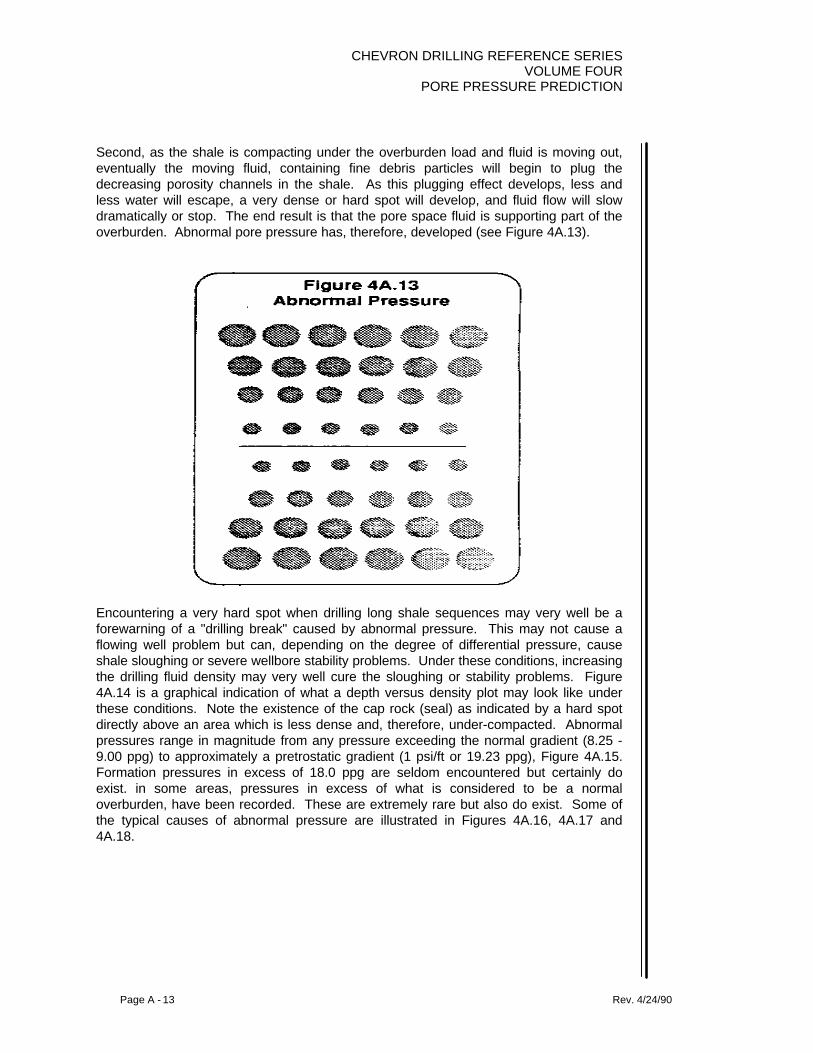
Second, as the shale is compacting under the overburden load and fluid is moving out,eventually the moving fluid, containing fine debris particles will begin to plug thedecreasing porosity channels in the shale. As this plugging effect develops, less andless water will escape, a very dense or hard spot will develop, and fluid flow will slowdramatically or stop. The end result is that the pore space fluid is supporting part of theoverburden. Abnormal pore pressure has, therefore, developed (see Figure 4A.13).
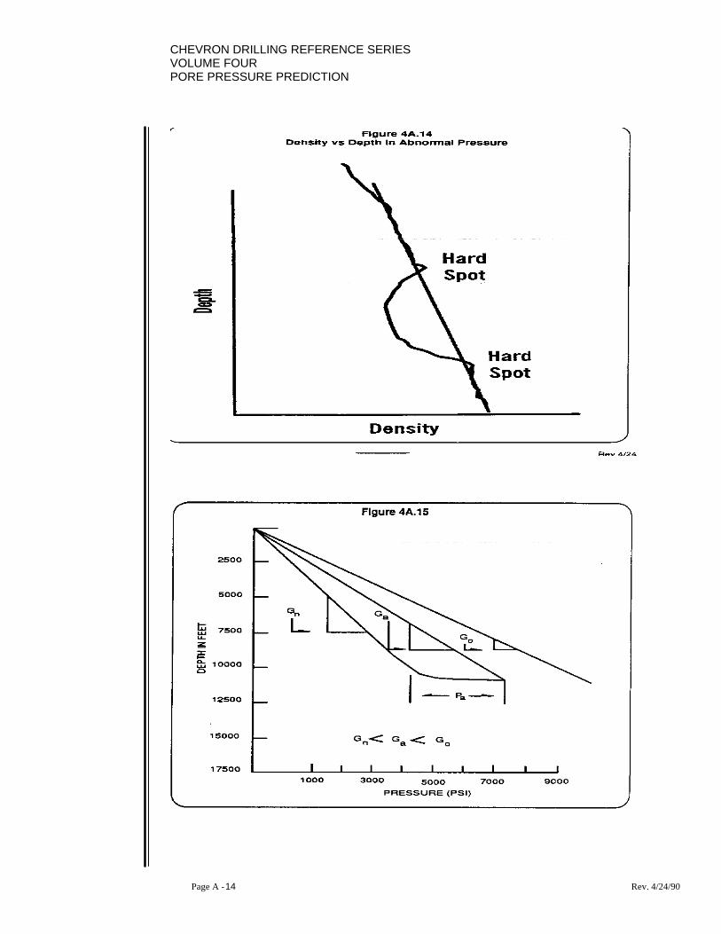
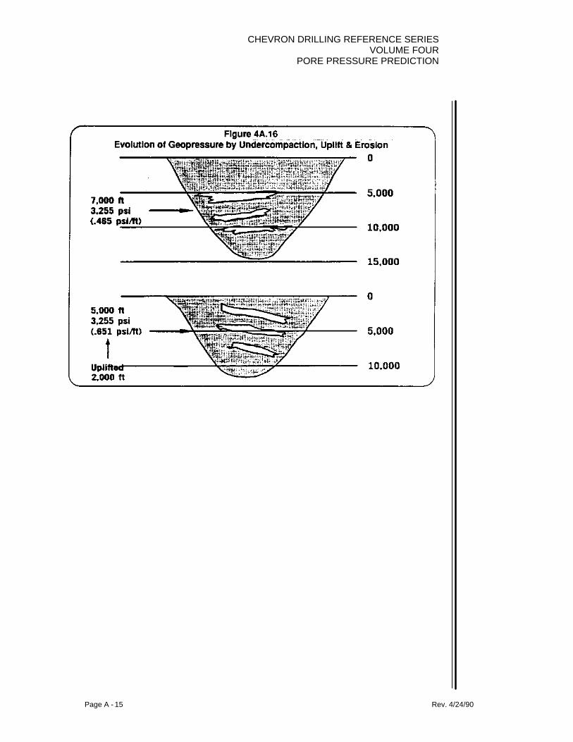
Encountering a very hard spot when drilling long shale sequences may very well be aforewarning of a "drilling break" caused by abnormal pressure. This may not cause aflowing well problem but can, depending on the degree of differential pressure, causeshale sloughing or severe wellbore stability problems. Under these conditions, increasingthe drilling fluid density may very well cure the sloughing or stability problems. Figure4A.14 is a graphical indication of what a depth versus density plot may look like underthese conditions. Note the existence of the cap rock (seal) as indicated by a hard spotdirectly above an area which is less dense and, therefore, under-compacted. Abnormalpressures range in magnitude from any pressure exceeding the normal gradient (8.25 -9.00 ppg) to approximately a pretrostatic gradient (1 psi/ft or 19.23 ppg), Figure 4A.15.Formation pressures in excess of 18.0 ppg are seldom encountered but certainly doexist. in some areas, pressures in excess of what is considered to be a normaloverburden, have been recorded. These are extremely rare but also do exist. Some ofthe typical causes of abnormal pressure are illustrated in Figures 4A.16, 4A.17 and4A.18.
CHEVRON DRILLING REFERENCE SERIESVOLUME FOURPORE PRESSURE PREDICTION
Page A - 14 Rev. 4/24/90
CHEVRON DRILLING REFERENCE SERIESVOLUME FOUR
PORE PRESSURE PREDICTION
Page A - 15 Rev. 4/24/90

CHEVRON DRILLING REFERENCE SERIESVOLUME FOURPORE PRESSURE PREDICTION
Page A - 16 Rev. 4/24/90

CHEVRON DRILLING REFERENCE SERIESVOLUME FOUR
PORE PRESSURE PREDICTION
Page A - 17 Rev. 4/24/90
6. ABNORMAL PRESSURE INDICATORS
Years ago the main indicator of abnormal pressure was a kick or even a blowout.Increasing the drilling fluid density seemed to be the answer to prevent thesecatastrophes. It was soon discovered, however, that by indiscriminately increasing thefluid density other problems arose. Namely, lost circulation, stuck pipe, and evenadditional wellbore kicks and blowouts. Obviously, it is most desirable to drill with thefluid density as close as possible to the formation pressure. Above all, we must drillsafely, but at the same time, drill efficiently with minimum wellbore and fluid problems.
Two related concepts had to be developed in order that this might be accomplished.First, the ability to predict formation pressures had to be developed and secondly,methods or indicators of abnormal pressure while drilling had to be recognized andunderstood.
There are three stages in pore pressure determination 1) Before, 2) During, and 3) After(Figure 4A.19).
Before refers to prediction. We willfirst discuss several methods forpredicting the existence andmagnitude of abnormal pressures. Inrelatively young sedimentary basins,shale property trends can be usedvery effectively to illustrate how rockdensity varies with depth andtherefore, can also be used to predictpore pressures.
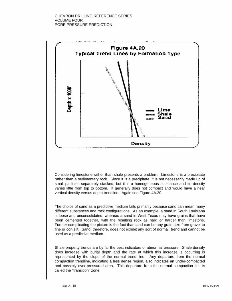
The reasons why shale trends are used are straight forward but certainly worthy ofmentioning. Generally, shale is composed of fine organic and mineral substances ofmore or less uniform particle size. But more importantly, shale compacts uniformly andpredictably. Thus, shale sequences do have a “normal” trend line illustrating an increaseintensity with depth, as depicted in Figure 4A.20.
Figure 4A.19
Stages of Detection
• • Before
• • During
• • After
CHEVRON DRILLING REFERENCE SERIESVOLUME FOURPORE PRESSURE PREDICTION
Page A - 18 Rev. 4/24/90
Considering limestone rather than shale presents a problem. Limestone is a precipitaterather than a sedimentary rock. Since it is a precipitate, it is not necessarily made up ofsmall particles separately stacked, but it is a homogeneous substance and its densityvaries little from top to bottom. It generally does not compact and would have a nearvertical density versus depth trendline. Again see Figure 4A.20.
The choice of sand as a predictive medium fails primarily because sand can mean manydifferent substances and rock configurations. As an example, a sand in South Louisianais loose and unconsolidated, whereas a sand in West Texas may have grains that havebeen cemented together, with the resulting rock as hard or harder than limestone.Further complicating the picture is the fact that sand can be any grain size from gravel tofine silicon silt. Sand, therefore, does not exhibit any sort of normal trend and cannot beused as a predictive medium.
Shale property trends are by far the best indicators of abnormal pressure. Shale densitydoes increase with burial depth and the rate at which this increase is occurring isrepresented by the slope of the normal trend line. Any departure from the normalcompaction trendline, indicating a less dense region, also indicates an under-compactedand possibly over-pressured area. This departure from the normal compaction line iscalled the “transition" zone.
CHEVRON DRILLING REFERENCE SERIESVOLUME FOUR
PORE PRESSURE PREDICTION
Page A - 19 Rev. 4/24/90
From a well planning standpoint, it seems logical that, after developing a soundsubsurface correlation between a new well to be drilled and previously drilled wells, anyand all data should be used to develop shale property trends so as to indicate wheretransition zones can be anticipated and what the magnitude of the abnormal pressuremight be. This data can also be used to calculate an anticipated fracture gradient. Thisis a very important element in the well planning and drilling process and will be discussedlater.
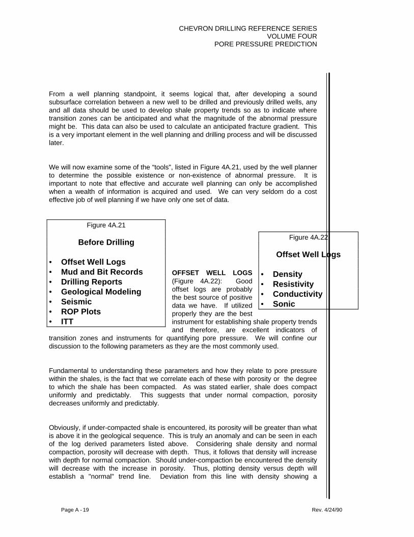
We will now examine some of the “tools", listed in Figure 4A.21, used by the well plannerto determine the possible existence or non-existence of abnormal pressure. It isimportant to note that effective and accurate well planning can only be accomplishedwhen a wealth of information is acquired and used. We can very seldom do a costeffective job of well planning if we have only one set of data.
OFFSET WELL LOGS(Figure 4A.22): Goodoffset logs are probablythe best source of positivedata we have. If utilizedproperly they are the bestinstrument for establishing shale property trendsand therefore, are excellent indicators of
transition zones and instruments for quantifying pore pressure. We will confine ourdiscussion to the following parameters as they are the most commonly used.
Fundamental to understanding these parameters and how they relate to pore pressurewithin the shales, is the fact that we correlate each of these with porosity or the degreeto which the shale has been compacted. As was stated earlier, shale does compactuniformly and predictably. This suggests that under normal compaction, porositydecreases uniformly and predictably.
Obviously, if under-compacted shale is encountered, its porosity will be greater than whatis above it in the geological sequence. This is truly an anomaly and can be seen in eachof the log derived parameters listed above. Considering shale density and normalcompaction, porosity will decrease with depth. Thus, it follows that density will increasewith depth for normal compaction. Should under-compaction be encountered the densitywill decrease with the increase in porosity. Thus, plotting density versus depth willestablish a "normal" trend line. Deviation from this line with density showing a
Figure 4A.21
Before Drilling
• • Offset Well Logs• • Mud and Bit Records• • Drilling Reports• • Geological Modeling• • Seismic• • ROP Plots• • ITT
Figure 4A.22
Offset Well Logs
• • Density• • Resistivity• • Conductivity• • Sonic
CHEVRON DRILLING REFERENCE SERIESVOLUME FOURPORE PRESSURE PREDICTION
Page A - 20 Rev. 4/24/90
decreasing trend will indicate under-compaction and possibly abnormal pressure. SeeFigure 4A.6 for an example plot.
Second, consider the effects on shale resistivity. For normal compaction, with porositydecreasing and density increasing, shale resistivity will be increasing. Understand thatas compaction is taking place, water is being forced up and out of these sediments.Water is the conductive medium, therefore, conductivity must be declining and resistivitymust be increasing. The opposite trend occurs when drilling a transition zone. Whenunder-compaction is present, porosity has increased, density has decreased, andresistivity has, therefore, decreased.
Again, this is due to the presence of more water, therefore, a more conductive, lessresistive rock. By considering resistivity, we have in fact also considered conductivity.Without too much redundancy, it is sufficient to say that under normal compaction, wateris being driven out, therefore, conductivity must be decreasing. Upon entering an under-compacted region with an increased porosity and water content, the conductivity will beincreased.
Finally, the sonic log must be considered. The sonic log actually indicates the intervaltransit time (T), of a sound wave traveling through the formation and back to a receiver.The units indicated on the sonic log are micro-seconds per foot (∆sec/ft). Note that sonicvelocity (feet/sec) is simply the reciprocal of the interval transit time multiplied by 106 (Vel= 106 / T).
Sonic log analysis for pore pressure prediction is developed around the concept that asporosity decreases and density increases, for normal compaction with depth, the rockbecomes a much more efficient sonic conductor. The sonic velocity will increase withdepth for normal compaction. Thus travel time (T) will decrease with depth, ifcompaction is uniform and considered normal. It follows that, when under-compactionexists, the sonic velocity will decrease thereby indicating an increasing interval transittime.
A graphical interpretation of each of the above properties is illustrated in Figure 4A.23.

CHEVRON DRILLING REFERENCE SERIESVOLUME FOUR
PORE PRESSURE PREDICTION
Page A - 21 Rev. 4/24/90
One final parameter which should be mentioned here is temperature. The earth's core isobviously hotter than its surface, therefore,. heat moves from the center to the surface.This phenomena creates a temperature gradient which is generally between 1°F and2°F per 100 ft. The earth's sediments are actually functioning as a heat exchanger andthe flow rate of heat through any formation is directly proportional to the formationdensity. The higher the formation density, the smaller the temperature drop required togenerate a given heat flow.
Since abnormally pressured sediments are generally less dense than the normallypressured sediments above, there is generally a measurable increase in flow linetemperature if abnormal pressure is encountered. A plot of differential temperature per100 ft versus depth will be a straight line through normally pressured sediments. Theslope of that line will be in the range 1°F to 2°F per 100 ft. Upon drilling abnormallypressured sediments (less dense formations) the plot of differential temperature per 100ft. will show an increasing slope which is indicative of the earth functioning as a lessefficient heat exchanger.
More temperature drop is require to maintain a given heat flow rate. A plot of this typewould look very similar to an interval transit time versus depth plot, or would correlate

CHEVRON DRILLING REFERENCE SERIESVOLUME FOURPORE PRESSURE PREDICTION
Page A - 22 Rev. 4/24/90
positively with a plot of formation density versus depth (Figure 4A.24). Flow linetemperature is another indicator of abnormal pressure.
OTHER USEFUL WELL DATA: All available offset well information and data should beemployed when developing any well program. Reliable drilling reports, drilling fluidrecaps, bit records, geological information and seismic data can all be used to enhancethe accuracy and reduce risk factors when developing a well plan.
Any information which may be used to determine transition zones, or to qualify formationpressure is extremely valuable (Figure 4A.25). Any pressure data which can bestratagraphically correlated to the well being planned always provides a point of knownpressure, which may be needed to establish a complete pore pressure plot for the well.Drilling fluid recaps and bit records can also provide important information (Figure 4A.26).
CHEVRON DRILLING REFERENCE SERIESVOLUME FOUR
PORE PRESSURE PREDICTION
Page A - 23 Rev. 4/24/90
An accurate drilling fluid recap will, at thevery minimum, provide a Fill on Trip fluiddensity schedule which may be helpful indetermining density requirements for thewell being planned. Fluid recaps shouldalso indicate any problems such as lostcirculation, stuck pipe, and mostimportantly any kicks encountered. Again,this information may be used to eitherdirectly or indirectly quantify pore pressureor correlate transition zone depths.
Bit records may also indicate valuable drilling information, and in some situations mayactually provide the data necessary to quantify formation drillability. This relates toformation density when evaluating shales. With sand-shale sequences, formationdrillability can be quantified using the “d” or "dc” exponent concept. This will bediscussed in detail later, however, since the “dc” exponent responds to formationdrillability, it can and often is used to quantity pore pressure and is very useful indetermining transition zones. Some problems may occur if the "dc" exponent is used asthe sole tool for predicting pore pressures and must be understood. These pitfalls will beoutlined in a later section.
Geological information can help determine the location of faults and the depositionalenvironment of the formations (Figure 4A.27). For example, nearly all anticlinal reservoirsare broken by faults. Usually they are vertical and strike at an angle of about 70° to theaxis of the anticline. The depositional environment affects permeabilities and drillabilities.
Figure 4A.26
Other Useful Data
Fluid Recap• • Lost Circulation Zone• • Stuck Pipe Occurrences• • Kick Information
Bit Records• • Bit Type (Insert, Mill Tooth, PDC)• • Formation Drillability (Density)
Figure 4A.25
Drilling Reports
• • Mud Logs• • Fill on Trip• • Torque & Drag• • “d” Exponent Plots
Figure 4A.27
Geological Information
• • Location of Faults • • Depositional Environment

CHEVRON DRILLING REFERENCE SERIESVOLUME FOURPORE PRESSURE PREDICTION
Page A - 24 Rev. 4/24/90
Figure 4A.28 illustrates the electric log response for several depositional environments.The alluvial fan and braided-stream deposits show as stacks of sand with thin shalebeds. The point bars nearly always show the abrupt base and narrow top (bell shape),while the stream-mouth and barrier bars show the broad, abrupt top and gradational base(funnel shape). The turbidities show stacked sand bodies separated by shale beds.Figure 4A.29 shows the electric log response of beach deposits. The log response is theinverse of that for stream channel sands.
Beach sands are deposited upon fine-grained sediments that have little porosity andreduced SP and resistivity response. Correspondingly, in a beach environmentpermeabilities decrease from top to bottom.

CHEVRON DRILLING REFERENCE SERIESVOLUME FOUR
PORE PRESSURE PREDICTION
Page A - 25 Rev. 4/24/90
Seismic data usefulness is shown in Figure 4A.30 which depicts a seismic section for agrowth fault of increasing angle below which the reflections appear very broken. Some ofthese featureless shale zones may be caused by diapirism deep below the surface, whileothers may represent the toe zone of the slump block where the fault emerges at thesurface. Shale in this chaotic zone is under-compacted and contains fluids at pressuresalmost equal to the weight of the overburden. When the pressure in the pore waterapproaches the weight of the overburden, the overlying strata are practically floating.The weight of the overburden (S) is sustained by the stress in the skeleton of the solidgrains (σ) and the pore pressure (p) in the interstitial fluids. (Figure 4A.31)

CHEVRON DRILLING REFERENCE SERIESVOLUME FOURPORE PRESSURE PREDICTION
Page A - 26 Rev. 4/24/90

CHEVRON DRILLING REFERENCE SERIESVOLUME FOUR
PORE PRESSURE PREDICTION
Page A - 27 Rev. 4/24/90
S = + p
As p increases, decreases and may become very small. That is, the solid skeleton issupporting very little weight, and the overlying strata are floating. Thus, they can slideunder weak lateral forces, such as gravity sliding if the area is tectonically tilted. Most, itnot all, low-angle thrust faults probably take place in a zone of abnormally high pressure.
Rate of penetration plots are very useful for depth correlation on sand-shale sequencesand also for picking transition zones. Generally these plots are constructed on semi-logpaper with rate plotted in minutes per foot on the horizontal logarithmic scale and depthon the vertical scale (Figure 4A.32).
A decreasing trend on the minute per foot scale might indicate a change in drillability. Inshale or sand shale sequences this is only possible if the internal (pore) pressure andporosity of the shale is increasing relative to normal conditions, or possibly a sand isbeing drilled. Rate of penetration plots have proven to correlate very well with well logsand calculated "dc" exponents. Quantification of formation pressure is nearly impossible,but qualifying the fact that drillability has changed and locating transition zones is quiteeasily done with these plots. Rate of penetration plots will be discussed in detail later.
CHEVRON DRILLING REFERENCE SERIESVOLUME FOURPORE PRESSURE PREDICTION
Page A - 28 Rev. 4/24/90
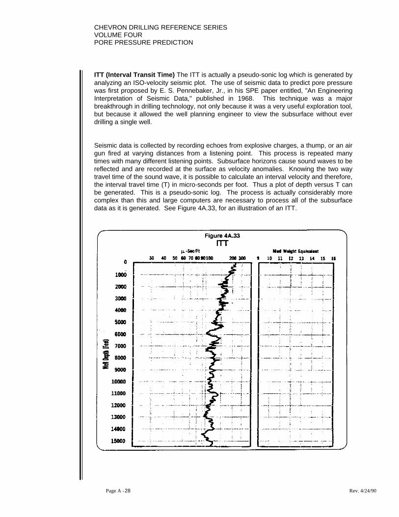
ITT (Interval Transit Time) The ITT is actually a pseudo-sonic log which is generated byanalyzing an ISO-velocity seismic plot. The use of seismic data to predict pore pressurewas first proposed by E. S. Pennebaker, Jr., in his SPE paper entitled, "An EngineeringInterpretation of Seismic Data," published in 1968. This technique was a majorbreakthrough in drilling technology, not only because it was a very useful exploration tool,but because it allowed the well planning engineer to view the subsurface without everdrilling a single well.
Seismic data is collected by recording echoes from explosive charges, a thump, or an airgun fired at varying distances from a listening point. This process is repeated manytimes with many different listening points. Subsurface horizons cause sound waves to bereflected and are recorded at the surface as velocity anomalies. Knowing the two waytravel time of the sound wave, it is possible to calculate an interval velocity and therefore,the interval travel time (T) in micro-seconds per foot. Thus a plot of depth versus T canbe generated. This is a pseudo-sonic log. The process is actually considerably morecomplex than this and large computers are necessary to process all of the subsurfacedata as it is generated. See Figure 4A.33, for an illustration of an ITT.

CHEVRON DRILLING REFERENCE SERIESVOLUME FOUR
PORE PRESSURE PREDICTION
Page A - 29 Rev. 4/24/90
A natural problem does exist in the science of interpreting seismic data. Sound wavestraveling through the subsurface tend to echo and re-echo causing multiples (echoes thatreoccur at regular intervals). However, careful examination of an ITT can indicate apossible transition zone and quantity pore pressure. Seismic processing and specificallyITT’s are very useful for the drilling engineer and every effort should be made to obtainthis information. Transition zone recognition is only one of several bits of informationwhich may be obtained. Known formation pressures in a previously drilled well can becorrelated across relatively long distances using several seismic sections. This may giveat least one positive control point for pore pressure in what might otherwise be acompletely unknown environment. Seismic data processing is a fairly complex scienceand every drilling engineer should make an effort to obtain as much information on thesubject as possible.
In summary, well planning actually requires an exhaustive research effort on the part ofthe drilling engineer. All possible sources of data and information must be employed. Itis simply not always sufficient to drill a new well just as we've drilled the last severalwells. Even with all pertinent information available and the best engineering toolsemployed, any well plan is still only a guide and the drilling fluid schedule is only anestimate. The man drilling the well must use these bits of information as tools andmodify the procedure as the well dictates. Recognizing "real time" indicators of abnormalpressure and combining these with a highly researched and engineered drilling programis the key to safe, efficient drilling operations.
7. Abnormal Pressure Indicators While Drilling
The recognition of real-time abnormal pressure indicators is extremely important indetermining when to weight-up the fluid system, where casing must be set, and to ensurethe drilling of a safe and efficient well. (Figure 4A. 34) It is important to note that theseindicators, along with the drilling plan, are both necessary tools for optimum efficiency.Furthermore, drilling indicators or signs of abnormal pressure hardly ever occur asisolated events. More often than not several, if not all of these events, will occur at thesame time. The following is a partial list and discussion of several abnormal pressureindicators.
Figure 4A.34
Abnormal Pressure IndicatorsWhile Drilling
• • Gas Cut Fluid• • Shale Problems• • Drilling Breaks• • "d" Exponent• • Temperature Anomalies

CHEVRON DRILLING REFERENCE SERIESVOLUME FOURPORE PRESSURE PREDICTION
Page A - 30 Rev. 4/24/90
8. Gas Cut Drilling Fluid
Gas cut fluid can, and often does indicate abnormal formation pressure. It is not,however, always necessary to weight-up the fluid system when an increase in background gas is recorded. Several circumstances need to be considered before any drasticmeasures are taken. The abnormal formation pressure may in fact be present but maynot be a problem. Many times tight shale segments may contain gas under pressure, butbecause the shale is tight (little or no permeability), the gas will not f low but is drilled upwhen the bit penetrates the rock. This does cause an increase in background gas, butcertainly does not constitute a well control problem. It can, and will, if a permeable sand,under the same pressure considerations, is penetrated by the bit. Circulating “bottomsup" and observing a return to normal background gas is the general procedure forhandling this type of concern. Other concerns are trip gas and connection gas. In bothcases, an influx of formation gas is noted due to a reduction in bottom hole pressure.This is caused by the absence of circulating pressure losses when the pump is shutdown, or the swabbing action created when the bit is pulled off bottom.
9. Shale Problems
Shale instability is often caused by an insufficient drilling fluid density. If the internal(pore) pressure of the shale is not at least balanced by the hydrostatic pressure of thedrilling fluid column, and the shale structure is weak or brittle, it will "pop" into thewellbore. These relatively large, angular and many times concave pieces of shale will bevery apparent on the shale shaker and can be indicative of abnormal or increasing porepressure. This situation may warrant increasing the fluid density or indicate that drillingshould be stopped in order to set casing.
Correct diagnosis of shale instability problems is complicated by the fact that cuttingsnearly identical to those described above can result from poor annular rheology andhydraulics which cause mechanical erosion. Excessive annular pressure lossescombined with a relatively long open hole exposure time can also cause severe shaleproblems. Under these conditions, increasing fluid density will actually compound theproblem. It should be obvious that an accurate assessment of this problem is necessaryprior to making any major changes. Sound preventative measures rather than correctivemeasures are really the keys.
10. Drilling Breaks

CHEVRON DRILLING REFERENCE SERIESVOLUME FOUR
PORE PRESSURE PREDICTION
Page A - 31 Rev. 4/24/90
It has been well established that as pore pressure increases, without a correspondingincrease in drilling fluid density, the drilling rate will also increase. This is due, in part, tothe fact that abnormally pressured formations are more porous and therefore, less densethan normally pressured formations.
When all drilling parameters are being held constant and a marked increase inpenetration rate occurs, a drilling break has been experienced. This may happen rapidlyand be very apparent or it can occur gradually. Nevertheless, drilling breaks are mostoften the first indicator that a transition from normal to abnormal pressure has occurred.A well researched drilling program will provide information that will indicate theapproximate depth of the transition zone and make recognition much easier.
11. "d" Exponents
The "d" exponent (Figure 4A.35) concept was developed as an attempt to quantifyformation drillability. A simplified drilling rate equation was modified so that an exponentdescribing the effect of weight on the bit, and conversely penetration rate, could be usedto indicate a normal shale compaction rate (Figure 4A.36). This then could be used tolocate transition zones and in some cases quantify pore pressure. It has someshortcomings in that drillability is also affected by hydraulics and mud, bit type and wear,and formation type (Figure 4A.37). The following equation was used to develop the "d"exponent.
Figure 4A.35
d-exponents
• • "Normalizes" Changesof WOB and RotarySpeed
Figure 4A.36
Penetration Rate
( )PR = k WOB
D rpm
d e×
×Figure 4A.37
DRILLABILITY (K)AFFECTED BY:
• • Hydraulics and Mud• • Bit Type and Wear
• • Formation

CHEVRON DRILLING REFERENCE SERIESVOLUME FOURPORE PRESSURE PREDICTION
Page A - 32 Rev. 4/24/90
R = K W N
D
d e
The parameters are defined as follows:
R = Penetration rate (ft/hr)K = A relative measure of formation drillability (dimensionless)W = Weight on Bit (Ibs/1000)D = Bit diameter (in)N = Rotary speed (rpm)d = An exponent to describe the effect of weight per inch of bit diameter or
penetration rate (dimensionless)e = An exponent to describe the effect of rotary speed on penetration rate
(dimensionless)
This basic drilling rate equation was modified based on the assumption that it would beused only in relatively homogeneous shale formations. With this assumption theformation drillability 'K' was set equal to 1 and the rotary speed exponent 'e' was setequal to 1 (Figure4A.38). These two assumptions are reasonable, provided that theformation is homogeneous (shale) and that rate of penetration is directly responsive torevolutions per minute. In other words, each bit revolution will penetrate one incrementof formation. The resulting equation is:
R = WD
N d
“d" now is a representative quantifier for formation hardness or drillability. Solving thesimplified drilling rate equation for "d" will yield the desired result.
R = WD
N d
RN
= WD
d
Log RN
= d Log W
D
CHEVRON DRILLING REFERENCE SERIESVOLUME FOUR
PORE PRESSURE PREDICTION
Page A - 33 Rev. 4/24/90
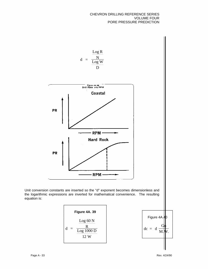
d =
Log RN
Log WD
Unit conversion constants are inserted so the “d" exponent becomes dimensionless andthe logarithmic expressions are inverted for mathematical convenience. The resultingequation is:
Figure 4A. 39
d =
Log 60 NR
Log 1000 D W12
Figure 4A.40
dc = d Gn
M.W.

CHEVRON DRILLING REFERENCE SERIESVOLUME FOURPORE PRESSURE PREDICTION
Page A - 34 Rev. 4/24/90
where:Gn = Normal formation pressure gradient (expressed in ppg)M.W. = Actual drilling fluid density (ppg)
One final correction is made which is difficult to justify mathematically, but does accountfor effects on drillability caused by drilling fluid properties. Drilling fluid density isassumed to have the greatest affect on drillability. The calculated “d” exponent is,therefore, multiplied by the ratio of the normal pressure gradient (usually expressed inppg) to the actual drilling fluid density (also expressed in ppg). This is called thecorrected “d” exponent and termed “dc” (Figure 4A.40).
This is a linear correction applied to an exponential function, however, for its intendeduse it turns out to be a very applicable tool.
Qualitatively, the "dc" will respond to normal compaction in the same way that resistivitydoes. The "dc" exponent will tend to increase with depth through normally pressuredsediments and decrease in under-compacted or abnormally pressured zones. In somecases, when "dc" data is to be correlated with conductivity or sonic log data, thereciprocal of “'dc" is multiplied by 100. This generates a"100/dc" plot. This plot of"l00/dc" will indicate a decreasing trend line through normal pressure, and an increasingtrend in abnormal pressure.
The "dc" or “l00/dc" plot will do an excellent job of identifying a transition zone. It willhowever, tend to over-estimate pore pressure as the actual drilling fluid densityincreases. This makes the prediction of pore pressure somewhat inaccurate especially inhigh pressure environments. Nevertheless, the "dc" exponent is still one of the best "realtime" monitoring tools for changes in drillability and, therefore,. transition zonerecognition.
Generally "dc" exponents should be calculated every ten feet, averaged over each fiftyfoot interval and then plotted. Data points will exhibit less scatter if the shale is relativelyclean and homogeneous. Relatively constant weight on bit, rotary speed and hydraulicswill all contribute to a more accurate and reliable plot as they all affect drill rate (Figure4A.41).
CHEVRON DRILLING REFERENCE SERIESVOLUME FOUR
PORE PRESSURE PREDICTION
Page A - 35 Rev. 4/24/90
Temperature anomalies.Temperature gradientincreases have already beenmentioned and discussed inthe section on shale propertytrends. At this point, it issufficient to say that flow linetemperature will definitelyincrease when an abnormallypressured environment isdrilled. This is due to the factthat the high pressure
environment is more porous and therefore, acts as a poorer heat exchanger than themore compacted surrounding sediments.
Heat is actually passed through the more porous sediments much slower and therefore,creates a higher wellbore temperature when those sediments are penetrated. Thesurface response to this phenomena is not immediate, however the information is usefuland flow line temperature should always be monitored.
12. AFTER DRILLING
After drilling the well, every effort should be made to obtain accurate pressure data forfuture drilling information (DST data, RFT's, Pressure bombs, Wireline Logs, etc.) (Figure4A.42).
ROCK FRACTURE MECHANISMS
Figure 4A.41
Factors Effecting Drill Rate
• • WOB• • RPM• • Hydraulics and Mud• • Bit Type and Wear• • Formation• • Differential Pressure
Figure 4A.42
After Drilling
• • Drill Stem Test• • Shut-In-Test• • Pressure
CHEVRON DRILLING REFERENCE SERIESVOLUME FOURPORE PRESSURE PREDICTION
Page A - 36 Rev. 4/24/90
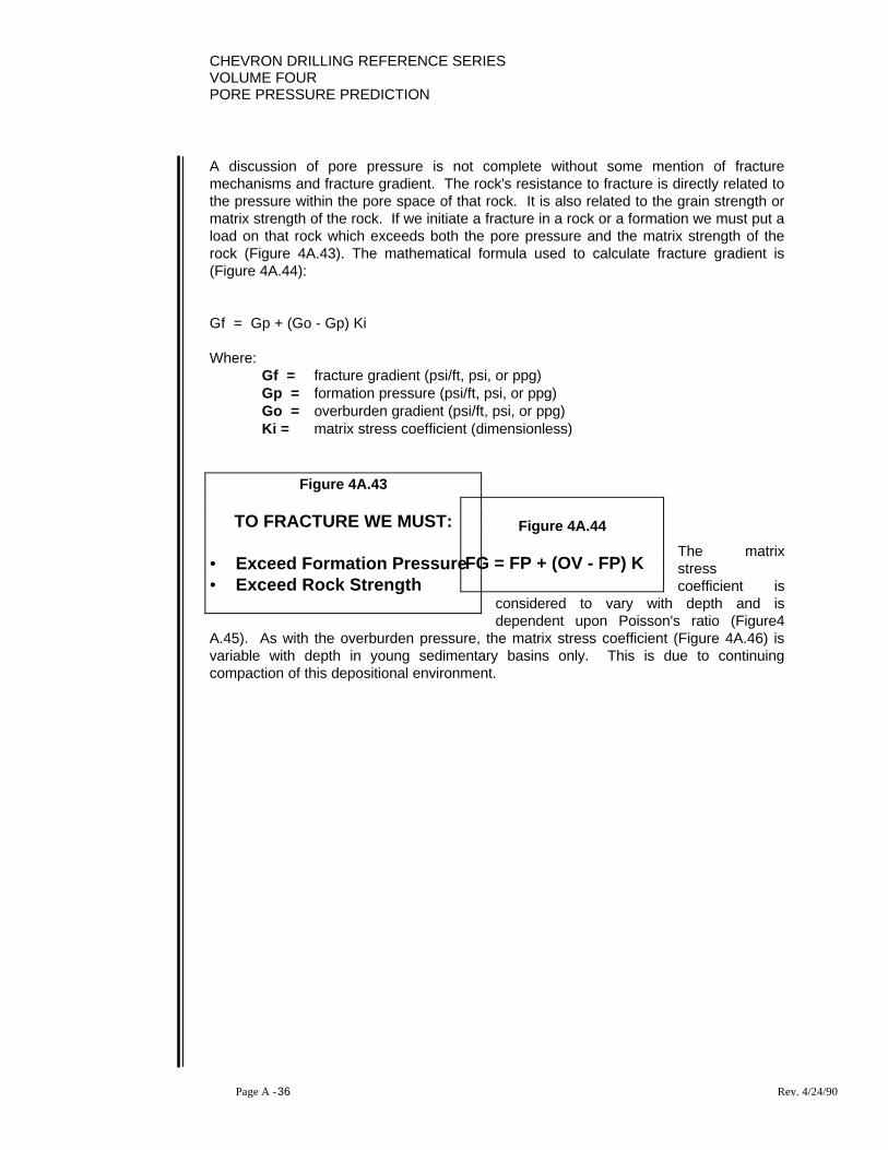
A discussion of pore pressure is not complete without some mention of fracturemechanisms and fracture gradient. The rock's resistance to fracture is directly related tothe pressure within the pore space of that rock. It is also related to the grain strength ormatrix strength of the rock. If we initiate a fracture in a rock or a formation we must put aload on that rock which exceeds both the pore pressure and the matrix strength of therock (Figure 4A.43). The mathematical formula used to calculate fracture gradient is(Figure 4A.44):
Gf = Gp + (Go - Gp) Ki
Where:Gf = fracture gradient (psi/ft, psi, or ppg)Gp = formation pressure (psi/ft, psi, or ppg)Go = overburden gradient (psi/ft, psi, or ppg)Ki = matrix stress coefficient (dimensionless)
The matrixstresscoefficient is
considered to vary with depth and isdependent upon Poisson's ratio (Figure4
A.45). As with the overburden pressure, the matrix stress coefficient (Figure 4A.46) isvariable with depth in young sedimentary basins only. This is due to continuingcompaction of this depositional environment.
Figure 4A.43
TO FRACTURE WE MUST:
• • Exceed Formation Pressure• • Exceed Rock Strength
Figure 4A.44
FG = FP + (OV - FP) K

CHEVRON DRILLING REFERENCE SERIESVOLUME FOUR
PORE PRESSURE PREDICTION
Page A - 37 Rev. 4/24/90
It is well to understand the difference between vertical and horizontal fractures and alsobetween true breakdown (fracture) pressure and fracture extension pressure. A briefdescription of each of these follows:
13. Horizontal Fractures
A horizontal fracture is possible at shallow depths and in very hard formations. Thedeeper the burial, the harder the formation must be in order to create a horizontalfracture. When the formation is competent enough to withstand pretrostatic pressure,
Figure 4A.46
Matrix Stress Coefficient, Ki
Dependent on Poisson's Ratio (v)Varies with Depth (young basins only)
Ki = V
1 - v

CHEVRON DRILLING REFERENCE SERIESVOLUME FOURPORE PRESSURE PREDICTION
Page A - 38 Rev. 4/24/90
fluid entering the formation may lift it vertically, thus creating a horizontal fractureextending laterally around the wellbore. This type of fracture is extremely rare in drilling,but has occurred.
14. Vertical Fractures
Vertical fractures are the most common. Rock will generally fail along a plane which isperpendicular to the plane of greatest stress. For most depositional environments thehorizontal stresses are greater than the vertical stress, therefore, the rock will have atendency to fracture in a vertical plane. The most likely place for any wellbore to fractureis immediately below the last casing seat. This is based on the fact that if normalcompaction has taken place, formations become harder and more dense as the depth ofburial increases. Therefore, the weakest point will be at the casing shoe. This is anidealization, and, of course, is not always true.
An important point to consider is that lost returns do in fact occur in shales, not in sand.This is true because shales are generally weaker than sands. Also, the minimalpermeability in shales will not allow fluid to enter them without causing a fracture. Left toset, both vertical and horizontal fractures tend to heal themselves in a "soft rock"environment. However, the time required for the healing process can be quite long.
15. Breakdown (Fracture) Pressure vs.Fracture Extension Pressure
As wells are drilled, and the time of open hole exposure increases, fluid from the wellboregradually seeps into sands and to a lesser degree shales. This seepage increases thehoop stress around the wellbore and also increases the pore pressure in the nearwellbore area. Understanding these facts certainly indicates that the fracture gradient willcorrespondingly increase as well. It is not uncommon to test a casing seat at one leak-off pressure and later retest it at a higher pressure. (Note that the leak off pressure isnot the same as the fracture (breakdown) pressure, but is still a measure of theformations strength).
Because of this, the true fracture (breakdown) pressure is generally higher than thefracture extension pressure (Figure 4A.47). Some test of formation integrity shouldalways be made (Figure 4A.48). If it is not desirable to go to a formation leak off, apressure test of some predetermined magnitude should be performed (Figure4A. 49). Inany event, formation integrity should be estimated prior to drilling, and measured forverification (Figure4A.50).
Prediction of Fracture Gradients

CHEVRON DRILLING REFERENCE SERIESVOLUME FOUR
PORE PRESSURE PREDICTION
Page A - 39 Rev. 4/24/90
There are two recommended methods to predict formation integrity (fracture gradient)prior to drilling the well and measuring it. The first method of predicting fracture gradientsis from charts developed by Mathews and Kelly or by Eaton. (Figure 4A.51).
Figure 4A.48
MEASUREMENT OF FRACTURE GRADIENT
• • Pressure Test
• • Leak Off Test

CHEVRON DRILLING REFERENCE SERIESVOLUME FOURPORE PRESSURE PREDICTION
Page A - 40 Rev. 4/24/90
Mathews and Kelly's charts assume a constant over-burden gradient of 19.23 ppg (1psi/ft) and empirically derived curves for a variable matrix stress coefficient, Ki. Thevalues obtained were used in the following equation:
FP = PP - Ki ( ob - PP )
Figure 4A.50
Ways to Obtain Fracture Gradients
• • Estimate from Charts
• • Measure

CHEVRON DRILLING REFERENCE SERIESVOLUME FOUR
PORE PRESSURE PREDICTION
Page A - 41 Rev. 4/24/90
Where:FP = Fracture Pressure (psi)PP = Pore Pressure (psi)Ki = Horizontal to vertical stress ratio (dimensionless)ob = Overburden stress (psi)
Figure 4A.51
Basic Differences
Overburden Matrix Stress (K)
Mathews and Kelly Constant Valve at19.23 ppg
Varies with Depth andArea
Eaton Varies with Depth andArea
Varies with Depth, andPoisson’s Ratio
Eaton’s work utilized Poisson’s Ratio to determine the relationship between horizontaland vertical rock matrix stresses and also used a variable overburden stress gradient.His work resulted in the following equation:
F = PP + V G D
1 - v - PP
ob sed××
Where:FP = Fracture Pressure (psi)PP = Pore Pressure (psi)V = Poisson's Ratio (dimensionless)Gob = Overburden Gradient (psi/ft)Dsed = Sediment Depth (ft)
This formula has been used to generate the chart shown in Figure 4A.52 and is probablythe most widely used predictive method in the industry today. These methods are similarin many ways but it is imperative that the use of either of these methods be on aconsistent basis. (i.e. DO NOT attempt to combine the two methods when predicting thefracture gradient for a proposed well. Doing so can result in large errors.)

CHEVRON DRILLING REFERENCE SERIESVOLUME FOURPORE PRESSURE PREDICTION
Page A - 42 Rev. 4/24/90
Both Mathews and Kelly's method and Eaton's method rely on regionally averaged dataand subsequently are in error for a given specific location. A more accurate techniqueinvolves the calculation of actual overburden stress values from open hole density logs.The logs may be offset well logs or logs derived from a specific drilling location. Thistechnique will result in a much more precise fracture pressure prediction for planningpurposes as well as real time prediction while the well is being drilled.
Deep Water Fracture Gradients
Experience has shown that as we begin to drill in deeper and deeper water, fracturegradients begin to decrease due to the reduction in overburden pressure (Figure 4A.53).As we move into deep water, a significant amount of the overburden becomes sea waterrather than soil (Figure 4A.54). This results in a significant loss of available fracturepressure and can become quite serious when drilling in very deep water (Figure 55).DTC Technical Memorandum 8802 proposes two methods to predict fracture gradientswhen drilling in water deeper than 350'.

CHEVRON DRILLING REFERENCE SERIESVOLUME FOUR
PORE PRESSURE PREDICTION
Page A - 43 Rev. 4/24/90

CHEVRON DRILLING REFERENCE SERIESVOLUME FOURPORE PRESSURE PREDICTION
Page A - 44 Rev. 4/24/90
Several final summary comments should be made concerning fracture gradient concepts.Given enough formation information, the overburden gradient, the matrix stresscoefficient and the pore pressure, one can calculate the fracture gradient using theincluded equations. Charts are available which graphically represent the same concept.Also, a relative measure of formation strength can be determined by performing a "leak-off" test. If done properly, a "leak-off" test does not fracture or break down the formation,but will indicate that pressure at which the formation will begin to take fluid. "Leak-off"tests should always be performed with high pressure, low volume pumping units.
Reasonably accurate fracture gradient estimations, regardless of the method(s) used,are very important for overall safe and efficient drilling operations. Experience hasindicated that with care, estimates can be within O.5 ppg of actual fracture extensionpressures. For "real time" operation sand well planning, this factor is significant andshould be kept in mind.

CHEVRON DRILLING REFERENCE SERIESVOLUME FOUR
PORE PRESSURE PREDICTION
Page A - 45 Rev. 4/24/90

CHEVRON DRILLING REFERENCE SERIESVOLUME FOURPORE PRESSURE PREDICTION
Page A - 46 Rev. 4/24/90
Figure 4A.56
Figure Pore Pressure PredictionFormula Summary
( )G = G - G - G RR
1.2p o o n
o
n
(Eaton - Resistivity)
Where: Gp = Pore Pressure (psi/ft, psi or ppg)Go = Overburden PressureGn = Normal PressureRo = Observed Resistivity (ohms m 2/m)Rn = Normal Resistivity (ohms m 2/m)
( )G = G - G - G CC
1.2p o o n
n
o
(Eaton - Conductivity)
Where: Co = Observed ConductivityCn = Normal Conductivity
( )G = G - G - G dd
1.2p o o n
co
cn
(Eaton - d exponents)
Where: dco = Observed dc exponentdcn = Normal dc exponent
( )G = G - G - G TT
3p o o nn
o
(Eaton - Sonic)
Where: Tn = Normal Interval Transit Time ( µ sec/ft)To = Observed Interval Transit Time ( µ sec/ft)
( )G = G - G - G D - D
D p n o n
i e
i
(Equivalent Depth)
Where: Di = Depth of Interest (ft)De = Equivalent Depth (ft)
Gf = Gp - ( Go - Gp ) Ki (Fracture Gradient)
Where: Gf = Fracture Gradient (psi/ft, psi or ppg)Ki = Matrix Stress Coefficient
CHEVRON DRILLING REFERENCE SERIESVOLUME FOUR
PORE PRESSURE PREDICTION
Page A - 47 Rev. 4/24/90
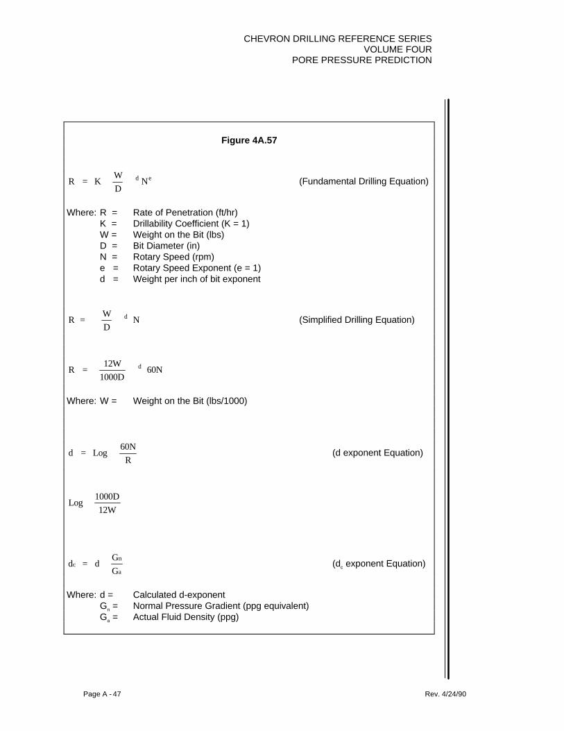
Figure 4A.57
R = K WD
Nd e
(Fundamental Drilling Equation)
Where: R = Rate of Penetration (ft/hr)K = Drillability Coefficient (K = 1)W = Weight on the Bit (lbs)D = Bit Diameter (in)N = Rotary Speed (rpm)e = Rotary Speed Exponent (e = 1)d = Weight per inch of bit exponent
R = WD
Nd
(Simplified Drilling Equation)
R = 12W
1000D 60Nd
Where: W = Weight on the Bit (lbs/1000)
d = Log 60N
R
(d exponent Equation)
Log 1000D12W
d = d GG
c n
a
(dc exponent Equation)
Where: d = Calculated d-exponentGn = Normal Pressure Gradient (ppg equivalent)Ga = Actual Fluid Density (ppg)
CHEVRON DRILLING REFERENCE SERIESVOLUME FOURPORE PRESSURE PREDICTION
Page A - 48 Rev. 4/24/90

CHEVRON DRILLING REFERENCE SERIESVOLUME FOUR
PORE PRESSURE PREDICTION
Page A - 49 Rev. 4/24/90
15. SUMMARY COMMENTS
The foregoing discussion of pore pressure prediction is by no means all inclusive. Itdoes, however, provide the fundamental tools and concepts for practical application bothfor well planning and the actual drilling operation.
In actuality, pore pressure prediction is very much a combination of engineeringapplication and an art form. There are two key factors that will play a major role in theaccuracy of any drilling plan which is based upon pore pressure development. First, thevolume and accuracy of the off set data available is critical. The more specific dataacquired, the more accurate the well plan will be. Secondly, the experience of theengineer doing the design is very important. It takes time to develop skill as a wellplanner. Much of the data used is subject to interpretation, and, therefore, correctjudgments are not always made the first or second time. Many normal trend lines mustbe drawn before accuracy can be expected.
One final idea should be mentioned. The purpose of all well planning when centeredaround development drilling projects, is to drill wells safer and more efficient thanprevious efforts have allowed. The well plan or design is only a tool to be used as aguide by the drilling representative on location. True drilling efficiency and optimizationcan only occur when the man drilling the well has a strong fundamental knowledge ofpore pressure, and has at his disposal a well researched and engineered drilling plan.The fundamental equations employed in this research appear in Figures 4A.56 and4A.57.

CHEVRON DRILLING REFERENCE SERIESVOLUME FOURPORE PRESSURE PREDICTION
Page A - 50 Rev. 4/24/90
*Eaton**Mathews & Kelly
GULF COAST VARIABLE OVERBURDEN GRADIENTSAND VARIABLE MATRIX STRESS COEFFICIENTS
Depth (ft) Overburden (psi/ft)* Matrix Stress Coef. (Ki)**
2,000 0.8725 0.3002,500 0.8788 0.3603,000 0.8850 0.4103,500 0.8913 0.4554,000 0.8919 0.4904,500 0.9013 0.5305,000 0.9063 0.5605,500 0.9100 0.5856,000 0.9163 0.6106,500 0.9194 0.6357,000 0.9237 0.6557,500 09281 0.6738,000 0.9325 0.6908,500 0.9363 0.7059,000 0.9400 0.7209,500 0.9438 0.735
10,000 0.9469 0.74510,500 0.9500 0.76011,000 0.9533 0.77211,500 0.9575 0.78512,000 0.9606 0.79512,500 0.9638 0.80513,000 0.9669 0.81313,500 0.9694 0.82314,000 0.9725 0.83114,500 0.9750 0.84015,000 0.9775 0.84815,500 0.9800 0.85516,000 0.9825 0.86116,500 0.9850 0.86917,000 0.9875 0.87417,500 0.9894 0.88018,000 0.9919 0.88618,500 0.9933 0.89119,000 0.9958 0.89819,500 0.9975 0.90120,000 1.0000 0.908

CHEVRON DRILLING REFERENCE SERIESVOLUME FOUR
PORE PRESSURE PREDICTION
Page A - 51 Rev. 4/24/90
CHEVRON DRILLING REFERENCE SERIESVOLUME FOUR
PORE PRESSURE PREDICTION
Page B - 1 Rev. 4/24/90
SECTION B: SONIC LOG PLOTTING AND OVERLAYS
1. INTRODUCTION
The determination of formation pore pressures from log derived properties is a highlyused and accepted practice in the Gulf of Mexico. Such determinations in other parts ofthe U. S. and the world have generally been very difficult, if not impossible, in manyinstances. Failure to do so, in most cases, has led to extreme drilling difficulties orunsuccessful wells. Much of the time, high pressure shale sections have beenmisinterpreted as chemically sensitive formations requiring exotic mud chemistries andresulting in needless excessive expense.
We have developed a technique for the determination of formation pore pressures fromsonic log trends which is universally applicable. This approach has been utilized innumerous locations around the world with great success. The process will bedemonstrated in detail and several examples of results this achieved from wells aroundthe world will be presented.
In conjunction with this pore pressure determination process, a simple means of creatinga pore pressure overlay to interpret the data will be demonstrated. This aids in speed ofdeterminations and simplifies the analysis somewhat.
Before an estimation of anticipated pore pressures to be seen in a proposed drillingprospect can be made, determinations of actual pore pressures seen in offset wells isessential. These pore pressure determinations are therefore, essential to the efficientand successful drilling of a well, and this technique enables one to make them.
2. BACKGROUND
Porosity at a given depth is related to the overburden load above. The higher theoverburden, the lower the porosity. At the same given depth and overburden, ifabnormally pressured, the porosity would be higher than for normally pressured rock.For the same pore pressure increase to be seen at this depth in a lower overburdenenvironment, we would see a greater porosity increase with respect to a normallypressured rock accompanying it. Thus, the overburden load directly affects formationporosity. This in turn affects the relative spacing between pore pressure trend lines in anoverlay. Since the overburden varies from place to place, the trend line spacing varieswith ft. This leads to the need for area specific pore pressure overlays.
The trend line spacings can be developed through determination of the pore pressureexponents in the Eaton Equation 1. Developing an overlay simplifies the pore pressure
CHEVRON DRILLING REFERENCE SERIESVOLUME FOURPORE PRESSURE PREDICTION
Page B - 2 Rev. 4/24/90
determination process. Here lies the need for the determination of the pressure equationexponents and the development of an overlay specific for each area.
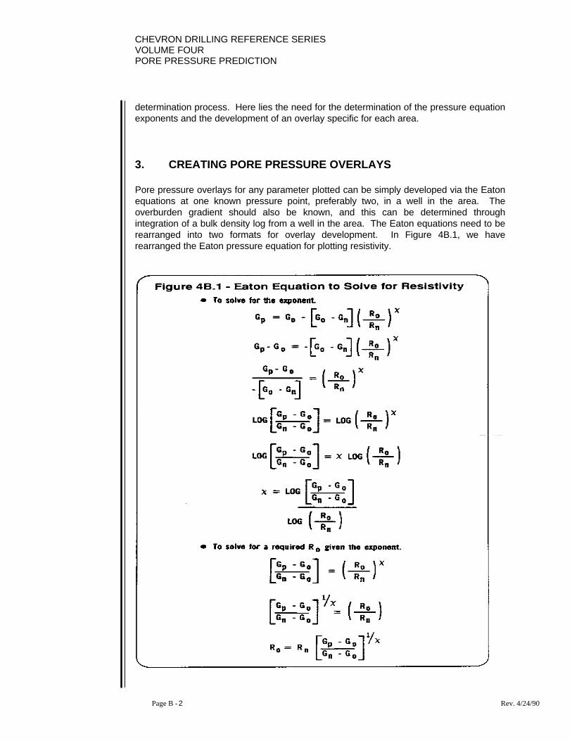
3. CREATING PORE PRESSURE OVERLAYS
Pore pressure overlays for any parameter plotted can be simply developed via the Eatonequations at one known pressure point, preferably two, in a well in the area. Theoverburden gradient should also be known, and this can be determined throughintegration of a bulk density log from a well in the area. The Eaton equations need to berearranged into two formats for overlay development. In Figure 4B.1, we haverearranged the Eaton pressure equation for plotting resistivity.

CHEVRON DRILLING REFERENCE SERIESVOLUME FOUR
PORE PRESSURE PREDICTION
Page B - 3 Rev. 4/24/90
Below, the equation is displayed in solving for the pressure exponent (x), and observedvalues of resistivity (Ro). Rearranging the Eaton pressure equation for plotting intervaltransit time appears in Figure 4B.2.
CHEVRON DRILLING REFERENCE SERIESVOLUME FOURPORE PRESSURE PREDICTION
Page B - 4 Rev. 4/24/90
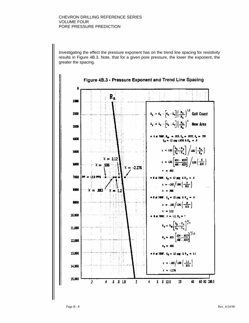
Investigating the effect the pressure exponent has on the trend line spacing for resistivityresults in Figure 4B.3. Note, that for a given pore pressure, the lower the exponent, thegreater the spacing.
CHEVRON DRILLING REFERENCE SERIESVOLUME FOUR
PORE PRESSURE PREDICTION
Page B - 5 Rev. 4/24/90
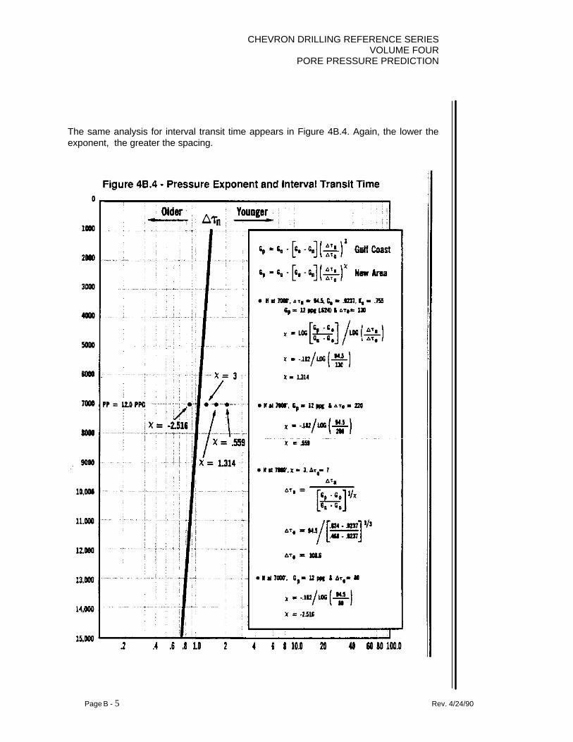
The same analysis for interval transit time appears in Figure 4B.4. Again, the lower theexponent, the greater the spacing.
CHEVRON DRILLING REFERENCE SERIESVOLUME FOURPORE PRESSURE PREDICTION
Page B - 6 Rev. 4/24/90
The process of creating an overlay first requires solving for the pressure exponent. Thisis done by plotting the log data of an offset well in which we have a known abnormalpressure point. From this we can determine a normal trend line for the parameterplotted. This normal trend line is extrapolated to the depth of the known abnormalpressure point to determine the normal value of this parameter. We have the observedvalue of the parameter associated with this abnormal pressure point from the log. Theoverburden gradient is determined through integration of the density log. We haveeverything but the exponent and this is obtained through the equation.
The remainder of the overlay creation process appears in Figure 4B.5. At a given depth,we assume the pore pressure to be abnormal values in 1 ppg increments and solve forthe observed value of the parameter of interest. These observed values associated withthe respective increments of pore pressure are plotted and trend lines are drawn throughthem parallel to the normal trend line established. Thus, we have created a porepressure overlay.

CHEVRON DRILLING REFERENCE SERIESVOLUME FOUR
PORE PRESSURE PREDICTION
Page B - 7 Rev. 4/24/90
4. TECHNIQUE FOR PLOTTING SONIC LOGS
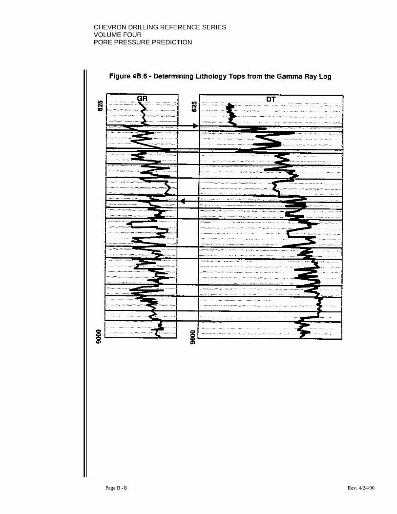
The first step is in determining lithology tops. This is done by displaying the gamma rayand sonic logs in a one inch equals one thousand foot scale. In compressing data likethis, a smoothing function need be applied to avoid a blur of data. Lithology tops arethen determined by picking the points where either the gamma ray or sonic shows achange in the general trend. This process is illustrated in Figures 4B.6 and 4B.7, withlithological tops indicated with the dark horizontal lines. The wells utilized in these twofigures are in Indonesia and Norway respectively.
CHEVRON DRILLING REFERENCE SERIESVOLUME FOURPORE PRESSURE PREDICTION
Page B - 8 Rev. 4/24/90

CHEVRON DRILLING REFERENCE SERIESVOLUME FOUR
PORE PRESSURE PREDICTION
Page B - 9 Rev. 4/24/90
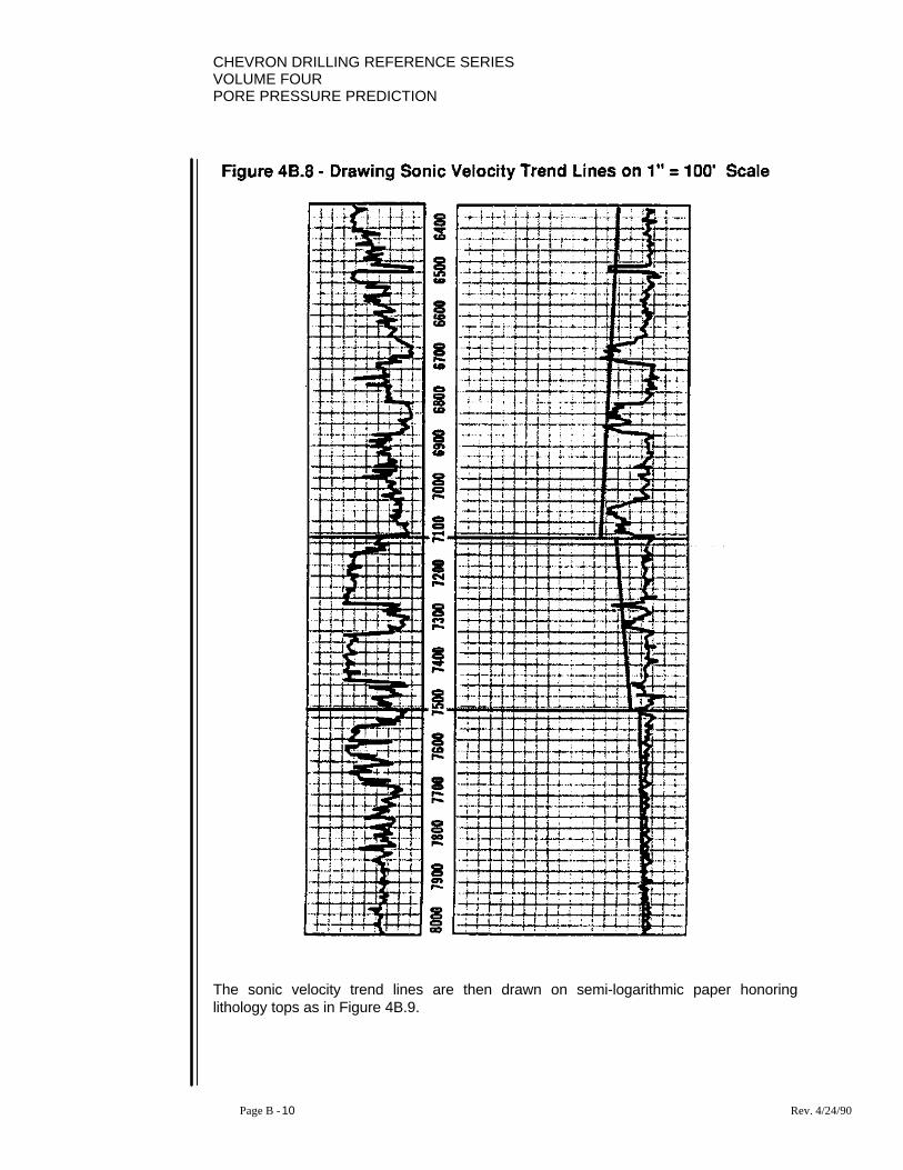
We will illustrate the process on the Indonesian well. The gamma ray and sonic are thendisplayed in a one inch equals one hundred foot scale. Again smoothing may berequired. The lithology tops previously determined are translated to this display. Sonicvelocity trend lines are then drawn on the sonic log with respect to the shale readingswithin lithological sections as illustrated in Figure 4B.8.
CHEVRON DRILLING REFERENCE SERIESVOLUME FOURPORE PRESSURE PREDICTION
Page B - 10 Rev. 4/24/90
The sonic velocity trend lines are then drawn on semi-logarithmic paper honoringlithology tops as in Figure 4B.9.

CHEVRON DRILLING REFERENCE SERIESVOLUME FOUR
PORE PRESSURE PREDICTION
Page B - 11 Rev. 4/24/90

CHEVRON DRILLING REFERENCE SERIESVOLUME FOURPORE PRESSURE PREDICTION
Page B - 12 Rev. 4/24/90
These lithology tops become recalibration points in this process. In this, the sonicvelocity trend in one lithological section is traced. The velocity trend is recalibrated byshifting the tracing over at the lithology change, joining the last value of interval velocity inthe last lithological section with the first value in the next. This results in a continuousrelative interval velocity profile as in Figure 4B.10.

CHEVRON DRILLING REFERENCE SERIESVOLUME FOUR
PORE PRESSURE PREDICTION
Page B - 13 Rev. 4/24/90
For this well we have a known formation pore pressure at 3800 feet of 10.6 ppgequivalent mud weight. We integrate the bulk density log and determine the overburdengradient. We now have what we need to solve for the pore pressure exponent andcreate an overlay for the area. This has been done as previously described in thecreation of pore pressure overlays in Figure 4B.11.

CHEVRON DRILLING REFERENCE SERIESVOLUME FOURPORE PRESSURE PREDICTION
Page B - 14 Rev. 4/24/90
Determination of pore pressure for all formations can now be read directly from theoverlay as in Figure 4B.12. Note that in the intervals which appear to have been drilledunder balanced, extreme difficulties with shale sloughing were encountered. All theformations encountered lacked permeability, except at TD where the mud weight had tobe raised to exceed the pore pressure.
CHEVRON DRILLING REFERENCE SERIESVOLUME FOUR
PORE PRESSURE PREDICTION
Page B - 15 Rev. 4/24/90
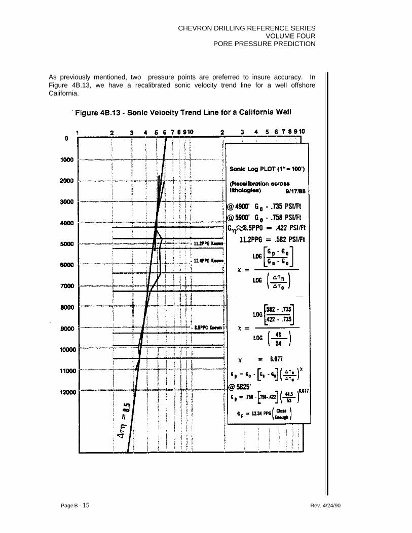
As previously mentioned, two pressure points are preferred to insure accuracy. InFigure 4B.13, we have a recalibrated sonic velocity trend line for a well offshoreCalifornia.

CHEVRON DRILLING REFERENCE SERIESVOLUME FOURPORE PRESSURE PREDICTION
Page B - 16 Rev. 4/24/90
In the California well illustrated on the previous page, we have two known abnormalpressure points. At 4900 feet we have an 11.2 ppg and at 5900 feet we have a 12.4 ppgpore pressure in mud weight equivalents. We solve for the exponent at 4900 feet wherewe have the 11.2 ppg. Using the exponent derived, we solve for pore pressure at 5900feet where we know the answer. As can be seen in Figure 4B.13 we get a pore pressureof 12.34 using the exponent in the Eaton pressure equation. Thus, we have confidencein the establishment of our normal trend line for this well and the determination of thepore pressure exponent for this area.
Again we can now create an overlay for use in all wells in the general area. By assumingvalues of abnormal pressure in increments of one ppg we solve for observed values ofsonic velocity utilizing the rearranged Eaton equation for sonic velocities as in Figure4B.14.
CHEVRON DRILLING REFERENCE SERIESVOLUME FOUR
PORE PRESSURE PREDICTION
Page B - 17 Rev. 4/24/90
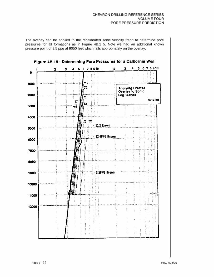
The overlay can be applied to the recalibrated sonic velocity trend to determine porepressures for all formations as in Figure 4B.1 5. Note we had an additional knownpressure point of 8.5 ppg at 9050 feet which falls appropriately on the overlay.
CHEVRON DRILLING REFERENCE SERIESVOLUME FOURPORE PRESSURE PREDICTION
Page B - 18 Rev. 4/24/90
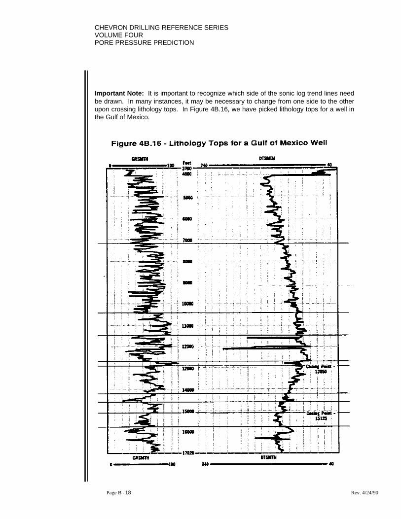
Important Note: It is important to recognize which side of the sonic log trend lines needbe drawn. In many instances, it may be necessary to change from one side to the otherupon crossing lithology tops. In Figure 4B.16, we have picked lithology tops for a well inthe Gulf of Mexico.

CHEVRON DRILLING REFERENCE SERIESVOLUME FOUR
PORE PRESSURE PREDICTION
Page B - 19 Rev. 4/24/90
We find in this well, from close examination of the sonic response with respect to theshales, that between the depths of 9300 and 10,400 feet, it becomes necessary to switchfrom plotting trend lines on the right to the left side of the sonic as illustrated in Figure 4B.17.
CHEVRON DRILLING REFERENCE SERIESVOLUME FOURPORE PRESSURE PREDICTION
Page B - 20 Rev. 4/24/90
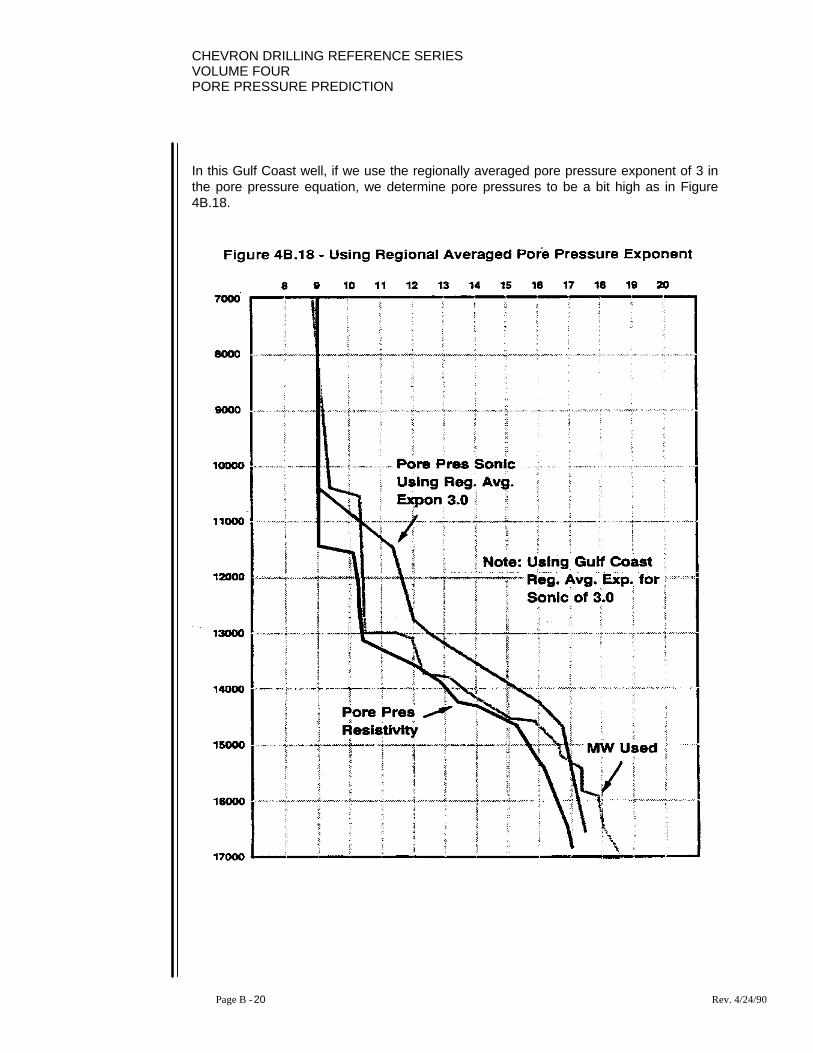
In this Gulf Coast well, if we use the regionally averaged pore pressure exponent of 3 inthe pore pressure equation, we determine pore pressures to be a bit high as in Figure4B.18.
CHEVRON DRILLING REFERENCE SERIESVOLUME FOUR
PORE PRESSURE PREDICTION
Page B - 21 Rev. 4/24/90
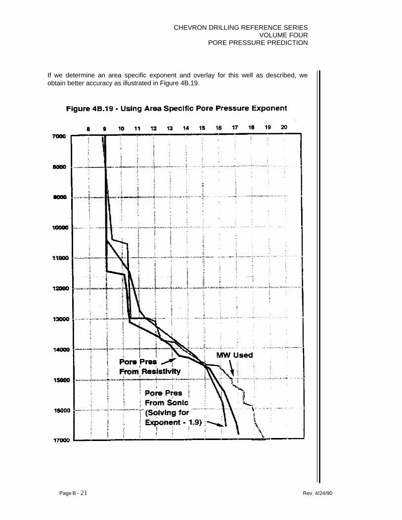
If we determine an area specific exponent and overlay for this well as described, weobtain better accuracy as illustrated in Figure 4B.19.
CHEVRON DRILLING REFERENCE SERIESVOLUME FOURPORE PRESSURE PREDICTION
Page B - 22 Rev. 4/24/90
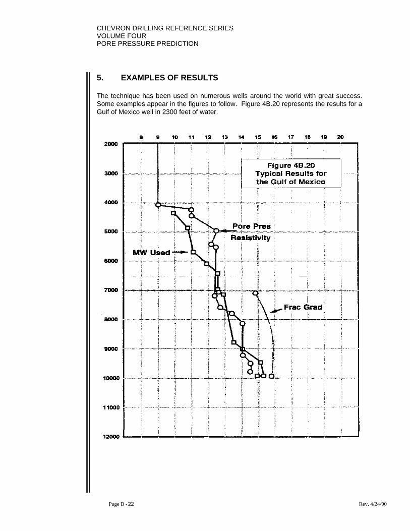
5. EXAMPLES OF RESULTS
The technique has been used on numerous wells around the world with great success.Some examples appear in the figures to follow. Figure 4B.20 represents the results for aGulf of Mexico well in 2300 feet of water.
CHEVRON DRILLING REFERENCE SERIESVOLUME FOUR
PORE PRESSURE PREDICTION
Page B - 23 Rev. 4/24/90
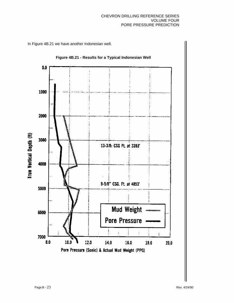
In Figure 4B.21 we have another Indonesian well.
Figure 4B.21 - Results for a Typical Indonesian Well

CHEVRON DRILLING REFERENCE SERIESVOLUME FOURPORE PRESSURE PREDICTION
Page B - 24 Rev. 4/24/90
Figure 4B.22 captures a well in Liberty County, Texas.
CHEVRON DRILLING REFERENCE SERIESVOLUME FOUR
PORE PRESSURE PREDICTION
Page B - 25 Rev. 4/24/90
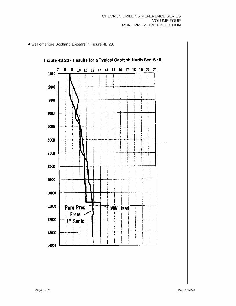
A well off shore Scotland appears in Figure 4B.23.

CHEVRON DRILLING REFERENCE SERIESVOLUME FOURPORE PRESSURE PREDICTION
Page B - 26 Rev. 4/24/90
The results for another well offshore Norway appears in Figure 4B.24.

CHEVRON DRILLING REFERENCE SERIESVOLUME FOUR
PORE PRESSURE PREDICTION
Page B - 27 Rev. 4/24/90
Pore Pressure Prediction Using Sonic Logs
Information Required:
1. Sonic logs from all Offset Wells displayed in True Vertical Depth with Gamma Rayand/or SP, preferably both. One set of logs should be displayed with a depthscale of 1" = 1000' and a second set displayed with a depth scale of 1” = 100'.Note that a smoothing function will be required for the 1” = 1000' log. Scale for thesonic should be linear with the majority of the plot using all of the area available(i.e. all four tracks).
2. Information as to where logging changes and casing points occurred (i.e. depths). 3. Any and all geologic data (i.e. location of faults in the area, cross-sections,
structure maps, etc.). 4. Mud, Bit and Drilling records from all offset wells to be analyzed.
Procedure:
1. Using the 1” = 1000 ft logs, identity intervals on the log where an abrupt shift insonic and/or gamma ray indicate a lithology change that is effecting the sonic.Draw a horizontal line through these points. These lines are referred to as "re-calibration points”.
2. Transfer the points identified in #1 to the 1” = 100 ft logs and note any changes in
log runs and casing points. Examine the log further to identify any additionallithology changes that might have been missed in #1. Draw horizontal linesthrough these points.
3. Draw trend lines connecting the sonic response in shales between the re-
calibration lines drawn in #2. Note: it is very important that the trend lines aredrawn on the correct side of the sonic plot. Examine the gamma ray plot and thesonic plot to determine the sonic response to the shales as compared to the otherlithology types. If the sonic response for a shale is to the left of that for thesurrounding non-shale lithologies, the trend lines should be drawn on the left sideof the plot. Conversely, if the shale response is to the right then the trend lineshould be drawn on the right side of the plot. The determination as to which sideof the plot the trend lines are drawn should be made for each interval between therecalibration points as the relationship between shales and non-shales can change
CHEVRON DRILLING REFERENCE SERIESVOLUME FOURPORE PRESSURE PREDICTION
Page B - 28 Rev. 4/24/90
with depth. The reason for the need to chose the correct side of the plot is that theslope of the trend line can change from one side of the plot to the other. If thewrong side is used it can result in errors for the remainder of the plot and adecrease in accuracy for the pore pressure prediction.
4. Transfer the trend lines and re-calibration points onto two cycle semi-log paper.
The easiest way to do this is to note the sonic values at the top and bottom ofeach trend line along with any inflections between the re-calibration points. Thenplot the same values on the semi-log paper. The typical depth scale used on thesemi-log paper is 1” = 1000 ft.
5. Overlay the semi-log paper with a second sheet of semi-log paper. Trace the
trendlines adjusting the top piece of paper to account for the shifting required toconnect the trendlines across the re-calibration points. It is very important that thetwo pieces of paper maintain the same orientation when shifting!!
6. Examine any additional data available in order to determine where the normal
trend line should be placed. Extend the normal trend line to the bottom of the plot. 7. If a regional overlay or an overlay from another offset wall is being used, place the
overlay on the plot created in #6, aligning the respective normal trend lines. Skipto step #9.
8. If an overlay is to be developed, note the depth and known pressure point(s) onto
the plot. Use Eaton's equations to determine the exponent and then calculate theobserved values for the various pore pressures. Plot these values onto the semi-log paper at the same depth for which the exponent was determined. Draw thetrend lines through these points parallel to the normal trend line determined in #6.
9. Read the pore pressure values at the inflection points and plot them on a pressure
vs. depth plot on regular coordinate paper.

CHEVRON DRILLING REFERENCE SERIESVOLUME FOUR
PORE PRESSURE PREDICTION
Page B - 29 Rev. 4/24/90
CHEVRON DRILLING REFERENCE SERIESVOLUME FOUR
PORE PRESSURE PREDICTION
Page C - 1 Rev. 4/24/90
SECTION C: PLOTTING RESISTIVITY LOGS FORFORMATION PORE PRESSUREDETERMINATIONS
1. INTRODUCTION
Techniques for estimating formation pore pressures from relative changes in log derivedshale properties have been in the industry and accepted for years. The basic premise, ofcourse, is that, at depth, shale porosity is a function of the pore fluid pressure and the logderived shale properties are a function of the shale porosity. There are difficulties,however, in that there are other factors which can influence the log properties of shalesthan just porosity alone. For this reason, the determination of formation pore pressuresfrom log properties can be difficult and inaccurate.
Recalibration techniques and considerations have been developed for the various logderived properties typically used in the industry, however, this paper will focus on thoseaffecting shale resistivity, or conductivity if you prefer. In particular, the effects ofchanges in formation salinities and the effects of multiple log runs are the significantfactors which have been addressed and dealt with. As increasing pore pressures areencountered, shale resistivities decrease as an indication of increasing pressure.However, if the formation water salinity increases, the shale resistivity will also drop,complicating the analysis. Also, as we set each string of casing, we log eachsubsequently smaller hole with a different log tool, probably a different logging engineerand in many cases with an entirely different logging unit. These changes which occur ateach log run also result in difficulty in pore pressure determinations across theseintervals.
This method addresses the effect of changing salinities and log runs and enables one toaccurately determine formation pore pressures from shale resistivity and conductivitytrends. The technique has been utilized on hundreds of wells throughout the Gulf ofMexico with great success. Typically pore pressure determinations are within a fewtenths of a pound per gallon of measured pore pressures in the adjacent virgin sands.
2. BACKGROUND
A method of determining formation pore pressure by analyzing log property trends wasdeveloped by Ben Eaton. With this technique we can plot shale values on a semi-logscale and determine a normal trend line through these values in the normally pressured,normally compacted section of the hole, as in Figure 4C.1.
By comparing shale properties which deviate from this normal trend to the values, atdepth, of the normal trend line, an estimation of pore pressure is made. The calculation
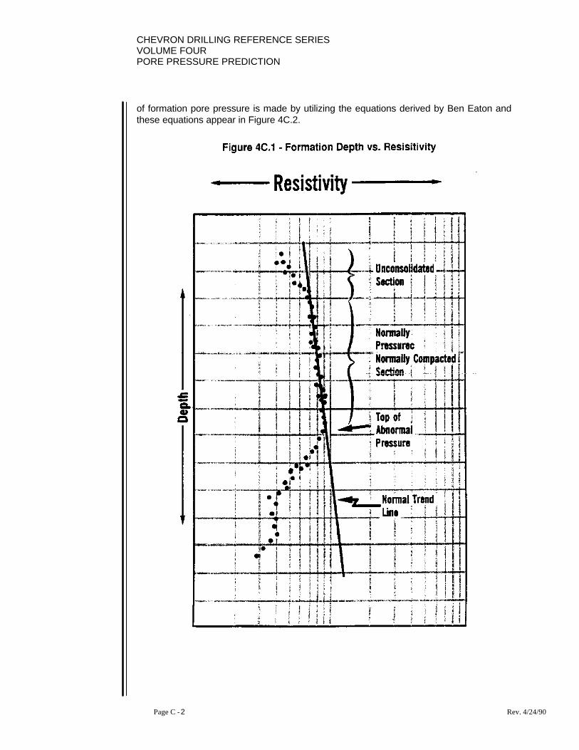
CHEVRON DRILLING REFERENCE SERIESVOLUME FOURPORE PRESSURE PREDICTION
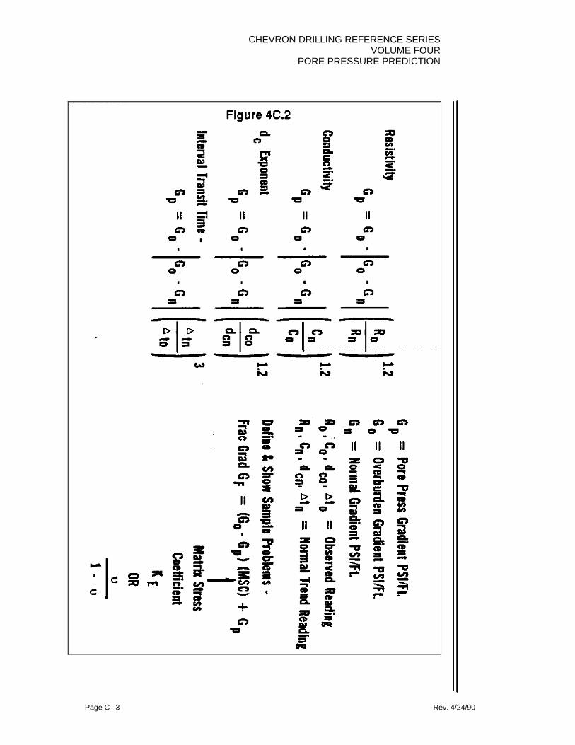
Page C - 2 Rev. 4/24/90
of formation pore pressure is made by utilizing the equations derived by Ben Eaton andthese equations appear in Figure 4C.2.
CHEVRON DRILLING REFERENCE SERIESVOLUME FOUR
PORE PRESSURE PREDICTION
Page C - 3 Rev. 4/24/90
CHEVRON DRILLING REFERENCE SERIESVOLUME FOURPORE PRESSURE PREDICTION
Page C - 4 Rev. 4/24/90
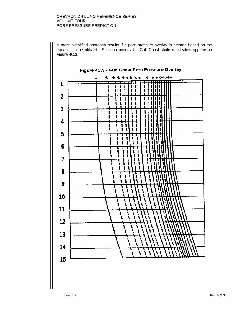
A more simplified approach results if a pore pressure overlay is created based on theequation to be utilized. Such an overlay for Gulf Coast shale resistivities appears inFigure 4C.3.

CHEVRON DRILLING REFERENCE SERIESVOLUME FOUR
PORE PRESSURE PREDICTION
Page C - 5 Rev. 4/24/90
With use of the overlay, the normal trend line of the overlay (9 ppg for the Gulf Coast) isaligned through the normally pressured normally compacted section of the hole and asshale properties deviate from this normal trend, a value of pore pressure is more simplyread from the overlay as in Figure 4C.4.
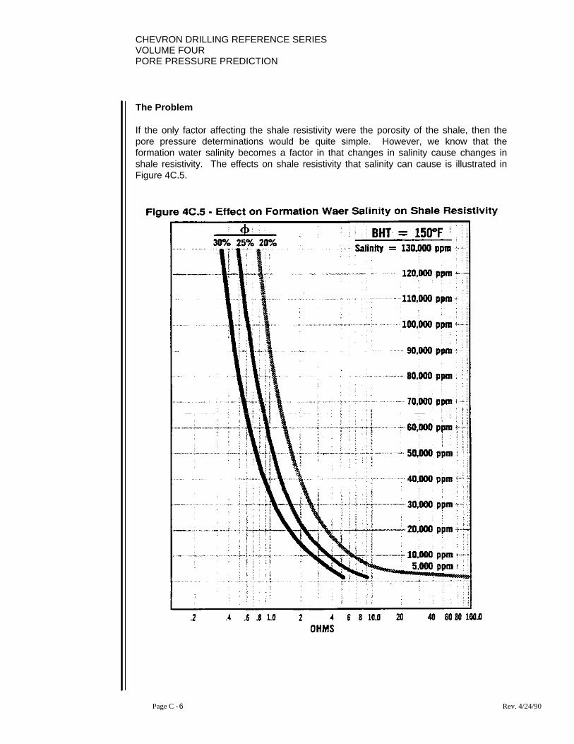
CHEVRON DRILLING REFERENCE SERIESVOLUME FOURPORE PRESSURE PREDICTION
Page C - 6 Rev. 4/24/90
The Problem
If the only factor affecting the shale resistivity were the porosity of the shale, then thepore pressure determinations would be quite simple. However, we know that theformation water salinity becomes a factor in that changes in salinity cause changes inshale resistivity. The effects on shale resistivity that salinity can cause is illustrated inFigure 4C.5.

CHEVRON DRILLING REFERENCE SERIESVOLUME FOUR
PORE PRESSURE PREDICTION
Page C - 7 Rev. 4/24/90
In addition, as we log each section of hole we use a different tool, a different loggingengineer, etc., and abrupt changes in shale resistivity can result as illustrated in Figure4C.6. We must, therefore, compensate for these factors if we are to accuratelydetermine formation pore pressures from log properties.
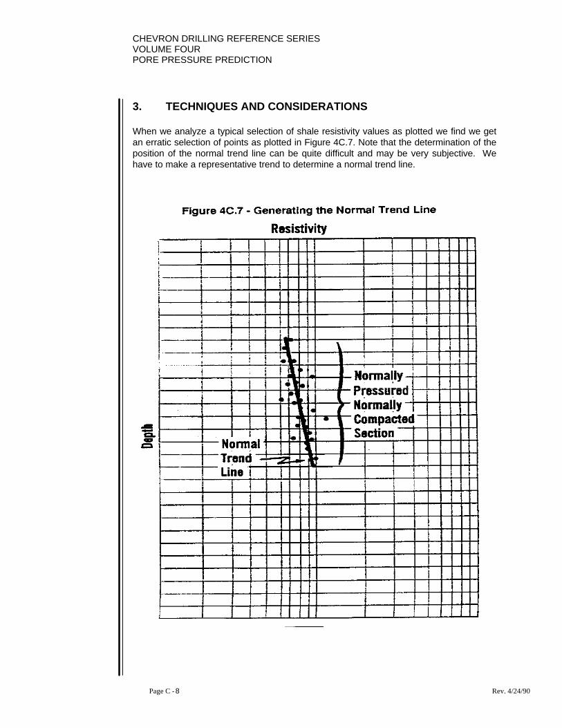
CHEVRON DRILLING REFERENCE SERIESVOLUME FOURPORE PRESSURE PREDICTION
Page C - 8 Rev. 4/24/90
3. TECHNIQUES AND CONSIDERATIONS
When we analyze a typical selection of shale resistivity values as plotted we find we getan erratic selection of points as plotted in Figure 4C.7. Note that the determination of theposition of the normal trend line can be quite difficult and may be very subjective. Wehave to make a representative trend to determine a normal trend line.
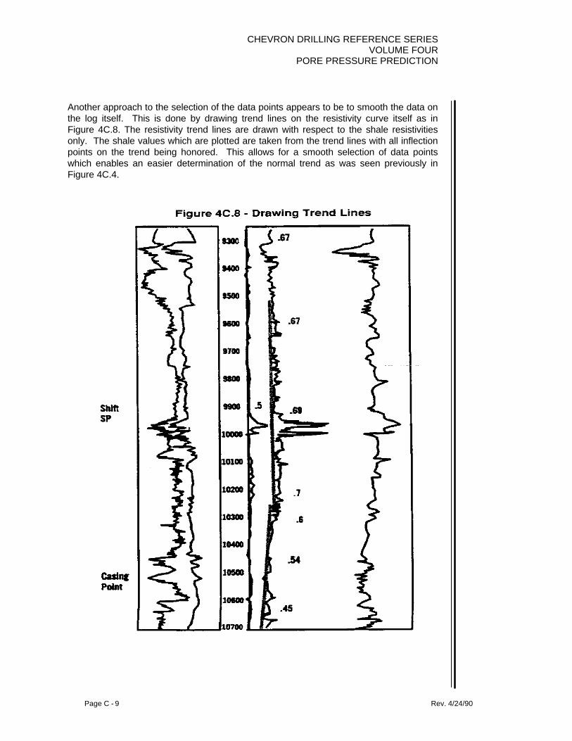
CHEVRON DRILLING REFERENCE SERIESVOLUME FOUR
PORE PRESSURE PREDICTION
Page C - 9 Rev. 4/24/90
Another approach to the selection of the data points appears to be to smooth the data onthe log itself. This is done by drawing trend lines on the resistivity curve itself as inFigure 4C.8. The resistivity trend lines are drawn with respect to the shale resistivitiesonly. The shale values which are plotted are taken from the trend lines with all inflectionpoints on the trend being honored. This allows for a smooth selection of data pointswhich enables an easier determination of the normal trend as was seen previously inFigure 4C.4.

CHEVRON DRILLING REFERENCE SERIESVOLUME FOURPORE PRESSURE PREDICTION
Page C - 10 Rev. 4/24/90
When we arrive at a change in log runs, at a casing point or otherwise, we mayencounter an abrupt change in the resistivity readings. One must be careful to selectvalid shale resistivity readings as close to the bottom of the previous log run, and asclose to the top of the next as possible and mark these points as recalibration points asin Figure 4C.9.
The recalibration process of these same data points appears in Figure 4C.10. Theoverlay is applied to the data aligning the 9 ppg trend line through the interval of pointswhich represent the normally pressured, normally compacted section of the hole. Porepressures are then read directly from the overlay below the normally pressured sectiondown to a recalibration point. Recalibration across this change in log runs is performedby shifting the overlay horizontally, without allowing any rotation, until the last reading ofpore pressure in the previous section coincides with the first reading of pore pressure inthe next section.

CHEVRON DRILLING REFERENCE SERIESVOLUME FOUR
PORE PRESSURE PREDICTION
Page C - 11 Rev. 4/24/90
In reference to Figure 4C.10, the last pore pressure reading was 12 ppg at approximately8200 feet. In this illustration, the overlay is shifted until the 12 ppg trend line is over thefirst valid shale resistivity reading. The recalibration process has taken place and valuesof pore pressure for this next section of hole are again read directly from the overlay tothe next recalibration point.

CHEVRON DRILLING REFERENCE SERIESVOLUME FOURPORE PRESSURE PREDICTION
Page C - 12 Rev. 4/24/90

CHEVRON DRILLING REFERENCE SERIESVOLUME FOUR
PORE PRESSURE PREDICTION
Page C - 13 Rev. 4/24/90

CHEVRON DRILLING REFERENCE SERIESVOLUME FOURPORE PRESSURE PREDICTION
Page C - 14 Rev. 4/24/90
Changes in formation water salinity also require the same recalibration procedure. Wehave a log section in Figure 4C.11 where such an abrupt salinity change occurs. Atapproximately 9520 feet, we cross a fault and see a significant salinity change. Note thedramatic change in shale resistivity above and below this point. As we plot the resistivityvalues as in Figure 4C.12, we indicate this point of salinity change as a recalibrationpoint.
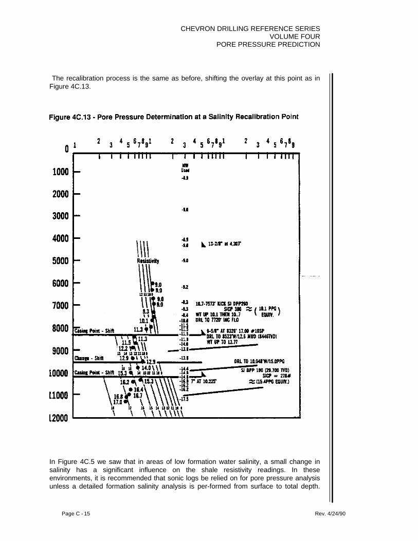
CHEVRON DRILLING REFERENCE SERIESVOLUME FOUR
PORE PRESSURE PREDICTION
Page C - 15 Rev. 4/24/90
The recalibration process is the same as before, shifting the overlay at this point as inFigure 4C.13.
In Figure 4C.5 we saw that in areas of low formation water salinity, a small change insalinity has a significant influence on the shale resistivity readings. In theseenvironments, it is recommended that sonic logs be relied on for pore pressure analysisunless a detailed formation salinity analysis is per-formed from surface to total depth.

CHEVRON DRILLING REFERENCE SERIESVOLUME FOURPORE PRESSURE PREDICTION
Page C - 16 Rev. 4/24/90
However, in areas of higher formation water salinities, such as the Gulf Coast, smallchanges do not have a dramatic impact on shale resistivity values, but large variationsdo.
CHEVRON DRILLING REFERENCE SERIESVOLUME FOUR
PORE PRESSURE PREDICTION
Page C - 17 Rev. 4/24/90
With this in mind, the primary concern is in recognizing when a significant salinity changehas occurred. To recognize such an occurrence, a simple technique can be applied. SPtrend lines can be drawn as well as resistivity trend lines on the log as in Figure 4C.14.The SP baseline will generally be affected significantly by two things; changes in salinity,and changes in shale porosity due to variations in pore pressure. When the formationpore pressures are increasing, the SP baseline will drift to the right in conjunction withresistivity drifting to the left. When this occurs the logging engineer will adjust the SPbaseline back to the left in order to prevent the SP curve from entering the depth track.Below this logger's adjustment, the SP will continue its right hand drift as pressurecontinues to build. This phenomena is illustrated in Figure 4C.15.

CHEVRON DRILLING REFERENCE SERIESVOLUME FOURPORE PRESSURE PREDICTION
Page C - 18 Rev. 4/24/90
However, a significant change in formation water salinity will be responded to by anabrupt shift in the SP baseline as has occurred in Figure 4C.16.
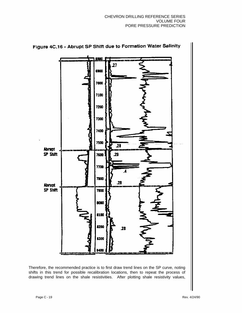
CHEVRON DRILLING REFERENCE SERIESVOLUME FOUR
PORE PRESSURE PREDICTION
Page C - 19 Rev. 4/24/90
Therefore, the recommended practice is to first draw trend lines on the SP curve, notingshifts in this trend for possible recalibration locations, then to repeat the process ofdrawing trend lines on the shale resistivities. After plotting shale resistivity values,

CHEVRON DRILLING REFERENCE SERIESVOLUME FOURPORE PRESSURE PREDICTION
Page C - 20 Rev. 4/24/90
overlay recalibration is performed only where the SP base line has shifted due toformation salinity changes as illustrated in Figure 4C.17.
If an overlay is not being used, these same recalibrations can be performed at changesin log runs and salinity by shifting the normal trend line an appropriate amount. This isprocess is illustrated in Figure 4C.18.
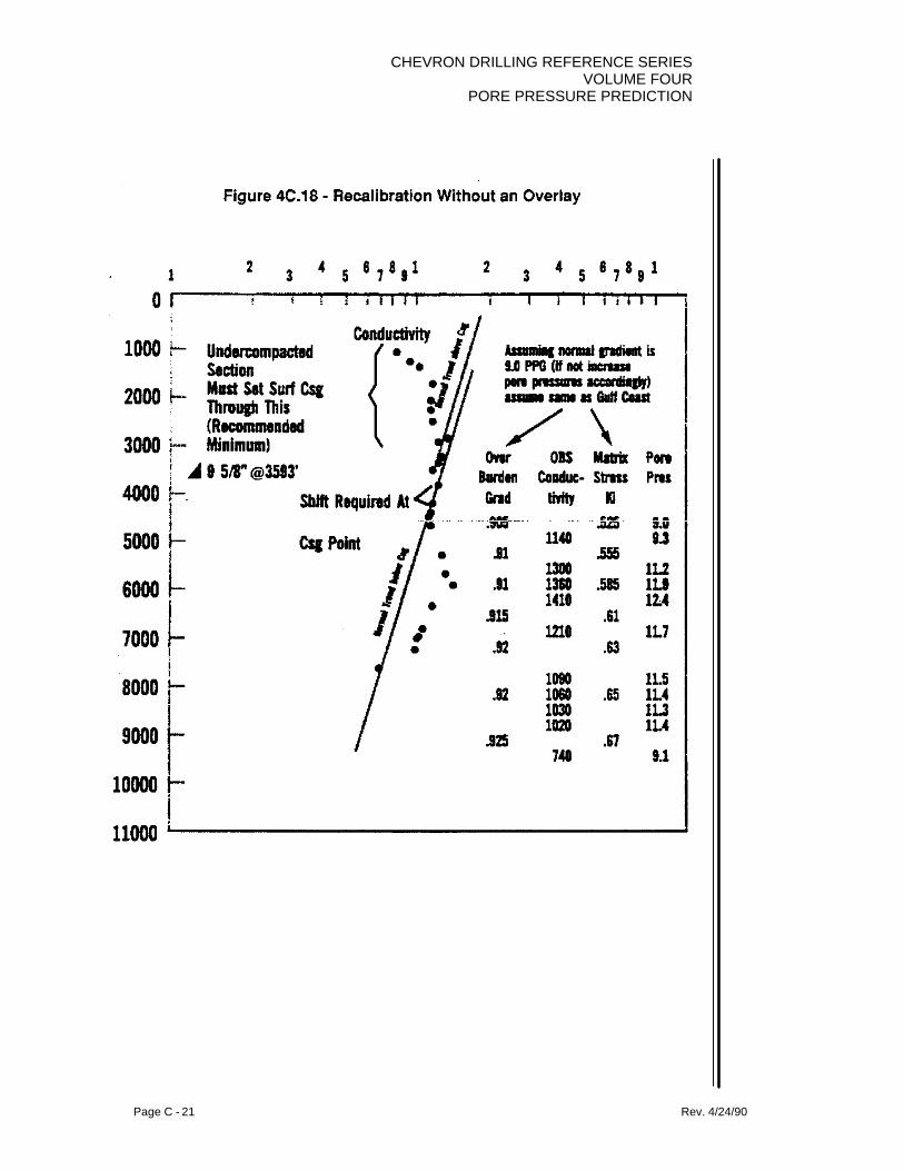
CHEVRON DRILLING REFERENCE SERIESVOLUME FOUR
PORE PRESSURE PREDICTION
Page C - 21 Rev. 4/24/90

CHEVRON DRILLING REFERENCE SERIESVOLUME FOURPORE PRESSURE PREDICTION
Page C - 22 Rev. 4/24/90
These techniques have been utilized on hundreds of wells throughout the Gulf of Mexicowith tremendous success and excellent accuracy. Typical results thus achieved areillustrated in Figures 4C.19 and 4C.20.

CHEVRON DRILLING REFERENCE SERIESVOLUME FOUR
PORE PRESSURE PREDICTION
Page C - 23 Rev. 4/24/90
CHEVRON DRILLING REFERENCE SERIESVOLUME FOURPORE PRESSURE PREDICTION
Page C - 24 Rev. 4/24/90
Pore Pressure Prediction using Resistivity Logs
Information Required:
1. Resistivity Logs for all Offset Wells displayed in True Vertical Depth with GammaRay and/or SP, preferably both. Scale should be 1” = 100 ft for the depth trackalthough 5” = 100 ft will work. Scale for the resistivity should be linear with themajority of the resistivity plot using all of the area available (i.e., all four tracks).
2. Information as to where logging changes and casing points occurred (i.e., depths). 3. Any and all geologic data (i.e., location of faults in the area, cross-sections, structure
maps, etc.) 4. Mud, Bit and Drilling records from all offset wells to be analyzed.
Procedure:
1. Note all log run changes and casing points on the resistivity logs. Examine the logsto determine any additional points where shifting is necessary (i.e., SP shifts).
2. Determine the shale response trend lines between the shift points. Trend lines forresistivity logs should always be drawn along the left side of the log trace.
3. Determine the resistivity values at each shift and inflection point and transpose thedata onto two cycle semi-log paper noting the shift points (i.e., recalibration points).
4. Overlay the semi-log paper with a second piece of semi-log paper of the same scale.Trace the trend lines adjusting the second piece of semi-log paper to account for theshifting required (i.e., connect the trend lines together by sliding the top sheet ofpaper), it is very important that the two pieces of paper remain the same orientationwhen the shifting is performed!!
5. Examine the drilling data available for the well in an effort to accurately determinewhere the normal trend line occurs. Pick the normal trend line and extend it to thebottom of the plot.
6. If the regional overlay or an overlay from another offset well is being used, place theoverlay on the plot created in #5 aligning the normal trend lines. Go to step #8.
7. If an overlay is to be created from the plot, note the depth and known pressurepoint(s) onto the plot. Use Eaton’s equations to determine the exponent and thencalculate the observed values for the various pore pressures. Plot these values ontothe semi-log paper at the same depth for which the exponent was determined. Drawtrend lines through these points parallel to the normal trend line determined by #5.
8. Read the pore pressure values at the inflection points and plot them on a Pressurevs. Depth plot on regular coordinate paper.
CHEVRON DRILLING REFERENCE SERIESVOLUME FOUR
PORE PRESSURE PREDICTION
Page C - 25 Rev. 4/24/90
CHEVRON DRILLING REFERENCE SERIESVOLUME FOURPORE PRESSURE PREDICTION
Page C - 26 Rev. 4/24/90

CHEVRON DRILLING REFERENCE SERIESVOLUME FOUR
PORE PRESSURE PREDICTION
Page D - 1 Rev. 4/24/90
SECTION D: DETERMINATION OF FORMATION POREPRESSURES IN CARBONATEENVIRONMENTS FROM SONIC LOGS
1. INTRODUCTION
Formation pore pressure determinations from log properties in carbonate environmentshave always been a difficult task. They do not compact uniformly with depth as doshales, nor is it necessarily true for the fluids to be in support of the overburden whenabnormally pressured, as in the classical sand shale abnormally pressured environment.Consequently, the traditional, somewhat straight forward, techniques of pore pressuredetermination from log properties do not, as such, apply.
We have developed an approach to determine formation pore pressures in carbonateenvironments utilizing sonic velocity trends. This technique has been utilized onapproximately 20 wells to date, as of this writing, with very good results. Wells analyzedhave ranged in pore pressures, at total depth, from 10 ppg to 18 ppg and have been asdeep as 23,000 feet. It has also been possible to identify pressure regressions.
The approach will be illustrated in detail, and the results of its use on a number of wellswill be presented, and explained. Mud weights required to drill these wells will also beillustrated as well as any pressure control data such as a kick.
2. BACKGROUND
In just about any environment, there tends to be a mixture comprising a rock's makeup.Generally speaking, in all sands there is some shale, in all shales there is some sand, inall carbonates there is some sand and shale and so forth. Thus, when we speak of arock as being a sandstone for instance, we are referring to its primary compositionalnature.
When we analyze a gamma ray log in a classical sand shale environment, we look for agamma ray response to the right for shale indication, and to the left for an indication ofsandstone.
When we analyze the gamma ray in a carbonate environment, the peak responses to theright are considered to be the result of shale within the rock matrix. It will be in theseintervals where we will concentrate our efforts.

CHEVRON DRILLING REFERENCE SERIESVOLUME FOURPORE PRESSURE PREDICTION
Page D - 2 Rev. 4/24/90
3. THE TECHNIQUE
The first step is in determining lithology tops. This is done by displaying the gamma rayand sonic logs in a one inch equals one thousand foot scale. In compressing data likethis, a smoothing function needs to be applied to avoid blurring the data. Lithology topsare then determined by picking the points where either the gamma ray or sonic shows achange in the general trend.
This process is illustrated in Figure 4D.1, with lithological tops indicated with the darkhorizontal lines. The well utilized in this Figure is in the Destin Dome area of the Gulf ofMexico.

CHEVRON DRILLING REFERENCE SERIESVOLUME FOUR
PORE PRESSURE PREDICTION
Page D - 3 Rev. 4/24/90
The gamma ray and sonic are then displayed in a one inch equals one hundred footscale. Again smoothing may be required. The lithology tops previously determined aretranslated to this display. Next to this data we display an unsmoothed version of thegamma ray, as well as an SP, resistivity and conductivity curves as in Figures 4D.2through 4D.6.

CHEVRON DRILLING REFERENCE SERIESVOLUME FOURPORE PRESSURE PREDICTION
Page D - 4 Rev. 4/24/90
Within lithological sections, we analyze the gamma ray peaks which trend to the right inthe shale direction. We've circled these in Figures 4D.2 through 4D.6.

CHEVRON DRILLING REFERENCE SERIESVOLUME FOUR
PORE PRESSURE PREDICTION
Page D - 5 Rev. 4/24/90
With respect to these gamma ray peaks to the right, we draw sonic log velocity trendlines, honoring the sonic velocities which correspond to the gamma ray intervalspreviously circled.
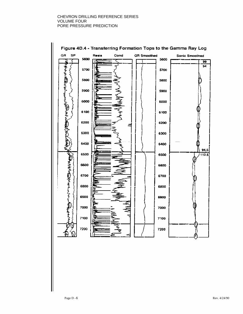
CHEVRON DRILLING REFERENCE SERIESVOLUME FOURPORE PRESSURE PREDICTION
Page D - 6 Rev. 4/24/90

CHEVRON DRILLING REFERENCE SERIESVOLUME FOUR
PORE PRESSURE PREDICTION
Page D - 7 Rev. 4/24/90
These corresponding sonic velocities have also been circled in Figures 4D.2 through4D.6 and the corresponding trend lines have been drawn.

CHEVRON DRILLING REFERENCE SERIESVOLUME FOURPORE PRESSURE PREDICTION
Page D - 8 Rev. 4/24/90
Note that in some instances in Figures 4D.2 through 4D.6 that the velocity trend linesappear on the left of the sonic log, and in others on the right.
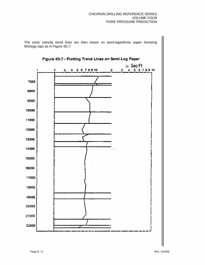
CHEVRON DRILLING REFERENCE SERIESVOLUME FOUR
PORE PRESSURE PREDICTION
Page D - 9 Rev. 4/24/90
The sonic velocity trend lines are then drawn on semi-logarithmic paper honoringlithology tops as in Figure 4D.7.

CHEVRON DRILLING REFERENCE SERIESVOLUME FOURPORE PRESSURE PREDICTION
Page D - 10 Rev. 4/24/90
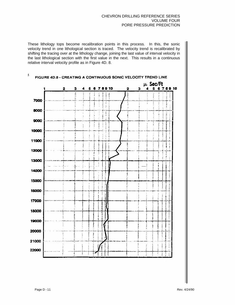
CHEVRON DRILLING REFERENCE SERIESVOLUME FOUR
PORE PRESSURE PREDICTION
Page D - 11 Rev. 4/24/90
These lithology tops become recalibration points in this process. In this, the sonicvelocity trend in one lithological section is traced. The velocity trend is recalibrated byshifting the tracing over at the lithology change, joining the last value of interval velocity inthe last lithological section with the first value in the next. This results in a continuousrelative interval velocity profile as in Figure 4D. 8.

CHEVRON DRILLING REFERENCE SERIESVOLUME FOURPORE PRESSURE PREDICTION
Page D - 12 Rev. 4/24/90
Note, in Figure 4D.9, that we can draw a normal trend line through the normallypressured, normally compacted section of the hole from 5400 to 8700 feet. For this wellwe have a known formation pore pressure at 21,000 feet of 15.2 ppg equivalent mudweight.

CHEVRON DRILLING REFERENCE SERIESVOLUME FOUR
PORE PRESSURE PREDICTION
Page D - 13 Rev. 4/24/90
We integrate the bulk density log and determine the overburden gradient. We now havewhat we need to solve for the pore pressure exponent and create an overlay for the area.This has been done in Figure 4D.10.
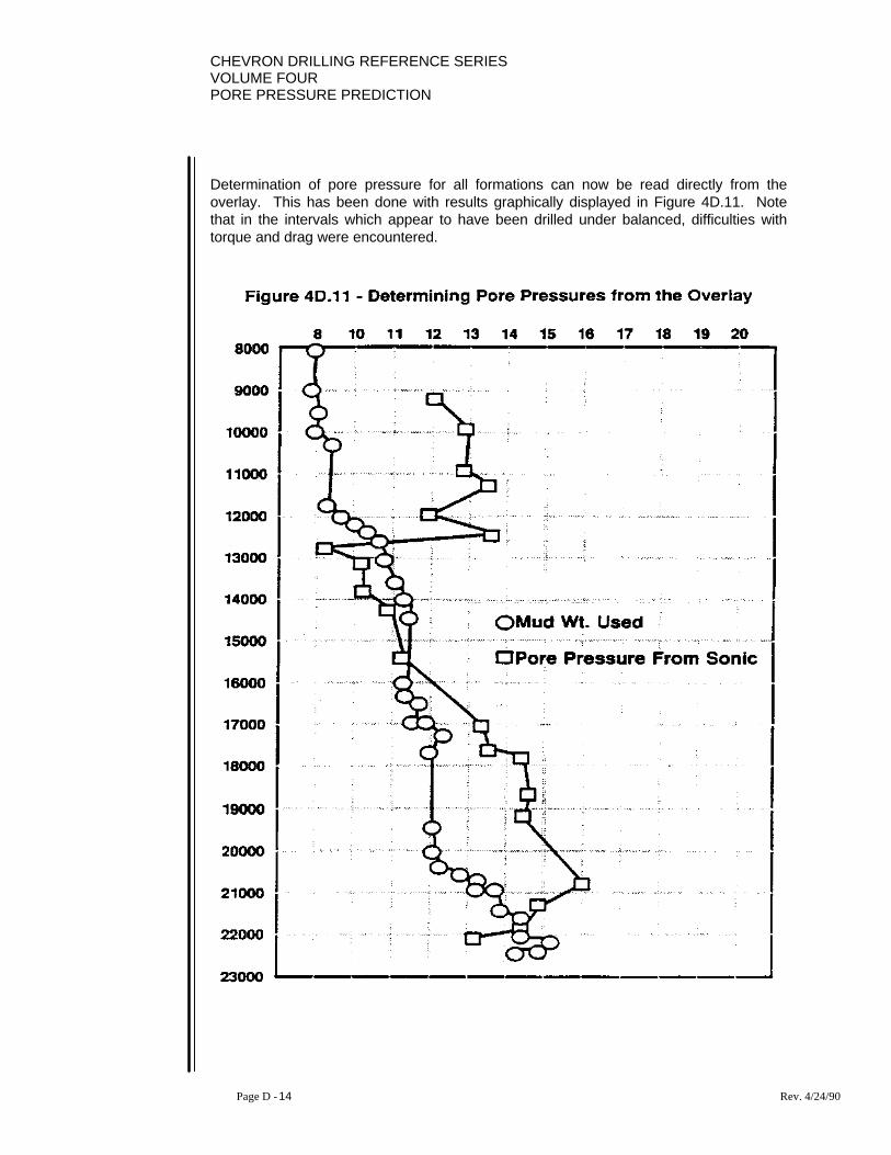
CHEVRON DRILLING REFERENCE SERIESVOLUME FOURPORE PRESSURE PREDICTION
Page D - 14 Rev. 4/24/90
Determination of pore pressure for all formations can now be read directly from theoverlay. This has been done with results graphically displayed in Figure 4D.11. Notethat in the intervals which appear to have been drilled under balanced, difficulties withtorque and drag were encountered.
CHEVRON DRILLING REFERENCE SERIESVOLUME FOUR
PORE PRESSURE PREDICTION
Page D - 15 Rev. 4/24/90
All the formations encountered lacked permeability, other than the formation at 21,000feet which was of low permeability. This formation of approximately 15.2 ppg porepressure continued to flow at a rate of roughly 3/4 a barrel per hour with a mud weight ashigh as 14.9 ppg in the hole. The bottom portion of the well experienced a pressureregression and mud weights could be reduced.
Additional Important Point
It is important to recognize which side of the sonic log trend lines need be drawn. Inmany instances, it may be necessary to change from one side to the other upon crossinglithology tops. In Figures 2 through 6, from close examination of the sonic response withrespect to the gamma ray intervals selected, it becomes necessary to switch fromplotting trend lines on the right to the left side of the sonic and vice-versa.
4. EXAMPLES OF RESULTS
The technique has been used on numerous wells with great success. Figures 4D.12through 4D.17 depict some of the results.
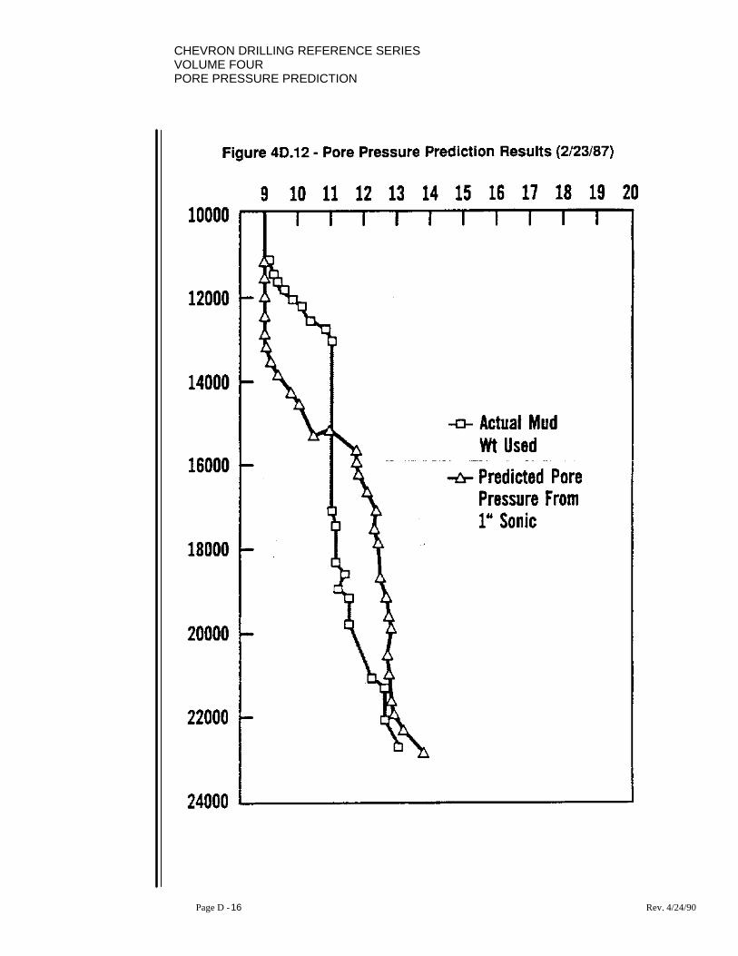
CHEVRON DRILLING REFERENCE SERIESVOLUME FOURPORE PRESSURE PREDICTION
Page D - 16 Rev. 4/24/90

CHEVRON DRILLING REFERENCE SERIESVOLUME FOUR
PORE PRESSURE PREDICTION
Page D - 17 Rev. 4/24/90

CHEVRON DRILLING REFERENCE SERIESVOLUME FOURPORE PRESSURE PREDICTION
Page D - 18 Rev. 4/24/90
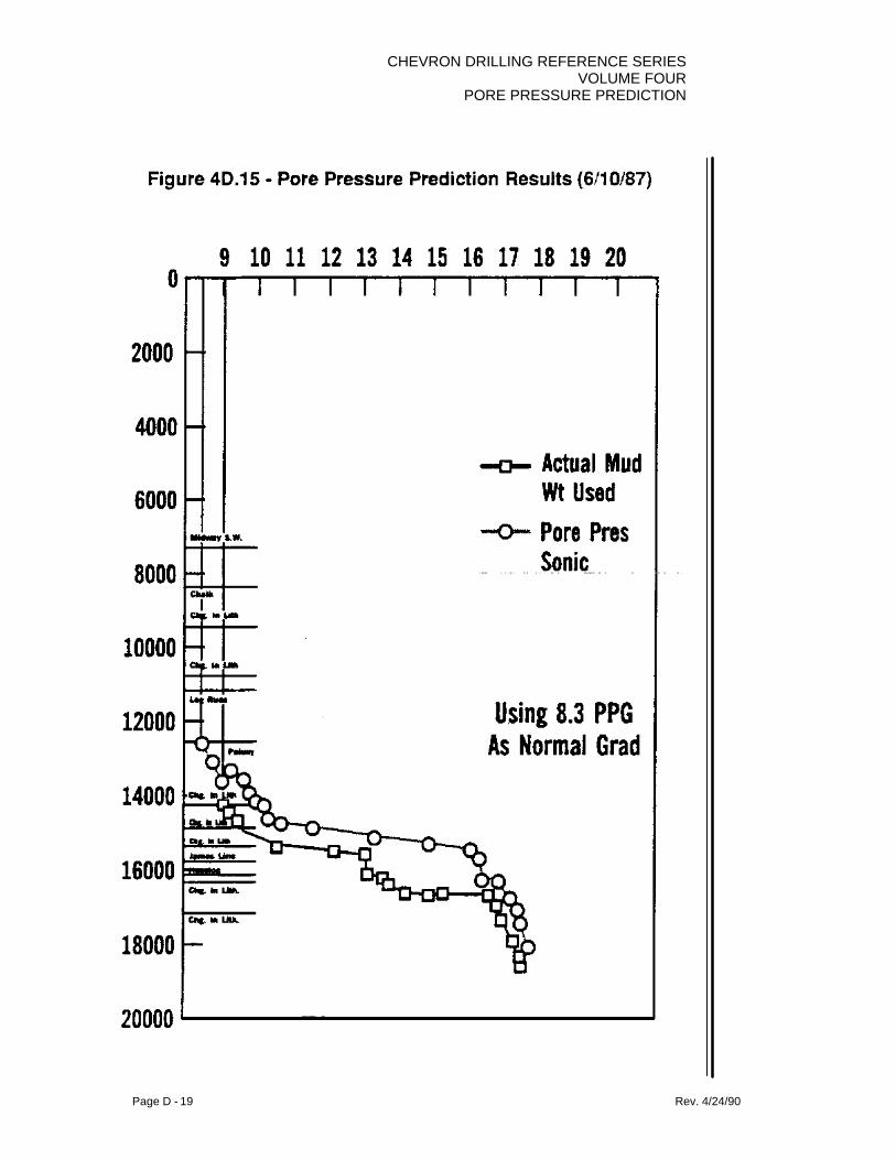
CHEVRON DRILLING REFERENCE SERIESVOLUME FOUR
PORE PRESSURE PREDICTION
Page D - 19 Rev. 4/24/90

CHEVRON DRILLING REFERENCE SERIESVOLUME FOURPORE PRESSURE PREDICTION
Page D - 20 Rev. 4/24/90
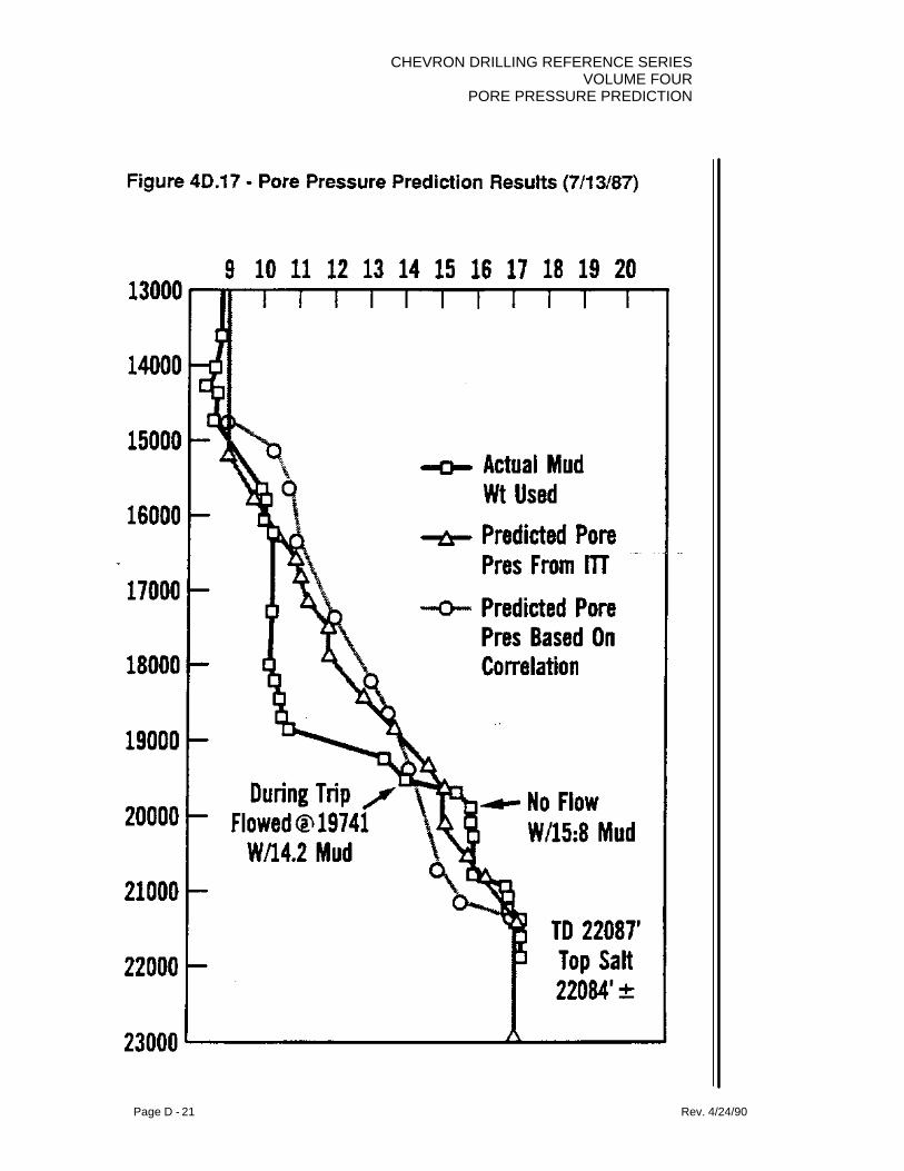
CHEVRON DRILLING REFERENCE SERIESVOLUME FOUR
PORE PRESSURE PREDICTION
Page D - 21 Rev. 4/24/90

CHEVRON DRILLING REFERENCE SERIESVOLUME FOURPORE PRESSURE PREDICTION
Page D - 22 Rev. 4/24/90

CHEVRON DRILLING REFERENCE SERIESVOLUME FOUR
PORE PRESSURE PREDICTION
Page E - 1 Rev. 4/24/90
SECTION E: THE EFFECTS OF STRUCTURAL CHANGESBETWEEN WELLS
For an oil field to develop, there are several things nature must have provided. Theremust be a source of the hydrocarbons. Hopefully these hydrocarbons migrate through areservoir type rock, having permeability and porosity, to a point where they becometrapped in some way by a capping formation.
Some typical traps seen around the world are in anticlinal structures, againstimpermeable formations such as salt domes, or against impermeable formations acrossa fault.
We gain an understanding of the look of the formations below the earth’s surface throughthe use of seismic surveys. An energy source is used to pulse sound waves through theearth. Some of the energy of these sound waves is bounced back at each formation topor lithological change as in Figure 4E.1.

CHEVRON DRILLING REFERENCE SERIESVOLUME FOURPORE PRESSURE PREDICTION
Page E - 2 Rev. 4/24/90
The results of this seismic survey yields a picture which approximates the generalizedshape of the formations below the earth’s surface as in Figure 4E.2.
The composition of formation clays can be significantly dependent upon the depth ofburial as in Figure 4E.3. As clays are subjected to ever increasing pressures andtemperatures due to deeper depths of burial resulting from additional sedimentation, theyexperience a metamorphosis. Montmorillonites convert to illites at deeper depths and soforth. The well on the right can penetrate a shale formation with the clay composition asshown. Upon drilling an offset well on the left, if this same stratigraphy is encountered atsome shallower depth, the shales may have undergone less change due to a loweroverburden load and temperature and we might see a somewhat different claycomposition. This can have an effect on the drilling fluid chemistry required to drill thisformation.
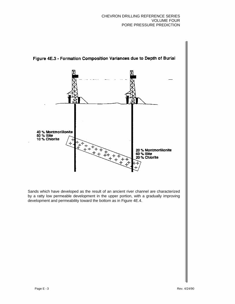
CHEVRON DRILLING REFERENCE SERIESVOLUME FOUR
PORE PRESSURE PREDICTION
Page E - 3 Rev. 4/24/90
Sands which have developed as the result of an ancient river channel are characterizedby a ratty low permeable development in the upper portion, with a gradually improvingdevelopment and permeability toward the bottom as in Figure 4E.4.

CHEVRON DRILLING REFERENCE SERIESVOLUME FOURPORE PRESSURE PREDICTION
Page E - 4 Rev. 4/24/90
Sands which have developed as the result of an ancient beach are characterized as tinegrained on bottom and coarse on top. These sands tend to gradually thin out and losedevelopment as we head seaward to the right in the illustration in Figure 4E.5.

CHEVRON DRILLING REFERENCE SERIESVOLUME FOUR
PORE PRESSURE PREDICTION
Page E - 5 Rev. 4/24/90
Many, if not most, ancient carbonates were deposited simultaneously in three differentmacro-environments; shelf, slope and basin as illustrated in Figure 4E.6. The shelfenvironment consists of broad, shallow seas, mostly less than 100 feet of water.Currents are weak, so generally lime mud has been deposited. Usually there is enoughcurrent or wave motion to keep the water oxygenated. Scattered isolated coral heads orlarger patch reefs are common. Sometimes in mud banks, oxygen is used up andorganic matter is preserved.
The material on the slope consists of lime sands and blocks that have been broken offthe reef by waves and deposited in strata with an initial dip. They are called reef talusand sometimes form excellent reservoirs.
The material in the basin is fine grained, usually lime mud. Normally, it does not havesufficient permeability to produce hydrocarbons. In a few places, chalk has accumulated,formed from the tiny shells of algae called coccoliths. They have considerable porositybut very low permeability. The basinal carbonates often grade laterally into shale. In thecase of epi-continental basins, it often happens that there is little circulation of the waterin the deeper parts of the basins. Organic matter is preserved because not enoughoxygen is brought in to destroy it. Occasionally such deposits become highly organic andmay become source rocks of hydrocarbons.

CHEVRON DRILLING REFERENCE SERIESVOLUME FOURPORE PRESSURE PREDICTION
Page E - 6 Rev. 4/24/90
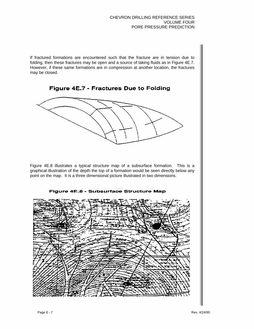
CHEVRON DRILLING REFERENCE SERIESVOLUME FOUR
PORE PRESSURE PREDICTION
Page E - 7 Rev. 4/24/90
If fractured formations are encountered such that the fracture are in tension due tofolding, then these fractures may be open and a source of taking fluids as in Figure 4E.7.However, if these same formations are in compression at another location, the fracturesmay be closed.
Figure 4E.8 illustrates a typical structure map of a subsurface formation. This is agraphical illustration of the depth the top of a formation would be seen directly below anypoint on the map. It is a three dimensional picture illustrated in two dimensions.
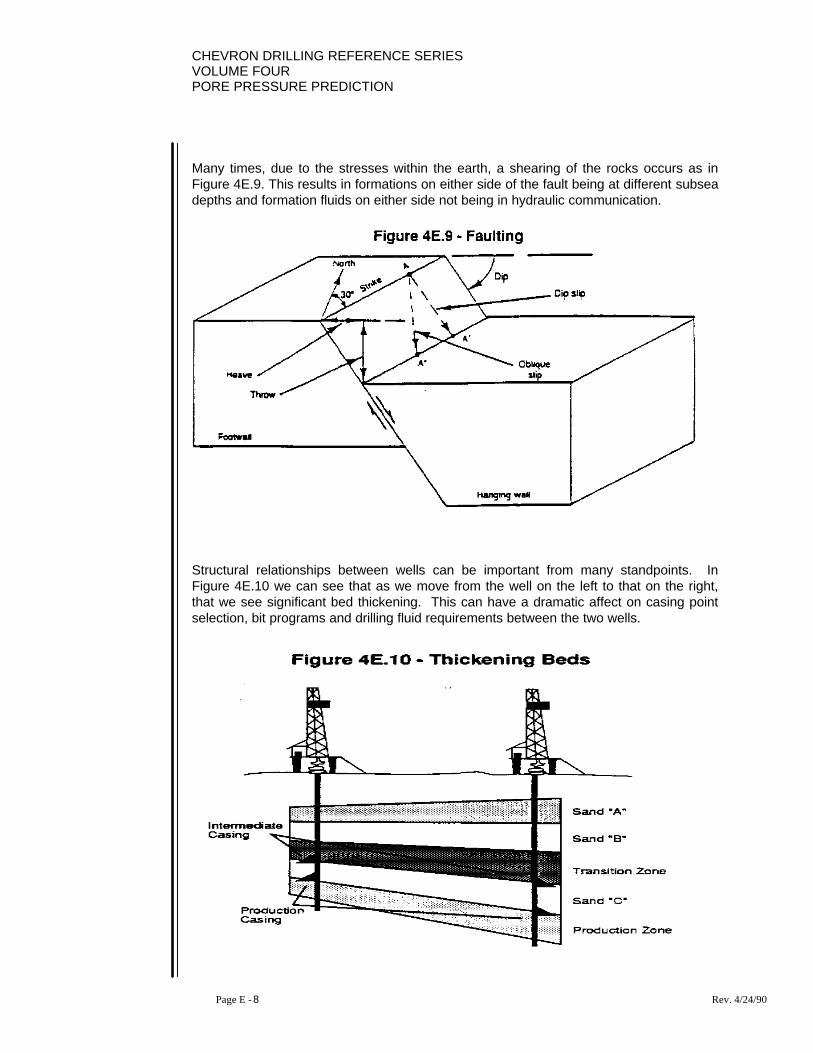
CHEVRON DRILLING REFERENCE SERIESVOLUME FOURPORE PRESSURE PREDICTION
Page E - 8 Rev. 4/24/90
Many times, due to the stresses within the earth, a shearing of the rocks occurs as inFigure 4E.9. This results in formations on either side of the fault being at different subseadepths and formation fluids on either side not being in hydraulic communication.
Structural relationships between wells can be important from many standpoints. InFigure 4E.10 we can see that as we move from the well on the left to that on the right,that we see significant bed thickening. This can have a dramatic affect on casing pointselection, bit programs and drilling fluid requirements between the two wells.

CHEVRON DRILLING REFERENCE SERIESVOLUME FOUR
PORE PRESSURE PREDICTION
Page E - 9 Rev. 4/24/90
Figure 4E.11 is a seismic section which also illustrates the same information as theprevious illustration in the bed thickening. Seismic lines tying proposed wells to anyoffsets provide the drilling man with tremendous information in anticipating formation topsand relative changes in stratigraphy between wells.
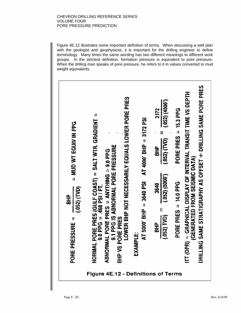
CHEVRON DRILLING REFERENCE SERIESVOLUME FOURPORE PRESSURE PREDICTION
Page E - 10 Rev. 4/24/90
Figure 4E.12 illustrates some important definition of terms. When discussing a well planwith the geologist and geophysicist, it is important for the drilling engineer to defineterminology. Many times the same wording has two different meanings to different workgroups. In the strictest definition, formation pressure is equivalent to pore pressure.When the drilling man speaks of pore pressure, he refers to it in values converted to mudweight equivalents.

CHEVRON DRILLING REFERENCE SERIESVOLUME FOUR
PORE PRESSURE PREDICTION
Page E - 11 Rev. 4/24/90
Normal pore pressure, generally speaking, is equivalent to the native fluid gradient in thearea. Strictly speaking, abnormal pressure is anything but normal, however, the drillingman refers to anything above normal as abnormal, anything below as subnormal.Because we speak of pressures in mud weight equivalents, lower bottom hole pressuredoes not equate to lower pore pressures, and for this reason, drilling the samestratigraphy as an offset does not equate to drilling the same pore pressures. ITT curvesare tools generated from surface seismic data. They are essentially synthetic sonic logsused to predict pore pressures.
Figure 4E.13 illustrates the effect dipping beds have on pore pressure in normallypressured environments, in that there is no change.

CHEVRON DRILLING REFERENCE SERIESVOLUME FOURPORE PRESSURE PREDICTION
Page E - 12 Rev. 4/24/90
Figure 4E.14 illustrates the effect hydrocarbons have on increasing pore pressure as wemove up dip. Note that the bottom hole pressure is lower but the pore pressure is higherin mud weight equivalent up dip.

CHEVRON DRILLING REFERENCE SERIESVOLUME FOUR
PORE PRESSURE PREDICTION
Page E - 13 Rev. 4/24/90
When in abnormally pressured environments, moving up dip results in higher porepressures in mud weight equivalents as illustrated in Figure 4E.15.

CHEVRON DRILLING REFERENCE SERIESVOLUME FOURPORE PRESSURE PREDICTION
Page E - 14 Rev. 4/24/90
The higher the pore pressure environment, the greater the increase in pore pressureseen as we move up dip as illustrated in Figure 4E.16.
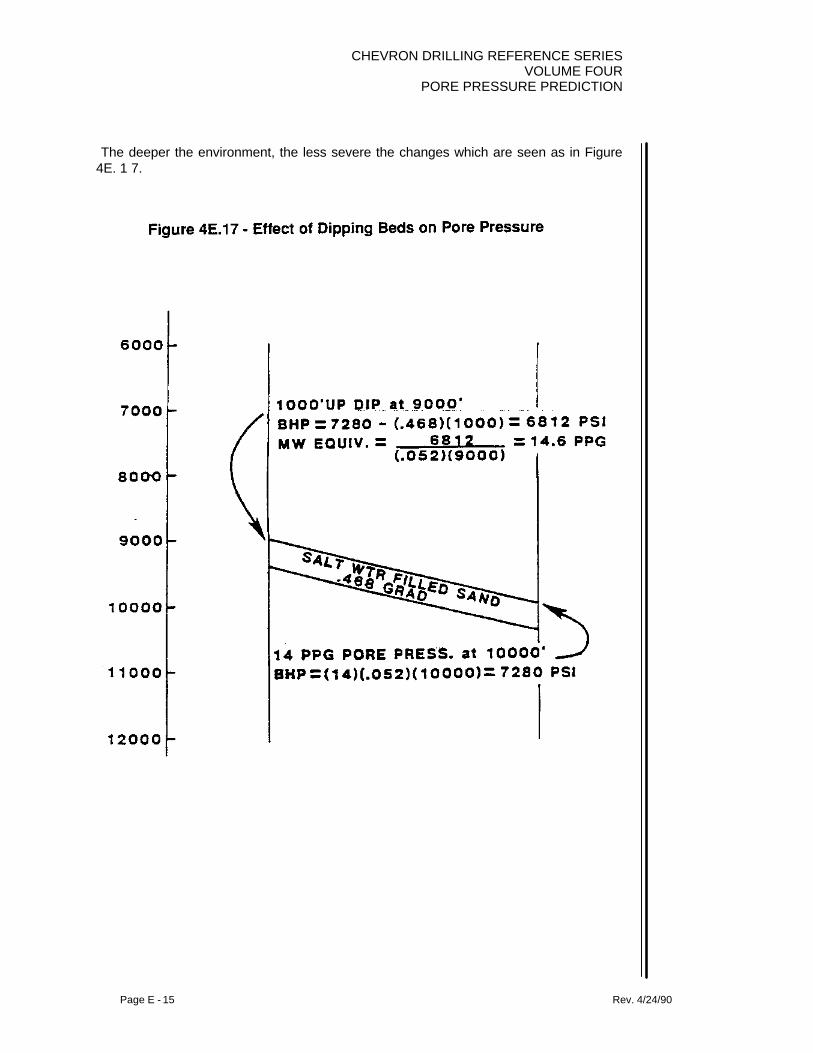
CHEVRON DRILLING REFERENCE SERIESVOLUME FOUR
PORE PRESSURE PREDICTION
Page E - 15 Rev. 4/24/90
The deeper the environment, the less severe the changes which are seen as in Figure4E. 1 7.

CHEVRON DRILLING REFERENCE SERIESVOLUME FOURPORE PRESSURE PREDICTION
Page E - 16 Rev. 4/24/90
Figure 4E.18 summarizes the effects dipping beds have on pore pressures to be seen.
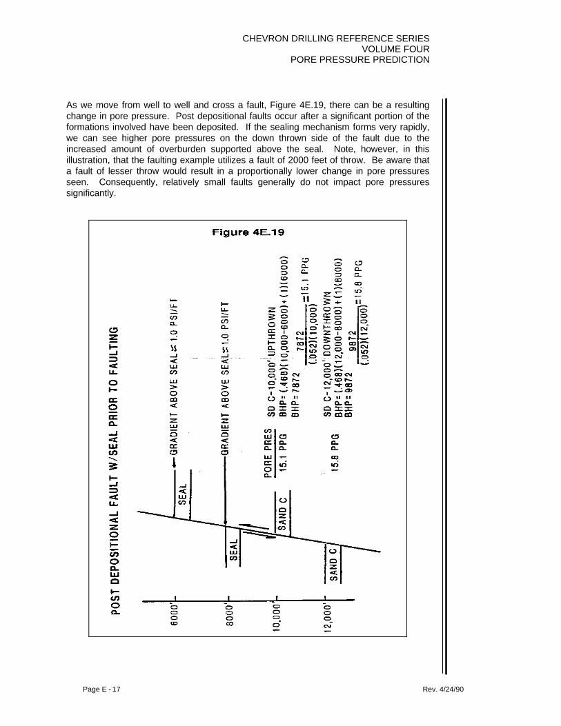
CHEVRON DRILLING REFERENCE SERIESVOLUME FOUR
PORE PRESSURE PREDICTION
Page E - 17 Rev. 4/24/90
As we move from well to well and cross a fault, Figure 4E.19, there can be a resultingchange in pore pressure. Post depositional faults occur after a significant portion of theformations involved have been deposited. If the sealing mechanism forms very rapidly,we can see higher pore pressures on the down thrown side of the fault due to theincreased amount of overburden supported above the seal. Note, however, in thisillustration, that the faulting example utilizes a fault of 2000 feet of throw. Be aware thata fault of lesser throw would result in a proportionally lower change in pore pressuresseen. Consequently, relatively small faults generally do not impact pore pressuressignificantly.

CHEVRON DRILLING REFERENCE SERIESVOLUME FOURPORE PRESSURE PREDICTION
Page E - 18 Rev. 4/24/90
If the sealing mechanism forms very slowly with respect to geological time, as in Figure4E.20, which is the more likely case, the opposite may be true in that the up-thrown sideis the higher pore pressure. This results from the greater overburden load on the down-thrown side causing greater fluid volumes to be squeezed up and out through this slowlydeveloping seal.

CHEVRON DRILLING REFERENCE SERIESVOLUME FOUR
PORE PRESSURE PREDICTION
Page E - 19 Rev. 4/24/90
Depositional faults are those developing gradually along with the deposition which istaking place as in Figure 4E.21. It the sealing mechanism forms very rapidly, with respectto geological time, a similar result is seen in that the down thrown side of the fault can bethe higher pore pressure.

CHEVRON DRILLING REFERENCE SERIESVOLUME FOURPORE PRESSURE PREDICTION
Page E - 20 Rev. 4/24/90
Again with depositional faults, as with post depositional, if the seal formed gradually, theup thrown side can be the higher pore pressure as well, the more likely case, as in Figure4E.22.
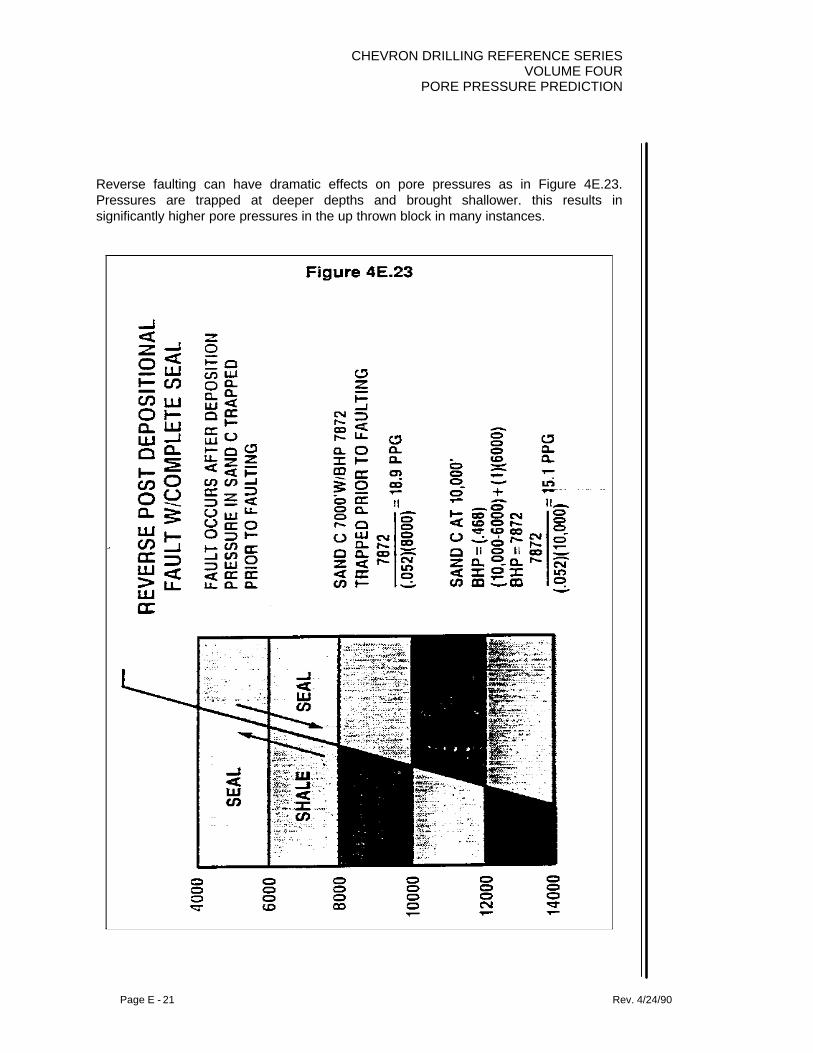
CHEVRON DRILLING REFERENCE SERIESVOLUME FOUR
PORE PRESSURE PREDICTION
Page E - 21 Rev. 4/24/90
Reverse faulting can have dramatic effects on pore pressures as in Figure 4E.23.Pressures are trapped at deeper depths and brought shallower. this results insignificantly higher pore pressures in the up thrown block in many instances.
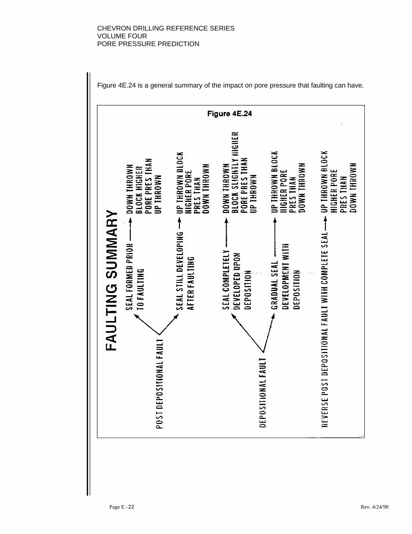
CHEVRON DRILLING REFERENCE SERIESVOLUME FOURPORE PRESSURE PREDICTION
Page E - 22 Rev. 4/24/90
Figure 4E.24 is a general summary of the impact on pore pressure that faulting can have.
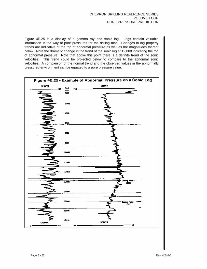
CHEVRON DRILLING REFERENCE SERIESVOLUME FOUR
PORE PRESSURE PREDICTION
Page E - 23 Rev. 4/24/90
Figure 4E.25 is a display of a gamma ray and sonic log. Logs contain valuableinformation in the way of pore pressures for the drilling man. Changes in log propertytrends are indicative of the top of abnormal pressure as well as the magnitudes thereofbelow. Note the dramatic change in the trend of the sonic log at 12,800 indicating the topof abnormal pressure. Note that above this point there is a definite trend of the sonicvelocities. This trend could be projected below to compare to the abnormal sonicvelocities. A comparison of the normal trend and the observed values in the abnormallypressured environment can be equated to a pore pressure value.

CHEVRON DRILLING REFERENCE SERIESVOLUME FOURPORE PRESSURE PREDICTION
Page E - 24 Rev. 4/24/90
Illustrated in Figure 4E.26 are the equations used to compare the normal trends of a logproperty in the normally pressured, normally compacted section of the hole, extrapolateddown, to the observed readings in the abnormally pressured section of the hole.

CHEVRON DRILLING REFERENCE SERIESVOLUME FOUR
PORE PRESSURE PREDICTION
Page E - 25 Rev. 4/24/90

CHEVRON DRILLING REFERENCE SERIESVOLUME FOURPORE PRESSURE PREDICTION
Page E - 26 Rev. 4/24/90
From the pore pressure equations, a pore pressure overlay can be created to determinepore pressures. Figure 4E.27 is such an overlay for resistivity.

CHEVRON DRILLING REFERENCE SERIESVOLUME FOUR
PORE PRESSURE PREDICTION
Page E - 27 Rev. 4/24/90
A pore pressure overlay is applied to the data by aligning the normal trend line of theoverlay through the data points of the normally pressured normally compacted section ofthe hole as in Figure 4E.28. Values of abnormal pressure are then read directly from theoverlay in the sections below.

CHEVRON DRILLING REFERENCE SERIESVOLUME FOURPORE PRESSURE PREDICTION
Page E - 28 Rev. 4/24/90
Pore pressures are determined in offset wells and projected to a proposed location forwell planning. In the seismic illustration of Figure 4E.29 we evaluate the pore pressuresseen in the down dip well in the center of the seismic trace. We are concerned with whatto expect in the updip wellbores proposed to the left. We will look at the updip directionalwell to illustrate how this works.

CHEVRON DRILLING REFERENCE SERIESVOLUME FOUR
PORE PRESSURE PREDICTION
Page E - 29 Rev. 4/24/90
If we merely designed this up dip well to utilize the casing program which was seen to beadequate in the down dip well, then the casing program proposed would be that on theleft of Figure 4E.30. However, due to the encountering of all stratigraphies significantlyup dip, we would find ourselves stopping short of the same stratigraphic horizon achievedin the offset and would actual see the scenario on the left occur. Let’s examine why?
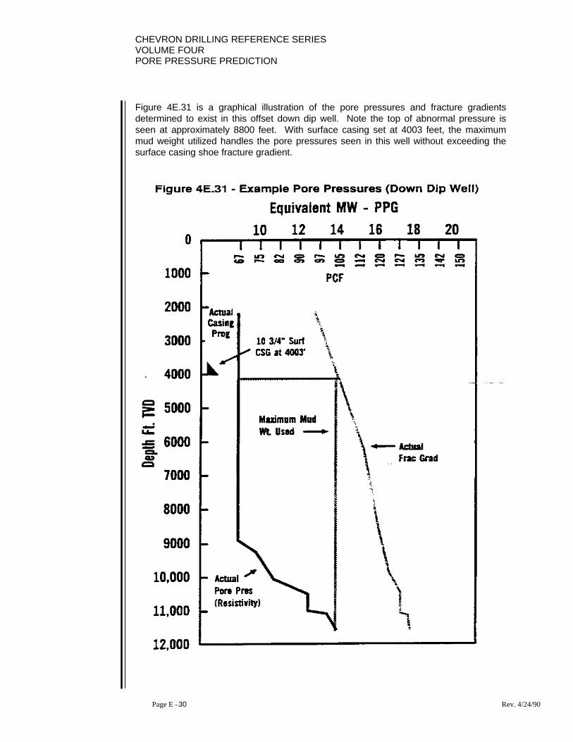
CHEVRON DRILLING REFERENCE SERIESVOLUME FOURPORE PRESSURE PREDICTION
Page E - 30 Rev. 4/24/90
Figure 4E.31 is a graphical illustration of the pore pressures and fracture gradientsdetermined to exist in this offset down dip well. Note the top of abnormal pressure isseen at approximately 8800 feet. With surface casing set at 4003 feet, the maximummud weight utilized handles the pore pressures seen in this well without exceeding thesurface casing shoe fracture gradient.

CHEVRON DRILLING REFERENCE SERIESVOLUME FOUR
PORE PRESSURE PREDICTION
Page E - 31 Rev. 4/24/90
However, in the proposed well, we will be encountering formations significantly up dip.Projecting these we find that the transition zone will be seen approximately 2000 feet updip as in Figure 4E.32. When we estimate all the pore pressures for the formations to beseen in their new up dip position they will all be higher in magnitude. If we set surfacecasing even deeper than in the offset well at 4589 feet, we find we cannot reachauthorized depth without another string of casing without infringing on our surface casingshoe integrity.
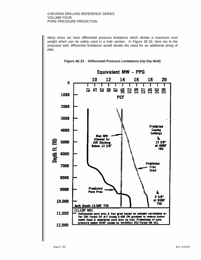
CHEVRON DRILLING REFERENCE SERIESVOLUME FOURPORE PRESSURE PREDICTION
Page E - 32 Rev. 4/24/90
Many times we have differential pressure limitations which dictate a maximum mudweight which can be safely used in a hole section. In Figure 4E.33, here too in theproposed well, differential limitations would dictate the need for an additional string ofpipe.
Figure 4E.33 - Differential Pressure Limitations (Up Dip Well)
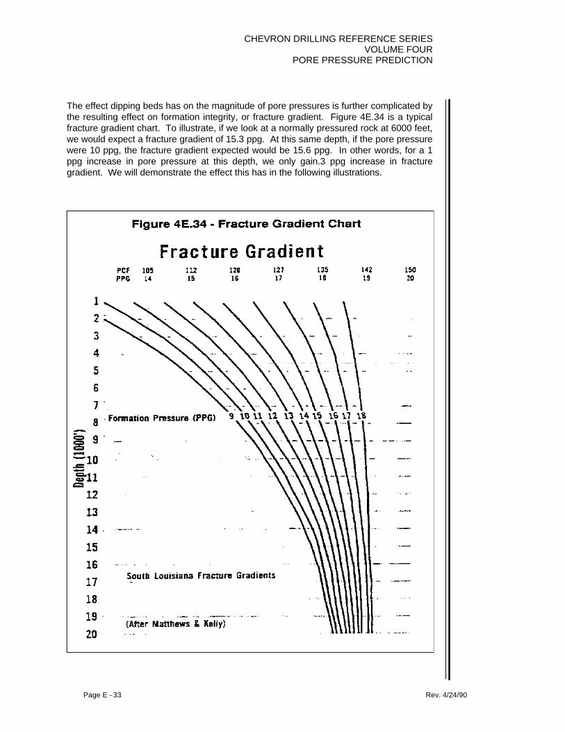
CHEVRON DRILLING REFERENCE SERIESVOLUME FOUR
PORE PRESSURE PREDICTION
Page E - 33 Rev. 4/24/90
The effect dipping beds has on the magnitude of pore pressures is further complicated bythe resulting effect on formation integrity, or fracture gradient. Figure 4E.34 is a typicalfracture gradient chart. To illustrate, if we look at a normally pressured rock at 6000 feet,we would expect a fracture gradient of 15.3 ppg. At this same depth, if the pore pressurewere 10 ppg, the fracture gradient expected would be 15.6 ppg. In other words, for a 1ppg increase in pore pressure at this depth, we only gain.3 ppg increase in fracturegradient. We will demonstrate the effect this has in the following illustrations.

CHEVRON DRILLING REFERENCE SERIESVOLUME FOURPORE PRESSURE PREDICTION
Page E - 34 Rev. 4/24/90
Consider the case of an existing offset well and a proposed well located slightly up dip.Figure 4E.35 is a graphical display of the pore pressures and fracture gradientsdetermined to exist in the off set well. Note the top of abnormal pressure is atapproximately 5500 feet.

CHEVRON DRILLING REFERENCE SERIESVOLUME FOUR
PORE PRESSURE PREDICTION
Page E - 35 Rev. 4/24/90
As we determine the depths at which we will encounter the horizons in the proposed welland estimate pore pressures to be seen, we find the top of pressure will be up dip atapproximately 4800 feet as in Figure 4E.36.

CHEVRON DRILLING REFERENCE SERIESVOLUME FOURPORE PRESSURE PREDICTION
Page E - 36 Rev. 4/24/90
Illustrating the impact on fracture gradient, we see that for significant increases in porepressures, small increases in expected fracture gradient result as in Figure 4E.37. Thisresults in a narrower band of limits between which we have to select casing points.

CHEVRON DRILLING REFERENCE SERIESVOLUME FOUR
PORE PRESSURE PREDICTION
Page E - 37 Rev. 4/24/90
Once a prediction or pore pressures and fracture gradients is made, we can thendetermine, as far as pressures are concerned, casing points. For instance, in Figure4E.38 we can see that a minimum of 3200 feet of surface casing is required in order toreach a depth of 5500 feet.

CHEVRON DRILLING REFERENCE SERIESVOLUME FOURPORE PRESSURE PREDICTION
Page E - 38 Rev. 4/24/90
In Figure 4E.39, we see that if we chose to set surface casing at an arbitrary depth of3370 feet, then two strings of intermediate casing would be required to reach a depth of10,000 feet.,

CHEVRON DRILLING REFERENCE SERIESVOLUME FOUR
PORE PRESSURE PREDICTION
Page E - 39 Rev. 4/24/90
In Figure 4E.40, we see that if surface casing were set at a depth of 4745 feet, then oneintermediate string of casing would be required to reach a depth of 10,000 feet.

CHEVRON DRILLING REFERENCE SERIESVOLUME FOURPORE PRESSURE PREDICTION
Page E - 40 Rev. 4/24/90
CHEVRON DRILLING REFERENCE SERIESVOLUME FOUR
PORE PRESSURE PREDICTION
Page F - 1 Rev. 4/24/90
SECTION F: ITT INTERPRETATION
1. INTRODUCTION
An accurate prediction of formation pore pressures prior to drilling a well can significantlyimprove drilling performance, reduce the number of costly drilling problems encountered,and in many instances, can be the determining factor in successfully reaching objectives.This is particularly true when dealing with exploratory wells. The fact that we are going topenetrate the same stratigraphies as offset wells does not equate to being in the samepore pressure environment. In fact, when dealing with exploratory wells, there is a highpercentage of the time when this is not the case.
This approach to predicting formation pore pressures utilizes offset log information, andvelocity information from surface seismic data. All surface seismic data has velocityinformation built into ft in the way of stacking velocities. From these stacking velocities,estimates of interval velocities can be made. We have developed a quantitativetechnique for determining formation pore pressures from the relative changes in thesevelocities.
From the stacking velocity data, we develop curves we refer to as ITT (Interval TransitTime) curves. ITT curves are generated at offset locations as well as the proposeddrilling location. Actual offset well pore pressures are determined from the logs and theITT curves at these offsets are calibrated to the known pressures. After this calibrationprocess, the ITT at the proposed location can be interpreted to predict formation porepressures to be encountered.
The combination of these tools yields a reliable pore pressure scenario from which toplan a drilling program and execute the operations. This procedure has been utilized onnumerous wells throughout the Gulf of Mexico as well as a number of wells around theworld. The technique will be illustrated with Figures 4F.1 through 4F.14 as a step by stepanalysis is done. Results of the use of this methodology will also be illustrated.
2. BACKGROUND
A Mr. Pennebaker did some research back in the sixties on interval velocities vs. depthfor various geological ages in normally pressured environments. The results of his workindicate trends which appear to be straight lines on a log-log scale (see Figure 4F.1below).

CHEVRON DRILLING REFERENCE SERIESVOLUME FOURPORE PRESSURE PREDICTION
Page F - 2 Rev. 4/24/90

CHEVRON DRILLING REFERENCE SERIESVOLUME FOUR
PORE PRESSURE PREDICTION
Page F - 3 Rev. 4/24/90
If we take one of these curves, such as that for the Pliocene age, and re-plot the data ona semi-logarithmic scale, with the vertical linear scale for depth in feet, and the horizontallog scale for interval velocity in microseconds per foot, we obtain a curve like the one inFigure 4F.2. This indicates a curved relationship with respect to depth for interval velocityin a normally pressured, homogeneous environment.

CHEVRON DRILLING REFERENCE SERIESVOLUME FOURPORE PRESSURE PREDICTION
Page F - 4 Rev. 4/24/90
Procedure
ITT curves are generated at the offset wells as in Figure 4F.3. Lithology tops areindicated with respect to the ITT curve based on where they are seen on the gamma raysonic log. Keep in mind that slight differences in the depths of these lithologies may existon the ITT vs. the gamma ray sonic, since the velocities in the ITT are not accurateinterval velocities. A comparison of the ITT to the gamma ray sonic log is necessary toselect these lithology tops on the ITT. Some of the less significant velocity shifts acrosslithology tops will be ignored, but the more dramatic ones will be honored.

CHEVRON DRILLING REFERENCE SERIESVOLUME FOUR
PORE PRESSURE PREDICTION
Page F - 5 Rev. 4/24/90
Velocity trend lines are then drawn on the ITT curve within lithological sections. It isimportant to stay on the same velocity side of the ITT curve as was determined to benecessary in the pore pressure determination process while plotting the sonic log of theoffset well. This has been done in Figure 4F.4. Note that only the significant velocityshifts have been honored.

CHEVRON DRILLING REFERENCE SERIESVOLUME FOURPORE PRESSURE PREDICTION
Page F - 6 Rev. 4/24/90
The ITT velocity trend lines are traced within lithological sections. Upon arriving at asignificant velocity shift at a lithology top a recalibration is performed. This is done byshifting the trace and aligning the last velocity value of the trend in the previouslithological section, with the first velocity value of the next. Tracing of the velocity trendline in the next lithological section is then done until a continuous velocity trend profile isobtained. Recalibration of the ITT velocity trends appears in Figure 4F.5.

CHEVRON DRILLING REFERENCE SERIESVOLUME FOUR
PORE PRESSURE PREDICTION
Page F - 7 Rev. 4/24/90
Pore pressures are then determined from the ITT and calibrated to the known porepressures in this offset well. This is done with several possible interpretationapproaches, two of which will be illustrated here. In the first interpretative approach, wetake a typical Pennebaker curve such as the one in Figure 4F.2, and align it against theITT curve to identify the normally pressured, normally compacted interval as in Figure4F.6. The ITT curve departs from this Pennebaker curve at approximately 5300 feet.

CHEVRON DRILLING REFERENCE SERIESVOLUME FOURPORE PRESSURE PREDICTION
Page F - 8 Rev. 4/24/90
We then take the recalibrated velocity trend line curve of Figure 4F.5, and draw a straightnormal trend line through the velocity trend down to this depth of 5300 feet. We thencreate a pore pressure overlay for use on ITT curves in the area. We solve for thepressure exponent using a known pressure point in this offset well. As in Figure 4F.7, wethen, at the same depth of this known pore pressure point, assume pore pressures inincrements of 1 ppg, and solve for observed values of interval transit time. Throughthese observed values of interval transit time, parallel trend lines are drawn to the normaltrend line previously selected.
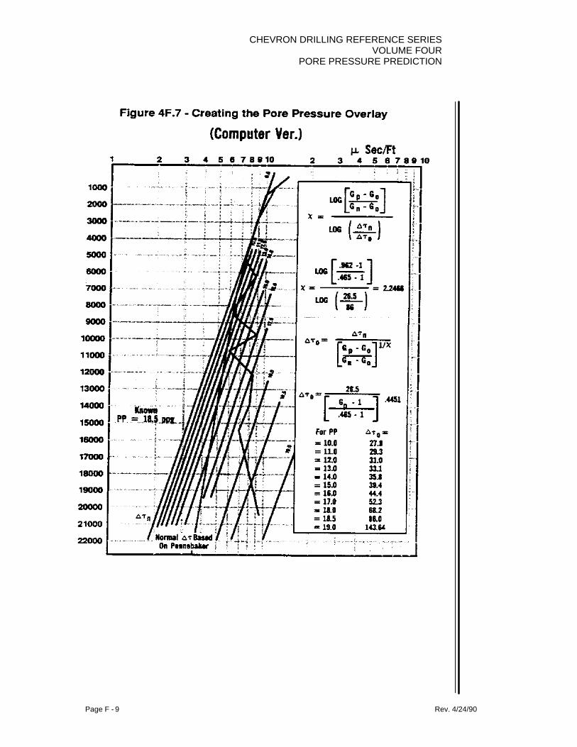
CHEVRON DRILLING REFERENCE SERIESVOLUME FOUR
PORE PRESSURE PREDICTION
Page F - 9 Rev. 4/24/90

CHEVRON DRILLING REFERENCE SERIESVOLUME FOURPORE PRESSURE PREDICTION
Page F - 10 Rev. 4/24/90
A comparison of pore pressures determined from the ITT and the mud weights used onthis offset well appear in Figure 4F.8.

CHEVRON DRILLING REFERENCE SERIESVOLUME FOUR
PORE PRESSURE PREDICTION
Page F - 11 Rev. 4/24/90
Note, between the depths of 5300 and 8800, that the ITT is reacting to the porosity seenin this interval, Figure 4F.9, and not to pressure. Lithological information such as thisneeds always to be kept in mind during the interpretation process.

CHEVRON DRILLING REFERENCE SERIESVOLUME FOURPORE PRESSURE PREDICTION
Page F - 12 Rev. 4/24/90
An alternate approach is illustrated in Figure 4F.10. Here, a normal velocity trend line isdrawn through the apparent normally pressured, normally compacted intervalimmediately above the top of pressure as determined from plotting the sonic log on thiswell. The same procedure of solving for the pressure exponent, and creating an overlayfor the ITT as before is followed.

CHEVRON DRILLING REFERENCE SERIESVOLUME FOUR
PORE PRESSURE PREDICTION
Page F - 13 Rev. 4/24/90
A comparison of pore pressures from the ITT utilizing this approach, and the mudweights used to drill this well appear in Figure 4F.11.

CHEVRON DRILLING REFERENCE SERIESVOLUME FOURPORE PRESSURE PREDICTION
Page F - 14 Rev. 4/24/90
To insure a quality ITT pore pressure overlay has been created, and proper solution ofthe pressure exponent, the overlay should be used on the ITT of another offset well. InFigure 4F.12, we have an ITT on another offset well with velocity trend lines selected.

CHEVRON DRILLING REFERENCE SERIESVOLUME FOUR
PORE PRESSURE PREDICTION
Page F - 15 Rev. 4/24/90
Application of the overlay, developed from the second approach, to the recalibratedvelocity trend lines appears in Figure 4F.13.
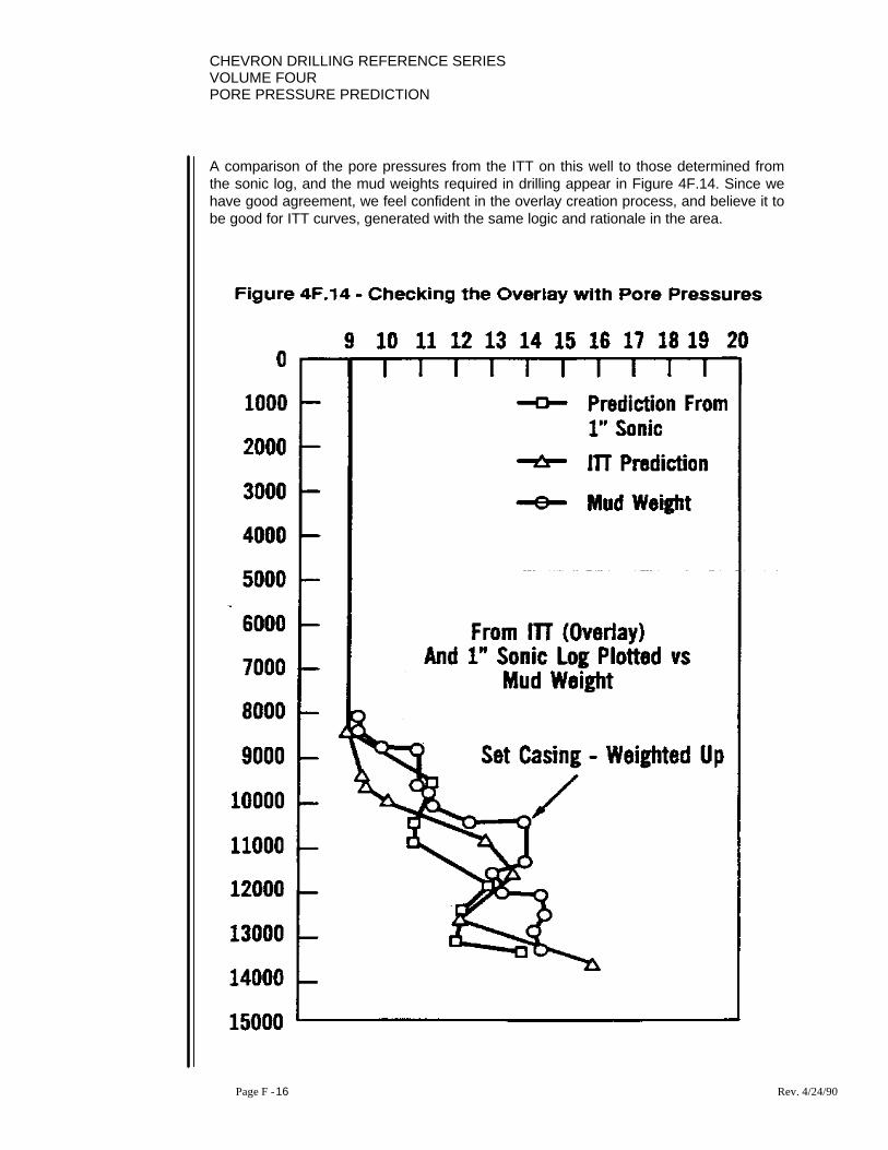
CHEVRON DRILLING REFERENCE SERIESVOLUME FOURPORE PRESSURE PREDICTION
Page F - 16 Rev. 4/24/90
A comparison of the pore pressures from the ITT on this well to those determined fromthe sonic log, and the mud weights required in drilling appear in Figure 4F.14. Since wehave good agreement, we feel confident in the overlay creation process, and believe it tobe good for ITT curves, generated with the same logic and rationale in the area.

CHEVRON DRILLING REFERENCE SERIESVOLUME FOUR
PORE PRESSURE PREDICTION
Page F - 17 Rev. 4/24/90
An ITT is generated at the proposed location and lithological tops which dictate arecalibration in velocity trends are correlated through seismic ties and indicated as inFigure 4F.15.

CHEVRON DRILLING REFERENCE SERIESVOLUME FOURPORE PRESSURE PREDICTION
Page F - 18 Rev. 4/24/90
ITT velocity trends are determined as before in Figure 4F.16.

CHEVRON DRILLING REFERENCE SERIESVOLUME FOUR
PORE PRESSURE PREDICTION
Page F - 19 Rev. 4/24/90
The velocity trends are recalibrated into a continuous curve as in Figure 4F.17.
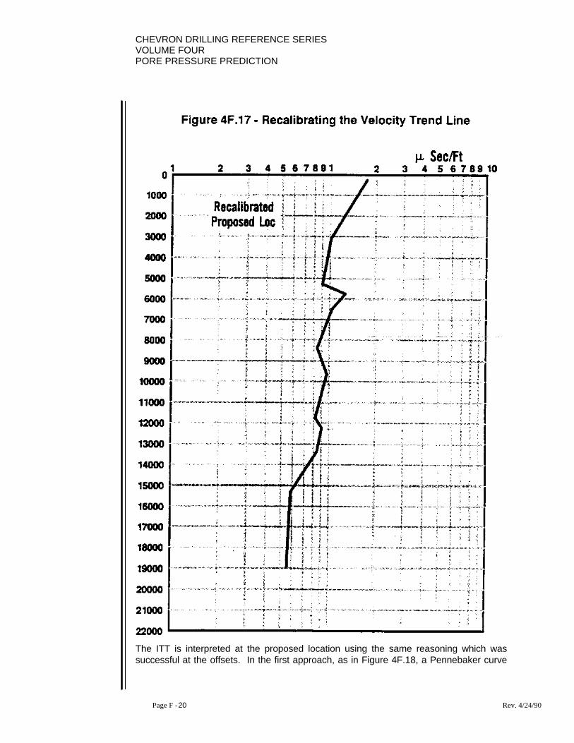
CHEVRON DRILLING REFERENCE SERIESVOLUME FOURPORE PRESSURE PREDICTION
Page F - 20 Rev. 4/24/90
The ITT is interpreted at the proposed location using the same reasoning which wassuccessful at the offsets. In the first approach, as in Figure 4F.18, a Pennebaker curve

CHEVRON DRILLING REFERENCE SERIESVOLUME FOUR
PORE PRESSURE PREDICTION
Page F - 21 Rev. 4/24/90
is aligned with the ITT curve at the proposed well. identifying the normally pressurednormally compacted section.

CHEVRON DRILLING REFERENCE SERIESVOLUME FOURPORE PRESSURE PREDICTION
Page F - 22 Rev. 4/24/90
Again a straight normal trend line is drawn through the velocity trend in this interval. TheITT pore pressure overlay created in this approach is used on the recalibrated velocitytrends as in Figure 4F.19.
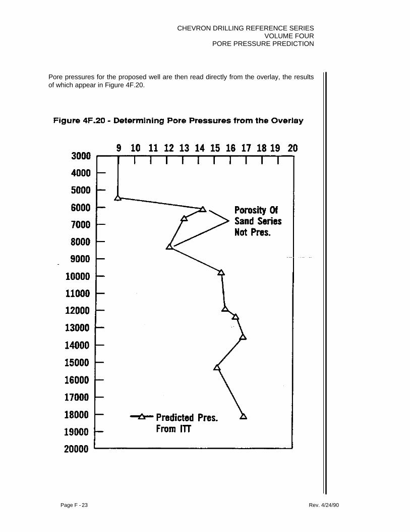
CHEVRON DRILLING REFERENCE SERIESVOLUME FOUR
PORE PRESSURE PREDICTION
Page F - 23 Rev. 4/24/90
Pore pressures for the proposed well are then read directly from the overlay, the resultsof which appear in Figure 4F.20.
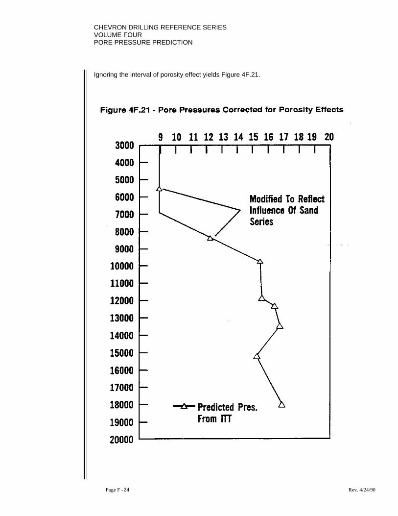
CHEVRON DRILLING REFERENCE SERIESVOLUME FOURPORE PRESSURE PREDICTION
Page F - 24 Rev. 4/24/90
Ignoring the interval of porosity effect yields Figure 4F.21.
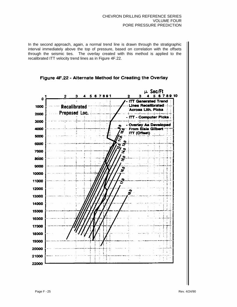
CHEVRON DRILLING REFERENCE SERIESVOLUME FOUR
PORE PRESSURE PREDICTION
Page F - 25 Rev. 4/24/90
In the second approach, again, a normal trend line is drawn through the stratigraphicinterval immediately above the top of pressure, based on correlation with the offsetsthrough the seismic ties. The overlay created with this method is applied to therecalibrated ITT velocity trend lines as in Figure 4F.22.
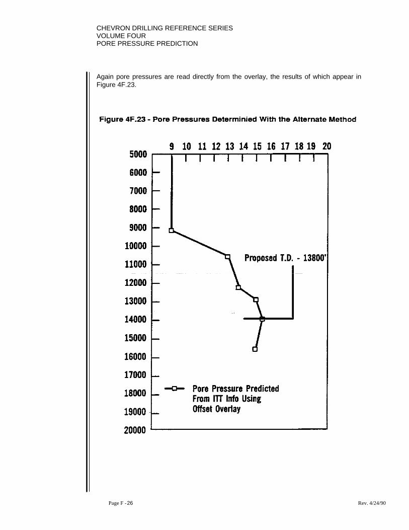
CHEVRON DRILLING REFERENCE SERIESVOLUME FOURPORE PRESSURE PREDICTION
Page F - 26 Rev. 4/24/90
Again pore pressures are read directly from the overlay, the results of which appear inFigure 4F.23.

CHEVRON DRILLING REFERENCE SERIESVOLUME FOUR
PORE PRESSURE PREDICTION
Page F - 27 Rev. 4/24/90
REFERENCES
1. E. S. Pennebaker, An Engineering Interpretation of Seismic Data, SPE paper2165.

CHEVRON DRILLING REFERENCE SERIESVOLUME FOURPORE PRESSURE PREDICTION
Page F - 28 Rev. 4/24/90

CHEVRON DRILLING REFERENCE SERIESVOLUME FOURPORE PRESSURE PREDICTION
Page G - 1 Rev. 4/24/96
SECTION G: ITT CARBONATES
1. INTRODUCTION
M I S S I N G

CHEVRON DRILLING REFERENCE SERIESVOLUME FOUR
PORE PRESSURE PREDICTION
Page H - 1 Rev. 4/24/90
SECTION H: ITT INTERPRETATION, AN ALTERNATEAPPROACH FOR GULF COAST WELLS
1. INTRODUCTION
All surface seismic data has velocity information built into it in the way of stackingvelocities. From these stacking velocities, estimates of interval velocities can bedetermined. We have developed a quantitative technique for determining formation porepressures from the relative changes in these velocities.
From the stacking velocity data, we develop curves which we refer to as ITT (IntervalTransit Time) curves. The ITT curves are generated at the proposed location and arecorrelated to offset location curves to calibrate velocities. Offset location pore pressuresare predicted and are combined with structural geology to predict anticipated porepressures of the proposed wellbore. With these curves, in conjunction with geologicalinformation to determine structural changes, and offset logs to determine pore pressuresin offsets, we can predict pore pressures to be encountered in a proposed wellbore.
To date, we have made such predictions of pore pressure in approximately 20exploratory wells on the Gulf Coast prior to their drilling, with excellent results. We willgraphically show results on a number of these wells comparing both the mud weightsrequired, as dictated by hole conditions, and the actual pore pressures encountered. Ourstatistics within Chevron, on the Gulf Coast, indicate that proposed casing programs areadequate for the needs of an exploratory well:
29% of the time if offset casing programs are used,
65% of the time if detailed geological information is used,
>95% of the time if ITT data is also incorporated.
Significant dollars can be saved and increased success in reaching objectives can berealized when pore pressures can be anticipated prior to drilling a well. This techniqueoffers the opportunity to do so.
Accurately predicting formation pore pressures in advance on exploratory wells hasalways been an industry problem. Where abnormal pore pressures are encountered,casing point selection becomes critical to the successful drilling of the well, and it porepressures are not accurately defined prior to drilling, casing programs are many timesinadequate or are over designed. This can lead to wells which are unsuccessful atreaching objectives or are too costly or both.

CHEVRON DRILLING REFERENCE SERIESVOLUME FOURPORE PRESSURE PREDICTION
Page H - 2 Rev. 4/24/90
We have developed techniques whereby surface seismic data can be utilized to aid in theprediction of formation pore pressures prior to the drilling of a well. Although thesetechniques have been developed for many drilling environments, this technique focuseson the sand shale depositional environment.
2. BACKGROUND INFORMATION
Since seismic information has velocity information built into the data by the very nature ofhow it is recorded, in the process of stacking the data, stacking velocities are determined.From these velocities, interval velocities can be determined. Since all seismicinformation contains this velocity information, all geophysical companies have thecapability to generate a curve of interval velocity vs. depth at any point on a seismic line.This, essentially, becomes a synthetic sonic log. Mr. Pennebaker (1) did some researchback in the sixties on interval velocities vs. depth for various geological ages in normallypressured environments. The results of his work appears in Figure 4H.1.

CHEVRON DRILLING REFERENCE SERIESVOLUME FOUR
PORE PRESSURE PREDICTION
Page H - 3 Rev. 4/24/90
Since the trends appear to be straight lines on this log-log scale, we merely extrapolatedthe data to deeper depths as in Figure 4H.2. If we take one of these curves, such as thatfor the Pliocene age, and re-plot the data on a semi-logarithmic scale, with the verticallinear scale for depth in feet and the horizontal log scale for interval velocity in microseconds per foot, we obtain a curve like the one in Figure 4H.3, where we observe acurved relationship with respect to depth for interval velocity in a normally pressuredenvironment.
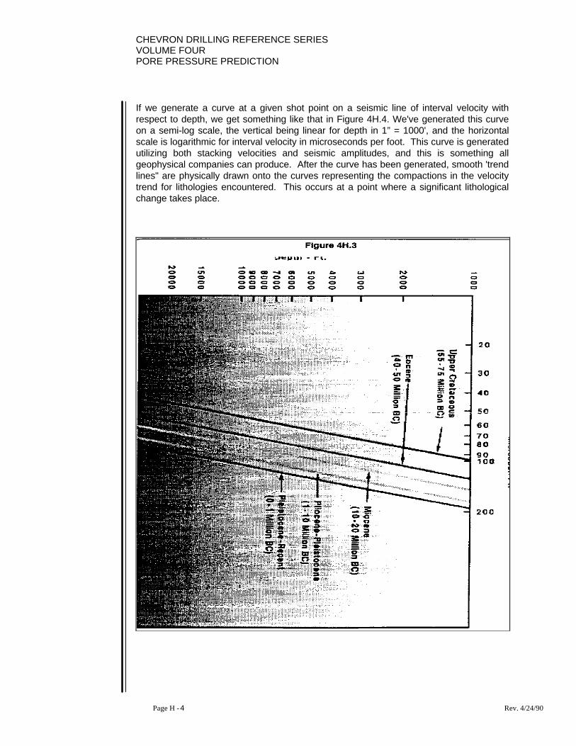
CHEVRON DRILLING REFERENCE SERIESVOLUME FOURPORE PRESSURE PREDICTION
Page H - 4 Rev. 4/24/90
If we generate a curve at a given shot point on a seismic line of interval velocity withrespect to depth, we get something like that in Figure 4H.4. We've generated this curveon a semi-log scale, the vertical being linear for depth in 1” = 1000', and the horizontalscale is logarithmic for interval velocity in microseconds per foot. This curve is generatedutilizing both stacking velocities and seismic amplitudes, and this is something allgeophysical companies can produce. After the curve has been generated, smooth 'trendlines" are physically drawn onto the curves representing the compactions in the velocitytrend for lithologies encountered. This occurs at a point where a significant lithologicalchange takes place.
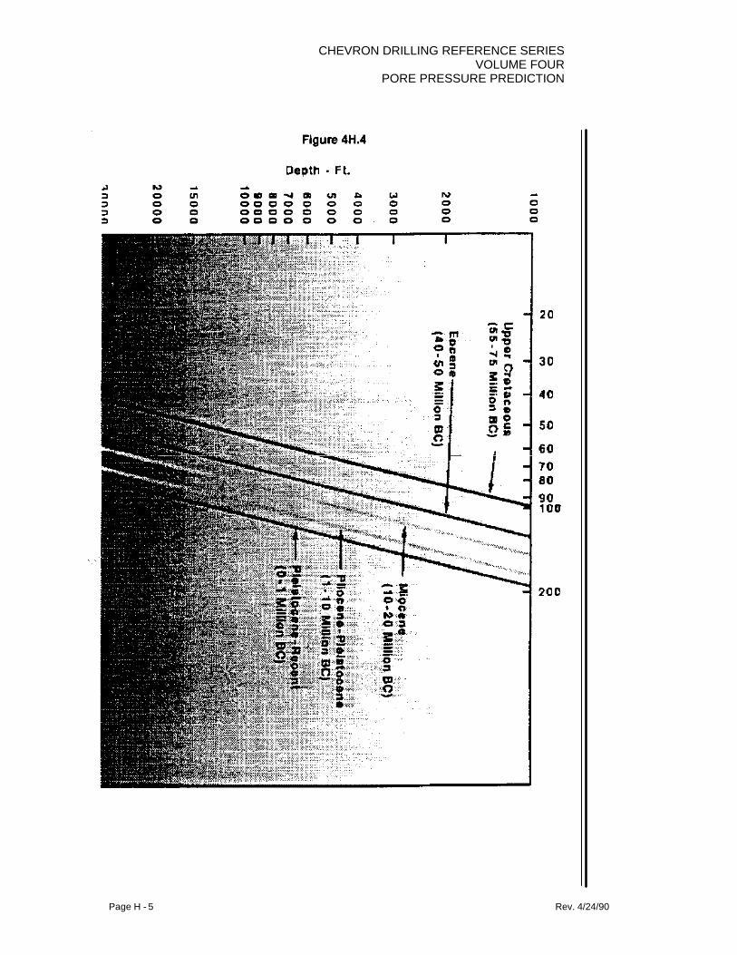
CHEVRON DRILLING REFERENCE SERIESVOLUME FOUR
PORE PRESSURE PREDICTION
Page H - 5 Rev. 4/24/90
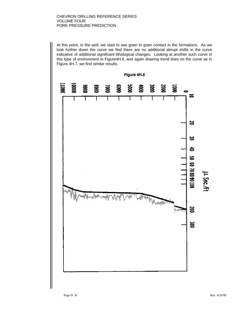
CHEVRON DRILLING REFERENCE SERIESVOLUME FOURPORE PRESSURE PREDICTION
Page H - 6 Rev. 4/24/90
At this point, in the well, we start to see grain to grain contact in the formations. As welook further down the curve we find there are no additional abrupt shifts in the curveindicative of additional significant lithological changes. Looking at another such curve inthis type of environment in Figure4H.6, and again drawing trend lines on the curve as inFigure 4H.7, we find similar results.

CHEVRON DRILLING REFERENCE SERIESVOLUME FOUR
PORE PRESSURE PREDICTION
Page H - 7 Rev. 4/24/90
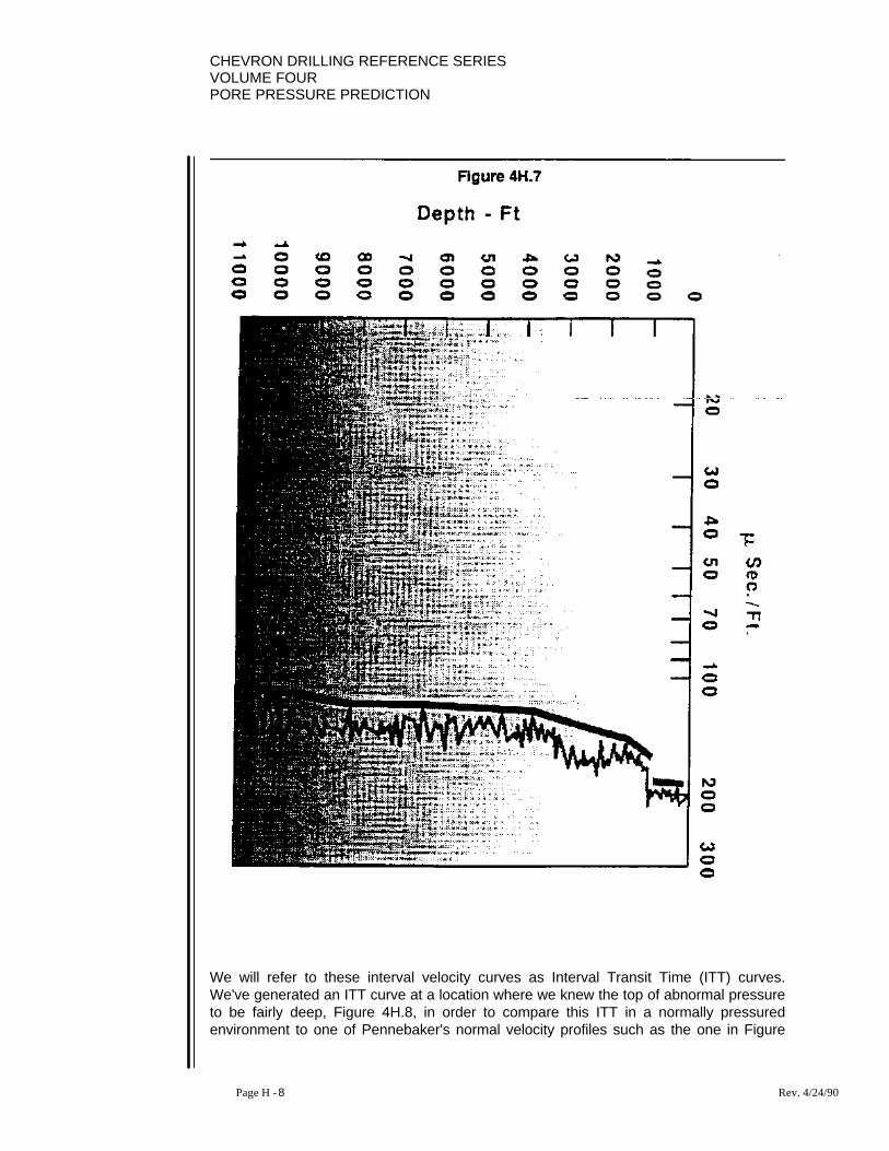
CHEVRON DRILLING REFERENCE SERIESVOLUME FOURPORE PRESSURE PREDICTION
Page H - 8 Rev. 4/24/90
We will refer to these interval velocity curves as Interval Transit Time (ITT) curves.We've generated an ITT curve at a location where we knew the top of abnormal pressureto be fairly deep, Figure 4H.8, in order to compare this ITT in a normally pressuredenvironment to one of Pennebaker's normal velocity profiles such as the one in Figure

CHEVRON DRILLING REFERENCE SERIESVOLUME FOUR
PORE PRESSURE PREDICTION
Page H - 9 Rev. 4/24/90
4H.3. If we compare the velocity trend from Pennebaker in Figure 4H.3 to the curve inFigure 4H.8, but display the Pennebaker information to the left a bit so the two curves donot overlap, we arrive at Figure 4H.9.
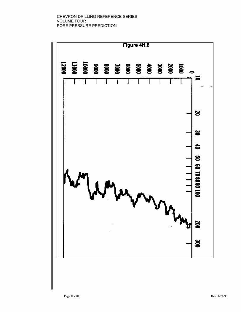
CHEVRON DRILLING REFERENCE SERIESVOLUME FOURPORE PRESSURE PREDICTION
Page H - 10 Rev. 4/24/90
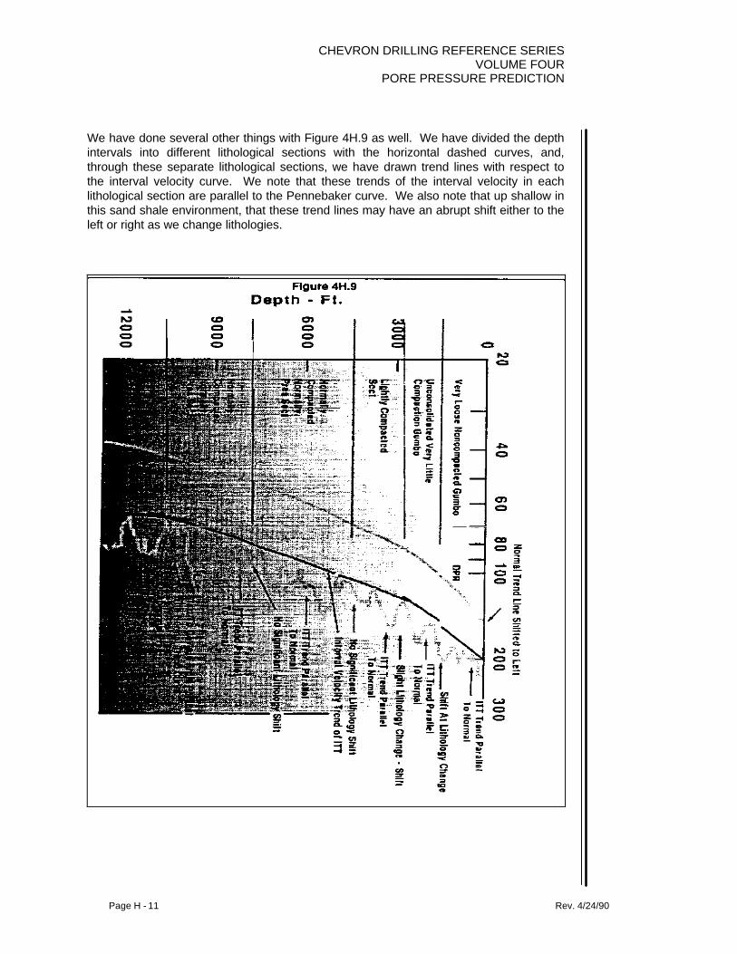
CHEVRON DRILLING REFERENCE SERIESVOLUME FOUR
PORE PRESSURE PREDICTION
Page H - 11 Rev. 4/24/90
We have done several other things with Figure 4H.9 as well. We have divided the depthintervals into different lithological sections with the horizontal dashed curves, and,through these separate lithological sections, we have drawn trend lines with respect tothe interval velocity curve. We note that these trends of the interval velocity in eachlithological section are parallel to the Pennebaker curve. We also note that up shallow inthis sand shale environment, that these trend lines may have an abrupt shift either to theleft or right as we change lithologies.

CHEVRON DRILLING REFERENCE SERIESVOLUME FOURPORE PRESSURE PREDICTION
Page H - 12 Rev. 4/24/90
However, as we go deeper there are no lithological changes which cause these abruptshifts in interval velocity. From many such observations at various locations in sandshale environments, we have concluded that the general shape of the interval velocitycurve is what is curve. We use stacking velocities only, and run a smoothing function onthe data which yields a very smooth ITT curve.
Figures 4H.10 and 4H.11 represent comparisons of “smoothed" ITT curves againstnormal ITT curves. This is a necessary comparison to be sure the data has not beenpoorly manipulated as is illustrated in Figure 4H.12 where the smooth version is in pooragreement with the original.

CHEVRON DRILLING REFERENCE SERIESVOLUME FOUR
PORE PRESSURE PREDICTION
Page H - 13 Rev. 4/24/90

CHEVRON DRILLING REFERENCE SERIESVOLUME FOURPORE PRESSURE PREDICTION
Page H - 14 Rev. 4/24/90

CHEVRON DRILLING REFERENCE SERIESVOLUME FOUR
PORE PRESSURE PREDICTION
Page H - 15 Rev. 4/24/90

CHEVRON DRILLING REFERENCE SERIESVOLUME FOURPORE PRESSURE PREDICTION
Page H - 16 Rev. 4/24/90
3. PROCEDURE
In the pore pressure determination process of an ITT curve, we utilize equationsdeveloped by Mr. Ben Eaton. These equations appear in Figure 4H.13. Morespecifically, we use his equation for interval transit time. Eaton's equations relate porepressures for an interval to a relationship between observed values of a parameter andwhat the normal values would be for a normally pressured formation occurring at thesame depth. His equations also require the values of the overburden stress gradient forthat depth, Figure 4H.14, and the matrix stress coefficient for that same depth, Figure4H.15. Knowing these facts, we are ready to illustrate how we use ITT curves to predictpore pressures at a proposed drilling location.
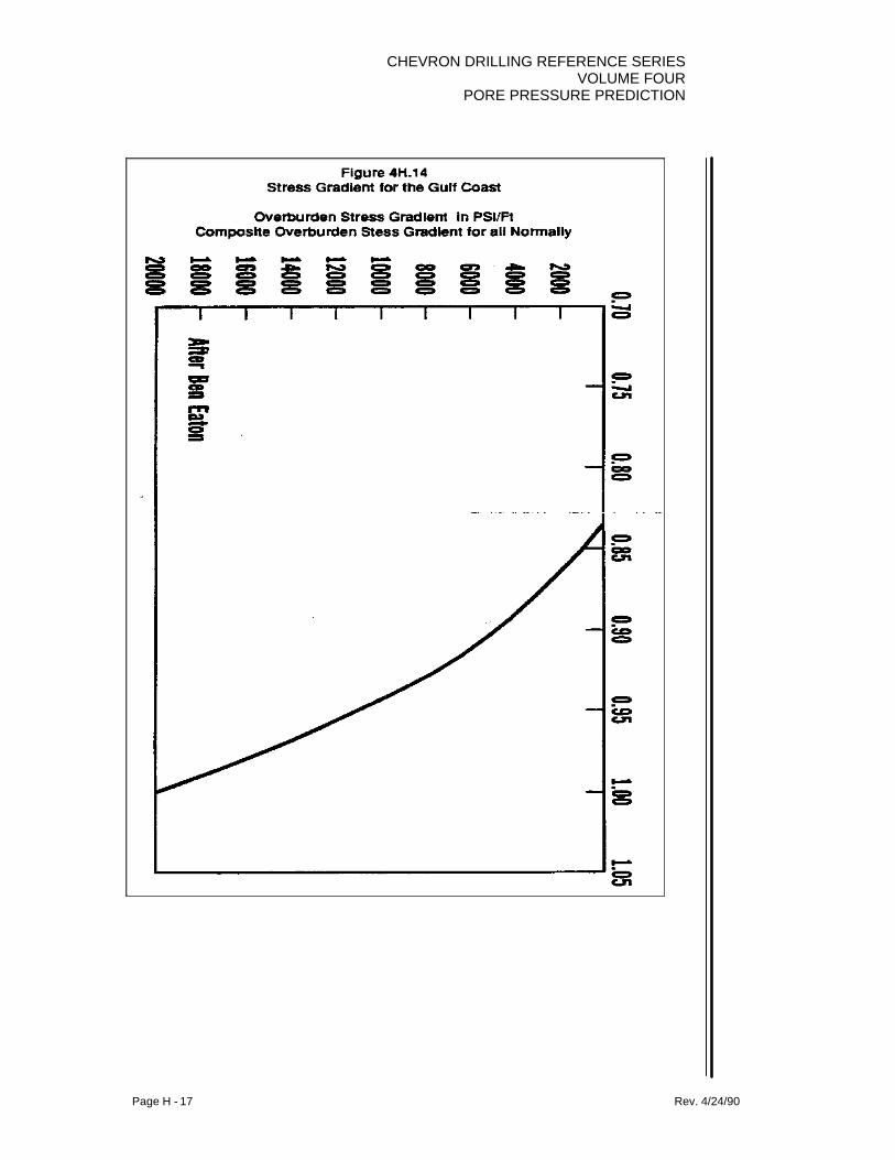
CHEVRON DRILLING REFERENCE SERIESVOLUME FOUR
PORE PRESSURE PREDICTION
Page H - 17 Rev. 4/24/90

CHEVRON DRILLING REFERENCE SERIESVOLUME FOURPORE PRESSURE PREDICTION
Page H - 18 Rev. 4/24/90
F
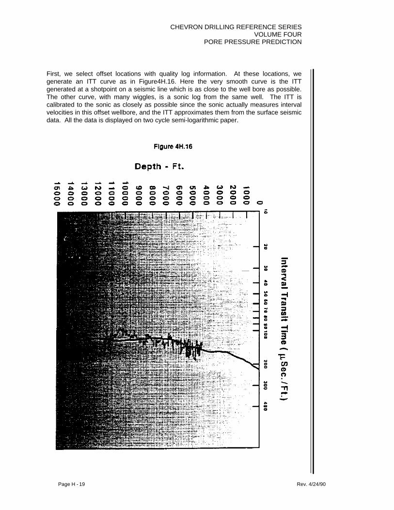
CHEVRON DRILLING REFERENCE SERIESVOLUME FOUR
PORE PRESSURE PREDICTION
Page H - 19 Rev. 4/24/90
First, we select offset locations with quality log information. At these locations, wegenerate an ITT curve as in Figure4H.16. Here the very smooth curve is the ITTgenerated at a shotpoint on a seismic line which is as close to the well bore as possible.The other curve, with many wiggles, is a sonic log from the same well. The ITT iscalibrated to the sonic as closely as possible since the sonic actually measures intervalvelocities in this offset wellbore, and the ITT approximates them from the surface seismicdata. All the data is displayed on two cycle semi-logarithmic paper.

CHEVRON DRILLING REFERENCE SERIESVOLUME FOURPORE PRESSURE PREDICTION
Page H - 20 Rev. 4/24/90
The vertical depth scale is at one inch equals one thousand feet and the horizontal logscale is in microseconds per foot. Next we generate pore pressure plots on the logs fromthis off set and determine actual pore pressures for as many intervals as possible. Wedisplay this pore pressure data next to the ITT curve as in Figure 4H.17.

CHEVRON DRILLING REFERENCE SERIESVOLUME FOUR
PORE PRESSURE PREDICTION
Page H - 21 Rev. 4/24/90
Next, we will construct a straight normal trend line through the ITT curve and calculatepore pressures using Eaton's equation. We will realign this normal trend line to whateverposition is necessary until the pore pressures derived from the ITT match those derivedfrom the logs. This is done through trial and error and may take several attempts. InFigure4H.18 we have our first attempt at drawing the normal velocity trend. We find withthis normal trend, that the pore pressures we calculate from the ITT are too high.
CHEVRON DRILLING REFERENCE SERIESVOLUME FOURPORE PRESSURE PREDICTION
Page H - 22 Rev. 4/24/90
We know from Eaton's equations, that as we bring the observed and normal values of aparameter closer together, that calculated values of pore pressures will get lower. Withthis in mind, we draw a second normal trend line parallel to the first but shifted to the rightas in Figure 4H.19. Now we find that the top of abnormal pressure coincides, ITTdetermined pore pressures at bottom are accurate, however, ITT pore pressures throughthe mid-section of the well are still too high.

CHEVRON DRILLING REFERENCE SERIESVOLUME FOUR
PORE PRESSURE PREDICTION
Page H - 23 Rev. 4/24/90
If we rotate this normal trend line of Figure 4H.19 about the point of the top of abnormalpressure as in Figure 4H.20, we find ITT indicated pore pressures are more accuratethrough the midsection of the well but are too low toward the bottom. Keep in mind that

CHEVRON DRILLING REFERENCE SERIESVOLUME FOURPORE PRESSURE PREDICTION
Page H - 24 Rev. 4/24/90
the interval velocity data determined from stacking velocity information is not precise andconsequently the ITT may be off depth and may require a depth adjustment.

CHEVRON DRILLING REFERENCE SERIESVOLUME FOUR
PORE PRESSURE PREDICTION
Page H - 25 Rev. 4/24/90
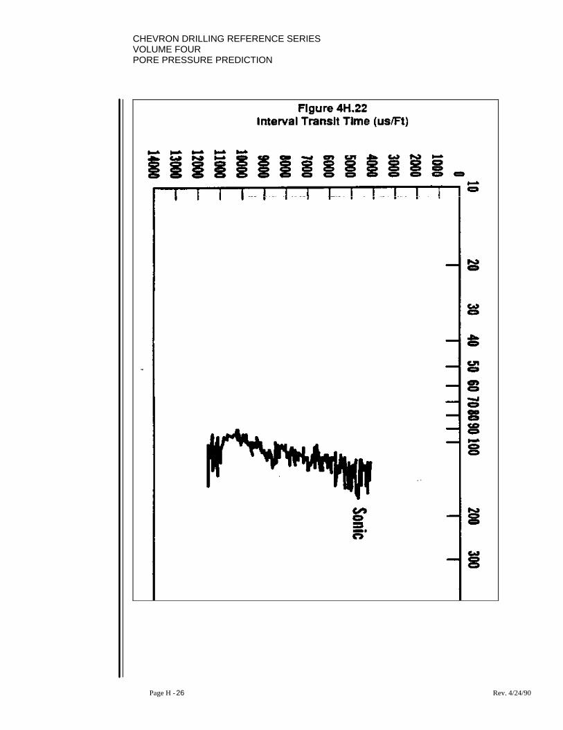
CHEVRON DRILLING REFERENCE SERIESVOLUME FOURPORE PRESSURE PREDICTION
Page H - 26 Rev. 4/24/90
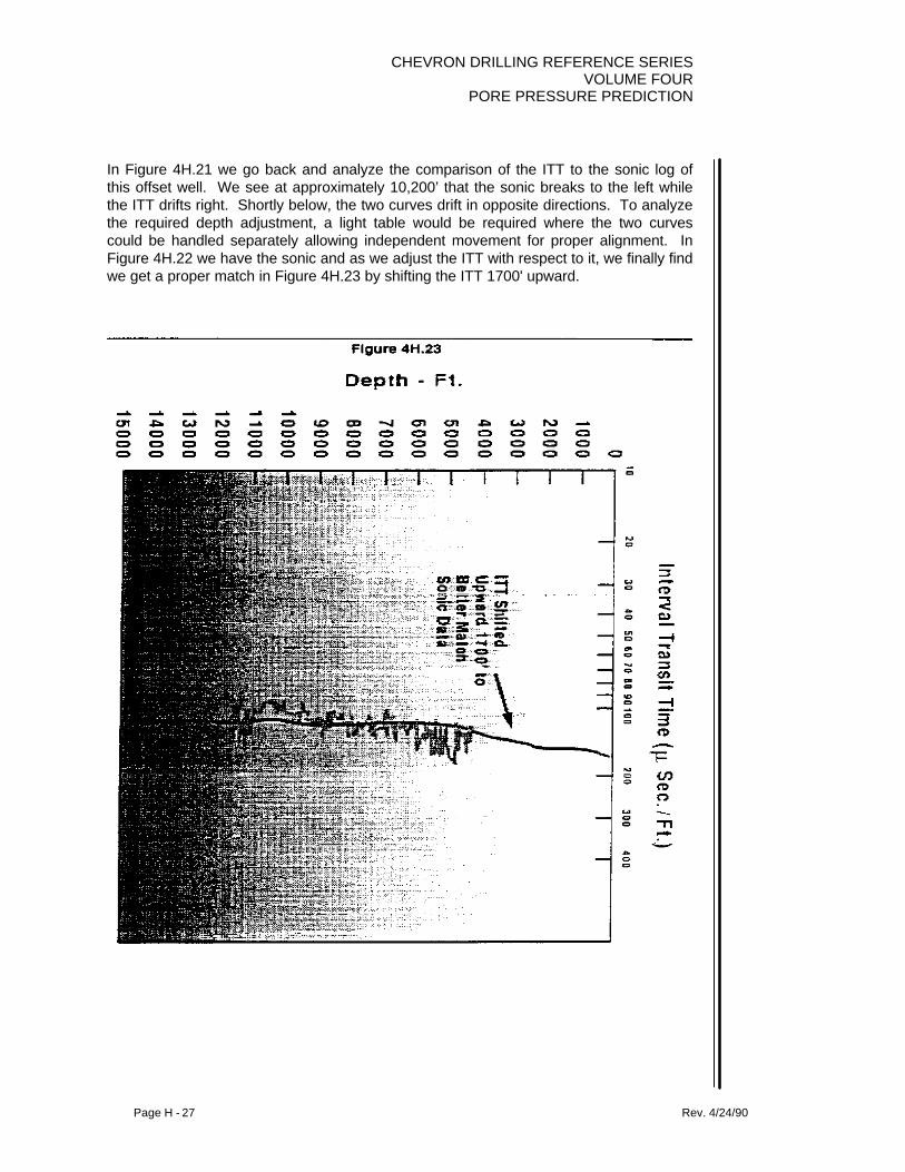
CHEVRON DRILLING REFERENCE SERIESVOLUME FOUR
PORE PRESSURE PREDICTION
Page H - 27 Rev. 4/24/90
In Figure 4H.21 we go back and analyze the comparison of the ITT to the sonic log ofthis offset well. We see at approximately 10,200’ that the sonic breaks to the left whilethe ITT drifts right. Shortly below, the two curves drift in opposite directions. To analyzethe required depth adjustment, a light table would be required where the two curvescould be handled separately allowing independent movement for proper alignment. InFigure 4H.22 we have the sonic and as we adjust the ITT with respect to it, we finally findwe get a proper match in Figure 4H.23 by shifting the ITT 1700' upward.

CHEVRON DRILLING REFERENCE SERIESVOLUME FOURPORE PRESSURE PREDICTION
Page H - 28 Rev. 4/24/90
Now the two curves break to the same directions at the same depths. We do notnormally find we require this much adjustment in most cases, but this dramatic examplepoints out the need for care. Now that we know the depth adjustment requirements weproceed with another attempt at drawing the normal velocity trend as in Figure 4H.24,realizing that pore pressure values calculated from the ITT require a 1700' adjustment.

CHEVRON DRILLING REFERENCE SERIESVOLUME FOUR
PORE PRESSURE PREDICTION
Page H - 29 Rev. 4/24/90
We find that two more attempts are required as in Figures 4H.25 and 4H.26 before wefinally arrive at a good match. We now find that pore pressures calculated from the ITTvery closely match log derived pore pressures. We now have a calibration on the normalvelocity trend through this stratigraphic interval for this particular drilling area. To be surethis is the case, we will graphically compare the results.

CHEVRON DRILLING REFERENCE SERIESVOLUME FOURPORE PRESSURE PREDICTION
Page H - 30 Rev. 4/24/90
In Figure 4H.27 we have a plot of pore pressures vs. depth from both the log properties,and from the ITT with no depth adjustment to the ITT values. As we depth adjust the ITTvalues, we arrive at Figure 4H.28. Graphically, we see a close match and feelcomfortable with the calibration of the normal velocity trend.

CHEVRON DRILLING REFERENCE SERIESVOLUME FOUR
PORE PRESSURE PREDICTION
Page H - 31 Rev. 4/24/90

CHEVRON DRILLING REFERENCE SERIESVOLUME FOURPORE PRESSURE PREDICTION
Page H - 32 Rev. 4/24/90

CHEVRON DRILLING REFERENCE SERIESVOLUME FOUR
PORE PRESSURE PREDICTION
Page H - 33 Rev. 4/24/90

CHEVRON DRILLING REFERENCE SERIESVOLUME FOURPORE PRESSURE PREDICTION
Page H - 34 Rev. 4/24/90
An alternate approach to the calibration of the normal velocity trend line can be moresimply performed by backing into, so to speak, the Eaton pressure equation. In Figure4H.29, we have an ITT curve for an off set well for which we know pore pressures fromour log analysis. These known pore pressures are listed on the left in the Figure atdepth.

CHEVRON DRILLING REFERENCE SERIESVOLUME FOUR
PORE PRESSURE PREDICTION
Page H - 35 Rev. 4/24/90
Since we know the pore pressures, the value of the pressure exponent, and theobserved values of interval travel time ( the ITT values ), we can rearrange the equationand solve for normal values of interval transit time. These would be the values of intervaltransit time for normally pressured, normally compacted rock of the same type at thesame depth. Once solving for the normal values, we can then curve fit the data pointswith the best straight line fit as in Figure 4H.30.

CHEVRON DRILLING REFERENCE SERIESVOLUME FOURPORE PRESSURE PREDICTION
Page H - 36 Rev. 4/24/90
Now we generate an ITT curve at the proposed location as in Figure 4H.30. We use thesame normal velocity trend as calibrated in the offset for the stratigraphic interval ofinterest. We use the Eaton equation for interval transit time again to compare values ofobserved to normal interval transit times and calculate pore pressures as in Figure4H.31. We realize these values require a depth adjustment as did the off set and plotthem as such in Figure 4H.32.
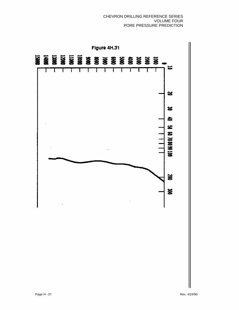
CHEVRON DRILLING REFERENCE SERIESVOLUME FOUR
PORE PRESSURE PREDICTION
Page H - 37 Rev. 4/24/90

CHEVRON DRILLING REFERENCE SERIESVOLUME FOURPORE PRESSURE PREDICTION
Page H - 38 Rev. 4/24/90

CHEVRON DRILLING REFERENCE SERIESVOLUME FOUR
PORE PRESSURE PREDICTION
Page H - 39 Rev. 4/24/90
To illustrate the value of such prediction techniques, we have included some results. InFigures 4H.34 through 4H.39, we graphically compare predictions of pore pressureutilizing this ITT technology, to both actual mud weight requirements, and actual logderived pore pressures as the wells were drilled. In each case you can see that

CHEVRON DRILLING REFERENCE SERIESVOLUME FOURPORE PRESSURE PREDICTION
Page H - 40 Rev. 4/24/90
predicted pore pressures very closely matched well requirements, and these are only afew examples of the excellent results we've seen.
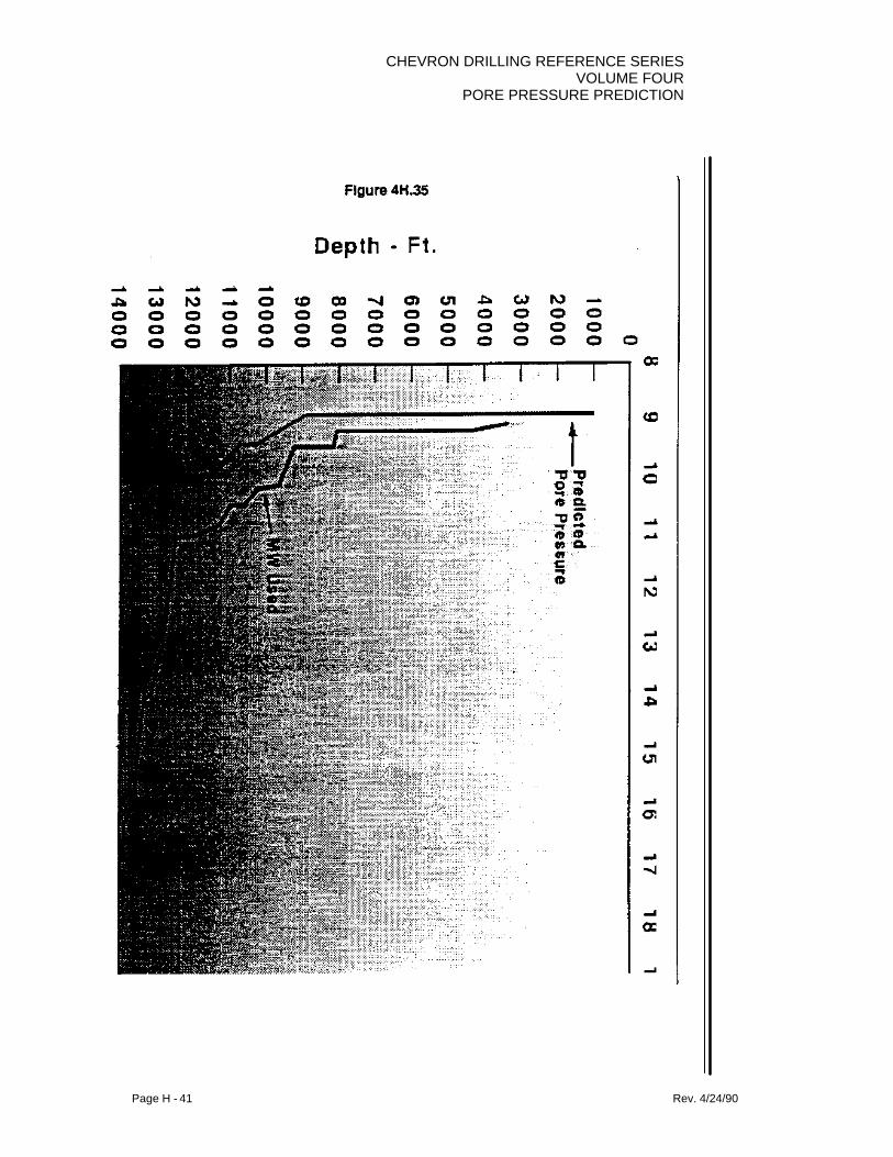
CHEVRON DRILLING REFERENCE SERIESVOLUME FOUR
PORE PRESSURE PREDICTION
Page H - 41 Rev. 4/24/90
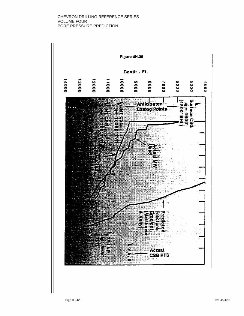
CHEVRON DRILLING REFERENCE SERIESVOLUME FOURPORE PRESSURE PREDICTION
Page H - 42 Rev. 4/24/90
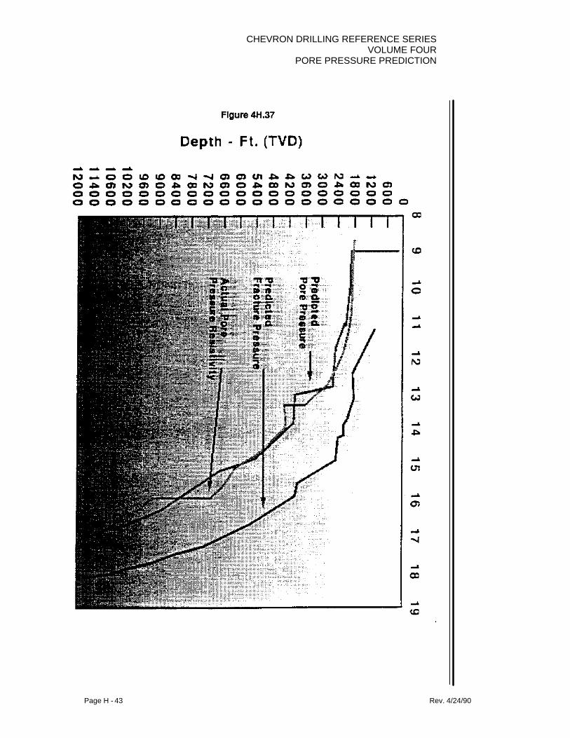
CHEVRON DRILLING REFERENCE SERIESVOLUME FOUR
PORE PRESSURE PREDICTION
Page H - 43 Rev. 4/24/90
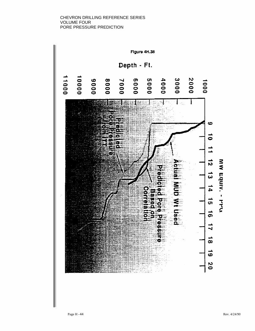
CHEVRON DRILLING REFERENCE SERIESVOLUME FOURPORE PRESSURE PREDICTION
Page H - 44 Rev. 4/24/90
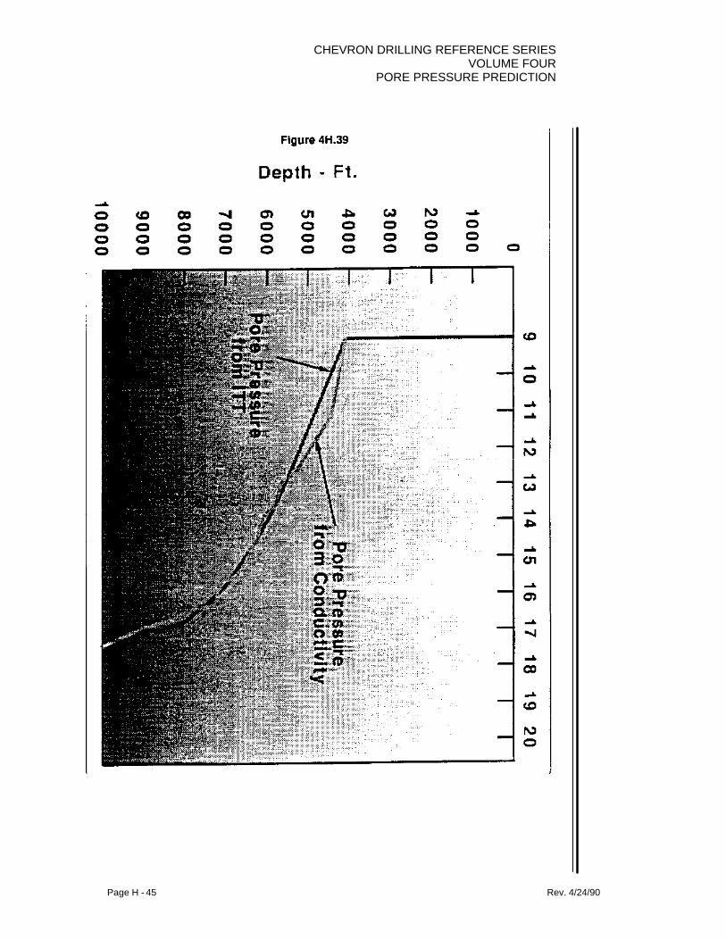
CHEVRON DRILLING REFERENCE SERIESVOLUME FOUR
PORE PRESSURE PREDICTION
Page H - 45 Rev. 4/24/90

CHEVRON DRILLING REFERENCE SERIESVOLUME FOURPORE PRESSURE PREDICTION
Page H - 46 Rev. 4/24/90
4. NOMENCLATURE
t's = Interval transit times
ITT = Interval Transit Time - A display of interval velocity vs. depth asdetermined from surface seismic data
GP = Pore pressure gradient psi/ft.
Go = Overburden gradient psi/ft.
Gn = Normal gradient psi/ft.
Ro1Co1dco1to = observed reading
Rn1Cn1dcn1 tn = normal trend reading
Gf = Fracture gradient
Ki = Matrix stress coefficient
v = Poisson's ratio
5. REFERENCES
1. E. S. Pennebaker, An Interpretation of Seismic Data, SPE paper 2165.
2. B. A. Eaton, The Equation for Geopressure Prediction from Well Logs, SPE
paper 5544.
CHEVRON DRILLING REFERENCE SERIESVOLUME FOUR
PORE PRESSURE PREDICTION
Page H - 47 Rev. 4/24/90
Pore Pressure Prediction using ITT Curves
Information Required:
1. Sonic logs displayed at 1” = 1000 ft for all offset wells to be examined, 2. ITT curves for the offset wells and the proposed location. Note, If the offset and/or
proposed wells are highly deviated, more than one ITT curve may be required atthese locations.
3. Sonic logs ( 1” = 100 ft) interpreted for pore pressure at the offset locations. Procedure:
1. For the offset wells, invert the ITT curve and place It onto the 1” = 1000’ sonic log.Correlate the ITT curve with the sonic log and transfer the re-calibration points fromthe sonic log onto the ITT. For the proposed location, correlate the re-calibrationpoints form the nearest offset, if possible. If correlation is not possible then pick re-calibration points based on abrupt changes in the ITT curve.
2. Draw the trend lines for the “shale" responses between the re-calibration points.
Note: You will need to examine the interpreted sonic log (1” = 100’) to determinewhich side of the ITT curve should be plotted. Since the ITT is typically displayedopposite of the sonic, if the sonic trend line was drawn on the left for a particularinterval. then the trend lines for that interval will be drawn on the right on the ITT.The ITT curve will not have a gamma ray displayed. On offset wells you can lay theITT next to the 1" = 100' sonic log and read the shale zones from the gamma ray,This will require correcting the ITT curve for depth, respective to the sonic log. Forthe proposed location, you will need to assume that the ITT curve response is theshale response. Note: the ITT curve for the proposed well will typically have thesame share response (i.e. left or right side of the curve) as the offset ITT curves.
3. Transfer the trend lines from the ITT curve onto two cyclo-semi-log paper. If the ITT
curve is displayed on a semi-log scale identical to your semi-log paper, you canoverlay the semi-log paper onto the ITT curve and trace the trend lines directly (alight table works great). The re-calibration points should also be transferred. Notethat it is advisable to record the ITT depth and the sonic depth determined from thecorrelation since the ITT is not depth accurate.
4. Overlay the semi-log paper with a second sheet of semi-log paper and trace the
trend lines adjusting the overlaid sheet to account for the shifting required to connect
CHEVRON DRILLING REFERENCE SERIESVOLUME FOURPORE PRESSURE PREDICTION
Page H - 48 Rev. 4/24/90
the trend lines across the re-calibration points. It is very important that the twopieces of paper maintain the same orientation during the shifting!!
5. Correct the ITT plot for depth by making an adjust identical to that required forthe ITT at the offset well (i.e. if the ITT was corrected up 1000’, at the offset,correct the ITT 1000’ up at the proposed location.)
6. Determine the normal trend line for the ITT plot. The top of pressure for an offsetwell should be the same as that for the sonic plot. Remember to correct the ITTplot for depth!!
7. If an overlay is to be created, note the depth and known pressure point(s) onto theplot (remember to plot these pressure point(s) on the sonic depth, not the ITTdepth). Determine the exponent using Eaton's equations and then calculate theobserved values for various pore pressures and plot these values on the semi-logpaper. Draw trend lines through these values parallel to the normal trend linedetermined in #5.
8. Read the pore pressure values at the inflection points from the overlay and plotthem on a pressure vs. depth plot on regular coordinate paper. Compare theresults of the ITT analysis for the proposed well, that of the pore pressuresdetermined from correlating the sonic pore pressures across the seismic line. Ifthe ITT curve compares favorably to the correlation, use the correlation. Thecorrelation is used because it typically has more "characters”.
Note: It the ITT and the sonic plots have a similar profile but the depths differ slightly,adjust the sonic plot to match the ITT. The reasoning behind this is that the ITT hasalready been adjusted for depth (step #5). We assume that the correlation is in error dueto fluid densities different than the “native” fluid density that was assumed when thecorrelation was made.
If the ITT and the correlation are not similar, use the ITT. This is an indication that thereis not a hydraulic relationship between the wells. In some instances the ITT and thecorrelation are similar for a portion of the well but deviate at some point. In this instance,use the correlation for that part of the well where the predictions are similar and use theITT for the remainder of the well.

CHEVRON DRILLING REFERENCE SERIESVOLUME FOUR
PORE PRESSURE PREDICTION
Page H - 49 Rev. 4/24/90

CHEVRON DRILLING REFERENCE SERIESVOLUME FOUR
PORE PRESSURE PREDICTION
Page I - 1 Part 1 Rev. 4/24/90
SECTION I: PREDICTING FORMATION POREPRESSURES FROM A GEOLOGICALMODELING APPROACH
1. INTRODUCTION
Drilling performance, drilling problems encountered, the success in reaching objectives,can all be directly related to the accuracy of predicted formation pore pressures. This isparticularly true when dealing with exploratory wells. Drilling the same stratigraphies asseen in offset wells does not necessarily equate to drilling the same pore pressures atdepth nor to utilizing the same casing program as these offsets. When exploratory wellsare involved, this is more likely to be true than not. Accurately predicting formation porepressures, for many wells, can be the determining factor in the mechanical success ofthe well.
This approach to prediction of formation pore pressures incorporates into it the geologicalmodel. Offset log information, structural relationships between wells from surface to totaldepth, and velocity data from surface seismic, are utilized to model the anticipated porepressures to be seen in the wellbore from surface to total depth. This modeling approachyields a reliable pore pressure scenario from which to plan a drilling program and executeoperations.
Numerous wells throughout the Gulf of Mexico as well as a number around the worldhave been analyzed with this approach with great success. The modeling approach willbe illustrated in this writing as well as results of the use of this methodology.
2. BACKGROUND
When dealing with abnormally pressured environments there are some definite structuralimpacts on the pressures to be seen in a proposed well with respect to the offsets,assuming there is a hydraulic relationship between the wells.
Dipping beds normally have no impact on pore pressure in normally pressuredenvironments. Hydrocarbons increase pore pressure as we move up dip. Bottom holepressure is lower but the pore pressure is higher in mud weight equivalent up dip. Whenin abnormally pressured environments, moving up dip results in higher pore pressures inmud weight equivalents. As we move from well to well and cross a fault, there can be aresulting change in pore pressure. It the sealing mechanism forms very rapidly, we cansee higher pore pressures on the down thrown side of the fault due to the increasedamount of overburden supported above the seal. If the sealing mechanism forms veryslowly with respect to geological time, which is the more likely case, the opposite may betrue in that the up-thrown side can be the higher pore pressure. This results from the
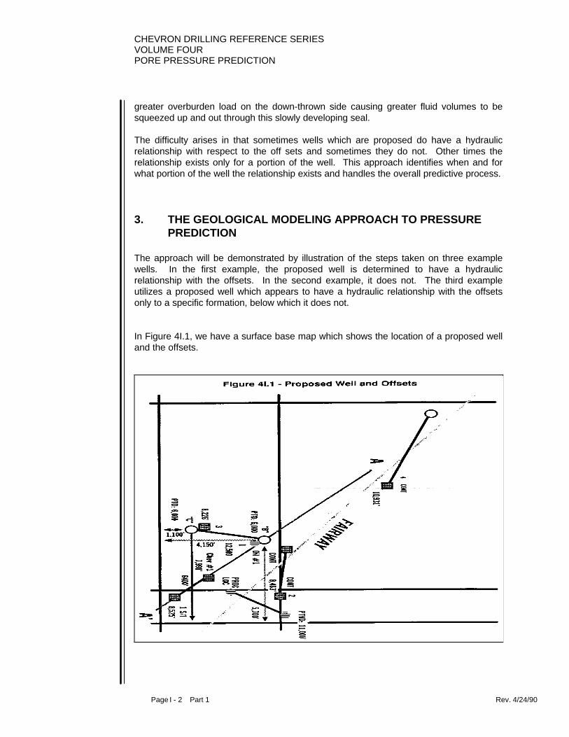
CHEVRON DRILLING REFERENCE SERIESVOLUME FOURPORE PRESSURE PREDICTION
Page I - 2 Part 1 Rev. 4/24/90
greater overburden load on the down-thrown side causing greater fluid volumes to besqueezed up and out through this slowly developing seal.
The difficulty arises in that sometimes wells which are proposed do have a hydraulicrelationship with respect to the off sets and sometimes they do not. Other times therelationship exists only for a portion of the well. This approach identifies when and forwhat portion of the well the relationship exists and handles the overall predictive process.
3. THE GEOLOGICAL MODELING APPROACH TO PRESSUREPREDICTION
The approach will be demonstrated by illustration of the steps taken on three examplewells. In the first example, the proposed well is determined to have a hydraulicrelationship with the offsets. In the second example, it does not. The third exampleutilizes a proposed well which appears to have a hydraulic relationship with the offsetsonly to a specific formation, below which it does not.
In Figure 4I.1, we have a surface base map which shows the location of a proposed welland the offsets.
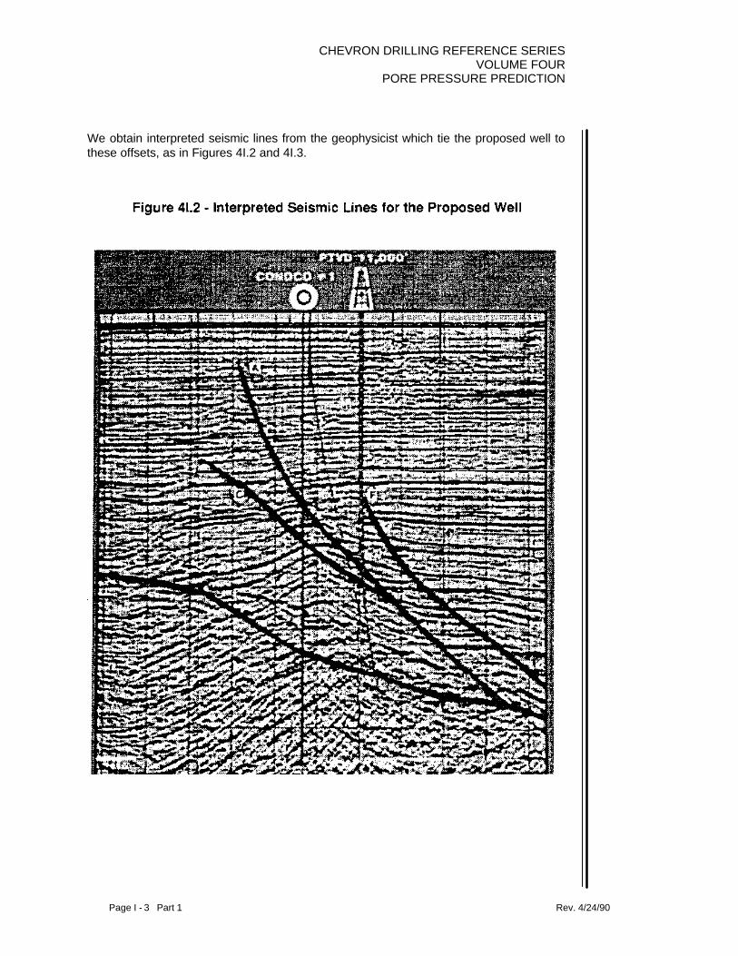
CHEVRON DRILLING REFERENCE SERIESVOLUME FOUR
PORE PRESSURE PREDICTION
Page I - 3 Part 1 Rev. 4/24/90
We obtain interpreted seismic lines from the geophysicist which tie the proposed well tothese offsets, as in Figures 4I.2 and 4I.3.
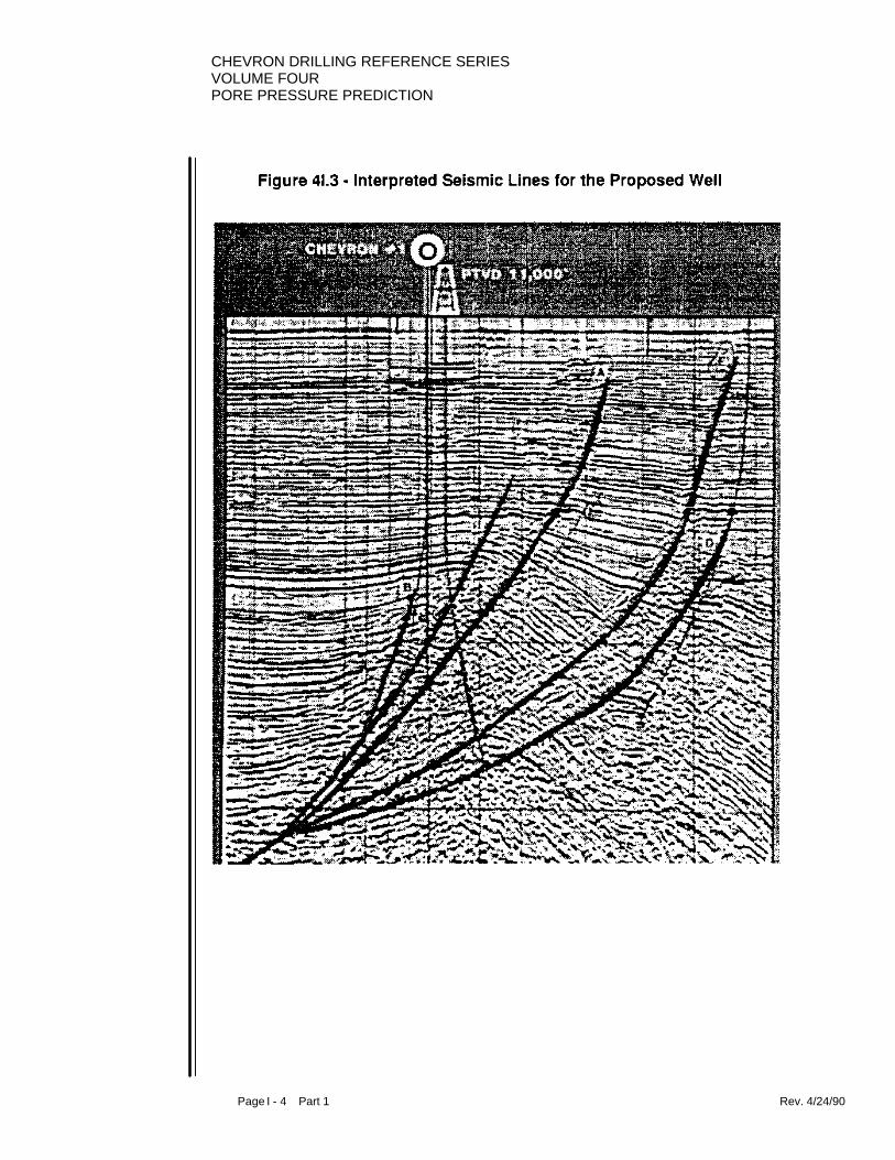
CHEVRON DRILLING REFERENCE SERIESVOLUME FOURPORE PRESSURE PREDICTION
Page I - 4 Part 1 Rev. 4/24/90
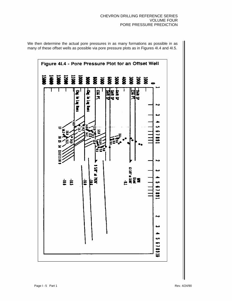
CHEVRON DRILLING REFERENCE SERIESVOLUME FOUR
PORE PRESSURE PREDICTION
Page I - 5 Part 1 Rev. 4/24/90
We then determine the actual pore pressures in as many formations as possible in asmany of these offset wells as possible via pore pressure plots as in Figures 4I.4 and 4I.5.

CHEVRON DRILLING REFERENCE SERIESVOLUME FOURPORE PRESSURE PREDICTION
Page I - 6 Part 1 Rev. 4/24/90
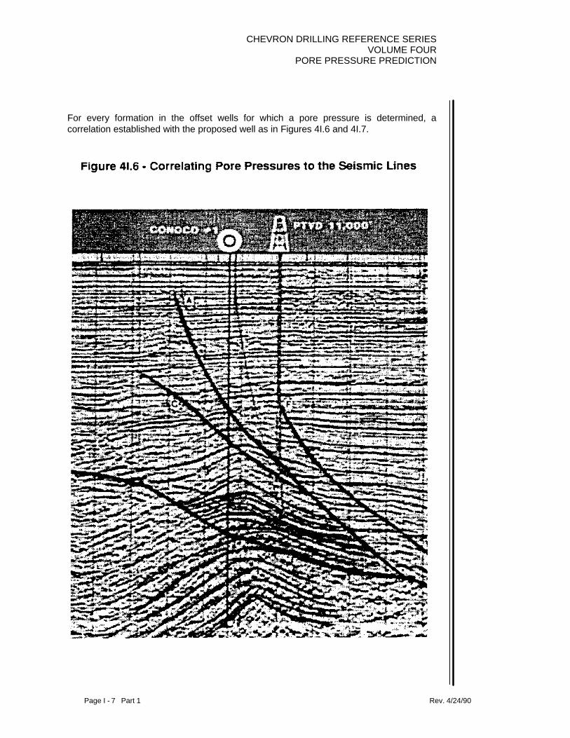
CHEVRON DRILLING REFERENCE SERIESVOLUME FOUR
PORE PRESSURE PREDICTION
Page I - 7 Part 1 Rev. 4/24/90
For every formation in the offset wells for which a pore pressure is determined, acorrelation established with the proposed well as in Figures 4I.6 and 4I.7.
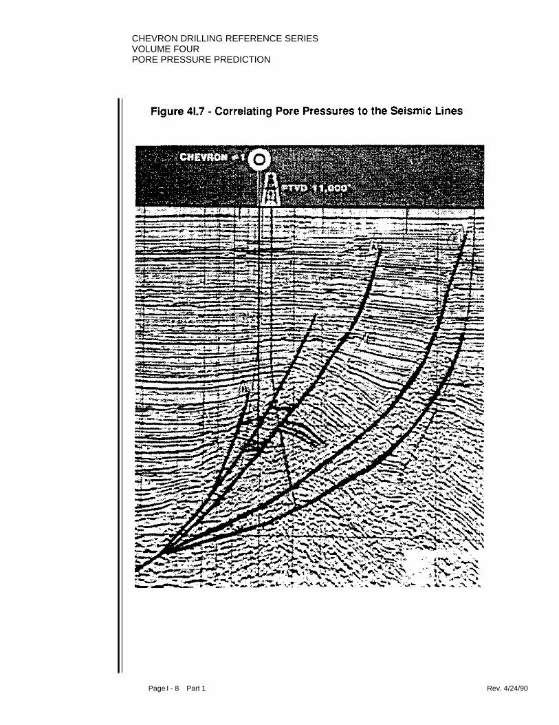
CHEVRON DRILLING REFERENCE SERIESVOLUME FOURPORE PRESSURE PREDICTION
Page I - 8 Part 1 Rev. 4/24/90

CHEVRON DRILLING REFERENCE SERIESVOLUME FOUR
PORE PRESSURE PREDICTION
Page I - 9 Part 1 Rev. 4/24/90
At this point, we assume there is a hydraulic relationship between wells. Using the nativefluid gradient for the area, we calculate anticipated pore pressures at the proposedlocation for all formations correlated. This is done by taking the difference in the depthbelow datum the formations are seen in each well and correcting bottom hole pressurefor that formation by the gradient of the native fluid for the area. This has been done inFigures 4I.8 and 4I.9.
Figure 4I.8
Calculating Anticipated Pore Pressures
Offset Well Proposed Well
Depth PP Time TimeTVD
Depth PP
7100 9.0 2.014 2.16 7700 9.07550 9.5 2.12 2.26 8100 9.57700 11.0 2.158 2.29 8225 10.97825 12.0 2.19 2.35 8450 11.87975 12.0 2.23 2.37 8525 11.98150 12.8 2.274 2.39 8600 12.68400 13.5 2.336 2.41 8700 13.48700 13.8 2.412 2.44 8800 13.88950 14.2 2.476 2.48 8975 14.29150 14.3 2.528 2.54 9200 14.39525 14.3 2.624 2.63 9550 14.310075 14.7 2.766 2.81 10250 14.610625 14.9 2.898 2.92 10725 14.911100 14.9 2.99 2.97 11000 15.011750 15.6 3.114 3.06 11465 15.812050 16.0 3.17 3.11 11725 16.212225 16.3 3.202 3.19 12150 16.4
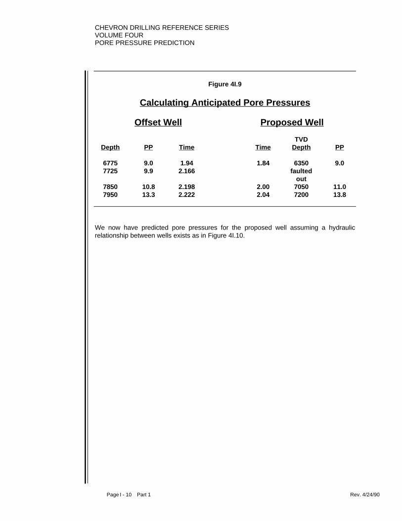
CHEVRON DRILLING REFERENCE SERIESVOLUME FOURPORE PRESSURE PREDICTION
Page I - 10 Part 1 Rev. 4/24/90
Figure 4I.9
Calculating Anticipated Pore Pressures
Offset Well Proposed Well
Depth PP Time TimeTVD
Depth PP
6775 9.0 1.94 1.84 6350 9.07725 9.9 2.166 faulted
out7850 10.8 2.198 2.00 7050 11.07950 13.3 2.222 2.04 7200 13.8
We now have predicted pore pressures for the proposed well assuming a hydraulicrelationship between wells exists as in Figure 4I.10.

CHEVRON DRILLING REFERENCE SERIESVOLUME FOUR
PORE PRESSURE PREDICTION
Page I - 11 Part 1 Rev. 4/24/90
We then generate ITT ( interval transit time ) curves at the offset wells as well as at theproposed location. These ITT curves are generated from the surface seismic data. Theyare essentially synthetic sonic logs which approximate interval velocities with respect todepth. The ITT curves generated at the offset wells are calibrated to the sonic logs asclosely as possible as in Figure 4I. 11.

CHEVRON DRILLING REFERENCE SERIESVOLUME FOURPORE PRESSURE PREDICTION
Page I - 12 Part 1 Rev. 4/24/90
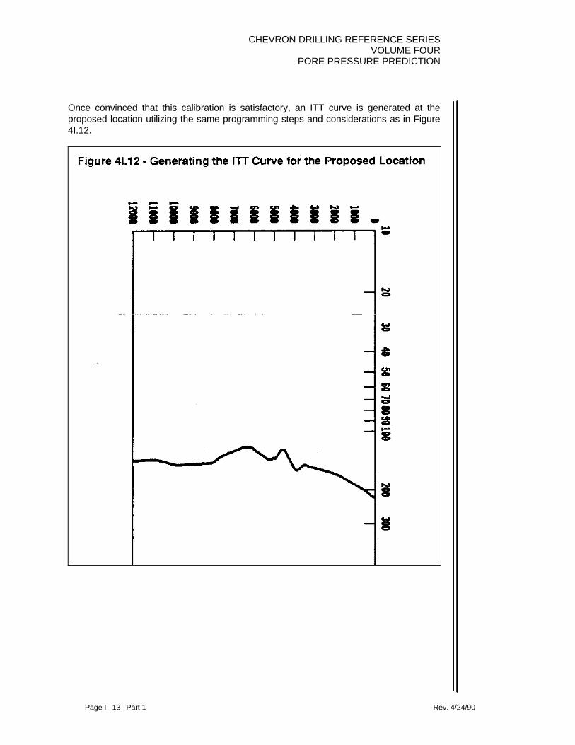
CHEVRON DRILLING REFERENCE SERIESVOLUME FOUR
PORE PRESSURE PREDICTION
Page I - 13 Part 1 Rev. 4/24/90
Once convinced that this calibration is satisfactory, an ITT curve is generated at theproposed location utilizing the same programming steps and considerations as in Figure4I.12.

CHEVRON DRILLING REFERENCE SERIESVOLUME FOURPORE PRESSURE PREDICTION
Page I - 14 Part 1 Rev. 4/24/90
The ITT curves at the offsets are calibrated to the known pore pressures to exist in theseoffsets as in Figure 4I.13, until a match between pore pressures derived from the ITT andthose derived from log properties is obtained as closely as possible as in Figure 4I.14.

CHEVRON DRILLING REFERENCE SERIESVOLUME FOUR
PORE PRESSURE PREDICTION
Page I - 15 Part 1 Rev. 4/24/90
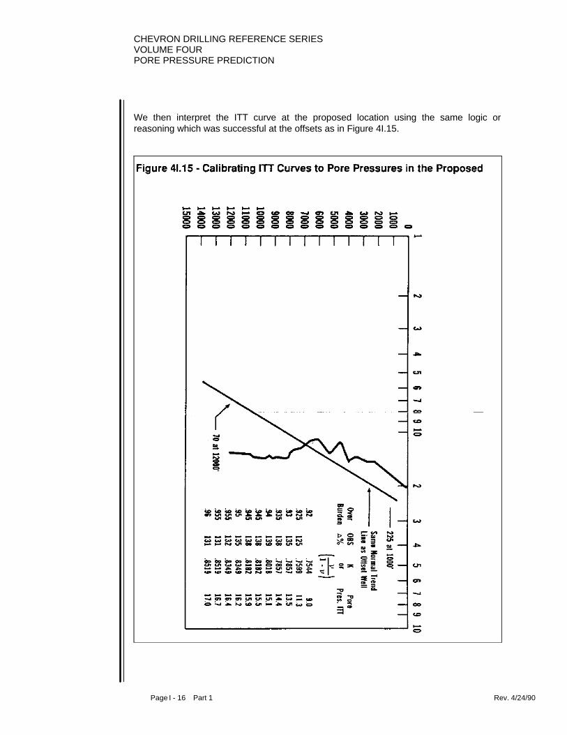
CHEVRON DRILLING REFERENCE SERIESVOLUME FOURPORE PRESSURE PREDICTION
Page I - 16 Part 1 Rev. 4/24/90
We then interpret the ITT curve at the proposed location using the same logic orreasoning which was successful at the offsets as in Figure 4I.15.

CHEVRON DRILLING REFERENCE SERIESVOLUME FOUR
PORE PRESSURE PREDICTION
Page I - 17 Part 1 Rev. 4/24/90
Next we compare pore pressures predicted from the ITT at the proposed location tothose predicted by correlation which assumed a hydraulic relationship between wells toexist as in Figure 4I.16. Here we see that the two curves match quite nicely whichverifies the hydraulic relationship.

CHEVRON DRILLING REFERENCE SERIESVOLUME FOURPORE PRESSURE PREDICTION
Page I - 18 Part 1 Rev. 4/24/90
However, the fluid gradient assumed may have been slightly different or correlations mayhave deviated slightly yielding the difference seen between the two curves.Consequently, the correlative scenario is shifted upward to coincide with the ITT scenarioas in Figure 4I.17, and this newly placed correlative scenario becomes the predicted porepressure curve for the proposed well.
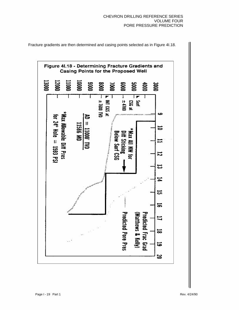
CHEVRON DRILLING REFERENCE SERIESVOLUME FOUR
PORE PRESSURE PREDICTION
Page I - 19 Part 1 Rev. 4/24/90
Fracture gradients are then determined and casing points selected as in Figure 4I.18.

CHEVRON DRILLING REFERENCE SERIESVOLUME FOURPORE PRESSURE PREDICTION
Page I - 20 Part 1 Rev. 4/24/90
The actual mud weights required to drill this well as well as actual pore pressures seenvs. predicted pore pressures appear in Figure 4I.19.

CHEVRON DRILLING REFERENCE SERIESVOLUME FOUR
PORE PRESSURE PREDICTION
Page I - 21 Part 1 Rev. 4/24/90
In Figure 4I.20 we have a structure map for an area with a proposed location justsoutheast of center.

CHEVRON DRILLING REFERENCE SERIESVOLUME FOURPORE PRESSURE PREDICTION
Page I - 22 Part 1 Rev. 4/24/90
An available offset well appears to the north east of this location. Pore pressuresdetermined for this offset well appear in Figure 4I.21.

CHEVRON DRILLING REFERENCE SERIESVOLUME FOUR
PORE PRESSURE PREDICTION
Page I - 23 Part 1 Rev. 4/24/90
We correlate all formations for which pore pressures have been determined to theproposed well through the seismic ties as in Figure 4I.22.
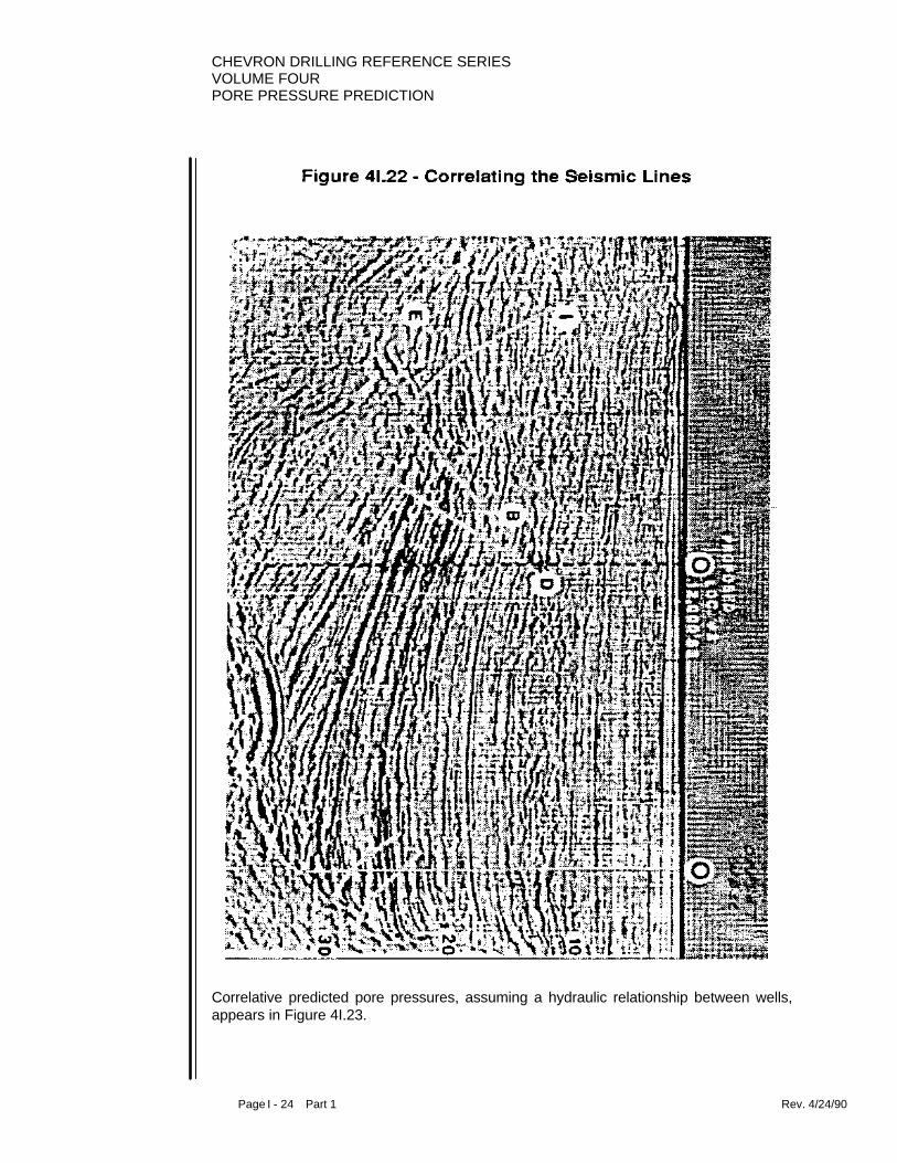
CHEVRON DRILLING REFERENCE SERIESVOLUME FOURPORE PRESSURE PREDICTION
Page I - 24 Part 1 Rev. 4/24/90
Correlative predicted pore pressures, assuming a hydraulic relationship between wells,appears in Figure 4I.23.
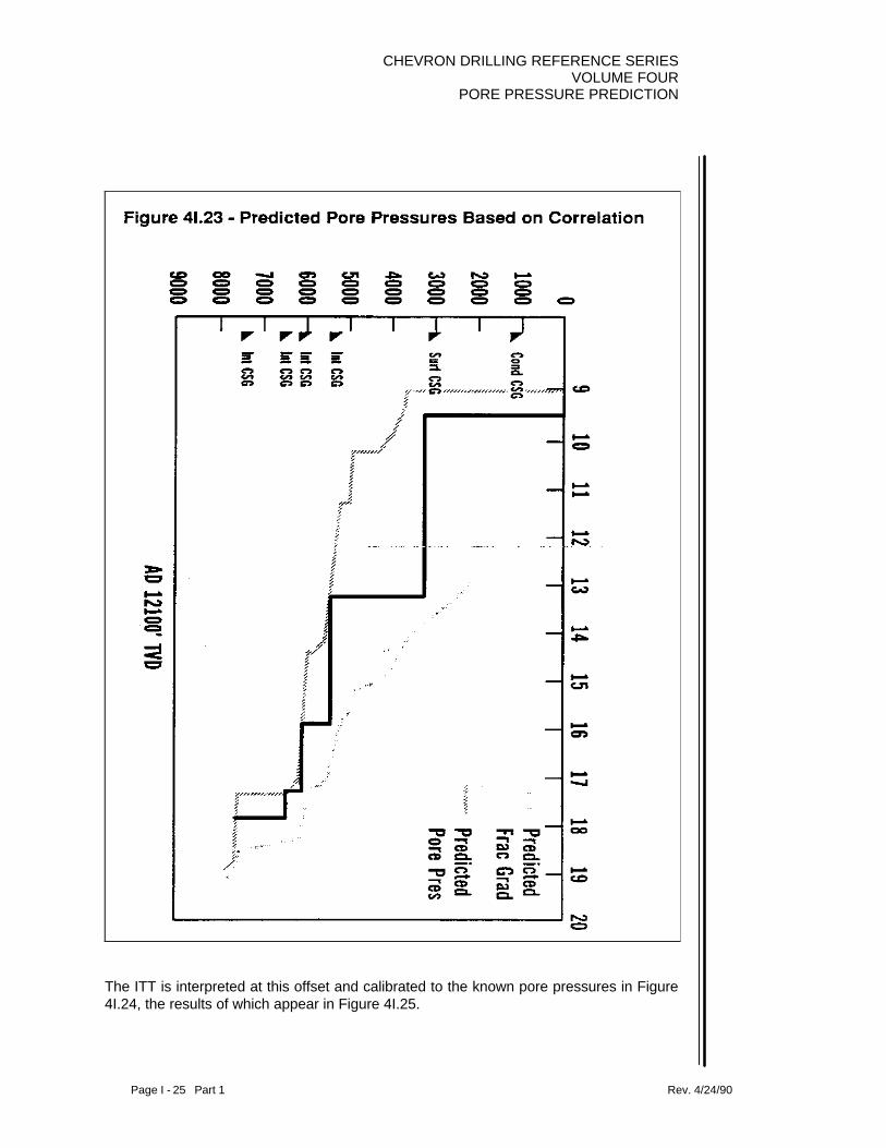
CHEVRON DRILLING REFERENCE SERIESVOLUME FOUR
PORE PRESSURE PREDICTION
Page I - 25 Part 1 Rev. 4/24/90
The ITT is interpreted at this offset and calibrated to the known pore pressures in Figure4I.24, the results of which appear in Figure 4I.25.

CHEVRON DRILLING REFERENCE SERIESVOLUME FOURPORE PRESSURE PREDICTION
Page I - 26 Part 1 Rev. 4/24/90

CHEVRON DRILLING REFERENCE SERIESVOLUME FOUR
PORE PRESSURE PREDICTION
Page I - 27 Part 1 Rev. 4/24/90
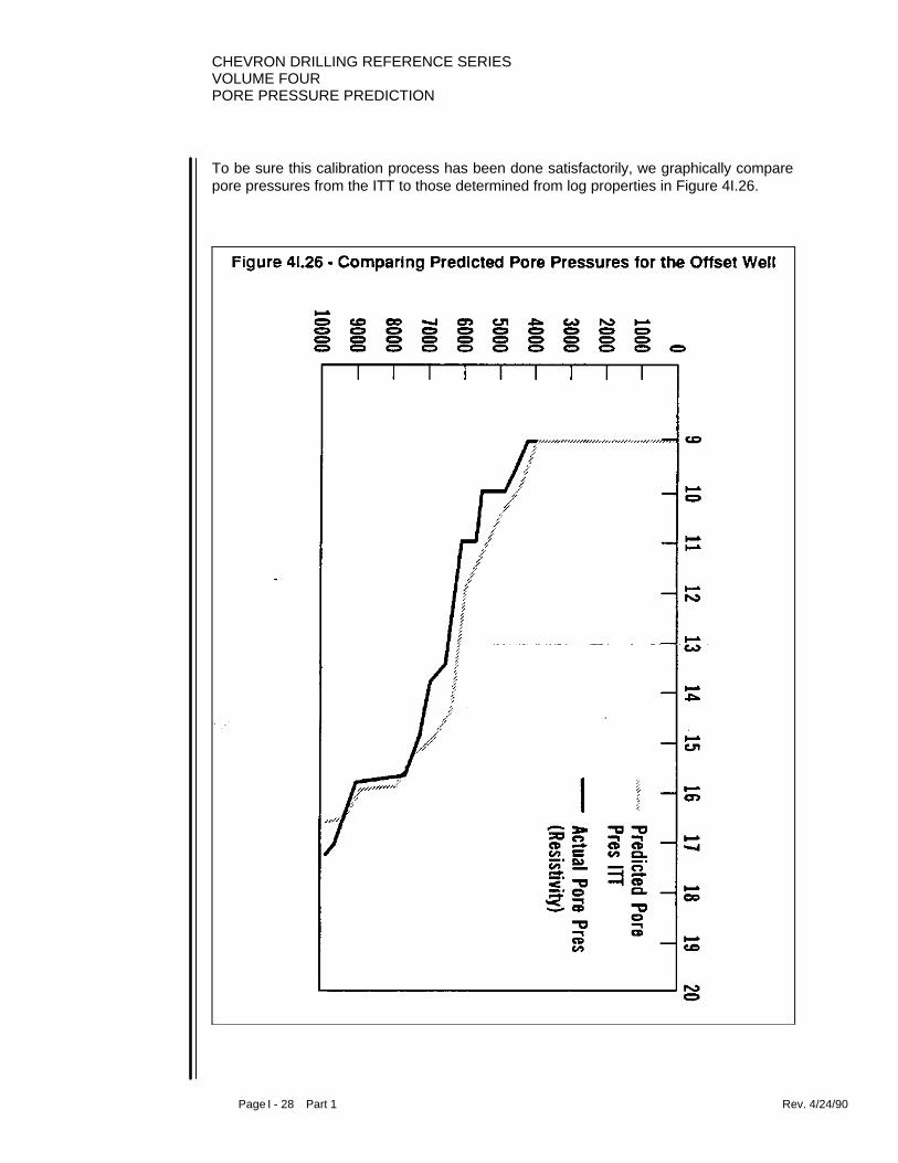
CHEVRON DRILLING REFERENCE SERIESVOLUME FOURPORE PRESSURE PREDICTION
Page I - 28 Part 1 Rev. 4/24/90
To be sure this calibration process has been done satisfactorily, we graphically comparepore pressures from the ITT to those determined from log properties in Figure 4I.26.
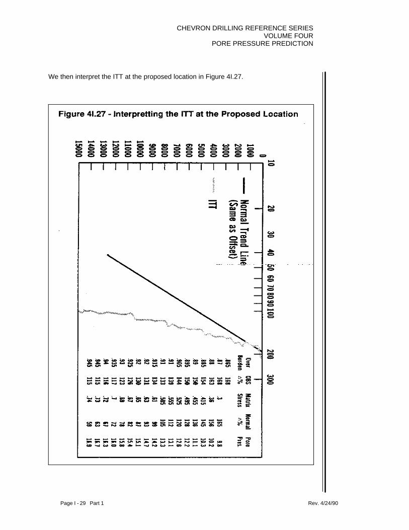
CHEVRON DRILLING REFERENCE SERIESVOLUME FOUR
PORE PRESSURE PREDICTION
Page I - 29 Part 1 Rev. 4/24/90
We then interpret the ITT at the proposed location in Figure 4I.27.
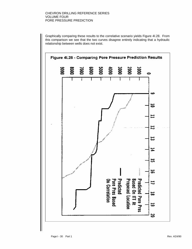
CHEVRON DRILLING REFERENCE SERIESVOLUME FOURPORE PRESSURE PREDICTION
Page I - 30 Part 1 Rev. 4/24/90
Graphically comparing these results to the correlative scenario yields Figure 4I.28. Fromthis comparison we see that the two curves disagree entirely indicating that a hydraulicrelationship between wells does not exist.

CHEVRON DRILLING REFERENCE SERIESVOLUME FOUR
PORE PRESSURE PREDICTION
Page I - 31 Part 1 Rev. 4/24/90
The ITT predicted pore pressures become the only scenario from which to plan theproposed well. This is done in Figure 4I.29.

CHEVRON DRILLING REFERENCE SERIESVOLUME FOURPORE PRESSURE PREDICTION
Page I - 32 Part 1 Rev. 4/24/90
A comparison of pore pressures predicted for this well and those actually seen based onlog properties appears in Figure 4I.30.

CHEVRON DRILLING REFERENCE SERIESVOLUME FOUR
PORE PRESSURE PREDICTION
Page I - 33 Part 1 Rev. 4/24/90
A comparison to actual mud weights required during drilling appears in Figure 4I.31.

CHEVRON DRILLING REFERENCE SERIESVOLUME FOURPORE PRESSURE PREDICTION
Page I - 34 Part 1 Rev. 4/24/90
In Figure 4I.32, we have selected lithology tops for an offset well from the gamma rayand sonic logs.

CHEVRON DRILLING REFERENCE SERIESVOLUME FOUR
PORE PRESSURE PREDICTION
Page I - 35 Part 1 Rev. 4/24/90
Sonic velocity trends within lithological sections are then determined as in Figure 4I.33.

CHEVRON DRILLING REFERENCE SERIESVOLUME FOURPORE PRESSURE PREDICTION
Page I - 36 Part 1 Rev. 4/24/90
Pore pressures for all formations are then determined for this offset as in Figure 4I.34and are compared to mud weights used in Figure 4I.35.

CHEVRON DRILLING REFERENCE SERIESVOLUME FOUR
PORE PRESSURE PREDICTION
Page I - 37 Part 1 Rev. 4/24/90

CHEVRON DRILLING REFERENCE SERIESVOLUME FOURPORE PRESSURE PREDICTION
Page I - 38 Part 1 Rev. 4/24/90
Again for as many formation as possible, correlations are established between wellsthrough seismic ties (not shown for this example). Pore pressures are calculated for theproposed well assuming a hydraulic relationship as in Figure 4I.36.
Figure 4I.36
Predicting Pore Pressures for a Proposed Well
Offset Well Proposed Location
Depth PPTwo way
TimeTwo way
Time Depth PP
7550 9.0 1.98 1.96 7204 9.09300 12.2 2.47 2.34 9039 12.309850 13.6 2.48 2.36 9137 13.9610600 13.6 2.63 2.52 9899 13.9311300 16.7 2.76 2.68 10657 17.1711600 16.7 2.82 2.76 11036 17.0911900 16.8 2.89 2.79 1178 16.6412500 17.0 3.04 3.07 12494 17.0013300 17.0 3.22 3.28 13517 16.8713700 17.6 3.30 -- -- --14600 18.0 3.48 -- -- --14800 17.7 3.53 -- -- --14900 17.8 3.55 3.32 13723 18.5615300 18.2 3.63 3.39 14084 18.9916400 18.3 3.83 3.74 16023 18.5217000 18.4 3.94 3.93 17184 18.3018200 18.518700 18.519400 18.6
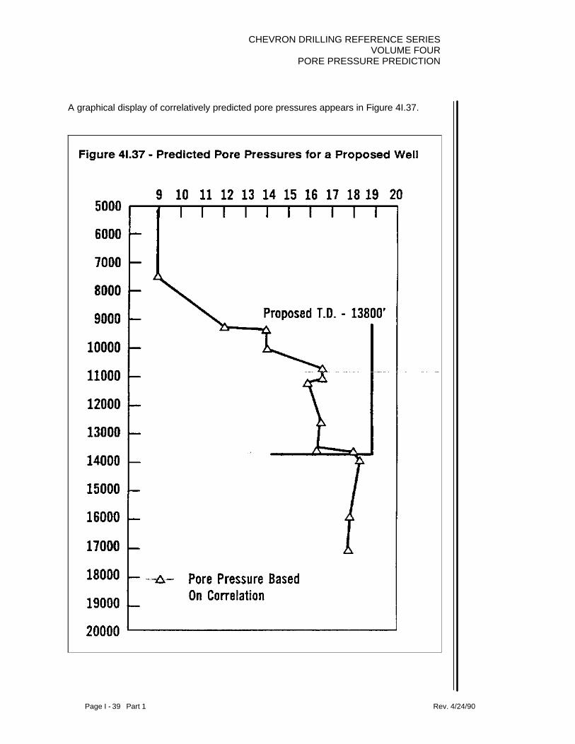
CHEVRON DRILLING REFERENCE SERIESVOLUME FOUR
PORE PRESSURE PREDICTION
Page I - 39 Part 1 Rev. 4/24/90
A graphical display of correlatively predicted pore pressures appears in Figure 4I.37.
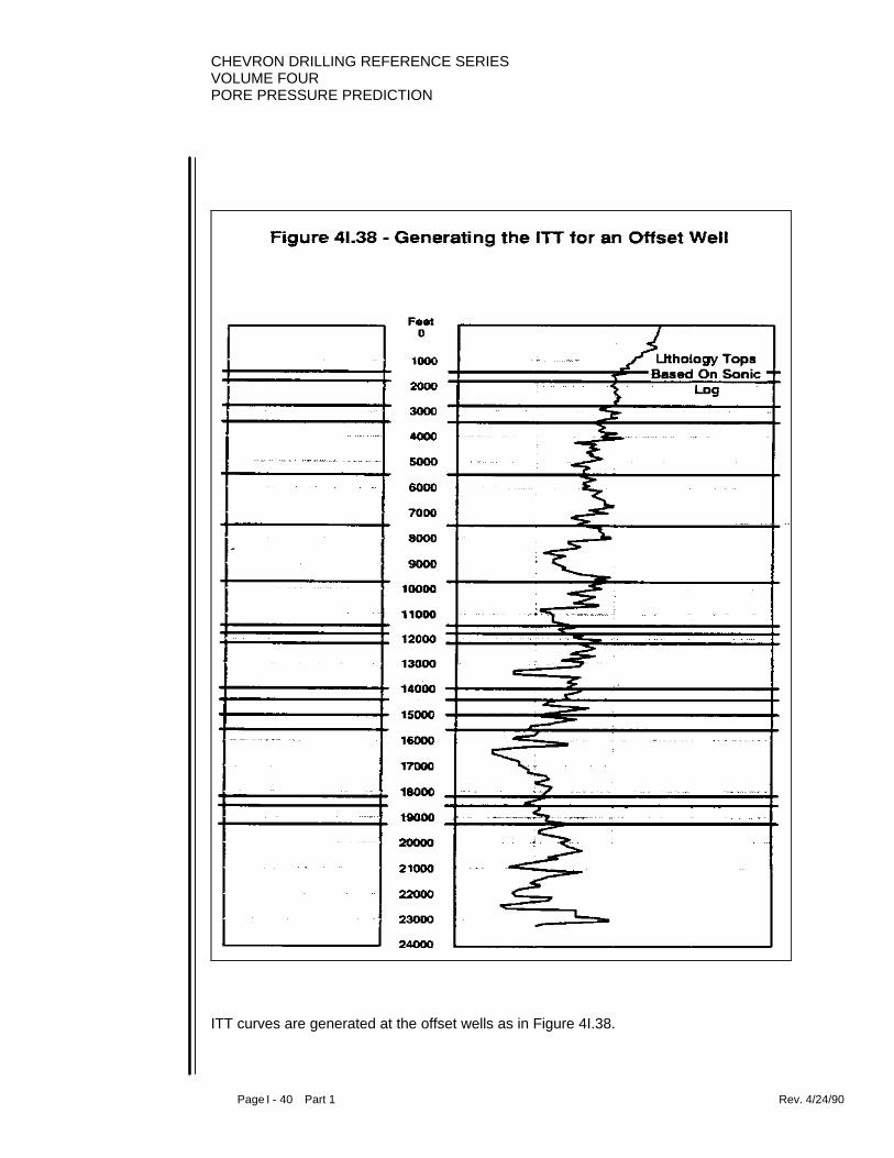
CHEVRON DRILLING REFERENCE SERIESVOLUME FOURPORE PRESSURE PREDICTION
Page I - 40 Part 1 Rev. 4/24/90
ITT curves are generated at the offset wells as in Figure 4I.38.
CHEVRON DRILLING REFERENCE SERIESVOLUME FOUR
PORE PRESSURE PREDICTION
Page I - 41 Part 1 Rev. 4/24/90
continued as 4sec_I_b.doc
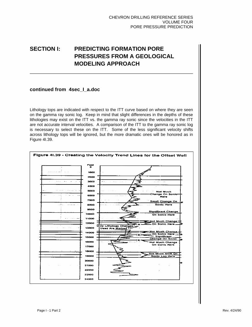
CHEVRON DRILLING REFERENCE SERIESVOLUME FOUR
PORE PRESSURE PREDICTION
Page I - 1 Part 2 Rev. 4/24/90
SECTION I: PREDICTING FORMATION POREPRESSURES FROM A GEOLOGICALMODELING APPROACH
continued from 4sec_I_a.doc
Lithology tops are indicated with respect to the ITT curve based on where they are seenon the gamma ray sonic log. Keep in mind that slight differences in the depths of theselithologies may exist on the ITT vs. the gamma ray sonic since the velocities in the ITTare not accurate interval velocities. A comparison of the ITT to the gamma ray sonic logis necessary to select these on the ITT. Some of the less significant velocity shiftsacross lithology tops will be ignored, but the more dramatic ones will be honored as inFigure 4I.39.

CHEVRON DRILLING REFERENCE SERIESVOLUME FOURPORE PRESSURE PREDICTION
Page I - 2 Part 2 Rev. 4/24/90
Recalibration of the ITT velocity trends appears in Figure 4I.40.
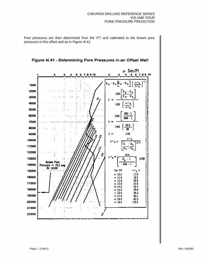
CHEVRON DRILLING REFERENCE SERIESVOLUME FOUR
PORE PRESSURE PREDICTION
Page I - 3 Part 2 Rev. 4/24/90
Pore pressures are then determined from the ITT and calibrated to the known porepressures in this offset well as in Figure 4I.41.
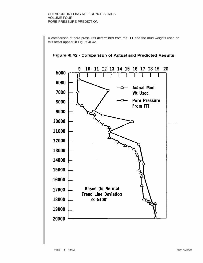
CHEVRON DRILLING REFERENCE SERIESVOLUME FOURPORE PRESSURE PREDICTION
Page I - 4 Part 2 Rev. 4/24/90
A comparison of pore pressures determined from the ITT and the mud weights used onthis offset appear in Figure 4I.42.
CHEVRON DRILLING REFERENCE SERIESVOLUME FOUR
PORE PRESSURE PREDICTION
Page I - 5 Part 2 Rev. 4/24/90
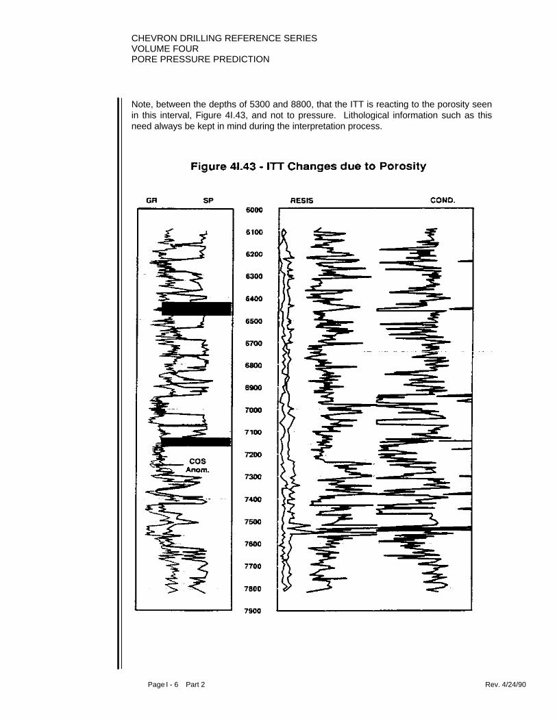
CHEVRON DRILLING REFERENCE SERIESVOLUME FOURPORE PRESSURE PREDICTION
Page I - 6 Part 2 Rev. 4/24/90
Note, between the depths of 5300 and 8800, that the ITT is reacting to the porosity seenin this interval, Figure 4I.43, and not to pressure. Lithological information such as thisneed always be kept in mind during the interpretation process.

CHEVRON DRILLING REFERENCE SERIESVOLUME FOUR
PORE PRESSURE PREDICTION
Page I - 7 Part 2 Rev. 4/24/90
An ITT is generated at the proposed location and lithological tops which dictate arecalibration in velocity trends are correlated through seismic ties and indicated as inFigure 4I.44.

CHEVRON DRILLING REFERENCE SERIESVOLUME FOURPORE PRESSURE PREDICTION
Page I - 8 Part 2 Rev. 4/24/90

CHEVRON DRILLING REFERENCE SERIESVOLUME FOUR
PORE PRESSURE PREDICTION
Page I - 9 Part 2 Rev. 4/24/90
ITT velocity trends are determined as before in Figure 4I.45 and are recalibrated into acontinuous curve as in Figure 4I.46.

CHEVRON DRILLING REFERENCE SERIESVOLUME FOURPORE PRESSURE PREDICTION
Page I - 10 Part 2 Rev. 4/24/90

CHEVRON DRILLING REFERENCE SERIESVOLUME FOUR
PORE PRESSURE PREDICTION
Page I - 11 Part 2 Rev. 4/24/90
The ITT is interpreted at the proposed location using the same reasoning which wassuccessful at the offsets as in Figure 4I.47, and the results of which appear in Figure4I.48.

CHEVRON DRILLING REFERENCE SERIESVOLUME FOURPORE PRESSURE PREDICTION
Page I - 12 Part 2 Rev. 4/24/90

CHEVRON DRILLING REFERENCE SERIESVOLUME FOUR
PORE PRESSURE PREDICTION
Page I - 13 Part 2 Rev. 4/24/90

CHEVRON DRILLING REFERENCE SERIESVOLUME FOURPORE PRESSURE PREDICTION
Page I - 14 Part 2 Rev. 4/24/90
Ignoring the interval of porosity effect yields Figure 4I.49.
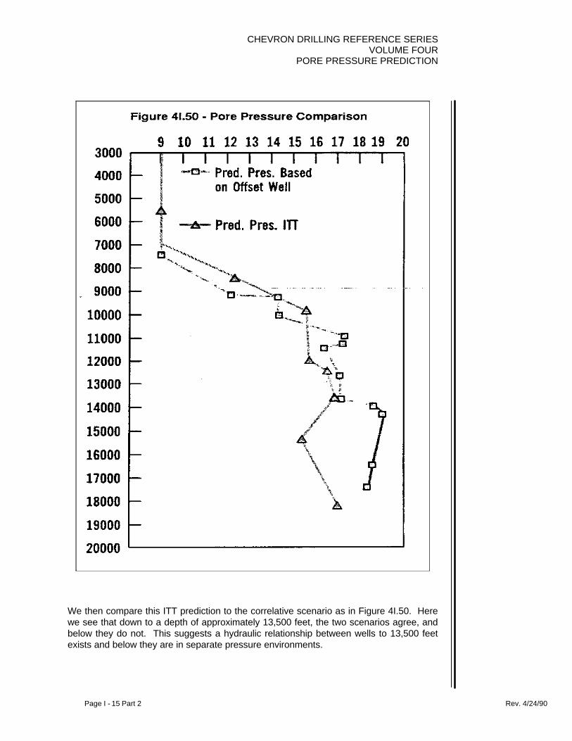
CHEVRON DRILLING REFERENCE SERIESVOLUME FOUR
PORE PRESSURE PREDICTION
Page I - 15 Part 2 Rev. 4/24/90
We then compare this ITT prediction to the correlative scenario as in Figure 4I.50. Herewe see that down to a depth of approximately 13,500 feet, the two scenarios agree, andbelow they do not. This suggests a hydraulic relationship between wells to 13,500 feetexists and below they are in separate pressure environments.

CHEVRON DRILLING REFERENCE SERIESVOLUME FOURPORE PRESSURE PREDICTION
Page I - 16 Part 2 Rev. 4/24/90
We, therefore, use the correlative information down to the depth of 13,500 feet and theITT prediction below yielding Figure 4I.51 as our predicted pore pressure profile for thewell.

CHEVRON DRILLING REFERENCE SERIESVOLUME FOUR
PORE PRESSURE PREDICTION
Page I - 17 Part 2 Rev. 4/24/90
Adding fracture gradients, we arrive at Figure 4I.52 for the purpose of planning this well.

CHEVRON DRILLING REFERENCE SERIESVOLUME FOURPORE PRESSURE PREDICTION
Page I - 18 Part 2 Rev. 4/24/90

CHEVRON DRILLING REFERENCE SERIESVOLUME FOUR
PORE PRESSURE PREDICTION
Page J - 1 Rev. 4/24/90
SECTION J: FORMATION FRACTURE GRADIENTS
Some basic rock mechanics definitions appear in Figure 4J.1. These are the generalterms used in formation integrity analysis. In determination of formation integrity, it isoften necessary to analyze the principal stresses within the rock and the shearing stressfor failure. The definition of these terms, therefore, appears in Figure 4J.2. A summaryof some of the ideas of Hubbert and Willis with respect to the principal stresses insedimentary rocks appears in Figure 4J.3. Some of the more pertinent equations usedby Mathews and Kelly and Eaton in formation integrity analysis appear in Figure 4J.4,and the Eaton pore pressure equations and fracture gradient equation which wecommonly use appear in Figure 4J.5.

CHEVRON DRILLING REFERENCE SERIESVOLUME FOURPORE PRESSURE PREDICTION
Page J - 2 Rev. 4/24/90

CHEVRON DRILLING REFERENCE SERIESVOLUME FOUR
PORE PRESSURE PREDICTION
Page J - 3 Rev. 4/24/90

CHEVRON DRILLING REFERENCE SERIESVOLUME FOURPORE PRESSURE PREDICTION
Page J - 4 Rev. 4/24/90

CHEVRON DRILLING REFERENCE SERIESVOLUME FOUR
PORE PRESSURE PREDICTION
Page J - 5 Rev. 4/24/90

CHEVRON DRILLING REFERENCE SERIESVOLUME FOURPORE PRESSURE PREDICTION
Page J - 6 Rev. 4/24/90
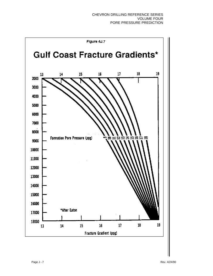
CHEVRON DRILLING REFERENCE SERIESVOLUME FOUR
PORE PRESSURE PREDICTION
Page J - 7 Rev. 4/24/90

CHEVRON DRILLING REFERENCE SERIESVOLUME FOURPORE PRESSURE PREDICTION
Page J - 8 Rev. 4/24/90
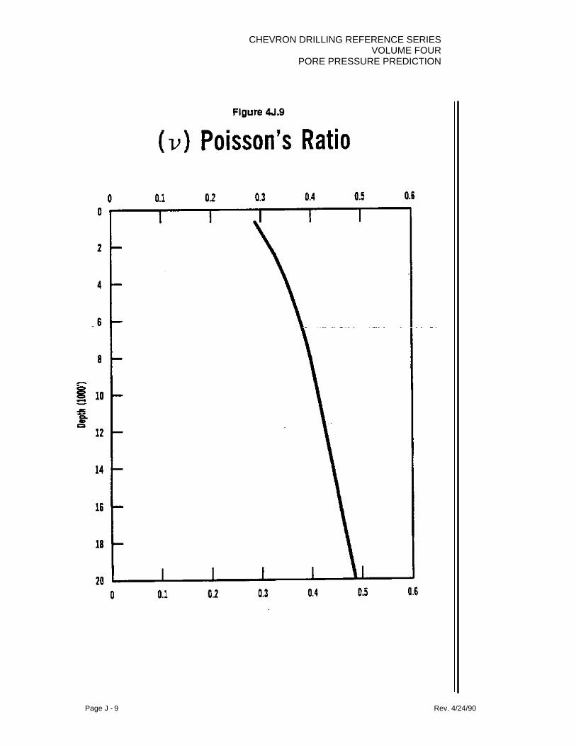
CHEVRON DRILLING REFERENCE SERIESVOLUME FOUR
PORE PRESSURE PREDICTION
Page J - 9 Rev. 4/24/90
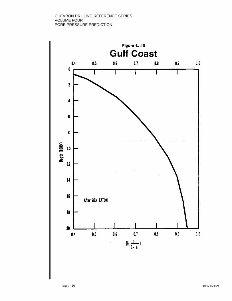
CHEVRON DRILLING REFERENCE SERIESVOLUME FOURPORE PRESSURE PREDICTION
Page J - 10 Rev. 4/24/90
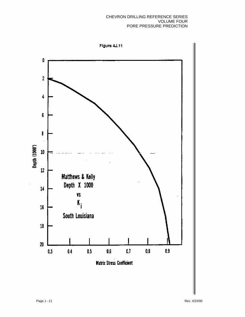
CHEVRON DRILLING REFERENCE SERIESVOLUME FOUR
PORE PRESSURE PREDICTION
Page J - 11 Rev. 4/24/90

CHEVRON DRILLING REFERENCE SERIESVOLUME FOURPORE PRESSURE PREDICTION
Page J - 12 Rev. 4/24/90

CHEVRON DRILLING REFERENCE SERIESVOLUME FOUR
PORE PRESSURE PREDICTION
Page J - 13 Rev. 4/24/90
The matrix stress coefficient, being a function of Poisson’s ratio, varies with depth andthe overburden gradient. Poisson’s ratio for the shallow waters of the Gulf Coast areaappears in Figure 4J.9 The matrix stress coefficients for the same shallow waters of theGulf Coast based on a regionally averaged variable overburden gradient appear in Figure4J.10, as per Ben Eaton. The matrix stress coefficients for the shallow waters of the GulfCoast based on a constant overburden gradient of 1 psi per foot as per Mathews andKelly appears in Figure 4J.11. The regionally averaged variable overburden gradient forthe shallow waters of the Gulf Coast as per Ben Eaton appear in Figure 4J.12.
When we use Eaton’s fracture gradient equation, for a given depth, regardless offormation pore pressure, we plug in a value of matrix stress coefficient for that depth.Theoretically, therefore, the matrix stress coefficient is predominantly dependent on theoverburden gradient. With this in mind, knowing the overburden gradient we might beable to estimate a pseudo-matrix stress coefficient. If we know the overburden gradient,the matrix stress coefficient, and an accurate prediction of formation pore pressure, wecan then estimate the formation fracture gradient.
For example, in Figure 4J.13, we have data for a well drilled in 2130 feet of water.Consider the following, let:
K = G - G G - G
pFma Pma
Oaa Pma
where:K p = pseudo matrix stress coefficientG Fma = the normal fracture gradient for the area for normally pressured rockG Pma = the normal pore pressure gradient for the areaG Oaa = the actual overburden gradient for the area

CHEVRON DRILLING REFERENCE SERIESVOLUME FOURPORE PRESSURE PREDICTION
Page J - 14 Rev. 4/24/90
Figure 4J.13
Green Canyon 114WD ≈≈ 2130 ft
K = G - GG - G
G = G + ( G - G ) K PF P
O P F P O P
nap na
aa na
From the example illustrated, we see from knowing the actual overburden gradient wecan estimate a pseudo matrix stress coefficient. Once estimating a pseudo matrix stresscoefficient, we can utilize it in the Eaton fracture gradient in conjunction with the actualoverburden gradient and estimated pore pressures. Comparing results thus obtained toactual leak off tests for this well in 2130 feet yields excellent results.
Casing Normal Normal Actual ActualShoe Frac F. G. O. BG P. P.TVD M. W. G Fnap G Oaa
4402 14.4 .7488 .605 11.05600 15.0 .7800 .665 12.47100 15.5 .8060 .725 12.69150 16.2 .8424 .775 14.09800 16.4 .8528 .784 14.6
Casing Actual Calc ActualShoe K P PP G G F Frac L. O.TVD G P M.W.
4402 2.0271 .5720 .63890 12.3 12.25600 1.5750 .6448 .67660 13.0 13.47100 1.3115 .6552 .74674 14.4 14.79150 1.2174 .7280 .78520 15.1 15.79800 1.2157 .7592 .78930 15.2 15.6
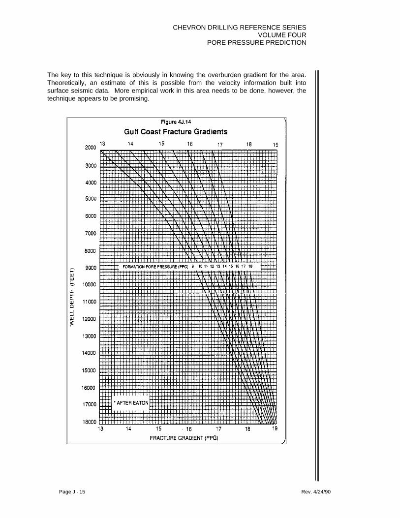
CHEVRON DRILLING REFERENCE SERIESVOLUME FOUR
PORE PRESSURE PREDICTION
Page J - 15 Rev. 4/24/90
The key to this technique is obviously in knowing the overburden gradient for the area.Theoretically, an estimate of this is possible from the velocity information built intosurface seismic data. More empirical work in this area needs to be done, however, thetechnique appears to be promising.

CHEVRON DRILLING REFERENCE SERIESVOLUME FOURPORE PRESSURE PREDICTION
Page J - 16 Rev. 4/24/90

CHEVRON DRILLING REFERENCE SERIESVOLUME FOUR
PORE PRESSURE PREDICTION
Page J - 17 Rev. 4/24/90

CHEVRON DRILLING REFERENCE SERIESVOLUME FOURPORE PRESSURE PREDICTION
Page J - 18 Rev. 4/24/90
Determining Fracture Gradients
Information Required:
1. Pore Pressure plot for the prospective well. 2. Plot of overburden gradient vs. Depth for the area. 3. Plot of matrix stress coefficient for the area. This can be obtained
from Eaton’s plot for the Gulf Coast, from a sonic waveform analysislog run on an offset well, or estimated from leak off test data on otheroffset wells.
PROCEDURE
1. At each inflection point in the pore pressure profile, determine thevalue of the pore pressure gradient (i.e. psi/ft).
2. At the same depth, determine the overburden gradient from theintegrated bulk density log and the matrix stress coefficient from one ofthe sources listed above in #3.
3. Using Eaton’s equation for Fracture gradients, input the values into theequation and determine the fracture gradient (in psi/ft).
4. Convert the fracture gradient into a ppg equivalent by dividing by0.052.

CHEVRON DRILLING REFERENCE SERIESVOLUME FOUR
PORE PRESSURE PREDICTION
Page J - 19 Rev. 4/24/90

CHEVRON DRILLING REFERENCE SERIESVOLUME FOUR
PORE PRESSURE PREDICTION
Page K - 1 Rev. 4/24/90
SECTION K: STUCK PIPE CONSIDERATIONS
1. INTRODUCTION
The occurrence of stuck pipe can significantly increase the cost of drilling, decrease, ifnot eliminate, the success in reaching objectives, and negate attempts to retrievevaluable formation evaluation data. We have developed many tools and techniques inthe oil field to solve problems such as stuck pipe after they occur, but the real key tosavings and success is to avoid problems.
Approximately 600 wells were analyzed throughout the Gulf Coast. This survey includedtrouble-free wells, and those which had experienced differential and mechanical sticking,as well. From this data, we are able to predict the environments which are likely to havea high risk of stuck pipe occurrences. Once knowing the risk factors, we are able toeither design the well to avoid the high risk situations or to plan for it accordingly.
The results of this statistical analysis will be presented in a simple format which enablesone to estimate the risk of stuck pipe occurrence for a given well. Use of the informationfor both well planning and successful execution will be explained and demonstrated.Examples of the occurrence of problems when entering high risk areas will also beillustrated. During the courses of drilling some 100 wells, with attention to the guide linesto be presented, only eight incidences of stuck pipe were encountered.
2. RESULTS OF ANALYSIS
Approximately 600 wells are analyzed in an effort to recognize the environmentconducive to a high risk of stuck pipe occurrence. These wells were drilled over a periodof several years throughout the gulf coast. The statistics were compiled and the resultsof the analysis are presented in a fashion which allows one to estimate the risk of a stuckpipe occurrence in a prescribed well plan scenario.
In Figure 4K.1, we have a curve which estimates the risk of a differential stickingoccurrence. This is for wells drilled as straight holes with water base mud. It assumesformation permeabilities fall within gulf coast average values for any depth. This curvesuggests that when the differential pressure in the wellbore, the differential between themud hydrostatic and the formation pressure, begins to exceed 2000 psi, the probability ofdifferential stuck pipe goes up extremely rapidly. It suggests that differentials muchhigher than 2000 psi should be avoided. Of course, if lower than Gulf Coast averagepermeabilities are expected, then this threshold limit would be higher, and vice versa. Italso assumes that mud properties are not out of line. That is, solids problems, poorrheological characteristics, etc. could result in a lower threshold limit.
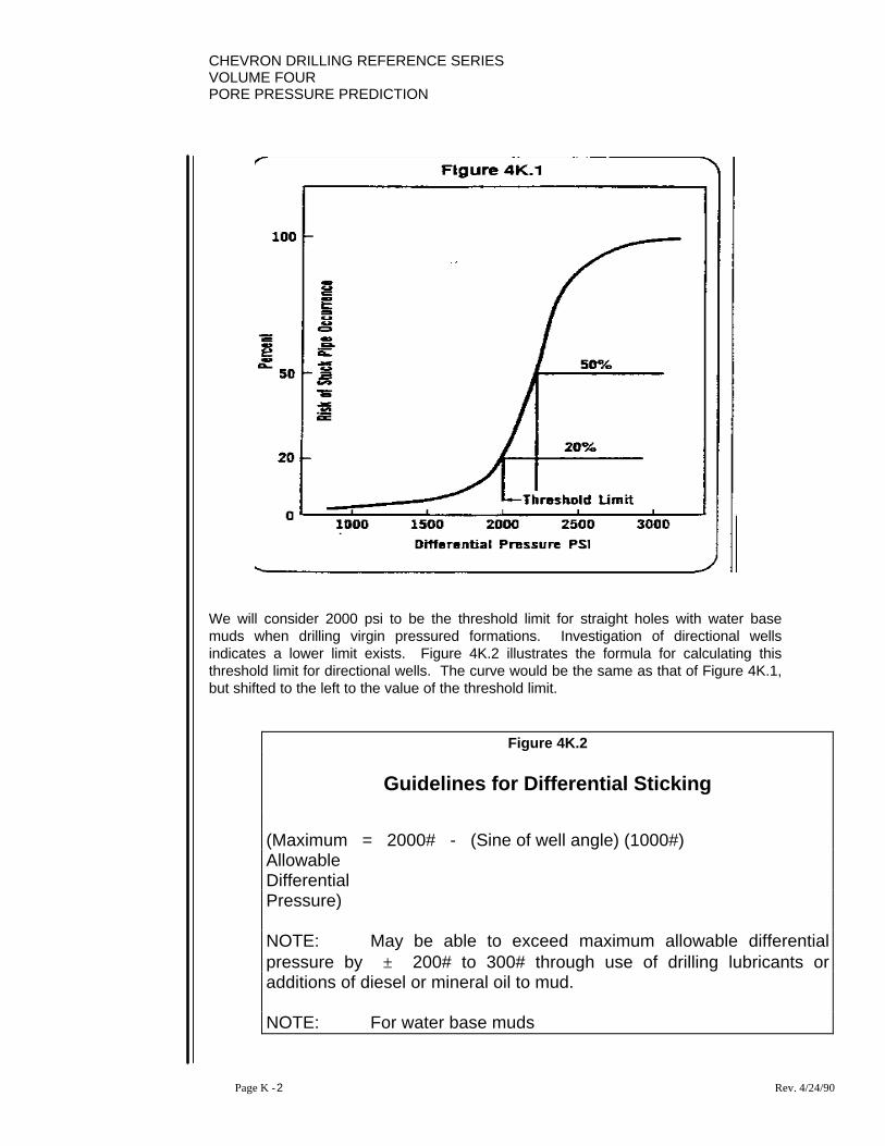
CHEVRON DRILLING REFERENCE SERIESVOLUME FOURPORE PRESSURE PREDICTION
Page K - 2 Rev. 4/24/90
We will consider 2000 psi to be the threshold limit for straight holes with water basemuds when drilling virgin pressured formations. Investigation of directional wellsindicates a lower limit exists. Figure 4K.2 illustrates the formula for calculating thisthreshold limit for directional wells. The curve would be the same as that of Figure 4K.1,but shifted to the left to the value of the threshold limit.
Figure 4K.2
Guidelines for Differential Sticking
(Maximum = 2000# - (Sine of well angle) (1000#)AllowableDifferentialPressure)
NOTE: May be able to exceed maximum allowable differentialpressure by ± 200# to 300# through use of drilling lubricants oradditions of diesel or mineral oil to mud.
NOTE: For water base muds
CHEVRON DRILLING REFERENCE SERIESVOLUME FOUR
PORE PRESSURE PREDICTION
Page K - 3 Rev. 4/24/90
The estimate of the risk of occurrence of mechanically stuck pipe requires a bit moreelaboration. Figure 4K.3 illustrates a general guideline. In the Figure, 95% successmaximum safe angle equates to a scenario which has a 5% risk of a mechanical stuckpipe occurrence. Eighty-five percent success maximum safe angle equates to a scenariowhich has a 15% risk of a mechanical stuck pipe occurrence.
If a well is planned with anticipated mud weight of greater than 14 ppg at total depth, willreach a depth greater than 15,000 feet, and is planned as a 30 degree directional well, ithas a 15% mechanical risk. For wells which are planned with angles greater than the85% success maximum safe angle, calculation of the additional mechanical risk isillustrated in Figure 4K.4. The 85% success angle is subtracted from the magnitude ofthe desired angle to obtain an additional risk angle. The sine of this risk angle multipliedby 200 yields the percent of additional mechanical risk to be expected. Thesemechanical risks can b4e reduced by a reduction of the length of the open hole sectionsby addition of another string of casing to the program. On the surface, this would seemto be a costly addition, however, statistically greater expenditures are made in dealingwith mechanical stuck pipe situations in long open hold sections.

CHEVRON DRILLING REFERENCE SERIESVOLUME FOURPORE PRESSURE PREDICTION
Page K - 4 Rev. 4/24/90
Figure 4K.3
Proposed Directional GuidelinesFor Calculation of Mechanical Risk
Mud Wt. 95% Success 85% SuccessRange Range of Maximum Maximumat TD TD (MD) “Safe” Angle Poss. Angle
9.0 - 10.5 < 10,000’ 50° ± 60°
9.0 - 10.5 10,000’ - 15,000’ 45° ± 60°
9.0 - 10.5 > 15,000’ 40° 45°
10.5 - 12.5 < 10,000’ 45° 55°
10.5 - 12.5 10,000’ - 15,000’ 40° 45°
10.5 - 12.5 > 15,000’ 35° 40°
12.5 - 14.0 < 10,000’ 40° 45°
12.5 - 14.0 10,000’ - 15,000’ 35° 40°
12.5 - 14.0 > 15,000’ 30° 35°
> 14.0 < 10,000’ 35° 40°
> 14.0 10,000’ - 15,000’ 30° 35°
> 14.0 > 15,000’ 25° 30°
• • These guidelines are for the build up and hold angle type directionals• • S-curves are always considered more risky
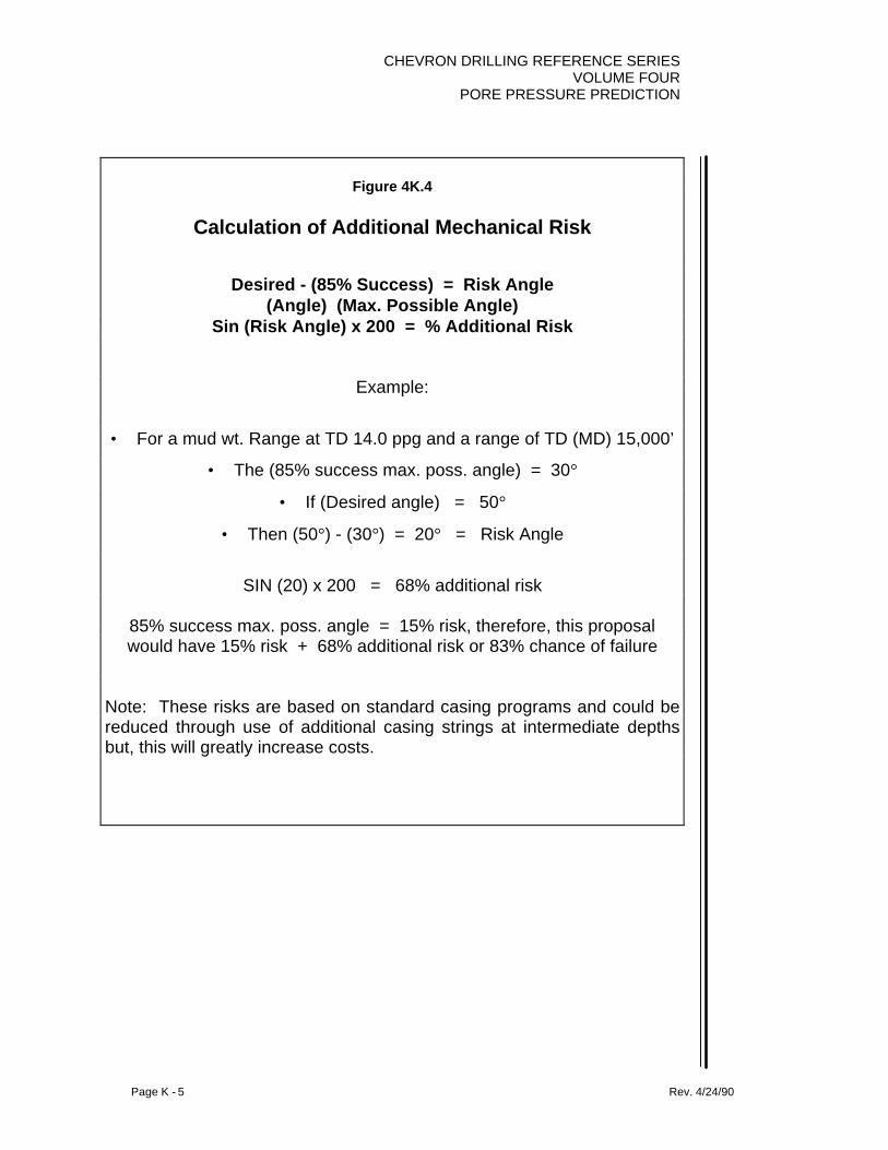
CHEVRON DRILLING REFERENCE SERIESVOLUME FOUR
PORE PRESSURE PREDICTION
Page K - 5 Rev. 4/24/90
Figure 4K.4
Calculation of Additional Mechanical Risk
Desired - (85% Success) = Risk Angle(Angle) (Max. Possible Angle)
Sin (Risk Angle) x 200 = % Additional Risk
Example:
• For a mud wt. Range at TD 14.0 ppg and a range of TD (MD) 15,000’
• The (85% success max. poss. angle) = 30°
• If (Desired angle) = 50°
• Then (50°) - (30°) = 20° = Risk Angle
SIN (20) x 200 = 68% additional risk
85% success max. poss. angle = 15% risk, therefore, this proposalwould have 15% risk + 68% additional risk or 83% chance of failure
Note: These risks are based on standard casing programs and could bereduced through use of additional casing strings at intermediate depthsbut, this will greatly increase costs.

CHEVRON DRILLING REFERENCE SERIESVOLUME FOURPORE PRESSURE PREDICTION
Page K - 6 Rev. 4/24/90
These risk factors are for the build and hold angle type of directional wells. S curve typewells add additional m4echanical risk. We shall define hang down as the length of holebelow the point where the angle begins to drop. The additional risk this drop off presentsis illustrated in Figure 4K.5.
3. HISTORICAL EXAMPLES
In Figure 4K.6, we have a comparison of a proposed casing program vs. That actuallyneeded. The anticipated mud weight at total depth was __ ppg, proposed total measureddepth was 15,558 feet, and the prescribed directional angle 50 degrees. From Figures4K.3 and 4K.4, we calculate a mechanical risk factor of 83% (the example used in Figure4.) During the course of drilling this well, several incidences of mechanically stuck pipewere encountered necessitating costly fishing operations, and an unanticipated additionalstring of intermediate casing in order to reach authorized depth.
Figure 4K.5
Additional Directional Guidelines - S. Curves
Avg. - 4 additional days required to drop angleHangdown = Amount of hole below point where anglebegins to drop
Amount of Hangdown % Risk to Add
≤ 30° drop back to Vertical &Stop
3%
> 30° drop back to Vertical &Stop
5%
≤ 30° 1500’ 8%> 30° 1500’ 10%≤ 30° 2000’ 12%> 30° 2000’ 18%≤ 25° 2500’ 25%> 25° 2500’ 35%3000’ ≥ 50%
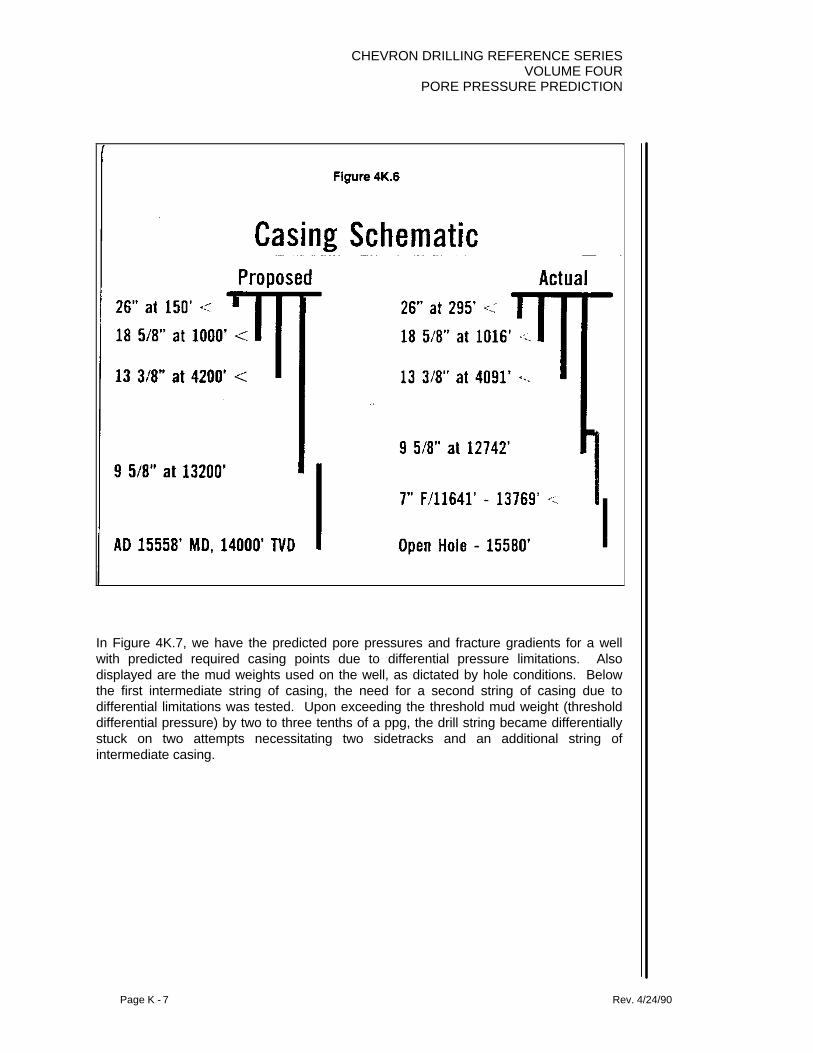
CHEVRON DRILLING REFERENCE SERIESVOLUME FOUR
PORE PRESSURE PREDICTION
Page K - 7 Rev. 4/24/90
In Figure 4K.7, we have the predicted pore pressures and fracture gradients for a wellwith predicted required casing points due to differential pressure limitations. Alsodisplayed are the mud weights used on the well, as dictated by hole conditions. Belowthe first intermediate string of casing, the need for a second string of casing due todifferential limitations was tested. Upon exceeding the threshold mud weight (thresholddifferential pressure) by two to three tenths of a ppg, the drill string became differentiallystuck on two attempts necessitating two sidetracks and an additional string ofintermediate casing.
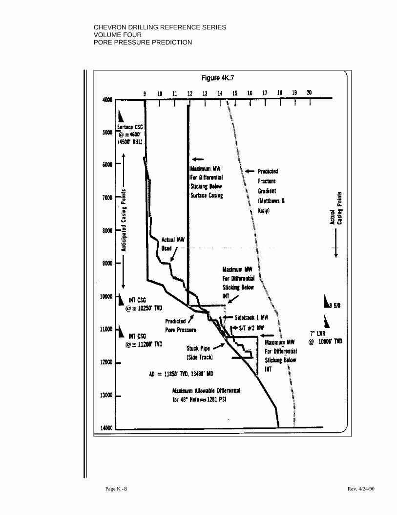
CHEVRON DRILLING REFERENCE SERIESVOLUME FOURPORE PRESSURE PREDICTION
Page K - 8 Rev. 4/24/90

CHEVRON DRILLING REFERENCE SERIESVOLUME FOUR
PORE PRESSURE PREDICTION
Page K - 9 Rev. 4/24/90
4. GENERAL USE IN WELL PLANNING
As a normal course of action in the well planning process, the formation pore pressuresand fracture gradients are predicted. Baring any other considerations, casing pointswould be selected by working down the hole between these two curves as in Figure 4K.8.In this illustration, after setting surface casing, we drill till we reach a point where our porepressures approach within .5 ppg (a safety margin of our anticipated fracture gradient atthe surface casing shoe. We plan to set pipe here and select the next casing point in thesame fashion and so forth. If we analyze further, we examine the anticipated porepressures of all permeable formations exposed in each section of hole and calculate themaximum allowable safe differential pressure we can risk by use of the equation inFigure 4K.2. This determines the maximum mud weight we can afford to exposeformations to and, in turn, to a casing point selection as in Figures 4K.9 and 4K.10.

CHEVRON DRILLING REFERENCE SERIESVOLUME FOURPORE PRESSURE PREDICTION
Page K - 10 Rev. 4/24/90
In consideration of mechanical risks, a similar process is followed. Once again thenormal process of casing point selections would be made as in Figure 4K.8. Once thenormal setting depths are determined, baring any other considerations, we calculate therisk of mechanical sticking using Figures 4K.3 and 4K.4. This has been done in theillustration of Figure 4K.11. Here, we’ve determined the mechanical risk to be 39%. Atthis point, we could eliminate, or reduce this risk by reducing the open hole sectionlengths by the addition of another string of casing to the program, or we may decide thisto be an acceptable risk with which to drill the well.
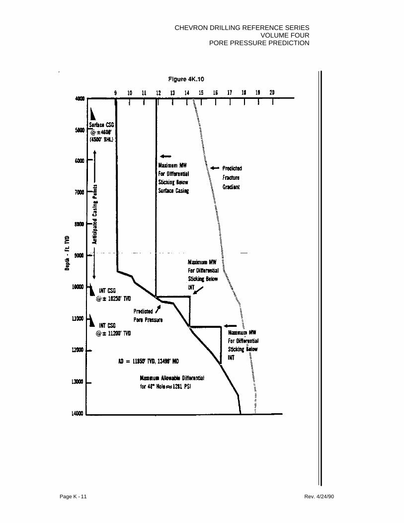
CHEVRON DRILLING REFERENCE SERIESVOLUME FOUR
PORE PRESSURE PREDICTION
Page K - 11 Rev. 4/24/90
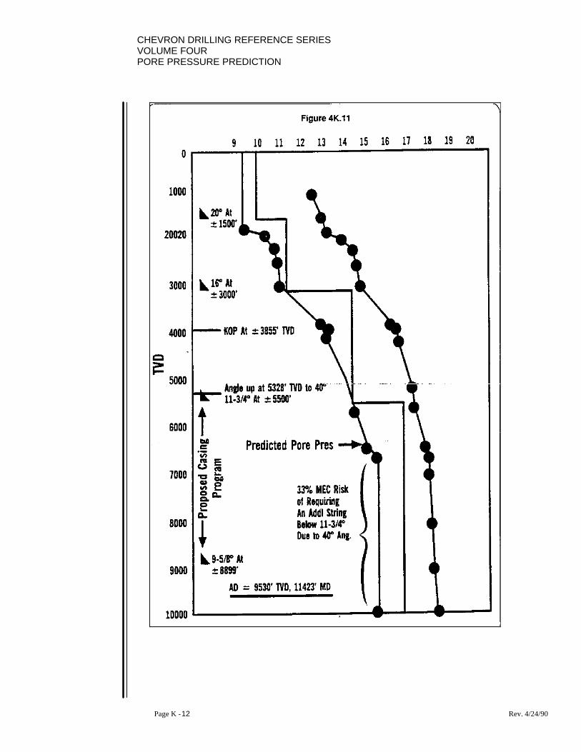
CHEVRON DRILLING REFERENCE SERIESVOLUME FOURPORE PRESSURE PREDICTION
Page K - 12 Rev. 4/24/90

CHEVRON DRILLING REFERENCE SERIESVOLUME FOUR
PORE PRESSURE PREDICTION
Page K - 13 Rev. 4/24/90
5. DIFFERENTIAL PRESSURE AND FAULTS AT CASING POINTS
Once determining anticipated casing points for a proposed well, the occurrence offaulting at these locations presents some interesting problems. In Figure 4K.12, we havea log section. The sand from 13,000 to 13,100 feet is our last normally pressured 9 ppgformation. The next sand seen at 13,350 feet is of a 12.5 ppg pore pressure. As astraight hole, 2000 psi is the differential limitation.
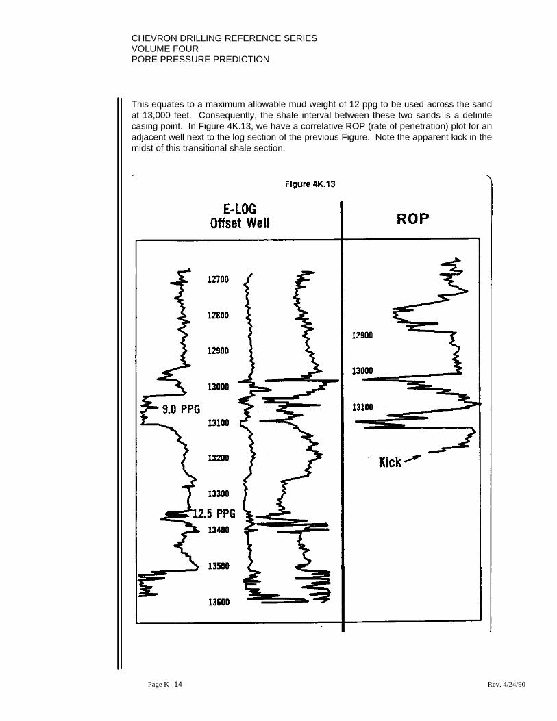
CHEVRON DRILLING REFERENCE SERIESVOLUME FOURPORE PRESSURE PREDICTION
Page K - 14 Rev. 4/24/90
This equates to a maximum allowable mud weight of 12 ppg to be used across the sandat 13,000 feet. Consequently, the shale interval between these two sands is a definitecasing point. In Figure 4K.13, we have a correlative ROP (rate of penetration) plot for anadjacent well next to the log section of the previous Figure. Note the apparent kick in themidst of this transitional shale section.
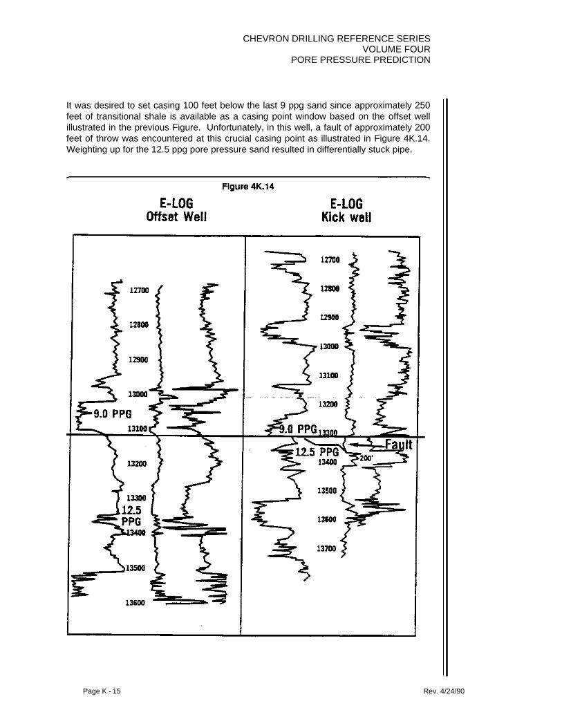
CHEVRON DRILLING REFERENCE SERIESVOLUME FOUR
PORE PRESSURE PREDICTION
Page K - 15 Rev. 4/24/90
It was desired to set casing 100 feet below the last 9 ppg sand since approximately 250feet of transitional shale is available as a casing point window based on the offset wellillustrated in the previous Figure. Unfortunately, in this well, a fault of approximately 200feet of throw was encountered at this crucial casing point as illustrated in Figure 4K.14.Weighting up for the 12.5 ppg pore pressure sand resulted in differentially stuck pipe.
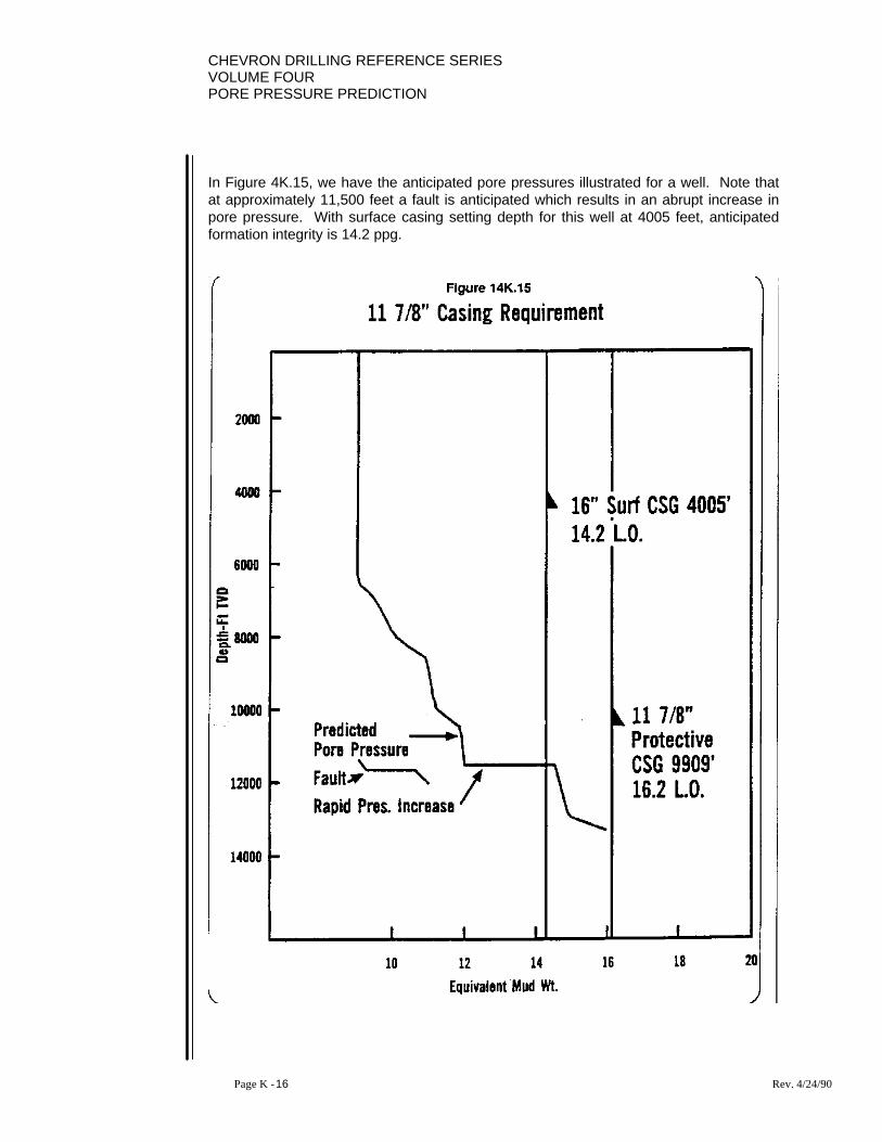
CHEVRON DRILLING REFERENCE SERIESVOLUME FOURPORE PRESSURE PREDICTION
Page K - 16 Rev. 4/24/90
In Figure 4K.15, we have the anticipated pore pressures illustrated for a well. Note thatat approximately 11,500 feet a fault is anticipated which results in an abrupt increase inpore pressure. With surface casing setting depth for this well at 4005 feet, anticipatedformation integrity is 14.2 ppg.

CHEVRON DRILLING REFERENCE SERIESVOLUME FOUR
PORE PRESSURE PREDICTION
Page K - 17 Rev. 4/24/90
Note that upon crossing the fault anticipated, if the first formation seen were to havepermeability, mud weights required to gain well control would exceed the surface casingshoe integrity, a very dangerous situation. Safety considerations require a protectiveintermediate string of casing be set some reasonable distance above the fault to beencountered as illustrat4ed. Plotting the differential pressures which would be seen inthe well due to mud weight requirements results in Figure 4K.16.
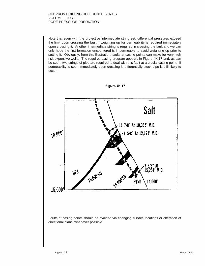
CHEVRON DRILLING REFERENCE SERIESVOLUME FOURPORE PRESSURE PREDICTION
Page K - 18 Rev. 4/24/90
Note that even with the protective intermediate string set, differential pressures exceedthe limit upon crossing the fault if weighting up for permeability is required immediatelyupon crossing it. Another intermediate string is required in crossing the fault and we canonly hope the first formation encountered is impermeable to avoid weighting up prior tosetting it. Obviously, from this illustration, faults at casing points can make for very highrisk expensive wells. The required casing program appears in Figure 4K.17 and, as canbe seen, two strings of pipe are required to deal with this fault at a crucial casing point. Ifpermeability is seen immediately upon crossing it, differentially stuck pipe is still likely tooccur.
Faults at casing points should be avoided via changing surface locations or alteration ofdirectional plans, whenever possible.
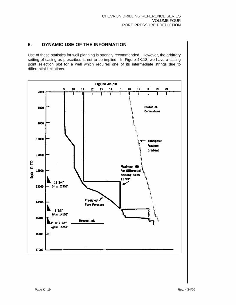
CHEVRON DRILLING REFERENCE SERIESVOLUME FOUR
PORE PRESSURE PREDICTION
Page K - 19 Rev. 4/24/90
6. DYNAMIC USE OF THE INFORMATION
Use of these statistics for well planning is strongly recommended. However, the arbitrarysetting of casing as prescribed is not to be implied. In Figure 4K.18, we have a casingpoint selection plot for a well which requires one of its intermediate strings due todifferential limitations.

CHEVRON DRILLING REFERENCE SERIESVOLUME FOURPORE PRESSURE PREDICTION
Page K - 20 Rev. 4/24/90
The casing program appears in Figure 4K.19 and, as can be seen from the illustration,one string was eliminated during the course of drilling the well.

CHEVRON DRILLING REFERENCE SERIESVOLUME FOUR
PORE PRESSURE PREDICTION
Page K - 21 Rev. 4/24/90
In Figure 4K.20, we have a log section from an offset to this well with a correlative ROPfor the well in question. Note below the 11-3/4” casing string, that the permeable sandsof concern in the offset well from 12,550 to 12,850 feet are shaled-out in our well basedon the ROP plot. If permeable sands are not seen, differential sticking cannot occur.Hence, the mud weight limitation no longer applies. We, therefore, drill beyond thiscasing point based on correlative information gained during the course of drilling the well.

CHEVRON DRILLING REFERENCE SERIESVOLUME FOURPORE PRESSURE PREDICTION
Page K - 22 Rev. 4/24/90
7. ADDITIONAL SIGNIFICANT POINTS
When drilling wells in high pressure environments, there is a tendency to want to pusheach string of casing as deep as possible. Indeed, there are times when this isadvantageous and desirable. However, the pore pressure and fracture gradientpredictions should be studied very closely to determine if this effort is justifiable. Manytimes these efforts are merely costly and inefficient. For example, in Figure 4K.21, wehave illustrated a typical pore pressure and fracture gradient profile of a well. As we lookclosely at this illustration, it can be seen that an intermediate string of casing isnecessary to reach authorized depth in any event.
With an anticipated surface casing shoe test of 14.6 ppg, and a pore pressure at totaldepth of 16 ppg, it is inevitable. The differential limitations of a 9 ppg formation exposedat 12,000 in a straight hole dictates a maximum allowable mud weight of 12.2 ppg. Thiswould dictate a casing point at 12,400 feet. Pushing this string deeper into higherpressure is possible with a surface shoe integrity of 14.6 ppg, however, we riskdifferential sticking needlessly, and very little is gained since the fracture gradient
CHEVRON DRILLING REFERENCE SERIESVOLUME FOUR
PORE PRESSURE PREDICTION
Page K - 23 Rev. 4/24/90
changes little at this intermediate string. We also increase the length and cost of theintermediate string to be run to no advantage. In this example and in many other cases,upon close examination, there are only disadvantages to pushing the intermediate casingstrings beyond the point of the differential pressure limitations.
Application of this information is possible in other parts of the world if we keep in mindthe area for which it was developed in mind, and how it relates geologically to these otherarea. For instance, the differential sticking statistics are based on average Gulf Coastpermeabilities. If we encounter higher permeabilities than this, lower differentialpressures would become a problem and vice versa. Average permeabilities for the GulfCoast appear in Figure 4K.22. Mechanical statistics would have to be related bycomparison of rock composition.
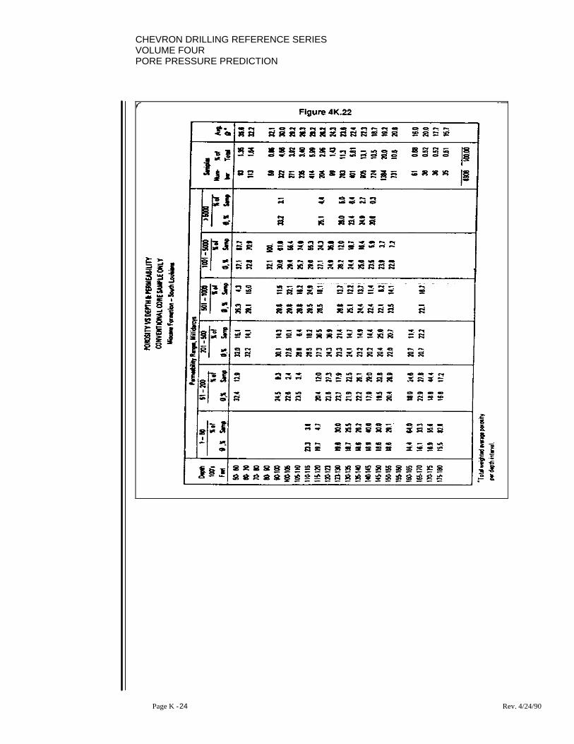
CHEVRON DRILLING REFERENCE SERIESVOLUME FOURPORE PRESSURE PREDICTION
Page K - 24 Rev. 4/24/90

CHEVRON DRILLING REFERENCE SERIESVOLUME FOUR
PORE PRESSURE PREDICTION
Page K - 25 Rev. 4/24/90
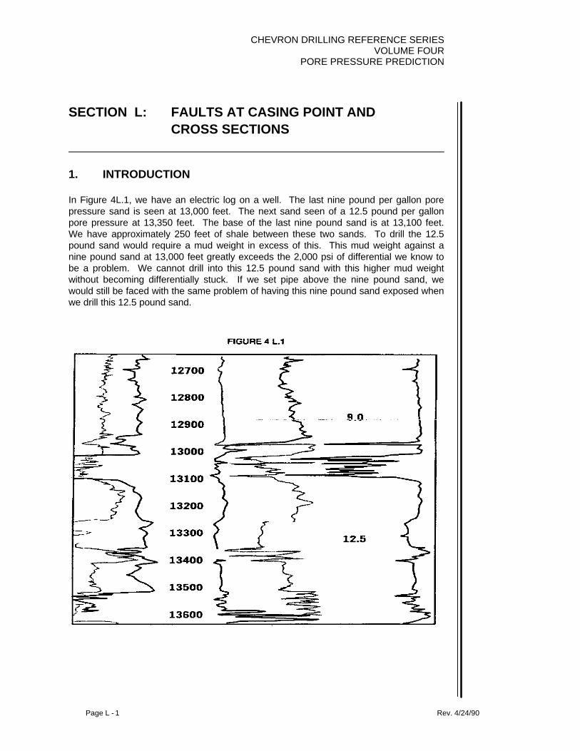
CHEVRON DRILLING REFERENCE SERIESVOLUME FOUR
PORE PRESSURE PREDICTION
Page L - 1 Rev. 4/24/90
SECTION L: FAULTS AT CASING POINT ANDCROSS SECTIONS
1. INTRODUCTION
In Figure 4L.1, we have an electric log on a well. The last nine pound per gallon porepressure sand is seen at 13,000 feet. The next sand seen of a 12.5 pound per gallonpore pressure at 13,350 feet. The base of the last nine pound sand is at 13,100 feet.We have approximately 250 feet of shale between these two sands. To drill the 12.5pound sand would require a mud weight in excess of this. This mud weight against anine pound sand at 13,000 feet greatly exceeds the 2,000 psi of differential we know tobe a problem. We cannot drill into this 12.5 pound sand with this higher mud weightwithout becoming differentially stuck. If we set pipe above the nine pound sand, wewould still be faced with the same problem of having this nine pound sand exposed whenwe drill this 12.5 pound sand.
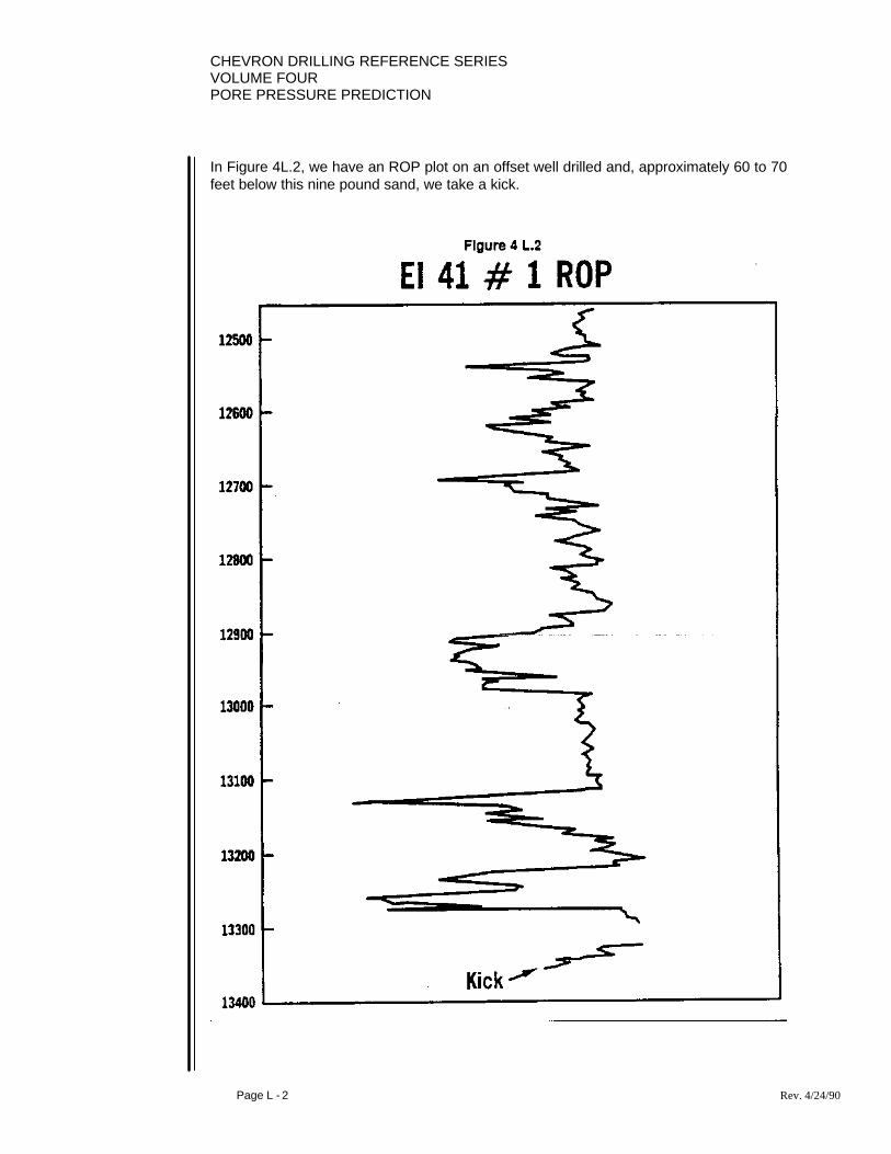
CHEVRON DRILLING REFERENCE SERIESVOLUME FOURPORE PRESSURE PREDICTION
Page L - 2 Rev. 4/24/90
In Figure 4L.2, we have an ROP plot on an offset well drilled and, approximately 60 to 70feet below this nine pound sand, we take a kick.

CHEVRON DRILLING REFERENCE SERIESVOLUME FOUR
PORE PRESSURE PREDICTION
Page L - 3 Rev. 4/24/90
In Figure 4L.3, we have the electric log on the first well on the left and this ROP plot isspliced next to it on the right. The last nine pound sands are correlated together. Basedon correlation, we are taking a kick in the middle of the so-called shale section orwindow.

CHEVRON DRILLING REFERENCE SERIESVOLUME FOURPORE PRESSURE PREDICTION
Page L - 4 Rev. 4/24/90
With logs on both wells side by side, we see in Figure 4L.4 that this shale section, in thewell taking the kick, is no longer 250 feet thick, but rather on the order of 60 feet thick.This is due to a fault encountered in this well faulting out approximately 200 feet of thiswindow, or shale section, bringing this 12.5 pound sand closer to this nine pound sand.$900,000 in expenses were incurred in straightening the situation out on this well.
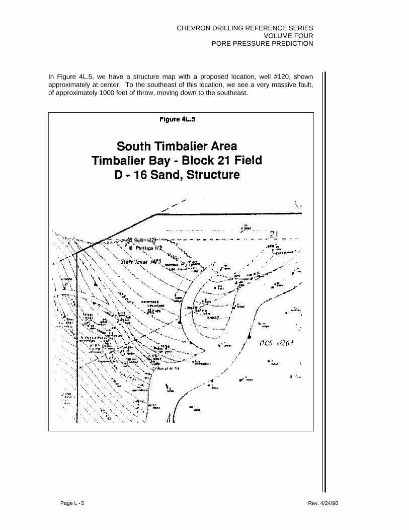
CHEVRON DRILLING REFERENCE SERIESVOLUME FOUR
PORE PRESSURE PREDICTION
Page L - 5 Rev. 4/24/90
In Figure 4L.5, we have a structure map with a proposed location, well #120, shownapproximately at center. To the southeast of this location, we see a very massive fault,of approximately 1000 feet of throw, moving down to the southeast.

CHEVRON DRILLING REFERENCE SERIESVOLUME FOURPORE PRESSURE PREDICTION
Page L - 6 Rev. 4/24/90
We analyze a cross section for this well, Figure 4L.6. The casing window for thisenvironment is between the D10 and D12 sands. We can see along this cross-sectionthat we can be drilling wells where after we come out of the D3 sand, when we cross thefault, the first thing we see could be the D14 sand. The D14 and D16 sands get up in the16 pound range. If all we have set is surface casing and the first thing we see ispermeable sand, we have serious problems. We never know what we will see first whenwe cross a fault. We may be lucky and see some high pressure shale to give usindicators. However, the first thing we see may be a permeable sand in which case wehave extreme difficulties.
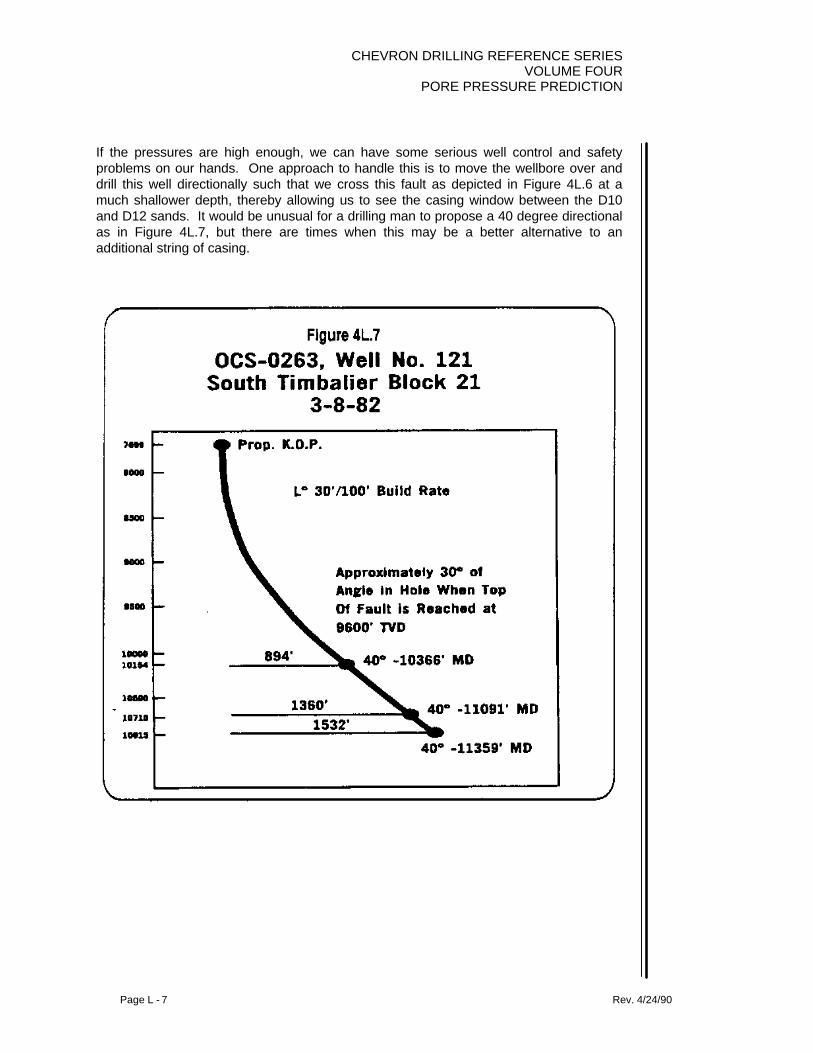
CHEVRON DRILLING REFERENCE SERIESVOLUME FOUR
PORE PRESSURE PREDICTION
Page L - 7 Rev. 4/24/90
If the pressures are high enough, we can have some serious well control and safetyproblems on our hands. One approach to handle this is to move the wellbore over anddrill this well directionally such that we cross this fault as depicted in Figure 4L.6 at amuch shallower depth, thereby allowing us to see the casing window between the D10and D12 sands. It would be unusual for a drilling man to propose a 40 degree directionalas in Figure 4L.7, but there are times when this may be a better alternative to anadditional string of casing.

CHEVRON DRILLING REFERENCE SERIESVOLUME FOURPORE PRESSURE PREDICTION
Page L - 8 Rev. 4/24/90
This is not to say that all faults at casing points are problems. It is a question of whetheror not the magnitude of the throw of the fault significantly exceed or is very close to thecasing window in which we have to set pipe.
In Figure 4L.8, we have a very busy cross section with several faults moving through thearea. We have a series of sands, D7, D8, D9, D10, and then a D11 series. In the caseof this cross-section, the casing window is between the D9 and D11A sands. We see,that even though a fault cuts through this section and faults out the D10 sand, that thereis still several hundred feet of shale between the D9 and D11A sands.
Therefore, a fault at this casing window is not a problem since the throw of the fault issignificantly less than the window in which we have to set pipe. Faults at casing pointsare a problem only if they exceed the window in which we need to set pipe.
In Figure 4L.9, we have a seismic line which passes through a wellbore. We seedepicted a fault moving through the area. This fault was anticipated to have 5000 feet ofthrow. It was also anticipated in the vicinity of our critical casing window. As we analyzethe problem in Figure 4L.10, we see that once we set surface casing, we anticipate a
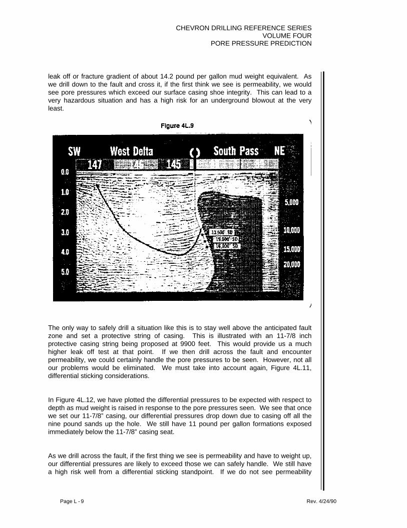
CHEVRON DRILLING REFERENCE SERIESVOLUME FOUR
PORE PRESSURE PREDICTION
Page L - 9 Rev. 4/24/90
leak off or fracture gradient of about 14.2 pound per gallon mud weight equivalent. Aswe drill down to the fault and cross it, if the first think we see is permeability, we wouldsee pore pressures which exceed our surface casing shoe integrity. This can lead to avery hazardous situation and has a high risk for an underground blowout at the veryleast.
The only way to safely drill a situation like this is to stay well above the anticipated faultzone and set a protective string of casing. This is illustrated with an 11-7/8 inchprotective casing string being proposed at 9900 feet. This would provide us a muchhigher leak off test at that point. If we then drill across the fault and encounterpermeability, we could certainly handle the pore pressures to be seen. However, not allour problems would be eliminated. We must take into account again, Figure 4L.11,differential sticking considerations.
In Figure 4L.12, we have plotted the differential pressures to be expected with respect todepth as mud weight is raised in response to the pore pressures seen. We see that oncewe set our 11-7/8” casing, our differential pressures drop down due to casing off all thenine pound sands up the hole. We still have 11 pound per gallon formations exposedimmediately below the 11-7/8” casing seat.
As we drill across the fault, if the first thing we see is permeability and have to weight up,our differential pressures are likely to exceed those we can safely handle. We still havea high risk well from a differential sticking standpoint. If we do not see permeability

CHEVRON DRILLING REFERENCE SERIESVOLUME FOURPORE PRESSURE PREDICTION
Page L - 10 Rev. 4/24/90
immediately, we still have a need for setting another intermediate string of 9-5/8” casing.

CHEVRON DRILLING REFERENCE SERIESVOLUME FOUR
PORE PRESSURE PREDICTION
Page L - 11 Rev. 4/24/90

CHEVRON DRILLING REFERENCE SERIESVOLUME FOURPORE PRESSURE PREDICTION
Page L - 12 Rev. 4/24/90
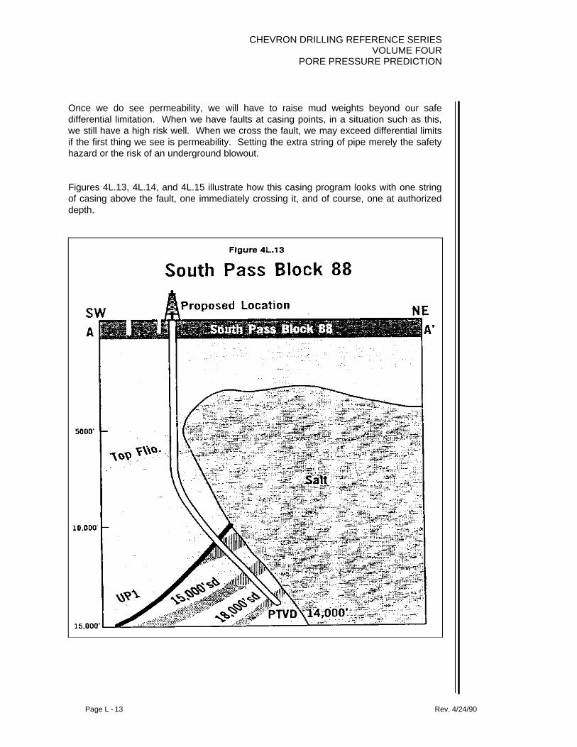
CHEVRON DRILLING REFERENCE SERIESVOLUME FOUR
PORE PRESSURE PREDICTION
Page L - 13 Rev. 4/24/90
Once we do see permeability, we will have to raise mud weights beyond our safedifferential limitation. When we have faults at casing points, in a situation such as this,we still have a high risk well. When we cross the fault, we may exceed differential limitsif the first thing we see is permeability. Setting the extra string of pipe merely the safetyhazard or the risk of an underground blowout.
Figures 4L.13, 4L.14, and 4L.15 illustrate how this casing program looks with one stringof casing above the fault, one immediately crossing it, and of course, one at authorizeddepth.

CHEVRON DRILLING REFERENCE SERIESVOLUME FOURPORE PRESSURE PREDICTION
Page L - 14 Rev. 4/24/90

CHEVRON DRILLING REFERENCE SERIESVOLUME FOUR
PORE PRESSURE PREDICTION
Page L - 15 Rev. 4/24/90
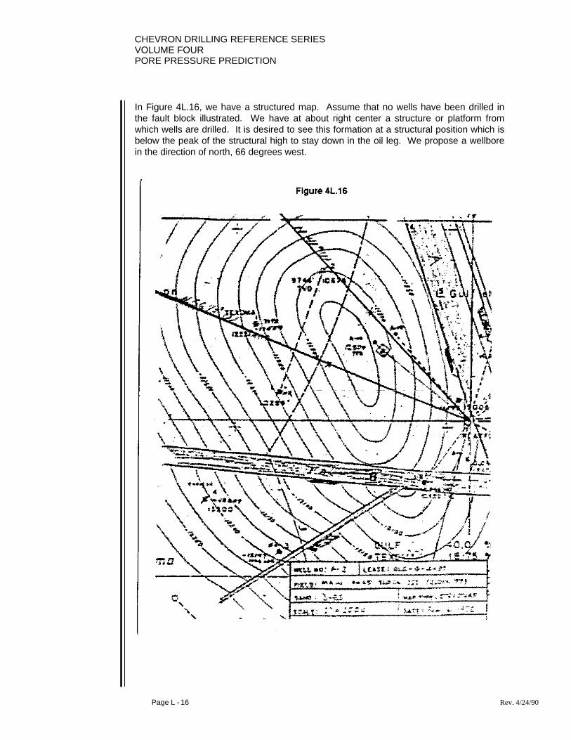
CHEVRON DRILLING REFERENCE SERIESVOLUME FOURPORE PRESSURE PREDICTION
Page L - 16 Rev. 4/24/90
In Figure 4L.16, we have a structured map. Assume that no wells have been drilled inthe fault block illustrated. We have at about right center a structure or platform fromwhich wells are drilled. It is desired to see this formation at a structural position which isbelow the peak of the structural high to stay down in the oil leg. We propose a wellborein the direction of north, 66 degrees west.

CHEVRON DRILLING REFERENCE SERIESVOLUME FOUR
PORE PRESSURE PREDICTION
Page L - 17 Rev. 4/24/90
In Figures 4L.17 and 4L.18, we have 1” log sections on a couple of wells in the areawhich illustrate two things. In Figure 4L.17, we have a transition zone between 9100 feetand 9200 feet where the pore pressure increase from 11.4 ppg to 13.2 ppg. As we lookdeeper, we see a D5 sand which has a 14.5 pore pressure. In Figure 4L.18, we havethis same transition zone between 9300 feet and 9400 feet. We also note additionalsands above the D5 sand in this field such as a D1, D2, and D3 sands.
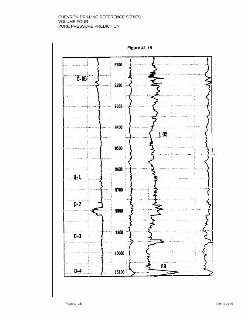
CHEVRON DRILLING REFERENCE SERIESVOLUME FOURPORE PRESSURE PREDICTION
Page L - 18 Rev. 4/24/90

CHEVRON DRILLING REFERENCE SERIESVOLUME FOUR
PORE PRESSURE PREDICTION
Page L - 19 Rev. 4/24/90
Figures 4L.19 through 4L.22 are the fault plane map of the “B” fault, and additionalstructure maps of other formations in the area from which a cross section can be drawn.If we draw a cross section through the proposed plane of North 66 degrees West, we getFigure 4L.23, where we have faulted out our transition zone. We see the D5 sand shortlybelow the cut, but are aware that there are several other possible sands above it, the D1through D4 sands. We could cross this fault and not see our transition zone andencounter permeability first thing.

CHEVRON DRILLING REFERENCE SERIESVOLUME FOURPORE PRESSURE PREDICTION
Page L - 20 Rev. 4/24/90
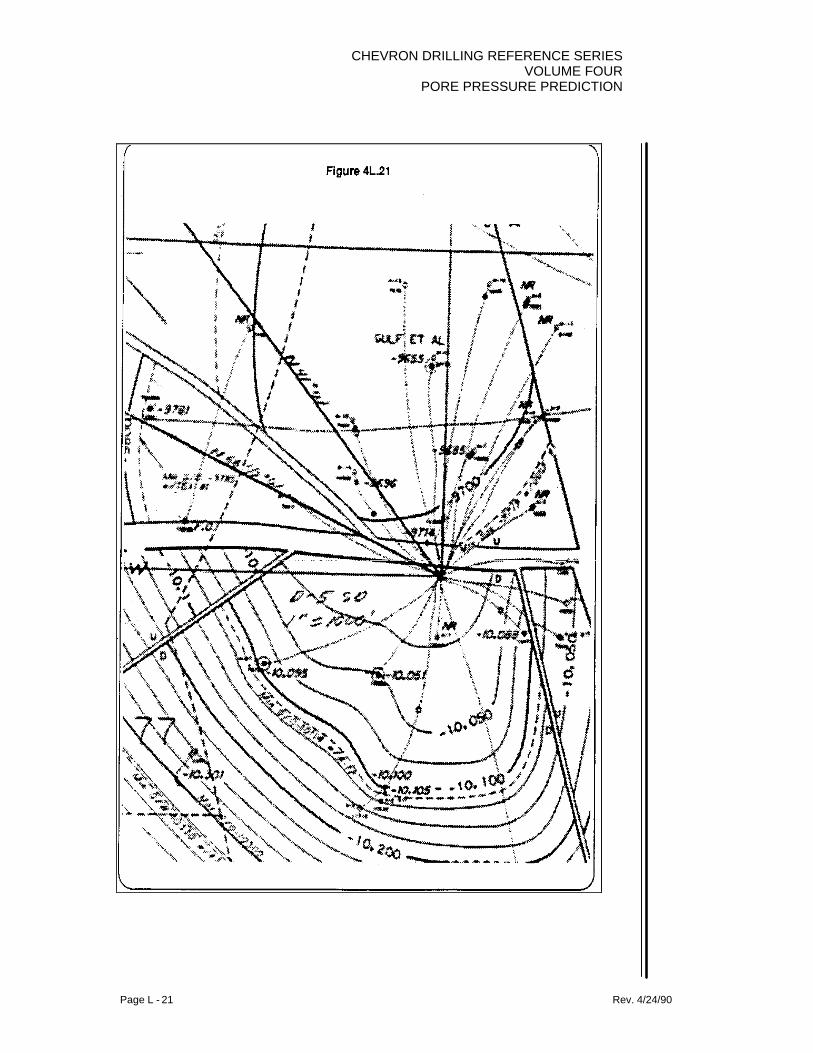
CHEVRON DRILLING REFERENCE SERIESVOLUME FOUR
PORE PRESSURE PREDICTION
Page L - 21 Rev. 4/24/90

CHEVRON DRILLING REFERENCE SERIESVOLUME FOURPORE PRESSURE PREDICTION
Page L - 22 Rev. 4/24/90

CHEVRON DRILLING REFERENCE SERIESVOLUME FOUR
PORE PRESSURE PREDICTION
Page L - 23 Rev. 4/24/90
If we go back to Figure 4L.16, and if satisfied with equal structural position, such asillustrated by the directional heading of North 41 degrees West, we can cut this fault at ashallower depth. As we draw a cross section in this plane, we arrive at Figure 4L.24.We cross the fault at a much shallower depth and we should see the transition zone inthe drilling of our wellbore and can stop the well in this transition zone by moving the faultaway from the critical casing point. This is one of the values of drawing cross sections.Having a cross section through the plane of the well we can see where we anticipatefaults, and what we can do about moving the wellbore or rotating the wellbore to movethat fault away from the casing point. This makes the well much more economical to drilland much safer.
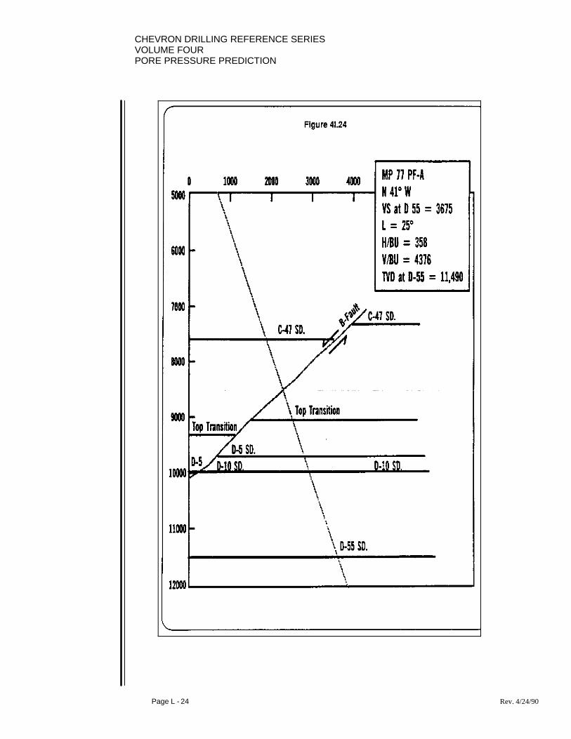
CHEVRON DRILLING REFERENCE SERIESVOLUME FOURPORE PRESSURE PREDICTION
Page L - 24 Rev. 4/24/90

CHEVRON DRILLING REFERENCE SERIESVOLUME FOUR
PORE PRESSURE PREDICTION
Page L - 25 Rev. 4/24/90
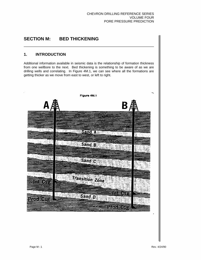
CHEVRON DRILLING REFERENCE SERIESVOLUME FOUR
PORE PRESSURE PREDICTION
Page M - 1 Rev. 4/24/90
SECTION M: BED THICKENING
1. INTRODUCTION
Additional information available in seismic data is the relationship of formation thicknessfrom one wellbore to the next. Bed thickening is something to be aware of as we aredrilling wells and correlating. In Figure 4M.1, we can see where all the formations aregetting thicker as we move from east to west, or left to right.
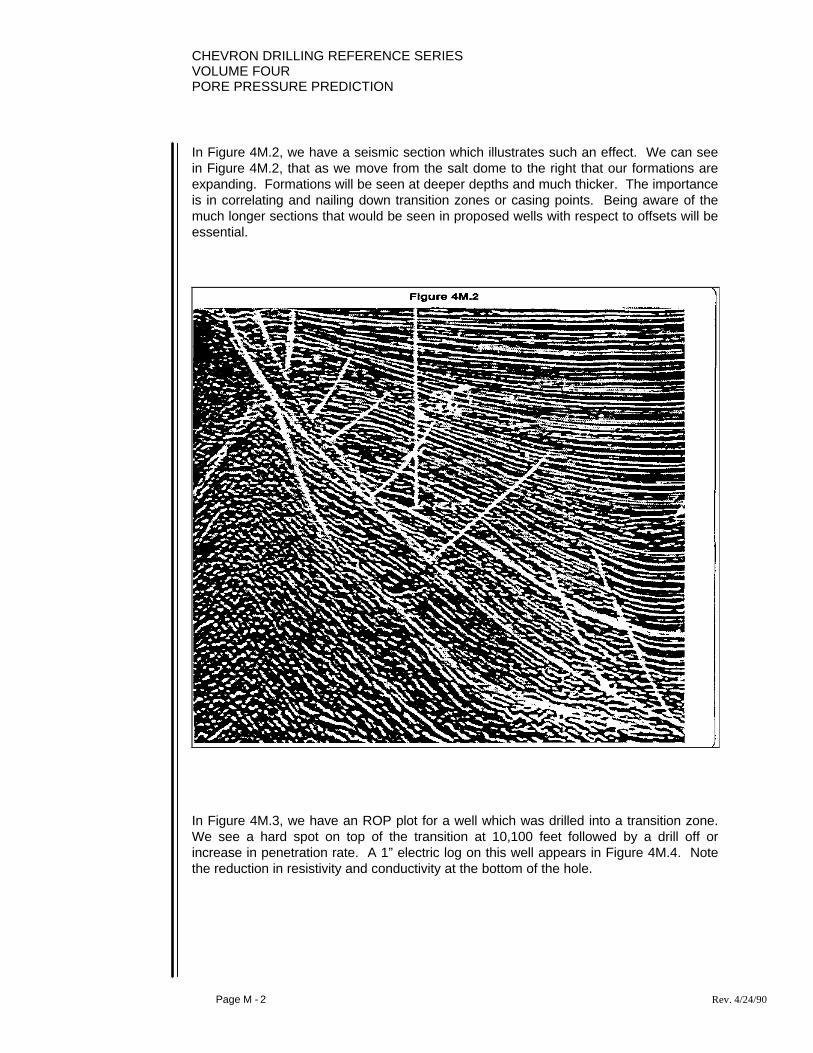
CHEVRON DRILLING REFERENCE SERIESVOLUME FOURPORE PRESSURE PREDICTION
Page M - 2 Rev. 4/24/90
In Figure 4M.2, we have a seismic section which illustrates such an effect. We can seein Figure 4M.2, that as we move from the salt dome to the right that our formations areexpanding. Formations will be seen at deeper depths and much thicker. The importanceis in correlating and nailing down transition zones or casing points. Being aware of themuch longer sections that would be seen in proposed wells with respect to offsets will beessential.
In Figure 4M.3, we have an ROP plot for a well which was drilled into a transition zone.We see a hard spot on top of the transition at 10,100 feet followed by a drill off orincrease in penetration rate. A 1” electric log on this well appears in Figure 4M.4. Notethe reduction in resistivity and conductivity at the bottom of the hole.
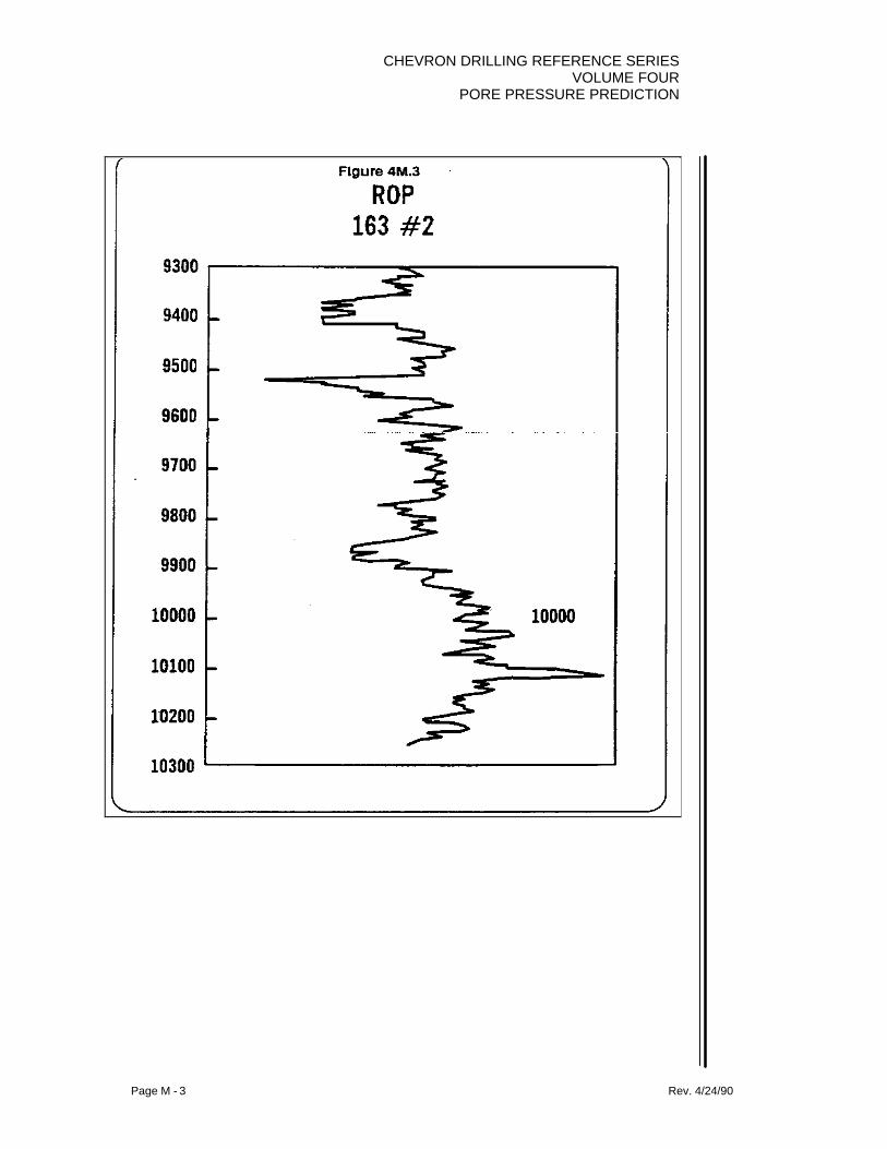
CHEVRON DRILLING REFERENCE SERIESVOLUME FOUR
PORE PRESSURE PREDICTION
Page M - 3 Rev. 4/24/90

CHEVRON DRILLING REFERENCE SERIESVOLUME FOURPORE PRESSURE PREDICTION
Page M - 4 Rev. 4/24/90

CHEVRON DRILLING REFERENCE SERIESVOLUME FOUR
PORE PRESSURE PREDICTION
Page M - 5 Rev. 4/24/90
In Figure 4M.5, we have replaced the conductivity curve with the ROP plot. Note theclose agreement between the two.
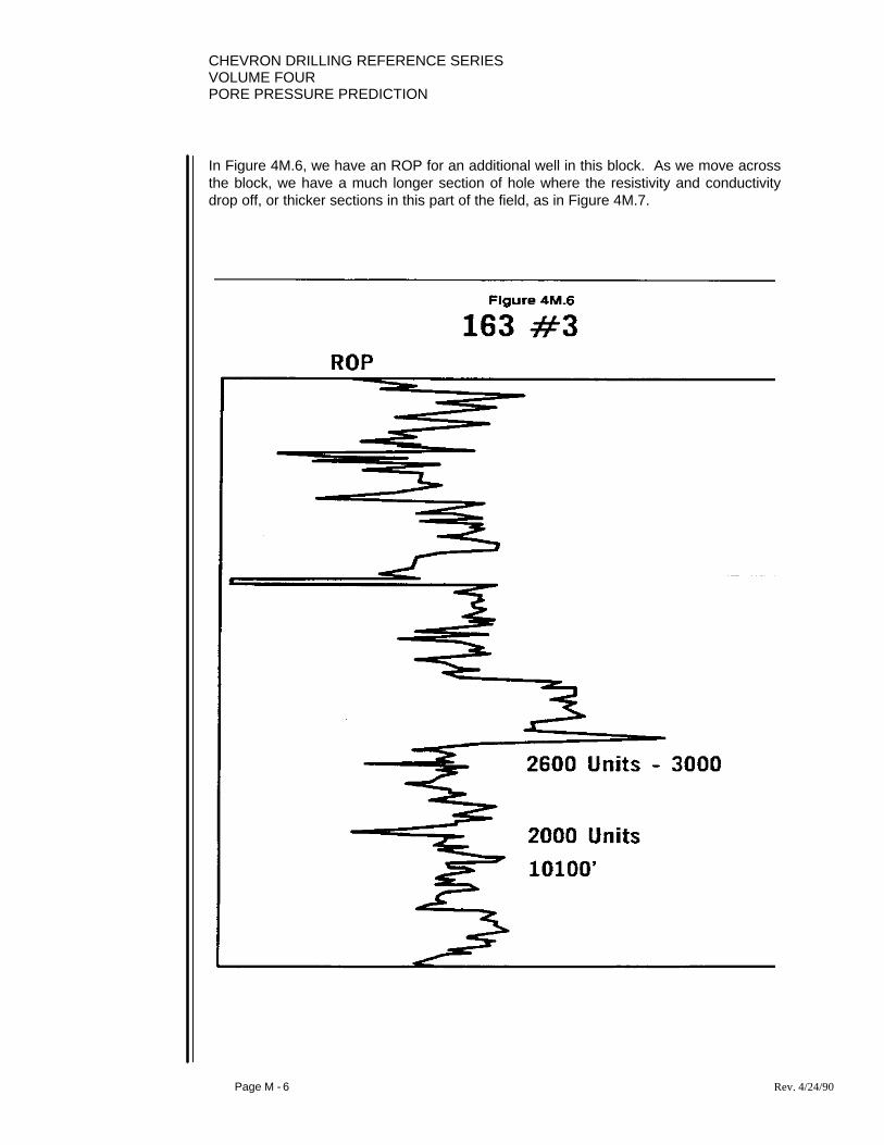
CHEVRON DRILLING REFERENCE SERIESVOLUME FOURPORE PRESSURE PREDICTION
Page M - 6 Rev. 4/24/90
In Figure 4M.6, we have an ROP for an additional well in this block. As we move acrossthe block, we have a much longer section of hole where the resistivity and conductivitydrop off, or thicker sections in this part of the field, as in Figure 4M.7.

CHEVRON DRILLING REFERENCE SERIESVOLUME FOUR
PORE PRESSURE PREDICTION
Page M - 7 Rev. 4/24/90
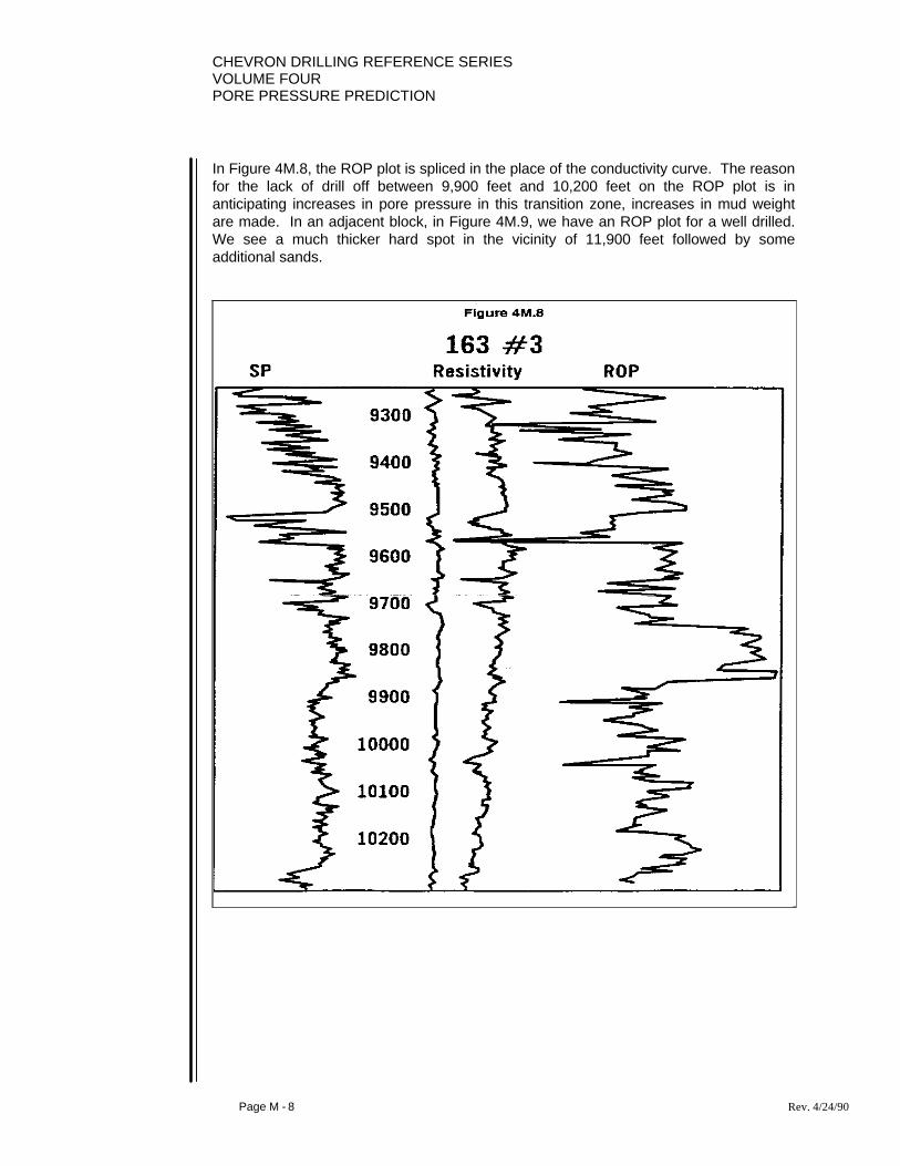
CHEVRON DRILLING REFERENCE SERIESVOLUME FOURPORE PRESSURE PREDICTION
Page M - 8 Rev. 4/24/90
In Figure 4M.8, the ROP plot is spliced in the place of the conductivity curve. The reasonfor the lack of drill off between 9,900 feet and 10,200 feet on the ROP plot is inanticipating increases in pore pressure in this transition zone, increases in mud weightare made. In an adjacent block, in Figure 4M.9, we have an ROP plot for a well drilled.We see a much thicker hard spot in the vicinity of 11,900 feet followed by someadditional sands.

CHEVRON DRILLING REFERENCE SERIESVOLUME FOUR
PORE PRESSURE PREDICTION
Page M - 9 Rev. 4/24/90

CHEVRON DRILLING REFERENCE SERIESVOLUME FOURPORE PRESSURE PREDICTION
Page M - 10 Rev. 4/24/90

CHEVRON DRILLING REFERENCE SERIESVOLUME FOUR
PORE PRESSURE PREDICTION
Page M - 11 Rev. 4/24/90
In Figure 4M.11 appears the ROP plot replacing the conductivity curve next to theelectric log. We see a much thicker hard spot in the vicinity of 9400 feet followed bymuch thicker sands below it.

CHEVRON DRILLING REFERENCE SERIESVOLUME FOURPORE PRESSURE PREDICTION
Page M - 12 Rev. 4/24/90
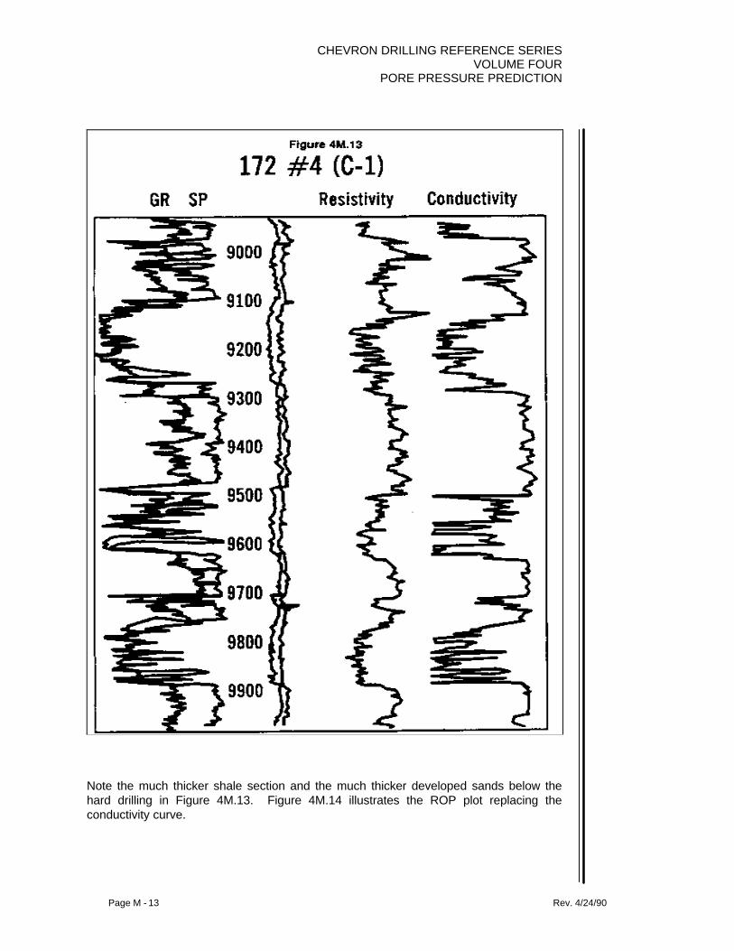
CHEVRON DRILLING REFERENCE SERIESVOLUME FOUR
PORE PRESSURE PREDICTION
Page M - 13 Rev. 4/24/90
Note the much thicker shale section and the much thicker developed sands below thehard drilling in Figure 4M.13. Figure 4M.14 illustrates the ROP plot replacing theconductivity curve.
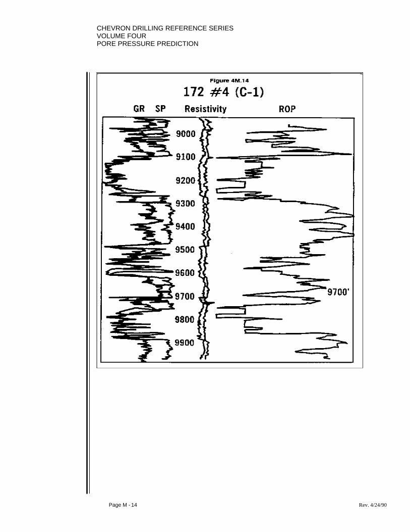
CHEVRON DRILLING REFERENCE SERIESVOLUME FOURPORE PRESSURE PREDICTION
Page M - 14 Rev. 4/24/90
CHEVRON DRILLING REFERENCE SERIESVOLUME FOUR
PORE PRESSURE PREDICTION
Page N - 1 Rev. 4/24/90
SECTION N: CASING POINT SELECTION
1. INTRODUCTION
After building an accurate geological model, consisting of an accurate pore pressure andfracture gradient profile, it is now possible to select optimum, casing setting depths.Considering the fact that the cost of casing and tubing is the greatest tangibleexpenditure related to the overall drilling AFE, it logically follows that the depths to whichthese tubulars are to be set has a major impact on the total well cost. This scenarioobviously points to the need for a sound engineering approach to casing point selection.This section of the Modeling Manual will elaborate on the methodology associated withthis task. It should be kept in mind that even though all wells are not planned anddesigned based on abnormal pore pressure, the building of, and utilization of a modelwill, even in a normal pressured environment, provide clues to potential drilling problems,anticipated wellbore instability areas, and ultimately casing setting depths.
2. GENERAL COMMENTS
The cost effective and optimum selection of casing setting depths is on a fundamentallevel, a delicate balancing act whereby the well planner considers the relationship of aproposed setting point to its pore pressure and fracture gradient environment plus, andonce again relative to a proposed setting point, the development of differential pressureacross any exposed sand, as well as considering mechanical risks. To say all of this in asimpler way, we wish to designate a casing setting depth which does not violateestimated fracture pressure limitations and also does not create a differential pressuremagnitude which increases the probability of differential sticking beyond a reasonablelevel, as well as avoid high mechanical risk situations.
The later two criteria are obviously directly related to four sectors: the drilling fluiddensity in the well at the time of running casing or drilling to the casing point, the truevertical depth of the exposed sands, the estimated permeability of those sands, andfinally the degree of angular inclination projected for the well. To further complicate thisscenario, this model relative to its proposed setting depths is only a tool. The model isalways dynamic; certain wellbore and rig conditions will warrant changes in the proposedsetting point. The expertise required to know when to stop drilling and set pipe, or whento continue drilling to push the point deeper, is not clearly defined by engineering orplanning criteria.
All technology that allows us to accurately determine casing setting point is relative to ourdegree of accuracy in predicting pore pressures and fracture pressures. Time and effortmust be allocated to developing this skill.

CHEVRON DRILLING REFERENCE SERIESVOLUME FOURPORE PRESSURE PREDICTION
Page N - 2 Rev. 4/24/90
3. SURFACE CASING SETTING DEPTHS
Two major considerations will generally control the setting depths of surface casing. Thefirst of these is usually a federal, state or local regulation that will dictate a minimumsetting depth; these regulations are generally related to protecting the shallow sub-surface environment. Exceptions to these regulations may be applied for and obtained.The second consideration in picking surface casing setting depth, is that it should alwaysbe set in a consolidated shale interval when practical. In other words, we should not setsurface easing until we have penetrated sediment where grain-to-grain contact has beenestablished. The grain-to-grain contact will provide a reasonable degree of formationcompetency at the setting depth. This will provide a starting point for determining thedepth at which the intermediate casing can be set without creating a loss circulationproblem.
The estimation or calculation of a formation fracture pressure limitation, thus becomesvery important at the surface setting depth. Under most circumstances, a leak-off test ora pressure integrity test are run shortly after drilling a small amount of new formationbeneath the casing shoe. If executed correctly and consistently, these tests can providea means of quantifying a conservative fracture pressure value and, therefore, will verifyor disqualify the calculated fracture pressure threshold that was utilized in the planningand development phase of the drilling project. Industry experience has definitelyindicated that a wide variety of practices and procedures are employed to successfullyrun leak-off tests.
In addition, the observation and/or evaluation of leak-off test results is highly interpretive,at best. For these reasons, relying solely on field leak-off data to establish a reliablefracture pressure threshold is often a very costly practice. The purpose of this waiting isnot to expound on the short comings of field leak-off values. It suffices to say that at thevery best, the leak-off test values must be considered as tools only. Their applicationrelative to selecting casing points must be evaluated based on experience andconsistency of methodology.
Care must be taken in determining the magnitude of the fracture pressure limitation ofthe surface casing shoe. The value will almost always play at least an indirect role indetermining the intermediate casing setting depth. Occasionally, its magnitude will bethe sole determining factor. Logic should, therefore, indicate that certain circumstanceswill dictate a deepening of the surface casing setting depth in order to achieve a higherformation integrity and, therefore, a greater fracture pressure threshold.
4. INTERMEDIATE CASING SETTING DEPTHS
In general terms, four controlling parameters will interact to determine the safest andmost economical depth at which intermediate casing should be set. Even though thesecontrolling parameters are considered singularly, the final setting depth is the result of a

CHEVRON DRILLING REFERENCE SERIESVOLUME FOUR
PORE PRESSURE PREDICTION
Page N - 3 Rev. 4/24/90
detailed analysis involving all four. Each will be discussed here, followed by a descriptionof this analysis.
As described in the previous section, the magnitude of the fracture pressure, or gradientat the surface casing setting depth will, at least tentatively, provide a threshold drillingfluid density above which the formation at the surface shoe will fracture. The fluid densitythreshold correlates directly with a true vertical depth, as controlled by a plot of porepressure versus depth. This observation is usually the first step in selecting anintermediate casing setting depth, and is considered to be only tentative.
The second parameter to consider is the probability of pipe differential sticking, should infact the previously determined tentative depth be utilized. Experience, and three majorstudies conducted by the MMS and two major oil companies, provide us with differentialsticking guidelines, as previously discussed in this manual.
The tentative intermediate setting depth, that was previously determined relative to theanticipate fracture pressure limitation at the surface casing setting depth, is nowevaluated using the differential pressure criteria. To verbalize the technique, the fluiddensity in which the intermediate casing string well be run is applied across the deepest,normally pressured sand. The differential pressure, given this environment, is calculatedby taking the difference between the drilling fluid density in the well and the pore fluiddensity under normal pressure conditions, in the deepest normally pressured sand. Thisdifference is then multiplied by the pressure gradient constant (0.052) and by the truevertical depth of the sand under consideration.
This product generates a differential pressure magnitude in psi. If the result of thiscalculation is greater than 2000 psi for a straight hole, serious consideration must begiven to raising the tentative intermediate setting point to a shallower depth. Should theabove calculation generate a differential pressure value that is considerable less than2000 psi, from a probability of sticking standpoint, lowering or deepening the tentativeintermediate setting point might be justified. It must be remembered, however, that theinitial setting depth was determined based on the magnitude of the anticipated fracturepressure threshold at the surface casing shoe.
Assuming that this pressure threshold was accurately determined, deepening of theintermediate string, in theory, is not possible. Generally, without violating engineeringprinciples, under these conditions the previously determined intermediate setting depthwould be utilized, or consideration might be given to deepening the surface casing settingdepth, thereby allowing a deeper intermediate setting depth to be chosen. A finalcomment is necessary in relationship to differential sticking considerations. Obviously,as the wellbore inclination departs from the vertical, differential sticking becomes more ofa concern.
After adjusting the intermediate setting depth for differential pressure considerations, thethird parameter is considered. The well is viewed from the proposed intermediate settingpoint to the total depth point. It is then ascertained if the well can be drilled to TD without

CHEVRON DRILLING REFERENCE SERIESVOLUME FOURPORE PRESSURE PREDICTION
Page N - 4 Rev. 4/24/90
setting a second intermediate string of casing. In many cases, the only point ofconsideration for the lower most hole segment is whether or not the fracture pressurelimitation at the intermediate casing shoe is of sufficient magnitude so that it will supportthe maximum drilling fluid density that the well will utilize. However, differential pressurelimitations need be analyzed in this hole segment as well. Should this criteria besatisfied, the previously established intermediate setting depth is sound and the wellshould be drilled below the intermediate shoe to TD without severe problems.
If, however, the fracture pressure threshold at the intermediate casing shoe is notsufficient to support drilling fluid loads to TD, several choices are available. A secondlong intermediate string may be planned to a depth, so that the bottom hold segment canbe drilled safely, or a drilling liner may be set inside of the primary intermediate string.The drilling liner scenario will obviously require design modifications in the primaryintermediate string due to the fact that it will have to support loads generated due todeeper drilling.
One additional option is available which will indirectly allow for deepening of the primaryintermediate string. Under certain circumstance, and assuming compliance with local,state and federal regulations, it may be possible to deepen the setting depth for thesurface casing. Under normal geological development, increasing the depth ofinvestigation will increase the fracture pressure threshold. This increase will allow for adeeper intermediate setting depth which may allow the bottom segment of the well to bedrilled without any major problems related to fracture pressures. It must be rememberedthat differential pressure across the deepest normally pressured sand may still be thecontrolling factor and either limit or negate entirely the possibility of deepening theprimary intermediate casing string.
Finally, mechanical risks need to be evaluated. If an estimation of mechanical risks, aspreviously discussed in this manual, are found to be too high to be acceptable, then areduction in the open hole section lengths via the addition of another string of casingneed be considered. This reduction in open hole lengths will reduce those mechanicalrisks. However, this can add to the overall complexity of the well.
To summarize, intermediate casing setting depth selection involves four basicconsiderations. After calculating and plotting formation pore pressure and fracturepressure, and determining a viable surface casing setting depth relative to previouslydiscussed criteria, the following procedure is followed. A tentative intermediate depth ischosen based on the surface casing shoe’s fracture pressure limitation. The drilling fluiddensity at this tentative depth is then applied as a differential pressure across thedeepest normally pressured sand.
Threshold differential pressures, as previously defined will set the depth limitations. Thetentatively chosen intermediate depth will then be adjusted if needed. After establishingthe adjusted setting depth, the bottom segment of the well below the intermediate settingdepth is examined for drillability relative to drilling fluid density requirements and thefracture pressure threshold at the proposed intermediate casing shoe. Should there not
CHEVRON DRILLING REFERENCE SERIESVOLUME FOUR
PORE PRESSURE PREDICTION
Page N - 5 Rev. 4/24/90
be enough formation integrity at this proposed shoe depth, several scenarios foradditional strings of casing or deepening possibilities must be considered. Finally,adjustments need be evaluated based on mechanical risks.
One additional consideration is sometimes built into the process of selecting anintermediate casing setting depth. This remaining consideration revolves around theconcept of a kick tolerance. The basis for this thinking is predicted on the suppositionthat if a kick is taken when drilling at a given depth, the previous casing shoe must bestrong enough to support that kick. If a kick tolerance is applied in the well planningprocess, it is generally assigned a magnitude of 0.5 ppg, however, careful examination ofkick tolerance may indicate much larger magnitudes and should be seriously considered.
Logic, therefore, implies that utilizing a kick tolerance will have the affect of raising thepreviously determined intermediate setting depth. The specific true vertical depth, asdetermined by utilizing a kick tolerance, is located at that point below which a 0.5 ppgkick would in theory, fracture the previous casing shoe. There again, be reminded thatkick tolerance will be effected by influx volume, open hole length, casing points, etc. Theactual magnitude of the kick is based on the well planner’s prediction of the formationpore pressure plus an 0.5 ppg increase.
Philosophically, this line of thinking proposes that the initial pore pressure prediction wasunsolved. Should the accuracy of the initial geological model (pore pressure prediction)be somewhat suspect, and it is felt that a kick tolerance should be built into the well planas a contingency, it is recommended that an intermediate casing setting depth bedetermined as per normal engineering practices (no kick tolerance), and a shallowerdepth be defined as dictated by the kick tolerance.
Effectively, this well design provides a setting depth window, in which casing can be setwith reasonable assurance of safety and cost effectiveness. It must be remembered thatall well planning work serves only as a guide. Real time analysis of drilling progress andefficiency will either verify the reliability of the planning work, or indicate a need to makemodifications.

CHEVRON DRILLING REFERENCE SERIESVOLUME FOURPORE PRESSURE PREDICTION
Page N - 6 Rev. 4/24/90
It should be apparent that the reliability of pore pressure and fracture pressure predictionis fundamental to optimum casing point selection. Accurate modeling is the key to safedrilling practices, and increasing drilling efficiency.
5. EXAMPLE
The following section described the process of selecting an intermediate casing settingpoint, utilizing a simple example. Figure 4N.2 is the starting point. It illustrates thepredicted formation pore pressure and the predicted formation fracture pressure. Uponexamination of this predictive plot, several points should be noted. Formation porepressure makes a transition from normal (9.0 ppg equivalent in this example) to abnormalat approximately 8000 feet true vertical depth. The pore pressure increases quite rapidlyand continuously until reaching its maximum value of 14.5 ppg equivalent at a truevertical depth of 12,100 feet.
The fracture gradient plot also illustrates an increasing trend. However, as expected, therate of increase in formation integrity is not parallel to that of pore pressure. Theoperating “window” is becoming increasingly smaller with depth.

CHEVRON DRILLING REFERENCE SERIESVOLUME FOUR
PORE PRESSURE PREDICTION
Page N - 7 Rev. 4/24/90
Note that the position of the deepest normally pressured (9.0 ppg equivalent) sand ismarked at 7700 feet true vertical depth.
We may now proceed with the design. The first step is to add a layer of safety margin onthe two predictive curves. This is done first by imposing an over-balanced drilling fluiddensity schedule on the pore pressure estimation, and secondly, by underestimating thepredicted fracture gradient. Typically 0.3 ppg equivalent is used for the fluid densityover-balance, Figure 4N.3, and 0.5 ppg equivalent is used as a safety margin relative tothe predicted fracture pressure, Figure 4N.4 Notice that this has the effect of reducingeven further the operating window. Note that at TD the fluid density will be 15.0 ppg andthe fracture gradient, with design constraints is 17.0 ppg.

CHEVRON DRILLING REFERENCE SERIESVOLUME FOURPORE PRESSURE PREDICTION
Page N - 8 Rev. 4/24/90
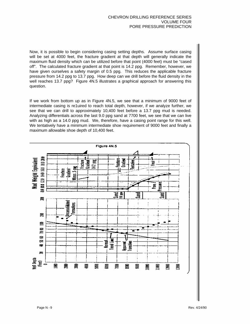
CHEVRON DRILLING REFERENCE SERIESVOLUME FOUR
PORE PRESSURE PREDICTION
Page N - 9 Rev. 4/24/90
Now, it is possible to begin considering casing setting depths. Assume surface casingwill be set at 4000 feet, the fracture gradient at that depth will generally indicate themaximum fluid density which can be utilized before that point (4000 feet) must be “casedoff”. The calculated fracture gradient at that point is 14.2 ppg. Remember, however, wehave given ourselves a safety margin of 0.5 ppg. This reduces the applicable fracturepressure from 14.2 ppg to 13.7 ppg. How deep can we drill before the fluid density in thewell reaches 13.7 ppg? Figure 4N.5 illustrates a graphical approach for answering thisquestion.
If we work from bottom up as in Figure 4N.5, we see that a minimum of 9000 feet ofintermediate casing is re1uired to reach total depth, however, if we analyze further, wesee that we can drill to approximately 10,400 feet before a 13.7 ppg mud is needed.Analyzing differentials across the last 9.0 ppg sand at 7700 feet, we see that we can livewith as high as a 14.0 ppg mud. We, therefore, have a casing point range for this well.We tentatively have a minimum intermediate shoe requirement of 9000 feet and finally amaximum allowable shoe depth of 10,400 feet.
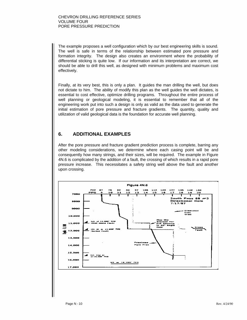
CHEVRON DRILLING REFERENCE SERIESVOLUME FOURPORE PRESSURE PREDICTION
Page N - 10 Rev. 4/24/90
The example proposes a well configuration which by our best engineering skills is sound.The well is safe in terms of the relationship between estimated pore pressure andformation integrity. The design also creates an environment where the probability ofdifferential sticking is quite low. If our information and its interpretation are correct, weshould be able to drill this well, as designed with minimum problems and maximum costeffectively.
Finally, at its very best, this is only a plan. It guides the man drilling the well, but doesnot dictate to him. The ability of modify this plan as the well guides the well dictates, isessential to cost effective, optimize drilling programs. Throughout the entire process ofwell planning or geological modeling, it is essential to remember that all of theengineering work put into such a design is only as valid as the data used to generate theinitial estimation of pore pressure and fracture gradients. The quantity, quality andutilization of valid geological data is the foundation for accurate well planning.
6. ADDITIONAL EXAMPLES
After the pore pressure and fracture gradient prediction process is complete, barring anyother modeling considerations, we determine where each casing point will be andconsequently how many strings, and their sizes, will be required. The example in Figure4N.6 is complicated by the addition of a fault, the crossing of which results in a rapid porepressure increase. This necessitates a safety string well above the fault and anotherupon crossing.

CHEVRON DRILLING REFERENCE SERIESVOLUME FOUR
PORE PRESSURE PREDICTION
Page N - 11 Rev. 4/24/90
In the scenario of Figure 4N.7, three intermediate strings of casing are required.
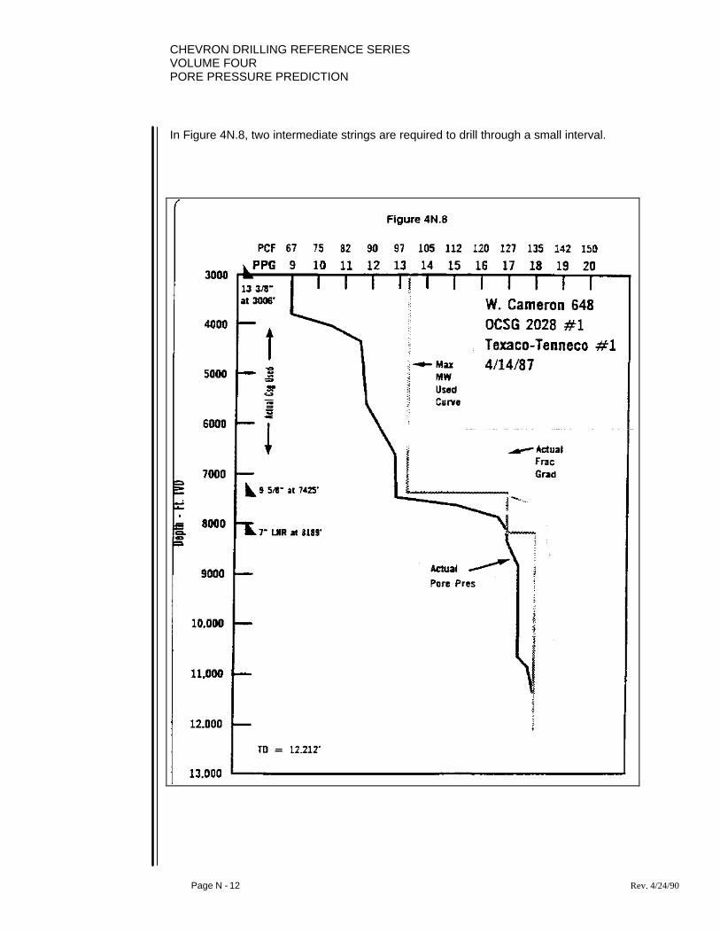
CHEVRON DRILLING REFERENCE SERIESVOLUME FOURPORE PRESSURE PREDICTION
Page N - 12 Rev. 4/24/90
In Figure 4N.8, two intermediate strings are required to drill through a small interval.

CHEVRON DRILLING REFERENCE SERIESVOLUME FOUR
PORE PRESSURE PREDICTION
Page N - 13 Rev. 4/24/90
In the case of Figure 4N.9, its questionable as to the need of the third intermediate soclose to total depth. It would be a logical risk to plan the well without it.
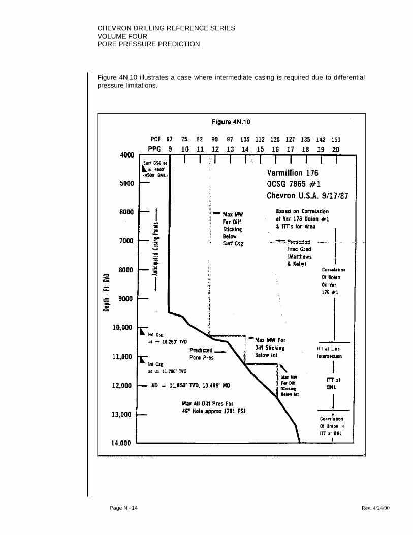
CHEVRON DRILLING REFERENCE SERIESVOLUME FOURPORE PRESSURE PREDICTION
Page N - 14 Rev. 4/24/90
Figure 4N.10 illustrates a case where intermediate casing is required due to differentialpressure limitations.

CHEVRON DRILLING REFERENCE SERIESVOLUME FOUR
PORE PRESSURE PREDICTION
Page N - 15 Rev. 4/24/90
In Figure 4N.11, again, differential pressure is a determining factor in requiring anintermediate casing.

CHEVRON DRILLING REFERENCE SERIESVOLUME FOURPORE PRESSURE PREDICTION
Page N - 16 Rev. 4/24/90
When abnormal pressures are seen to develop at very shallow depth and continue tobuild, many strings of casing can be required to drill in these environments as in Figure4N.12.

CHEVRON DRILLING REFERENCE SERIESVOLUME FOUR
PORE PRESSURE PREDICTION
Page N - 17 Rev. 4/24/90
When pore pressures approach fracture gradients, we approach a point beyond whichwe may not be able to drill as in Figure 4N.13.
The directional considerations of a well are greatly affected by the modeling process. Inthe illustration of Figure 4N.14, if we began to build angle at the prescribed kick off pointof 4450 feet, we would not fully develop our angle until below the next required casingpoint.
It, therefore, becomes necessary to determine the pressures to be seen prior to planningthe directional requirements as in Figure 4N.15. Not only are the directional concernsdependent on the modeling process, but so too are all other drilling considerations.
The second intermediate string in the example of Figure 4N.16, would be required ratherthan attempting to drill a long interval so close to balanced.
In Figure 4N.17, pore pressures do not develop to extremely high magnitudes in thisexample. The selection of the intermediate point should be to minimize differentials ineach hold section.
Missing figures from original notebook!!!
Figure 4N.13
Figure 4N.14
Figure 4N.15
Figure 4N.16
Figure 4N.17

CHEVRON DRILLING REFERENCE SERIESVOLUME FOURPORE PRESSURE PREDICTION
Page N - 18 Rev. 4/24/90
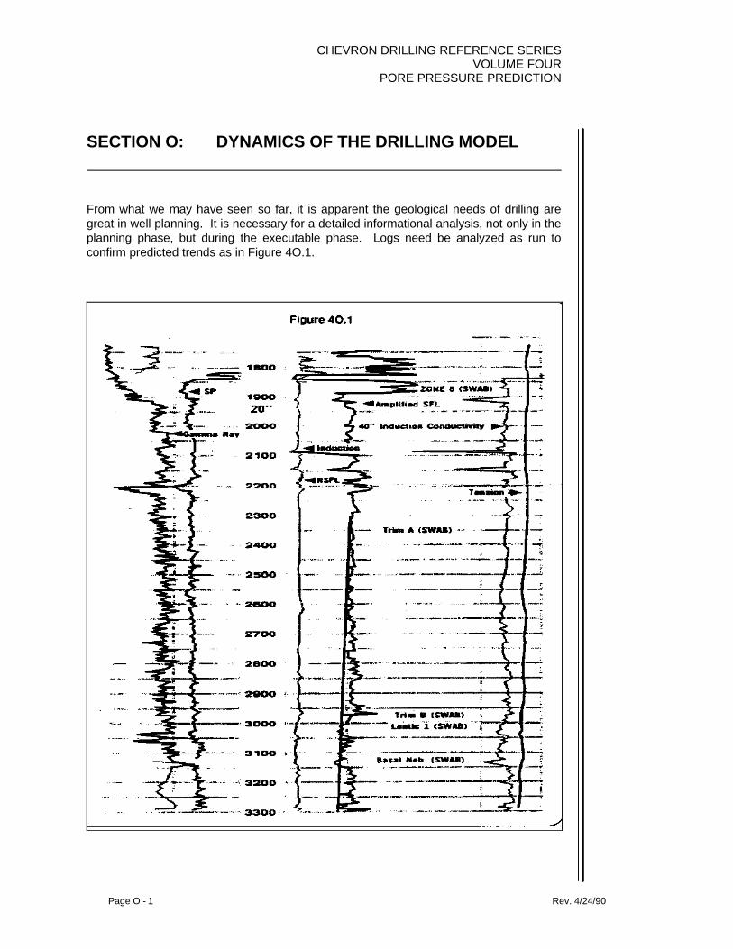
CHEVRON DRILLING REFERENCE SERIESVOLUME FOUR
PORE PRESSURE PREDICTION
Page O - 1 Rev. 4/24/90
SECTION O: DYNAMICS OF THE DRILLING MODEL
From what we may have seen so far, it is apparent the geological needs of drilling aregreat in well planning. It is necessary for a detailed informational analysis, not only in theplanning phase, but during the executable phase. Logs need be analyzed as run toconfirm predicted trends as in Figure 4O.1.

CHEVRON DRILLING REFERENCE SERIESVOLUME FOURPORE PRESSURE PREDICTION
Page O - 2 Rev. 4/24/90
The location of transition zones, as in Figure 4O.2, need to be verified by log analysisprior to running casing.

CHEVRON DRILLING REFERENCE SERIESVOLUME FOUR
PORE PRESSURE PREDICTION
Page O - 3 Rev. 4/24/90
Pore pressures need to be confirmed from log analysis comparisons of normal trends vs.abnormal readings to verify or determine if our anticipations are correct as in Figure4O.3.

CHEVRON DRILLING REFERENCE SERIESVOLUME FOURPORE PRESSURE PREDICTION
Page O - 4 Rev. 4/24/90
Since our initial geological concepts, such as the structure map illustrated in Figure 4O.4,were an interpretation of the available data prior to drilling, as the geologist modifies hisperceptions of the structure from information gathered while drilling, the drilling man needbe aware of modifications which may alter his anticipated formation tops.

CHEVRON DRILLING REFERENCE SERIESVOLUME FOUR
PORE PRESSURE PREDICTION
Page O - 5 Rev. 4/24/90
Anticipated faults, as in Figure 4O.5, may not be encountered or may have a significantlydifferent throw than originally estimated.
Consequently, as new structural information is gained during the course of drilling,proposed casing programs should be modified as in Figure 4O.6, to reflect the effect themoderately changing picture has on drilling parameters.
Figure 4O.6 Missing from original notebook
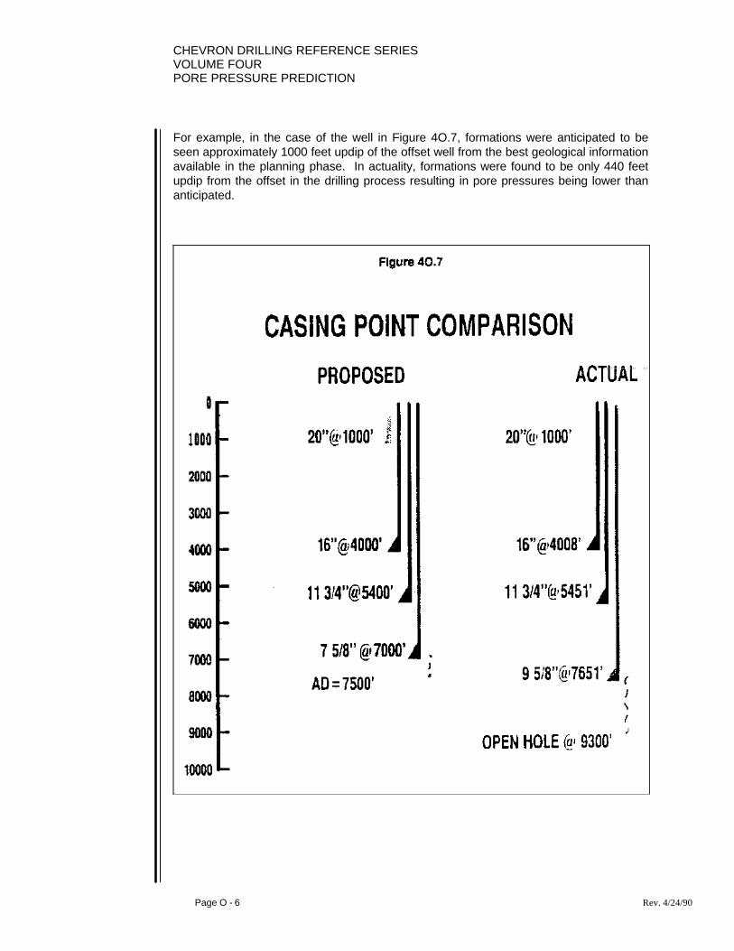
CHEVRON DRILLING REFERENCE SERIESVOLUME FOURPORE PRESSURE PREDICTION
Page O - 6 Rev. 4/24/90
For example, in the case of the well in Figure 4O.7, formations were anticipated to beseen approximately 1000 feet updip of the offset well from the best geological informationavailable in the planning phase. In actuality, formations were found to be only 440 feetupdip from the offset in the drilling process resulting in pore pressures being lower thananticipated.

CHEVRON DRILLING REFERENCE SERIESVOLUME FOURPORE PRESSURE PREDICTION
Page O - 8 Rev. 4/24/90
Figure 4O.8 illustrates another case of modifying the actual casing program during thecourse of drilling from that of the plan. Note the elimination of the second intermediatestring of casing.

CHEVRON DRILLING REFERENCE SERIESVOLUME FOUR
PORE PRESSURE PREDICTION
Page O - 9 Rev. 4/24/90
The need of this second string was based on differential pressure limitations below thefirst intermediate string as illustrated in Figure 4O.9. Permeable sands were anticipatedbelow this string based on the offset wells.

CHEVRON DRILLING REFERENCE SERIESVOLUME FOURPORE PRESSURE PREDICTION
Page O - 10 Rev. 4/24/90
However, during the course of drilling the well, a correlative ROP (rate of penetration)plot, Figure 4O.10 indicates these anticipated sands to be shaled-out between the depthof 12,500 and 12,850 with respect to the offset well.

CHEVRON DRILLING REFERENCE SERIESVOLUME FOUR
PORE PRESSURE PREDICTION
Page O - 11 Rev. 4/24/90
If permeable sands are not exposed, differential sticking cannot occur. Consequently,mud weight limitations can be increased as in Figure 4O.11, which in the case of thiswell, allowed for the elimination of an intermediate string of casing.

CHEVRON DRILLING REFERENCE SERIESVOLUME FOURPORE PRESSURE PREDICTION
Page O - 12 Rev. 4/24/90
In Figure 4O.12, we can see that actual pore pressures encountered were very similar tothose anticipated. So indeed, the lack of the permeable sands was the factor enablingthe elimination of the string.
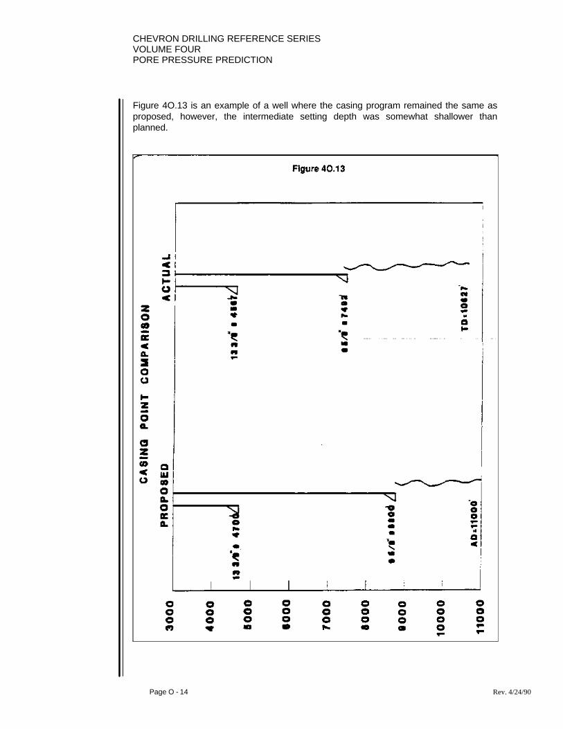
CHEVRON DRILLING REFERENCE SERIESVOLUME FOURPORE PRESSURE PREDICTION
Page O - 14 Rev. 4/24/90
Figure 4O.13 is an example of a well where the casing program remained the same asproposed, however, the intermediate setting depth was somewhat shallower thanplanned.
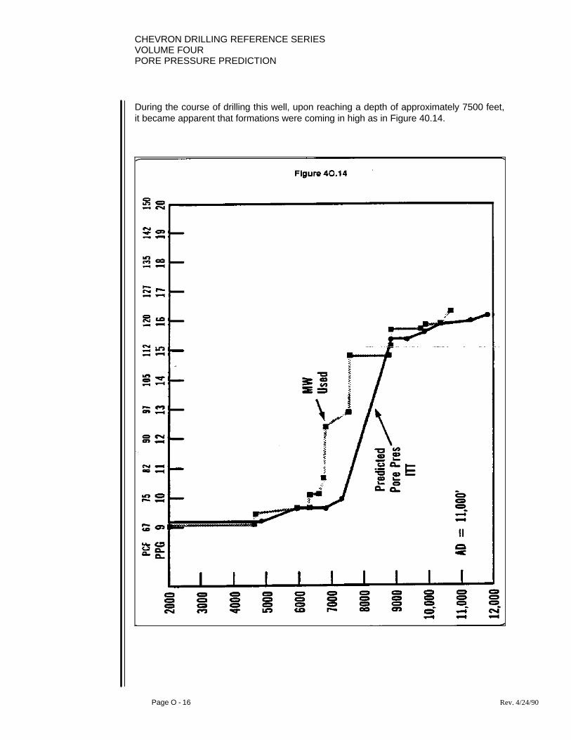
CHEVRON DRILLING REFERENCE SERIESVOLUME FOURPORE PRESSURE PREDICTION
Page O - 16 Rev. 4/24/90
During the course of drilling this well, upon reaching a depth of approximately 7500 feet,it became apparent that formations were coming in high as in Figure 40.14.
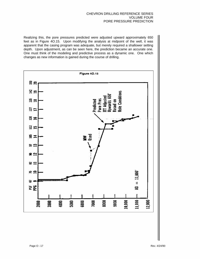
CHEVRON DRILLING REFERENCE SERIESVOLUME FOUR
PORE PRESSURE PREDICTION
Page O - 17 Rev. 4/24/90
Realizing this, the pore pressures predicted were adjusted upward approximately 650feet as in Figure 4O.15. Upon modifying the analysis at midpoint of the well, it wasapparent that the casing program was adequate, but merely required a shallower settingdepth. Upon adjustment, as can be seen here, the prediction became an accurate one.One must think of the modeling and predictive process as a dynamic one. One whichchanges as new information is gained during the course of drilling.

CHEVRON DRILLING REFERENCE SERIESVOLUME FOURPORE PRESSURE PREDICTION
Page O - 18 Rev. 4/24/90

CHEVRON DRILLING REFERENCE SERIESVOLUME FOUR
PORE PRESSURE PREDICTION
Page P - 1 Rev. 4/24/90
SECTION P: THE INTERPRETIVE NATURE OFGEOLOGICAL INFORMATION
The dynamics of the drilling model, or need for modifications, are due to the interpretivenature of the information. The greater the amount and quality of information, the moreaccurate the model, but new information gained during the drilling process always adds anew piece to the puzzle.
Here is an example if the interpretative nature of the geological aspects. Suppose wehave the few bits of information illustrated in Figure 4P.1. We have a fault which runsfrom left to right and three wells which penetrate a given formation at the depthsindicated.

CHEVRON DRILLING REFERENCE SERIESVOLUME FOURPORE PRESSURE PREDICTION
Page P - 2 Rev. 4/24/90
One interpretation of the structure is indicated as one structural high against the fault asin Figure 4P.2.

CHEVRON DRILLING REFERENCE SERIESVOLUME FOUR
PORE PRESSURE PREDICTION
Page P - 3 Rev. 4/24/90
Another, equally valid, interpretation of the same data is with two structural highs againstthe same fault as in Figure 4P.3.
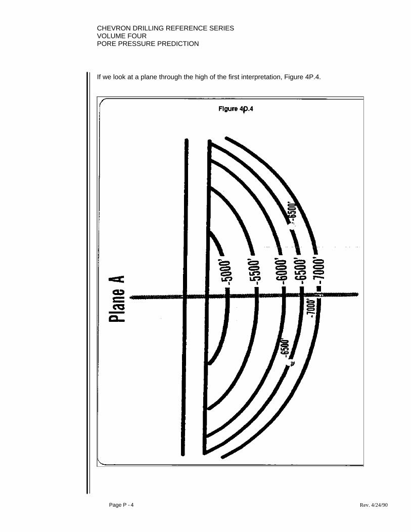
CHEVRON DRILLING REFERENCE SERIESVOLUME FOURPORE PRESSURE PREDICTION
Page P - 4 Rev. 4/24/90
If we look at a plane through the high of the first interpretation, Figure 4P.4.
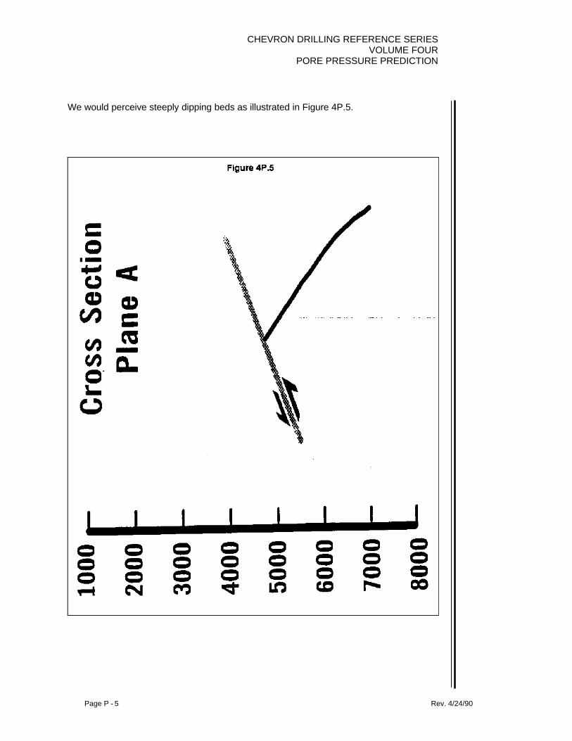
CHEVRON DRILLING REFERENCE SERIESVOLUME FOUR
PORE PRESSURE PREDICTION
Page P - 5 Rev. 4/24/90
We would perceive steeply dipping beds as illustrated in Figure 4P.5.
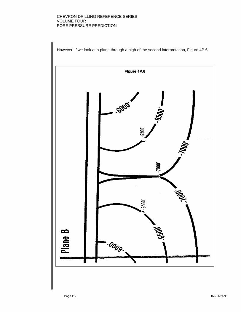
CHEVRON DRILLING REFERENCE SERIESVOLUME FOURPORE PRESSURE PREDICTION
Page P - 6 Rev. 4/24/90
However, if we look at a plane through a high of the second interpretation, Figure 4P.6.

CHEVRON DRILLING REFERENCE SERIESVOLUME FOUR
PORE PRESSURE PREDICTION
Page P - 7 Rev. 4/24/90
We would perceive beds which dip significantly less than before as in Figure 4P.7.

CHEVRON DRILLING REFERENCE SERIESVOLUME FOURPORE PRESSURE PREDICTION
Page P - 8 Rev. 4/24/90

CHEVRON DRILLING REFERENCE SERIESVOLUME FOUR
PORE PRESSURE PREDICTION
Page Q - 1 Rev. 4/24/90
SECTION Q: BASIC GEOLOGICAL CONSIDERATIONS
1. THE BASICS
In Figure 4Q.1, we have a Biostratigraphic Nomenclature Chart for Chevron. This can beutilized to determine geological ages from Chevron paleo data.

CHEVRON DRILLING REFERENCE SERIESVOLUME FOURPORE PRESSURE PREDICTION
Page Q - 2 Rev. 4/24/90
Figure 4Q.2 relates geological time to historical events. Please refer to the followingpages for the Figures.
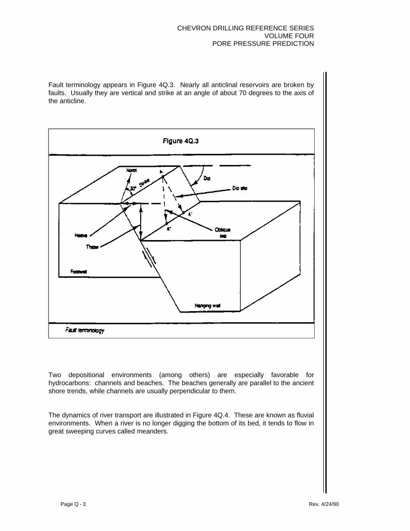
CHEVRON DRILLING REFERENCE SERIESVOLUME FOUR
PORE PRESSURE PREDICTION
Page Q - 3 Rev. 4/24/90
Fault terminology appears in Figure 4Q.3. Nearly all anticlinal reservoirs are broken byfaults. Usually they are vertical and strike at an angle of about 70 degrees to the axis ofthe anticline.
Two depositional environments (among others) are especially favorable forhydrocarbons: channels and beaches. The beaches generally are parallel to the ancientshore trends, while channels are usually perpendicular to them.
The dynamics of river transport are illustrated in Figure 4Q.4. These are known as fluvialenvironments. When a river is no longer digging the bottom of its bed, it tends to flow ingreat sweeping curves called meanders.

CHEVRON DRILLING REFERENCE SERIESVOLUME FOURPORE PRESSURE PREDICTION
Page Q - 4 Rev. 4/24/90
In Figure 4Q.5, appears a diagrammatic cross-section showing the lateral migration ofmeanders. The river is continually undercutting and digging its banks away on theoutside of the meander bends. As a result, the meanders tend to move slowlydownstream. The flood-plain deposits are mostly clay with some silt and sand. The riverpicks up the flood-plain deposits, dropping the sand on the inside of the next bend, butcarrying the clay and silt on downstream. The inside bend, where sand is deposited, iscalled a point bar. The point bars tend to enlarge as the meanders migrate. They maybe buried by later floods and preserved as bodies of clean, porous sand. The reservoirrocks of many oil fields are sandstones deposited as point bar deposits by an ancientriver.
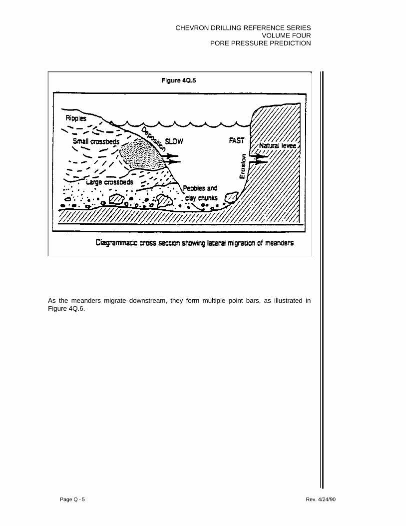
CHEVRON DRILLING REFERENCE SERIESVOLUME FOUR
PORE PRESSURE PREDICTION
Page Q - 5 Rev. 4/24/90
As the meanders migrate downstream, they form multiple point bars, as illustrated inFigure 4Q.6.
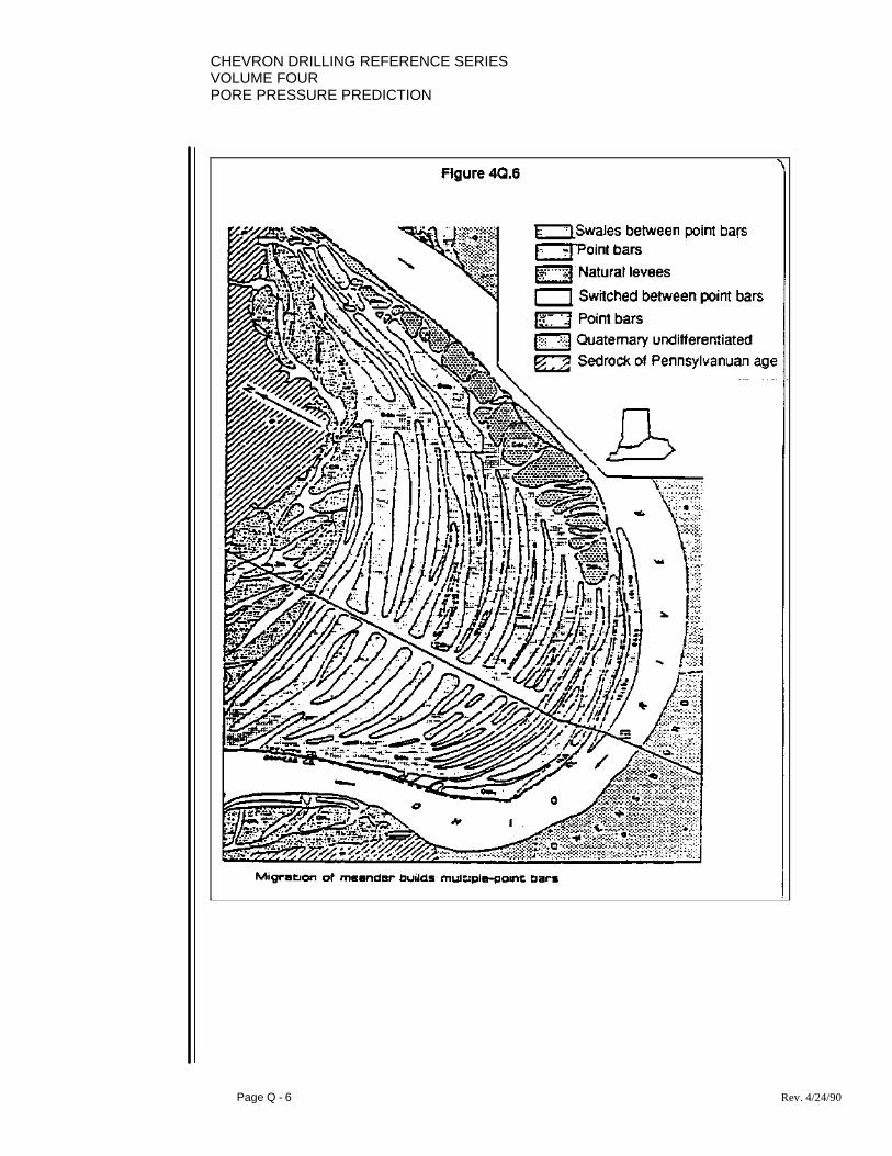
CHEVRON DRILLING REFERENCE SERIESVOLUME FOURPORE PRESSURE PREDICTION
Page Q - 6 Rev. 4/24/90

CHEVRON DRILLING REFERENCE SERIESVOLUME FOUR
PORE PRESSURE PREDICTION
Page Q - 7 Rev. 4/24/90
A typical channel sand deposit is illustrated in Figure 4Q.7. If the river abandons thechannel, as by the cutoff of a meander or upstream diversion, the current finally stopscompletely. Eventually, the abandoned sand-filled channel is buried by flood-plaindeposits.
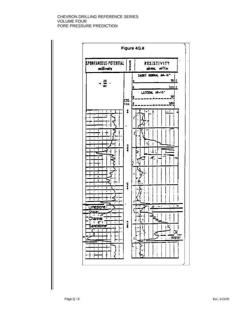
CHEVRON DRILLING REFERENCE SERIESVOLUME FOURPORE PRESSURE PREDICTION
Page Q - 8 Rev. 4/24/90

CHEVRON DRILLING REFERENCE SERIESVOLUME FOUR
PORE PRESSURE PREDICTION
Page Q - 9 Rev. 4/24/90
Channel deposits can be recognized by their erosional base, which truncates olderstratified deposits and causes an abrupt change in lithology to a coarse sand. In thelower part are frequent chunks of clay, apparently pieces of the stream bank which fell in.If these chunks are large enough to exceed the diameter of the wellbore, these sandsmay appear to have shale streaks separating layers of sand or as vertical permeabilitybarriers on an electric log. Vertical permeability may exist, however, beyond thewellbore.
Channel sands can often be recognized on the electric log using the gamma-ray SP, andshort-spacing resistivity curves. The base is abrupt. Usually, both SP and resistivity area maximum in the lower layer because the sand contains less clay and has a higherporosity. The overlying beds contain more clay, both interstitial and in laminae, so bothSP and resistivity decrease in amplitude and become serrated near the top.
The electric log response of a channel sandstone appears in Figure 4Q.8. Water velocityin stream channels varies, and when it is reduced, causes setting of the heaviest andlargest components first. Continued reduction of velocity causes progressively finematerials to be deposited over the coarse beds. Typical electric-log response to channelsands indicates an increase in SP in the bottom of a channel sand, which canoccasionally imply increased permeability. Knowing the environment to be that ofchannel sands should imply anticipation of differential sticking to be more likely at thebase of the sands than at the top due to the increasing permeability as we drill throughthe sand. If the hole is acting sticky at the top of the sand, differential sticking is likely atthe base and vice versa.
A typical beach or barrier bar sand appears in Figure 4Q.9. The waves of the oceancontinually strike the shore. At the front of a delta, the waves winnow the clay from thesand, building up a beach of clean sand. Such beaches are often buried by layers ofmud as the delta builds outward. They thus become completely enclosed in shale andform stratigraphic traps for oil. The rush of the waves and along-shore currents smoothout the coastline so that beaches and barrier islands are often nearly straight. Behindthe barrier island is a quiet lagoon where both sand and mud are deposited. The grainsize and cleanness of the sand thus decrease away from the ocean toward the land.Thus, as we head inward from the beach area, significant reductions in permeability canbe expected.
An electric log response of a beach deposit appears in Figure 4Q.10. Electric logresponse of beach deposits is the inverse of that for stream channel sands. Beachsands are deposited upon fine-grained sediments that have little porosity and reducedSP and resistivity response. Therefore, permeabilities are likely to be higher at the topwith a gradual reduction as we reach the base. If differential sticking is not a problem atthe top of the sand, it is not likely to occur as we drill deeper to the base.

CHEVRON DRILLING REFERENCE SERIESVOLUME FOURPORE PRESSURE PREDICTION
Page Q - 10 Rev. 4/24/90

CHEVRON DRILLING REFERENCE SERIESVOLUME FOUR
PORE PRESSURE PREDICTION
Page Q - 11 Rev. 4/24/90
In Figure 4Q.11 we have a diagrammatic cross-section of a typical channel sand body.Chunks of shale several inches to several feet in diameter are often found near the sidesof the sand body. These are pieces of the stream banks that caved in when the currentundercut them. The bedding often shows festoon crossbeds that dip in the downstreamdirectional of the current. These are the internal characteristics of a channel. Becauseof these large cavings, correlations can sometimes be difficult or misleading from well towell. One well may see the sand as nice clean body while another may appear to haveseveral sands separated by shale layers.
A typical beach-type sand appears in Figure 4Q.12. Beaches and barrier-island sandbodies have the cleanest and coarsest sand in the upper part, where it is most washedby the waves. The sand is often stirred up by burrowing organisms such as clams. Theseaward pinch-out is abrupt, smooth, and straight. The landward side toward the lagoontends to be transitional, the sands becoming dirty and inter-fingering with the shale(muds) of the lagoon. The lagoon side is irregular. As we head seaward, toward thepinch-out, the sands thin and permeabilities decline. If differential sticking is not aproblem in the vicinity of the beach, it becomes less likely as we head farther toward thesea.

CHEVRON DRILLING REFERENCE SERIESVOLUME FOURPORE PRESSURE PREDICTION
Page Q - 12 Rev. 4/24/90
A summary of electric log patterns of sand bodies of different environments appears inFigure 4Q.13. The alluvial-fan and braided-stream deposits show as stacks of sand withthin shale beds. The point bars nearly always show the abrupt base and narrow top (bellshale), while the stream-mouth and barrier bars show the broad, abrupt top andgradational base (funnel shape). The turbidities show stacked sand bodies separated byshale beds.

CHEVRON DRILLING REFERENCE SERIESVOLUME FOUR
PORE PRESSURE PREDICTION
Page Q - 13 Rev. 4/24/90
Some typical representations of sphericity and roundness in sand grains appear in Figure4Q.14.

CHEVRON DRILLING REFERENCE SERIESVOLUME FOURPORE PRESSURE PREDICTION
Page Q - 14 Rev. 4/24/90
Some of the basic terminology and structure of clay minerals appears in Figure 4Q.15.There are four principal types of clay minerals. The kaolinites consist of one silicatetrahedral layer and one alumina octahedral layer linked together. They adsorb wateronly around the edges, not between the layers; they do not swell. The chemicalcomposition of kaolinite is (OH)8Al4Si4O10.
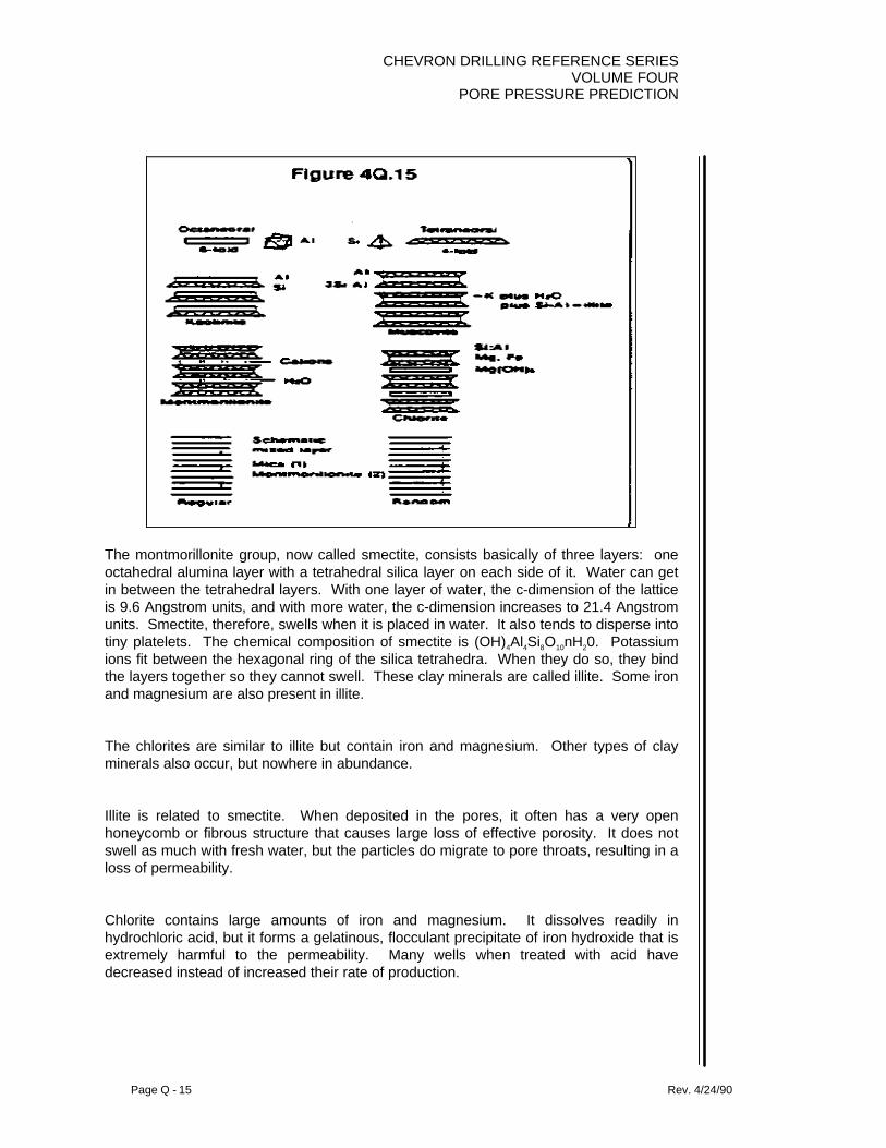
CHEVRON DRILLING REFERENCE SERIESVOLUME FOUR
PORE PRESSURE PREDICTION
Page Q - 15 Rev. 4/24/90
The montmorillonite group, now called smectite, consists basically of three layers: oneoctahedral alumina layer with a tetrahedral silica layer on each side of it. Water can getin between the tetrahedral layers. With one layer of water, the c-dimension of the latticeis 9.6 Angstrom units, and with more water, the c-dimension increases to 21.4 Angstromunits. Smectite, therefore, swells when it is placed in water. It also tends to disperse intotiny platelets. The chemical composition of smectite is (OH)4Al4Si8O10nH20. Potassiumions fit between the hexagonal ring of the silica tetrahedra. When they do so, they bindthe layers together so they cannot swell. These clay minerals are called illite. Some ironand magnesium are also present in illite.
The chlorites are similar to illite but contain iron and magnesium. Other types of clayminerals also occur, but nowhere in abundance.
Illite is related to smectite. When deposited in the pores, it often has a very openhoneycomb or fibrous structure that causes large loss of effective porosity. It does notswell as much with fresh water, but the particles do migrate to pore throats, resulting in aloss of permeability.
Chlorite contains large amounts of iron and magnesium. It dissolves readily inhydrochloric acid, but it forms a gelatinous, flocculant precipitate of iron hydroxide that isextremely harmful to the permeability. Many wells when treated with acid havedecreased instead of increased their rate of production.
CHEVRON DRILLING REFERENCE SERIESVOLUME FOURPORE PRESSURE PREDICTION
Page Q - 16 Rev. 4/24/90
There are certain effects of drilling mud on sandstone to be considered. When drillingover-balanced, a filter cake develops on the face of a permeable sandstone. In order tominimize invasion of mud and mud filtrate, steps are taken to decrease the permeabilityof the filter cake. Most of the solids in the mud remain in the filter cake and do not enterthe sand pores. However, a small amount of fine particles does enter and tends to plugthe pores in the vicinity of the wellbore.
The filtrate from the drilling mud enters the sand and often invades it for a distance ofseveral feet. If the sand contains swelling clays, they may originally have beenflocculated in the salty, connate pore water. When this is displaced by fresh water,swelling occurs. Certain chemicals put in the drilling mud to reduce its water loss willdeflocculate the clays in the pores. Even if there is no swelling, the flow of water maypick up and move the delicate authigenic clay particles, causing blocking.
If there is oil in the rock, the water may form stable emulsions or asphalt films that blockthe pores. If the chemicals in the drilling mud react with the compounds in the pore waterto form precipitates, these will also cause blocking. The surfactants in the mud maycause the oil to be displaced so completely that the permeability of the sand to oil isgreatly decreased.
A typical mud filter cake permeability appears in Figure 4Q.16.
A comparative illustration of permeability grain size and shape appear in Figure 4Q.17.Grains oriented in one direction can increase rock permeability parallel to their long axesand reduce it normal to their long axes. This is particularly true where small, flat shalegrains provide no permeability normal to the fissility of the shale, but can allow the lateralmovement of fluids along it during compaction.
Figure 4Q.16
PERMEABILITY OF MUD FILTER CAKE = 10-3 MD
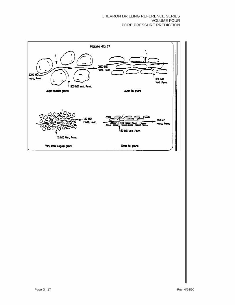
CHEVRON DRILLING REFERENCE SERIESVOLUME FOUR
PORE PRESSURE PREDICTION
Page Q - 17 Rev. 4/24/90

CHEVRON DRILLING REFERENCE SERIESVOLUME FOURPORE PRESSURE PREDICTION
Page Q - 18 Rev. 4/24/90
A generalized classification of problem shales appears in Figure 4Q.18.
Figure 4Q.18
CLASSIFICATION OF PROBLEM SHALES
CLASS CHARACTERISTICS CLAY CONTENT
1 Soft, high dispersion High in montmorillonite, someillite
2 Soft, fairly high dispersion Fairly high in montmorillonite,high in illite
3 Medium hard, moderatedispersion, sloughing tendencies
High in inter-layered clays, highin illite, chlorite
4 Hard, little dispersion, sloughingtendencies
Moderate illite, moderate chlorite
5 Very hard, brittle, no significantdispersion, caving tendencies
High in illite, moderate chlorite
An abundant sedimentary rock that often contains oil is limestone. Sometimes thelimestone contains substantial amount of magnesium, replacing calcium, and it thenbecomes dolomite. It has become customary in the oil business to call both limestoneand dolomite carbonates to avoid making a distinction.
It has been estimated that about half the world’s oil reserves are in carbonates, althoughthere are numerically fewer carbonate than sandstone reservoirs outside the Middle East.
Carbonates differ in many respects from sandstones. They are mostly formed from theremains of animals (shellfish) and plants (algae); they are, therefore, found in nearly thesame place where they originated and were not transported and then deposited likesandstones.
Typical limestone nomenclature appears in Figure 4Q.19. A carbonate rock consists ofthree textural components: grains, matrix, and cement. The cement is clear calcite thatfilled or partially filled the pores after the original deposition. There are several differentkinds of grains, of which four are the most important. These are (1) shell fragments,called “bio”; (2) fragments of previously deposited limestones, called “intraciasts”; (3)small round pellets, the excreta of worms and other small burrowing organisms; and (4)ooliths, spheres formed by rolling and coating lime particles along the bottom.

CHEVRON DRILLING REFERENCE SERIESVOLUME FOUR
PORE PRESSURE PREDICTION
Page Q - 19 Rev. 4/24/90
The matrix is lime of clay-particle size (lime mud). It is called micrite. The clearsecondary calcite cement is called sparite.Thus, a rock consisting mainly of clear secondary calcite with intraclast grains would becalled “intrasparite”. A rock consisting mainly of micrite (lime mud) with grains consistingof broken shell fragments would be called “biomicrite”. Biomicrite and pelmicrite are themost common limestone types. These eight types are shown diagrammatically in Figure4Q.19.
Besides these eight combinations, there are some limestones consisting only of micriteand some consisting of the remains of upstanding reef-building organisms. So there areten types of limestones in all.
The types of grains typically seen in limestones appear in Figure 4Q.20. The type ofgrains is considered significant. Five types of grains: detrital “intraclasts”; skeletal “bio”;pellets “pellets”; lumps (irregular clumps; and coated grains “ooliths”.
The carbonate depositional environment and characteristic rock types appear in Figure4Q.21. Many, if not most, ancient carbonates were deposited simultaneously in threedifferent macro-environments - shelf, slope, and basin.
Shelf
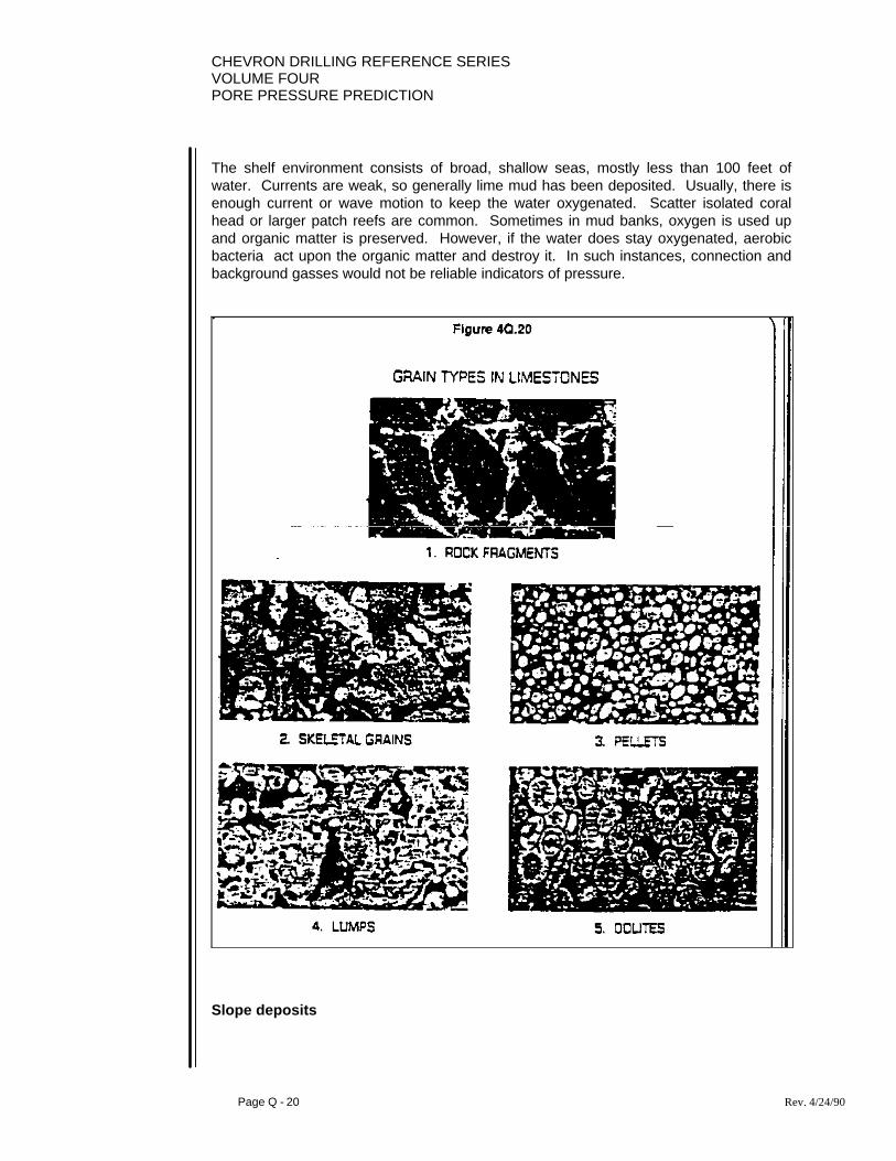
CHEVRON DRILLING REFERENCE SERIESVOLUME FOURPORE PRESSURE PREDICTION
Page Q - 20 Rev. 4/24/90
The shelf environment consists of broad, shallow seas, mostly less than 100 feet ofwater. Currents are weak, so generally lime mud has been deposited. Usually, there isenough current or wave motion to keep the water oxygenated. Scatter isolated coralhead or larger patch reefs are common. Sometimes in mud banks, oxygen is used upand organic matter is preserved. However, if the water does stay oxygenated, aerobicbacteria act upon the organic matter and destroy it. In such instances, connection andbackground gasses would not be reliable indicators of pressure.
Slope deposits

CHEVRON DRILLING REFERENCE SERIESVOLUME FOUR
PORE PRESSURE PREDICTION
Page Q - 21 Rev. 4/24/90
The material on the slope consists of lime sands and blocks that have been broken offthe reef by waves and deposited in strata with an initial dip. They are called reef talusand sometimes form excellent reservoirs.
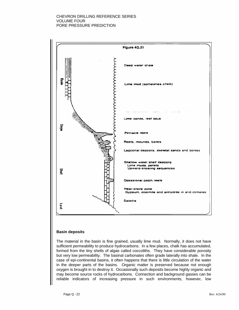
CHEVRON DRILLING REFERENCE SERIESVOLUME FOURPORE PRESSURE PREDICTION
Page Q - 22 Rev. 4/24/90
Basin deposits
The material in the basin is fine grained, usually lime mud. Normally, it does not havesufficient permeability to produce hydrocarbons. In a few places, chalk has accumulated,formed from the tiny shells of algae called coccoliths. They have considerable porositybut very low permeability. The basinal carbonates often grade laterally into shale. In thecase of epi-continental basins, it often happens that there is little circulation of the waterin the deeper parts of the basins. Organic matter is preserved because not enoughoxygen is brought in to destroy it. Occasionally such deposits become highly organic andmay become source rocks of hydrocarbons. Connection and background gasses can bereliable indicators of increasing pressure in such environments, however, low
CHEVRON DRILLING REFERENCE SERIESVOLUME FOUR
PORE PRESSURE PREDICTION
Page Q - 23 Rev. 4/24/90
permeability is generally likely. Such formations typically provide low volumes and ratesof flow when drilled under-balanced.
Limestones experience a lithification process. When originally deposited, lime mudshave a porosity of 50 percent or more, but when they are consolidated into limestonetheir porosity is generally less than two percent. Shales lose porosity by a compactionprocess that involves flattening. However, limestones are formed from lime mud byrecrystallization, and the pores are filled by precipitation of calcite, apparently brought infrom elsewhere, because no compaction has occurred. Oolites and fossils are notsquashed and flattened. Where did the calcite come from that filled the pores?
Limestones are often partially or completely changed to dolomite. Dolomite has thecomposition CaMgCO3 and it is crystallographically similar to calcite. However, it hasgreater density, less solubility in water, less ductility, and more brittleness.
Dolomites are always found in the shelf environment, near in the deep basin. They arecommonly associated with evaporites (salt and especially gypsum and anhydrite) andwith stromatolites, which are layers of algael mats.
There is no doubt that dolomites generally are more porous and permeable thanlimestones.
An illustration of fracture porosity and tension type fractures appears in Figure 4Q.22.When sandstones are sharply folded, the beds slide over each other; but whencarbonates are folded or faulted, they develop fractures. If the stress environment iscompressional, as it often is along faults and sharp folds, the fractures may be tightlyclosed. In this case the porosity due to the fractures will be negligible, and even thepermeability will not be very great. Much more prolific are fractures resulting fromtension. Over an anticlinal told, tensional fractures are perpendicular to the bedding andeither parallel to the axis of the fold or, more commonly, at right angles to it. If fracturesare anticipated in a tension environment, lost circulation is possible.
Fractures usually have a volume of less than 1 percent of the rock, while the matrix mayhave a porosity of 5 to 10 percent. Consequently, fractures contribute much more to thepermeability of a reservoir than to its porosity.
An illustration of chalk appears in Figure 4Q.23. Chalk is formed from microscopic algaecalled coccoliths. Their tiny ring-shaped shells, 1-20 um in diameter, were made ofcalcite. These settled to the bottom, forming a thickness of chalk. Chalk is anexceedingly pure carbonate rock, soft, white and porous, that contains very littleterrigenous material. Locally, the chalk may contain small amounts of shell debris.Nodules of chert are common. When first deposited on the sea bottom, the porosity ofthe shells is 70%. With increasing depth of burial, porosity is lost rapidly. Some of theloss is due to mechanical compaction and some to chemical cementation. At a depth of

CHEVRON DRILLING REFERENCE SERIESVOLUME FOURPORE PRESSURE PREDICTION
Page Q - 24 Rev. 4/24/90
burial of 1,000 m, the porosity of most chalk is reduced to about 35%, at 000 m to 15%,and at 3 km practically to zero. The permeability of chalk is typically very low becausethe particle size is so fine. It decreases from about 10 md at 40% porosity to 0.1 md at10%. Chalk is also a good seismic reflector.
Quite simply put, the origin of reservoir pressures appears in Figure 4Q.24. In the cross-section, the aquifer outcrops at A. There are three oil fields in the same aquifer: B, C,
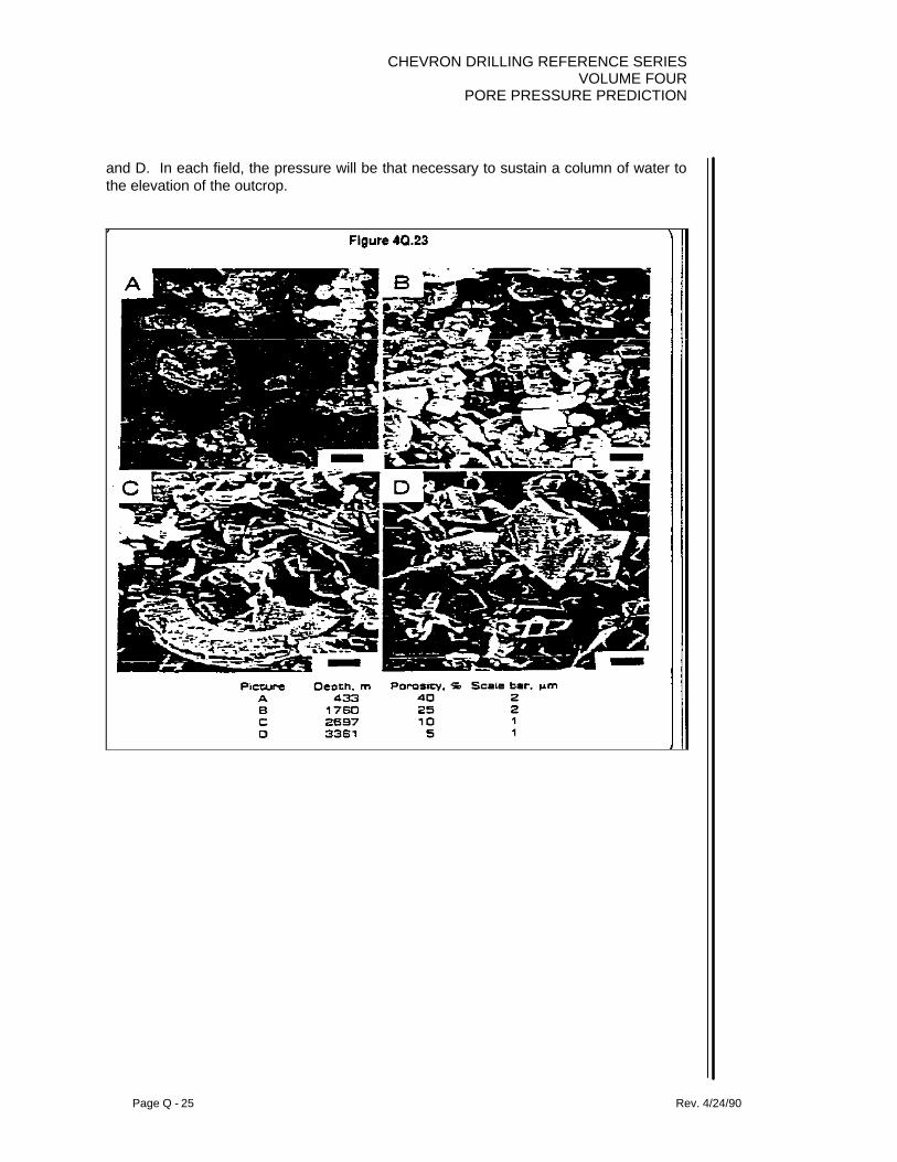
CHEVRON DRILLING REFERENCE SERIESVOLUME FOUR
PORE PRESSURE PREDICTION
Page Q - 25 Rev. 4/24/90
and D. In each field, the pressure will be that necessary to sustain a column of water tothe elevation of the outcrop.

CHEVRON DRILLING REFERENCE SERIESVOLUME FOURPORE PRESSURE PREDICTION
Page Q - 26 Rev. 4/24/90
2. ORIGIN OF LOW PRESSURES
The low-pressure reservoirs are in well-consolidated sediments which have been upliftedin the recent geologic past, and which are now undergoing erosion.
Figure 4Q.24b
OTHER FACTORS CAUSING HIGH PRESSURE
As sedimentation continues, depth of burial increases and temperatures increase, Thiscauses an increase in the volume of the pore water. If the system is effectively confined,pore pressures will increase.
At temperatures of about 100°C or depths between 8,000 and 10,000 feet (2,500 and3,000), smectite converts to illite. This involves a loss of interlattice water. If there is anincrease in specific volume of the water as it comes out of the smectite or if the smectite

CHEVRON DRILLING REFERENCE SERIESVOLUME FOUR
PORE PRESSURE PREDICTION
Page Q - 27 Rev. 4/24/90
Figure 4Q.24a
ORIGIN OF LOW PRESSURES
The low-pressure reservoirs are in well-consolidated sediments which have beenuplifted in the recent geologic past, and which are now undergoing erosion.
A sandstone reservoir contracts elastically about 7 x 10⁻⁶ pore volumes per porevolume per psi (5 x 10⁻⁵ pv per kPa) as the internal pressure of the fluids inremoved. This is an elastic compression and should not be confused withcompaction, which is irreversible. The removal of overburden will cause an elasticdilation of the sandstone at about the same rate. Shales appear to contract anddilate even more than sandstones. The modulus of compressibility of water isabout 3 x 10⁻⁶ volumes per volume per psi (4 x 10⁻⁷ vol/vol/kPa). Therefore, asoverburden is removed, the pore volume dilates but the interstitial water expandsonly about half as much as necessary to fill the new pore volume thus created.Consequently, its pressure will drop.
For the reservoir to remain at subnormal pressure, we must assume that theoverlying shales are completely impermeable. Otherwise, the ground water wouldfilter down and pressure up the aquifer.
Figure 4Q.24c
SHALE GAS ON MUD LOGGER
If the pore pressure is higher than the mud pressure the shales tend to spall and caveinto the hole. If the pore water in the shales is saturated with methane, as is often thecase, it comes out of solution on the way up the hole and makes a strong indication inthe gas-measuring device in the mud logger.
Figure 4Q.24d
Shale and Carbonate Gas (background & connection gases)
Current information dealing with the organic origin of petroleum indicates thathydrocarbons are products of altered organic material derived from microscopic plant andanimal life.
As deposition of the organic material takes place in the marine environment, it is buriedand protected by the clay and silt that accompanies it. This prevents decomposition ofthe organic material and allows it to accumulate.
Conversion of the organic material is apparently assisted by pressure caused by burial,temperature resulting from depth and bacterial action in a closed non-oxidizing chemicalsystem. Accumulation of organic and classic material on the sea bottom is accompaniedby bacterial action. if there is abundant oxygen, aerobic bacteria act upon the organicmatter and destroy it. However, the aerobic destruction of organic matter is greatlyreduced or eliminated if enough low permeability sediment is deposited to stop thecirculation of oxygen-bearing water. As aerobic bacterial action ceases with thedecrease in available dissolved oxygen, anaerobic bacterial action involving oxygen fromdissolved sulfates begins and a reducing environment develops.
Shale and some carbonates contain organic material that bears hydrocarbons. Shaleand carbonate rocks of this type are not reservoir-type rocks and could be consideredultimately to be source beds.
Diagenesis of source-type rocks eliminates some of these organic materials but allowsretention of residual amounts that are found in some quantities in most non-reservoirrocks.
Therefore, if aerobic bacteria can act, there will be no shale or carbonate gas. If theycannot act, there will be shale or carbonate gas. (Background or connection gas)geologic past, and which are now undergoing erosion.
CHEVRON DRILLING REFERENCE SERIESVOLUME FOURPORE PRESSURE PREDICTION
Page Q - 28 Rev. 4/24/90
A sandstone reservoir contracts elastically about 7 x 10⁻⁶ pore volumes per pore volumeper psi (5 x 10⁻⁵ pv per kPa) as the internal pressure of the fluids is removed. This is anelastic compression and should not be confused with compaction, which is irreversible.The removal of overburden will cause an elastic dilation of the sandstone at about thesame rate. Shales appear to contract and dilate even more than sandstones. Themodulus of compressibility of water is about 3 x 10⁻⁶ volumes per volume per psi (4 x 10⁻⁷
vol/vol/kPa). Therefore, as overburden is removed, the pore volume dilates but theinterstitial water expands only about half as much as necessary to fill the new porevolume thus created. Consequently, its pressure will drop.
For the reservoir to remain at subnormal pressure, we must assume that the overlyingshales are completely impermeable. Otherwise, the ground water would filter down andpressure up the aquifer.
3. OTHER FACTORS CAUSING HIGH PRESSURE
As sedimentation continues, depth of burial increases and temperatures increase. Thiscauses an increase in the volume of the pore water. If the system is effectively confined,pore pressures will increase.
At temperatures of about 100°C or depths between 8,000 and 10,000 ft. (2,500 and3,000), smectite converts to illite. This involves a loss of interlattice water. If there is anincrease in specific volume of the water as it comes out of the smectite, or if the smectiteloses volume, it could cause an increase in pore pressure.
4. SHALE GAS ON MUD LOGGER
If the pore pressure is higher than the mud pressure the shales tend to spall and caveinto the hole. It the pore water in the shales is saturated with methane, as is often thecase, it comes out of solution on the way up the hole and makes a strong indication inthe gas-measuring device in the mud logger.
Shale and Carbonate Gas (background and connection gases)
Current information dealing with the organic origin of petroleum indicates thathydrocarbons are products of altered organic material derived from microscopic plant andanimal life.
CHEVRON DRILLING REFERENCE SERIESVOLUME FOUR
PORE PRESSURE PREDICTION
Page Q - 29 Rev. 4/24/90
As deposition of the organic material takes place in the marine environment, it is buriedand protected by the clay and silt that accompanies it. This prevents decomposition ofthe organic material and allows it to accumulate.
Conversion of the organic material takes place in the marine environment, it is buried andprotected by the clay and silt that accompanies it. This prevents decomposition of theorganic material and allows it to accumulate.
Conversion of the organic material is apparently assisted by pressure caused by burial,temperature resulting from depth and bacterial action in a closed non-oxidizing chemicalsystem. Accumulation of organic and clastic material on the sea bottom is accompaniedby bacterial action. If there is abundant oxygen, aerobic bacteria act upon the organicmatter and destroy it. However, the aerobic destruction of organic matter is greatlyreduced or eliminated if enough low permeability sediment is deposited to stop thecirculation of oxygen-bearing water. As aerobic bacterial action cease with the decreasein available dissolved oxygen, anaerobic bacterial action involving oxygen from dissolvedsulfates begins and a reducing environment develops.
Shale and some carbonates contain organic material that bears hydrocarbons. Shaleand carbonate rocks of this type are not reservoir-type rocks and could be consideredultimately to be source beds.
Diagenesis of source-type rocks eliminates some of these organic materials but allowsretention of residual amounts that are found in some quantities in most non-reservoirrocks.
Therefore, if aerobic bacteria can act, there will be no shale or carbonate gas. If theycannot act, there will be shale or carbonate gas (background or connection gas).
The vertical stresses existing in sediments appear in Figure 4Q.25. When the pressurein the pore water approaches the weight of the over-burden, the overlying strata arepractically floating.
The weight of the overburden (S) is sustained by the stress in the skeleton of the solidgrains % and the pore pressure (p) in the interstitial fluids.
S = % + p
As p increases, % decreases and may become very small. That is, the solid skeleton issupporting very little weight, and the overlying strata are floating. They can slide underweak lateral forces, such as gravity sliding if the area is tectonically tilted.

CHEVRON DRILLING REFERENCE SERIESVOLUME FOURPORE PRESSURE PREDICTION
Page Q - 30 Rev. 4/24/90
Most, it not all, low-angle thrust faults probably take place in a zone of abnormally highpressure. A seismic illustration of growth type faulting with featureless shale zonesappears in Figure 4Q.26. Seismic cross-sections clearly show the faults and dips of thestratified beds. They also show where the shale has become chaotic below the faultplanes. Some of these featureless shale zones may be caused by diapirism deep belowthe surface, while others may represent the toe zone of the slump block where the faultemerges at the surface, part way down the continental slope,
Shale in the chaotic zone is under-compacted and contains fluids at pressures almostequal to the weight of the overburden. An under-compacted bed is less dense than anormally compacted bid. It, therefore, is unstable and has a tendency to be forcedupward.
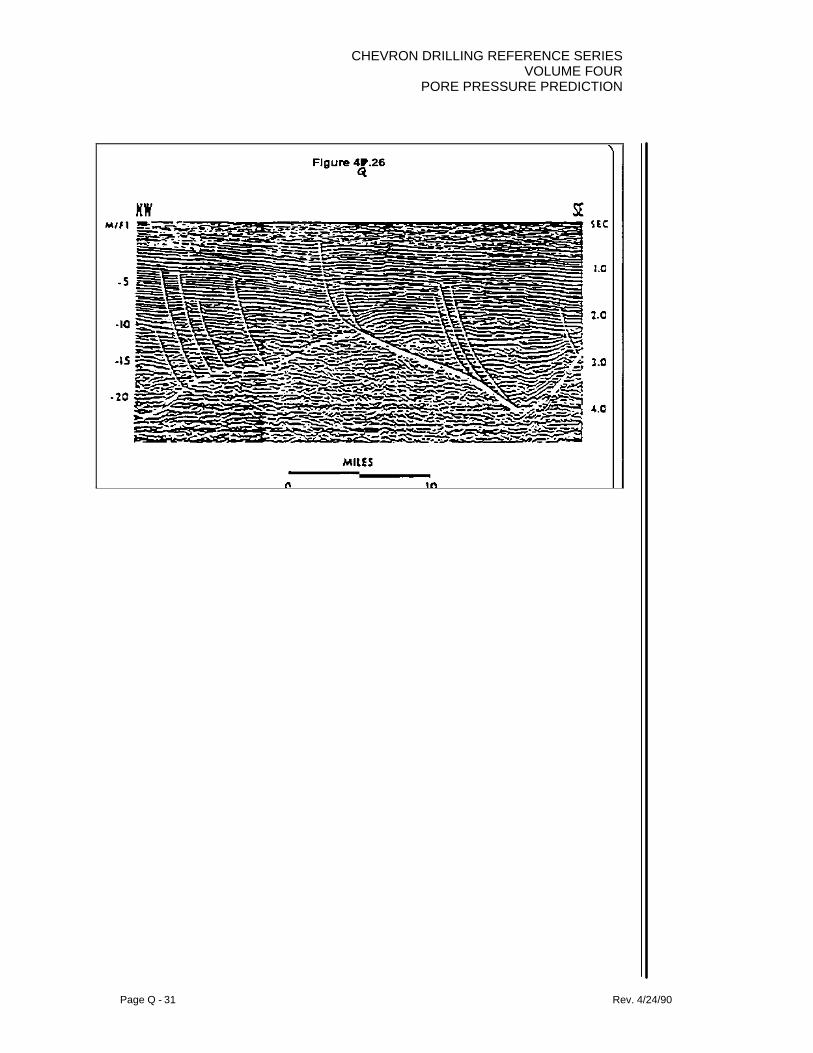
CHEVRON DRILLING REFERENCE SERIESVOLUME FOUR
PORE PRESSURE PREDICTION
Page Q - 31 Rev. 4/24/90

CHEVRON DRILLING REFERENCE SERIESVOLUME FOURPORE PRESSURE PREDICTION
Page Q - 32 Rev. 4/24/90

CHEVRON DRILLING REFERENCE SERIESVOLUME FOUR
PORE PRESSURE PREDICTION
Page R - 1 Rev. 4/24/90
SECTION R: THE BOREHOLE BALLOONINGPHENOMENA
1. BACKGROUND
We are currently studying the problem of borehole stability from several aspects at theDTC; whether it is due to abnormally pressured shale, borehole inclination, claychemistry, etc., as well as pursuing any industry data or research on the subject. Theproblem appears to be a very complex one with many contributing factors.
Chevron, through the DTC, has participated in studies evaluating the effects of variousmud additives on bore hole stability which have yielded many significant results. Inaddition, Chevron participates in associated joint industry DEA projects. We havedeveloped numerous techniques within Chevron for the determination of formation porepressures and, in comparison to all others, find them to be the most accurate available inthe industry today.
We have investigated several Chevron wells where “borehole ballooning" has takenplace. When all the necessary data has been available for a complete analysis, we findour problem primarily relates to a combination of a lack of detailed formation porepressure analysis, inadequate rock composition analysis, and excessive surge pressuresexerted on the borehole while tripping pipe.
The ballooning effects are generally seen in the deeper sections of our wellbores belowan intermediate string of casing. Once intermediate casing is set, we have a longpiston/cylinder relationship in place. Intermediate pipe is set in some mud weight and aformation integrity test below the casing shoe is made. Generally the formation integrityat this intermediate shoe is much higher, in mud weight equivalent, than the mud weightcasing was set in.
As drilling progresses to deeper depths and higher pressures are encountered, the mudweight is increased to balance this higher pressure. As our mud weights increase, theyapproach the magnitude of the intermediate shoe integrity. During a trip to change bits itbecomes very easy to initiate a fracture in the formations just below the casing shoe dueto the long piston/cylinder relationship we have between the drill string and the casing.The combination of mud weight in the hole and the surge pressure created while trippingin the hole can exceed the formation integrity, thus initiating a fracture in the formation.
Once a fracture has been initiated, extension of the fracture can be made at a lowerpressure, or at a lower mud weight equivalent. If the mud weight in the hole at the timeof fracture initiation is below the extension pressure, then the hole stays full at the time offracture initiation. As drilling progresses to even deeper depths and higher pressures are

CHEVRON DRILLING REFERENCE SERIESVOLUME FOURPORE PRESSURE PREDICTION
Page R - 2 Rev. 4/24/90
encountered, the mud weight is raised further. We then get to a point where acombination of the mud weight in the hole and the friction pressures due to circulationexceed the fracture extension pressure and consequently we begin to lose mud whiledrilling as mud begins to extend the fractures. When we stop circulation, the mud weightalone, without the help of friction pressures, no longer exceeds fracture extensionpressure. The forces of the overburden now act in trying to force the fractures closed,resulting in squeezing the mud back into the wellbore, or appearing to flow.
In many areas of the country we also encounter, as our drilling proceeds below a casingshoe, naturally fractured formations. With these naturally fractured formations we caninduce the same phenomena as above.
When utilizing oil base drilling fluids, a close relationship exists between the requiredwater phase salinity of the mud, and the salinity of the formations drilled and formationpore pressure. Exceeding the required water-phase salinity of the mud results inchemically altering the formation rocks by drying due to osmotic forces. This chemicalalteration can result in subsequently weakening the rock and lead to a reduction infracture initiation pressure. A similar "ballooning" relationship can then be experiencedas previously described. This problem with oil based drilling fluids is further complicatedby the compressibility of the fluid yielding higher mud weight equivalents down hole thanseen at the surface.
In all instances of a “ballooning experience" investigated we have found the above to betrue. Never have we been able to find a case of an expanding and contracting borehole.In all wells where flow was experienced without any mud losses to fractures, porepressure analyses have determined an under-balanced condition to exist. In many lowpermeability, hard formations, we are able to drill under balanced with low rates andvolumes of flow into the wellbore. In addition, many of our troublesome shales, we'refinding, are abnormally pressured though the surrounding permeable formations arenormally pressured. Consequently, the drilling of such shales, unknowingly underbalanced, leads to instability problems.
It has been proposed to Chevron, by Mr. Gill, that borehole ballooning of the expandingand contracting borehole theory, is the cause of our need of high mud weights in theMobile wells. It has been suggested that our Mobile wells are in actuality, normallypressured. However, our in house techniques of analysis suggest the contrary. In thedrilling of the Mobile 861 No. 1, the Norphlet was encountered with a 16.7 ppg mud whichresulted in a kick and an underground blowout. Chevron's analysis of the pressures seenindicated the Norphlet to be a 17.2 ppg pore pressure. In the Mobile 862 No 2, wetherefore, drilled the Norphlet with a 17.4 ppg mud. No problems were encountered andthe well was successfully drilled. By Mr. Gill's theory, we should have encounteredproblems with a ballooning borehole but did not. Whenever we drill wells in anabnormally pressured environment, as we weight up the drilling fluid to handle the higherpressures seen, we expose the lower pressured formations up the hole to highdifferential pressures. By Mr. Gill's theory this would always create an impossiblesituation of flow from these shallower formations, making it impossible for us to drill inabnormally pressured environments. However, this problem does not occur.
CHEVRON DRILLING REFERENCE SERIESVOLUME FOUR
PORE PRESSURE PREDICTION
Page R - 3 Rev. 4/24/90
We at Chevron have visited with Mr. Gill on several occasions to discuss his theories.He claims faster penetration rates to be the result of ballooning. However, on numerousabnormally pressured wells we observe increases in penetration rates associated withincreasing pore pressure with no associated ballooning. He states that connectiongasses are never seen above 120 units. Many times we experience much higher valuesthan this in our operations in abnormally pressured environments with valid bottom holepressures recorded to verify the presence of abnormal pressure. Mr. Gill claims thatthere are no abnormally pressured reservoirs, but he has no explanation for thenumerous production histories we have in such abnormally pressured environments. Heinsists the Mobile wells we've drilled are normally pressured but is unable to explain theabnormally pressured underground flow we experienced for months in the 861 No. 1 well.
Mr. Gill's paper was reviewed twice by two groups of Co-Technical editorials plus theiradvisors, the SPE Editorial Review Committee. On both occasions his paper wasdeclined for publication because of lack of technical merit and composition.
Mr. Gill has approached some of our drilling superintendents in the past with his conceptsof the "ballooning" borehole which resulted in drilling abnormally pressured wells underbalanced, kicks, stuck pipe and lost hole. We can attribute several lost holes in ouroperations due to employment of his theories. We see him and his theories as verydangerous to the industry.
The solution to many of our instability problems can be solved through an increasedunderstanding of the environment we are about to drill. This can be developed through adetailed pore pressure analysis, rock composition analysis via logs, mud logs, cores andpaleo data, and a better understanding of the structural relationship between wellssurface to total depth. This would require a change in philosophy, as a company, fromone of reactionary, and rushing our drilling prospects from every planning aspect, to thatof a detailed planning approach and project team analysis.
2. DISCUSSION
Numerous wells, where the so called "borehole ballooning" has taken place, wereevaluated in an effort to determine the mechanism by which we experience either one oftwo phenomena. One being the gradual loss of drilling mud to the wellbore while drilling,followed by a flow back of the mud whenever the pumps were stopped. The secondbeing the low volume, low rate influxes of formation water into the wellbore both whiledrilling or with the pumps off, without any associated mud losses. Generally these lowrate influxes have been on the order of 1/4 to 1 barrel of influx per hour. When all thenecessary data has been available for a complete analysis, we find our problem primarilyrelates to a combination of a lack of detailed formation pore pressure analysis,inadequate rock composition analysis, and excessive surge pressures exerted on theborehole while tripping pipe.

CHEVRON DRILLING REFERENCE SERIESVOLUME FOURPORE PRESSURE PREDICTION
Page R - 4 Rev. 4/24/90
The ballooning effects which are characterized by the gradual mud loss while drilling, witha flow back with the pump off, are generally seen in the deeper sections of our wellboresbelow an intermediate string of casing. Once intermediate casing is set, we have a longpiston/cylinder relationship in place, with the casing acting as a cylinder and the drillstring acting as a piston. Intermediate pipe is set in some mud weight and a formationintegrity test below the casing shoe is made. Generally the formation integrity at thisintermediate shoe is much higher, in mud weight equivalent, than the mud weight casingwas set in.
As drilling progresses to deeper depths and higher pressures are encountered, the mudweight is increased to balance this higher pressure. As our mud weights increase, theyapproach the magnitude of the intermediate shoe integrity. During a trip to change bits itbecomes very easy to initiate a fracture in the formations just below the casing shoe dueto the long piston/cylinder relationship we have between the drill string and the casing, asillustrated in Figure 4R.1.
In Figure 4Q.1 we have set casing in a transition zone at a point where formation porepressure is 12 ppg mud weight equivalent. Upon drilling out of this casing shoe, aformation integrity test is taken yielding a 16.5 ppg equivalent. An illustration of therecorded data during the integrity test appears in the illustration as well. Note thedeviation from the straight line trend at a value of 16.5 ppg equivalent mud weightindicating leak off. Normally the test would have been concluded at the dashed linebefore formation break down had occurred. Beyond the dashed line we illustrategraphically as we continue with such a test and proceed to break down or fracture theformation. Note that we arrive at a fracture extension pressure of 15.5 ppg equivalentmud weight, somewhat below the leak off point. At this pressure, if constantly imposedon the wellbore, we could continue to extend formation fractures well beyond thewellbore as we pump fluid into the fracture.
The combination of mud weight in the hole and the surge pressure created while trippingin the hole can exceed the formation integrity, thus initiating a fracture in the formation.In this illustration the mud in the hole weighs 14.0 ppg due to currently drilling a formationof 13.5 ppg pore pressure. A pore pressure profile vs. depth for this example appears inthe illustration as well. The surge pressure exerted at the shoe due to flipping the drillstring is 3.0 ppg equivalent. The combination of mud weight and surge pressure yields a17.0 ppg equivalent mud weight at the casing shoe, thereby exceeding formation integrityand initiating fractures. If the mud weight in the hole at the time of fracture initiation isbelow the extension pressure, as it is in Figure 4R.1, then the hole stays full at the timeof fracture initiation.
Once a fracture has been initiated, extension of the fracture can be made at a lowerpressure, or at a lower mud weight equivalent. As drilling progresses to even deeperdepths and higher pressures are encountered, the mud weight is raised further, as inFigure 4R.2. Here we have arrived at a formation of approximately 15.0 ppg porepressure, necessitating a mud weighing 15.3 ppg. The friction pressures in the annulus

CHEVRON DRILLING REFERENCE SERIESVOLUME FOUR
PORE PRESSURE PREDICTION
Page R - 5 Rev. 4/24/90
due to mud circulation are equivalent to .4 ppg mud weight. The combination of mudweight and friction pressures equates to a 15.7 ppg equivalent thereby exceeding thefracture extension pressure of 15.5 ppg.
Figure 4R.1
INFORMATION REQUIRED FOR PORE PRESSUREANALYSIS AT PROPOSED LOCATION
1. Copies of structure maps. (small scale preferred)
2. One inch electric logs (with resistivity and conductivity on a linearscale) of at least three offset wells which penetrate as many of theexpected formations as possible, and on both sides of any majorfaulting. (not to be limited to three offsets)
3. On the same offsets as above, gamma ray and sonics displayed in thefollowing scales, one inch = 1000 feet and one inch = 100 feet (alsowith gamma ray and sonic values displayed on a linear scale).
NOTE: To display these curves in these reduced scales, a smoothingfunction will probably be required for the curves to be clear and readable.
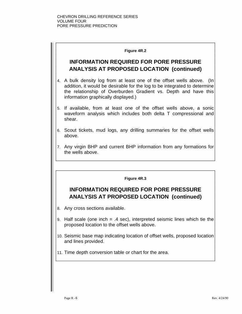
CHEVRON DRILLING REFERENCE SERIESVOLUME FOURPORE PRESSURE PREDICTION
Page R - 6 Rev. 4/24/90
Figure 4R.2
INFORMATION REQUIRED FOR PORE PRESSUREANALYSIS AT PROPOSED LOCATION (continued)
4. A bulk density log from at least one of the offset wells above. (Inaddition, it would be desirable for the log to be integrated to determinethe relationship of Overburden Gradient vs. Depth and have thisinformation graphically displayed.)
5. If available, from at least one of the offset wells above, a sonicwaveform analysis which includes both delta T compressional andshear.
6. Scout tickets, mud logs, any drilling summaries for the offset wellsabove.
7. Any virgin BHP and current BHP information from any formations forthe wells above.
Figure 4R.3
INFORMATION REQUIRED FOR PORE PRESSUREANALYSIS AT PROPOSED LOCATION (continued)
8. Any cross sections available.
9. Half scale (one inch = .4 sec), interpreted seismic lines which tie theproposed location to the offset wells above.
10. Seismic base map indicating location of offset wells, proposed locationand lines provided.
11. Time depth conversion table or chart for the area.
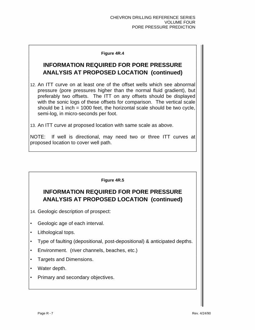
CHEVRON DRILLING REFERENCE SERIESVOLUME FOUR
PORE PRESSURE PREDICTION
Page R - 7 Rev. 4/24/90
Figure 4R.4
INFORMATION REQUIRED FOR PORE PRESSUREANALYSIS AT PROPOSED LOCATION (continued)
12. An ITT curve on at least one of the offset wells which see abnormalpressure (pore pressures higher than the normal fluid gradient), butpreferably two offsets. The ITT on any offsets should be displayedwith the sonic logs of these offsets for comparison. The vertical scaleshould be 1 inch = 1000 feet, the horizontal scale should be two cycle,semi-log, in micro-seconds per foot.
13. An ITT curve at proposed location with same scale as above. NOTE: If well is directional, may need two or three ITT curves atproposed location to cover well path.
Figure 4R.5
INFORMATION REQUIRED FOR PORE PRESSUREANALYSIS AT PROPOSED LOCATION (continued)
14. Geologic description of prospect:
• Geologic age of each interval.
• Lithological tops.
• Type of faulting (depositional, post-depositional) & anticipated depths.
• Environment. (river channels, beaches, etc.)
• Targets and Dimensions.
• Water depth.
• Primary and secondary objectives.

CHEVRON DRILLING REFERENCE SERIESVOLUME FOURPORE PRESSURE PREDICTION
Page R - 8 Rev. 4/24/90
We then get to a point where a combination of the mud weight in the hole and the frictionpressures due to circulation exceed the fracture extension pressure. Consequently, at amud weight below the formation integrity test, we 'mysteriously' begin to lose mud whiledrilling as mud begins to extend the fractures.
When we stop circulation, the mud weight alone, without the help of friction pressures, nolonger exceeds fracture extension pressure as in Figure 4R.3. The forces of theoverburden now act in trying to force the fractures closed, resulting in squeezing the mudback into the wellbore, or appearing to flow. We now have developed a ballooningappearance with loss of mud to the wellbore while drilling, and flow back with the pumpsoff.
In many areas of the country we also encounter, as our drilling proceeds below a casingshoe, naturally fractured formations. With these naturally fractured formations we caninduce the same phenomena as above.
A similar occurrence exists when using oil based drilling fluids, however, an additionalfracture initiation mechanism also exists. When utilizing oil base drilling fluids, a closerelationship exists between the required water phase salinity of the mud, and the salinityof the formations drilled and formation pore pressure. The water phase salinitiesrequired for stability are illustrated in Figure 4R.4.
Exceeding the required water phase salinity of the mud results in chemically altering theformation rocks by drying due to osmotic forces. This chemical alteration can result inweakening the rock and can lead to a reduction in fracture initiation pressure. A similar“ballooning" relationship can then be experienced as previously described. This problemwith oil based drilling fluids is further complicated by the compressibility of the fluidyielding higher mud weight equivalents downhole than seen at the surface.
In all instances of a “ballooning experience” investigated we have found the above to betrue. Never have we been able to find a case of an expanding and contracting borehole.If this theory indeed had significant applications, drilling in abnormally pressuredenvironments would be almost impossible. As illustrated by Figure 4R.5, as we increaseour mud weight while drilling in response to increasing pore pressures, we expose thelower pressured formations still exposed up the hole to high differentials. By theexpanding/contracting ballooning borehole theory, this should cause a ballooningresponse and flow. However, this has never been the case.
In all wells where flow was experienced without any mud losses to fractures, porepressure analyses have determined an under balanced condition to exist. In many lowpermeability hard formations, we are able to drill under balanced with low rates andvolumes of flow into the wellbore. This is illustrated in the following two examples.

CHEVRON DRILLING REFERENCE SERIESVOLUME FOUR
PORE PRESSURE PREDICTION
Page R - 9 Rev. 4/24/90
In Figure 4R.6 we have a graphical display of pore pressure and mud weight used vs.depth for the Destin Dome 422 No. 1 well. Note from approximately 15,000 to 22,000feet the mud weight used falls below pore pressure determinations. Throughout thisinterval, while drilling the well, influxes of 1/2 to 3/4 barrels per hour of formation waterwere encountered. As expected, this occurred due to an under balanced condition whilepenetrating hard, low permeability formations.
Figure 4R.7 is a graphical display of pore pressure and mud weight used vs. depth forthe Mobile 862 No. 1 well. Note at a depth of 19,741, while tripping pipe out of the hole,an influx of approximately 3/4 barrels per hour was encountered. This was due toencountering a low permeability salt water formation under balanced at this point. Afterthe trip the mud weight was gradually raised to exceed the pore pressures and with a15.8 ppg mud in the hole, no influx of fluid was experienced on subsequent trips.
CHEVRON DRILLING REFERENCE SERIESVOLUME FOURPORE PRESSURE PREDICTION
Page R - 10 Rev. 4/24/90
In addition, many of our troublesome shales, we're finding, are abnormally pressuredalthough the surrounding permeable formations are normally pressured. Consequently,the drilling of such shales, unknowingly under balanced, leads to instability problems. InFigure 4R.8 we have an illustration of pore pressure and mud weight used vs. depth for awell drilled offshore California from platform Hermosa. A detailed pore pressure analysisindicates the traditionally troublesome shale interval on this platform between 5,000 and6,000 feet to be abnormally pressured in the vicinity of 11.2 ppg pore pressure.Traditionally this interval was drilled with 10.0 ppg mud or less with a great deal of shaleheavings and in some cases stuck pipe. A rate of penetration plot for this intervalappears in Figure 4R.9. The rate of penetration is on a logarithmic scale. Note thatpenetration rates increase significantly and regress through this interval confirming thepresence of an abnormally pressured interval. Due to this analysis, a more recent wellwas drilled with a higher mud weight closer to balancing the shale pore pressure. Whenthis was done, the shale heaving problem disappeared.
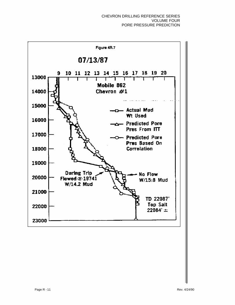
CHEVRON DRILLING REFERENCE SERIESVOLUME FOUR
PORE PRESSURE PREDICTION
Page R - 11 Rev. 4/24/90

CHEVRON DRILLING REFERENCE SERIESVOLUME FOURPORE PRESSURE PREDICTION
Page R - 12 Rev. 4/24/90
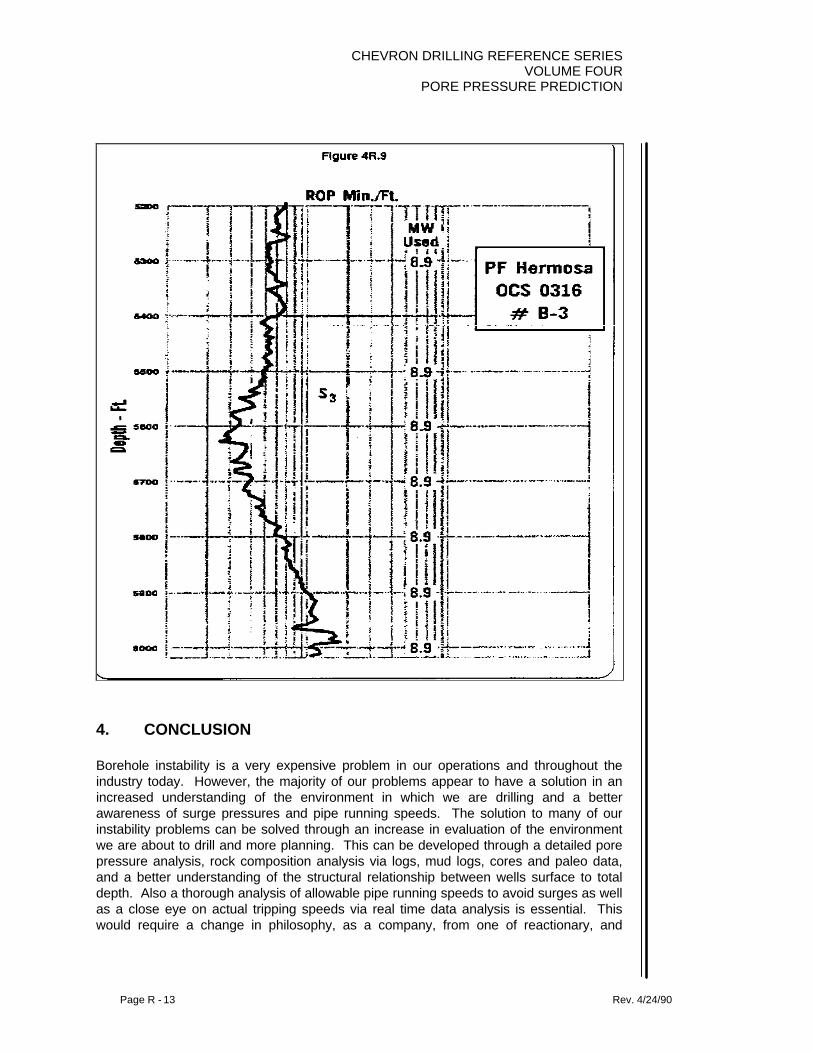
CHEVRON DRILLING REFERENCE SERIESVOLUME FOUR
PORE PRESSURE PREDICTION
Page R - 13 Rev. 4/24/90
4. CONCLUSION
Borehole instability is a very expensive problem in our operations and throughout theindustry today. However, the majority of our problems appear to have a solution in anincreased understanding of the environment in which we are drilling and a betterawareness of surge pressures and pipe running speeds. The solution to many of ourinstability problems can be solved through an increase in evaluation of the environmentwe are about to drill and more planning. This can be developed through a detailed porepressure analysis, rock composition analysis via logs, mud logs, cores and paleo data,and a better understanding of the structural relationship between wells surface to totaldepth. Also a thorough analysis of allowable pipe running speeds to avoid surges as wellas a close eye on actual tripping speeds via real time data analysis is essential. Thiswould require a change in philosophy, as a company, from one of reactionary, and
CHEVRON DRILLING REFERENCE SERIESVOLUME FOURPORE PRESSURE PREDICTION
Page R - 14 Rev. 4/24/90
rushing our drilling prospects from every planning aspect, to that of a detailed planningapproach and project team analysis.
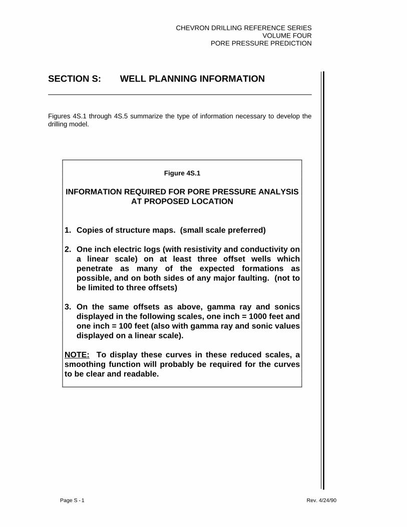
CHEVRON DRILLING REFERENCE SERIESVOLUME FOUR
PORE PRESSURE PREDICTION
Page S - 1 Rev. 4/24/90
SECTION S: WELL PLANNING INFORMATION
Figures 4S.1 through 4S.5 summarize the type of information necessary to develop thedrilling model.
Figure 4S.1
INFORMATION REQUIRED FOR PORE PRESSURE ANALYSISAT PROPOSED LOCATION
1. Copies of structure maps. (small scale preferred) 2. One inch electric logs (with resistivity and conductivity on
a linear scale) on at least three offset wells whichpenetrate as many of the expected formations aspossible, and on both sides of any major faulting. (not tobe limited to three offsets)
3. On the same offsets as above, gamma ray and sonics
displayed in the following scales, one inch = 1000 feet andone inch = 100 feet (also with gamma ray and sonic valuesdisplayed on a linear scale).
NOTE: To display these curves in these reduced scales, asmoothing function will probably be required for the curvesto be clear and readable.
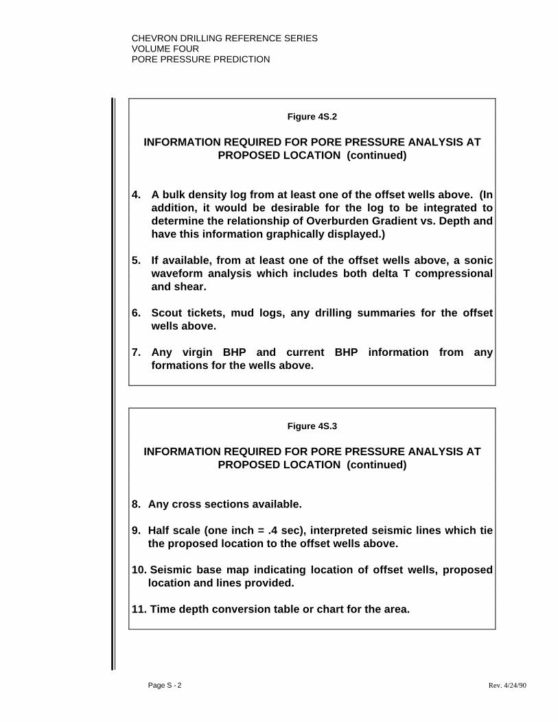
CHEVRON DRILLING REFERENCE SERIESVOLUME FOURPORE PRESSURE PREDICTION
Page S - 2 Rev. 4/24/90
Figure 4S.2
INFORMATION REQUIRED FOR PORE PRESSURE ANALYSIS ATPROPOSED LOCATION (continued)
4. A bulk density log from at least one of the offset wells above. (Inaddition, it would be desirable for the log to be integrated todetermine the relationship of Overburden Gradient vs. Depth andhave this information graphically displayed.)
5. If available, from at least one of the offset wells above, a sonicwaveform analysis which includes both delta T compressionaland shear.
6. Scout tickets, mud logs, any drilling summaries for the offsetwells above.
7. Any virgin BHP and current BHP information from anyformations for the wells above.
Figure 4S.3
INFORMATION REQUIRED FOR PORE PRESSURE ANALYSIS ATPROPOSED LOCATION (continued)
8. Any cross sections available.
9. Half scale (one inch = .4 sec), interpreted seismic lines which tiethe proposed location to the offset wells above.
10. Seismic base map indicating location of offset wells, proposedlocation and lines provided.
11. Time depth conversion table or chart for the area.

CHEVRON DRILLING REFERENCE SERIESVOLUME FOUR
PORE PRESSURE PREDICTION
Page S - 3 Rev. 4/24/90
Figure 4S.4
INFORMATION REQUIRED FOR PORE PRESSURE ANALYSIS ATPROPOSED LOCATION (continued)
12. An ITT curve on at least one of the offset wells which seeabnormal pressure (pore pressures higher than the normal fluidgradient), but preferably two offsets. The ITT on any offsetsshould be displayed with the sonic logs of these offsets forcomparison. The vertical scale should be one inch = 1000 feet,the horizontal scale should be two cycle, semilog, in micro-seconds per foot.
13. An ITT curve at the proposed location with same scale as above.NOTE: If well is directional, may need two or three ITT curves atproposed location to cover well path.
Figure 4S.5
INFORMATION REQUIRED FOR PORE PRESSURE ANALYSIS ATPROPOSED LOCATION (continued)
14. Geologic description of prospect: a. Geologic age of each interval.b. Lithological tops.c. Type of faulting (depositional, post-depositional) and anticipated depths.d. Environment (river channels, beaches, etc.)e. Targets and Dimensions.f. Water depthg. Primary and secondary objectives.
15. Paleo data.
16. Shallow hazards report.

CHEVRON DRILLING REFERENCE SERIESVOLUME FOURPORE PRESSURE PREDICTION
Page S - 4 Rev. 4/24/90

CHEVRON DRILLING REFERENCE SERIESVOLUME FOUR
PORE PRESSURE PREDICTION
Page T - 1 Rev. 4/24/90
SECTION T: ROP PLOTS
An additional pore pressure indication tool that can be used quite successfully is apenetration rate plot or ROP for simplicity. Any time a mud logger is used on a well, theyplot some sort of ROP plot for correlation purposes. However, varying the scale can beextremely beneficial or helpful in both correlating and in the determination of higher porepressures on a well. The illustration in Figure 4T.1 is a type of paper we use to plot aparticular ROP plot or a scale used. It is triple cycle semi-logarithmic paper and we plotvalues of penetration rates from geolograph charts. Every 5 feet, we plot the averagepenetration rate in minutes per foot along the semi-logarithmic scale, and we plot downthe depth scale or the vertical scale of 1 inch = 100 feet.
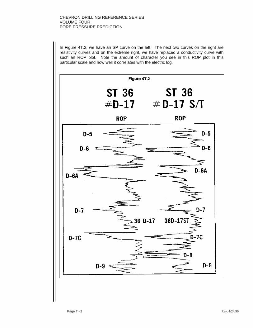
CHEVRON DRILLING REFERENCE SERIESVOLUME FOURPORE PRESSURE PREDICTION
Page T - 2 Rev. 4/24/90
In Figure 4T.2, we have an SP curve on the left. The next two curves on the right areresistivity curves and on the extreme right, we have replaced a conductivity curve withsuch an ROP plot. Note the amount of character you see in this ROP plot in thisparticular scale and how well it correlates with the electric log.

CHEVRON DRILLING REFERENCE SERIESVOLUME FOUR
PORE PRESSURE PREDICTION
Page T - 3 Rev. 4/24/90
It is also useful to correlate ROP’s with offset ROP’s such as in Figure 4T.3, where wehave the ROP on a side track hole versus an original hole. Here we can also see thesignificant changes in lithology which occur.
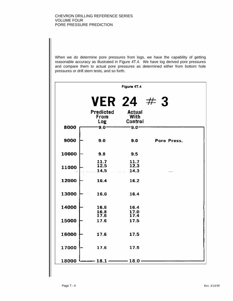
CHEVRON DRILLING REFERENCE SERIESVOLUME FOURPORE PRESSURE PREDICTION
Page T - 4 Rev. 4/24/90
When we do determine pore pressures from logs, we have the capability of gettingreasonable accuracy as illustrated in Figure 4T.4. We have log derived pore pressuresand compare them to actual pore pressures as determined either from bottom holepressures or drill stem tests, and so forth.

CHEVRON DRILLING REFERENCE SERIESVOLUME FOURPORE PRESSURE PREDICTION
Page T - 6 Rev. 4/24/90
You can see that we can get fairly accurate. Graphically illustrating this in Figure 4T.5,you can see that log drive pore pressures and actual pore pressures can be fairly close.

CHEVRON DRILLING REFERENCE SERIESVOLUME FOUR
PORE PRESSURE PREDICTION
Page T - 7 Rev. 4/24/90
In Figure 4T.6, we have the results of studies concerning differential sticking. It isimportant for us to know when our formations of given pore pressure are approachedrequiring higher mud weights, since we need to be aware of pore pressures up the holeand what that is doing differentially.

CHEVRON DRILLING REFERENCE SERIESVOLUME FOURPORE PRESSURE PREDICTION
Page T - 8 Rev. 4/24/90
In Figure 4T.7, we have an ROP plot. Notice at the bottom section, we have a gradualincrease in penetration rate drifting to the left. If we hold all things constant such as bitweight, mud weight, rotary speed, etc., then there are only two things which can affectpenetration rate. One is a lithology change and the other is pore pressure. Lithologicalchanges from shales to sands are indicated by very rapid increases in penetration rate.We pick up the sand tops in this fashion, however, the gradual increase in penetrationrate noted at the bottom of the hole, since this is a shale section, can only be due to anincrease in pore pressure. This gradual increase in penetration rate is not obvious whenplotted on other scales. If we plot on a linear scale, it is masked completely. Thisparticular scale exaggerates and picks it up quite well.

CHEVRON DRILLING REFERENCE SERIESVOLUME FOUR
PORE PRESSURE PREDICTION
Page T - 9 Rev. 4/24/90
In Figure 4T.8, we have replaced a conductivity curve with an ROP plot from the originalhole and compared it to the log on the side track hole. Notice the resistivity on the sidetrack hole on the bottom is drifting to the left indicating higher pressure, and the ROP plotis drifting to the left indicating that same high pore pressure interval in the original hole.The reason the ROP plot on the original hole penetrates deeper than the side track holeis no one was watching the ROP plot as we drilled off and lost the hole. It is one thing toplot an ROP plot, but monitoring and analyzing the data as it is obtained, is necessary.These increases in penetration rate are something to react to.
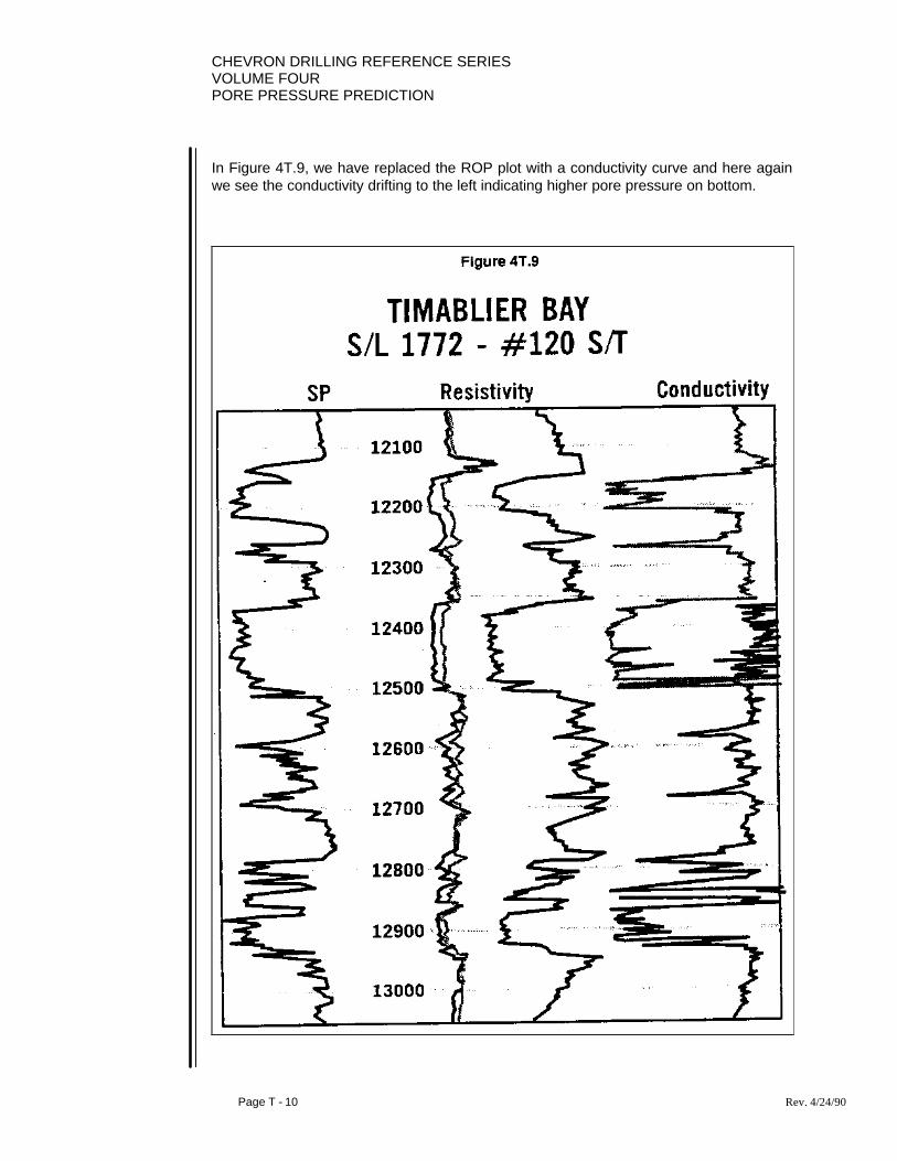
CHEVRON DRILLING REFERENCE SERIESVOLUME FOURPORE PRESSURE PREDICTION
Page T - 10 Rev. 4/24/90
In Figure 4T.9, we have replaced the ROP plot with a conductivity curve and here againwe see the conductivity drifting to the left indicating higher pore pressure on bottom.
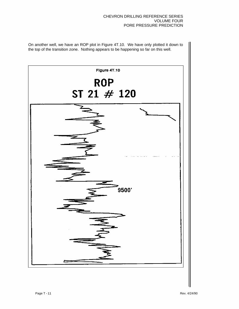
CHEVRON DRILLING REFERENCE SERIESVOLUME FOUR
PORE PRESSURE PREDICTION
Page T - 11 Rev. 4/24/90
On another well, we have an ROP plot in Figure 4T.10. We have only plotted it down tothe top of the transition zone. Nothing appears to be happening so far on this well.

CHEVRON DRILLING REFERENCE SERIESVOLUME FOUR
PORE PRESSURE PREDICTION
Page T - 13 Rev. 4/24/90
In Figure 4T.11, we look a little deeper on the electric log, and see a dramatic drift to theleft in resistivity and conductivity, illustrating a fairly significant transition zone. If wereplaced the conductivity curve with an ROP plot, we see the ROP drifting to the leftsignificantly in that shale section on bottom, indicating that pore pressures are increasing.
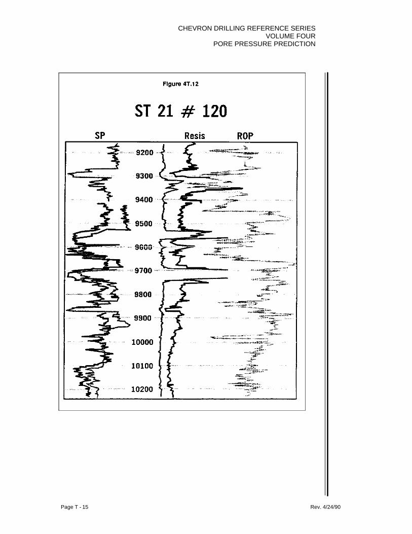
CHEVRON DRILLING REFERENCE SERIESVOLUME FOUR
PORE PRESSURE PREDICTION
Page T - 15 Rev. 4/24/90
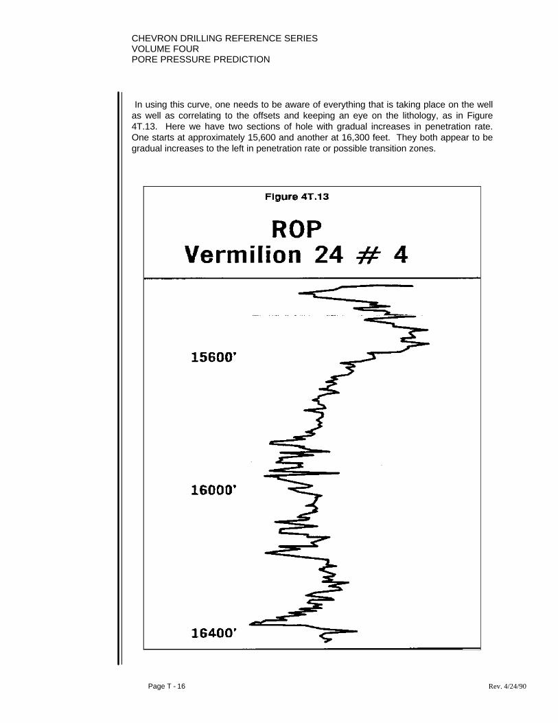
CHEVRON DRILLING REFERENCE SERIESVOLUME FOURPORE PRESSURE PREDICTION
Page T - 16 Rev. 4/24/90
In using this curve, one needs to be aware of everything that is taking place on the wellas well as correlating to the offsets and keeping an eye on the lithology, as in Figure4T.13. Here we have two sections of hole with gradual increases in penetration rate.One starts at approximately 15,600 and another at 16,300 feet. They both appear to begradual increases to the left in penetration rate or possible transition zones.

CHEVRON DRILLING REFERENCE SERIESVOLUME FOUR
PORE PRESSURE PREDICTION
Page T - 17 Rev. 4/24/90
As it turns out, the interval at 15,600 was a section of hole where gradual additions ofdiesel to the mud from 0% to 4% took place. This increasing penetration rate was due tothe additions of diesel as used as a drilling lubricant. The interval at 16,300 is alithological effect as we see illustrated in Figure 4T.14. The character of the sand is astair step effect out to the left as noted on both the Gamma Ray and the Conductivity.
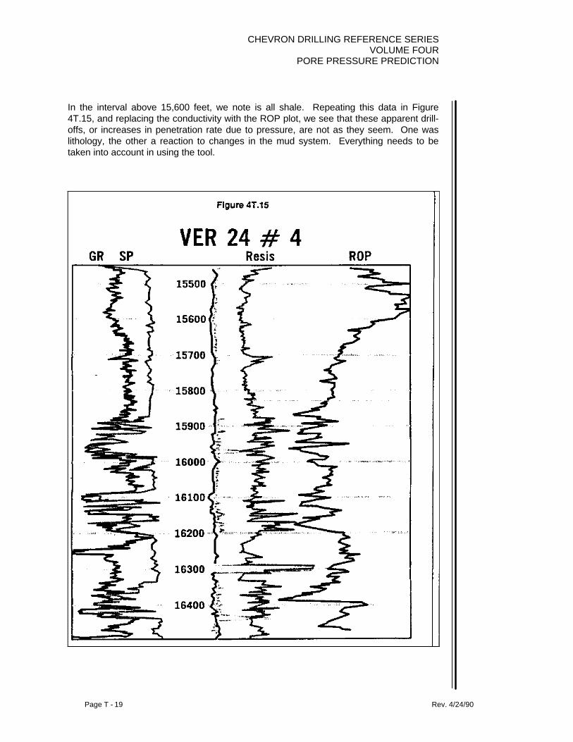
CHEVRON DRILLING REFERENCE SERIESVOLUME FOUR
PORE PRESSURE PREDICTION
Page T - 19 Rev. 4/24/90
In the interval above 15,600 feet, we note is all shale. Repeating this data in Figure4T.15, and replacing the conductivity with the ROP plot, we see that these apparent drill-offs, or increases in penetration rate due to pressure, are not as they seem. One waslithology, the other a reaction to changes in the mud system. Everything needs to betaken into account in using the tool.

CHEVRON DRILLING REFERENCE SERIESVOLUME FOURPORE PRESSURE PREDICTION
Page T - 20 Rev. 4/24/90
Another ROP plot appears in Figure 4T.16. Here at the bottom of this well we have agradual increase in penetration rate to the left below 11,200 ft.
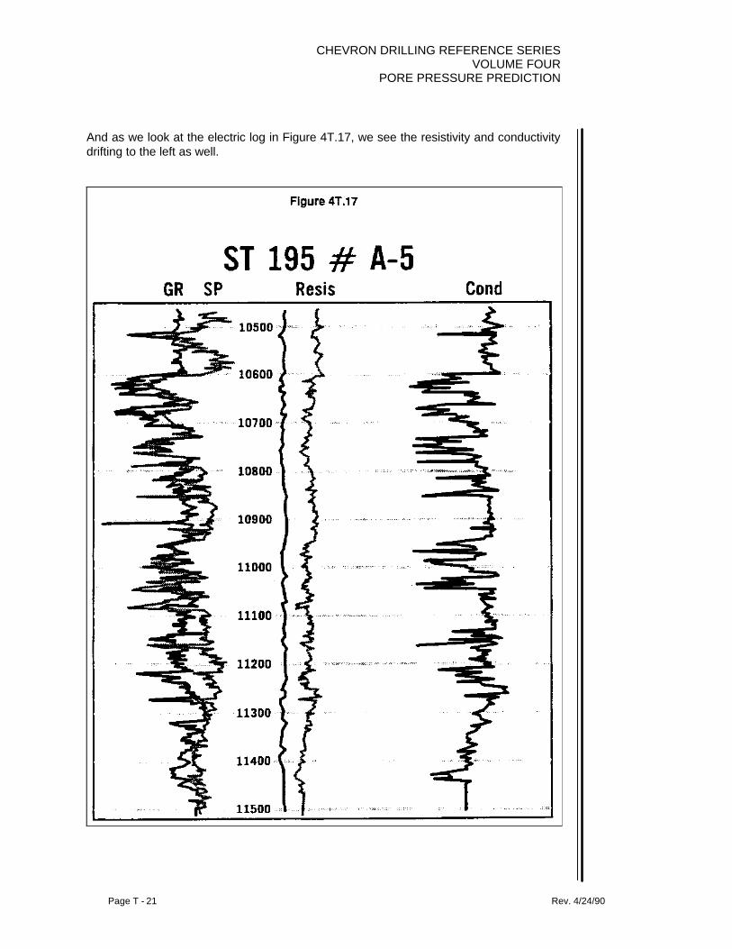
CHEVRON DRILLING REFERENCE SERIESVOLUME FOUR
PORE PRESSURE PREDICTION
Page T - 21 Rev. 4/24/90
And as we look at the electric log in Figure 4T.17, we see the resistivity and conductivitydrifting to the left as well.
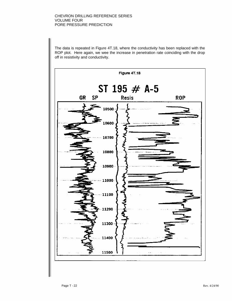
CHEVRON DRILLING REFERENCE SERIESVOLUME FOURPORE PRESSURE PREDICTION
Page T - 22 Rev. 4/24/90
The data is repeated in Figure 4T.18, where the conductivity has been replaced with theROP plot. Here again, we wee the increase in penetration rate coinciding with the dropoff in resistivity and conductivity.

CHEVRON DRILLING REFERENCE SERIESVOLUME FOUR
PORE PRESSURE PREDICTION
Page T - 23 Rev. 4/24/90
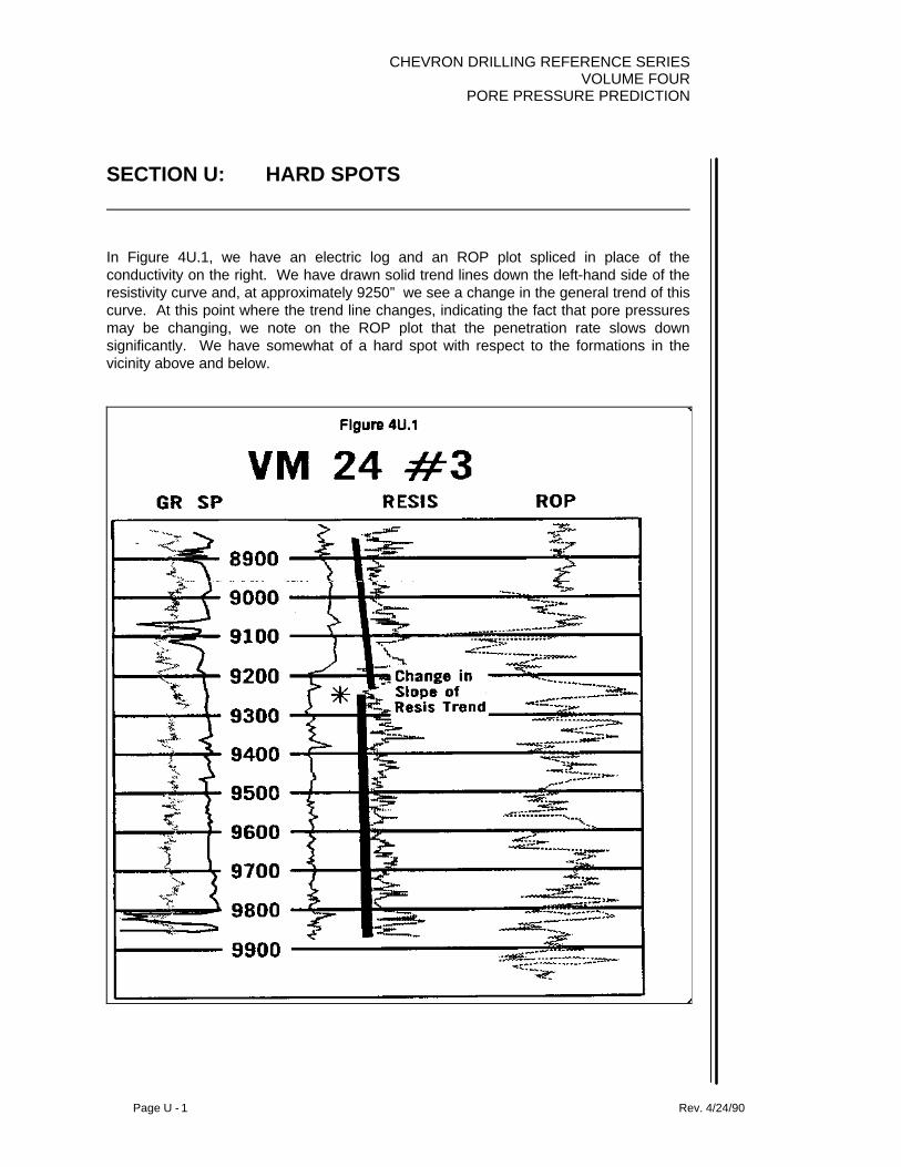
CHEVRON DRILLING REFERENCE SERIESVOLUME FOUR
PORE PRESSURE PREDICTION
Page U - 1 Rev. 4/24/90
SECTION U: HARD SPOTS
In Figure 4U.1, we have an electric log and an ROP plot spliced in place of theconductivity on the right. We have drawn solid trend lines down the left-hand side of theresistivity curve and, at approximately 9250” we see a change in the general trend of thiscurve. At this point where the trend line changes, indicating the fact that pore pressuresmay be changing, we note on the ROP plot that the penetration rate slows downsignificantly. We have somewhat of a hard spot with respect to the formations in thevicinity above and below.

CHEVRON DRILLING REFERENCE SERIESVOLUME FOURPORE PRESSURE PREDICTION
Page U - 2 Rev. 4/24/90
Generally, any time we see a change in the resistivity trend, it can indicate either the topof pressure, or within an abnormally pressured section, a point where the rate ofpressure building has changed. For example, if pore pressures were building one-halfpound per gallon every 100 feet and then started to build one pound per gallon every 100feet, this would be an inflection point or a point at which the trend would change as wellas a point where you would tend to see some hard or slow drilling. This is not to say thatall hard spots will mean a change in pressure, however, most changes in pressure will beaccompanied by a hard spot. This hard spot generally can only be recognized if usingthis or some other exaggerated ROP scale.
In Figure 4U.2, we are deeper in the same well. We note a significant shift in the trend inthe vicinity of 10,100 feet, and as we look at the ROP plot, we see a significant hard orslow spot.
CHEVRON DRILLING REFERENCE SERIESVOLUME FOUR
PORE PRESSURE PREDICTION
Page U - 3 Rev. 4/24/90
Additional examples in the same well as we go deeper appear here in Figures 4U.3 and4U.4, and again we see that as the trend changes or the rate at which pressure isbuilding changes, we have associated hard spots and this can be used as an indicator orsomething to keep an eye on as we drill the well.

CHEVRON DRILLING REFERENCE SERIESVOLUME FOURPORE PRESSURE PREDICTION
Page U - 4 Rev. 4/24/90

CHEVRON DRILLING REFERENCE SERIESVOLUME FOUR
PORE PRESSURE PREDICTION
Page U - 5 Rev. 4/24/90

CHEVRON DRILLING REFERENCE SERIESVOLUME FOURPORE PRESSURE PREDICTION
Page U - 6 Rev. 4/24/90
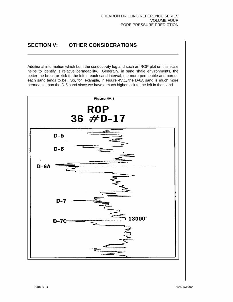
CHEVRON DRILLING REFERENCE SERIESVOLUME FOUR
PORE PRESSURE PREDICTION
Page V - 1 Rev. 4/24/90
SECTION V: OTHER CONSIDERATIONS
Additional information which both the conductivity log and such an ROP plot on this scalehelps to identify is relative permeability. Generally, in sand shale environments, thebetter the break or kick to the left in each sand interval, the more permeable and porouseach sand tends to be. So, for example, in Figure 4V.1, the D-6A sand is much morepermeable than the D-6 sand since we have a much higher kick to the left in that sand.
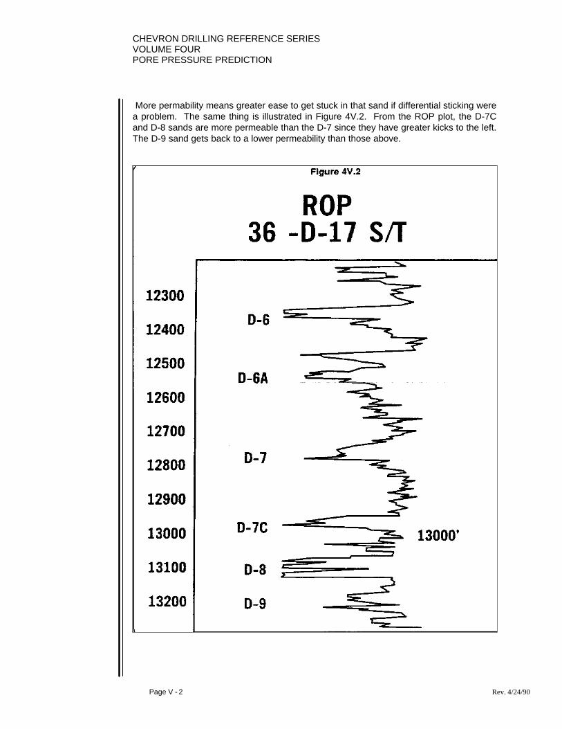
CHEVRON DRILLING REFERENCE SERIESVOLUME FOURPORE PRESSURE PREDICTION
Page V - 2 Rev. 4/24/90
More permability means greater ease to get stuck in that sand if differential sticking werea problem. The same thing is illustrated in Figure 4V.2. From the ROP plot, the D-7Cand D-8 sands are more permeable than the D-7 since they have greater kicks to the left.The D-9 sand gets back to a lower permeability than those above.
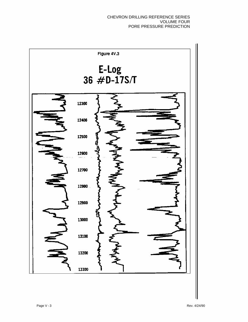
CHEVRON DRILLING REFERENCE SERIESVOLUME FOUR
PORE PRESSURE PREDICTION
Page V - 3 Rev. 4/24/90
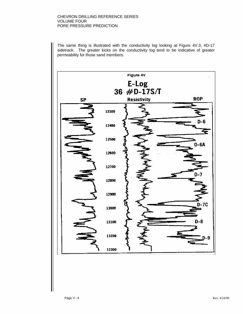
CHEVRON DRILLING REFERENCE SERIESVOLUME FOURPORE PRESSURE PREDICTION
Page V - 4 Rev. 4/24/90
The same thing is illustrated with the conductivity log looking at Figure 4V.3, #D-17sidetrack. The greater kicks on the conductivity log tend to be indicative of greaterpermeability for those sand members.

CHEVRON DRILLING REFERENCE SERIESVOLUME FOUR
PORE PRESSURE PREDICTION
Page V - 5 Rev. 4/24/90
This is not always true but the majority of the time when dealing with sand shaleenvironments, in wet sands, the conductivity curve, as well as the ROP plot will be apermeability or porosity indicator. In the illustration in Figure 4V.4, note how well theROP plot takes the place of the conductivity curve in the previous Figure.
Note also that significant changes in lithology are picked up as in Figure 4V.5. On thesidetrack hole, we have picked up a D-8 sand which was shaled-out down in the originalhole, and note some sands are more or less permeable than they were in the originalhole.
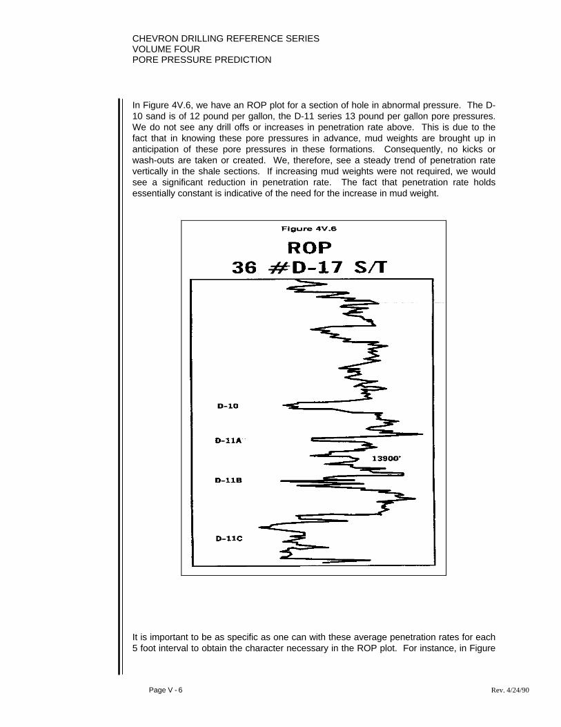
CHEVRON DRILLING REFERENCE SERIESVOLUME FOURPORE PRESSURE PREDICTION
Page V - 6 Rev. 4/24/90
In Figure 4V.6, we have an ROP plot for a section of hole in abnormal pressure. The D-10 sand is of 12 pound per gallon, the D-11 series 13 pound per gallon pore pressures.We do not see any drill offs or increases in penetration rate above. This is due to thefact that in knowing these pore pressures in advance, mud weights are brought up inanticipation of these pore pressures in these formations. Consequently, no kicks orwash-outs are taken or created. We, therefore, see a steady trend of penetration ratevertically in the shale sections. If increasing mud weights were not required, we wouldsee a significant reduction in penetration rate. The fact that penetration rate holdsessentially constant is indicative of the need for the increase in mud weight.
It is important to be as specific as one can with these average penetration rates for each5 foot interval to obtain the character necessary in the ROP plot. For instance, in Figure

CHEVRON DRILLING REFERENCE SERIESVOLUME FOUR
PORE PRESSURE PREDICTION
Page V - 7 Rev. 4/24/90
4V.7, penetration rates for joints of drill pipe have been averaged out. We, therefore, geta very blocky ROP plot which may make correlations much more difficult. It is better toaverage out each specific 5 foot interval and develop as much character in the curve aspossible.

CHEVRON DRILLING REFERENCE SERIESVOLUME FOURPORE PRESSURE PREDICTION
Page V - 8 Rev. 4/24/90
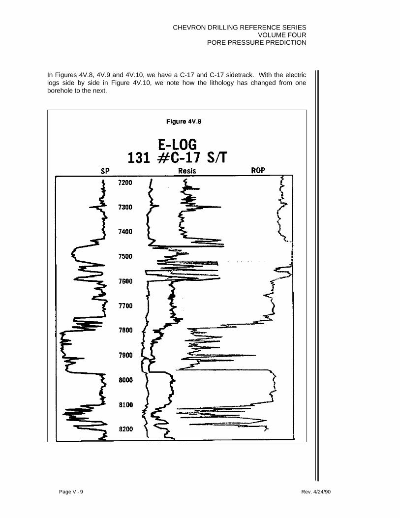
CHEVRON DRILLING REFERENCE SERIESVOLUME FOUR
PORE PRESSURE PREDICTION
Page V - 9 Rev. 4/24/90
In Figures 4V.8, 4V.9 and 4V.10, we have a C-17 and C-17 sidetrack. With the electriclogs side by side in Figure 4V.10, we note how the lithology has changed from oneborehole to the next.

CHEVRON DRILLING REFERENCE SERIESVOLUME FOURPORE PRESSURE PREDICTION
Page V - 10 Rev. 4/24/90

CHEVRON DRILLING REFERENCE SERIESVOLUME FOUR
PORE PRESSURE PREDICTION
Page V - 11 Rev. 4/24/90

CHEVRON DRILLING REFERENCE SERIESVOLUME FOURPORE PRESSURE PREDICTION
Page V - 12 Rev. 4/24/90

CHEVRON DRILLING REFERENCE SERIESVOLUME FOUR
PORE PRESSURE PREDICTION
Page V - 13 Rev. 4/24/90
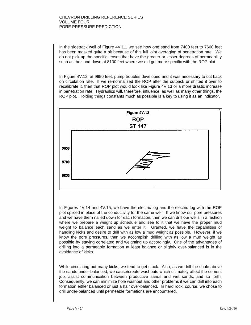
CHEVRON DRILLING REFERENCE SERIESVOLUME FOURPORE PRESSURE PREDICTION
Page V - 14 Rev. 4/24/90
In the sidetrack well of Figure 4V.11, we see how one sand from 7400 feet to 7600 feethas been masked quite a bit because of this full joint averaging of penetration rate. Wedo not pick up the specific lenses that have the greater or lesser degrees of permeabilitysuch as the sand down at 8100 feet where we did get more specific with the ROP plot.
In Figure 4V.12, at 9650 feet, pump troubles developed and it was necessary to cut backon circulation rate. If we re-normalized the ROP after the cutback or shifted it over torecalibrate it, then that ROP plot would look like Figure 4V.13 or a more drastic increasein penetration rate. Hydraulics will, therefore, influence, as well as many other things, theROP plot. Holding things constants much as possible is a key to using it as an indicator.
In Figures 4V.14 and 4V.15, we have the electric log and the electric log with the ROPplot spliced in place of the conductivity for the same well. If we know our pore pressuresand we have them nailed down for each formation, then we can drill our wells in a fashionwhere we prepare a weight up schedule and see to it that we have the proper mudweight to balance each sand as we enter it. Granted, we have the capabilities ofhandling kicks and desire to drill with as low a mud weight as possible. However, if weknow the pore pressures, then we accomplish drilling with as low a mud weight aspossible by staying correlated and weighting up accordingly. One of the advantages ofdrilling into a permeable formation at least balance or slightly over-balanced is in theavoidance of kicks.
While circulating out many kicks, we tend to get stuck. Also, as we drill the shale abovethe sands under-balanced, we cause/create washouts which ultimately affect the cementjob, assist communication between productive sands and wet sands, and so forth.Consequently, we can minimize hole washout and other problems if we can drill into eachformation either balanced or just a hair over-balanced. In hard rock, course, we chose todrill under-balanced until permeable formations are encountered.

CHEVRON DRILLING REFERENCE SERIESVOLUME FOUR
PORE PRESSURE PREDICTION
Page V - 15 Rev. 4/24/90
Figure 4V.14
As an example of how problems can arise, in Figure 4V.16, we have an ROP plot for awell where we drilled into a formation with an 11 or ppg mud and took an 11.4 ppgequivalent quick, ECD was not sufficient to control BHP, so it was, therefore, necessaryto circulate out on the choke. During the course of circulating out of the kick, troubledeveloped with both rig pumps, one pump on the cementing unit, and two jets on the bitplugged. This resulted in 36 hours to circulate out this kick. Many problems can arise atthe wrong time. Even if a kick is easily circulated out, there is a disadvantage in thewashouts created, and the wasted costly rig time.

CHEVRON DRILLING REFERENCE SERIESVOLUME FOURPORE PRESSURE PREDICTION
Page V - 16 Rev. 4/24/90
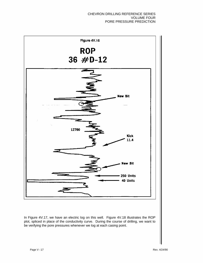
CHEVRON DRILLING REFERENCE SERIESVOLUME FOUR
PORE PRESSURE PREDICTION
Page V - 17 Rev. 4/24/90
In Figure 4V.17, we have an electric log on this well. Figure 4V.18 illustrates the ROPplot, spliced in place of the conductivity curve. During the course of drilling, we want tobe verifying the pore pressures whenever we log at each casing point.

CHEVRON DRILLING REFERENCE SERIESVOLUME FOURPORE PRESSURE PREDICTION
Page V - 18 Rev. 4/24/90
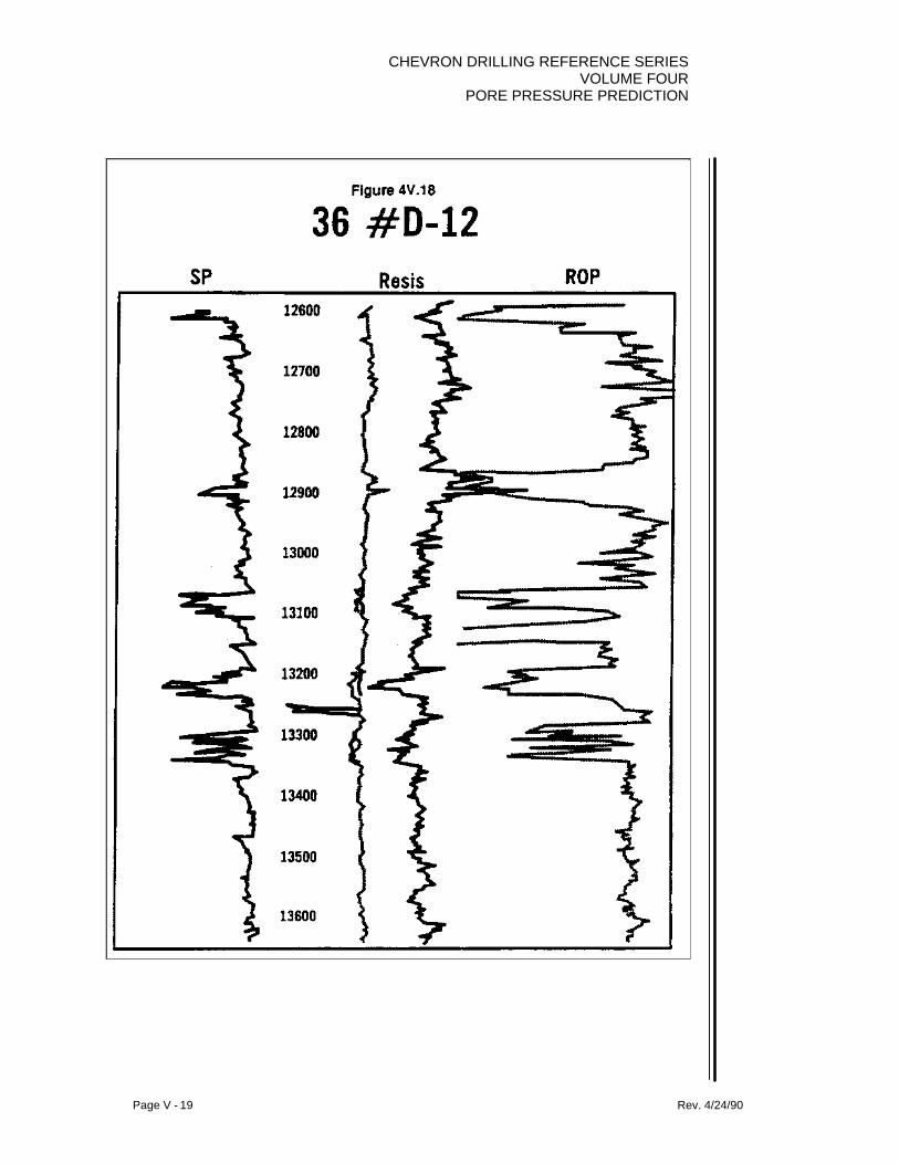
CHEVRON DRILLING REFERENCE SERIESVOLUME FOUR
PORE PRESSURE PREDICTION
Page V - 19 Rev. 4/24/90

CHEVRON DRILLING REFERENCE SERIESVOLUME FOURPORE PRESSURE PREDICTION
Page V - 20 Rev. 4/24/90
This can aid in the avoidance of many other problems, as well. For instance, in Figure4V.19, we have a productive sand at 5250 feet. This sand was drilled with a 9.5 poundper gallon mud. It is natural to assume being as shallow as it is, and being drilled with a9.5 ppg mud, it to be a normally pressured or a nine pound per gallon equivalent porepressure. However, in plotting the logs, it turns out, this sand is a 9.5 pound per gallonpore pressure.
In testing the well, the sand was perforated with a wire line casing gun with a 9.5 ppgclear brine in the hole. Due to temperature expansion of the brine, the effective weight atTD was less than 9.5 pounds per gallon. All brines do experience thermal expansion andultimately will have a reduced hydrostatic head due to this expansion. It would,therefore, be necessary to know that this formation is of 9.5 pound per gallon porepressure and realize that something greater than 9.5 ppg would be necessary.

CHEVRON DRILLING REFERENCE SERIESVOLUME FOUR
PORE PRESSURE PREDICTION
Page V - 21 Rev. 4/24/90