Vivaldi: A Decentralized Network Coordinate System

Frank Dabek, Russ Cox, Frans Kaashoek, Robert MorrisMIT CSAIL

Cambridge, MA

fdabek,rsc,kaashoek,rtm@mit.edu

ABSTRACTLarge-scale Internet applications can benefit from an ability to pre-dict round-trip times to other hosts without having to contact themfirst. Explicit measurements are often unattractive because the costof measurement can outweigh the benefits of exploiting proximityinformation. Vivaldi is a simple, light-weight algorithm that as-signs synthetic coordinates to hosts such that the distance betweenthe coordinates of two hosts accurately predicts the communicationlatency between the hosts.

Vivaldi is fully distributed, requiring no fixed network infrastruc-ture and no distinguished hosts. It is also efficient: a new host cancompute good coordinates for itself after collecting latency infor-mation from only a few other hosts. Because it requires little com-munication, Vivaldi can piggy-back on the communication patternsof the application using it and scale to a large number of hosts.

An evaluation of Vivaldi using a simulated network whose laten-cies are based on measurements among 1740 Internet hosts showsthat a 2-dimensional Euclidean model with height vectors embedsthese hosts with low error (the median relative error in round-triptime prediction is 11 percent).

Categories and Subject DescriptorsC.2.1 [Computer Communication Networks]: Network Archi-tecture and Design—Network topology; C.2.5 [Computer Com-munication Networks]: Local and Wide-Area Networks—Inter-net

General TermsAlgorithms, Measurement, Performance, Design, Experimentation

KeywordsVivaldi, network coordinates, Internet topology

1. INTRODUCTIONSynthetic coordinate systems [3,17,19,26] allow an Internet host

to predict the round-trip latencies to other hosts. Hosts compute

Permission to make digital or hard copies of all or part of this work forpersonal or classroom use is granted without fee provided that copies arenot made or distributed for profit or commercial advantage and that copiesbear this notice and the full citation on the first page. To copy otherwise, torepublish, to post on servers or to redistribute to lists, requires prior specificpermission and/or a fee.SIGCOMM’04, Aug. 30–Sept. 3, 2004, Portland, Oregon, USA.Copyright 2004 ACM 1-58113-862-8/04/0008 ...$5.00.

synthetic coordinates in some coordinate space such that distancebetween two hosts’ synthetic coordinates predicts the RTT betweenthem in the Internet. Thus, if a host x learns the coordinates of ahost y, x doesn’t have to perform an explicit measurement to de-termine the RTT to y; instead, the distance between x and y in thecoordinate space is an accurate predictor of the RTT.

The Internet’s properties determine whether synthetic coordi-nates are likely to work well. For example, if Internet latency isdominated by speed-of-light delay over links, and the Internet iswell-enough connected that there is a roughly direct physical pathbetween every pair of hosts, and the Internet routing system findsthese direct paths, then synthetic coordinates that mimic latitudeand longitude are likely to predict latency well.

Unfortunately, these properties are only approximate. Packetsoften deviate from great-circle routes because few site pairs are di-rectly connected, because different ISPs peer at a limited number oflocations, and because transmission time and router electronics de-lay packets. The resulting distorted latencies make it impossible tochoose two-dimensional host coordinates that predict latency per-fectly, so a synthetic coordinate system must have a strategy forchoosing coordinates that minimize prediction errors. In addition,coordinates need not be limited to two dimensions; Vivaldi is ableto eliminate certain errors by augmenting coordinates with a height.

The ability to predict RTT without prior communication allowssystems to use proximity information for better performance withless measurement overhead than probing. A coordinate system canbe used to select which of a number of replicated servers to fetch adata item from; coordinates are particularly helpful when the num-ber of potential servers is large or the amount of data is small. In ei-ther case it would not be practical to first probe all the servers to findthe closest, since the cost of the probes would outweigh the benefitof an intelligent choice. Content distribution and file-sharing sys-tems such as KaZaA [12], BitTorrent [1], and CoDeeN [31] areexamples of systems that offer a large number of replica servers.CFS [6] and DNS [13] are examples of systems that offer modestnumbers of replicas, but each piece of data is small. All of theseapplications could benefit from network coordinates.

Designing a synthetic coordinate system for use in large-scaledistributed Internet applications involves the following challenges:

• Finding a metric space that embeds the Internet with littleerror. A suitable space must cope with the difficulties intro-duced by Internet routing, transmission time, and queuing.

• Scaling to a large number of hosts. Synthetic coordinate sys-tems are of most value in large-scale applications; if only fewhosts are involved, direct measurement of RTT is practical.

• Decentralizing the implementation. Many emerging applica-tions, such as peer-to-peer applications, are distributed and

symmetric in nature and do not inherently have special, reli-able hosts that are candidates for landmarks.

• Minimizing probe traffic. An ideal synthetic coordinate sys-tem would not introduce any additional network traffic, butwould be able to gather whatever information it needed fromthe application’s existing communication.

• Adapting to changing network conditions. The relative loca-tion of a host in a network may change due to congestion oreven reconfiguration of the network. The system should beable to adjust the coordinates of hosts periodically to respondto these changes.

A number of existing synthetic coordinate systems address someof these challenges, but none addresses them all, as Section 6 dis-cusses.

The primary contribution of this paper is a decentralized, low-overhead, adaptive synthetic coordinate system, Vivaldi, that com-putes coordinates which predict Internet latencies with low error.Vivaldi was developed for and is used by the Chord peer-to-peerlookup system which uses coordinates to avoid contacting distanthosts when performing a lookup [7].

This paper extends earlier descriptions of Vivaldi [4, 5] and con-siders new variations, particularly a coordinate space that includesthe notion of a directionless height that improves the prediction ac-curacy of the system on data sets derived from measurements ofthe Internet. Height is included to capture transmission delays onthe access links of single-homed hosts. A detailed evaluation usinga simulator driven with actual Internet latencies between 1740 In-ternet hosts shows that Vivaldi achieves errors as low as GNP [17],a landmark-based coordinate system, even though Vivaldi has nonotion of landmarks.

A further contribution of this paper is that coordinates drawnfrom a two-dimensional Euclidean model with a height can accu-rately predict latency between the 1740 Internet hosts. Simulationsshow that this model is better than 2- or 3-dimensional Euclideanmodels or a spherical model. These findings suggest that the fol-lowing properties hold in the data set: inter-host RTT is dominatedby geographic distance, the Internet core does not “wrap around”the Earth to any significant extent, and the time required to traversean access-link is often a significant fraction of total RTT.

The rest of this paper is organized as follows. Section 2 presentsthe Vivaldi algorithm. Section 3 describes the methodology forevaluating Vivaldi. Section 4 presents the results from evaluatingVivaldi. Section 5 investigates different models to embed the In-ternet. Section 6 discusses the related work that led us to Vivaldi.Finally, section 7 summarizes our conclusions.

2. ALGORITHMVivaldi assigns each host synthetic coordinates in a coordinate

space, attempting to assign coordinates such that the distance in thecoordinate space between two hosts accurately predicts the packettransmission RTT between the hosts. No low-dimensional coordi-nate space would allow Vivaldi to predict RTTs between Internethosts exactly, because, for example, Internet latencies violate thetriangle inequality. The algorithm instead attempts to find coordi-nates that minimize the error of predictions.

We first describe this prediction error in more detail and brieflydiscuss possible coordinate systems. Then, we show a simple cen-tralized algorithm that finds coordinates that minimize a squarederror function given complete knowledge of RTTs in the network.Then we present a simple distributed algorithm that computes co-ordinates based on measurements from each node to a few other

nodes. Finally, we refine this distributed algorithm to convergequickly to accurate coordinates.

2.1 Prediction errorLet Li j be the actual RTT between nodes i and j, and xi be the

coordinates assigned to node i. We can characterize the errors inthe coordinates using a squared-error function:

E =∑

i

∑

j

(

Li j −∥

∥

∥xi − x j

∥

∥

∥

)2(1)

where∥

∥

∥xi − x j

∥

∥

∥ is the distance between the coordinates of nodes iand j in the chosen coordinate space. Other systems choose to min-imize a different quantity; PIC [3], for instance, minimizes squaredrelative error. We chose the squared error function because it hasan analogue to the displacement in a physical mass-spring system:minimizing the energy in a spring network is equivalent to mini-mizing the squared-error function.

2.2 Synthetic coordinate structureAlgorithms can choose the structure of coordinates and the dis-

tance function that determines the predicted latency given two co-ordinates. Coordinates should be compact and it should be easy tocompute an RTT prediction given two coordinates. The simplestchoice is to use n-dimensional coordinates with the standard Eu-clidean distance function. Spherical, toroidal, hyperbolic and othercoordinate structures have also been proposed (e.g., [27]). Thesecoordinate systems use alternative distance functions in the hopethat they predict latency better. Section 5 will present the height-vector coordinates that we propose. In the remainder of this section,however, we will present algorithms that work with any coordinatesystem that supports the magnitude, addition, and subtraction oper-ations.

2.3 Centralized algorithmWe first describe a simple, centralized algorithm than can mini-

mize Equation 1. Vivaldi is a distributed version of this algorithm.Given our choice of E, simulating of a network of physical springsproduces coordinates that minimize E.

Conceptually, this minimization places a spring between eachpair of nodes (i, j) with a rest length set to the known RTT (Li j).The current length of the spring is considered to be the distancebetween the nodes in the coordinate space. The potential energy ofsuch a spring is proportional to the square of the displacement fromits rest length: the sum of these energies over all springs is exactlythe error function we want to minimize.

Since the squared-error function is equivalent to spring energy,we can minimize it by simulating the movements of nodes underthe spring forces. While the minimum energy configuration of thespring system corresponds to the minimum error coordinate assign-ment, it is not guaranteed that the simulation will find this globalminimum: the system may come to rest in a local minimum.

This approach to minimization mirrors work on model recon-struction [11] and a similar recent coordinate approach using forcefields [26].

We will now describe the centralized algorithm more precisely.Define Fi j to be the force vector that the spring between nodes iand j exerts on node i. From Hooke’s law we can show that F is:

Fi j =(

Li j −∥

∥

∥xi − x j

∥

∥

∥

)

× u(xi − x j).

The scalar quantity(

Li j −∥

∥

∥xi − x j

∥

∥

∥

)

is the displacement of thespring from rest. This quantity gives the magnitude of the force ex-

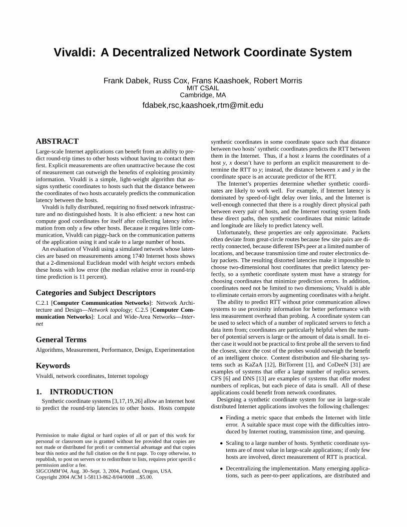
// Input: latency matrix and initial coordinates// Output: more accurate coordinates in xcompute coordinates(L, x)

while (error (L, x) > tolerance)foreach i

F = 0foreach j// Compute error/force of this spring. (1)e = Li j − ‖xi − x j‖

// Add the force vector of this spring to the total force. (2)F = F + e × u(xi − x j)

// Move a small step in the direction of the force. (3)xi = xi + t × F

Figure 1: The centralized algorithm.

erted by the spring on i and j (we will ignore the spring constant).The unit vector u(xi − x j) gives the direction of the force on i. Scal-ing this vector by the force magnitude calculated above gives theforce vector that the spring exerts on node i.

The net force on i (Fi) is the sum of the forces from other nodes:

Fi =∑

j,i

Fi j.

To simulate the spring network’s evolution the algorithm consid-ers small intervals of time. At each interval, the algorithm moveseach node (xi) a small distance in the coordinate space in the direc-tion of Fi and then recomputes all the forces. The coordinates atthe end of a time interval are:

xi = xi + Fi × t,

where t is the length of the time interval. The size of t determineshow far a node moves at each time interval. Finding an appropriatet is important in the design of Vivaldi.

Figure 1 presents the pseudocode for the centralized algorithm.For each node i in the system, compute coordinates computes theforce on each spring connected to i (line 1) and adds that forceto the total force on i (line 2). After all of the forces have beenadded together, i moves a small distance in the direction of theforce (line 3). This process is repeated until the system convergesto coordinates that predict error well.

This centralized algorithm (and the algorithms that will build onit) finds coordinates that minimize squared error because the forcefunction we chose (Hooke’s law) defines a force that is proportionalto displacement. If we chose a different force function, a differenterror function would be minimized. For instance, if spring forcewere a constant regardless of displacement, this algorithm wouldminimize the sum of (unsquared) errors.

2.4 The simple Vivaldi algorithmThe centralized algorithm described in Section 2.3 computes co-

ordinates for all nodes given all RTTs. Here we extend the algo-rithm so that each node computes and continuously adjusts its co-ordinates based only on measured RTTs from the node to a handfulof other nodes and the current coordinates of those nodes.

Each node participating in Vivaldi simulates its own movementin the spring system. Each node maintains its own current coor-dinates, starting with coordinates at the origin. Whenever a nodecommunicates with another node, it measures the RTT to that nodeand also learns that node’s current coordinates.

The input to the distributed Vivaldi algorithm is a sequence of

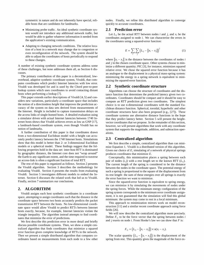
// Node i has measured node j to be rtt ms away,// and node j says it has coordinates x j.simple vivaldi(rtt, x j)// Compute error of this sample. (1)e = rtt − ‖xi − x j‖

// Find the direction of the force the error is causing. (2)dir = u(xi − x j)// The force vector is proportional to the error (3)f = dir × e// Move a a small step in the direction of the force. (4)xi = xi + δ × dir

Figure 2: The simple Vivaldi algorithm, with a constanttimestep δ.

such samples. In response to a sample, a node allows itself to bepushed for a short time step by the corresponding spring; each ofthese movements reduce the node’s error with respect to one othernode in the system. As nodes continually communicate with othernodes, they converge to coordinates that predict RTT well.

When node i with coordinates xi learns about node j with coor-dinates x j and measured RTT rtt, it updates its coordinates usingthe update rule:

xi = xi + δ ×(

rtt − ‖xi − x j‖)

× u(xi − x j).

This rule is identical to the individual forces calculated in theinner loop of the centralized algorithm.

Because all nodes start at the same location, Vivaldi must sep-arate them somehow. Vivaldi does this by defining u(0) to be aunit-length vector in a randomly chosen direction. Two nodes oc-cupying the same location will have a spring pushing them awayfrom each other in some arbitrary direction.

Figure 2 shows the pseudocode for this distributed algorithm.The simple vivaldi procedure is called whenever a new RTT mea-surement is available. simple vivaldi is passed an RTT measure-ment to the remote node and the remote node’s coordinates. Theprocedure first calculates the error in its current prediction to thetarget node (line 1). The node will move towards or away from thetarget node based on the magnitude of this error; lines 2 and 3 findthe direction (the force vector created by the algorithm’s imaginedspring) the node should move. Finally, the node moves a fractionof the distance to the target node in line 4, using a constant timestep(δ).

This algorithm effectively implements a weighted moving aver-age that is biased toward more recent samples. To avoid this bias,each node could maintain a list of every sample it has ever received,but since all nodes in the system are constantly updating their co-ordinates, old samples eventually become outdated. Further, main-taining such a list would not scale to systems with large numbersof nodes.

2.5 An adaptive timestepThe main difficulty in implementing Vivaldi is ensuring that it

converges to coordinates that predict RTT well. The rate of conver-gence is governed by the δ timestep: large δ values cause Vivaldi toadjust coordinates in large steps. However, if all Vivaldi nodes uselarge δ values, the result is typically oscillation and failure to con-verge to useful coordinates. Intuitively, a large δ causes nodes tojump back and forth across low energy valleys that a smaller deltawould explore.

An additional challenge is handling nodes that have a high error

in their coordinates. If a node n communicates with some nodethat has coordinates that predict RTTs badly, any update that nmakes based on those coordinates is likely to increase predictionerror rather than decrease it.

We would like to obtain both fast convergence and avoidance ofoscillation. Vivaldi does this by varying δ depending on how certainthe node is about its coordinates (we will discuss how a node main-tains an estimate of the accuracy of its coordinates in Section 2.6).When a node is still learning its rough place in the network (as hap-pens, for example, when the node first joins), larger values of δ willhelp it move quickly to an approximately correct position. Oncethere, smaller values of δ will help it refine its position.

A simple adaptive δ might use a constant fraction (cc < 1) of thenode’s estimated error:

δ = cc × local error

δ can be viewed as the fraction of the way the node is allowed tomove toward the perfect position for the current sample. If a nodepredicts its error to be within ±5%, then it won’t move more than5% toward a corrected position. On the other hand, if its error islarge (say, ±100%), then it will eagerly move all the way to thecorrected position.

A problem with setting δ to the prediction error is that it doesn’ttake into account the accuracy of the remote node’s coordinates. Ifthe remote node has an accuracy of ±50%, then it should be givenless credence than a remote node with an accuracy of ±5%. Vivaldiimplements this timestep:

δ = cc ×local error

local error + remote error(2)

Using this δ, an accurate node sampling an inaccurate node willnot move much, an inaccurate node sampling an accurate node willmove a lot, and two nodes of similar accuracy will split the differ-ence.

Computing the timestep in this way provides the properties wedesire: quick convergence, low oscillation, and resilience againsthigh-error nodes.

2.6 Estimating accuracyThe adaptive timestep described above requires that nodes have a

running estimate of how accurate their coordinates are. Each nodecompares each new measured RTT sample with the predicted RTT,and maintains a moving average of recent relative errors (absoluteerror divided by actual latency). As in the computation of δ, theweight of each sample is determined by the ratio between the pre-dicted relative error of the local node and of the node being sam-pled. In our experiments, the estimate is always within a smallconstant factor of the actual error. Finding more accurate and moreelegant error predictors is future work, but this rough predictionhas been sufficient to support the parts of the algorithm (such as thetimestep) that depend on it.

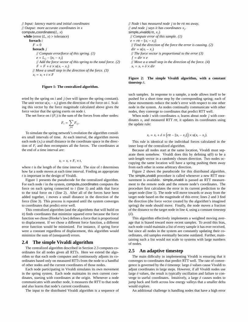
2.7 The Vivaldi algorithmFigure 3 shows pseudocode for Vivaldi. The vivaldi procedure

computes the weight of a sample based on local and remote error(line 1). The algorithm must also track the local relative error. Itdoes this using a weighted moving average (lines 2 and 3). The re-mainder of the Vivaldi algorithm is identical to the simple version.

Vivaldi is fully distributed: an identical vivaldi procedure runson every node. It is also efficient: each sample provides informa-tion that allows a node to update its coordinates. Because Vivaldiis constantly updating coordinates, it is reactive; if the underlying

// Incorporate new information: node j has been// measured to be rtt ms away, has coordinates x j,// and an error estimate of e j.//

// Our own coordinates and error estimate are xi and ei.//

// The constants ce and cc are tuning parameters.vivaldi(rtt, x j, e j)// Sample weight balances local and remote error. (1)w = ei/(ei + e j)

// Compute relative error of this sample. (2)es =∣

∣

∣‖xi − x j‖ − rtt∣

∣

∣/rtt

// Update weighted moving average of local error. (3)ei = es × ce × w + ei × (1 − ce × w)

// Update local coordinates. (4)δ = cc × wxi = xi + δ ×

(

rtt − ‖xi − x j‖)

× u(xi − x j)

Figure 3: The Vivaldi algorithm, with an adaptive timestep.

topology changes, nodes naturally update their coordinates accord-ingly. Finally, it handles high-error nodes. The next sections evalu-ate how well Vivaldi achieves these properties experimentally andinvestigate what coordinate space best fits the Internet.

3. EVALUATION METHODOLOGYThe experiments are conducted using a packet-level network sim-

ulator running with RTT data collected from the Internet. This sec-tion presents the details of the framework used for the experiments.

3.1 Latency dataThe Vivaldi simulations are driven by a matrix of inter-host In-

ternet RTTs; Vivaldi computes coordinates using a subset of theRTTs, and the full matrix is needed to evaluate the quality of pre-dictions made by those coordinates.

We use two different data sets derived from measurements of areal network. The first and smaller data set involves 192 hosts onthe PlanetLab network test bed [20]. These measurements weretaken from a public PlanetLab all-pairs-pings trace [28].

The second data set involves 1740 Internet DNS servers. Webuilt a tool based on the King method [10] to collect the full matrixof RTTs. To determine the distance between DNS server A andserver B, we first measure the round trip time to server A and thenask server A to recursively resolve a domain served by B. The dif-ference in times between the two operations yields an estimate ofthe round trip time between A and B (see Figure 4). Each queryinvolves a unique target name to suppress DNS caching.

We harvested the addresses of recursive DNS servers by ex-tracting the NS records for IP addresses of hosts participating ina Gnutella network. If a domain is served by multiple, geograph-ically diverse name servers, queries targeted at domain D (and in-tended for name server B) could be forwarded to a different nameserver, C, which also serves D. To avoid this error, we filtered thelist of target domains and name servers to include only those do-mains where all authoritative name servers are on the same subnet(i.e. the IP addresses of the name servers are identical except forthe low octet). We also verified that the target nameservers were re-sponsible for the associated names by performing a non-recursive

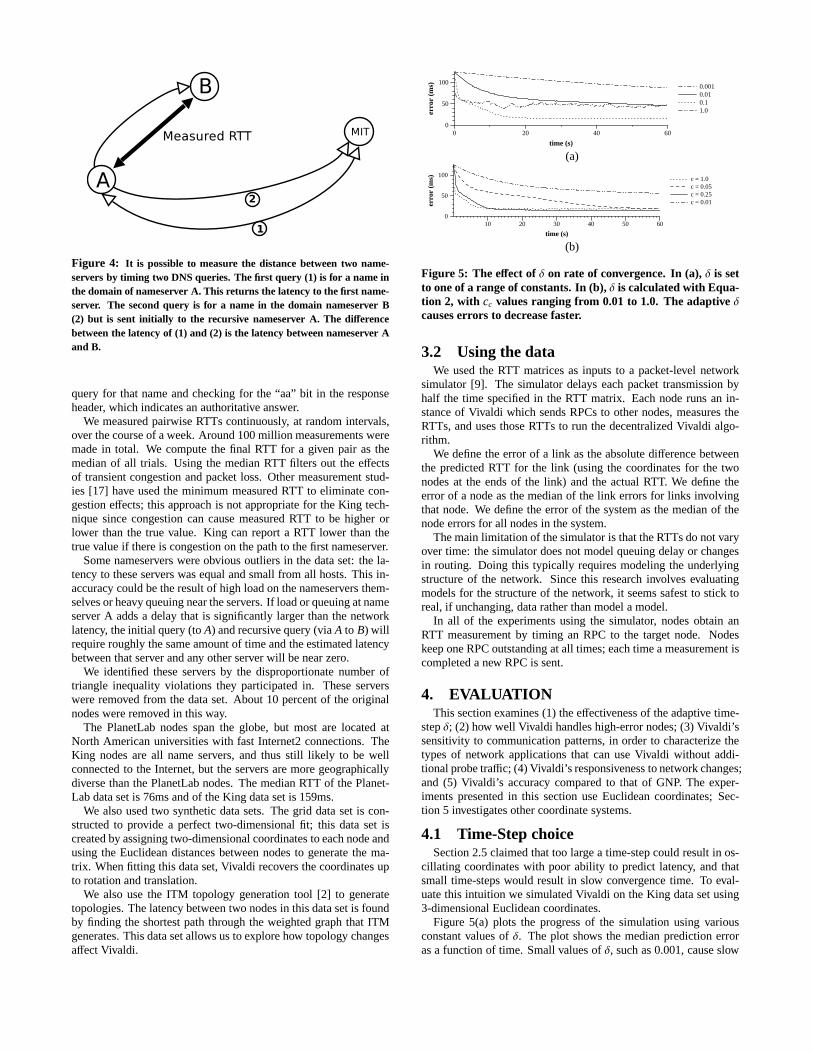
Figure 4: It is possible to measure the distance between two name-servers by timing two DNS queries. The first query (1) is for a name inthe domain of nameserver A. This returns the latency to the first name-server. The second query is for a name in the domain nameserver B(2) but is sent initially to the recursive nameserver A. The differencebetween the latency of (1) and (2) is the latency between nameserver Aand B.

query for that name and checking for the “aa” bit in the responseheader, which indicates an authoritative answer.

We measured pairwise RTTs continuously, at random intervals,over the course of a week. Around 100 million measurements weremade in total. We compute the final RTT for a given pair as themedian of all trials. Using the median RTT filters out the effectsof transient congestion and packet loss. Other measurement stud-ies [17] have used the minimum measured RTT to eliminate con-gestion effects; this approach is not appropriate for the King tech-nique since congestion can cause measured RTT to be higher orlower than the true value. King can report a RTT lower than thetrue value if there is congestion on the path to the first nameserver.

Some nameservers were obvious outliers in the data set: the la-tency to these servers was equal and small from all hosts. This in-accuracy could be the result of high load on the nameservers them-selves or heavy queuing near the servers. If load or queuing at nameserver A adds a delay that is significantly larger than the networklatency, the initial query (to A) and recursive query (via A to B) willrequire roughly the same amount of time and the estimated latencybetween that server and any other server will be near zero.

We identified these servers by the disproportionate number oftriangle inequality violations they participated in. These serverswere removed from the data set. About 10 percent of the originalnodes were removed in this way.

The PlanetLab nodes span the globe, but most are located atNorth American universities with fast Internet2 connections. TheKing nodes are all name servers, and thus still likely to be wellconnected to the Internet, but the servers are more geographicallydiverse than the PlanetLab nodes. The median RTT of the Planet-Lab data set is 76ms and of the King data set is 159ms.

We also used two synthetic data sets. The grid data set is con-structed to provide a perfect two-dimensional fit; this data set iscreated by assigning two-dimensional coordinates to each node andusing the Euclidean distances between nodes to generate the ma-trix. When fitting this data set, Vivaldi recovers the coordinates upto rotation and translation.

We also use the ITM topology generation tool [2] to generatetopologies. The latency between two nodes in this data set is foundby finding the shortest path through the weighted graph that ITMgenerates. This data set allows us to explore how topology changesaffect Vivaldi.

0 20 40 60

time (s)

0

50

100

erro

r (m

s) 0.0010.010.11.0

(a)

10 20 30 40 50 60

time (s)

0

50

100

erro

r (m

s) c = 1.0c = 0.05c = 0.25c = 0.01

(b)

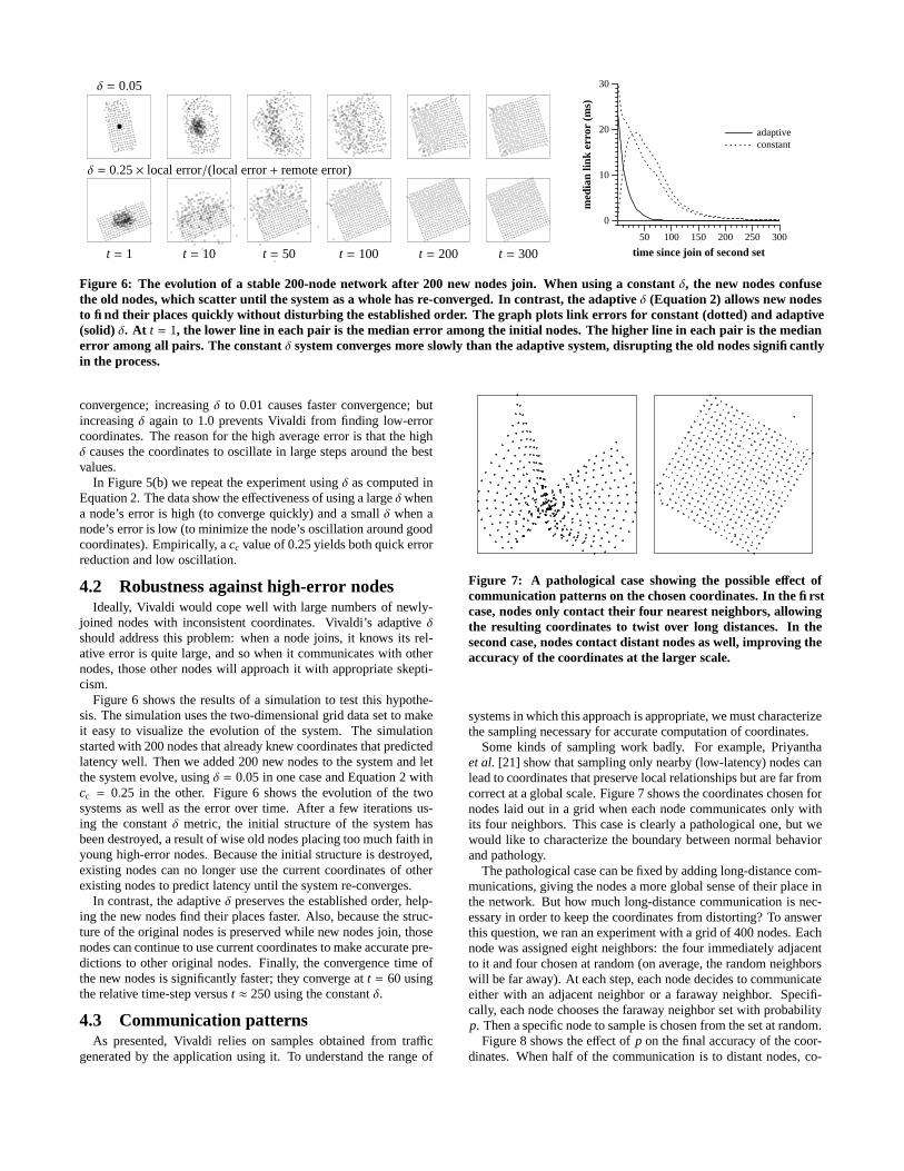
Figure 5: The effect of δ on rate of convergence. In (a), δ is setto one of a range of constants. In (b), δ is calculated with Equa-tion 2, with cc values ranging from 0.01 to 1.0. The adaptive δcauses errors to decrease faster.

3.2 Using the dataWe used the RTT matrices as inputs to a packet-level network

simulator [9]. The simulator delays each packet transmission byhalf the time specified in the RTT matrix. Each node runs an in-stance of Vivaldi which sends RPCs to other nodes, measures theRTTs, and uses those RTTs to run the decentralized Vivaldi algo-rithm.

We define the error of a link as the absolute difference betweenthe predicted RTT for the link (using the coordinates for the twonodes at the ends of the link) and the actual RTT. We define theerror of a node as the median of the link errors for links involvingthat node. We define the error of the system as the median of thenode errors for all nodes in the system.

The main limitation of the simulator is that the RTTs do not varyover time: the simulator does not model queuing delay or changesin routing. Doing this typically requires modeling the underlyingstructure of the network. Since this research involves evaluatingmodels for the structure of the network, it seems safest to stick toreal, if unchanging, data rather than model a model.

In all of the experiments using the simulator, nodes obtain anRTT measurement by timing an RPC to the target node. Nodeskeep one RPC outstanding at all times; each time a measurement iscompleted a new RPC is sent.

4. EVALUATIONThis section examines (1) the effectiveness of the adaptive time-

step δ; (2) how well Vivaldi handles high-error nodes; (3) Vivaldi’ssensitivity to communication patterns, in order to characterize thetypes of network applications that can use Vivaldi without addi-tional probe traffic; (4) Vivaldi’s responsiveness to network changes;and (5) Vivaldi’s accuracy compared to that of GNP. The exper-iments presented in this section use Euclidean coordinates; Sec-tion 5 investigates other coordinate systems.

4.1 Time-Step choiceSection 2.5 claimed that too large a time-step could result in os-

cillating coordinates with poor ability to predict latency, and thatsmall time-steps would result in slow convergence time. To eval-uate this intuition we simulated Vivaldi on the King data set using3-dimensional Euclidean coordinates.

Figure 5(a) plots the progress of the simulation using variousconstant values of δ. The plot shows the median prediction erroras a function of time. Small values of δ, such as 0.001, cause slow

δ = 0.05

δ = 0.25 × local error/(local error + remote error)

t = 1 t = 10 t = 50 t = 100 t = 200 t = 30050 100 150 200 250 300

time since join of second set

0

10

20

30

med

ian

link

erro

r (m

s)

adaptiveconstant

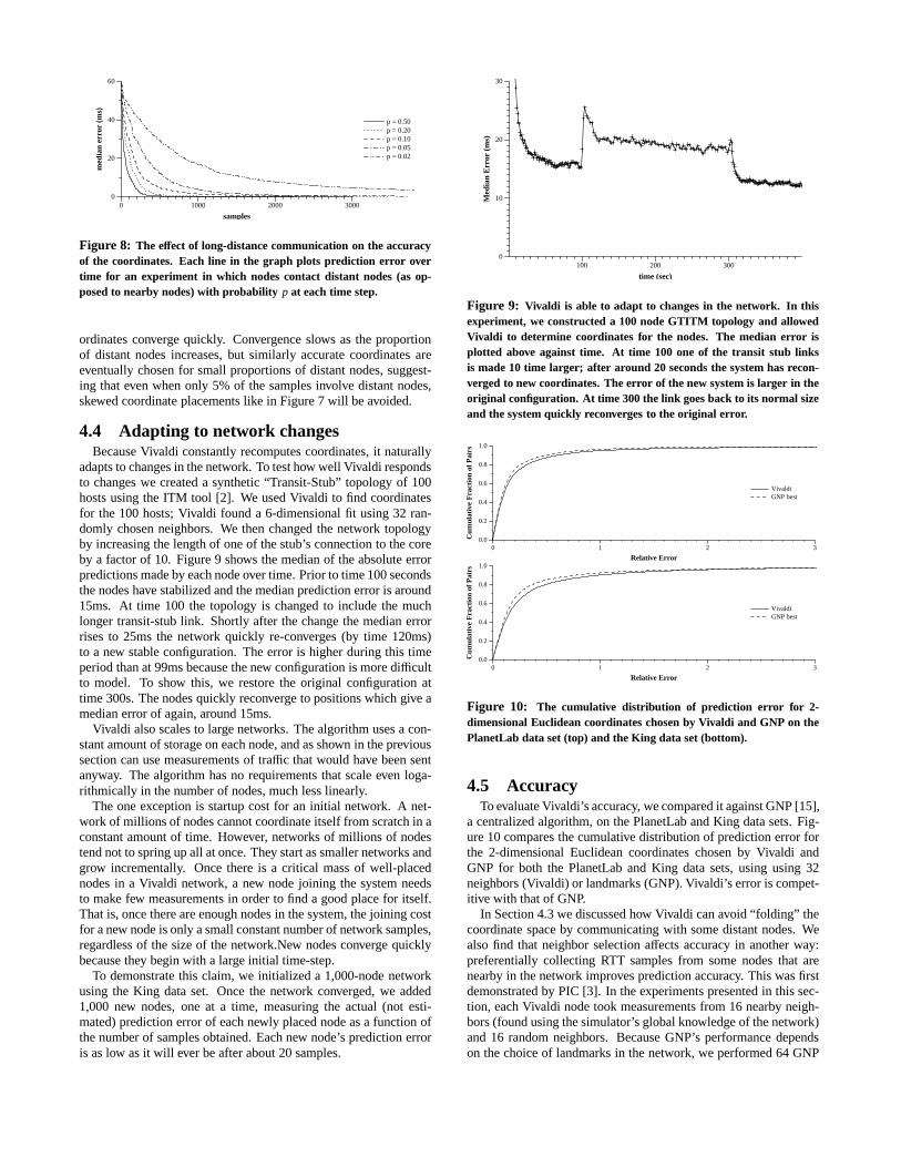
Figure 6: The evolution of a stable 200-node network after 200 new nodes join. When using a constant δ, the new nodes confusethe old nodes, which scatter until the system as a whole has re-converged. In contrast, the adaptive δ (Equation 2) allows new nodesto find their places quickly without disturbing the established order. The graph plots link errors for constant (dotted) and adaptive(solid) δ. At t = 1, the lower line in each pair is the median error among the initial nodes. The higher line in each pair is the medianerror among all pairs. The constant δ system converges more slowly than the adaptive system, disrupting the old nodes significantlyin the process.

convergence; increasing δ to 0.01 causes faster convergence; butincreasing δ again to 1.0 prevents Vivaldi from finding low-errorcoordinates. The reason for the high average error is that the highδ causes the coordinates to oscillate in large steps around the bestvalues.

In Figure 5(b) we repeat the experiment using δ as computed inEquation 2. The data show the effectiveness of using a large δwhena node’s error is high (to converge quickly) and a small δ when anode’s error is low (to minimize the node’s oscillation around goodcoordinates). Empirically, a cc value of 0.25 yields both quick errorreduction and low oscillation.

4.2 Robustness against high-error nodesIdeally, Vivaldi would cope well with large numbers of newly-

joined nodes with inconsistent coordinates. Vivaldi’s adaptive δshould address this problem: when a node joins, it knows its rel-ative error is quite large, and so when it communicates with othernodes, those other nodes will approach it with appropriate skepti-cism.

Figure 6 shows the results of a simulation to test this hypothe-sis. The simulation uses the two-dimensional grid data set to makeit easy to visualize the evolution of the system. The simulationstarted with 200 nodes that already knew coordinates that predictedlatency well. Then we added 200 new nodes to the system and letthe system evolve, using δ = 0.05 in one case and Equation 2 withcc = 0.25 in the other. Figure 6 shows the evolution of the twosystems as well as the error over time. After a few iterations us-ing the constant δ metric, the initial structure of the system hasbeen destroyed, a result of wise old nodes placing too much faith inyoung high-error nodes. Because the initial structure is destroyed,existing nodes can no longer use the current coordinates of otherexisting nodes to predict latency until the system re-converges.

In contrast, the adaptive δ preserves the established order, help-ing the new nodes find their places faster. Also, because the struc-ture of the original nodes is preserved while new nodes join, thosenodes can continue to use current coordinates to make accurate pre-dictions to other original nodes. Finally, the convergence time ofthe new nodes is significantly faster; they converge at t = 60 usingthe relative time-step versus t ≈ 250 using the constant δ.

4.3 Communication patternsAs presented, Vivaldi relies on samples obtained from traffic

generated by the application using it. To understand the range of

Figure 7: A pathological case showing the possible effect ofcommunication patterns on the chosen coordinates. In the firstcase, nodes only contact their four nearest neighbors, allowingthe resulting coordinates to twist over long distances. In thesecond case, nodes contact distant nodes as well, improving theaccuracy of the coordinates at the larger scale.

systems in which this approach is appropriate, we must characterizethe sampling necessary for accurate computation of coordinates.

Some kinds of sampling work badly. For example, Priyanthaet al. [21] show that sampling only nearby (low-latency) nodes canlead to coordinates that preserve local relationships but are far fromcorrect at a global scale. Figure 7 shows the coordinates chosen fornodes laid out in a grid when each node communicates only withits four neighbors. This case is clearly a pathological one, but wewould like to characterize the boundary between normal behaviorand pathology.

The pathological case can be fixed by adding long-distance com-munications, giving the nodes a more global sense of their place inthe network. But how much long-distance communication is nec-essary in order to keep the coordinates from distorting? To answerthis question, we ran an experiment with a grid of 400 nodes. Eachnode was assigned eight neighbors: the four immediately adjacentto it and four chosen at random (on average, the random neighborswill be far away). At each step, each node decides to communicateeither with an adjacent neighbor or a faraway neighbor. Specifi-cally, each node chooses the faraway neighbor set with probabilityp. Then a specific node to sample is chosen from the set at random.

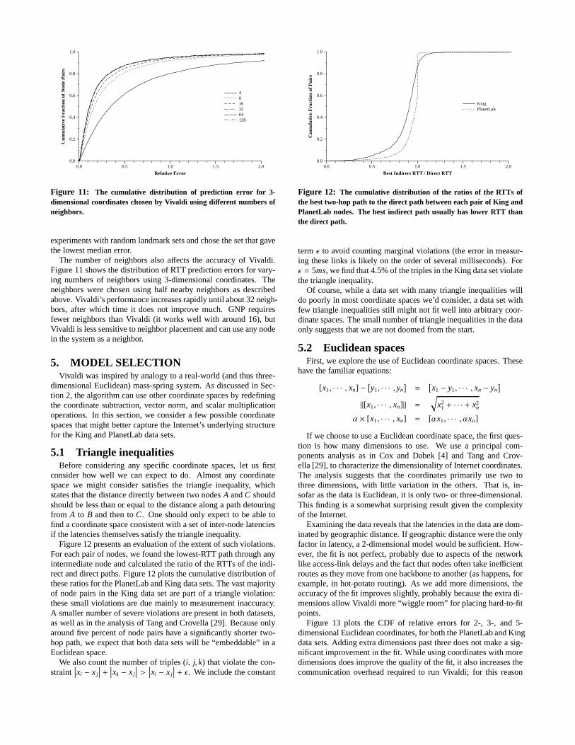
Figure 8 shows the effect of p on the final accuracy of the coor-dinates. When half of the communication is to distant nodes, co-

0 1000 2000 3000

samples

0

20

40

60

med

ian

erro

r (m

s)

p = 0.50p = 0.20p = 0.10p = 0.05p = 0.02

Figure 8: The effect of long-distance communication on the accuracyof the coordinates. Each line in the graph plots prediction error overtime for an experiment in which nodes contact distant nodes (as op-posed to nearby nodes) with probability p at each time step.

ordinates converge quickly. Convergence slows as the proportionof distant nodes increases, but similarly accurate coordinates areeventually chosen for small proportions of distant nodes, suggest-ing that even when only 5% of the samples involve distant nodes,skewed coordinate placements like in Figure 7 will be avoided.

4.4 Adapting to network changesBecause Vivaldi constantly recomputes coordinates, it naturally

adapts to changes in the network. To test how well Vivaldi respondsto changes we created a synthetic “Transit-Stub” topology of 100hosts using the ITM tool [2]. We used Vivaldi to find coordinatesfor the 100 hosts; Vivaldi found a 6-dimensional fit using 32 ran-domly chosen neighbors. We then changed the network topologyby increasing the length of one of the stub’s connection to the coreby a factor of 10. Figure 9 shows the median of the absolute errorpredictions made by each node over time. Prior to time 100 secondsthe nodes have stabilized and the median prediction error is around15ms. At time 100 the topology is changed to include the muchlonger transit-stub link. Shortly after the change the median errorrises to 25ms the network quickly re-converges (by time 120ms)to a new stable configuration. The error is higher during this timeperiod than at 99ms because the new configuration is more difficultto model. To show this, we restore the original configuration attime 300s. The nodes quickly reconverge to positions which give amedian error of again, around 15ms.

Vivaldi also scales to large networks. The algorithm uses a con-stant amount of storage on each node, and as shown in the previoussection can use measurements of traffic that would have been sentanyway. The algorithm has no requirements that scale even loga-rithmically in the number of nodes, much less linearly.

The one exception is startup cost for an initial network. A net-work of millions of nodes cannot coordinate itself from scratch in aconstant amount of time. However, networks of millions of nodestend not to spring up all at once. They start as smaller networks andgrow incrementally. Once there is a critical mass of well-placednodes in a Vivaldi network, a new node joining the system needsto make few measurements in order to find a good place for itself.That is, once there are enough nodes in the system, the joining costfor a new node is only a small constant number of network samples,regardless of the size of the network.New nodes converge quicklybecause they begin with a large initial time-step.

To demonstrate this claim, we initialized a 1,000-node networkusing the King data set. Once the network converged, we added1,000 new nodes, one at a time, measuring the actual (not esti-mated) prediction error of each newly placed node as a function ofthe number of samples obtained. Each new node’s prediction erroris as low as it will ever be after about 20 samples.

100 200 300

time (sec)

0

10

20

30

Med

ian

Err

or (

ms)

Figure 9: Vivaldi is able to adapt to changes in the network. In thisexperiment, we constructed a 100 node GTITM topology and allowedVivaldi to determine coordinates for the nodes. The median error isplotted above against time. At time 100 one of the transit stub linksis made 10 time larger; after around 20 seconds the system has recon-verged to new coordinates. The error of the new system is larger in theoriginal configuration. At time 300 the link goes back to its normal sizeand the system quickly reconverges to the original error.

0 1 2 3

Relative Error

0.0

0.2

0.4

0.6

0.8

1.0

Cum

ulat

ive

Fra

ctio

n of

Pai

rs

VivaldiGNP best

0 1 2 3

Relative Error

0.0

0.2

0.4

0.6

0.8

1.0

Cum

ulat

ive

Fra

ctio

n of

Pai

rs

VivaldiGNP best

Figure 10: The cumulative distribution of prediction error for 2-dimensional Euclidean coordinates chosen by Vivaldi and GNP on thePlanetLab data set (top) and the King data set (bottom).

4.5 AccuracyTo evaluate Vivaldi’s accuracy, we compared it against GNP [15],

a centralized algorithm, on the PlanetLab and King data sets. Fig-ure 10 compares the cumulative distribution of prediction error forthe 2-dimensional Euclidean coordinates chosen by Vivaldi andGNP for both the PlanetLab and King data sets, using using 32neighbors (Vivaldi) or landmarks (GNP). Vivaldi’s error is compet-itive with that of GNP.

In Section 4.3 we discussed how Vivaldi can avoid “folding” thecoordinate space by communicating with some distant nodes. Wealso find that neighbor selection affects accuracy in another way:preferentially collecting RTT samples from some nodes that arenearby in the network improves prediction accuracy. This was firstdemonstrated by PIC [3]. In the experiments presented in this sec-tion, each Vivaldi node took measurements from 16 nearby neigh-bors (found using the simulator’s global knowledge of the network)and 16 random neighbors. Because GNP’s performance dependson the choice of landmarks in the network, we performed 64 GNP

0.0 0.5 1.0 1.5 2.0

Relative Error

0.0

0.2

0.4

0.6

0.8

1.0

Cum

ulat

ive

Fra

ctio

n of

Nod

e P

airs

48163264128

Figure 11: The cumulative distribution of prediction error for 3-dimensional coordinates chosen by Vivaldi using different numbers ofneighbors.

experiments with random landmark sets and chose the set that gavethe lowest median error.

The number of neighbors also affects the accuracy of Vivaldi.Figure 11 shows the distribution of RTT prediction errors for vary-ing numbers of neighbors using 3-dimensional coordinates. Theneighbors were chosen using half nearby neighbors as describedabove. Vivaldi’s performance increases rapidly until about 32 neigh-bors, after which time it does not improve much. GNP requiresfewer neighbors than Vivaldi (it works well with around 16), butVivaldi is less sensitive to neighbor placement and can use any nodein the system as a neighbor.

5. MODEL SELECTIONVivaldi was inspired by analogy to a real-world (and thus three-

dimensional Euclidean) mass-spring system. As discussed in Sec-tion 2, the algorithm can use other coordinate spaces by redefiningthe coordinate subtraction, vector norm, and scalar multiplicationoperations. In this section, we consider a few possible coordinatespaces that might better capture the Internet’s underlying structurefor the King and PlanetLab data sets.

5.1 Triangle inequalitiesBefore considering any specific coordinate spaces, let us first

consider how well we can expect to do. Almost any coordinatespace we might consider satisfies the triangle inequality, whichstates that the distance directly between two nodes A and C shouldshould be less than or equal to the distance along a path detouringfrom A to B and then to C. One should only expect to be able tofind a coordinate space consistent with a set of inter-node latenciesif the latencies themselves satisfy the triangle inequality.

Figure 12 presents an evaluation of the extent of such violations.For each pair of nodes, we found the lowest-RTT path through anyintermediate node and calculated the ratio of the RTTs of the indi-rect and direct paths. Figure 12 plots the cumulative distribution ofthese ratios for the PlanetLab and King data sets. The vast majorityof node pairs in the King data set are part of a triangle violation:these small violations are due mainly to measurement inaccuracy.A smaller number of severe violations are present in both datasets,as well as in the analysis of Tang and Crovella [29]. Because onlyaround five percent of node pairs have a significantly shorter two-hop path, we expect that both data sets will be “embeddable” in aEuclidean space.

We also count the number of triples (i, j, k) that violate the con-straint

∣

∣

∣xi − x j

∣

∣

∣ +∣

∣

∣xk − x j

∣

∣

∣ >∣

∣

∣xi − x j

∣

∣

∣ + ε. We include the constant

0.0 0.5 1.0 1.5 2.0

Best Indirect RTT / Direct RTT

0.0

0.2

0.4

0.6

0.8

1.0

Cum

ulat

ive

Fra

ctio

n of

Pai

rs

KingPlanetLab

Figure 12: The cumulative distribution of the ratios of the RTTs ofthe best two-hop path to the direct path between each pair of King andPlanetLab nodes. The best indirect path usually has lower RTT thanthe direct path.

term ε to avoid counting marginal violations (the error in measur-ing these links is likely on the order of several milliseconds). Forε = 5ms, we find that 4.5% of the triples in the King data set violatethe triangle inequality.

Of course, while a data set with many triangle inequalities willdo poorly in most coordinate spaces we’d consider, a data set withfew triangle inequalities still might not fit well into arbitrary coor-dinate spaces. The small number of triangle inequalities in the dataonly suggests that we are not doomed from the start.

5.2 Euclidean spacesFirst, we explore the use of Euclidean coordinate spaces. These

have the familiar equations:

[x1, · · · , xn] −[

y1, · · · , yn]

=[

x1 − y1, · · · , xn − yn]

‖[x1, · · · , xn]‖ =√

x21 + · · · + x2

n

α × [x1, · · · , xn] = [αx1, · · · , αxn]

If we choose to use a Euclidean coordinate space, the first ques-tion is how many dimensions to use. We use a principal com-ponents analysis as in Cox and Dabek [4] and Tang and Crov-ella [29], to characterize the dimensionality of Internet coordinates.The analysis suggests that the coordinates primarily use two tothree dimensions, with little variation in the others. That is, in-sofar as the data is Euclidean, it is only two- or three-dimensional.This finding is a somewhat surprising result given the complexityof the Internet.

Examining the data reveals that the latencies in the data are dom-inated by geographic distance. If geographic distance were the onlyfactor in latency, a 2-dimensional model would be sufficient. How-ever, the fit is not perfect, probably due to aspects of the networklike access-link delays and the fact that nodes often take inefficientroutes as they move from one backbone to another (as happens, forexample, in hot-potato routing). As we add more dimensions, theaccuracy of the fit improves slightly, probably because the extra di-mensions allow Vivaldi more “wiggle room” for placing hard-to-fitpoints.

Figure 13 plots the CDF of relative errors for 2-, 3-, and 5-dimensional Euclidean coordinates, for both the PlanetLab and Kingdata sets. Adding extra dimensions past three does not make a sig-nificant improvement in the fit. While using coordinates with moredimensions does improve the quality of the fit, it also increases thecommunication overhead required to run Vivaldi; for this reason

0.0 0.5 1.0 1.5 2.0

Relative Error

0.0

0.2

0.4

0.6

0.8

1.0C

umul

ativ

e F

ract

ion

of P

airs

2D3D5D

0.0 0.5 1.0 1.5 2.0

Relative Error

0.0

0.2

0.4

0.6

0.8

1.0

Cum

ulat

ive

Fra

ctio

n of

Pai

rs

2D3D5D

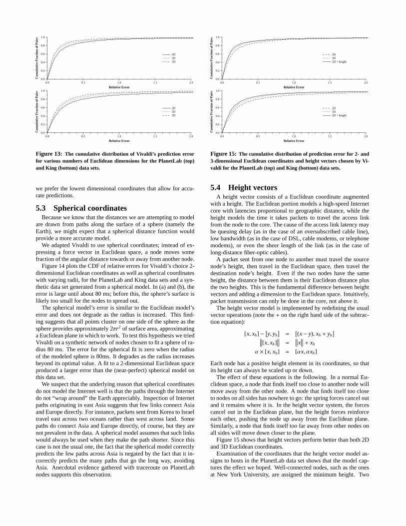
Figure 13: The cumulative distribution of Vivaldi’s prediction errorfor various numbers of Euclidean dimensions for the PlanetLab (top)and King (bottom) data sets.

we prefer the lowest dimensional coordinates that allow for accu-rate predictions.

5.3 Spherical coordinatesBecause we know that the distances we are attempting to model

are drawn from paths along the surface of a sphere (namely theEarth), we might expect that a spherical distance function wouldprovide a more accurate model.

We adapted Vivaldi to use spherical coordinates; instead of ex-pressing a force vector in Euclidean space, a node moves somefraction of the angular distance towards or away from another node.

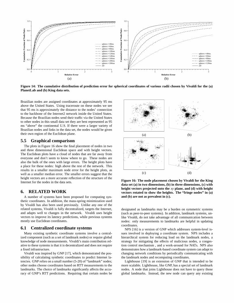
Figure 14 plots the CDF of relative errors for Vivaldi’s choice 2-dimensional Euclidean coordinates as well as spherical coordinateswith varying radii, for the PlanetLab and King data sets and a syn-thetic data set generated from a spherical model. In (a) and (b), theerror is large until about 80 ms; before this, the sphere’s surface islikely too small for the nodes to spread out.

The spherical model’s error is similar to the Euclidean model’serror and does not degrade as the radius is increased. This find-ing suggests that all points cluster on one side of the sphere as thesphere provides approximately 2πr2 of surface area, approximatinga Euclidean plane in which to work. To test this hypothesis we triedVivaldi on a synthetic network of nodes chosen to fit a sphere of ra-dius 80 ms. The error for the spherical fit is zero when the radiusof the modeled sphere is 80ms. It degrades as the radius increasesbeyond its optimal value. A fit to a 2-dimensional Euclidean spaceproduced a larger error than the (near-perfect) spherical model onthis data set.

We suspect that the underlying reason that spherical coordinatesdo not model the Internet well is that the paths through the Internetdo not “wrap around” the Earth appreciably. Inspection of Internetpaths originating in east Asia suggests that few links connect Asiaand Europe directly. For instance, packets sent from Korea to Israeltravel east across two oceans rather than west across land. Somepaths do connect Asia and Europe directly, of course, but they arenot prevalent in the data. A spherical model assumes that such linkswould always be used when they make the path shorter. Since thiscase is not the usual one, the fact that the spherical model correctlypredicts the few paths across Asia is negated by the fact that it in-correctly predicts the many paths that go the long way, avoidingAsia. Anecdotal evidence gathered with traceroute on PlanetLabnodes supports this observation.

0.0 0.5 1.0 1.5 2.0

Relative Error

0.0

0.2

0.4

0.6

0.8

1.0

Cum

ulat

ive

Fra

ctio

n of

Pai

rs

2D3D2D + height

0.0 0.5 1.0 1.5 2.0

Relative Error

0.0

0.2

0.4

0.6

0.8

1.0

Cum

ulat

ive

Fra

ctio

n of

Pai

rs

2D3D2D + height

Figure 15: The cumulative distribution of prediction error for 2- and3-dimensional Euclidean coordinates and height vectors chosen by Vi-valdi for the PlanetLab (top) and King (bottom) data sets.

5.4 Height vectorsA height vector consists of a Euclidean coordinate augmented

with a height. The Euclidean portion models a high-speed Internetcore with latencies proportional to geographic distance, while theheight models the time it takes packets to travel the access linkfrom the node to the core. The cause of the access link latency maybe queuing delay (as in the case of an oversubscribed cable line),low bandwidth (as in the case of DSL, cable modems, or telephonemodems), or even the sheer length of the link (as in the case oflong-distance fiber-optic cables).

A packet sent from one node to another must travel the sourcenode’s height, then travel in the Euclidean space, then travel thedestination node’s height. Even if the two nodes have the sameheight, the distance between them is their Euclidean distance plusthe two heights. This is the fundamental difference between heightvectors and adding a dimension to the Euclidean space. Intuitively,packet transmission can only be done in the core, not above it.

The height vector model is implemented by redefining the usualvector operations (note the + on the right hand side of the subtrac-tion equation):

[x, xh] −[

y, yh]

=[

(x − y), xh + yh]

∥

∥

∥[x, xh]∥

∥

∥ =∥

∥

∥x∥

∥

∥ + xh

α × [x, xh] = [αx, αxh]

Each node has a positive height element in its coordinates, so thatits height can always be scaled up or down.

The effect of these equations is the following. In a normal Eu-clidean space, a node that finds itself too close to another node willmove away from the other node. A node that finds itself too closeto nodes on all sides has nowhere to go: the spring forces cancel outand it remains where it is. In the height vector system, the forcescancel out in the Euclidean plane, but the height forces reinforceeach other, pushing the node up away from the Euclidean plane.Similarly, a node that finds itself too far away from other nodes onall sides will move down closer to the plane.

Figure 15 shows that height vectors perform better than both 2Dand 3D Euclidean coordinates.

Examination of the coordinates that the height vector model as-signs to hosts in the PlanetLab data set shows that the model cap-tures the effect we hoped. Well-connected nodes, such as the onesat New York University, are assigned the minimum height. Two

0 1 2 3

Relative Error

0.0

0.2

0.4

0.6

0.8

1.0

Cum

ulat

ive

Fra

ctio

n of

Nod

e P

airs

sphere r=40mssphere r=60mssphere r=80mssphere r=100mssphere r=120mssphere r=140mssphere r=160mssphere r=200mssphere r=200ms2D

(a)

0 1 2 3

Relative Error

0.0

0.2

0.4

0.6

0.8

1.0

Cum

ulat

ive

Fra

ctio

n of

Nod

e P

airs

sphere r=40mssphere r=60mssphere r=80mssphere r=100mssphere r=120ms2D

(b)

Figure 14: The cumulative distribution of prediction error for spherical coordinates of various radii chosen by Vivaldi for the (a)PlanetLab and (b) King data sets.

Brazilian nodes are assigned coordinates at approximately 95 msabove the United States. Using traceroute on these nodes we seethat 95 ms is approximately the distance to the nodes’ connectionto the backbone of the Internet2 network inside the United States.Because the Brazilian nodes send their traffic via the United Statesto other nodes in this small data set they are best represented as 95ms “above” the continental U.S. If there were a larger variety ofBrazilian nodes and links in the data set, the nodes would be giventheir own region of the Euclidean plane.

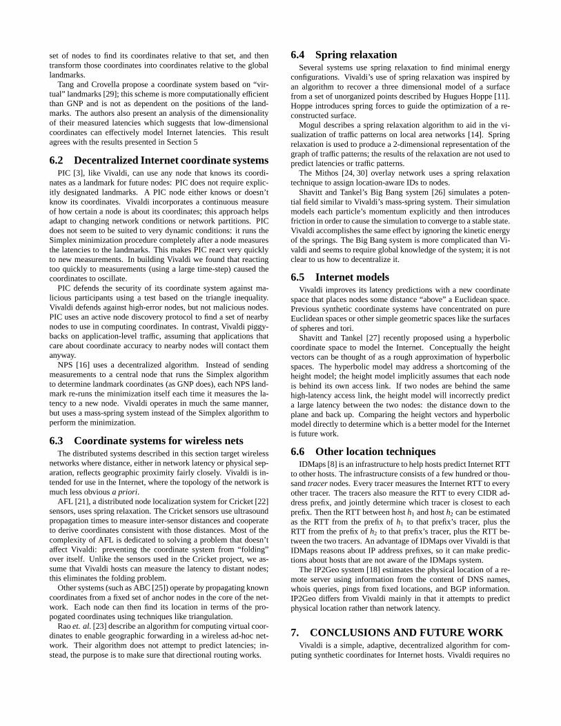
5.5 Graphical comparisonThe plots in Figure 16 show the final placement of nodes in two

and three dimensional Euclidean space and with height vectors.The Euclidean plots have a cloud of nodes that are far away fromeveryone and don’t seem to know where to go. These nodes arealso the bulk of the ones with large errors. The height plots havea place for these nodes: high above the rest of the network. Thisresults in a smaller maximum node error for the height plots, aswell as a smaller median error. The smaller errors suggest that theheight vectors are a more accurate reflection of the structure of theInternet for the nodes in the data sets.

6. RELATED WORKA number of systems have been proposed for computing syn-

thetic coordinates. In addition, the mass-spring minimization usedby Vivaldi has also been used previously. Unlike any one of therelated systems, Vivaldi is fully decentralized, targets the Internet,and adapts well to changes in the network. Vivaldi uses heightvectors to improve its latency predictions, while previous systemsmostly use Euclidean coordinates.

6.1 Centralized coordinate systemsMany existing synthetic coordinate systems involve a central-

ized component (such as a set of landmark nodes) or require globalknowledge of node measurements. Vivaldi’s main contribution rel-ative to these systems is that it is decentralized and does not requirea fixed infrastructure.

Vivaldi was inspired by GNP [17], which demonstrated the pos-sibility of calculating synthetic coordinates to predict Internet la-tencies. GNP relies on a small number (5-20) of “landmark” nodes;other nodes choose coordinates based on RTT measurements to thelandmarks. The choice of landmarks significantly affects the accu-racy of GNP’s RTT predictions. Requiring that certain nodes be

(a) (b)

(c) (d)

Figure 16: The node placement chosen by Vivaldi for the Kingdata set (a) in two dimensions, (b) in three dimensions, (c) withheight vectors projected onto the xy plane, and (d) with heightvectors rotated to show the heights. The “fringe nodes” in (a)and (b) are not as prevalent in (c).

designated as landmarks may be a burden on symmetric systems(such as peer-to-peer systems). In addition, landmark systems, un-like Vivaldi, do not take advantage of all communication betweennodes: only measurements to landmarks are helpful in updatingcoordinates.

NPS [16] is a version of GNP which addresses system-level is-sues involved in deploying a coordinate system. NPS includes ahierarchical system for reducing load on the landmark nodes, astrategy for mitigating the effects of malicious nodes, a conges-tion control mechanism , and a work-around for NATs. NPS alsodemonstrates how a landmark-based coordinate system can adapt tochanging network conditions by periodically communicating withthe landmark nodes and recomputing coordinates.

Lighthouse [19] is an extension of GNP that is intended to bemore scalable. Lighthouse, like GNP, has a special set of landmarknodes. A node that joins Lighthouse does not have to query thoseglobal landmarks. Instead, the new node can query any existing

set of nodes to find its coordinates relative to that set, and thentransform those coordinates into coordinates relative to the globallandmarks.

Tang and Crovella propose a coordinate system based on “vir-tual” landmarks [29]; this scheme is more computationally efficientthan GNP and is not as dependent on the positions of the land-marks. The authors also present an analysis of the dimensionalityof their measured latencies which suggests that low-dimensionalcoordinates can effectively model Internet latencies. This resultagrees with the results presented in Section 5

6.2 Decentralized Internet coordinate systemsPIC [3], like Vivaldi, can use any node that knows its coordi-

nates as a landmark for future nodes: PIC does not require explic-itly designated landmarks. A PIC node either knows or doesn’tknow its coordinates. Vivaldi incorporates a continuous measureof how certain a node is about its coordinates; this approach helpsadapt to changing network conditions or network partitions. PICdoes not seem to be suited to very dynamic conditions: it runs theSimplex minimization procedure completely after a node measuresthe latencies to the landmarks. This makes PIC react very quicklyto new measurements. In building Vivaldi we found that reactingtoo quickly to measurements (using a large time-step) caused thecoordinates to oscillate.

PIC defends the security of its coordinate system against ma-licious participants using a test based on the triangle inequality.Vivaldi defends against high-error nodes, but not malicious nodes.PIC uses an active node discovery protocol to find a set of nearbynodes to use in computing coordinates. In contrast, Vivaldi piggy-backs on application-level traffic, assuming that applications thatcare about coordinate accuracy to nearby nodes will contact themanyway.

NPS [16] uses a decentralized algorithm. Instead of sendingmeasurements to a central node that runs the Simplex algorithmto determine landmark coordinates (as GNP does), each NPS land-mark re-runs the minimization itself each time it measures the la-tency to a new node. Vivaldi operates in much the same manner,but uses a mass-spring system instead of the Simplex algorithm toperform the minimization.

6.3 Coordinate systems for wireless netsThe distributed systems described in this section target wireless

networks where distance, either in network latency or physical sep-aration, reflects geographic proximity fairly closely. Vivaldi is in-tended for use in the Internet, where the topology of the network ismuch less obvious a priori.

AFL [21], a distributed node localization system for Cricket [22]sensors, uses spring relaxation. The Cricket sensors use ultrasoundpropagation times to measure inter-sensor distances and cooperateto derive coordinates consistent with those distances. Most of thecomplexity of AFL is dedicated to solving a problem that doesn’taffect Vivaldi: preventing the coordinate system from “folding”over itself. Unlike the sensors used in the Cricket project, we as-sume that Vivaldi hosts can measure the latency to distant nodes;this eliminates the folding problem.

Other systems (such as ABC [25]) operate by propagating knowncoordinates from a fixed set of anchor nodes in the core of the net-work. Each node can then find its location in terms of the pro-pogated coordinates using techniques like triangulation.

Rao et. al. [23] describe an algorithm for computing virtual coor-dinates to enable geographic forwarding in a wireless ad-hoc net-work. Their algorithm does not attempt to predict latencies; in-stead, the purpose is to make sure that directional routing works.

6.4 Spring relaxationSeveral systems use spring relaxation to find minimal energy

configurations. Vivaldi’s use of spring relaxation was inspired byan algorithm to recover a three dimensional model of a surfacefrom a set of unorganized points described by Hugues Hoppe [11].Hoppe introduces spring forces to guide the optimization of a re-constructed surface.

Mogul describes a spring relaxation algorithm to aid in the vi-sualization of traffic patterns on local area networks [14]. Springrelaxation is used to produce a 2-dimensional representation of thegraph of traffic patterns; the results of the relaxation are not used topredict latencies or traffic patterns.

The Mithos [24, 30] overlay network uses a spring relaxationtechnique to assign location-aware IDs to nodes.

Shavitt and Tankel’s Big Bang system [26] simulates a poten-tial field similar to Vivaldi’s mass-spring system. Their simulationmodels each particle’s momentum explicitly and then introducesfriction in order to cause the simulation to converge to a stable state.Vivaldi accomplishes the same effect by ignoring the kinetic energyof the springs. The Big Bang system is more complicated than Vi-valdi and seems to require global knowledge of the system; it is notclear to us how to decentralize it.

6.5 Internet modelsVivaldi improves its latency predictions with a new coordinate

space that places nodes some distance “above” a Euclidean space.Previous synthetic coordinate systems have concentrated on pureEuclidean spaces or other simple geometric spaces like the surfacesof spheres and tori.

Shavitt and Tankel [27] recently proposed using a hyperboliccoordinate space to model the Internet. Conceptually the heightvectors can be thought of as a rough approximation of hyperbolicspaces. The hyperbolic model may address a shortcoming of theheight model; the height model implicitly assumes that each nodeis behind its own access link. If two nodes are behind the samehigh-latency access link, the height model will incorrectly predicta large latency between the two nodes: the distance down to theplane and back up. Comparing the height vectors and hyperbolicmodel directly to determine which is a better model for the Internetis future work.

6.6 Other location techniquesIDMaps [8] is an infrastructure to help hosts predict Internet RTT

to other hosts. The infrastructure consists of a few hundred or thou-sand tracer nodes. Every tracer measures the Internet RTT to everyother tracer. The tracers also measure the RTT to every CIDR ad-dress prefix, and jointly determine which tracer is closest to eachprefix. Then the RTT between host h1 and host h2 can be estimatedas the RTT from the prefix of h1 to that prefix’s tracer, plus theRTT from the prefix of h2 to that prefix’s tracer, plus the RTT be-tween the two tracers. An advantage of IDMaps over Vivaldi is thatIDMaps reasons about IP address prefixes, so it can make predic-tions about hosts that are not aware of the IDMaps system.

The IP2Geo system [18] estimates the physical location of a re-mote server using information from the content of DNS names,whois queries, pings from fixed locations, and BGP information.IP2Geo differs from Vivaldi mainly in that it attempts to predictphysical location rather than network latency.

7. CONCLUSIONS AND FUTURE WORKVivaldi is a simple, adaptive, decentralized algorithm for com-

puting synthetic coordinates for Internet hosts. Vivaldi requires no

fixed infrastructure, supports a wide range of communication pat-terns, and is able to piggy-back network sampling on applicationtraffic. Vivaldi includes refinements that adaptively tune its timestep parameter to cause the system to converge to accurate solu-tions quickly and to maintain accuracy even as large numbers ofnew hosts join the network.

By evaluating the performance of Vivaldi on a large data set gen-erated from measurements of Internet hosts, we have investigatedthe extent to which the Internet can be represented in simple ge-ometric spaces. We propose a new model, height vectors, whichshould be of use to all coordinate algorithms. Attempting to un-derstand characteristics of the Internet by studying the way it ismodeled by various geometric spaces is a promising line of futureresearch.

Because Vivaldi requires no infrastructure and is simple to im-plement, it is easy to deploy in existing applications. We modifiedDHash, a distributed hash table, to take advantage of Vivaldi andreduced time required to fetch a block in DHash by 40% on a globaltest-bed [7]. We hope that Vivaldi’s simplicity will allow other dis-tributed systems to adopt it.

AcknowledgmentsThis research was conducted as part of the IRIS project(http://project-iris.net/), supported by the National Sci-ence Foundation under Cooperative Agreement No. ANI-0225660.Russ Cox is supported by a fellowship from the Fannie and JohnHertz Foundation.

REFERENCES[1] BitTorrent. http://bitconjurer.org/BitTorrent/protocol.html.[2] K. L. Calvert, M. B. Doar, and E. W. Zegura. Modeling

Internet topology. IEEE Communications, 35(6):160–163,June 1997.

[3] M. Costa, M. Castro, A. Rowstron, and P. Key. PIC: PracticalInternet coordinates for distance estimation. In InternationalConference on Distributed Systems, Tokyo, Japan, March2004.

[4] R. Cox and F. Dabek. Learning Euclidean coordinates forInternet hosts. http://pdos.lcs.mit.edu/˜rsc/6867.pdf,December 2002.

[5] R. Cox, F. Dabek, F. Kaashoek, J. Li, and R. Morris.Practical, distributed network coordinates. In Proceedings ofthe Second Workshop on Hot Topics in Networks(HotNets-II), Cambridge, Massachusetts, November 2003.

[6] F. Dabek, M. F. Kaashoek, D. Karger, R. Morris, andI. Stoica. Wide-area cooperative storage with CFS. In Proc.18th ACM Symposium on Operating Systems Principles(SOSP ’01), pages 202–205, Oct. 2001.

[7] F. Dabek, J. Li, E. Sit, J. Robertson, M. F. Kaashoek, andR. Morris. Designing a DHT for low latency and highthroughput. In Proceedings of the 1st USENIX Symposiumon Networked Systems Design and Implementation (NSDI’04), San Francisco, California, March 2004.

[8] P. Francis, S. Jamin, C. Jin, Y. Jin, D. Raz, Y. Shavitt, andL. Zhang. IDMaps: A global Internet host distanceestimation service. IEEE/ACM Transactions on Networking,Oct. 2001.

[9] T. Gil, J. Li, F. Kaashoek, and R. Morris. Peer-to-peersimulator, 2003. http://pdos.lcs.mit.edu/p2psim.

[10] K. P. Gummadi, S. Saroiu, and S. D. Gribble. King:Estimating latency between arbitrary Internet end hosts. In

Proc. of SIGCOMM IMW 2002, pages 5–18, November2002.

[11] H. Hoppe. Surface reconstruction from unorganized points.PhD thesis, Department of Computer Science andEngineering, University of Washington, 1994.

[12] KaZaA media dekstop. http://www.kazaa.com/.[13] P. Mockapetris and K. J. Dunlap. Development of the

Domain Name System. In Proc. ACM SIGCOMM, pages123–133, Stanford, CA, 1988.

[14] J. C. Mogul. Efficient use of workstations for passivemonitoring of local area networks. Research Report 90/5,Digital Western Research Laboratory, July 1990.

[15] E. Ng. GNP software, 2003. http://www-2.cs.cmu.edu/˜eugeneng/research/gnp/software.html.

[16] T. E. Ng and H. Zhang. A network positioning system for theInternet. In Proc. USENIX Conference, June 2004.

[17] T. S. E. Ng and H. Zhang. Predicting Internet networkdistance with coordinates-based approaches. In Proceedingsof IEEE Infocom, pages 170–179, 2002.

[18] V. Padmanabhan and L. Subramanian. An investigation ofgeographic mapping techniques for Internet hosts. In Proc.ACM SIGCOMM, pages 173–185, San Diego, Aug. 2001.

[19] M. Pias, J. Crowcroft, S. Wilbur, T. Harris, and S. Bhatti.Lighthouses for scalable distributed location. In IPTPS,2003.

[20] Planetlab. www.planet-lab.org.[21] N. Priyantha, H. Balakrishnan, E. Demaine, and S. Teller.

Anchor-free distributed localization in sensor networks.Technical Report TR-892, MIT LCS, Apr. 2003.

[22] N. Priyantha, A. Chakraborty, and H. Balakrishnan. TheCricket Location-Support System. In Proc. 6th ACMMOBICOM Conf., Boston, MA, Aug. 2000.

[23] A. Rao, S. Ratnasamy, C. Papadimitriou, S. Shenker, andI. Stoica. Geographic routing without location information.In ACM MobiCom Conference, pages 96 – 108, Sept. 2003.

[24] R. Rinaldi and M. Waldvogel. Routing and data location inoverlay peer-to-peer networks. Research Report RZ–3433,IBM, July 2002.

[25] C. Savarese, J. M. Rabaey, and J. Beutel. Locationing indistributed ad-hoc wireless sensor networks. In ICASSP,pages 2037–2040, May 2001.

[26] Y. Shavitt and T. Tankel. Big-bang simulation for embeddingnetwork distances in Euclidean space. In Proc. of IEEEInfocom, April 2003.

[27] Y. Shavitt and T. Tankel. On the curvature of the Internet andits usage for overlay construction and distance estimation. InProc. of IEEE Infocom, April 2004.

[28] J. Stribling. All-pairs-ping trace of PlanetLab, 2004.http://pdos.lcs.mit.edu/ strib/.

[29] L. Tang and M. Crovella. Virtual landmarks for the Internet.In Internet Measurement Conference, pages 143 – 152,Miami Beach, FL, October 2003.

[30] M. Waldvogel and R. Rinaldi. Efficient topology-awareoverlay network. In Hotnets-I, 2002.

[31] L. Wang, V. Pai, and L. Peterson. The Effectiveness ofRequest Redirecion on CDN Robustness. In Proceedings ofthe Fifth Symposium on Operating Systems Design andImplementation, Boston, MA USA, December 2002.