vision based robust vehicle detection...
TRANSCRIPT
VISION BASED ROBUST VEHICLE DETECTION AND TRACKING VIA ACTIVELEARNING
By
VISHNU KARAKKAT NARAYANAN
A THESIS PRESENTED TO THE GRADUATE SCHOOLOF THE UNIVERSITY OF FLORIDA IN PARTIAL FULFILLMENT
OF THE REQUIREMENTS FOR THE DEGREE OFMASTER OF SCIENCE
UNIVERSITY OF FLORIDA
2013

c⃝ 2013 Vishnu Karakkat Narayanan
2

To my parents, P.V. Narayanan and Sudha Narayanan
3

ACKNOWLEDGMENTS
I would like to express my gratitude to my adviser Dr. Carl Crane for his contribution
and guidance during the project phase and throughout my Masters study. I would also
like to thank my committee members Dr. Prabir Barooah and Dr. Antonio Arroyo for their
help and suggestions.
Furthermore, I am extremely grateful to my lab members Ryan Chilton, Maninder
Singh Panda and Darshan Patel for their assistance. I would like to extend a big thank
you to Clint P. George for his help in writing this thesis. I offer my regards to all my
friends who directly or indirectly contributed towards building this system especially Paul
Thotakkara, Rahul Subramany, Gokul Bhat and Jacob James.
Finally, I thank my parents Sudha Narayanan and P.V. Narayanan and my brother
Varun Narayanan for all their encouragement, everlasting love and care which was the
guiding light throughout my studies and my life and without whom I would never be in
this position.
4

TABLE OF CONTENTS
page
ACKNOWLEDGMENTS . . . . . . . . . . . . . . . . . . . . . . . . . . . . . . . . . . 4
LIST OF TABLES . . . . . . . . . . . . . . . . . . . . . . . . . . . . . . . . . . . . . . 7
LIST OF FIGURES . . . . . . . . . . . . . . . . . . . . . . . . . . . . . . . . . . . . . 8
ABSTRACT . . . . . . . . . . . . . . . . . . . . . . . . . . . . . . . . . . . . . . . . . 9
CHAPTER
1 INTRODUCTION . . . . . . . . . . . . . . . . . . . . . . . . . . . . . . . . . . . 10
1.1 Organization . . . . . . . . . . . . . . . . . . . . . . . . . . . . . . . . . . 12
2 RELATED RESEARCH . . . . . . . . . . . . . . . . . . . . . . . . . . . . . . . 13
2.1 Vision Based Vehicle Detection . . . . . . . . . . . . . . . . . . . . . . . . 132.1.1 Machine Learning Based Approaches . . . . . . . . . . . . . . . . 152.1.2 Active Learning Based Object Classification . . . . . . . . . . . . . 17
2.2 Vehicle Tracking And Distance Estimation . . . . . . . . . . . . . . . . . . 192.2.1 Vehicle Tracking . . . . . . . . . . . . . . . . . . . . . . . . . . . . . 192.2.2 Distance Estimation From a Monocular Camera . . . . . . . . . . . 21
2.3 Summary . . . . . . . . . . . . . . . . . . . . . . . . . . . . . . . . . . . . 22
3 ACTIVELY TRAINED VIOLA-JONES CLASSIFIER . . . . . . . . . . . . . . . . 23
3.1 Viola-Jones Object Detection Framework . . . . . . . . . . . . . . . . . . 233.1.1 Feature Selection and Image Representation . . . . . . . . . . . . 23
3.1.1.1 Rectangular Haar-like features . . . . . . . . . . . . . . . 233.1.1.2 Integral image representation . . . . . . . . . . . . . . . . 24
3.1.2 Adaboost Based Classifier . . . . . . . . . . . . . . . . . . . . . . . 253.1.3 Classifier Cascade . . . . . . . . . . . . . . . . . . . . . . . . . . . 27
3.2 Passively Trained Classifier . . . . . . . . . . . . . . . . . . . . . . . . . . 283.3 Active Learning Principles . . . . . . . . . . . . . . . . . . . . . . . . . . . 30
3.3.1 Query By Confidence . . . . . . . . . . . . . . . . . . . . . . . . . 313.3.2 Query By Misclassification . . . . . . . . . . . . . . . . . . . . . . . 31
3.4 Active Learning Based Classifier . . . . . . . . . . . . . . . . . . . . . . . 323.5 Summary . . . . . . . . . . . . . . . . . . . . . . . . . . . . . . . . . . . . 34
4 VEHICLE TRACKING AND DISTANCE ESTIMATION . . . . . . . . . . . . . . 35
4.1 Lucas-Kanade Optical Flow Based Tracking . . . . . . . . . . . . . . . . . 354.1.1 Method . . . . . . . . . . . . . . . . . . . . . . . . . . . . . . . . . 364.1.2 Pyramidal Implementation . . . . . . . . . . . . . . . . . . . . . . . 374.1.3 Implementation . . . . . . . . . . . . . . . . . . . . . . . . . . . . . 38
4.2 Distance Estimation . . . . . . . . . . . . . . . . . . . . . . . . . . . . . . 39
5

4.3 Summary . . . . . . . . . . . . . . . . . . . . . . . . . . . . . . . . . . . . 41
5 EVALUATION AND DISCUSSION . . . . . . . . . . . . . . . . . . . . . . . . . 43
5.1 Datasets . . . . . . . . . . . . . . . . . . . . . . . . . . . . . . . . . . . . . 435.1.1 Caltech 2001/1999 Static Image Database . . . . . . . . . . . . . . 435.1.2 mvBlueFOX Test Data . . . . . . . . . . . . . . . . . . . . . . . . . 43
5.2 Evaluation Parameters . . . . . . . . . . . . . . . . . . . . . . . . . . . . . 455.3 Static Dataset . . . . . . . . . . . . . . . . . . . . . . . . . . . . . . . . . . 465.4 Real Time Dataset . . . . . . . . . . . . . . . . . . . . . . . . . . . . . . . 495.5 Implementation in a Real Time Scenario . . . . . . . . . . . . . . . . . . . 535.6 Summary . . . . . . . . . . . . . . . . . . . . . . . . . . . . . . . . . . . . 53
6 CONCLUSIONS AND FUTURE WORK . . . . . . . . . . . . . . . . . . . . . . 55
REFERENCES . . . . . . . . . . . . . . . . . . . . . . . . . . . . . . . . . . . . . . . 57
BIOGRAPHICAL SKETCH . . . . . . . . . . . . . . . . . . . . . . . . . . . . . . . . 62
6

LIST OF TABLES
Table page
3-1 Passive Training Parameters . . . . . . . . . . . . . . . . . . . . . . . . . . . . 30
3-2 Active Training Parameters . . . . . . . . . . . . . . . . . . . . . . . . . . . . . 34
5-1 Results on Static Dataset - Active-Passive Comparision . . . . . . . . . . . . . 47
5-2 Results on Real Time Dataset - Active-Passive Comparision . . . . . . . . . . 52
7

LIST OF FIGURES
Figure page
3-1 Rectangular Haar-like Features . . . . . . . . . . . . . . . . . . . . . . . . . . . 24
3-2 Integral Image Representation . . . . . . . . . . . . . . . . . . . . . . . . . . . 26
3-3 Schematic of a Classifier Cascade . . . . . . . . . . . . . . . . . . . . . . . . . 27
3-4 Example of a positive image . . . . . . . . . . . . . . . . . . . . . . . . . . . . . 29
3-5 Example of a negative image . . . . . . . . . . . . . . . . . . . . . . . . . . . . 30
3-6 Schematic of the Active Learning Framework . . . . . . . . . . . . . . . . . . . 33
3-7 Examples queried for re-training . . . . . . . . . . . . . . . . . . . . . . . . . . 33
4-1 Pyramidal Implementation of LK Optical Flow . . . . . . . . . . . . . . . . . . . 38
4-2 Schematic showing the algorithmic flow of the Tracking Process . . . . . . . . 39
4-3 Algorithmic flow of the complete Detection and Tracking Process . . . . . . . . 42
5-1 Caltech 2001/1999 Static Image Data Example . . . . . . . . . . . . . . . . . . 44
5-2 Real Time test data captured using the test rig . . . . . . . . . . . . . . . . . . 44
5-3 Examples of True Positive Detections in Static Datset . . . . . . . . . . . . . . 47
5-4 Examples of false positives and missed detections . . . . . . . . . . . . . . . . 47
5-5 The ROC curves for Actively and Passively Trained Classifiers . . . . . . . . . 48
5-6 Examples of True Positive Detections in Real Time Test set . . . . . . . . . . . 49
5-7 Examples of false positives and missed detections . . . . . . . . . . . . . . . . 50
5-8 Test data Detection Track . . . . . . . . . . . . . . . . . . . . . . . . . . . . . . 50
5-9 The ROC curves for Actively and Passively Trained Classifiers . . . . . . . . . 52
5-10 Screenshot of Full System 1 . . . . . . . . . . . . . . . . . . . . . . . . . . . . 53
5-11 Screenshot of Full System 2 . . . . . . . . . . . . . . . . . . . . . . . . . . . . 54
8

Abstract of Thesis Presented to the Graduate Schoolof the University of Florida in Partial Fulfillment of the
Requirements for the Degree of Master of Science
VISION BASED ROBUST VEHICLE DETECTION AND TRACKING VIA ACTIVELEARNING
By
Vishnu Karakkat Narayanan
May 2013
Chair: Carl D.Crane, IIIMajor: Mechanical Engineering
This thesis aims to introduce a novel robust real time system capable of rapidly
detecting and tracking vehicles in a video stream using a monocular vision system. The
framework used for this purpose is an actively learned implementation of the Haar-like
feature based Viola-Jones classifier integrated with a Lucas-Kanade Optical Flow
Tracker and a distance estimation algorithm.
A passively trained supervised system is initially built by using Rectangular
Haar-like features. Several increasingly complex weak classifiers,(which are essentially
a degenerative set of Decision Tree classifiers) are trained at the start. These weakly
trained classifiers are then conjunctively cascaded based on Adaboost to form a strong
classifier which results in the elimination of much of the background and works on
regions of the image which are more likely to be the candidate. This leads to an
increase in speed and reduction in false alarm rates.
An actively learned model is then generated from the initial passive classifier by
querying misclassified instances when the model is evaluated on an independent
dataset. This actively trained system is then integrated with a Lucas-Kanade optical flow
tracker and distance estimator algorithm to build a complete multi-vehicle detection and
tracking system capable of performing in real time. The built model is then evaluated
extensively on static as well as real world data and results are presented.
9

CHAPTER 1INTRODUCTION
More people are affected by automotive accident injuries than any other accident
related injuries. It has been estimated that every year, about 20 - 50 million people are
injured due to automotive accidents. Around 1.2 million people lose their lives as a
result. There are reports suggesting that 1 to 3% of the world’s domestic gross product
is spent on health care and other costs which are attributed to auto accidents.
Consequently, over the last decade, there has been a lot of research purely devoted to
the study and development of intelligent automotive safety systems and safe
autonomous vehicles among the Intelligent Transportation and Robotics community.
A majority of such research conducted by academicians and vehicle manufacturers
in this field is related to the development of systems which are capable of detecting and
tracking other vehicles in real time traffic by using a variety of sensors like cameras,
LiDaRs (Laser Detection and Ranging Sensor) and infrared sensors. One of the main
challenges associated with developing such systems is that they should be reliable,
robust and simple to implement [28]. Currently, the majority of such systems employ
LiDaR based sensing which provide highly accurate information but does not posses a
mechanism which can be exploited for enhanced and intuitive decision making. Vision
based vehicle detection systems have been widely credited and researched as the one
that is low cost, efficient, and has the potential to deliver accurate information to the
driver regarding traffic, pedestrians, lane following and lane departures.
The purpose of this thesis is to shed some light on the application of machine
learning techniques in the area of robust, real time vehicle detection based on vision. It
is a well-known fact that vision based vehicle detection is a challenging problem, as the
environment is ever changing, dynamic, and cluttered. The vehicles are constantly in
motion, there exists a diverse array of vehicle sizes and shapes, and illumination is not
constant. So, a general pattern recognition based model for designing such a system
10

would be of little value. Therefore, this thesis makes the use of an ”actively trained”
cascade of boosted classifiers which are trained on a real time dataset to efficiently
detect vehicles in motion. The underlying framework, initially developed for face
detection by Viola and Jones [14], is particularly useful for the application at hand
because it eliminates the effects of occlusion, scale invariance and shape constraints
which are inherent in cluttered scenes like the traffic stream.
Active Learning is an upcoming field of research in Machine Learning circles. The
principle of active learning is the notion that a classifier (or learning function) has the
ability to have some degree of control over the data which it learns. This theory has
been successfully implemented in areas like document modeling, text categorization,
and natural language processing with significant improvements in classification accuracy
and computational load. This study aims to use active learning to tweak the classifier
built using the Viola-Jones framework mainly to reduce the occurrence of false positives
in on-road detection along with improvement in accuracy.
The actively trained system is then integrated with a tracking algorithm based on
Lucas-Kanade Optical Flow and a vehicle range estimation algorithm to build a complete
multi-vehicle detection and tracking system based on monocular vision which is reliable,
robust and capable of performing in real time using standard hardware. An exhaustive
performance analysis is also presented by evaluating the designed system in static as
well as real world datasets. A comparison between the passively trained and the actively
trained classifier is also explained and some avenues for future work are explored.
The major contribution of the thesis is a preliminary investigation into active learning
based real time vehicle detection in traffic using a monocular vision system. Evaluations
on real time and static image datasets sheds light on the systems recall, localization and
robustness.
11

1.1 Organization
The thesis is organized as follows:
Chapter 2 provides a comprehensive study on the research pertaining to the current
study explaining the evolution of vision based vehicle detection, the development of
machine learning based vision processing and active learning based on road vehicle
detection. Background regarding vision based tracking and 3-D range estimation is also
given. Chapter 3 initially discusses the Viola-Jones framework along with design of a
passive classifier trained on real world data. The chapter then moves to discuss Active
Learning principles and explains the construction of an Actively trained classifier by
improving upon the passive classifier. Chapter 4 delineates the Lucas-Kanade Feature
tracking employed in this work in conjunction with the active classifier. A distance
estimation method based on a pin-hole camera model is also explained. Further,
Chapter 5 contains evaluations and discussions regarding the implementation of the
multi-vehicle detection and tracking system on real world and static datasets. An
exhaustive performance analysis is presented along with scope for improvement. Finally,
Chapter 6 summarizes the whole idea of the thesis and discusses the direction of future
work.
12

CHAPTER 2RELATED RESEARCH
An exhaustive overview of the research in the field of vision based vehicle detection
and tracking is presented in this chapter. The literature pertaining to this work can be
broadly divided into two categories. The first part deals with papers concerning vehicle
detection based on vision. Starting from the algorithmic approach to the machine
learning approach, the beautiful hierarchy of the evolution and improvements in this area
is presented. The second part explains and critiques papers concerned with vehicle
tracking along with works relative to distance estimation from a single camera. Finally, a
summary of all the techniques is presented, along with the brief introduction of the novel
improvements that this present work aims to introduce.
2.1 Vision Based Vehicle Detection
Vehicle detection based on vision has had tremendous research exposure in the
past two decades, both from the Artificial Intelligence and Robotics community and the
Intelligent Transportation Systems community (wherein, the majority of research is on
vision based systems for vehicle detection). Therefore, a plethora of work relevant to this
area can be found which are evaluated both on real-time and static images.
The transition from stereo vision to monocular vision in the case of vehicle detection
can be best explained from the work of Bensrhair et al. [2]. The work presents a
co-operative approach to vehicle detection, where monocular vision based and stereo
vision based systems are evaluated individually and in an integrated system. The
monocular system used a simple model based template matching for the detection
purpose. The study found out that stereo systems were 10 times slower than monocular
systems when evaluated on static images but had higher accuracy in detecting and
estimating the actual distance. A similar system was developed recently by Sivaraman
[27]. This system used an actively trained monocular system (based on Haar-like
13

features) along with a stereo rig to calculate the depth map. The system had very high
accuracy but took 50ms to process a single frame.
Betke et al. [3], utilized the combination of edge, color, and motion information to
detect possible vehicles and lane markings. This was one of the earliest and possibly
one of the most defining attempts at performing real-time vision based vehicle detection
and tracking. The algorithm used a combination of template matching and a temporal
differencing method performed on online cropped images to detect cars. Lane markings
and track boundaries were tracked using a recursive least squares filter. The final
system was capable of performing at around 15 frames/sec in real-time but had
moderate accuracy. The amount of time required for pre-processing and algorithm
development does not justify the use of this method in the present scenario.
A different approach was introduced by Yamaguchi et al. [34] where the ego-motion
of the vehicle (the motion of the vehicle camera) was estimated to initially construct a
3-D representation of the scene and then detect a vehicle. The ego-motion is estimated
by the correspondence of some feature points between two different images in which the
objects are not moving. After the 3-D reconstruction process, vehicles are detected by
triangulation. This system was capable of performing at 10 frames/sec but again
suffered from a high false positive rate.
Vehicle detection at nighttime is also an open avenue for research. The above
mentioned techniques cannot be used successfully in a nighttime scenario. Chen et al.
[7] proposed a pattern analysis based on a tail light clustering approach for vehicle
classification. This system (which can be only employed at night) was able to detect cars
as well as motorbikes with an accuracy of 97.5%.
Detecting vehicles in traffic from an overhead camera mounted inside a tunnel was
explored by Wu et al [33]. The proposed algorithm constructed an automatic lane
detection system by background subtraction and detected vehicles using a block
matching technique. This method is suitable for overhead traffic detection but it cannot
14

be scaled to rear end systems where the camera is moving constantly and the scene
changes at every frame. Thus, methods based on static block matching or template
matching are not suitable for the present scenario.
Although Image Processing techniques provide a sound theoretical framework for
on-road vehicle detection, the moderate accuracy and high implementation time has
deviated this research towards machine learning techniques to solve this problem.
2.1.1 Machine Learning Based Approaches
One of the more important aspects of Machine Learning is the selection of suitable
features for classification [22]. Selecting features in cluttered scenes like traffic streams
for object detection is not a trivial issue. The majority of work reported in this area uses
either Histogram of Gradient (HOG) features or Haar-like features coupled with a
suitable learning algorithm for object classification.
Balcones et al. [1] proposed a rear end collision warning system which used an
extensively pre-processed image sequence trained on HOG features and classified
using a Support Vector Machine (SVM). The detected Region of Interest (ROI) was
tracked using a Kalman filter. This system achieved very high detection rates but
suffered from a very high false positive rate also.
A similar system was derived by Sun et al. [21] where the features were selected
based on Haar wavelet transforms instead of HOG features. An SVM based classifier
was used to verify the hypotheses generated by the feature detection algorithm. This
system gave a frame rate of 10 Hz when implemented in real time. But the accuracy was
found to be moderate with high false positive rates.
A pioneering work in the area of Machine Learning based object detection was
reported by Papageorgiou [24] in the year 2000. The paper proposed a binary Support
Vector Machine (SVM) based classifier trained on Haar wavlet transforms, which are
essentially the intensity differences between different regions of an image. This method
15

was tailor made for object detection in cluttered scenes. Results were presented on
static images for pedestrian detection, face detection, and car detection.
In 2001, Micheal Jones and Paul Viola [14] presented their work on Robust object
detection through training Haar-like features via Adaboost. This was in effect a major
improvement from the algorithm proposed by Papageorgiou as the system allowed very
rapid detection which facilitated the use of the algorithm in real time systems. This
theory was validated by employing the algorithm for the purpose of face detection with
highly satisfactory results. An implementation of this very framework is used in this
thesis and is explained in detail in the following chapter. Much of the later work in the
area of vision based vehicle detection uses a derivative of this framework.
The Viola-Jones algorithm thus has become a very popular framework for
monocular vision based object detection. Han et al. [12] derived a simplistic approach to
the implementation of this framework to vehicle detection systems. This algorithm
searches the image for objects with shadow and eliminates the rest of the image region
as noise removal. Then the Haar-like feature detector is run on the image to classify the
ROI as a vehicle or non-vehicle. This study used static images of cars for training
purposes, thus the accuracy of the classifier was limited to around 82% average.
A real time system based on Haar-like features combined with Pairwise Geometrical
Histograms (PGH) was proposed by Yong et al [35]. PGH is a powerful shape descriptor
which is invariant to rotation. The study compared the accuracy of classifiers built with
Haar-like features and the combination of Haar-like features and PGH. The results
showed that the combination classifier performed at 95.2% accuracy when compared to
92.4% for the single type feature classifier. The false positive rate was relatively the
same.
A different method was proposed by Khalid et al [16] wherein a hypothesis was
initially generated by a corner detector algorithm and this hypothesis was verified by
running the generated ROI through an Adaboost based classifer. The classifier was
16

trained on static images, but the system gave good accuracy as a lot of false positive
candidates were eliminated during the corner and edge detection process. But the lack
of a good tracking algorithm hinders the implementation of this system in real world
applications.
Choi [8] integrated an oncoming traffic detector based on ’optical flow’ along with
the traditional rear traffic detector to construct a comprehensive vehicle detection
algorithm. The optical flow was based on correspondence of features detected by the
Shi-Tomasi corner detector. The rear end vehicle detection system was also based on
Adaboost working with Haar-like features. Again, the classifier was trained using generic
static images of cars and were validated on static images with an accuracy of 89%. A
Kalman filter was integrated with the system for tracking previously detected vehicles.
An exhaustive study was conducted by Tsai et al. [32] in which a fully real time
compatible system was developed for vehicle detection. The framework initially
generates a hypothesis based on a corner detector with SURF based descriptors and
validates the hypothesis based on the Viola-Jones algorithm. A Kalman filer based
tracker was integrated to the system. The study also compared the classification
accuracy with respect to the actual distance of the vehicle from the ego-vehicle. The
minimum accuracy achieved was 91.2% with a threshold maximum distance of 140m.
2.1.2 Active Learning Based Object Classification
Active Learning (AL), in brief, is a system which is able to ask a user (or some other
information source) interactively about the output of some data point. It is fully explained
in the next chapter with conclusive examples and theory. This chapter just focuses on
the background of work done in this area. AL is being increasingly used in conjunction
with object detection among the Robotics research circle. Among the many advantages
are improvement of classifier performance, reduction of false alarm rates and generation
of new data for training. These are the major factors that validates active learning as a
valuable tool for machine learning based object detection. One of the major drawbacks
17

of the Viola-Jones algorithm is the issue of high false alarm rates. Thus, the use of
active learning together with the Viola-Jones algorithm could lead to a robust classifier.
An entropy based approach for object detection based on Active Learning was
proposed by Holub [13]. The study focused on reduction in the amount of training
samples required by interactively selecting the images which had higher and better
feature density. This was achieved by querying some sort of maximized information
about each image. The study achieved up to 10x reductions in the number of training
samples among the 170 categories of images analyzed.
The backbone of Active Learning is the the selection of samples for interactive
labeling of an evaluated dataset. Kapoor et al [15] devised a system based on Gaussian
Processes with co-variance functions based on Pyramid Matching Kernels for
autonomously and optimally selecting data for interactive labeling. This reduces the time
consumed by the vision researcher in labeling the dataset. The major advantage of this
system is that it can be employed in very large datasets with a small tradeoff in the
classification accuracy.
Much of the literature in the field of using Active Learning for specifically vehicle
detection owes to the work of Sivaraman [30] [29]. In two different papers, the author
compared two different methods of generating training samples, i.e. Query by sampling
and Query by misclassification. The results showed that even though Query by
misclassification was subject to higher human capital, it lead to better accuracy. The
accuracy achieved was 95% with a false positive rate of 6.4%. This proved a significant
reduction in false positives when compared to the passive learning methods mentioned
above. The study also integrated a Condensation filer to construct a fully automatic real
time vehicle detection and tracking system.
An exhaustive comparative study was conducted by Sivaraman [28] in 2011, where
the author compared various techniques explored in monocular vehicle detection with a
particular emphasis on Boosted classifier based methods. Also, a cost sensitive based
18

analysis was conducted on the three popular methods of active learning and the results
suggested that Query by Misclassification gave better results in terms of better precision
and recall even though the cost of human capital was higher.
Based on the available literature, an Active Learning based system using Query by
Misclassification would be a perfect avenue for improving the Viola-Jones algorithm.
2.2 Vehicle Tracking And Distance Estimation
2.2.1 Vehicle Tracking
Tracking relevant points from one image frame to another in a video stream can be
performed broadly in two different ways; Feature based and Model based. Feature
based tracking is done by matching correspondence between extracted features
between the two different frames. Model based tracking assumes some sort of prior
information about the object initially and updates the information and tracks it as the
frames are processed. There is extensive literature available on the application of these
two methods in real time vehicle tracking systems.
Model based tracking has been extensively studied by the vision research
community, namely Kalman filtering and Particle filtering. Several improvements have
been suggested for optimizing the performance of these filters for vehicle detction [18].
Kobilarov et al [18] proposed a Probabilistic Data Association Filter (PDAF) instead of a
single measurement Kalman filter for the purpose of people tracking. But the visual
method suffered from very low accuracy in tracking and could only be improved by using
the camera along with a laser sensor.
Particle filters (Condensation filters) have been used extensively in the field of object
tracking [30] [10]. Recently, Bouttefroy [5] developed a projective particle filter which
projects the real world trajectory of the object into the camera space. This provides a
better estimate of the object position. Thus, the variance of observed trajectory is
reduced which results in more robust tracking.
19

Furthermore, Rezaee et al. [26] introduced a system which integrated particle
filtering with multiple cues such as color, edge, texture, and motion. This fused method
has proved to be much more robust than using a conventional particle filter. But even
though model based tracking methods provide a reliable and robust option for tracking
relevant pixels, it is very computationally internsive which hinders its application in real
time systems.
Thus, looking into feature based tracking methods became a necessary option for
researchers. With a variety of algorithms being designed for correspondence between
the features (for example, Lucas-Kanade, Horn-Schunck, Farneback’s method etc),
vision researchers increasingly deviated towards feature based tracking for mainly
robotic applications. The most important criteria to build a successful system is the
optimal selection of features and the use of a suitable matching algorithm. Cao et al. [6]
used the Kanade-Lucas-Tomasi (KLT) feature tracker working with the corners of the
detected vehicles as features to track vehicles from the air in a UAV. This standard
implementation of the KLT feature tracker is very useful for scenes without occlusion.
Dallalzadeh et al. [9] proposed a novel approach to determine the correspondence
between vehicle corners for robust tracking. This algorithm works on the extracted
”ghost” or cast shadow of the vehicle and was able to achieve an accuracy of 99.8% on
average. The only limitation of this algorithm is the extensive processing power
consumed in pre-processing at every frame step.
Optical Flow based tracking is a form of feature based tracking in which the
algorithm calculates the apparent velocities of movement of brightness patterns in an
image. This gives a really good estimate of the image motion. Garcia [11] used a heavily
downsampled image from a video stream to track vehicles on highways using the
Lucas-Kanade(LK) method. The major drawback of this study was the use of the full
image region as the feature to track which hindered the use of this system in real time.
20

However this study validated the robustness of the LK algorithm for image motion
estimation as it produced an accuracy of 98%.
Liu et al. [19] introduced a multi-resolution optical flow based tracking with an
improvement to the standard Lucas-Kanade (LK) optical flow to track vehicles from the
air. The features used in conjunction with the LK module was the corners of vehicles
detected by the Harris corner detector algorithm. The tracking algorithm could match
features with high real time performance.
Thus, owing to the real time application and the high level of robustness required
the Lucas-Kanade (LK) optical flow tracker was deemed to be the best solution for the
current scenario.
2.2.2 Distance Estimation From a Monocular Camera
Conventional stereo based approaches are not suitable for most real time
applications. Also, estimation of object distance accurately using a single camera which
is moving is a challenging task. There has been various methods proposed to solve this
problem. A moving aperture based solution which assumes the aperture of the lens in
motion would allow for an optical flow based algorithm to track and measure distance
[31]. Another approach estimated the inter-vehicular distance by co-relating the
extracted widths of the cars [17]. Another study suggested a genetic algorithm based
optimization technique to estimate distances fairly accurately [25]. But all these methods
suffer from slow excecution times or require the use of additional information such as an
image of a scene taken from a different perspective.
The task of distance estimation from a single camera becomes fairly simple when
the dimensions of the object under consideration are known. Using the fully calibrated
camera parameters and the size of the Region of Interest (ROI), the distance of the
object from the camera in 3-D world co-ordinates can be estimated easily if the width
and height of the vehicle is known [3]. Thus, assuming a standard value for the vehicle
21

dimension seems a reasonable attempt to measure distance so that the algorithm could
be deployed in a real time scenario.
2.3 Summary
This chapter gave an overview of the related research in the field of vision based
vehicle detection from machine learning based approaches to active learning. It also
discussed recent advancements in the area of vehicle tracking and object distance
estimation using a monocular vision system. It was found out that an actively trained
Haar-like feature detector (based on the Viola-Jones algorithm) is a viable solution for
robust rapid object detection in cluttered scenes (like traffic streams). An implementation
of this algorithm working in conjunction with a Lucas-Kanade (LK) based optical flow
tracking system integrated with a distance measurement system would be an effective
solution for a robust lightweight module capable of detecting and tracking vehicles in
front of the ego-vehicle. This system could be deployed in an autonomous vehicle or in
standard vehicles as a driver assistance system.
22

CHAPTER 3ACTIVELY TRAINED VIOLA-JONES CLASSIFIER
A detailed explanation of the framework developed by Micheal Jones and Paul Viola
[14] is provided in this chapter in conjunction with the principle of Active Learning. The
modified actively trained implementation of this algorithm is then presented with respect
to the use of this vehicle detection framework.
The approach proposed by Viola and Jones was initially developed as a rapid object
detection tool to be employed in face detection systems. Since the underlying features it
uses to evaluate the Regions of Interest (ROIs) is a form of rectangular Haar-like
features (explained below), it is particularly suitable for the vehicle detection scenario
[28] (as the shape of a vehicle in a video stream is defined by rectangular derivatives).
The fact that this framework gives very high accuracy along with rapid detection and the
property of scale and rotation invariance proves its usefulness in an improved
implementation of this algorithm on a vehicle detection framework.
3.1 Viola-Jones Object Detection Framework
3.1.1 Feature Selection and Image Representation
3.1.1.1 Rectangular Haar-like features
The main idea of working with features is that it is much faster than a pixel based
classification system which is integral to the idea of rapid detection in real time. The
weak classifiers (explained later in detail) works with values of very simple features.
These features are derivatives of Haar basis functions used by Papageorgiou et. al [24]
in his trainable object detection framework. The three kinds of features used in this study
are:
• Two Rectangle Feature : As shown in Figure 3-1, the value of a two rectanglefeature is the difference between the sum of pixel values within two rectangularregions in a Region of Interest (ROI). The Region should have the same size andshould be horizontally or vertically adjacent.
23

• Three Rectangle Feature : Similarly, a three rectangle feature is the sum of thepixels of the two outside rectangles subtracted from the sum of pixels of the centertriangle.
• Four Rectangle Feature : A four rectangle feature is the difference in the sum ofpixels of two pairs of diagonally opposite rectangles.
Figure 3-1. The Rectangular features displayed with respect to the detection window. Aand B represents Two Rectangle Features, C represents a Three RectangleFeature and D is the Four Rectangle Feature.
The minimum size of the detection window was chosen to be 20x20 based on trial
runs and given this information, the set of rectangular features is much higher than the
number of pixels in the window (to the order of 150,000). Thus this representation of
features is overcomplete and a suitable feature selection procedure has to be integrated
into the algorithm to speed up the classification process.
3.1.1.2 Integral image representation
One of the three major contributions of the original algorithm is the representation of
the images in the form of an Integral image. The rectangular features can be calculated
very rapidly (and in constant time) using this intermediate representation of the image.
24

The pixel value of an Integral image at a point (x,y) is the sum of the pixel values of the
whole region above and the to left of the point (x,y) and can be written as:
I (x , y) =∑
a≤x ,b≤y
i(a, b) (3–1)
where I(x,y) is the Integral image representation and i(a,b) is the original image
representation. The above state can be reached from the two operations below in one
pass over the original image:
s(x , y) = s(x , y − 1) + i(x , y) (3–2)
I (x , y) = I (x − 1, y) + s(x , y) (3–3)
where s(x,y) is the cumulative row sum and s(x,-1) = 0 and I(-1,y) = 0.
Thereby, using the integral image representation, any rectangular sum can be
calculated in four array operations. The Figure 3-2 shows the process of calculating the
rectangular sum of a region using the integral image representation.
Thus, using the integral image representation one can compute the Rectangular
features rapidly and in constant time.
3.1.2 Adaboost Based Classifier
Once the set of features is created and a training set of positive and negative
images is obtained, any type or number of machine learning approaches could be used
to obtain the requisite classifier. The Viola-Jones algorithm uses a variant of ’Adaboost’
for feature selection (selection of a small number of optimal features) and to learn the
classification function to train the classifier. ’Adaboost’ is a learning algorithm primarily
used to boost the performance of a weak classifier (or a simple learning algorithm).
25

Figure 3-2. From the above Figure, the pixel value at 1 is A. The value at location 2 isA+B, location 3 is A+C and location 4 is A+B+C+D. The sum within D is 4+1- (2+3)
Since there are over 150,000 features available in a specific detection window, it can
be hypothesized that a very small number of these features can be selected to form an
efficient classifier. Thus, initially the weak learning algorithm is designated to select one
feature which separates the positive and negative training samples. For each feature,
the algorithm computes a specific threshold function which minimizes the number of
misclassified samples. Therefore, this classification function can be represented as:
hj(x) =
1 if pj fj(x) < pjθj
0 otherwise
(3–4)
where hx(x) represents the weak classifier and fj is the selected feature and θj is
the calculated threshold function. The pj term represents the polarity which gives the
direction of the inequality sign.
In reality, no single feature can perform classification with very high accuracy
without producing high false positive rates. In some cases, the error in classification
26

accuracy may be more than 0.2 which is unacceptable in a real time system. Thus, an
algorithm for cascading a set of increasingly complex classifiers was devised to increase
accuracy and reduce computational time.
3.1.3 Classifier Cascade
The idea behind the cascade creation is the fact that smaller (and therefore more
efficient) boosted classifiers can be constructed to reject most of the negative
sub-windows in an image (because the threshold function of the weak classifier can be
adjusted so that the false negative rate is close to zero), so that almost all positive
occurrences are detected. Then more complex classifiers can be instantiated to process
the sub-windows again to reduce the false positive rates.
Figure 3-3 shows the layout of a generic cascade. One can observe that the overall
detection process is in the form of a degenerate Decision Tree. A positive result from the
initial function would call the second classifier and a positive result from the second
would trigger the third and so on. A negative result on any of the stages would mean the
rejection of the sub-window under process.
Figure 3-3. Schematic of a detection cascade. These cascade layers work in a similarway to an AND gate. A sub-window will be selected only if all the weakclassifiers in the cascade return True. Further processing may be additionalcascades or another detection algorithm
The cascade is devised so that the initial classifiers are simple ’Adaboost’ based
classifiers which provide very high positive detection rates (along with very high false
positives). As the sub-window moves along the cascade, it is processed on by
increasingly complex classifiers which eliminate the false positive rate (and also
27

compromises some of the positives). The number of cascades is a trade off between the
desired accuracy, allowable false positives, and the computational time (since the
processing of complex classifiers are slower).
Thus, training the cascade requires optimally minimizing the number of stages and
the false positive rate and maximizing the positive detection rate. Achieving this
autonomously for a specific training set is a very difficult problem. Thus a target false
positive rate is selected and a maximum decrease in detection rate should be selected
to halt the creation of more cascades.
In the following parts, the implementation of this algorithm in the case of vehicle
detection is explained. The process of obtaining a ’passively’ trained classifier using the
above approach is delineated and the modification of this classifier by retraining the
classifier to generate an actively trained classifier is explained.
3.2 Passively Trained Classifier
Passive Learning is a term given to the process of developing standard supervised
learning algorithms by supplying the classifier with random labeled data. In the case of
passively training a classifier based on the Viola-Jones algorithm, the learning function
has to be supplied with random ”positive” samples (images which contains vehicles) and
random ”negative” samples (images which does not contain the vehicle). The major
drawback of this process is that the learning function does not have any control over
data it tries to learn. This leads to a classifier which may or may not perform well in
desired conditions. In the case of vehicle detection, since the number and type of
vehicles are vast, the amount of training data required is very high. Thus, a much
improved classifier can be constructed by actively training the learning function which
gives some degree of control over the data set it tries to learn and also automatically
generates data for training.
The initial passive classifier was constructed from 3500 ”positive” images and 4660
”negative” images. The training data was acquired by continuous grabbing frames from
28

a standard off the shelf industrial camera (Matrix Vision mvBlueFOX 120a) which was
mounted on the dashboard of a car while driving down busy and empty roads in
daytime. The camera was connected to a laptop which processed the frames at a
resolution of 640x480 and saved it for training. Figures 3-4 and 3-5 show positive and
negative image examples. The test rig is explained in Chapter 5.
Figure 3-4. Example of a positive image - Note that there are two positive ”samples” inthe image
The positive training samples were created by hand labeling the positive images for
each positive instance. Thus a total of 6417 positive samples were created. The sample
detection size was selected as 20x20. This is the smallest ROI the detector works on.
This size was chosen to maximize the distance of detection and also minimize the total
computational time. The cascade was trained by including 23 stages and the training
process was stopped (further addition of cascades was halted) when the positive
detection rate had reached the lowest limit of 0.92 and the false detection rate had
reached the lowest limit of 5 x 10e-4.
Although, this performance is almost impossible to achieve in independent real
world evaluations, this trade-off was selected to ensure a very robust performance when
the actively trained classifier had to be constructed. Table 3-1 lists out the important
training parameters selected for passive training.
29

Figure 3-5. Example of a negative image
Table 3-1. Passive Training ParametersPositive Samples 6417Negative Samples 4660Sample Size 20x20Number of tree splits 1Min Hit rate 0.92Max false rate 5 x 10e-4Number of Stages 23
3.3 Active Learning Principles
Active Learning is the a theoretical concept where the learner or the learning
function has some degree of influence over the data it is trying to learn [23]. When
applied to the world of machine learning, this very concept has tremendous implications
in areas where a large amount of training data is required (for effective and robust
learning) and the human capital to generate it is limited. The degree of control is used
by the learning function to ask a higher authority (like a human who has exhaustive
knowledge about the task at hand) about providing labels for data and retrain itself to
generate a much more improved classifier along with some newly labeled data.
Active learning has been extensively applied in the field of Natural language
understanding, web information retrieval and text categorization [23]. The case of
vehicle detection poses a problem similar to random information understanding. The ego
vehicle and other vehicles are in constant motion and the amount of variability in class,
30

size, and color in vehicles is very high. There might also be vibrations which result in
changes in yaw and pitch angle and cast shadows which might trigger false positives.
Thus, a classifier requires a very large and diverse dataset to learn a robust function and
this is where the Active Learning concept becomes useful. Some approaches for Active
Learning are discussed below.
3.3.1 Query By Confidence
Query by confidence works on the principle that the most useful and informative but
uncertain samples lie near the decision boundary (the function which differentiates the
positive and negative instances) [28]. These examples could be queried using an
uncertainty or confidence measure (thus, this approach can also be called Query by
Uncertainty).
This selective sampling method could be performed in two ways. Query of
Unlabeled data is the process in which a human annotator selectively labels data
evaluated on an independent dataset which in the human oracle’s discretion falls near
the boundary. This method assumes no knowledge of structure and the classifier quality
is entirely based on the human capability to judge the dataset nearest to the boundary.
Query of labeled data is the process of autonomously generating a Confidence function
which calculates the confidence of each sample by retaining the classifier from a set of
already labeled examples. This confidence function could be used in creating a new
dataset from an independent unlabeled data.
3.3.2 Query By Misclassification
This method of generating the dataset for retraining is mainly used in areas where
the application of the classifier is vastly different from the training scenario and also in
cases where the variability in positive samples is very high. The method consists of a
human oracle manually marking detected instances as ”real” positives or false positives
when the initial learning function is evaluated on an independent highly variable dataset.
The main objective of this method is the elimination of the false positive rate by including
31

the detected false positives in the negatives sample. The detected real positives can be
accommodated in the retraining positive sample vector to maintain a superset and avoid
overfitting.
Although selective sampling based query methods are faster in terms of human
capital, a comparative study by Sivaraman [28] on the approches of Active Learning
found out that Query by Misclassification outperformed the above approach in terms of
precision and recall even though this performance came at a price of human capital.
Also, it was found that both the approaches far outperformed the initial passive learning
function. The next section deals with the construction of the Actively Learned classifier
after the passive classifier was evaluated on an independent dataset using Query by
Misclassification.
3.4 Active Learning Based Classifier
The process of Active Learning consists of two main stages, an initialization stage
and a sample query with retraining stage. The initialization stage is the same process as
creating a passive learning function. The Query and retraining stage consists of initially
obtaining new data by running the classifier on an unlabeled, independent dataset and a
ground truth mechanism (a human) is assigned to label the newly obtained data. This
data is then used to retrain the classifier to generate a new learning function (Query by
Misclassification). A broad schematic of the Active Learning process is provided in
Figure 3-6:
The passively trained classifier obtained initially was evaluated on an independent
dataset by using the test rig on a busy highway during a low lighting period. This run
produced very high classification accuracy but missed some true positives and produced
false positives. These instances were queried and labeled by a human oracle and
included for retraining.
Thus, the retraining process consisted of 7367 positive samples which included
initial training samples along with missed ”true” detection instances from the
32

Figure 3-6. Schematic of the Active Learning Framework; An initial detector is built andis then retrained from queried samples evaluated on an independent dataset
independent dataset. The 4898 negative samples consisted entirely of false positives
from the query process. A cascade of 25 stages was created for the retrained classifier
with similar parameters as the initial passive classifier. Figure 3-7 shows the queried
samples used for retraining.
Figure 3-7. Figure showing examples queried for retraining. Row A shows the missedtrue positives and Row B correspond to false positives
The classifier was trained with a minimum hit rate of 0.96 and a false hit rate of 5 x
10e-5. Table 3-2 shows the parameters selected for Active Learning is explained below.
33

Table 3-2. Active Training ParametersPositive Samples 7367Negative Samples 4898Sample Size 20x20Number of tree splits 1Min Hit rate 0.96Max false rate 5 x 10e-5Number of Stages 25
3.5 Summary
This chapter provided an exhaustive explanation of the algorithm developed by
Jones and Viola for robust rapid object detection. The applicability of this framework to
the real time vehicle detection scenario is presented even though the initial algorithm
was developed in the context of face detection. The process of generating a passive
learning function using this algorithm is explained with training data collected by
grabbing samples from a real time driving scenario. After evaluating the passive
classifier on an independent unlabeled dataset (in real time conditions), the method of
actively retraining the classifier through Query by Misclassification is also explained. The
training parameters and schematics are also given.
34

CHAPTER 4VEHICLE TRACKING AND DISTANCE ESTIMATION
The actively trained system capable of classifying a single frame into vehicle region
and non-vehicle region is not entirely feasible to be deployed in real time systems like
autonomous vehicles. The framework should be able to effectively decode relevant
information from it like the number of cars, the distance of each car from the ego vehicle
and should have the capability of storing a trajectory of the detected vehicles for
enhanced decision making. Thus, an Optical Flow based Feature tracker with a distance
estimation algorithm is integrated with the classifier. This system is then transformed to
a robust multi-vehicle detection and tracking module capable of performing in real time
with very low computational power.
4.1 Lucas-Kanade Optical Flow Based Tracking
The main drawback of a machine learning based approach to vehicle detection is
the fact that each frame is evaluated individually. There is no co-relation between
successive frames. Although, the classifier is able to achieve very high accuracy, there
might be instances where a vehicle detected in a previous frame may be missed in the
current frame. Therefore, it is necessary to integrate a tracking feature into the algorithm
which works in conjunction with the classifier.
Optical Flow is the method of estimating the apparent motion of objects between
successive frames. The assumption that points on the object (which is being tracked)
have the same brightness over time is the basis of the method. This assumption is valid
in the vehicle detection context [20]. Bruce Lucas, in 1981 developed a method for
estimating the optical flow by introducing another assumption that the pixels under
consideration have almost constant flow rate. The algorithm solves the optical flow
equation for all pixels in the local neighborhood using the least squares criterion.
35

4.1.1 Method
The method associates a velocity/movement vector (u, v) to each pixel under
consideration and is obtained by comparing two consecutive images based on the
assumptions that:
• The movement of a pixel within the two consecutive frames is not very significant.
• The image depicts a natural scene where the objects are in some grey shadewhich changes smoothly. (i.e. the method works properly for only grayscaleimages)
Let I (qi) be the image intensity of a general pixel qi in the image. The
Lucas-Kanade method asserts that the following equation must be satisfied by the
velocity vector (u, v).
Ix(qi)u + Iy(qi)v = It(qi) (4–1)
Where, Ix(qi), Iy(qi), and It(qi) represents the partial derivatives of the intensity of
the pixel under consideration with respect to x , y and t. But, the equation has two
unknowns which make the system under determined. So, the algorithm computes the
intensity of some neighborhood pixels to obtain more equations.
These equations can be written in the form of a system of equations (matrix) for
each of the pixels under consideration as AV = B, where
A =
Ix(q1) Iy(q1)
Ix(q2) Iy(q2)
......
Ix(qn) Iy(qn)
, V =
uv
, and B =
−It(q1)
−It(q2)
...
−It(qn)
(4–2)
36
This system has many more equations than unknowns (namely u and v ) and
therefore it is always over determined. A least squares approach is used to obtain a
compromise solution. The system of equations is thus reduced to:
V = (ATA)−1ATB (4–3)
Therefore, the velocity vector of the specific pixel (and of its neighborhood) can be
explicitly written as:
Vx
Vy
=
∑
iIx(qi)
2∑
iIx(qi)Iy(qi)
∑iIx(qi)Iy(qi)
∑iIy(qi)
2
−1 −
∑iIx(qi)It(qi)
−∑
iIy(qi)It(qi)
(4–4)
The result of the algorithm is a set of vectors (optical flow) which are distributed all
over the region of interest which gives an idea of apparent motion of an object in the
image. This vector can be used to track the detected vehicle from one frame to another.
The above explained method has been implemented and improved upon in many
ways. One of the most successful improvements was done by Bouguet in 2001 [4] in
which a pyramidal implementation of the tracker was proposed.
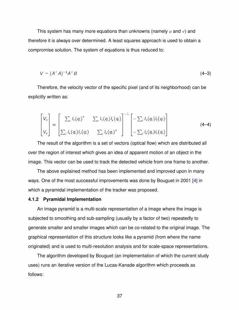
4.1.2 Pyramidal Implementation
An image pyramid is a multi-scale representation of a image where the image is
subjected to smoothing and sub-sampling (usually by a factor of two) repeatedly to
generate smaller and smaller images which can be co-related to the original image. The
graphical representation of this structure looks like a pyramid (from where the name
originated) and is used to multi-resolution analysis and for scale-space representations.
The algorithm developed by Bouguet (an implementation of which the current study
uses) runs an iterative version of the Lucas-Kanade algorithm which proceeds as
follows:
37
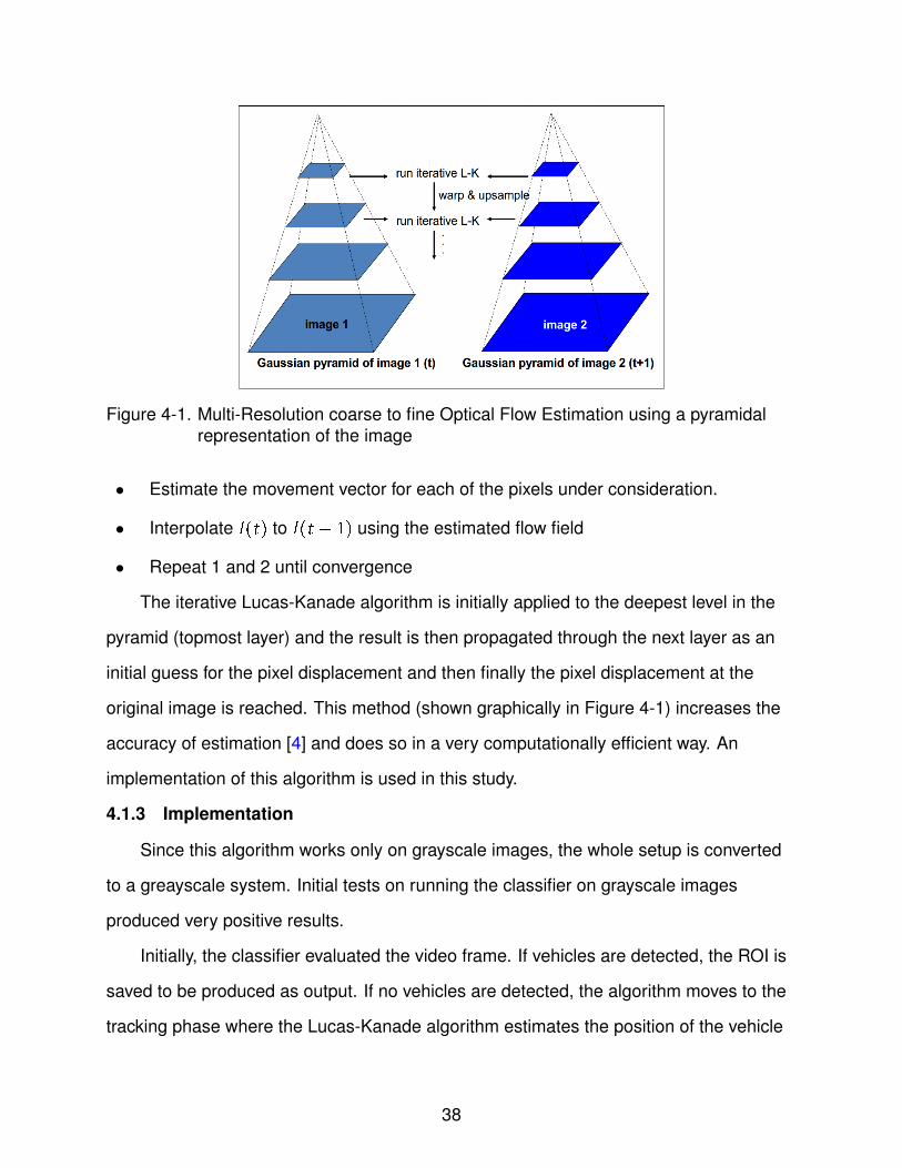
Figure 4-1. Multi-Resolution coarse to fine Optical Flow Estimation using a pyramidalrepresentation of the image
• Estimate the movement vector for each of the pixels under consideration.
• Interpolate I (t) to I (t + 1) using the estimated flow field
• Repeat 1 and 2 until convergence
The iterative Lucas-Kanade algorithm is initially applied to the deepest level in the
pyramid (topmost layer) and the result is then propagated through the next layer as an
initial guess for the pixel displacement and then finally the pixel displacement at the
original image is reached. This method (shown graphically in Figure 4-1) increases the
accuracy of estimation [4] and does so in a very computationally efficient way. An
implementation of this algorithm is used in this study.
4.1.3 Implementation
Since this algorithm works only on grayscale images, the whole setup is converted
to a greayscale system. Initial tests on running the classifier on grayscale images
produced very positive results.
Initially, the classifier evaluated the video frame. If vehicles are detected, the ROI is
saved to be produced as output. If no vehicles are detected, the algorithm moves to the
tracking phase where the Lucas-Kanade algorithm estimates the position of the vehicle
38
based on the detections in the previous frame. The Lucas-Kanade algorithm requires an
initial estimate of the object position (i.e initial pixels of interest) for estimating the
movement of the object. This initial estimate is obtained by setting the corner points of
the rectangle which bounds the vehicle region. A schematic of the process is shown in
Figure 4-2:
Figure 4-2. Schematic showing the algorithmic flow of the Tracking Process
4.2 Distance Estimation
Usually, the process of determining the distance of an object using a single
(monocular) vision system is purely an estimation process. In order to ascertain
accurate measurements of range information pertaining to a particular scene a stereo
rig (a system of two cameras viewing the scene from different points of view) is required.
But a major drawback of using stereo based methods is that they are computationally
taxing and therefore not suitable for a real time system.
Thus, methods for effectively estimating range information from a single camera
have been researched widely. Most of these methods use some sort of assumption,
either from a scene point of view (i.e. the camera is stationary) or from the object point
of view (i.e. assuming some known information about the object). Another major
39

assumption is that the transformation equations use a so called pin-hole camera model.
This model is represented by the following equation.
u
v
1
=
fx ∗ s; 0; cx
0; fy ∗ s; cy
0; 0; 1
r11; r12; r13; t1
r21; r22; r23; t2
r31; r32; r33; t3
X
Y
Z
1
(4–5)
where u and v represent a point in 2-D camera space. fx and fy are the focal
lengths (expressed in pixel related units). (cx , cy) represent a principal point, generally
the image center. The second 4x4 matrix is the rotation matrix which indicates the
rotation of the camera center with respect to the object center. The fourth column of the
matrix represent the translational element which represent the relative motion between
the camera and the object. The conversion factor s is the factor that transforms pixel
related units to millimeters (real world units).
The matrix containing the focal lengths and the principal point is called the intrinsic
matrix. This matrix is constant for every camera (which works on normal zoom) and
does not vary with the type of scene viewed. The second 4x4 matrix is called the
extrinsic matrix. This matrix gives information about the camera center with respect to
the world coordinate system and the heading of the camera (i.e the translation). Errors
resulting from distortion and misaligned lenses are not considered in this study.
The perspective pin-hole camera model described above is used to estimate the
distance of a vehicle detected in the video frame. Since the video is processed frame by
frame, the distance is estimated at every timestep. The following assumptions are made
in context of the current scenario for distance estimation.
• The world coordinate center is fixed at the camera center. This means that theextrinsic parameters will not have an effect on the transformation from 3-D pointsto 2-D pixels.
40

• The Z axis of the camera is along the line of the road. There is no yaw or roll anglebetween the road and the camera.
• Highway lanes have negligible slopes. Therefore, the pitch angle is also zero.
• Estimates for the width and height of a typical car are known and all vehicles havecomparable sizes.
Thus, given the typical width and height of a standard car W and H, and the width
and height of the detected Region of interest (ROI) in pixel related coordinates w and h,
one can estimate the distance of the car by the following two equations.
Z1 =s ∗ f ∗W
wZ2 =
s ∗ f ∗ Hh
(4–6)
where f is the average of fx and fy .
Thus, the distance estimate of a detected vehicle, updated at every timestep for
every detected vehicle is the average of Z1 and Z2. Therefore, a complete multi-vehicle
detction and tracking system with range estimation using a monocular vision system can
be implemented as shown in Figure 4-3.
4.3 Summary
This chapter delineated the theory behind the Lucas-Kanade Optical flow based
tracking algorithm along with Distance estimation using a pin-hole camera model. The
integration of a pyramidal implementation of the Lucas-Kanade algorithm to the actively
trained classifier for enhanced real time vehicle tracking is also explained. Furthermore,
a fully real time system able to robustly detect and track vehicles and also estimate,
fairly accurately, the range information of detected vehicles is outlined using a
schematic. This system can be implemented in a standard vehicle for enhanced driver
safety or in autonomous vehicles as a resource for classifying vehicles and as a
cognitive information tool for sensing and perception.
41

Figure 4-3. Algorithmic flow of the complete Detection and Tracking Process
42

CHAPTER 5EVALUATION AND DISCUSSION
The process of evaluating the designed system involves running the actively trained
classifier on specific (Static and Real Time) datasets and judging its performance based
on True Positive Detections and False Positive Detections. False Negatives are not of
much importance to this study because the True Positives give an empirical measure of
False Negative Detections. The results of the evaluation is comprehensively discussed
based on specifically defined evaluation parameters which present the system’s
robustness, sensitivity, recall, scalability and specificity. A comparison between the
actively trained and passively trained classifier is also given. The process of
implementing the full multi-vehicle detection and tracking system in a real time scenario
is presented. Finally, the results are summarized and the scope for future work is
outlined.
5.1 Datasets
5.1.1 Caltech 2001/1999 Static Image Database
This dataset consists of 1155 different images of the rear view of cars and was
compiled initially in 1999 and then modified in 2001. Most of the images have viewpoints
which are very close to the camera (unlike the case for most of the training examples)
and also consists of some models of cars which are old. This dataset has been widely
used in conjunction with testing a variety of vision based detection algorithms and serve
as a benchmark in static image testing. An example image is shown in Figure 5-1. This
dataset can be publicly accessed at the Computational Vision page at
www.vision.caltech.edu.
5.1.2 mvBlueFOX Test Data
This dataset consists of 362 frames of video collected using the mvBlueFOX
camera (which is used in this specific application) using the test rig. The frames consists
of a combination of frames collected at daytime and at low lightning conditions. The first
43

Figure 5-1. Caltech 2001/1999 Static Image Data Example
350 frames consist of consecutive frames collected at daytime with one vehicle of
interest in each frame and the next 12 frames consist of consecutive frames collected
during sunset with two vehicles of interest in each frame. All the frames were annotated
for true positives and set aside for testing. A screenshot of the Test Data is shown in
Figure 5-2:
Figure 5-2. Real Time test data captured using the test rig. This frame belongs to thedaytime set
The test rig consisted of an initially calibrated camera (Matrix Vision
mvBlueFOX-120a for which the intrinsic parameters are known) rigidly attached to the
top of the dashboard of a vehicle above the center console. The axis (z-axis) of the
44

camera was kept parallel to the road and the lens was adjusted at normal zoom. The
camera was attached to a laptop via USB and was operated by a human for specific
tasks (Data Collection, Capture and Testing).
5.2 Evaluation Parameters
The desired outcome of testing the classifier is the quantification of the classifier’s
robustness, sensitivity, specificity, scalability, and recall in terms of numerical values.
Most studies on vehicle detection using vision quantify their results by initially cropping
the image and normalizing them to a specific view and running the classifier on these
pre-processed images. This method, even though, has higher accuracy and report lower
false positives, does not account for robustness and scalability. Although, more recent
studies have come up with parameters to evaluate accuracy and recall in real time
systems, they do not offer numerical values for quantifying precision, robustness, and
specificity. The following parameters have been used in this study to evaluate the
classifiers in terms of accuracy, robustness, recall, sensitivity, and scalability.
• True Detection Rate (TDR) is measured by dividing the number of truly detectedvehicles by the total number of vehicles. This parameter gives a measure ofaccuracy and recall.
TDR =True Positives (No. of detected vehicles)
Actual No. of vehicles(5–1)
• False Positive Rate (FPR) is obtained by dividing the number of false detections(false positives) by the total number of detected vehicles (True and False). Thisparameter is an estimate of the system’s precision and robustness.
FPR =No. of false detections
Actual No. of vehicles + False Detections(5–2)
• Average True Detection per Frame (ATF) is the number of true positives (detected)divided by the total number of frames processed. This is a measure of sensitivity ofthe system.
ATF =True Positives
Total number of frames(5–3)
45

• Average False Detection per Frame (AFF) is measured by dividing the number offalse positives by total number of frames processed. This quantity gives anumerical measure for robustness and specificity.
AFF =False Positives
Total number of frames(5–4)
• Average False Detection per Vehicle (AFV) is the total number of false detctionsdivided by the number of vehicles on the road. It indicates robustness andprecision.
AFV =False Positives
Total number of Vehicles(5–5)
The overall performance of the system in terms of the above mentioned parameters
gives us an estimate of the scalability of the system. This is a measure of how the
framework can be adapted to be used in more advanced and real time scenarios (like in
autonomous vehicles).
5.3 Static Dataset
The actively trained classifier was evaluated on 1155 static images publicly available
and the performance characteristics described above are evaluated. A good classifier
performance on this dataset would justify its robustness and scalability The classifier
produced an accuracy of 92.98% with a False Detection Rate of 0.124. Some of the
detection results are consolidated in Figures 5-3 and 5-4.
In comparison the passively trained classifier returned an accuracy of 93.5% but
with a false positive rate of 0.35. This is the major tradeoff which has to be addressed
when choosing an Actively trained or Passively Trained classifier. The passively trained
classifier, as shown in the case of static datasets, performed marginally well but the
price in terms of False Positives is very high. This justifies the use of an Actively Trained
classifier in real time scenarios, as it performs much better in terms of precision and
robustness as explained below. A comparison of all the evaluation parameters for the
two classifiers is presented in Table 5-1.
46

Figure 5-3. Examples of True Positive Detections in Static Datset
Figure 5-4. Examples of false positives and missed detections - We can observe thatmost of the missed samples are due to the fact that the training datacontained examples exclusively from an real time dataset. The training datamodel did not contain many examples of cars very close to the camera.
Table 5-1. Results on Static Dataset - Active-Passive ComparisionParameter Passive Classifier Active ClassifierTrue Detection Rate 93.5% 92.8%False Positive Rate 0.35 0.124Average True per Frame 0.985 0.98Average False per Frame 0.48 0.16Average False per Vehicle 0.45 0.138
47

Although, the accuracy of the Passive classifier is higher, the false positive rate is
almost three times as much as the Active classifier. Also, average false detections per
frame and per vehicle is four times higher when compared to the Active classifier. Thus,
one can confidently argue that the Active classifier performs much better in terms of
precision in static tests. Further, in Figure 5-5 a Receiver Operating Curve (ROC) is
plotted between the True Detections and False Positives Rate. This graph gives an idea
of the classifiers sensitivity (accuracy) with respect to specificity (the measure of how
true the classifications are).
Figure 5-5. The ROC curves for Actively and Passively Trained Classifiers
In terms of an ROC curve, a better classifier is the one which is more justified
towards the left of the line which divides the graph at 45 degrees. From the above curve,
we can easily infer that the Actively Trained classifier is much stronger in performance in
terms of specificity than the Passive classifier. Therefore, in static tests one can
conclude that the Active classifier performs much better in terms of precision and
robustness although there is a small tradeoff in terms of accuracy.
48

5.4 Real Time Dataset
The Actively Trained classifier was evaluated on 362 frames of real time test data.
Most of the data was comprised of consecutive frames of video stream taken during
good lightning conditions (sunny). Some frames were also obtained at low lighting
conditions (half an hour before sunset) to evaluate the performance of the classifier in
such conditions. It was found that the classifier returned an accuracy of 98.8% (i.e. 372
hits out of 376 vehicles). The false positive rate was 0.124. An average frame rate of
15.6 frames per second was achieved in testing on an Intel i5 Processor (2.3 Ghz Quad
core) with 4GB RAM. The process utilized no multi-threading or GPU optimization.
Previous studies support the fact that using GPU optimization of vision based algorithms
could speed up processes by more than 10 times. Some examples of detected results
are shown in Figures 5-6 and 5-7.
Figure 5-6. Examples of True Positive Detections in Real Time Test set. The first columnshows two frames in very low lighting conditions where both the cars weredetected accurately. The second and third columns shows two consecutiveframes each where the car was detected in both the cases. The real time setperformed better than the static data set since the training data wascaptured using the same test rig
A graphic illustration of the number of vehicles detected at each frame compared to
the actual number of vehicles is presented in Figure 5-8. One can observe that the
49

Figure 5-7. Examples of false positives and missed detections. We can observe that inthe first two pictures, false positive are due to other vehicles and incomingvehicles. In the third case, low lighting prevented detection of one car and inthe final case there were two detections on the same car
Figure 5-8. Graph illustrating the number of vehicles detected at each frame and falsepositives. This is compared to the actual number of vehicles in the scene
50

classifier maintains the track of detected vehicles with considerable efficiency. But, in
some frames, the track of the vehicle is completely lost (i.e a missed detection). Thus,
integrating a feature based tracker would fully eliminate the problem of missed
detections (even though they occur very rarely). We can also observe that the false
detection rate is not continuous for every two frames. There is no false positive which
was detected over two frames. This gives an incentive to modify the feature based
tracker to only track regions which have been detected over two frames. Thus, the whole
framework was modified to address this issue.
Another observation made was that, from Figure 5-7, one can infer that some of the
false positives are actually detection over the same window but with a larger area.
These detections can be checked for and double detections in the same vicinity can be
accounted for by tweaking the algorithm to skip over previously detected regions as the
detection window is made larger. Finally, the highlight of the test was the fact that the
Average False positives per Frame for the recognizer was found out to be 0.12. This
means that when the classifier is integrated with a tracker, this value is low enough so
that it is not consistent to create wrong tracks. This highlights the scalability of the
classifier to more sophisticated frameworks.
The passively trained classifier was also evaluated using the real time data set. In
contrast to the static dataset, the classifier in this case produced a lower (almost equal)
accuracy of 98.6% when compared to the Actively trained classifier. The rate of false
detections was 0.24. This was lower than the static false positive rate but almost twice
as much when compared to the Actively Trained classifier. The evaluation parameters
are shown in Table 5-2:
One can observe that the Passive classifier returned an almost comparable
accuracy to the Active classifier. Also, the average true detections per frame for both the
classifiers are the same. This validates the use of the Haar-like feature based
Viola-Jones algorithm for vision based vehicle detection. But, the false positive rate
51
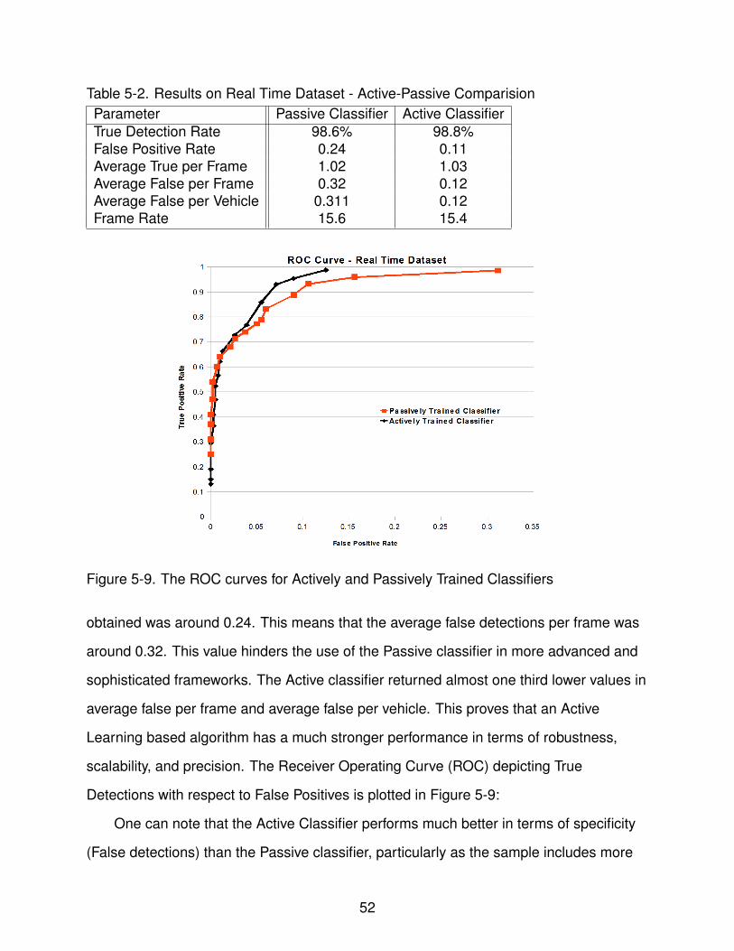
Table 5-2. Results on Real Time Dataset - Active-Passive ComparisionParameter Passive Classifier Active ClassifierTrue Detection Rate 98.6% 98.8%False Positive Rate 0.24 0.11Average True per Frame 1.02 1.03Average False per Frame 0.32 0.12Average False per Vehicle 0.311 0.12Frame Rate 15.6 15.4
Figure 5-9. The ROC curves for Actively and Passively Trained Classifiers
obtained was around 0.24. This means that the average false detections per frame was
around 0.32. This value hinders the use of the Passive classifier in more advanced and
sophisticated frameworks. The Active classifier returned almost one third lower values in
average false per frame and average false per vehicle. This proves that an Active
Learning based algorithm has a much stronger performance in terms of robustness,
scalability, and precision. The Receiver Operating Curve (ROC) depicting True
Detections with respect to False Positives is plotted in Figure 5-9:
One can note that the Active Classifier performs much better in terms of specificity
(False detections) than the Passive classifier, particularly as the sample includes more
52

examples with higher true detections. Thus, it can be argued that the Active classifier is
much more robust and sensitive to noise than the Passive classifier thereby validating its
use in real time platforms like in Intelligent Vehicles.
5.5 Implementation in a Real Time Scenario
The complete multi-vehicle detection and tracking system with integrated
Lucas-Kanade tracker and Distance estimation, outlined in Figure 4-10, was
implemented in a real time scenario using the test rig explained earlier. The testing
conditions were sunny with light traffic. The algorithm could only run in grayscale as the
Tracking module only worked with grayscale images. Some frames from the run are
shown and explained in Figures 5-10 and 5-11:
Figure 5-10. A frame from the full system implementation showing a detected car with itsdistance estimate
5.6 Summary
This chapter provided the proof of concept implementaion of the Actively trained
Viola-Jones classifier for the purpose of real time vehicle detection. The classifier was
evaluated on publicly available static image datasets as well as on real time video
53

Figure 5-11. The next frame where the car was not detected but was tracked from theprevious frame. Thus the distance estimate yields the same value. Thedistance is measured as 498.67 inches which scales to around 12.5meters.
stream collected using the test rig. The classifier was then compared to the Passively
trained classifier based on some specific evaluation criteria and results were presented.
The full implementation of the multi-vehicle detection and tracking system complete with
a feature tracker and distance estimation on a real time scenario is also presented.
54

CHAPTER 6CONCLUSIONS AND FUTURE WORK
The idea of this thesis was to present a vision based vehicle detection and tracking
system which can be implemented in real time systems such as in intelligent vehicles
and autonomous cars. The main challenge in addressing this issue was to create a
robust, reliable system which was simple to implement. A machine learning based
approach was devised to solve this problem where a cascade of classifiers were trained
based on Adaboost (working on Rectangular Haar-like features in an image) to rapidly
detect Regions of Interest (ROIs) corresponding to cars in a video frame. This classifier
was then retrained using Query by Misclassification to produce an Active classifier which
was much more sensitive to noise.
This classifier was then integrated with a Feature based (Lucas-Kanade) tracker
along with a distance estimation algorithm (monocular vision based) to build a complete
multi-vehicle detection and tracking system. This framework was evaluated on static and
real time data and the performance was found to be highly satisfactory with 98%
detection rates at 16 frames per second. The performance characteristics of this system
enables it to be deployed in more sophisticated and advanced frameworks.
Going further, a variety of principles could be improved upon. A significant
improvement might arise from using a very large training dataset representing all lighting
conditions and vehicle types. The only drawback of using a large dataset is the amount
of human capital involved in annotating the ground truth. Therfore, the next step would
be to devise a mechanism which could automatically annotate the Region of Interest by
using some classical approaches (which are very robust, but do not perform in real time)
to initially classify vehicles. This method could also be used to selectively sample the
independent dataset used for Active Learning and query it for retraining. Integration of
lane detection, trajectory learning and pedestrian detection are some other key
55

advances which could be integrated into the current system for transforming the system
into a complete enhanced Active safety system.
56

REFERENCES
[1] Balcones, D, Llorca, D, and Sotelo, M. “Real-time vision-based vehicle detection forrear-end collision mitigation systems.” Computer Aided Systems Theory (2009):320–325.
URL http://www.springerlink.com/index/UU7VU34310825343.pdf
[2] Bensrhair, A and Bertozzi, M. “A cooperative approach to vision-based vehicledetection.” Intelligent Transportation Systems Conference Proceedings (2001):209–214.
URLhttp://ieeexplore.ieee.org/xpls/abs_all.jsp?arnumber=948657
[3] Betke, Margrit, Haritaoglu, Esin, and Davis, Larry S. “Real-time multiple vehicledetection and tracking from a moving vehicle.” Machine Vision and Applications 12(2000).2: 69–83.
URL http://www.springerlink.com/openurl.asp?genre=article\&id=doi:10.1007/s001380050126
[4] Bouguet, Jean-yves. “Pyramidal Implementation of the Lucas Kanade FeatureTracker Description of the algorithm.” Tech. Rep. 2, 2001.
[5] Bouttefroy, P.L.M., Bouzerdoum, A., Phung, S.L., and Beghdadi, A. “VehicleTracking Using Projective Particle Filter.” 2009 Sixth IEEE International Conferenceon Advanced Video and Signal Based Surveillance. IEEE, 2009, 7–12.
URL http://ieeexplore.ieee.org/xpls/abs_all.jsp?arnumber=5279471’escapeXml=’false’/>
[6] Cao, Xianbin, Lan, Jinhe, Yan, Pingkun, and Li, Xuelong. “KLT Feature BasedVehicle Detection and Tracking in Airborne Videos.” 2011 Sixth InternationalConference on Image and Graphics. IEEE, 2011, 673–678.
URL http://ieeexplore.ieee.org/xpls/abs_all.jsp?arnumber=6005950’escapeXml=’false’/>
[7] Chen, Yen-Lin, Wu, Bing-Fei, and Fan, Chung-Jui. “Real-time vision-based multiplevehicle detection and tracking for nighttime traffic surveillance.” 2009 IEEEInternational Conference on Systems, Man and Cybernetics. IEEE, 2009,3352–3358.
URL http://ieeexplore.ieee.org/xpl/articleDetails.jsp?reload=true\&arnumber=5346191\&contentType=Conference+Publications
[8] Choi, Jaesik. “Realtime On-Road Vehicle Detection with Optical Flows andHaar-Like Feature Detectors.” (2012).
57

URL https://www.ideals.illinois.edu/handle/2142/30794
[9] Dallalzadeh, Elham and Guru, D. S. “Feature-based tracking approach for detectionof moving vehicle in traffic videos.” Proceedings of the First InternationalConference on Intelligent Interactive Technologies and Multimedia - IITM ’10. NewYork, New York, USA: ACM Press, 2010, 254–260.
URL http://dl.acm.org/citation.cfm?id=1963564.1963609
[10] Firouzi, H and Najjaran, H. “Real-time monocular vision-based object tracking withobject distance and motion estimation.” IEEE ASME International Conference onAdvanced Intelligent Mechatronics (AIM) . . . (2010).
URLhttp://ieeexplore.ieee.org/xpls/abs_all.jsp?arnumber=5695936
[11] Garcı́a, RIR and Shu, D. “Vision based Vehicle Tracking using a high anglecamera.” Tech. Rep. figure 1, ????
URL http://www.ces.clemson.edu/˜stb/ece847/projects/VISION_BASED_VEHICLE_TRACKING.pdf
[12] Han, S, Han, Youngjoon, and Hahn, Hernsoo. “Vehicle Detection Method UsingHaar-Like Frature on Real Time System.” World Academy of Science, Engineeringand Technology (2009): 455–459.
URL http://citeseerx.ist.psu.edu/viewdoc/download?doi=10.1.1.192.8220\&rep=rep1\&type=pdf
[13] Holub, Alex, Perona, Pietro, and Burl, Michael C. “Entropy-based active learning forobject recognition.” 2008 IEEE Computer Society Conference on Computer Visionand Pattern Recognition Workshops (2008): 1–8.
URL http://ieeexplore.ieee.org/lpdocs/epic03/wrapper.htm?arnumber=4563068
[14] Jones, MJ and Viola, P. “Robust real-time object detection.” Workshop on Statisticaland Computational Theories of Vision (2001).February.
URLhttps://www.hpl.hp.com/techreports/Compaq-DEC/CRL-2001-1.html
[15] Kapoor, Ashish, Grauman, Kristen, Urtasun, Raquel, and Darrell, Trevor. “ActiveLearning with Gaussian Processes for Object Categorization.” 2007 IEEE 11thInternational Conference on Computer Vision (2007): 1–8.
URL http://ieeexplore.ieee.org/lpdocs/epic03/wrapper.htm?arnumber=4408844
58

[16] Khalid, Zebbara, Mazoul, Abdenbi, and Ansari, Mohamed El. “A new vehicledetection method.” International Journal of Advanced Computer Science andApplications (2011): 72–76.
URL https://www.thesai.org/Downloads/SpecialIssueNo3/Paper12-Anewvehicledetectionmethod.pdf
[17] Kim, Giseok and Cho, Jae-Soo. “Vision-based vehicle detection and inter-vehicledistance estimation for driver alarm system.” Optical Review 19 (2012).6: 388–393.
URLhttp://www.springerlink.com/index/10.1007/s10043-012-0063-1
[18] Kobilarov, M., Sukhatme, G., Hyams, J., and Batavia, P. “People tracking andfollowing with mobile robot using an omnidirectional camera and a laser.”Proceedings 2006 IEEE International Conference on Robotics and Automation,2006. ICRA 2006. (2006).May: 557–562.
URL http://ieeexplore.ieee.org/lpdocs/epic03/wrapper.htm?arnumber=1641769
[19] Liu, Chendong; Zhang Yunzhou, Meng; Wu. “Motion vehicle tracking based onmulti-resolution optical flow and multi-scale Harris corner detection.” 2007 IEEEInternational Conference on Robotics and Biomimetics (ROBIO). IEEE, 2007,2032–2036.
URL http://ieeexplore.ieee.org/xpls/abs_all.jsp?arnumber=4522480’escapeXml=’false’/>
[20] Lucas, Bruce D. Generalized Image Matching by a method od differences. Ph.D.thesis, 1981.
[21] Miller, R., Bebis, G., and DiMeo, D. “A real-time precrash vehicle detection system.”Sixth IEEE Workshop on Applications of Computer Vision, 2002. (WACV 2002).Proceedings. (????): 171–176.
URL http://ieeexplore.ieee.org/lpdocs/epic03/wrapper.htm?arnumber=1182177
[22] Nilsson, Nils J. Introduction to machine learning. 2004.
URL http://scholar.google.com/scholar?hl=en\&btnG=Search\&q=intitle:INTRODUCTION+TO+MACHINE+LEARNING+AN+EARLY+DRAFT+OF+A+PROPOSED+TEXTBOOK+Department+of+Computer+Science#0http://books.google.com/books?hl=en\&lr=\&id=1k0_-WroiqEC\&oi=fnd\&pg=PR13\&dq=INTRODUCTION+TO+MACHINE+LEARNING\&ots=p90K-RcLuL\&sig=nQgzbYlsUF8gX9djK_-MEWk_2jg
59

[23] Olsson, Fredrik. “A literature survey of active machine learning in the context ofnatural language processing.” Swedish Institute of Computer Science (2009):134–138.
[24] Papageorgiou, Constantine and Poggio, Tomaso. “A trainable system for objectdetection.” International Journal of Computer Vision 38 (2000).1: 15–33.
URL http://www.springerlink.com/index/WW5UT522540L672R.pdf
[25] Parekh, Kayton B. A Computer Vision Application to accurately estimate objectdistance. Ph.D. thesis, ????
URL http://digitalcommons.macalester.edu/cgi/viewcontent.cgi?article=1018\&context=mathcs_honors
[26] Rezaee, Hamideh, Aghagolzadeh, Ali, and Seyedarabi, Hadi. “Vehicle tracking byfusing multiple cues in structured environments using particle filter.” 2010 IEEEAsia Pacific Conference on Circuits and Systems. IEEE, 2010, 1001–1004.
URL http://ieeexplore.ieee.org/xpls/abs_all.jsp?arnumber=5775069’escapeXml=’false’/>
[27] Sayanan Sivaraman, Mohan M. Trivedi. “Combining Monocular and Stereo-Visionfor Real-Time Vehicle Ranging and Tracking on Multilane Highways.” 14thInternational IEEE Conference on Intelligent Transportation Systems. 2011,1249–1254.
URL http://130.203.133.150/viewdoc/summary;jsessionid=FF2E2F450D2498414806725AE886A282?doi=10.1.1.228.3732
[28] Sivaraman, Sayanan and Trivedi, Mohan M. “Active learning for on-road vehicledetection: a comparative study.” Machine Vision and Applications (2011).
URLhttp://www.springerlink.com/index/10.1007/s00138-011-0388-y
[29] Sivaraman, Sayanan and Trivedi, Mohan Manubhai. “Active learning based robustmonocular vehicle detection for on-road safety systems.” 2009 IEEE IntelligentVehicles Symposium. IEEE, 2009, 399–404.
URLhttp://ieeexplore.ieee.org/xpls/abs_all.jsp?arnumber=5164311
[30] ———. “A General Active-Learning Framework for On-Road Vehicle Recognitionand Tracking.” IEEE Transactions on Intelligent Transportation Systems 11(2010).2: 267–276.
URL http://ieeexplore.ieee.org/lpdocs/epic03/wrapper.htm?arnumber=5411825
60

[31] Subramanian, Anbumani. Image segmentation and range estimation using amoving-aperture lens. Ph.D. thesis, 2001.
URL http://citeseerx.ist.psu.edu/viewdoc/download?doi=10.1.1.5.9656\&rep=rep1\&type=pdf
[32] Tsai, Yi-Min, Tsai, Chih-Chung, Huang, Keng-Yen, and Chen, Liang-Gee. “Anintelligent vision-based vehicle detection and tracking system for automotiveapplications.” 2011 IEEE International Conference on Consumer Electronics(ICCE). IEEE, 2011, 113–114.
URL http://www.researchgate.net/publication/224222737_An_intelligent_vision-based_vehicle_detection_and_tracking_system_for_automotive_applications
[33] Wu, Bing-fei, Kao, Chih-Chung, Liu, Chih-Chun, Fan, Chung-Jui, and Chen,Chao-Jung. “The vision-based vehicle detection and incident detection system inHsueh-Shan tunnel.” 2008 IEEE International Symposium on Industrial Electronics.IEEE, 2008, 1394–1399.
URLhttp://ieeexplore.ieee.org/xpls/abs_all.jsp?arnumber=4677196
[34] Yamaguchi, K., Kato, T., and Ninomiya, Y. “Vehicle Ego-Motion Estimation andMoving Object Detection using a Monocular Camera.” 18th InternationalConference on Pattern Recognition (ICPR’06) (2006): 610–613.
URL http://ieeexplore.ieee.org/lpdocs/epic03/wrapper.htm?arnumber=1699915
[35] Yong, Xi, Zhang, L, and Song, Zhangjun. “Real-time vehicle detection based onHaar features and Pairwise Geometrical Histograms.” IEEE InternationalConference on Information and Automation (2011).June: 390–395.
URLhttp://ieeexplore.ieee.org/xpls/abs_all.jsp?arnumber=5949023
61
BIOGRAPHICAL SKETCH
Vishnu Karakkat Narayanan was born in Kerala in South India. He received his M.S.
in mechanical engineering from the University of Florida, Gainesville in May 2013 with a
minor in electrical and computer engineering. He had received his BTech. in mechanical
engineering from Amrita University, Coimbatore, India in May 2011. His research is
focused of applications of Computer Vision and Machine Learning to real time systems.
He developed an interest and passion for Machine Learning and Computer Vision,
during his final year of undergraduate study while working on his Bachelors thesis on
Machine Learning based Manufacturing Optimization. He plans to pursue a doctorate
degree in the same field and move on to academia.
62