velocity measurements in a convective flow by holographic interferometry

Velocity measurements in aconvective flow by holographic interferometry

Nieves Andres, Pilar Arroyo, and Manuel Quintanilla

A holographic interferometry technique has been developed that can be used to measure the threecomponents of the velocity field in a whole plane of a fluid flow simultaneously. The light scattered froman illuminated fluid plane is recorded on a hologram. Several interferograms are obtained in thereconstruction of the hologram. Each interferogram is automatically analyzed and produces quantita-tive information about one velocity component. Parameters that affect the quality of the interferogramsare analyzed. The technique is demonstrated in a Rayleigh–Benard convective flow. Holographicinterferometry and particle image velocimetry techniques are compared. © 1997 Optical Society ofAmerica

Key words: Laser velocimetry, fluid velocimetry, holographic interferometry.

1. Introduction

Particle image velocimetry ~PIV! is a technique usedfor the simultaneous measurement of velocity fieldsin extended regions of fluid flows.1 It originatedfrom the speckle photography techniques that wereused to measure full-field in-plane displacements ofsolid surfaces.2 The first applications in fluid me-chanics were reported in 1977,3–5 where velocityfields in one-dimensional flows were measured. Re-ports of two velocity component measurements intwo-dimensional flows6,7 quickly followed. Sincethen PIV has developed rapidly and turned into awidespread and mature technique.

Holographic interferometry ~HI! is another classictechnique for the measurement of displacements anddeformations of solid surfaces.8 The first applica-tion of this technique in fluid mechanics was alsoreported in 1977,9 where one velocity componentfields were measured. But HI did not follow thesame rapid development as PIV. To date, HI as avelocimetry technique has been applied only to aRayleigh–Benard convective flow,10–12 and it hasbeen used more as a flow visualization techniquethan as a means of quantitatively measuring the ve-

The authors are with the Departamento de Fısica Aplicada,Facultad de Ciencias, Universidad de Zaragoza, Ciudad Universi-taria, 50009-Zaragoza, Spain.

Received 9 October 1996; revised manuscript received 26 Feb-ruary 1997.

0003-6935y97y276997-11$10.00y0© 1997 Optical Society of America

locity field. Furthermore, only one velocity compo-nent information has been reported in these studies.The slow development of HI can be explained by thefact that it can require the use of more powerfullasers than PIV since the holographic recording ma-terial used for HI has less sensitivity than the pho-tographic recording film used in PIV. In addition,the exposure times are approximately 50 timessmaller in HI than in PIV, thus noticeably decreasingthe energy of each exposure when a continuous laseris used. Recent developments in laser technologyhave made possible the use of pulsed lasers with highenergy that make the application of HI more feasible.In fact, nowadays even PIV is sometimes imple-mented with a holographic ~instead of photographic!method to record the flow.13,14 Another drawback ofHI is that it naturally provides measurements of onlyone ~out-of-plane! velocity component compared withthe two ~in-plane! velocity components that can bemeasured with PIV. However, HI has been shownto be capable of measuring the three components ofsolid-surface displacement when an appropriate re-cording and reconstruction of the hologram isused.15,16

The purpose of this study is to investigate the fea-sibility of HI to measure the three components of thevelocity field in a whole plane of a fluid flow simul-taneously. In the following, we present some resultsobtained in a Rayleigh–Benard convective flow as ameans of demonstrating the applicability of the tech-nique. Emphasis is placed on specific questions re-lated to the performance of HI as a practicaltechnique for the quantitative measurement of sev-

20 September 1997 y Vol. 36, No. 27 y APPLIED OPTICS 6997

eral velocity components. A concerted effort hasbeen made to optimize and automate HI, which wecompare with PIV whenever possible.

2. Holographic Interferometry

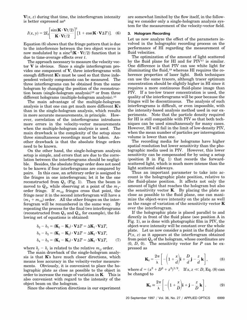
HI refers, generally speaking, to any technique forinterferometric comparison of two or more holograph-ically reconstructed waves. These waves, whichrepresent the light scattered or transmitted to thehologram by some object, are recorded sequentially intime. If the object was slightly changed betweensuccessive exposures of the hologram, the interfero-metric comparison provides information about thosechanges. When one measures flow velocities, theremust be something like a rough surface inside thefluid, which is achieved by illuminating a fluid plane,previously seeded with diffusing particles, as inPIV.17 Light scattered from the particles is the ob-ject wave, which is recorded at least twice at fixedtime intervals DT also as in PIV. Changes in thisobject come from the local displacement d of the trac-ers during time intervals. This displacement is re-lated to the local fluid velocity such that d 5 VDT.Here, the main differences between PIV and HI arethat in HI the object wave is recorded holographicallyinstead of photographically and the recording filmcan be placed in any position and orientation relativeto the illuminated plane ~Fig. 1!. The holographicrecording requires a reference beam that is conve-niently taken as a collimated beam that covers thewhole holographic plate.

The hologram so recorded is then reconstructedwith a pointwise beam, which travels in the directionopposite to the reference beam and has a diameter ofonly a few millimeters. In this way, a real image ofthe illuminated fluid plane, which appears to be over-laid by interference fringes, is obtained. In the fol-

Fig. 1. Optical arrangement for measuring flow velocity fields byholographic interferometry.

6998 APPLIED OPTICS y Vol. 36, No. 27 y 20 September 1997

lowing, we refer to this image as an interferogram.The intensity on the interferogram can be expressed,for a doubly exposed hologram, as

I~x, z! 5 2I0@1 1 cos~K z VDT !#, (1)

where I0 is the intensity of the illuminated fluidplane, V~x, z! is the local velocity at the ~x, z! coordi-nates, and K 5 ~2pyl!@uo 2 ui# is the sensitivityvector, where uo and ui are unity vectors in the ob-servation and illumination directions, respectively.Here we note that the sensitivity vector has to becalculated within the fluid. Equation ~1! representsa fringe pattern since the intensity changes from 0 to4 I0 depending on the velocity. The maximum in-tensity is obtained where

K z VDT 5 2pm, m 5 0, 61, 62, . . . . (2)

The integer m is known as the interference fringeorder. Thus the brightest fringes correspond to ve-locities such that

VK 5 m2py~uKuDT !, (3)

where VK means the projection of V along the direc-tion of K. If u is the angle between uo and ui, Eq. ~3!can be rewritten as

VK 5 mly~2DT sin uy2!. (4)

In general, ui is the same throughout the fluidplane, whereas uo can change over the plane. If thehologram–fluid-plane distance is much larger thanthe fluid-plane dimensions, uo is constant and theinterferogram represents an isovelocity componentmap. The velocity component selected is the projec-tion along K, VK.

The quantitative analysis of the interferogram ismeant to provide the value of VK on the nodes of arectangular grid. One way of doing this is to locatethe fringe maxima positions for each fringe and as-sign them the corresponding velocity value accordingto Eq. ~3!. Then an interpolation process can be usedto determine the velocity on the grid nodes. Such aprocedure was recently used in a fast quantitativeanalysis of PIV photographs,18 where isovelocity com-ponent maps were obtained through an optical spa-tial filtering of the photograph.

Another way of analyzing the interferogram con-sists of directly obtaining at the grid nodes the valueof the term K z VDT, which is known as phase differ-ence d, since the interferogram intensity depends ond. According to Eq. ~1!, d can be obtained as

d~x, z! 5 arccosF I~x, z!

2I0~x, z!2 1G . (5)

In this case, I0~x, z! must be previously known andcan change over the fluid plane not only for purelygeometric reasons but also because of time-averageholography effects. Equation ~1! is valid when theobject is stationary during exposure time t. How-ever, when the object moves with a constant velocity

V~x, z! during that time, the interferogram intensityis better expressed as8

I~x, y! 5 2I0Fsin~K z Vty2!

K z Vty2 G2

@1 1 cos~K z VDT !#. (6)

Equation ~6! shows that the fringe pattern that is dueto the interference between the two object waves isnow modulated by a sinc2~K z Vty2! function that isdue to time-average effects over t.

The approach necessary to measure the velocity vec-tor V is obvious. Since a single interferogram pro-vides one component of V, three interferograms withenough different K’s must be used so that three inde-pendent velocity components can be measured. Thethree interferograms can be obtained from the samehologram by changing the position of the reconstruc-tion beam ~single-hologram analysis!16 or from threedifferent holograms ~multiple-hologram analysis!.15

The main advantage of the multiple-hologramanalysis is that one can get much more different K’sthan in the single-hologram analysis, which resultsin more accurate measurements, in principle. How-ever, correlation of the interferograms introducesmore errors in the velocity-vector measurementswhen the multiple-hologram analysis is used. Themain drawback is the complexity of the setup sincethree simultaneous recordings must be taken. An-other drawback is that the absolute fringe ordersneed to be known.

On the other hand, the single-hologram analysissetup is simple, and errors that are due to the corre-lation between the interferograms should be negligi-ble. Besides, the absolute fringe order does not needto be known if four interferograms are compared bypairs. In this case, an arbitrary order is assigned tothe fringes in one interferogram; let it be the onereconstructed from Q1 ~Fig. 1!. Then the beam ismoved to Q2, while observing at a point of the m1-order fringe. If m12 fringes cross that point, thefringe near it in the second interferogram will have a~m1 1 m12! order. All the other fringes on the inter-ferogram will be renumbered in the same way. Byrepeating the process for the final two interferograms~reconstructed from Q3 and Q4, for example!, the fol-lowing set of equations is obtained:

d2 2 d1 5 ~K2 2 K1! z VDT 5 DK1 z VDT,

d3 2 d2 5 ~K3 2 K2! z VDT 5 DK2 z VDT,

d4 2 d3 5 ~K4 2 K3! z VDT 5 DK3 z VDT, (7)

where dj 2 di is related to the relative mij order.The main drawback of the single-hologram analy-

sis is that K’s have much closer directions, whichmeans less accuracy in the velocity-vector measure-ments. Obviously, it is convenient to place the ho-lographic plate as close as possible to the object inorder to increase the range of variation in K. This isalso convenient with regard to the intensity of theobject beam on the hologram.

Since the observation directions in our experiment

are somewhat limited by the flow itself, in the follow-ing we consider only a single-hologram analysis sys-tem for the measurement of the velocity-vector field.

3. Hologram Recording

Let us now analyze the effect of the parameters in-volved in the holographic recording process on theperformance of HI regarding the measurement offluid velocities.

The optimization of the amount of light scatteredby the fluid plane for HI and for PIV17 is similar.One difference is that PIV can use white light forilluminating the fluid,19 whereas HI requires the co-herence properties of laser light. Both techniquescan use the same tracers, although tracer optimumconcentration should be slightly higher in HI since itrequires a more continuous fluid-plane image thanPIV. If a too-low tracer concentration is used, thequality of the interferograms will be poor because thefringes will be discontinuous. The analysis of suchinterferograms is difficult, or even impossible, withthe intensity-based analysis method used in our ex-periments. Note that the particle density requiredfor HI is still compatible with PIV so that both tech-niques can be used simultaneously for many cases.However, HI will fail in the limit of low-density PIV,when the mean number of particles per interrogationvolume is lower than one.

The recording media for holograms have higherspatial resolution but lower sensitivity than the pho-tographic media used in PIV. However, this lowersensitivity can be compensated for by using a setup~position B in Fig. 1! that records the forward-scattered light, which is much more intense than thelight scattered sideways.

Thus an important parameter to take into ac-count is the holographic plate position, relative tothe fluid-plane position. It affects not only theamount of light that reaches the hologram but alsothe sensitivity vector K. By placing the plate asclose as possible to the fluid plane, one can maxi-mize the object-wave intensity on the plate as wellas the range of variation of the sensitivity vector Kover the interferogram.

If the holographic plate is placed parallel to anddirectly in front of the fluid plane ~see position A inFig. 1!, as is done with photographic film in PIV, theobject-wave intensity will be constant over the wholeplate. Let us now consider a point in the fluid planeP~x, z! as it appears at the interferogram obtainedfrom point Q0 of the hologram, whose coordinates are~0, D, 0!. The sensitivity vector for P can be ex-pressed as

K0 52p

l F2S1 1xdDi 1

Dd

j 2zd

kG , (8)

where d 5 ~x2 1 D2 1 z2!1y2. If x, z ,, D, Eq. ~8! canbe changed to

K0 >2p

l F2S1 1xDDi 1 j 2

zD

kG . (9)


Equation ~9! implies that the contribution of the Vxand Vy components to the phase difference in point Pis similar, whereas the contribution of the Vz compo-nent is much smaller.

When comparing two interferograms obtainedfrom two points of the plate, such as Q1 and Q2, withthe same z-coordinate ~L9! and a relative distance of2L, we obtained

DK1 5 K2 2 K1 >2p

l S22LD D

3 F~1 1 O$L2yD2%!i 1xD

j 1x~L9 2 z!

D2 kG , (10)

where O$L2yD2% represents the order of magnitude ofthe remaining terms. Equation ~10! implies that thephase difference between the two interferograms de-pends basically on Vx.

In the same way, when comparing two interfero-grams obtained from two points of the plate, such asQ2 and Q3, with the same x-coordinate ~L! and arelative distance of 2L9, we obtained

DK2 5 K3 2 K2 >2p

l S22L9

D D3 F2

z~L 1 x!

D2 i 1zD

j 1 ~1 1 O$L2yD2%!kG. (11)

Equation ~11! implies that the phase difference be-tween these two interferograms depends basically onVz.

Therefore when the holographic plate is placed inposition A, one can easily obtain Vx and Vz compo-nents by comparing two interferograms. Vy can beinferred only from the analysis of a single interfero-gram, if the absolute fringe orders are known and Vxand Vz have been measured. The accuracy of themeasurements depends on the order of magnitude ofthe velocity components and on the ratios LyD andL9yD. In general, the accuracy of Vy will be smallerthan the accuracy of Vx and Vz.

Let us now consider the holographic plate placed ina forward position, such as position B in Fig. 1, wherethe angle a between the mean observation vector ~inair! uo9 and the illumination vector ui is small andthe plate is perpendicular to uo9~b 5 a!. In this case,the object-wave intensity will not be uniform over theplate but will be much higher than in position A.The intensity increases with a decrease of the dis-tance between the object and the plate and with adecrease in angle a. For particular values such as a5 20°, D ; 160 mm, and 2L ; 40 mm, the object-wave intensity is twice as large at point Q1 than it isat point Q2 of the plate. The intensity can be mademore uniform by increasing b but an increase in balso implies a decrease in the range of variation of K~unless the size of the plate is increased! and in theintensity value.


In this configuration and assuming that x, z ,, D,the sensitivity vector K0 can be expressed as

K0 >2p

l F2S1 1xD

sin2 a 2 cos aDi1 S1 1

xD

cos aDsin aj 2 S1 1xD

cos aD zD

kG ,

(12)

which agrees with Eq. ~9! for a 5 90. For small a,Eq. ~12! shows that the phase difference is dominatedby the Vy component.

The comparison of two interferograms obtainedfrom two different points on the holographic plateproduces the following variation in K:

DK1 >2p

l S22LD DHS1 1

2xD

cos a 1 O$L2yD2%Dsin ai

2 FxD

cos 2a 1 cos a~1 1 O$L2yD2%!G j

1x~L9 2 z!

D2 sin akJ , (13)

DK2 >2p

l S22L9

D DH~D cos a 2 L sin a 2 x!z

D2 i

1 ~D sin a 1 L cos a!z

D2 j

1 S1 1xD

cos a 1 O$L2yD2%DkJ , (14)

where DK1 corresponds to Q1 and Q2 and DK2 corre-sponds to Q2 and Q3. Thus, for small a, the phasedifference between interferograms 1 and 2 dependsmainly on Vy, whereas for interferograms 2 and 3, itdepends mainly on Vz.

Therefore when the holographic plate is placed inposition B, one can easily obtain Vy and Vz compo-nents by comparing two interferograms. Vx can beinferred only from the analysis of a single interfero-gram, if the absolute fringe orders are known andonce Vy and Vz have been measured.

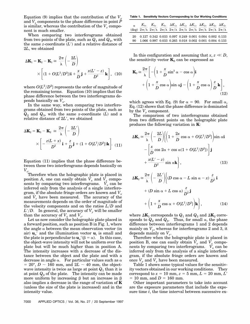
Table 1 shows some typical values for the sensitiv-ity vectors obtained in our working conditions. Theycorrespond to x 5 10 mm, z 5 5 mm, L 5 20 mm, L95 10 mm, and D 5 160 mm.

Other important parameters to take into accountare the exposure parameters that include the expo-sure time t, the time interval between successive ex-

Table 1. Sensitivity Vectors Corresponding to Our Working Conditions

a~deg!

K0x

2pyl

K0y

2pyl

K0z

2pyl

DK1x

2pyl

DK1y

2pyl

DK1z

2pyl

DK2x

2pyl

DK2y

2pyl

DK2z

2pyl

20 0.127 0.342 0.033 0.097 0.249 0.001 0.004 0.002 0.13390 1.066 0.997 0.033 0.265 0.018 0.002 0.001 0.004 0.133

posures DT, the number of exposures N, and thepreexposure time t9. The first three parameters aredetermined in the same way as in PIV17 by the max-imum flow velocity and the desired spatial resolutionof the measurements. The preexposure time is an-other degree of freedom used in HI to adjust the laserintensity to the holographic plate sensitivity.

The time interval DT is determined by the spatialresolution, which means that the number of interfer-ence fringes that can be well resolved on the inter-ferogram is limited. From Eq. ~3!, it can be seen thatthe number of interference fringes on the flow fieldincreases with DT, thus decreasing its spacing.Therefore there is a limit on DT such that

DT , ~2pmmax!y~K z Vmax!, (15)

where mmax is the factor limiting the spatial resolu-tion of the fringes. In addition, as in PIV, there canbe a loss of correlation ~implying a reduction on thefringe visibility! if the particles leave the illuminatedplane during the time interval DT. Thus the illumi-nated plane should have a width Dy such that

Dy . VyDT. (16)

The exposure time t is controllable only when ashuttered continuous beam is being used. There aretwo requirements for t:

~a! The energy should be adequate. In recording ahologram, the energy required Eopt should be suchthat it produces an optical density D 5 0.6 that cor-responds to the linear region of amplitude transmit-tance. If we take the energy of exposure E to belarger than half of Eopt, we get a lower limit for t:

t . Eopty2I, (17)

where I represents the total laser intensity.~b! The effects of time-average holography should

be negligible. From Eq. ~6! and a fringe visibilityabove 0.64, sinc2~K z Vmaxty2! . 0.64, we obtain anupper limit for t:

t , py~K z Vmax!. (18)

This condition can be rewritten, using inequality ~15!,as

t , DTy~2mmax!. (19)

The effect of the number of exposures N is, as inPIV, double. On the one hand, it increases the totalenergy on the plate, which permits either the reduc-tion of the exposure time t or the use of lower-intensity beams. On the other hand, it producesinterference fringes with brighter and sharper max-ima that are easier to detect. This is so because thefunction that locally relates the interferogram inten-sity with the phase changes with N. This effect isnot important in PIV, where only the maxima areneeded to determine the periodicity and orientationof Young’s fringes. However, in HI it is often re-quired to determine the phase in points other than

the fringe maxima. In this case, N 5 2 is the onlyvalue that allows this analysis.

The total amount of energy on the holographicplate can be increased by preexposing the plate for acertain time t9. The purpose of this preexposure is tomake the total energy on the plate lay on the linearregion on the amplitude transmission curve. In thatregion, the response of the plate to small changes inexposure is maximum. In this case, exposure E onthe plate will be

E 5 t9Ir 1 NtI, (20)

where Ir is the intensity of the reference beam and Iis the total intensity ~reference and object beams!.

Taking into account the recommended values forDT @see Eq. ~15!#, it can be shown that the maximumdisplacements, along the direction of K, dmax, allow-able in HI are such that

dmax , mmaxlysin a. (21)

For some typical values such as mmax 5 5 and a 520°, we obtain dmax ; 10 mm. This means that thedisplacements for HI should be approximately 50times smaller than for PIV. For small a, as we havesaid, the interferogram is more sensitive to the out-of-plane velocity component, which means that HIallows the measurement of out-of-plane velocitiesthat are approximately 50 times smaller than thein-plane velocities measured with PIV.

4. Experimental Setup

The technique described here has been demonstratedin a Rayleigh–Benard convective flow set up in a cellwhose dimensions are Lx 5 25 mm, Ly 5 25 mm, andLz 5 12.3 mm. A detailed description of a similarcell was given in a previous paper,20 where some PIVexperiments were carried out. We point out herethat the cell is filled with silicone oil in which 1.1-mmlatex particles are suspended at a concentration ofapproximately 1 order of magnitude higher than inour previously reported PIV experiments.20

The recording setup used for our experiments isshown in Fig. 2. An argon laser with an output of200 mW at a wavelength of 514.5 nm in air is used asa coherent light source. The laser beam is shapedinto a sheet of light that illuminates the convectiveflow. We formed this light sheet using the sameoptical arrangement ~a 43 microscope objective L1and an 86-mm focal-length cylindrical lens Lc! asused in previous PIV experiments.17 We diverted15% of the laser beam by a beam splitter ~BS! to forma clean collimated beam by means of a spatial filterand a convergent lens L2. We recorded on a holo-graphic plate the light scattered by the tracers usingthis collimated beam as the reference beam. Theholographic plate was placed perpendicular to thedirection that formed an angle of 20° with the illumi-nation direction ~equivalent to position B in Fig. 1!.The low power of the laser prevented us from usingother positions ~such as position A in Fig. 1! for theplate. The distance from the plate to the flow was


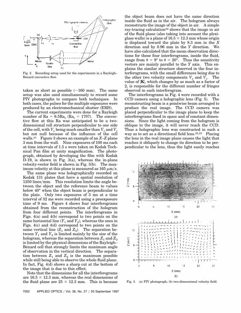
taken as short as possible ~;160 mm!. The samesetup was also used simultaneously to record somePIV photographs to compare both techniques. Inboth cases, the pulses for the multiple exposures wereproduced by an electromechanical shutter ~EMS!.

The current experiments were done for a Rayleighnumber of Ra 5 6.5Rac ~Rac 5 1707!. The convec-tive flow at this Ra was anticipated to be a two-dimensional roll structure perpendicular to one sideof the cell, with Vy being much smaller than Vx and Vzbut not null because of the influence of the cellwalls.21 Figure 3 shows an example of an X–Z plane3 mm from the wall. Nine exposures of 100 ms eachat time intervals of 1.5 s were taken on Kodak Tech-nical Pan film at unity magnification. The photo-graph, obtained by developing the film with KodakD-19, is shown in Fig. 3~a!, whereas the in-planevelocity-vector field is shown in Fig. 3~b!. The max-imum velocity at this plane is measured as 165 mmys.

The same plane was holographically recorded onKodak 131 plates that have a spatial resolution of1250 linesymm. This resolution limits the angle be-tween the object and the reference beam to valuesbelow 40° when the object beam is perpendicular tothe plate. Only two exposures of 3 ms at a timeinterval of 32 ms were recorded using a preexposuretime of 9 ms. Figure 4 shows four interferogramsobtained from the reconstruction of the hologramfrom four different points. The interferograms inFigs. 4~a! and 4~b! correspond to two points on thesame horizontal line ~Y1 and Y2!, whereas the ones inFigs. 4~c! and 4~d! correspond to two points on thesame vertical line ~Z1 and Z2!. The separation be-tween Y1 and Y2 is limited mainly by the size of thehologram, whereas the separation between Z1 and Z2is limited by the physical dimensions of the Rayleigh–Benard cell that strongly limits the maximum angleof observation in the vertical direction. The separa-tion between Z1 and Z2 is the maximum possiblewhile still being able to observe the whole fluid plane.In fact, Fig. 4~d! shows a sharp cut at the bottom ofthe image that is due to this effect.

Note that the dimensions for all the interferogramsare 16.5 3 12.3 mm, whereas the real dimensions ofthe fluid plane are 25 3 12.3 mm. This is because

Fig. 2. Recording setup used for the experiments in a Rayleigh–Benard convective flow.


the object beam does not have the same directioninside the fluid as in the air. The hologram alwaysreconstructs the image of the object in air. A simpleray-tracing calculation22 shows that the image in airof the fluid plane ~also taking into account the plexi-glass walls! is a plane of 16.5 3 12.3 mm whose originis displaced toward the plate by 8.3 mm in the Xdirection and by 0.96 mm in the Y direction. Wehave also calculated that the mean observation direc-tions for these four interferograms, inside the fluid,range from u 5 9° to u 5 20°. Thus the sensitivityvectors are mainly parallel to the Y axis. This ex-plains the similar structure observed in the four in-terferograms, with the small differences being due tothe other two velocity components Vx and Vz. Thevalue of uKu, which changes by as much as a factor of2, is responsible for the different number of fringesobserved in each interferogram.

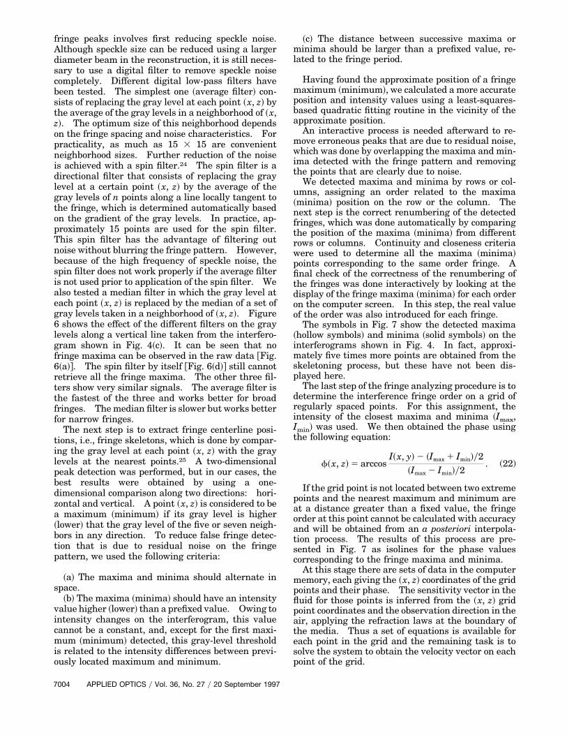
The interferograms in Fig. 4 were recorded with aCCD camera using a holographic lens ~Fig. 5!. Thereconstructing beam is a pointwise beam arranged toproduce the real image. The CCD camera wasplaced perpendicular to the image plane to keep theinterferograms fixed in space and of constant dimen-sions. Since the light coming from the hologram isoblique to the image, it will never reach the CCD.Thus a holographic lens was constructed in such away as to act as a directional field lens.22,23 Placingthe lens in the real image plane causes the light thatreaches it obliquely to change its direction to be per-pendicular to the lens, thus the light easily reaches

Fig. 3. ~a! PIV photograph; ~b! two-dimensional velocity field.

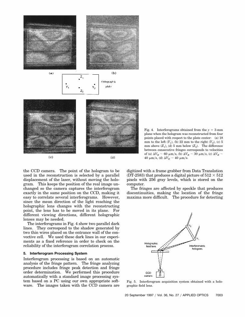
Fig. 4. Interferograms obtained from the y 5 3-mmplane when the hologram was reconstructed from fourpoints placed with respect to the plate center: ~a! 18mm to the left ~Y1!, ~b! 22 mm to the right ~Y2!, ~c! 5mm above ~Z1!, ~d! 5 mm below ~Z2!. The differencebetween consecutive fringes corresponds to velocitiesof ~a! DVK ; 60 mmys, ~b! DVK ; 30 mmys, ~c! DVK ;40 mmys, ~d! DVK ; 40 mmys.

the CCD camera. The point of the hologram to beused in the reconstruction is selected by a paralleldisplacement of the laser, without moving the holo-gram. This keeps the position of the real image un-changed so the camera captures the interferogramexactly in the same position on the CCD, making iteasy to correlate several interferograms. However,since the mean direction of the light reaching theholographic lens changes with the reconstructingpoint, the lens has to be moved in its plane. Fordifferent viewing directions, different holographiclenses may be needed.

The interferograms in Fig. 4 show two parallel darklines. They correspond to the shadow generated bytwo thin wires placed on the entrance wall of the con-vective cell. We used these dark lines in our experi-ments as a fixed reference in order to check on thereliability of the interferogram correlation process.

5. Interferogram Processing System

Interferogram processing is based on an automaticanalysis of the fringe pattern. The fringe analyzingprocedure includes fringe peak detection and fringeorder determination. We performed this procedureautomatically with a standard image processing sys-tem based on a PC using our own appropriate soft-ware. The images taken with the CCD camera are

digitized with a frame grabber from Data Translation~DT-2583! that produces a digital picture of 512 3 512pixels with 256 gray levels, which is stored on thecomputer.

The fringes are affected by speckle that producesdiscontinuities, making the location of the fringemaxima more difficult. The procedure for detecting

Fig. 5. Interferogram acquisition system obtained with a holo-graphic field lens.


fringe peaks involves first reducing speckle noise.Although speckle size can be reduced using a largerdiameter beam in the reconstruction, it is still neces-sary to use a digital filter to remove speckle noisecompletely. Different digital low-pass filters havebeen tested. The simplest one ~average filter! con-sists of replacing the gray level at each point ~x, z! bythe average of the gray levels in a neighborhood of ~x,z!. The optimum size of this neighborhood dependson the fringe spacing and noise characteristics. Forpracticality, as much as 15 3 15 are convenientneighborhood sizes. Further reduction of the noiseis achieved with a spin filter.24 The spin filter is adirectional filter that consists of replacing the graylevel at a certain point ~x, z! by the average of thegray levels of n points along a line locally tangent tothe fringe, which is determined automatically basedon the gradient of the gray levels. In practice, ap-proximately 15 points are used for the spin filter.This spin filter has the advantage of filtering outnoise without blurring the fringe pattern. However,because of the high frequency of speckle noise, thespin filter does not work properly if the average filteris not used prior to application of the spin filter. Wealso tested a median filter in which the gray level ateach point ~x, z! is replaced by the median of a set ofgray levels taken in a neighborhood of ~x, z!. Figure6 shows the effect of the different filters on the graylevels along a vertical line taken from the interfero-gram shown in Fig. 4~c!. It can be seen that nofringe maxima can be observed in the raw data @Fig.6~a!#. The spin filter by itself @Fig. 6~d!# still cannotretrieve all the fringe maxima. The other three fil-ters show very similar signals. The average filter isthe fastest of the three and works better for broadfringes. The median filter is slower but works betterfor narrow fringes.

The next step is to extract fringe centerline posi-tions, i.e., fringe skeletons, which is done by compar-ing the gray level at each point ~x, z! with the graylevels at the nearest points.25 A two-dimensionalpeak detection was performed, but in our cases, thebest results were obtained by using a one-dimensional comparison along two directions: hori-zontal and vertical. A point ~x, z! is considered to bea maximum ~minimum! if its gray level is higher~lower! that the gray level of the five or seven neigh-bors in any direction. To reduce false fringe detec-tion that is due to residual noise on the fringepattern, we used the following criteria:

~a! The maxima and minima should alternate inspace.

~b! The maxima ~minima! should have an intensityvalue higher ~lower! than a prefixed value. Owing tointensity changes on the interferogram, this valuecannot be a constant, and, except for the first maxi-mum ~minimum! detected, this gray-level thresholdis related to the intensity differences between previ-ously located maximum and minimum.


~c! The distance between successive maxima orminima should be larger than a prefixed value, re-lated to the fringe period.

Having found the approximate position of a fringemaximum ~minimum!, we calculated a more accurateposition and intensity values using a least-squares-based quadratic fitting routine in the vicinity of theapproximate position.

An interactive process is needed afterward to re-move erroneous peaks that are due to residual noise,which was done by overlapping the maxima and min-ima detected with the fringe pattern and removingthe points that are clearly due to noise.

We detected maxima and minima by rows or col-umns, assigning an order related to the maxima~minima! position on the row or the column. Thenext step is the correct renumbering of the detectedfringes, which was done automatically by comparingthe position of the maxima ~minima! from differentrows or columns. Continuity and closeness criteriawere used to determine all the maxima ~minima!points corresponding to the same order fringe. Afinal check of the correctness of the renumbering ofthe fringes was done interactively by looking at thedisplay of the fringe maxima ~minima! for each orderon the computer screen. In this step, the real valueof the order was also introduced for each fringe.

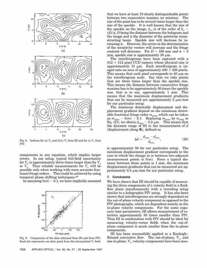
The symbols in Fig. 7 show the detected maxima~hollow symbols! and minima ~solid symbols! on theinterferograms shown in Fig. 4. In fact, approxi-mately five times more points are obtained from theskeletoning process, but these have not been dis-played here.

The last step of the fringe analyzing procedure is todetermine the interference fringe order on a grid ofregularly spaced points. For this assignment, theintensity of the closest maxima and minima ~Imax,Imin! was used. We then obtained the phase usingthe following equation:

f~x, z! 5 arccosI~x, y! 2 ~Imax 1 Imin!y2

~Imax 2 Imin!y2. (22)

If the grid point is not located between two extremepoints and the nearest maximum and minimum areat a distance greater than a fixed value, the fringeorder at this point cannot be calculated with accuracyand will be obtained from an a posteriori interpola-tion process. The results of this process are pre-sented in Fig. 7 as isolines for the phase valuescorresponding to the fringe maxima and minima.

At this stage there are sets of data in the computermemory, each giving the ~x, z! coordinates of the gridpoints and their phase. The sensitivity vector in thefluid for those points is inferred from the ~x, z! gridpoint coordinates and the observation direction in theair, applying the refraction laws at the boundary ofthe media. Thus a set of equations is available foreach point in the grid and the remaining task is tosolve the system to obtain the velocity vector on eachpoint of the grid.

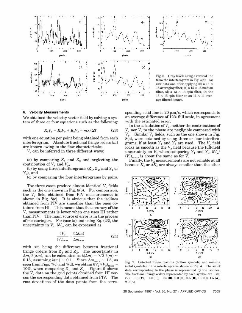
Fig. 6. Gray levels along a vertical linefrom the interferogram in Fig. 4~c!: ~a!raw data and after applying ~b! a 15 315 averaging filter, ~c! a 15 3 15 medianfilter, ~d! a 13 3 13 spin filter, ~e! the15 3 15 spin filter on an 11 3 11 aver-age filtered image.

6. Velocity Measurements

We obtained the velocity-vector field by solving a sys-tem of three or four equations such as the following:

KxVx 1 KyVy 1 KzVz 5 mlyDT (23)

with one equation per point being obtained from eachinterferogram. Absolute fractional fringe orders ~m!are known owing to the flow characteristics.

Vz can be inferred in three different ways:

~a! by comparing Z1 and Z2 and neglecting thecontribution of Vx and Vy,

~b! by using three interferograms ~Z1, Z2, and Y1 orY2!, and

~c! by comparing the four interferograms by pairs.

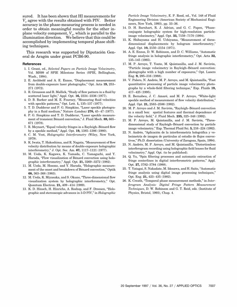
The three cases produce almost identical Vz fieldssuch as the one shown in Fig. 8~b!. For comparison,the Vz field obtained from PIV measurements isshown in Fig. 8~c!. It is obvious that the isolinesobtained from PIV are smoother than the ones ob-tained from HI. This means that the accuracy of theVz measurements is lower when one uses HI ratherthan PIV. The main source of error is in the processof measuring m. For case ~a! and using Eq. ~23!, theuncertainty in Vz, dVz, can be expressed as

dVz

~Vz!max5

dD~m!

Dmmax(24)

with Dm being the difference between fractionalfringe orders from Z1 and Z2. The uncertainty inDm, d~Dm!, can be calculated as d~Dm! 5 =2 d~m! ;0.15, assuming d~m! ; 0.1. Since Dmmax ; 1.5, asseen from Figs. 7~c! and 7~d!, we obtain dVzy~Vz!max ;10%, when comparing Z1 and Z2. Figure 9 showsthe Vz data on the grid points obtained from HI ver-sus the corresponding data obtained from PIV. Therms deviations of the data points from the corre-

sponding solid line is 20 mmys, which corresponds toan average difference of 12% full scale, in agreementwith the estimated error.

In the calculation of Vy, neither the contributions ofVx nor Vz to the phase are negligible compared withVy. Similar Vy fields, such as the one shown in Fig.8~a!, were obtained by using three or four interfero-grams, if at least Y1 and Y2 are used. The Vy fieldlooks as smooth as the Vz field because the full-fielduncertainty on Vy when comparing Y1 and Y2, dVyy~Vz!max, is about the same as for Vz.

Finally, the Vx measurements are not reliable at allbecause Kx or DKx are always smaller than the other

Fig. 7. Detected fringe maxima ~hollow symbols! and minima~solid symbols! in the interferograms shown in Fig. 4. The set ofdata corresponding to the phase is represented by the isolines.The fractional fringe orders represented by each symbol are 22.0~ƒ!, 21.5 ~�!, 21.0 ~h!, 20.5 ~■!, 0.0 ~3!, 0.5 ~F!, 1.0 ~E!, 1.5 ~Œ!,2.0 ~‚!.


components in any equation, which implies largererrors. In our setup, typical full-field uncertaintyfor Vx is approximately three times larger than for Vyor Vz. Thus reliable measurements for Vx will bepossible only when working with more accurate frac-tional fringe orders. This could be achieved by usingtemporal phase shifting techniques.26

In assuming d~m! ; 0.1, we have implicitly assumed

Fig. 8. Isolines for ~a! Vy and ~b!~c! Vz from HI and for ~c! Vz fromPIV.

Fig. 9. Comparison of the data obtained from HI and from PIV.Each dot represents one data point from the interpolated Vz field.


that we have at least 10 clearly distinguishable pointsbetween two consecutive maxima ~or minima!. Thesize of the point has to be several times larger than thesize of the speckle. It is well known that the size ofthe speckle on the image, bs, is of the order of bs ;lDyf, D being the distance between the hologram andthe image and f the diameter of the pointwise recon-structing beam. Speckle size will decrease by in-creasing f. However, the errors in the determinationof the sensitivity vectors will increase and the fringecontrast will decrease. For D 5 160 mm and f 5 3mm, speckle size is approximately 30 mm.

The interferograms have been captured with a512 3 512 pixel CCD camera whose physical size isapproximately 15 mm. Each interferogram is im-aged onto an area of approximately 430 3 320 pixels.This means that each pixel corresponds to 40 mm onthe interferogram scale. Say that we take pointsthat are three times larger than the speckle size.This means the distance between consecutive fringemaxima has to be approximately 30 times the specklesize, that is to say, approximately 1 mm. Thismeans that the maximum displacement gradientsthat can be measured are approximately 2 mmymmfor our particular setup.

The minimum detectable displacement and dis-placement gradient depend on the minimum detect-able fractional fringe order mmin, which can be takenas mmin ; d~m! ; 0.1. Replacing mmax by mmin inEq. ~21!, we obtain dmin ; 0.2 mm. This means thatthe dynamic range of HI in the measurement of d~displacement along K!, defined as

Dd 5dmax 2 dmin

dmin, (25)

is approximately 50 for our particular setup. Theminimum displacement gradient corresponds to thecase in which the change in m between two adjacentmeasurement points is d~m!. Since a typical dis-tance between these points is 1 mm, the minimumdisplacement gradients that can be measured are ap-proximately 0.2 mmymm for our particular setup.

7. Conclusions

We have shown that HI should be capable of measur-ing the three components of a velocity field in a fluid-flow plane simultaneously with a recording setupsimilar to a holographic PIV setup. It has also beenshown that interferograms are strongly dependent onthe out-of-plane velocity component as opposed to thePIV photographs, which are dependent mainly on thein-plane velocity components. For the same expo-sure time parameters, HI allows measurement of ve-locities approximately 50 times smaller than PIV.Thus HI in combination with PIV should be ideal formeasuring velocity-vector fields when the out-of-plane component is much smaller than the in-planecomponents.

HI has been successfully applied to a Rayleigh–Benard convective flow. The out-of-plane, Vy, andone in-plane, Vz, velocity components have been mea-

sured. It has been shown that HI measurements forVz agree with the results obtained with PIV. Betteraccuracy in the phase-measuring process is needed inorder to obtain meaningful results for the other in-plane velocity component, Vx, which is parallel to theillumination direction. We believe that this could beaccomplished by implementing temporal phase shift-ing techniques.

This research was supported by Diputacion Gen-eral de Aragon under grant PCB6-90.

References1. I. Grant, ed., Selected Papers on Particle Image Velocimetry,

Vol. MS99 of SPIE Milestone Series ~SPIE, Bellingham,Wash., 1994!.

2. E. Archbold and A. E. Ennos, “Displacement measurementfrom double-exposure laser photographs,” Opt. Acta 19, 253–271 ~1972!.

3. R. Grousson and R. Mallick, “Study of flow pattern in a fluid byscattered laser light,” Appl. Opt. 16, 2334–2336 ~1977!.

4. D. B. Barker and M. E. Fourney, “Measuring fluid velocitieswith speckle patterns,” Opt. Lett. 1, 135–137 ~1977!.

5. T. D. Dudderar and P. G. Simpkins, “Laser speckle photogra-phy in a fluid medium,” Nature ~London! 270, 45–47 ~1977!.

6. P. G. Simpkins and T. D. Dudderar, “Laser speckle measure-ment of transient Benard convection,” J. Fluid Mech. 89, 665–671 ~1978!.

7. R. Meynart, “Equal velocity fringes in a Rayleigh–Benard flowby a speckle method,” Appl. Opt. 19, 1385–1386 ~1980!.

8. C. M. Vest, Holographic Interferometry ~Wiley, New York,1979!.

9. K. Iwata, T. Hakoshima, and R. Nagata, “Measurement of flowvelocity distribution by means of double-exposure holographicinterferometry,” J. Opt. Soc. Am. 67, 1117–1121 ~1977!.

10. M. Ueda, K. Kagawa, K. Yamada, C. Yamaguchi, and Y.Harada, “Flow visualization of Benard convection using holo-graphic interferometry,” Appl. Opt. 21, 3269–3272 ~1982!.

11. M. Ueda, M. Hosono, and Y. Harada, “Holographic measure-ment of the onset and breakdown of Benard convection,” Optik68, 363–368 ~1983!.

12. M. Ueda, K. Miyasaka, and S. Okuno, “Three-dimensional flowvisualization system by holographic interferometry,” Opt.Quantum Electron. 21, 409–414 ~1989!.

13. K. D. Hinsch, H. Hinrichs, A. Roshop, and F. Dreesen, “Holo-graphic and stereoscopic advances in 3-D PIV,” in Holographic

2

Particle Image Velocimetry, E. P. Rood, ed., Vol. 148 of FluidEngineering Division ~American Society of Mechanical Engi-neers, New York, 1993!, pp. 33–36.

14. D. H. Barnhart, R. J. Adrian, and G. C. Papen, “Phase-conjugate holographic system for high-resolution particle-image velocimetry,” Appl. Opt. 33, 7159–7170 ~1994!.

15. K. Shibayama and H. Uchiyama, “Measurement of three-dimensional displacements by hologram interferometry,”Appl. Opt. 10, 2150–2154 ~1971!.

16. A. E. Ennos, D. W. Robinson, and D. C. Williams, “Automaticfringe analysis in holographic interferometry,” Opt. Acta 32,135–145 ~1985!.

17. M. P. Arroyo, T. Yonte, M. Quintanilla, and J. M. Saviron,“Particle image velocimetry in Rayleigh–Benard convection:photographs with a high number of exposures,” Opt. LasersEng. 9, 295–316 ~1988!.

18. V. Palero, N. Andres, M. P. Arroyo, and M. Quintanilla, “Fastquantitative processing of particle image velocimetry photo-graphs by a whole-field filtering technique,” Exp. Fluids 19,417–425 ~1995!.

19. E. Bernabeu, J. C. Amare, and M. P. Arroyo, “White-lightspeckle method of measurement of flow velocity distribution,”Appl. Opt. 21, 2583–2586 ~1982!.

20. M. P. Arroyo and J. M. Saviron, “Rayleigh–Benard convectionin a small box: spatial features and thermal dependence ofthe velocity field,” J. Fluid Mech. 235, 325–348 ~1992!.

21. M. P. Arroyo, M. Quintanilla, and J. M. Saviron, “Three-dimensional study of Rayleigh–Benard convection by particleimage velocimetry,” Exp. Thermal Fluid Sci. 5, 216–224 ~1992!.

22. N. Andres, “Aplicacion de la interferometrıa holografica y ve-locimetrıa de imagen de partıculas al estudio de flujos convec-tivos,” Ph.D. dissertation ~University of Zaragoza, Spain, 1994!.

23. N. Andres, M. P. Arroyo, and M. Quintanilla, “Distortionlessinterferogram recording using holographic field lenses for fluidvelocimetry,” Appl. Opt. ~to be published!.

24. Q. Yu, “Spin filtering processes and automatic extraction offringe centerlines in digital interferometric patterns,” Appl.Opt. 27, 3782–3784 ~1988!.

25. T. Yatagai, S. Nakadate, M. Idesawa, and H. Saito, “Automaticfringe analysis using digital image processing techniques,”Opt. Eng. 21, 423–435 ~1982!.

26. K. Creath, “Temporal phase measurement methods,” in Inter-ferogram Analysis: Digital Fringe Pattern MeasurementTechniques, D. W. Robinson and G. T. Reid, eds. ~Institute ofPhysics, Bristol, 1993!, Chap. 4.


velocity measurements in a convective flow by holographic interferometry

Documents