vc.03 gradient vectors, level curves, maximums/minimums/saddle points
TRANSCRIPT
VC.03
Gradient Vectors, Level Curves, Maximums/Minimums/Saddle Points
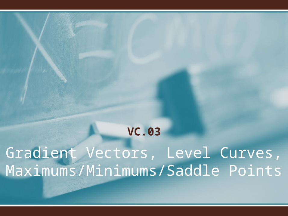
Example 1: The Gradient Vector
2 dfLet f(x) x . Then 2x.Thiscanbethought of asavector that
dxtells you the direction of greatest increase on the curve. The magnitude
of the vector tells you how steep the increase.
Let's try a few
dfx-valuesin :
dx
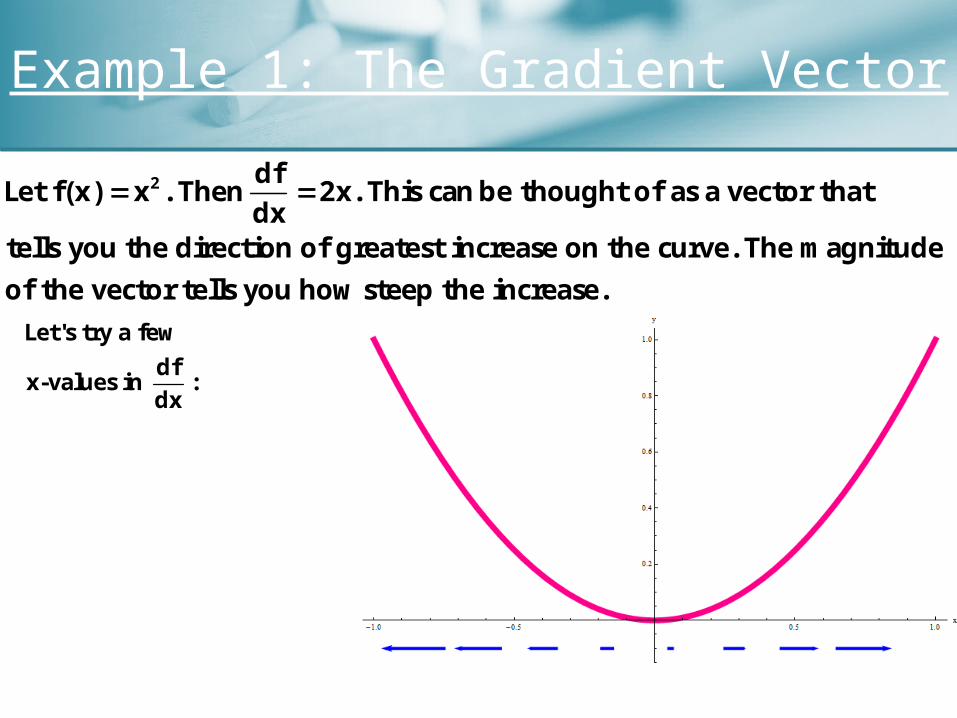
Example 1: The Gradient Vector
We can put the tails of our vectors on the curve itself
to get picture that's a little easier to work with:What do you notice about the magnitude of the gradient vector at x=0?
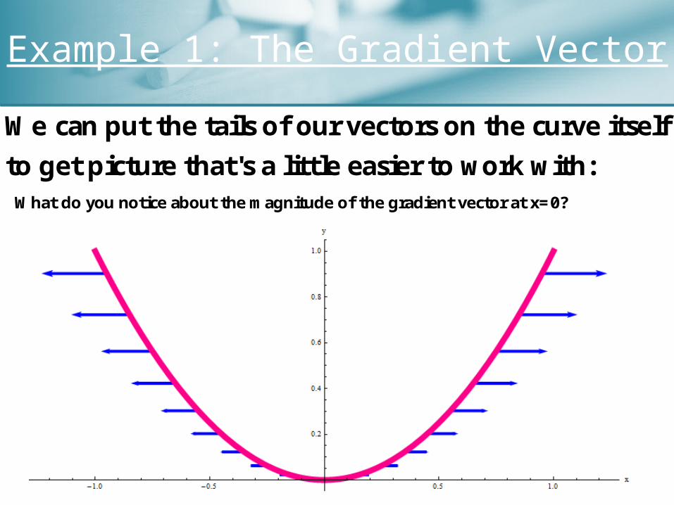
Example 2: The Gradient Vector
We can try again with f(x) sin(x) :
3What do you notice about the magnitude of the gradient vector at x and x ?
2 2
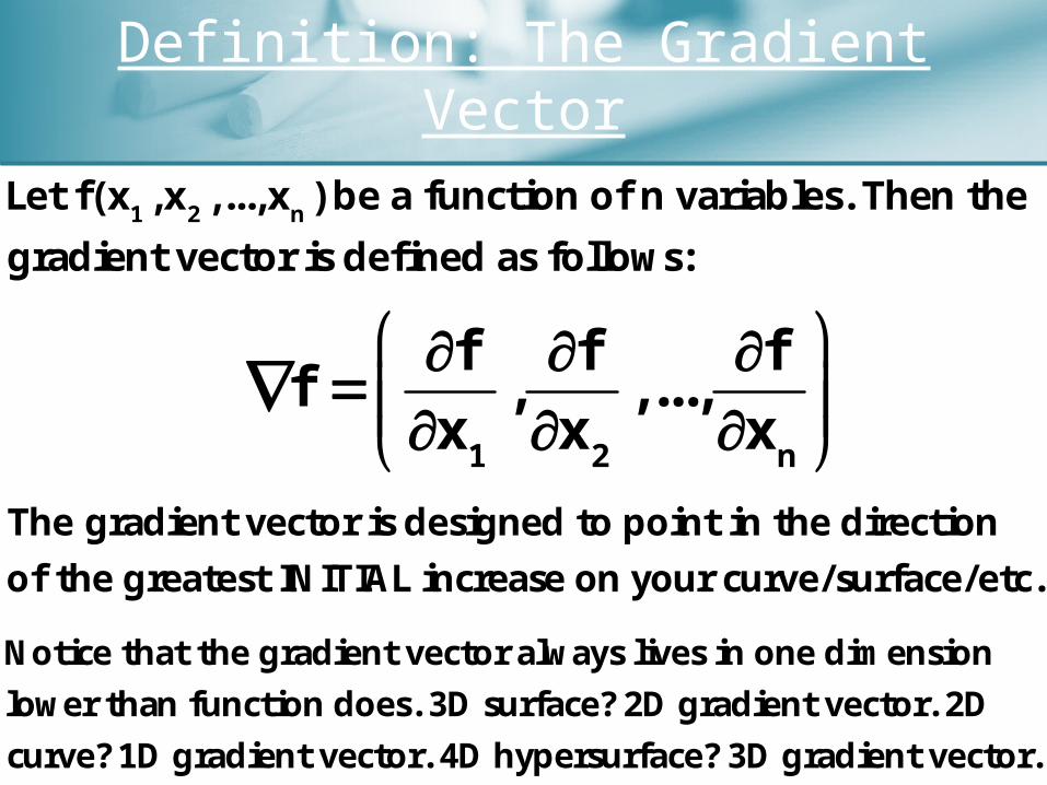
Definition: The Gradient Vector
1 2 nLet f(x ,x ,...,x )be a function of n variables. Then the
gradient vector is defined as follows:
1 2 n
ff ff , ,...,
x x x
The gradient vector is designed to point in the direction
of the greatest INITIAL increase on your curve/surface/etc.
Notice that the gradient vector always lives in one dimension
lower than function does. 3D surface?2D gradient vector. 2D
curve?1D gradient vector. 4D hypersurface? 3D gradient vector.
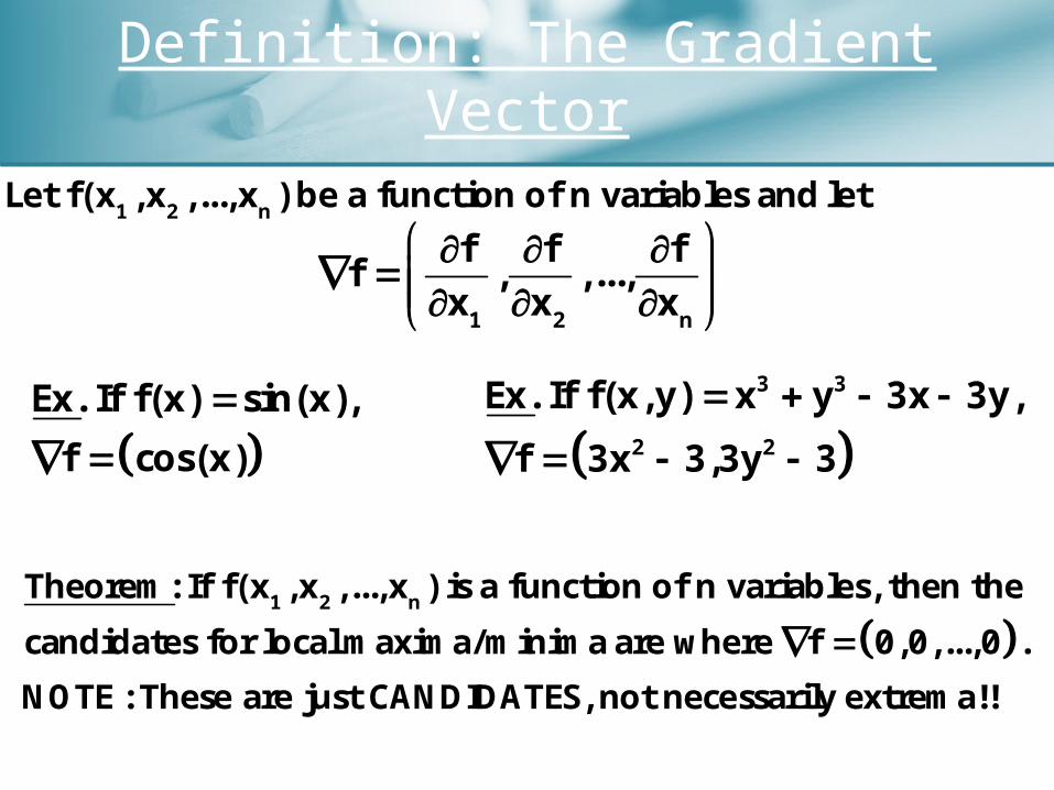
Definition: The Gradient Vector
1 2 nLet f(x ,x ,...,x )be a function of n variablesandlet
1 2 n
ff ff , ,...,
x x x
Ex. Iff (x) sin(x),
f cos(x)
3 3
2 2
Ex. Iff (x,y) x y 3x 3y,
f 3x 3,3y 3
1 2 nTheorem:Iff (x ,x ,...,x ) isa function of n variables, then the
candidatesfor localmaxima/minimaarewhere f 0,0,...,0 .
NOTE:These are just CANDIDATES, not necessarily extrema!!
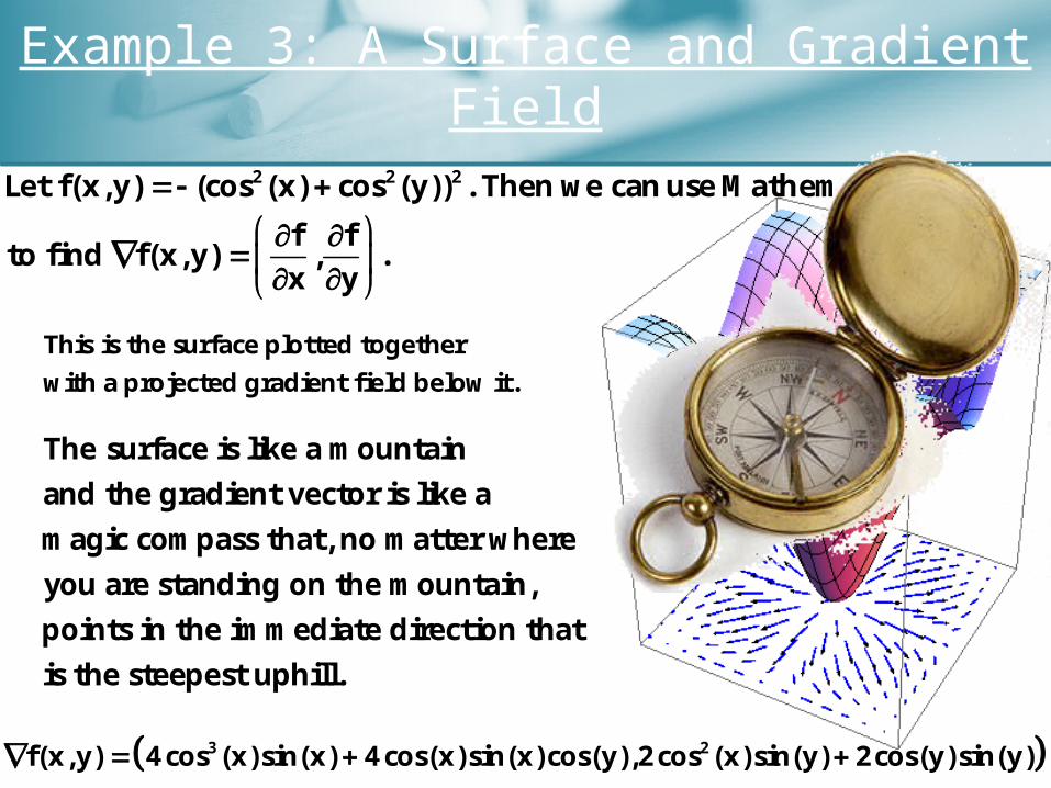
Example 3: A Surface and Gradient Field
2 2 2Let f(x,y) (cos (x) cos (y)) . ThenwecanuseMathematica
ffto find f(x,y) , .
x y
This is the surface plotted together
with a projected gradient field below it.
3 2f(x,y) 4cos (x)sin(x) 4cos(x)sin(x)cos(y),2cos (x)sin(y) 2cos(y)sin(y)
The surface is like a mountain
and the gradient vector is like a
magiccompass that, no matter where
you are standing on the mountain,
points in the immediate direction that
is the steepest uphill.
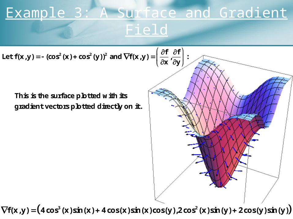
Example 3: A Surface and Gradient Field
2 2 2 ffLet f(x,y) (cos (x) cos (y)) and f(x,y) , :
x y
This is the surface plotted withits
gradient vectors plotted directly on it.
3 2f(x,y) 4cos (x)sin(x) 4cos(x)sin(x)cos(y),2cos (x)sin(y) 2cos(y)sin(y)
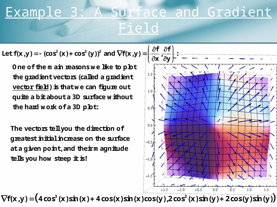
Example 3: A Surface and Gradient Field
2 2 2 ffLet f(x,y) (cos (x) cos (y)) and f(x,y) , :
x y
One of the main reasons we like to plot
the gradient vectors (called a gradient
vector field) is that we can figure out
quite a bit about a 3D surface without
the hard work of a 3D plot:
3 2f(x,y) 4cos (x)sin(x) 4cos(x)sin(x)cos(y),2cos (x)sin(y) 2cos(y)sin(y)
The vectors tell you the direction of
greatest initial increase on the surface
at a given point, and their magnitude
tellsyou how steep it is!
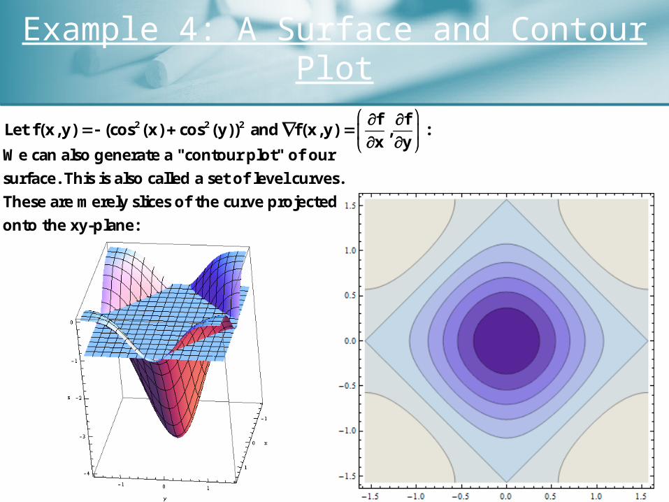
Example 4: A Surface and Contour Plot
2 2 2 ffLet f(x,y) (cos (x) cos (y)) and f(x,y) , :
x y
Wecan also generate a "contour plot" of our
surface. This is also called a set of level curves.
These are merely slices of the curve projected
onto the xy-plane:
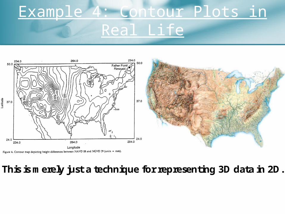
Example 4: Contour Plots in Real Life
This is merely just a technique for representing 3D data in 2D.
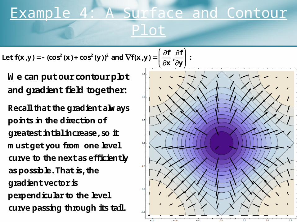
Example 4: A Surface and Contour Plot
Wecan put our contour plot
and gradient field together:
2 2 2 ffLet f(x,y) (cos (x) cos (y)) and f(x,y) , :
x y
Recall that the gradient always
points in the direction of
greatest intial increase, so it
must get you from one level
curve to the next as efficiently
as possible. That is, the
gradient vector is
perpendicular to the level
curve passing through its tail.
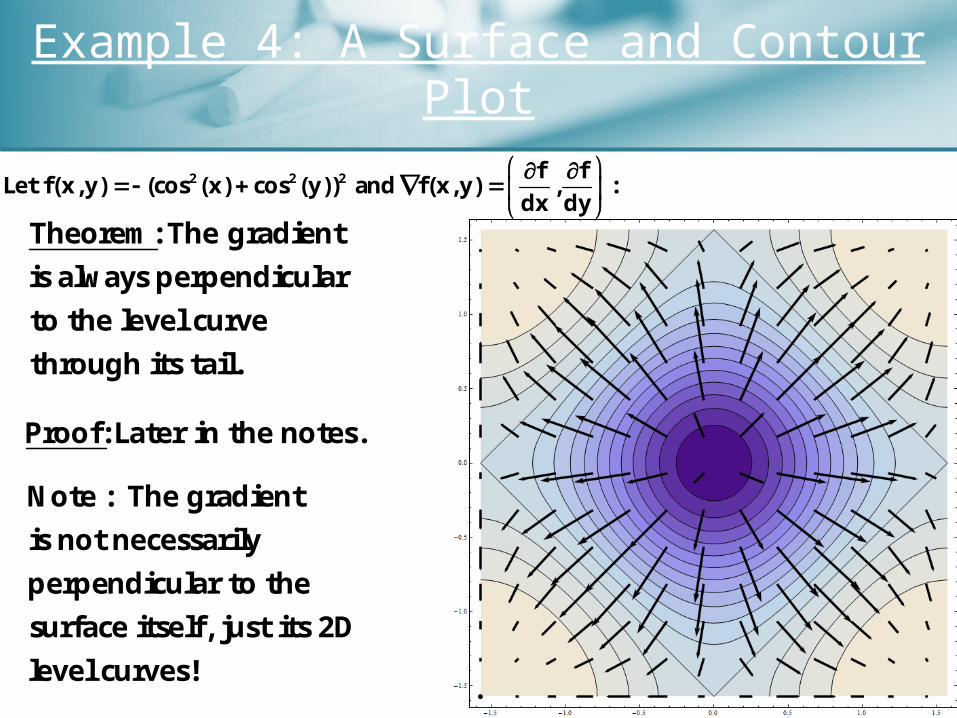
Example 4: A Surface and Contour Plot
2 2 2 ff
Let f(x,y) (cos (x) cos (y)) and f(x,y) , :dx dy
Theorem:The gradient
isalways perpendicular
to the level curve
through its tail.
Note: The gradient
is not necessarily
perpendicular to the
surface itself, just its 2D
level curves!
Proof:Later in the notes.
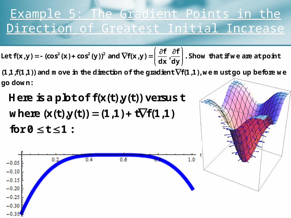
Example 5: The Gradient Points in the Direction of Greatest Initial Increase
2 2 2 ffLet f(x,y) (cos (x) cos (y)) and f(x,y) , . Show that if we are at point
dx dy
(1,1,f(1,1)) and move in the direction of the gradient f(1,1),wemust go up before we
go down:
Here isa plot off (x(t),y(t)) versust
where(x(t),y(t)) (1,1) t f(1,1)
for 0 t 1:
Example 6: A Path Along our Surface
2 2 22 (x(t),y(t)) cos (1 t),Let andlet .
Finall f(x
f(x,y) (c
(t),y(t)
sin(2t
y,plot ,a path on
os (x) cos
the sur
(y))
)
)
face.
The surface is a like a mountain
and the path is a hiking trail on
that mountain!
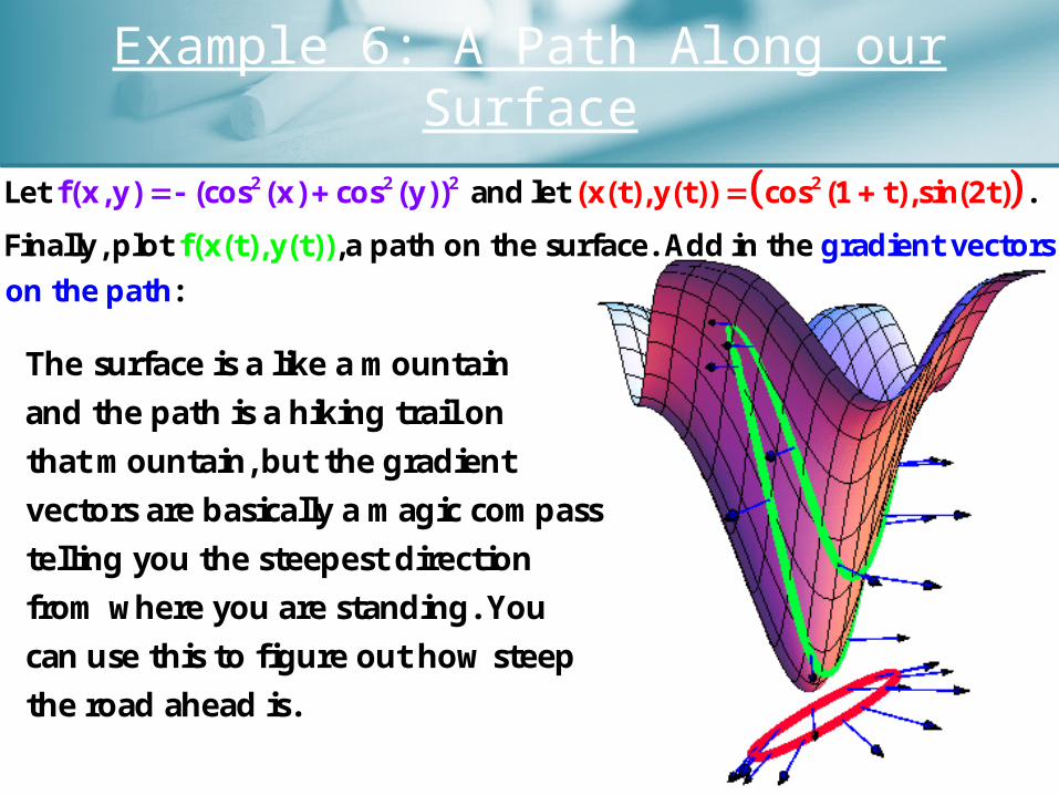
Example 6: A Path Along our Surface
22 2 2Let andlet .
Finally,pl f(x(t),y(t))ot ,a path on the
(x(t),y(t)) cos (1 t),
surface. Addinthegr
sin(2t)
adient
f(x,y
vecto
) (cos
rs
on
(x)
the
cos
p
(y))
ath:
The surface is a like a mountain
and the path is a hiking trail on
that mountain,but thegradient
vectors are basically a magic compass
telling you the steepest direction
from where you are standing. You
can use this to figure out how steep
the road ahead is.
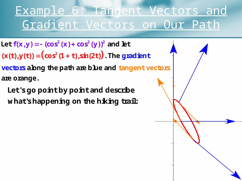
Example 6: Tangent Vectors and Gradient Vectors on Our Path
2 2
2
2Let andlet
. T gradient
vectors
( he
alo
x(t),y
ngthep
f(x
ath
(t)) cos (1 t),sin
arebluea t
,y) (cos (x) co
angent vector
s
s
(y))
nd
areora
(2t)
nge.
Let'sgo point by point and describe
what'shappening on the hiking trail:
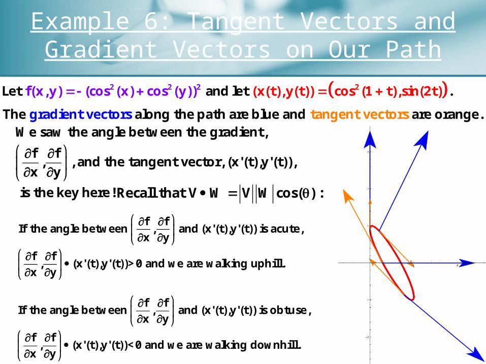
Example 6: Tangent Vectors and Gradient Vectors on Our Path
2 2 22Let andlet .
T gradient vectors
(
he alo
x(t),y
ngthep
f(x
ath
(t)) cos (1 t),sin
arebluea t
,y) (cos (x) co
angent vector
s
s
(y))
nd areora
(2t)
nge.Wesaw theanglebetweenthegradient,
ff, ,andthe tangent vector,(x'(t),y'(t)),
x y
isthekeyhere!
Recall that V W V W cos( ) :
ffIf theanglebetween , and(x'(t),y'(t)) isacute,
x y
ff, (x'(t),y'(t))>0andwe arewalking uphill.
x y
ffIf theanglebetween , and(x'(t),y'(t)) isobtuse,
x y
ff, (x'(t),y'(t))<0andwe arewalking downhill.
x y
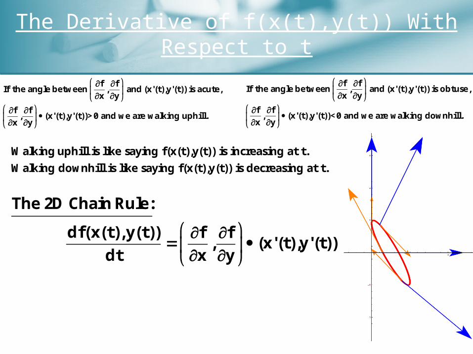
The Derivative of f(x(t),y(t)) With Respect to t
ffIf theanglebetween , and(x'(t),y'(t)) isacute,
x y
ff, (x'(t),y'(t))>0andwe arewalking uphill.
x y
ffIf theanglebetween , and(x'(t),y'(t)) isobtuse,
x y
ff, (x'(t),y'(t))<0andwe arewalking downhill.
x y
Walkinguphill is like saying f(x(t),y(t)) is increasing at t.
Walking downhill is like saying f(x(t),y(t)) is decreasing at t.
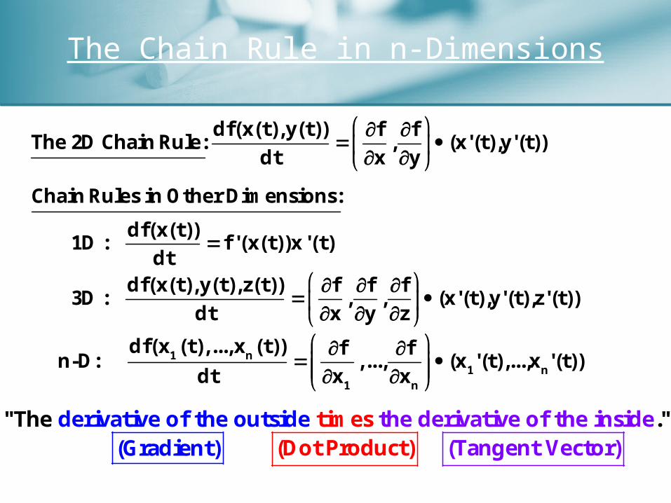
The2D ChainRule:
df(x(t),y(t)) ff, (x'(t),y'(t))
dt x y
The Chain Rule in n-Dimensions
df(x(t),y(t)) ffThe2D ChainRule: , (x'(t),y'(t))
dt x y
1 n1 n
1 n
ChainRulesinOtherDimensions:
df(x(t))1D: f'(x(t))x'(t)
dtdf(x(t),y(t),z(t)) ff f
3D: , , (x'(t),y'(t),z'(t))dt x y z
df(x (t),...,x (t)) ffn-D: ,..., (x '(t),...,x '(t))
dt x x
times"The the dederivative of rivative of t the o he insu itside de."(Gradient) (DotProduct) (Tangent Vector)
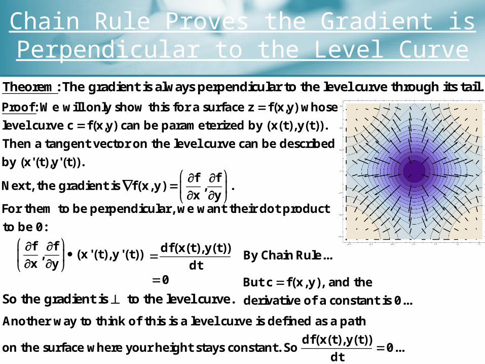
Chain Rule Proves the Gradient is Perpendicular to the Level Curve
Theorem:The gradient isalways perpendicular to the level curvethrough its tail.
Proof:We will only show this for a surface z f(x,y) whose
level curvec f(x,y) can be parameterized by(x(t),y(t)).
Then atangent vector on the level curvecan be described
by (x'(t),y'(t)).ff
Next, thegradient is f(x,y) , .x y
For themtobeperpendicular,we want their dot product
to be 0:
ff, (x'(t),y'(t))
x y
df(x(t),y(t))dt
0 But c f(x,y), and the
derivative of a constant is 0...
By ChainRule...
Another way to think of this is a level curve is defined as a path
df(x(t),y(t))on the surface where your height stays constant. So 0...
dt
So the gradient is to the level curve.
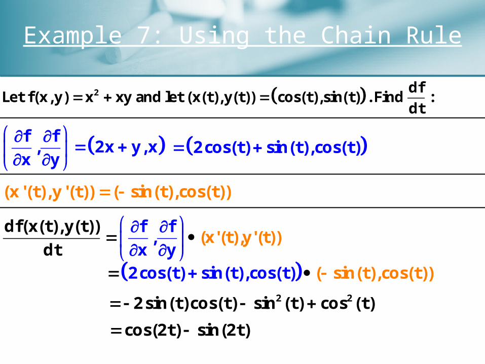
Example 7: Using the Chain Rule
2 dfLet f(x,y) x xy andlet(x(t),y(t)) cos(t),sin(t) .Find :
dt
ff,
xdf(x(t),y(t)
y)
dt(x'(t),y'(t))
ff, 2x y,x
x y
2cos(t) sin(t),cos(t)
(x'(t),y'(t)) ( sin(t),cos(t))
2cos(t) sin(t),cos( ( sin(t),co () ))t s t 2 22sin(t)cos(t) sin (t) cos (t)
cos(2t) sin(2t)
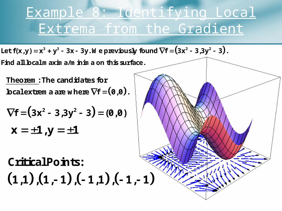
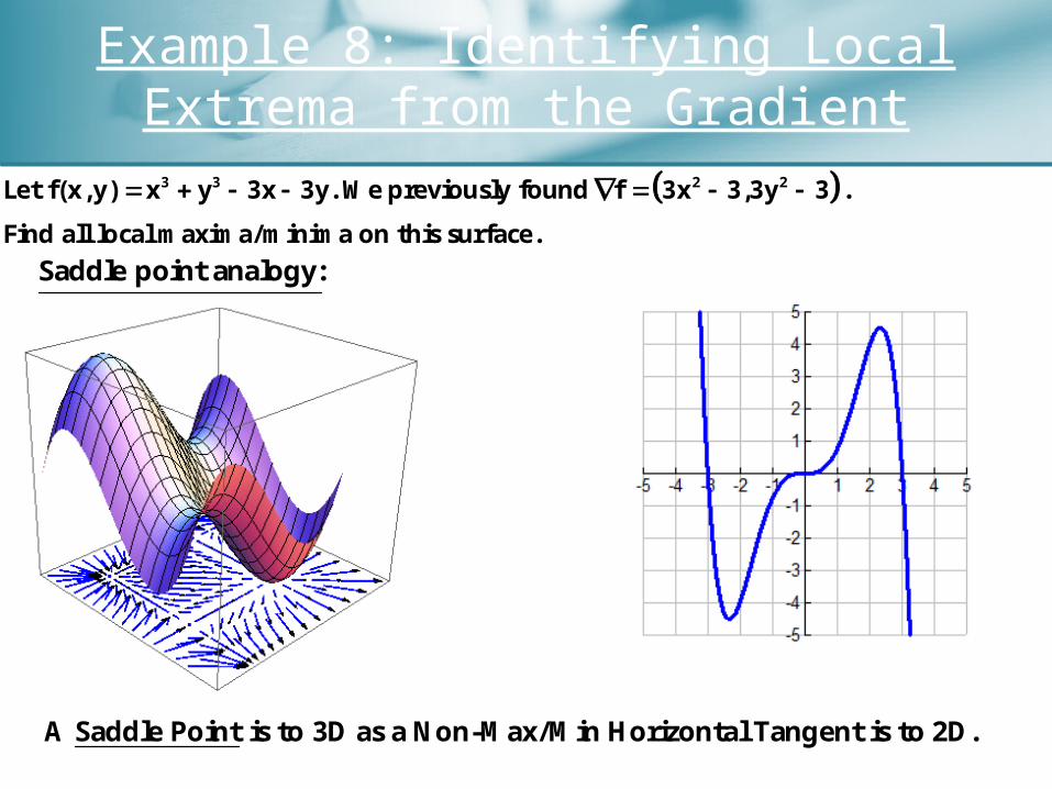
Example 8: Identifying Local Extrema from the Gradient
3 3 2 2Let f(x,y) x y 3x 3y. Wepreviously found f 3x 3,3y 3 .
Find all local maxima/minima on this surface.
Theorem:Thecandidatesfor
local extremaarewhere f 0,0 .
2 2f 3x 3,3y 3 (0,0)
x 1,y 1
CriticalPoints:
1,1 , 1, 1 , 1,1 , 1, 1
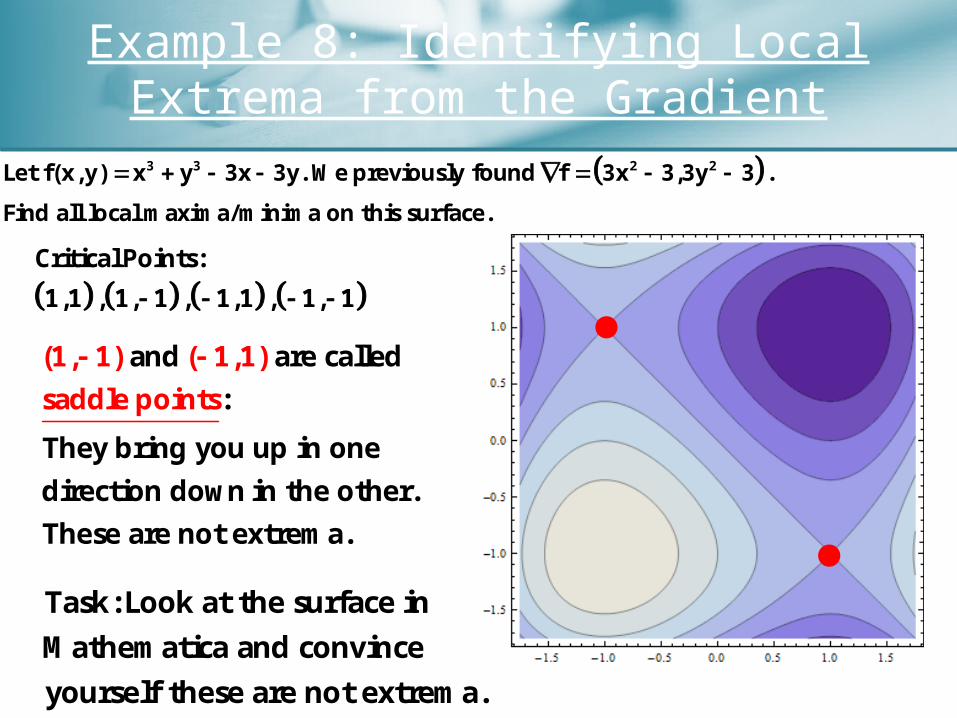
Example 8: Identifying Local Extrema from the Gradient
3 3 2 2Let f(x,y) x y 3x 3y. Wepreviously found f 3x 3,3y 3 .
Find all local maxima/minima on this surface.
and arecalled
:
They bring you up in one
direction downin the other.
T
(1, 1) ( 1,1)
saddlep
hese are not extr
oints
ema.
Task:Look at the surface in
Mathematica and convince
yourself these are not extrema.
CriticalPoints:
1,1 , 1, 1 , 1,1 , 1, 1
Example 8: Identifying Local Extrema from the Gradient
3 3 2 2Let f(x,y) x y 3x 3y. Wepreviously found f 3x 3,3y 3 .
Find all local maxima/minima on this surface.
Saddle point analogy:
A Saddle Point is to 3D as a Non-Max/Min Horizontal Tangent isto 2D.
Example 8: Identifying Local Extrema from the Gradient
3 3 2 2Let f(x,y) x y 3x 3y. Wepreviously found f 3x 3,3y 3 .
Find all local maxima/minima on this surface.
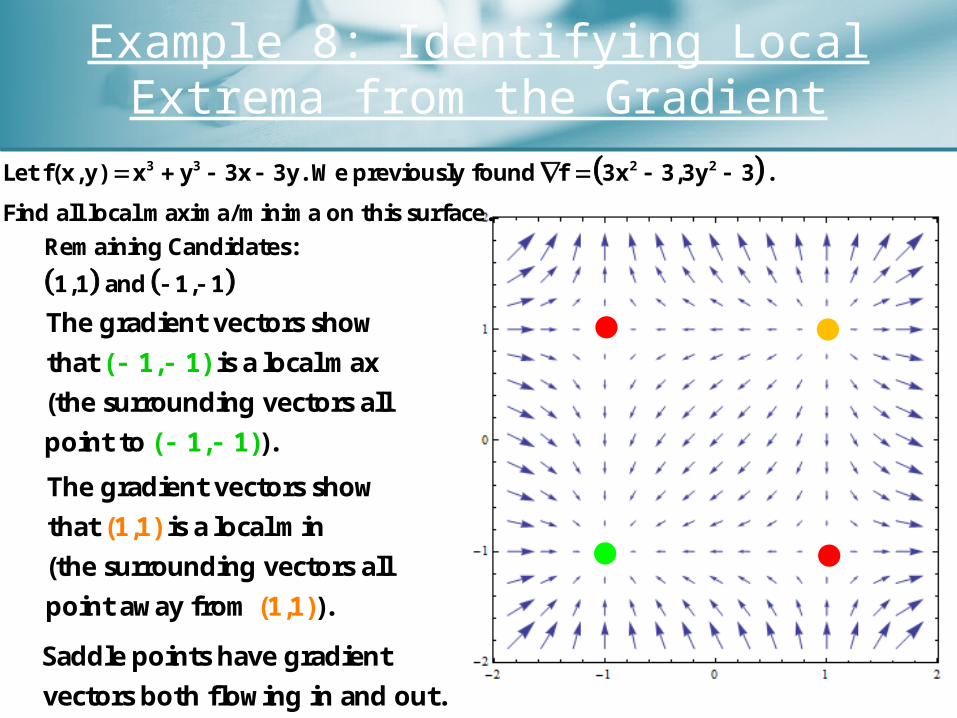
Thegradient vectorsshow
that isalocalmax
(thesurrounding vectors all
point
( 1, 1)
( 1to , 1)).
RemainingCandidates:
1,1 and 1, 1
Thegradient vectorsshow
that isalocalmin
(thesurrounding vectors all
point away fr
(1,1)
(om 1,1)).
Saddlepoints have gradient
vectors both flowing in and out.
Example 8: Identifying Local Extrema from the Gradient
3 3 2 2Let f(x,y) x y 3x 3y. Wepreviously found f 3x 3,3y 3 .
Find all local maxima/minima on this surface.
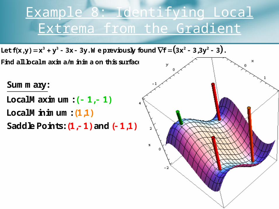
Summary:
LocalMaximum:
LocalMinimum:
SaddlePoi (1,
( 1
1
,
)
1)
nts: a (
(1,1)
nd 1,1)
Example 9: Another Visit to Our Surface
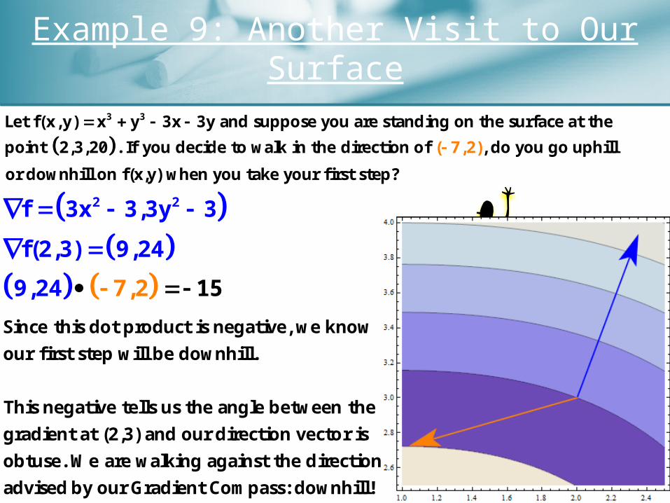
3 3Let f(x,y) x y 3x 3y and suppose you are standing on the surface at the
point 2,3,20 . If you decide to walk in the direction of , do you go uphill
or downhill on f(x,y) when you take your first st
(
e
7,2)
p?
2 2f 3x 3,3y 3
f(2,3) 9,24
7,9, 2 124 5
Since this dot product is negative, we know
our first step will be downhill.
This negativetells us the angle between the
gradient at (2,3)and our direction vector is
obtuse. We are walking against the direction
advisedby our Gradient Compass: downhill!
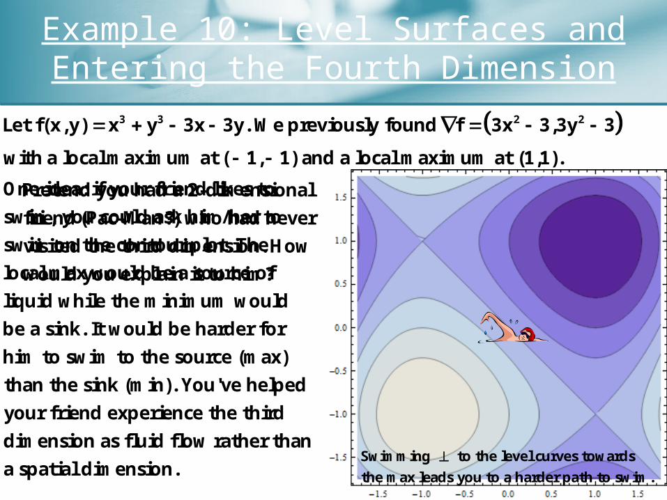
Example 10: Level Surfaces and Entering the Fourth Dimension
3 3 2 2Let f(x,y) x y 3x 3y. Wepreviously found f 3x 3,3y 3
witha localmaximumat( 1, 1)and a local maximum at (1,1).
Pretend you had a 2-dimensional
friend(Pac-Man?) who had never
visited the third dimension. How
would you explain it to him?
Oneidea: if your friend likes to
swim, you could ask him/her to
swim on the contour plot. The
local max would be a source of
liquid while the minimum would
be a sink. It would be harder for
him to swim to the source (max)
than the sink (min). You've helped
your friend experience the third
dimension as fluid flow rather than
a spatial dimension.Swimming to the level curves towards
the max leads you to a harder path to swim.
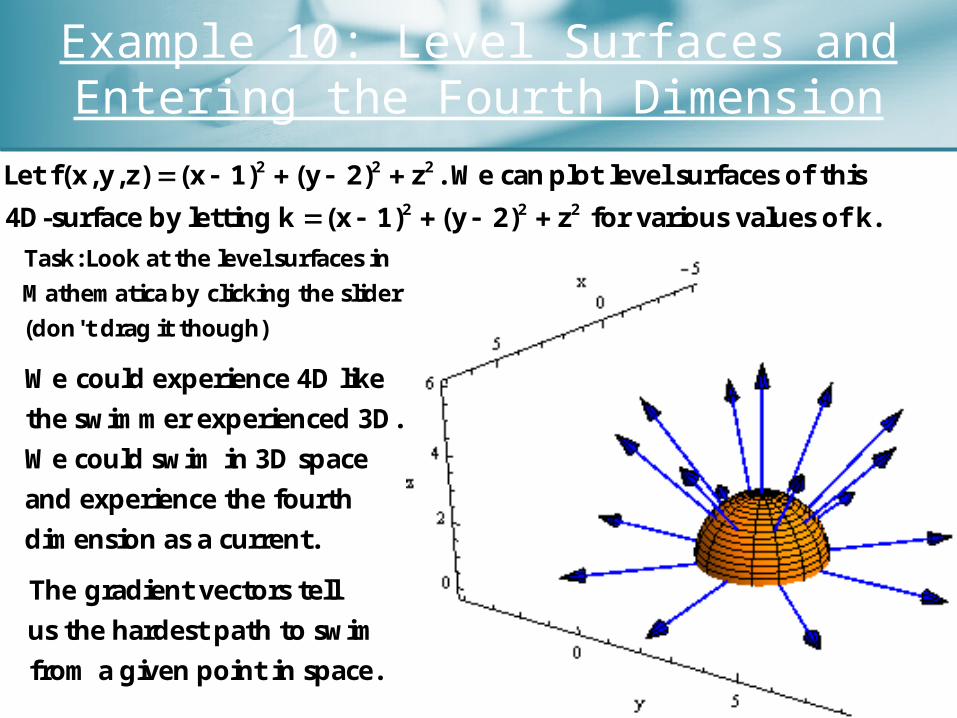
Example 10: Level Surfaces and Entering the Fourth Dimension
2 2 2
2 2 2
Let f(x,y,z) (x 1) (y 2) z . Wecanplot level surfaces of this
4D-surface by letting k (x 1) (y 2) z for variousvalues of k.
Task:Look at the level surfacesin
Mathematicaby clicking the slider
(don't dragit though)
We could experience 4D like
theswimmer experienced 3D.
We could swim in 3D space
and experience the fourth
dimension as a current.
The gradient vectors tell
us the hardest path to swim
from a given point in space.
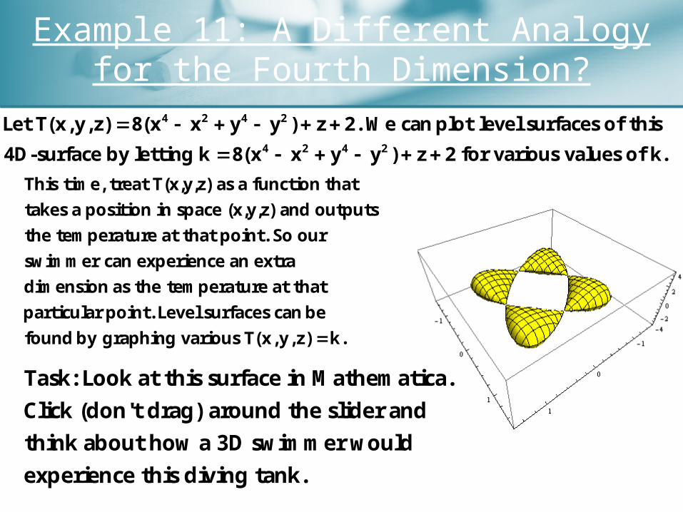
Example 11: A Different Analogy for the Fourth Dimension?
4 2 4 2
4 2 4 2
Let T(x,y,z) z 2. Wecanplot level surfaces of this
4
8(x x y y )
8D-surface by letting k z 2for variousvalues of k(x x y y ) .
This time, treat T(x,y,z) as a functionthat
takes a position in space (x,y,z) and outputs
the temperature at that point. So our
swimmer can experience an extra
dimensionasthe temperatureat that
particular point.Level surfacescanbe
foundby graphing various T(x,y,z) k.
Task: Look at this surface in Mathematica.
Click (don't drag) around the slider and
think about how a 3D swimmer would
experience this diving tank.
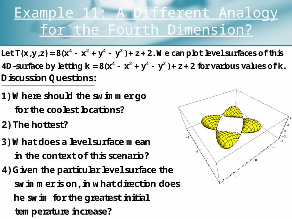
Example 11: A Different Analogy for the Fourth Dimension?
4 2 4 2
4 2 4 2
Let T(x,y,z) z 2. Wecanplot level surfaces of this
4
8(x x y y )
8D-surface by letting k z 2for variousvalues of k(x x y y ) .
1) Where should the swimmer go
for the coolest locations?
DiscussionQuestions:
2) The hottest?
3) What does a level surface mean
in the context of this scenario?
4)Giventhe particular level surface the
swimmer is on, in what direction does
he swim for the greatest initial
temperature increase?
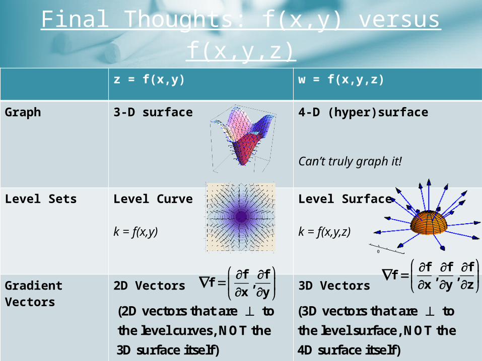
z = f(x,y) w = f(x,y,z)
Graph 3-D surface 4-D (hyper)surface
Can’t truly graph it!
Level Sets Level Curve
k = f(x,y)
Level Surface
k = f(x,y,z)
Gradient Vectors
2D Vectors 3D Vectors
fff ,
x y
ff ff , ,
x y z
(2D vectors that are to
thelevel curves, NOT the
3D surfaceitself)
(3D vectors that are to
thelevel surface, NOT the
4D surfaceitself)
Final Thoughts: f(x,y) versus f(x,y,z)