This article was downloaded by: [Manukau Institute of Technology]On: 04 October 2014, At: 15:26Publisher: Taylor & FrancisInforma Ltd Registered in England and Wales Registered Number: 1072954 Registered office: MortimerHouse, 37-41 Mortimer Street, London W1T 3JH, UK

Journal of Nonlinear Mathematical PhysicsPublication details, including instructions for authors and subscription information:http://www.tandfonline.com/loi/tnmp20

Variational derivation of the Camassa-Holm shallowwater equationDelia Ionescu-Kruse aa Institute of Mathematics of the Romanian Academy , P.O. Box 1–764, RO–014700,Bucharest , Romania E-mail:Published online: 21 Jan 2013.

To cite this article: Delia Ionescu-Kruse (2007) Variational derivation of the Camassa-Holm shallow water equation,Journal of Nonlinear Mathematical Physics, 14:3, 311-320, DOI: 10.2991/jnmp.2007.14.3.1

To link to this article: http://dx.doi.org/10.2991/jnmp.2007.14.3.1

PLEASE SCROLL DOWN FOR ARTICLE

Taylor & Francis makes every effort to ensure the accuracy of all the information (the “Content”) containedin the publications on our platform. However, Taylor & Francis, our agents, and our licensors make norepresentations or warranties whatsoever as to the accuracy, completeness, or suitability for any purpose ofthe Content. Any opinions and views expressed in this publication are the opinions and views of the authors,and are not the views of or endorsed by Taylor & Francis. The accuracy of the Content should not be reliedupon and should be independently verified with primary sources of information. Taylor and Francis shallnot be liable for any losses, actions, claims, proceedings, demands, costs, expenses, damages, and otherliabilities whatsoever or howsoever caused arising directly or indirectly in connection with, in relation to orarising out of the use of the Content.

This article may be used for research, teaching, and private study purposes. Any substantial or systematicreproduction, redistribution, reselling, loan, sub-licensing, systematic supply, or distribution in anyform to anyone is expressly forbidden. Terms & Conditions of access and use can be found at http://www.tandfonline.com/page/terms-and-conditions

Journal of Nonlinear Mathematical Physics Volume 14, Number 3 (2007), 311–320 Letter

Variational derivation of the Camassa-Holm

shallow water equation

Delia IONESCU-KRUSE

Institute of Mathematics of the Romanian Academy,P.O. Box 1-764, RO-014700, Bucharest, RomaniaE-mail: Delia.Ionescu@imar.ro

Received February 7, 2007; Accepted in Revised Form March 17, 2007

Abstract

We describe the physical hypothesis in which an approximate model of water waves isobtained. For an irrotational unidirectional shallow water flow, we derive the Camassa-Holm equation by a variational approach in the Lagrangian formalism.

1 Introduction

The Camassa-Holm equation reads

Ut + 2κUx + 3UUx − Utxx = 2UxUxx + UUxxx (1.1)

with x ∈ R, t ∈ R, U(x, t) ∈ R. Subscripts here, and later, denote partial derivatives.The constant κ is related to the critical shallow water speed. For κ=0 the equation (1.1)possesses peaked soliton solutions ([3]). The physical derivation of (1.1) as a model forthe evolution of a shallow water layer under the influence of gravity, is due to Camassaand Holm [3]. See also Refs. [5], [16] for alternative derivations within the shallow waterregime. In [19] it was shown that the equation (1.1) describes a geodesic flow on the onedimensional central extension of the group of diffeomorphisms of the circle (for the caseκ=0, a geodesic flow on the diffeomorphism group of the circle, see also [9]). It shouldbe mentioned that, prior to Camassa and Holm, Fokas and Fuchssteiner [12] obtainedformally, by the method of recursion operators in the context of hereditary symmetries,families of integrable equations containing (1.1). These equations are bi-Hamiltoniangeneralizations of the KdV equation and possess infinitely many conserved quantities ininvolution ([12]). In order to see how the equation (1.1) relates with one of equationsin the families introduced in [12], see [14], §2.2. Also, the equation (5.3) in [13] is theequation (1.1) but with errors in the coefficients.

The Camassa-Holm equation attracted a lot of interest, due to its complete integrability[10] (for the periodic case), [8] and the citations therein (for the integrability on the line),the existence of waves of permanent form and of breaking waves [7] and the presence ofpeakon solutions [3] (for a more rigorous study on the peakons see for example [2]). An

Copyright c© 2007 by Delia Ionescu-Kruse

Dow

nloa

ded

by [

Man

ukau

Ins

titut

e of

Tec

hnol

ogy]

at 1

5:26

04

Oct

ober

201

4

312 Delia Ionescu-Kruse

important question to be answered is whether solutions of the water wave problem canreally be approximated by solutions of the Camassa-Holm equation. In [18] it is shown thatsuitable solutions of the water wave problem and solutions of the Camassa-Holm equationstay close together for long times, in the case ǫ = δ2, ǫ being the amplitude parameterand δ the shallowness parameter. In [18] it is also shown that the peakon equation cannotstrictly be derived from the Euler equation and hence it is at most a phenomenologicalmodel.

The present paper is concerned with the physical hypothesis in which an approximatemodel of water waves is obtained, with the derivation of the Camassa-Holm equation bya variational approach in the Lagrangian formalism, and with the role of this equationwithin the shallow water problem.

2 The governing equations for water waves

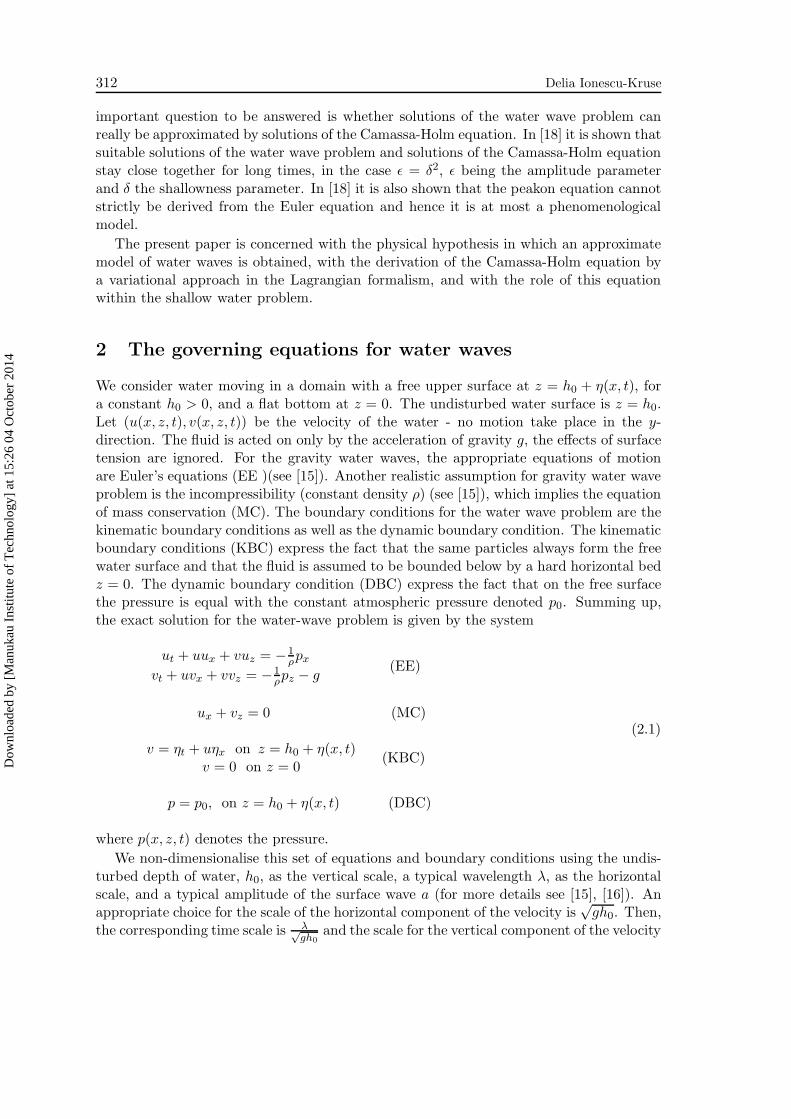
We consider water moving in a domain with a free upper surface at z = h0 + η(x, t), fora constant h0 > 0, and a flat bottom at z = 0. The undisturbed water surface is z = h0.Let (u(x, z, t), v(x, z, t)) be the velocity of the water - no motion take place in the y-direction. The fluid is acted on only by the acceleration of gravity g, the effects of surfacetension are ignored. For the gravity water waves, the appropriate equations of motionare Euler’s equations (EE )(see [15]). Another realistic assumption for gravity water waveproblem is the incompressibility (constant density ρ) (see [15]), which implies the equationof mass conservation (MC). The boundary conditions for the water wave problem are thekinematic boundary conditions as well as the dynamic boundary condition. The kinematicboundary conditions (KBC) express the fact that the same particles always form the freewater surface and that the fluid is assumed to be bounded below by a hard horizontal bedz = 0. The dynamic boundary condition (DBC) express the fact that on the free surfacethe pressure is equal with the constant atmospheric pressure denoted p0. Summing up,the exact solution for the water-wave problem is given by the system

ut + uux + vuz = −1

ρpx

vt + uvx + vvz = −1

ρpz − g

(EE)

ux + vz = 0 (MC)

v = ηt + uηx on z = h0 + η(x, t)v = 0 on z = 0

(KBC)

p = p0, on z = h0 + η(x, t) (DBC)

(2.1)

where p(x, z, t) denotes the pressure.

We non-dimensionalise this set of equations and boundary conditions using the undis-turbed depth of water, h0, as the vertical scale, a typical wavelength λ, as the horizontalscale, and a typical amplitude of the surface wave a (for more details see [15], [16]). Anappropriate choice for the scale of the horizontal component of the velocity is

√gh0. Then,

the corresponding time scale is λ√gh0

and the scale for the vertical component of the velocity

Dow

nloa

ded

by [

Man

ukau

Ins

titut

e of

Tec

hnol

ogy]

at 1

5:26

04

Oct

ober

201

4

Variational derivation of the Camassa-Holm shallow water equation 313

is h0

√gh0

λ. Thus, we define the set of non-dimensional variables

x 7→ λx, z 7→ h0z, η 7→ aη, t 7→ λ√gh0

t,

u 7→ √gh0u, v 7→ h0

√gh0

λv

(2.2)

where, to avoid new notations, we have used the same symbols for the non-dimensionalvariables x, z, η, t, u, v, in the right-hand side. The partial derivatives will be replacedby

ut 7→ gh0

λut, ux 7→

√gh0

λux, uz 7→

√gh0

h0uz,

vt 7→ gh02

λ2 vt, vx 7→ h0

√gh0

λ2 vx, vz 7→√

gh0

λvz,

(2.3)

Let us now define the non-dimensional pressure. If the water would be stationary, that is,u ≡ v ≡ 0, from the first two equations and the last condition with η = 0, of the system(2.1), we get for a non-dimensionalised z, the hydrostatic pressure p0 +ρgh0(1− z). Thus,the non-dimensional pressure is defined by

p 7→ p0 + ρgh0(1 − z) + ρgh0p (2.4)

and

px 7→ ρgh0

λpx, pz 7→ −ρg + ρgpz (2.5)

Taking into account (2.2), (2.3), (2.4), and (2.5), the water-wave problem (2.1) writesin non-dimensional variables, as

ut + uux + vuz = −px

δ2(vt + uvx + vvz) = −pz

ux + vz = 0v = ǫ(ηt + uηx) and p = ǫη on z = 1 + ǫη(x, t)

v = 0 on z = 0

(2.6)

where we have introduced the amplitude parameter ǫ = ah0

and the shallowness parameter

δ = h0

λ. The small-amplitude shallow water is obtained in the limits ǫ → 0, δ → 0. We

observe that, on z = 1 + ǫη, both v and p are proportional to ǫ. This is consistent withthe fact that as ǫ→ 0 we must have v → 0 and p→ 0, and it leads to the following scalingof the non-dimensional variables

p 7→ ǫp, (u, v) 7→ ǫ(u, v) (2.7)

where we avoided again the introduction of a new notation. The problem (2.6) becomes

ut + ǫ(uux + vuz) = −px

δ2[vt + ǫ(uvx + vvz)] = −pz

ux + vz = 0v = ηt + ǫuηx and p = η on z = 1 + ǫη(x, t)

v = 0 on z = 0

(2.8)

Dow

nloa

ded

by [

Man

ukau

Ins

titut

e of

Tec

hnol

ogy]

at 1

5:26

04

Oct

ober

201

4

314 Delia Ionescu-Kruse

Further, the parameter δ can be removed from the system (2.8) (see [16]), this beingequivalent to use only h0 as the length scale of the problem. In order to do this, thenon-dimensional variables x, t and v from (2.2) are replaced by

x 7→√ǫ

δx, t 7→

√ǫ

δt, v 7→ δ√

ǫv (2.9)

Therefore the equations in the system (2.8) are recovered, but with δ2 replaced by ǫ inthe second equation of the system, that is, this equation writes as

ǫ[vt + ǫ(uvx + vvz)] = −pz (2.10)

3 The Camassa-Holm equation

The non-dimensionalisation and scaling presented above will be useful in obtaining ascheme of approximation of the governing water-wave problem (2.1).

In the limit ǫ→ 0, that is for small-amplitude waves, the system (2.8) with the secondequation given by (2.10) becomes

ut + px = 0pz = 0

ux + vz = 0v = ηt and p = η on z = 1

v = 0 on z = 0

(3.1)

From the second equation in (3.1), we get that p does not depend on z. Because p = η(x, t)on z = 1, we have

p = η(x, t) for any 0 ≤ z ≤ 1 (3.2)

Therefore, using the first equation in (3.1), we obtain

u = −∫

ηx(x, t)dt + F(x, z) (3.3)

where F is an arbitrary function. Differentiating (3.3) with respect to x and using thethird equation in (3.1), we get, after an integration against z,

v = z

∫

ηxx(x, t)dt− G(x, z) + G(x, 0) (3.4)

where Gz(x, z) = Fx(x, z) and we have also taken into account the last condition in thesystem (3.1). Making z = 1 in (3.4), and taking into account that v = ηt on z = 1, we getafter a differentiation with respect to t, that η has to satisfy the equation

ηtt − ηxx = 0 (3.5)

The general solution of this equation is η(x, t) = f(x − t) + g(x + t), where f and g aredifferentiable functions. It is convenient first to restrict ourselves to waves which propagatein only one direction, thus, we choose

η(x, t) = f(x− t) (3.6)

Dow

nloa

ded

by [

Man

ukau

Ins

titut

e of

Tec

hnol

ogy]

at 1

5:26

04

Oct

ober

201

4

Variational derivation of the Camassa-Holm shallow water equation 315

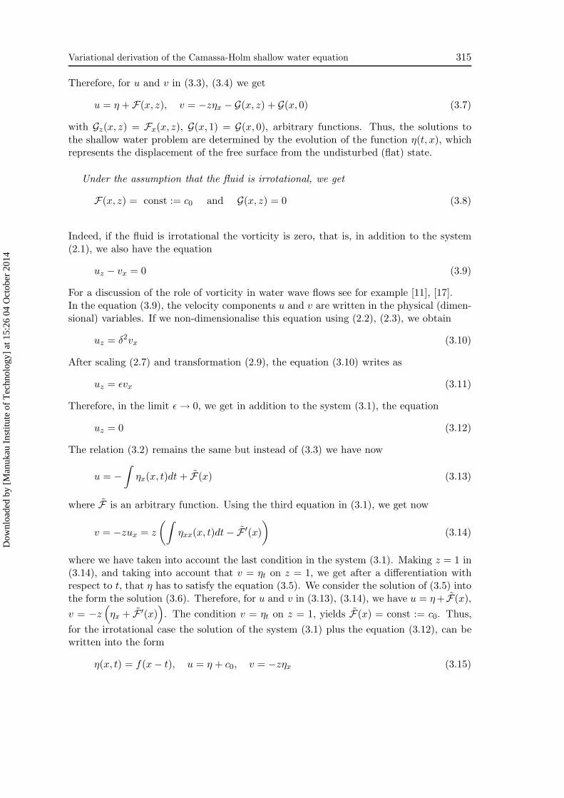
Therefore, for u and v in (3.3), (3.4) we get

u = η + F(x, z), v = −zηx − G(x, z) + G(x, 0) (3.7)

with Gz(x, z) = Fx(x, z), G(x, 1) = G(x, 0), arbitrary functions. Thus, the solutions tothe shallow water problem are determined by the evolution of the function η(t, x), whichrepresents the displacement of the free surface from the undisturbed (flat) state.

Under the assumption that the fluid is irrotational, we get

F(x, z) = const := c0 and G(x, z) = 0 (3.8)

Indeed, if the fluid is irrotational the vorticity is zero, that is, in addition to the system(2.1), we also have the equation

uz − vx = 0 (3.9)

For a discussion of the role of vorticity in water wave flows see for example [11], [17].In the equation (3.9), the velocity components u and v are written in the physical (dimen-sional) variables. If we non-dimensionalise this equation using (2.2), (2.3), we obtain

uz = δ2vx (3.10)

After scaling (2.7) and transformation (2.9), the equation (3.10) writes as

uz = ǫvx (3.11)

Therefore, in the limit ǫ→ 0, we get in addition to the system (3.1), the equation

uz = 0 (3.12)

The relation (3.2) remains the same but instead of (3.3) we have now

u = −∫

ηx(x, t)dt + F(x) (3.13)

where F is an arbitrary function. Using the third equation in (3.1), we get now

v = −zux = z

(∫

ηxx(x, t)dt− F ′(x)

)

(3.14)

where we have taken into account the last condition in the system (3.1). Making z = 1 in(3.14), and taking into account that v = ηt on z = 1, we get after a differentiation withrespect to t, that η has to satisfy the equation (3.5). We consider the solution of (3.5) intothe form the solution (3.6). Therefore, for u and v in (3.13), (3.14), we have u = η+ F(x),

v = −z(

ηx + F ′(x))

. The condition v = ηt on z = 1, yields F(x) = const := c0. Thus,

for the irrotational case the solution of the system (3.1) plus the equation (3.12), can bewritten into the form

η(x, t) = f(x− t), u = η + c0, v = −zηx (3.15)

Dow

nloa

ded

by [

Man

ukau

Ins

titut

e of

Tec

hnol

ogy]

at 1

5:26

04

Oct

ober

201

4

316 Delia Ionescu-Kruse

We underline the fact that in our approximation the vertical velocity component maintainsa dependence on the z-variable. In analyzing the motion of the fluid particles, this meansthat the particles below the surface may perform a vertical motion. This is in agreementwith a recent general result obtained in [6] for the Stokes waves, i.e. particular waves inan irrotational flow which are solutions of the full Euler equations.

By consistently neglecting the ǫ contribution, we will derive using variational methods inthe Lagrangian formalism (see [5]), the equation (1.1) governing unidirectional propagationof shallow water waves.

In the Lagrangian formulation of a fluid, the flow pattern is obtained by describing thepath of each individual water particle. Consider the ambient space M whose points aresupposed to represent the fluid particles at t = 0. A diffeomorphism of M represents therearrangement of the particles with respect to their initial positions. The motion of thefluid is described by a time-dependent family of orientation-preserving diffeomorphismsγ(t, ·) ∈ Diff(M). A point x in M follows the trajectory γ(t, x) through M . For ourproblem, since a particle on the water’s free surface will always stay on the surface anddescribes progressive plane wave (no motion take place in the y direction), we may regardthe motion at that of a one-dimensional membrane. For the one-dimensional periodicmotion, M = S1 the unit circle. We can allow M = R and add the technical assumptionthat the smooth functions defined on R with value in R vanish rapidly at ±∞ togetherwith as many derivatives as necessary (see [4] for a possible choice of weighted Sobolevspaces). In what follows we focus on the latter situation.

For a fluid particle initially located at x, the velocity at time t is γt(t, x), this beingthe material velocity used in the Lagrangian description. The spatial velocity, used in theEulerian description, is the flow velocity w(t,X) = γt(t, x) at the location X = γ(t, x) attime t, that is, w(t, ·) = γt ◦ γ−1. In Lagrangian description, the equation of motion isthe equation satisfied by a critical point of a certain functional (called the action) definedon all paths {γ(t, ·), t ∈ [0, T ]} in Diff(R), having fixed endpoints. Following Arnold’sapproach to Euler equations on diffeomorphism groups ([1]), the action for our problemwill be obtained by transporting the kinetic energy to all tangent spaces of Diff(R) bymeans of right translations. For small surface elevation, the potential energy is negligiblecompared to the kinetic energy. Taking into account (3.15), the kinetic energy on thesurface is

K =1

2

∫ ∞

−∞(u2 + v2)dx =

1

2

∫ ∞

−∞

[

u2 + (1 + ǫη)2u2

x

]

dx ≈ 1

2

∫ ∞

−∞

(

u2 + u2

x

)

dx (3.16)

to the order of our approximation (see [5]). We observe that if we replace the path γ(t, ·)by γ(t, ·) ◦ ψ(·), for a fixed time-independent ψ in Diff(R), then the spatial velocity isunchanged γt ◦γ−1. Transforming K to a right-invariant Lagrangian, the action on a pathγ(t, ·), t ∈ [0, T ], in Diff(R) is

a(γ) =1

2

∫ T

0

∫ ∞

−∞{(γt ◦ γ−1)2 + [∂x(γt ◦ γ−1)]2}dxdt (3.17)

The critical points of the action (3.17) in the space of paths with fixed endpoints, verify

d

dεa(γ + εϕ)

∣

∣

∣

ε=0

= 0, (3.18)

Dow

nloa

ded

by [

Man

ukau

Ins

titut

e of

Tec

hnol

ogy]

at 1

5:26

04

Oct

ober

201

4

Variational derivation of the Camassa-Holm shallow water equation 317

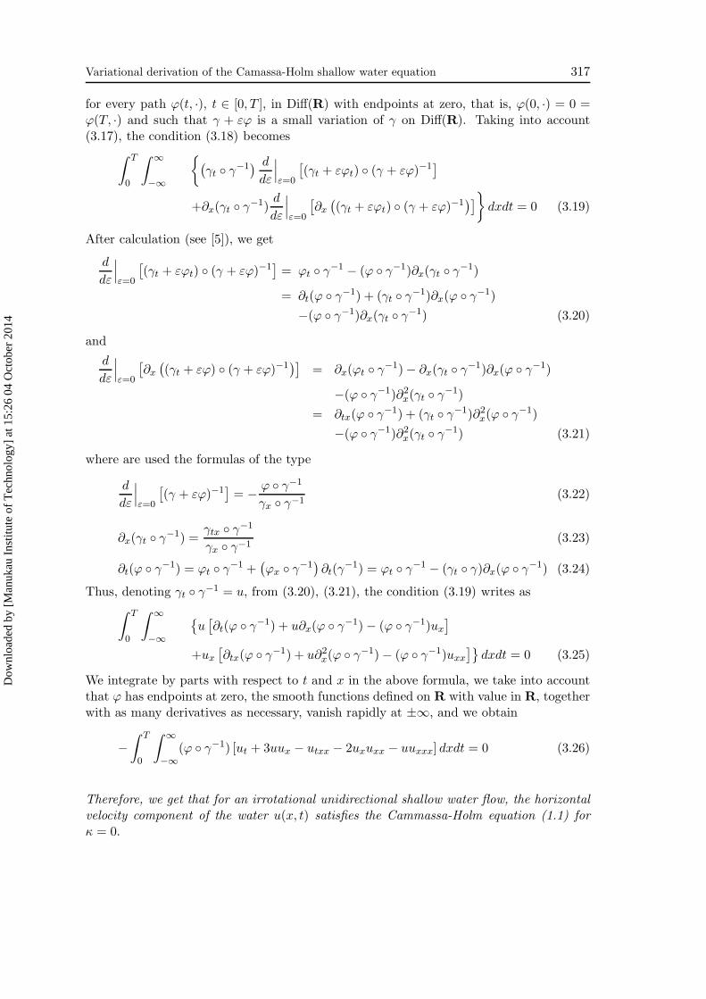
for every path ϕ(t, ·), t ∈ [0, T ], in Diff(R) with endpoints at zero, that is, ϕ(0, ·) = 0 =ϕ(T, ·) and such that γ + εϕ is a small variation of γ on Diff(R). Taking into account(3.17), the condition (3.18) becomes

∫ T

0

∫ ∞

−∞

{

(

γt ◦ γ−1) d

dε

∣

∣

∣

ε=0

[

(γt + εϕt) ◦ (γ + εϕ)−1]

+∂x(γt ◦ γ−1)d

dε

∣

∣

∣

ε=0

[

∂x

(

(γt + εϕt) ◦ (γ + εϕ)−1)]

}

dxdt = 0 (3.19)

After calculation (see [5]), we get

d

dε

∣

∣

∣

ε=0

[

(γt + εϕt) ◦ (γ + εϕ)−1]

= ϕt ◦ γ−1 − (ϕ ◦ γ−1)∂x(γt ◦ γ−1)

= ∂t(ϕ ◦ γ−1) + (γt ◦ γ−1)∂x(ϕ ◦ γ−1)

−(ϕ ◦ γ−1)∂x(γt ◦ γ−1) (3.20)

and

d

dε

∣

∣

∣

ε=0

[

∂x

(

(γt + εϕ) ◦ (γ + εϕ)−1)]

= ∂x(ϕt ◦ γ−1) − ∂x(γt ◦ γ−1)∂x(ϕ ◦ γ−1)

−(ϕ ◦ γ−1)∂2

x(γt ◦ γ−1)

= ∂tx(ϕ ◦ γ−1) + (γt ◦ γ−1)∂2

x(ϕ ◦ γ−1)

−(ϕ ◦ γ−1)∂2

x(γt ◦ γ−1) (3.21)

where are used the formulas of the type

d

dε

∣

∣

∣

ε=0

[

(γ + εϕ)−1]

= − ϕ ◦ γ−1

γx ◦ γ−1(3.22)

∂x(γt ◦ γ−1) =γtx ◦ γ−1

γx ◦ γ−1(3.23)

∂t(ϕ ◦ γ−1) = ϕt ◦ γ−1 +(

ϕx ◦ γ−1)

∂t(γ−1) = ϕt ◦ γ−1 − (γt ◦ γ)∂x(ϕ ◦ γ−1) (3.24)

Thus, denoting γt ◦ γ−1 = u, from (3.20), (3.21), the condition (3.19) writes as

∫ T

0

∫ ∞

−∞

{

u[

∂t(ϕ ◦ γ−1) + u∂x(ϕ ◦ γ−1) − (ϕ ◦ γ−1)ux

]

+ux

[

∂tx(ϕ ◦ γ−1) + u∂2

x(ϕ ◦ γ−1) − (ϕ ◦ γ−1)uxx

]}

dxdt = 0 (3.25)

We integrate by parts with respect to t and x in the above formula, we take into accountthat ϕ has endpoints at zero, the smooth functions defined on R with value in R, togetherwith as many derivatives as necessary, vanish rapidly at ±∞, and we obtain

−∫ T

0

∫ ∞

−∞(ϕ ◦ γ−1) [ut + 3uux − utxx − 2uxuxx − uuxxx] dxdt = 0 (3.26)

Therefore, we get that for an irrotational unidirectional shallow water flow, the horizontalvelocity component of the water u(x, t) satisfies the Cammassa-Holm equation (1.1) forκ = 0.

Dow

nloa

ded

by [

Man

ukau

Ins

titut

e of

Tec

hnol

ogy]

at 1

5:26

04

Oct

ober

201

4

318 Delia Ionescu-Kruse

Let us see now which equation fulfill the displacement η(x, t) of the free surface fromthe flat state. Taking into account (3.15), the kinetic energy on the surface is

K =1

2

∫ ∞

−∞(u2+v2)dx =

1

2

∫ ∞

−∞

[

(η + c0)2 + (1 + ǫη)2η2

x

]

dx ≈ 1

2

∫ ∞

−∞

[

(η + c0)2 + η2

x

]

dx

(3.27)

to the order of our approximation. Transforming K to a right-invariant Lagrangian, theaction on a path Γ(t, ·), t ∈ [0, T ], in Diff(R) is

a(Γ) =1

2

∫ T

0

∫ ∞

−∞{(Γt ◦ Γ−1 + c0)

2 + [∂x(Γt ◦ Γ−1)]2}dxdt (3.28)

The critical points of the action (3.28) in the space of paths with fixed endpoints, verify

d

dεa(Γ + εΦ)

∣

∣

∣

ε=0

= 0, (3.29)

for every path Φ(t, ·), t ∈ [0, T ], in Diff(R) with endpoints at zero, that is, Φ(0, ·) = 0 =Φ(T, ·) and such that Γ + εΦ is a small variation of Γ on Diff(R). Taking into account(3.28), the condition (3.29) becomes

∫ T

0

∫ ∞

−∞

{

(

Γt ◦ Γ−1 + c0) d

dε

∣

∣

∣

ε=0

[

(Γt + εΦt) ◦ (Γ + εΦ)−1]

+∂x(Γt ◦ Γ−1)d

dε

∣

∣

∣

ε=0

[

∂x

(

(Γt + εΦt) ◦ (Γ + εΦ)−1)]

}

dxdt = 0 (3.30)

After calculation, denoting Γt ◦ Γ−1 = η, (3.30) writes as

∫ T

0

∫ ∞

−∞

{

(η + c0)[

∂t(Φ ◦ Γ−1) + η∂x(Φ ◦ Γ−1) − (Φ ◦ Γ−1)ηx

]

+ηx

[

∂tx(Φ ◦ Γ−1) + η∂2

x(Φ ◦ Γ−1) − (Φ ◦ Γ−1)ηxx

]}

dxdt = 0 (3.31)

We integrate by parts with respect to t and x in the above formula, we take into accountthat Φ has endpoints at zero, the smooth functions defined on R with values in R, togetherwith as many derivatives as necessary, vanish rapidly at ±∞, and we obtain

−∫ T

0

∫ ∞

−∞(Φ ◦ Γ−1) [ηt + 3ηηx + 2c0ηx − ηtxx − 2ηxηxx − ηηxxx] dxdt = 0 (3.32)

Therefore, we get that for an irrotational unidirectional shallow water flow, the displace-ment η(x, t) of the free surface from the flat state, satisfies the Camassa-Holm equation(1.1) for κ = c0.

Acknowledgments. I would like to thank Prof. A. Constantin for many interesting anduseful discussions on the subject of water waves and for his kind hospitality at TrinityCollege Dublin.

Dow

nloa

ded

by [

Man

ukau

Ins

titut

e of

Tec

hnol

ogy]

at 1

5:26

04

Oct

ober

201

4

Variational derivation of the Camassa-Holm shallow water equation 319

References

[1] Arnold V., Sur la geometrie differentielle des groupes de Lie de dimension infinie etses applications a l’hydrodynamique des fluids parfaits, Ann. Inst. Fourier (Grenoble)16 (1966), 319–361.

[2] Bressan A., Constantin A., Global conservative solutions of the Camassa-Holmequation, Arch. Rat. Mech. Anal. 183 (2007), 215–239.

[3] Camassa R., Holm D. D., An integrable shallow water equation with peaked soli-tons, Phys. Rev. Letters 71 (1993), 1661–1664.

[4] Constantin A., Existence of permanent and breaking waves for a shallow waterequation: a geometric approach, Ann. Inst. Fourier (Grenoble) 50 (2000), 321–362.

[5] Constantin A., A Lagrangian approximation to the water-wave problem, Appl.Math. Lett. 14 (2001), 789–795.

[6] Constantin A., The trajectories of particles in Stokes waves, Invent. Math. 166

(2006), 523–535.

[7] Constantin A., Escher J., Wave breaking for nonlinear nonlocal shallow waterequations, Acta Mathematica 181 (1998), 229–243.

[8] Constantin A., Gerdjikov V. S., Ivanov R. I., Inverse scattering transform forthe Camassa-Holm equation, Inverse Problems 22 (2006), 2197–2207.

[9] Constantin A., Kolev B., Geodesic flow on the diffeomorphism group of the circle,Comment. Math. Helv. 78(4) (2003), 787–804.

[10] Constantin A., McKean H. P., A shallow water equation on the circle, Comm.Pure Appl. Math. 52 (1999), 949–982.

[11] Constantin A., Strauss W., Exact steady periodic water waves with vorticity,Comm. Pure Appl. Math. 57 (2004), 481–527.

[12] Fokas A. S., Fuchssteiner B., Symplectic structures, their Backlund transforma-tions and hereditary symmetries, Physica D 4 (1981), 47–66.

[13] Fuchssteiner B., The Lie algebra structure of nonlinear evolution equations ad-mitting infinite dimensional abelian symmetry groups, Prog. Theor. Phys. 65 (1981),861–876.

[14] Fuchssteiner B., Some tricks from the symmetry-toolbox for nonlinear equations:Generalizations of the Camassa-Holm equation, Physica D 95 (1996), 229–243.

[15] Johnson R. S., A Modern Introduction to the Mathematical Theory of Water Waves,Cambridge Univeristy Press, 1997.

[16] Johnson R. S., Camassa-Holm, Korteweg-de Vries and related models for waterwaves, J. Fluid Mech. 455 (2002), 63–82.

Dow

nloa

ded

by [

Man

ukau

Ins

titut

e of

Tec

hnol

ogy]

at 1

5:26

04

Oct

ober

201

4

320 Delia Ionescu-Kruse

[17] Johnson R. S., The Camassa-Holm equation for water waves moving over a shearflow, Fluid Dynamics Research, 33 (2003), 97–111.

[18] Kunze S., Schneider G., Estimates for the KdV-limit of the Camassa-Holm equa-tion, Lett. Math. Phys. 72 (2005), 17–26.

[19] Misiolek, G., A shallow water equation as a geodesic flow on the Bott-Virasorogroup, J. Geom. Phys. 24 (1998), 203–208.

Dow

nloa

ded

by [

Man

ukau

Ins

titut

e of

Tec

hnol

ogy]

at 1

5:26

04

Oct

ober

201

4