value-at-risk: a multivariate switching regime approachsmartquant.com/references/var/var2.pdf ·...

Ž .Journal of Empirical Finance 7 2000 531–554www.elsevier.comrlocatereconbase

Value-at-Risk: a multivariate switching regimeapproach

Monica Billio a,), Loriana Pelizzon b,c

a Dipartimento di Scienze Economiche, UniÕersita Ca’ Foscari, Fondamenta San Giobbe 873,`30121 Venice, Italy

b London Business School, London, UKc UniÕersity of Padua, Padua, Italy

Accepted 5 October 2000

Abstract

This paper analyses the application of a switching volatility model to forecast theŽ .distribution of returns and to estimate the Value-at-Risk VaR of both single assets and

portfolios. We calculate the VaR value for 10 Italian stocks and a number of portfoliosbased on these stocks. The calculated VaR values are also compared with the variance–co-

Ž .variance approach used by JP Morgan in RiskMetricse and GARCH 1,1 models. Underbacktesting, the VaR values calculated using the switching regime beta model are preferred

wto both other methods. The Proportion of Failure and Time Until First Failure tests TheŽ . xJournal of Derivatives 1995 73–84 confirm this result. q 2000 Elsevier Science B.V. All

rights reserved.

JEL classification: C22; C52; G28Keywords: Value-at-Risk; Switching regime models; Multivariate approach; Factors models

1. Introduction

Ž .Value at Risk VaR is a risk-management technique that has been widely usedto assess market risk. VaR for a portfolio is simply an estimate of a specifiedpercentile of the probability distribution of the portfolio’s value change over a

) Corresponding author. Tel.: q39-041-257-4170; fax: q39-041-257-4176.Ž .E-mail address: [email protected] M. Billio .

0927-5398r00r$ - see front matter q2000 Elsevier Science B.V. All rights reserved.Ž .PII: S0927-5398 00 00022-0

( )M. Billio, L. PelizzonrJournal of Empirical Finance 7 2000 531–554532

given holding period. The specified percentile is usually in the lower tail of thedistribution, e.g., the 95th percentile or the 99th percentile.

Calculation of portfolio VaR is often based on the variance–covariance ap-proach and makes the assumption, among others, that returns follow a conditionalnormal distribution. We show that this assumption is at odds with reality and oftenresults in misleading estimates of VaR.

Ž .There is substantial empirical evidence Hsieh, 1988; Meese, 1986 that thedistribution of returns on equities and other assets is typically leptokurtic, that is,the unconditional return distribution shows high peaks and fat tails. This featurecan arise from a number of different reasons, in particular: jumps, correlationbetween shocks and changes in volatility, and time series volatility fluctuationsusually characterized by persistence.

The literature commonly describes persistence in time series volatility usingARCH or GARCH models that give rise to unconditional symmetric and leptokur-tic distributions. Here leptokurtosis follows from persistence in the conditionalvariance, which produces the clusters of Alow volatilityB and Ahigh volatilityBreturns.

In RiskMetricse, volatility is estimated using the exponentially weightedŽ .moving average EWMA approach, which places more emphasis on more recent

Ž .history in estimating volatility. As Phelan 1995 demonstrates, this approach is arestrictive case of the GARCH model.

However, these models do not account for jumps in stock returns. Nevertheless,as risk measurement focuses in particular on the AtailsB distribution, jumps deservecareful study.

For this reason, we suggest a new and relatively simple method for estimatingŽ .VaR: the Aswitching regime approachB. This approach is able to i consider the

Ž .conditional non-normality of returns, ii take into account time-varying volatilityŽ .characterized by persistence, and iii deal with events that are relatively infre-

Ž .quent e.g., some changes in the level of volatility .The solutions proposed in the VaR literature to the last problem have been the

Ž . Ž . Ž .use of: i the ex-post historical simulation approach, ii the ex-ante Student’sŽ .t-distributions, and iii a mixture of two normal distribution, as proposed by

Ž .RiskMetrics Longerstay, 1996 .Each of these solutions is only partially able to deal with the problems of

skewness and kurtosis in the return distribution as they do not entirely correct theunder-estimation of risk.

In the financial literature, the non-normality of asset returns has attractedparticular attention both as a problem in its own, and because of its implicationsfor the evaluation of contingent claims, in particular options. A number ofdifferent time series models have been employed to capture these distributional

Žfeature: stationary fat-tailed distributions such as Student’s t Rogalski and Vinso,. Ž .1978 and the jump diffusion process Akgiray and Booth, 1988 ; Gaussian ARCH

Ž .or GARCH models Bollerslev et al., 1992 ; chaotic models; non-standard classes

( )M. Billio, L. PelizzonrJournal of Empirical Finance 7 2000 531–554 533

Ž .of stochastic processes such as stable processes see Mandelbrot, 1963 , andŽsubordinated stochastic processes Clark, 1973; Geman and Ane, 1996; Muller et´ ¨

.al., 1993 .In our paper we model this phenomenon using the Aswitching regimeB ap-

proach that gives rise to a non-normal return distribution in a simple and intuitiveway. The improved forecast of return distribution obtained with this approach isimportant since VaR methodology is indeed based on forecasting the distributionof future values of a portfolio.

ŽThe approach is similar to the mixture of distributions proposed by JP Morgan.to embed skewness and kurtosis in a VaR measure , but with the difference that

the unobserved random variable characterizing the regime is the outcome of anunobserved k-state Markov chain instead of a Bernoulli variable. The advantage ofusing a Markov chain as opposed to a Bernoulli specification is that the formerallows conditional information to be reflected in the forecast and it captures thewell known fact that high volatility is usually followed by high volatility.

The purpose of this paper is to describe the application of this approach to theestimation of VaR and so allow for a more realistic model of the tail distributionof financial returns. We focus on the measurement of market risk in equityportfolios and illustrate our method using data on 10 Italian stocks and the MIB30Italian Index.

The plan of the paper is as follows. Section 2 provides a description of theevaluation framework for VaR estimates. Section 3 describes the different switch-ing regime models used to estimate VaR. Section 4 shows the results of theempirical investigation of these models on the Italian equity market and compares

Ž . Ž . Ž .the results with i RiskMetrics and ii GARCH 1,1 approaches. Section 5concludes.

2. Evaluation of VaR estimates

2.1. VaR definition

VAR is a measure of market risk for a portfolio of financial assets1 andmeasures the level of loss that a portfolio could lose, with a given degree ofconfidence a, over a given time horizon h. Analytically it can be formulated asfollows:

Pr W yW -yVaR h sa 1Ž . Ž .tqh t W

Ž .where W is the portfolio value at time t and VaR h is the VaR value of thet W

portfolio W with a time horizon h.

1 There is an extensive recent literature on VaR. Nevertheless, for an introduction to VaR seeŽ .Linsmeier and Pearson 1996 .


Ž .The confidence level 1ya is typically chosen to be at least 95% and often asŽ .high as 99% or more a equal to 5% or 1% . The time horizon h varies with the

use made of VaR by management and asset liquidity.It is possible to express the VaR measure in terms of return of the portfolio

instead of portfolio value. Analytically it can be formulated as follows:

Pr R -yVaR h sa 2Ž . Ž .W Rtq h

Ž . Ž .where R s ln W rW is the portfolio return at time tqh and VaR h isW tqh t Rtq h

the VaR value of portfolio returns R with a time horizon h.W

Clearly, VaR is simply a specific quantile of a portfolio’s potential lossdistribution over a given holding period.

Assuming R ; f , where f is a general return distribution, the VaR for timeW t tt

tqh, estimated using a model indexed by m, conditional on the informationŽ .available at time t and denoted VaR h,a , is the point in f model m’sm mtqh

estimated return distribution that corresponds to its lower a percent tail. That isŽ .VaR h,a is the solution to:m

Ž .VaR h ,am f x d xsa 3Ž . Ž .H mtqhy`

Different models can be used to forecast the return distribution and so tocalculate VaR. Given the widespread use of VaR by banks and regulators, it isimportant to determine the accuracy of the different models used to estimate VaR.

2.2. AlternatiÕe eÕaluation methods

Ž .As discussed by Kupiec 1995 a variety of methods are available to test thenull hypothesis that the observed probability of occurrence over a reporting periodequals a. In our work, two methods are used to evaluate the accuracy of the VaR

Ž . Ž .model: the Proportion of Failure PF test Kupiec, 1995 and the time until firstŽ . Ž .failure TUFF test Kupiec, 1995 .

The first test is based on the probability under the binomial distribution ofobserving x exceptions in the sample size T.2 In particular:

TyxT xPr x ;a,T s a 1ya 4Ž . Ž . Ž .ž /xVaR estimates must exhibit that their unconditional coverage a, measured by

Ž .asxrT , equals the desired coverage level a usually equal to 1% or 5% . Thus,ˆ 0

2 Ž .x exceptions means the number of times the observed value R is lower than VaR h .W Rtqh


the null hypothesis is H : asa , and the corresponding Likelihood ratio statistic0 0

is:

Tyx Tyxx xLR s2 ln a 1ya y ln a 1ya 5Ž . Ž . Ž .ˆ ˆŽ . Ž .PF 0 0

2Ž .which is asymptotically distributed as x 1 .The TUFF test is based on the number of observations before the first

exception. The relevant null hypothesis is, once again, H : asa and the0 0

Likelihood ratio statistic is:

T̃y1T̃y1˜ ˜ ˜LR T ,a sy2ln a 1ya q2ln 1rT 1y1rT 6Ž . Ž .Ž .ˆ ˆ ˆ Ž . Ž .TUFF

˜where T denotes the number of observations before the first exception. The2Ž .LR test statistic is also asymptotically distributed as x 1 .TUFF

Unfortunately, as Kupiec observed, these tests have a limited power to distin-guish among alternative hypotheses. However, this approach has been adopted by

Žregulators in the analysis of internal models to define the zones green, yellow and.red into which the different models are categorized in backtesting. In particular,

for a backtest with 250 observations, regulators place a model in the green zone ifŽ .x the exception number is lower than 4; from 5 to 9 these models are allocated to

the yellow zone and the required capital is increased by an incremental factor thatranges from 0.4 to 0.85. If x is greater than 9, the incremental factor is 1.

3. Switching regime models

The risk profile of a firm or of the economy as a whole does not remainconstant over time. A variety of systematic and unsystematic events may changethe business and financial risk of firms significantly. It is argued here that thismight derive from the presence of discontinuous shifts in return volatility.

The change in regime should not be regarded as predictable but as a randomevent. The effect of these risk shifts should be taken into account by risk analystsin the forecasting process, by risk managers in the assessment of market risk andcapital allocation, and by regulators, in the definition of capital requirements.

3.1. Simple switching regime models

Ž .A Simple Switching Regime Model SSRM can be written as:

R sm s qs s ´ 7Ž . Ž . Ž .t t t t


Ž . Ž .where R s ln P rP , ´ ; IIN 0,1 , P is the stock price or the index price, st t ty1 t t t

is a Markov chain with k states and transition probability matrix P. In particularif ks2, we have:

m qs ´ if s s00 0 t tR st ½m qs ´ if s s11 1 t t

and the transition matrix P is:

p 1ypPs 8Ž .

1yq q

where the parameters p and q are probabilities that volatility remains in the sameregime. In the model, the variance and mean of returns change only as a result ofperiodic, discrete events.3

Ž .Switching regime models have been applied by Rockinger 1994 and vanŽ .Norden and Schaller 1993 to stock market returns, assuming that returns are

characterized by a mixture of distributions. This gives rise to a fat-tailed distribu-tion, a feature of the return data which has been extensively documented since the

Ž .early work by Mandelbrot 1963 .This approach is different to the mixture of two normal distributions proposed

Ž .by JP Morgan as a new methodology for measuring VaR Longerstay, 1996 . Inthe JP Morgan approach, the discontinuous shift random variable is a Bernoullivariable, that is, s assumes the values 0 and 1 with respective probabilities of pt

Ž . Ž .and 1yp . The future value of this variable s is independent of the valuetq1

s , that is, future values of the state variable are independent on the current state.t

In the JP Morgan approach the distribution of future returns depends only on theunconditional probabilities of the Markov chain:

1yq r 2ypyqŽ . Ž .ps 9Ž .

1yp r 2ypyqŽ . Ž .

instead of the conditional probabilities p and q. The two approaches are the sameonly if p and q are equal to 0.5.

3 Switching regime models is a methodology that has encountered great success in macroeconomicsŽ . Žapplications. In the path-breaking works by Quandt 1958 , as well as Goldfeld and Quandt 1973,

. Ž .1975 it was used to describe markets in disequilibrium. Hamilton 1989, 1994 has brought about aŽ .Renaissance of this methodology by modelling business cycles. In Engel and Hamilton 1990 , the

switching approach is successfully applied to exchange rates. Firstly, applications to finance have beenŽ . Ž .scarce, noteworthy exceptions being Pagan and Schwert 1990 , Turner et al. 1989 , as well as van

Ž . Ž . Ž .Norden and Schaller 1993 , Rockinger 1994 and Hamilton and Susmel 1994 . Now there is highŽ . Ž .interest for this type of models: see for example, Billio and Pelizzon 1997 , Ang and Bekaert 1999 ,

Ž . Ž . Ž .Campbell and Li 1999 , Khabie-Zeitoun et al. 1999 , Jeanne and Masson 1999 .


The advantage of using a Markov chain as opposed to a Bernoulli specificationfor the random discontinuous shift is that the former allows to conditional

Ž .information to be used in the forecasting process. This allows us to: i fit andŽ .explain the time series, ii capture the well known cluster effect, under which

Žhigh volatility is usually followed by high volatility in presence of persistent. Ž .regimes , iii generate better forecasts compared to the mixture of distributions

model, since switching regime models generate a time conditional forecast distri-bution rather than an unconditional forecasted distribution.

To calculate the VaR, under the SSRM process, it is necessary to determine thecritical value of the conditional distribution for which the cumulative density is a.

Ž .Assuming ks2, the critical value and so the VaR is defined as:

VaR 2< <as Pr s I N x ,m s ,s s I d x 10Ž . Ž . Ž .Ž . Ž .Ý Htqh t tqh tqh ty`s s0,1tqh

where N is the normal distribution, I is the available information at date t,tŽ < . Ž . Ž .Pr s I is obtained by the Hamilton’s filter see Hamilton, 1994 , m s andtqh t tqh

2Ž . Ž . Ž .s s are respectively the mean and the variance with m 0 sm , m 1 sm ,tqh 0 12Ž . 2 2Ž . 2s 0 ss and s 1 ss .0 1

The SSRM we present above is a special case of other, more general, switchingregime models that we present below.

3.2. Switching regime beta models

The SSRM does not provide an explicit link between the return on the stockŽ .and the return on the market index. The Switching Regime Beta Model SRBM is

a sort of market model or better a single factor model in the APT frameworkwhere the return of a single stock i is characterized by the regime switching of themarket index and the regime switching of the specific risk of the asset. The SRBMcan be written as:

R sm s qs s ´ , ´ ; IIN 0,1Ž . Ž . Ž .mt m t m t t t11Ž .½R sm s qb s ,s R qs s ´ , ´ ; IIN 0,1Ž . Ž . Ž . Ž .i t i i t i t i t m t i i t i t i t

where s and s are two independent Markov chains and ´ and ´ aret i t i t t

independently distributed.In such a framework the conditional mean of the risky asset is given by the

Ž . Ž Ž ..parameter m s that is specific to the asset plus the factor loading b s , si i t i t i, t

on the conditional mean of the factor. The factor loading compensates for the riskof the asset, which depends on the factor: higher covariances demand higher riskpremium. The variance is the sum of variance of the index market weighted by thefactor loading and the variance of the idiosyncratic risk.


To calculate VaR, we use the approach as before. Assuming that ks2 for boththe Markov chains we have:

Var<as Pr s ,s I N x ,m s ,s ,Ž .Ž . ŽÝ Ý Htqh i , tqh t tqh i , tqh

y`s s0,1s s0,1tqh i , tqh

2 <s s ,s I d x 12Ž . Ž ..tqh i , tqh t

Ž . Ž . Žwhere N is the normal distribution with m s , s sm s qb s ,tqh i, tqh i i, tqh i tqh. Ž . 2Ž . 2Ž . 2Ž . 2Ž .s m s and s s , s sb s , s s s qs s ,i, tqh m tqh tqh i, tqh i tqh i, tqh m tqh i i, tqh

Ž < .I is the available information at date t and Pr s , s I is obtained, ast tqh i, tqh t

before, by the Hamilton filter.The SRBM considers a single asset only, but can be generalized to calculate the

VaR for a portfolio of assets taking into account the correlation between differentassets.

3.3. MultiÕariate switching regime model

The generalized version of the SRBM, considering N risky assets, that we callŽ .the Multivariate Switching Regime Model MSRM , can be written as:

°R sm s qs s ´ , ´ ; IIN 0,1Ž . Ž . Ž .mt m t m t t t

R sm s qb s ,s R qs s ´ , ´ ; IIN 0,1Ž . Ž . Ž . Ž .1 t 1 1 t 1 t 1 t m t 1 1 t 1 t 1 t

~R sm s qb s ,s R qs s ´ , ´ ; IIN 0,1Ž . Ž . Ž . Ž . 13Ž .2 t 2 2 t 2 t 2 t m t 2 2 t 2 t 2 t...¢R sm s qb s ,s R qs s ´ , ´ ; IIN 0,1Ž . Ž . Ž . Ž .N t N N t N t N t mt N N t N t N t

where s and s , js1, . . . , N are independent Markov chains, ´ and ´ ,t jt t jt

js1, . . . , N, are independently distributed.Using this approach we are able to take into account the correlation between

different assets. In fact, if we consider ks2, two assets, and, for example,s ss s0 and s s1, the variance–covariance matrix between the two assets is:t 1 t 2 t

2 2 2 2b 0,0 s 0 qs 0 b 0,0 b 0,1 s 0Ž . Ž . Ž . Ž . Ž . Ž .1 m 1 1 2 mS 0,0,1 s 14Ž . Ž .

2 2 2 2b 0,1 b 0,0 s 0 b 0,1 s 0 qs 1Ž . Ž . Ž . Ž . Ž . Ž .2 1 m 2 m 2

then the correlation between different assets is given by b ’s parameters andmarket variance.

In this model, as in the market model, the covariance between asset 1 and asset2 depends on the extent to which each asset is linked, through the factor loadingb , to the market index.


To calculate VaR for a portfolio based on N assets it is enough to use theapproach presented above. In particular, considering two assets and assuming thatks2 for all the three Markov chains we have:

<as Pr s ,s ,s IŽ .Ý Ý Ý tqh 1, tqh 2, tqh ts s0,1s s0,1s s0,1tqh 1, tqh 2, tqh

=VaR XN x ,wm s ,s ,s ,Ž .ŽH tqh 1, tqh 2, tqh

y`

X <wS s ,s ,s w I d x 15Ž . Ž ..tqh 1, tqh 2, tqh t

where w is the vector of the percentage of wealth invested in the two assets andŽ .m s , s , s is the vector of risky asset mean returns based on the singletqh 1, tqh 2, tqh

asset mean returns already described in the SRBM. For example with s ss s0t 1 t

and s s1, we have:2 t

m 0 qb 0,0 m 0Ž . Ž . Ž .1 1 mm 0,0,1 s 16Ž . Ž .½m 1 qb 0,1 m 0Ž . Ž . Ž .2 2 m

However, MSRM requires the estimation of a number of parameters that growsexponentially with the number of assets. In fact, the number of possible regimesgenerates by this model is 2 Nq1.

3.4. The factor switching regime model

One possible solution to the problem that affects the MSRM is to consider theŽ 2 . Žspecific risk distributed as IIN 0,s without a specific Markov chain depen-i

.dency and characterize the systematic risk with more than one source of risk. ThisŽ Ž ..approach that we call Factor Switching Regime Model FSRM is in line with

the Arbitrage Pricing Theory Model where the risky factors are characterized byswitching regime processes. Formally, we can write this model as:

°F sa s qu s ´ , ´ ; IIN 0,1Ž . Ž . Ž .jt j jt j jt jt jt

g

R sm q b s F qs ´ , ´ ; IIN 0,1Ž . Ž .Ý1 t 1 1 j jt jt 1 1 t 1 tjs1

g

~R sm q b s F qs ´ , ´ ; IIN 0,1Ž . Ž .Ý 17Ž .2 t 2 2 j jt jt 2 2 t 2 tjs1

...g

R sm q b s F qs ´ , ´ ; IIN 0,1Ž . Ž .ÝN t N N j jt jt N N t N t¢js1


Ž . Ž .where F is the value of factor j at time t js1,2, . . . , g , b s is the factorjt i jt

loading of asset i on factor j and s is the Markov chain that characterizes factorjt

j. Further, s , js1, . . . , g are independent Markov chains, ´ , js1, . . . , g, andjt jt

´ , is1, . . . , N, are independently distributed.i t

The FSRM is more parsimonious, in fact the introduction of an extra assetmeans that only gq2 parameters need to be estimated.

This approach is valid when the number of assets in the portfolio is high andthe specific risk is easily eliminated by diversification.

Using this approach, the variance–covariance matrix is simply:

2 2 2 2 2Ž . Ž . Ž . Ž . Ž . Ž . Ž . Ž .b s u s qs b s b s u s PPP b s b s u s1 t t 1 1 t 2 t t 1 t N t t

2 2 2 2Ž . Ž . Ž . Ž . Ž .b s b s u s b s u s qs PPP PPP2 t 1 t t 2 t t 2Ž .S s stPPP PPP PPP PPP

2 2 2 2Ž . Ž . Ž . Ž . Ž .b s b s u s PPP PPP b s u s qsN t 1 t t N t t N

18Ž .

The VaR for a portfolio based on N assets, one factor and ks2 is defined as:

VaR X X< <as Pr s I N x ,wm s ,w S s w I d x 19Ž . Ž . Ž .Ž . Ž .Ý Htqh t tqh tqh ty`s s0,1tqh

Ž .where m s is the vector of risky assets mean returns, that is:tqh

m qb s a sŽ . Ž .1 1 tqh tqh

m qb s a sŽ . Ž .2 2 tqh tqhm s s 20Ž . Ž .tqhPPP

m qb s a sŽ . Ž .N N tqh tqh

4. VaR estimation

4.1. VaR estimation of a single asset

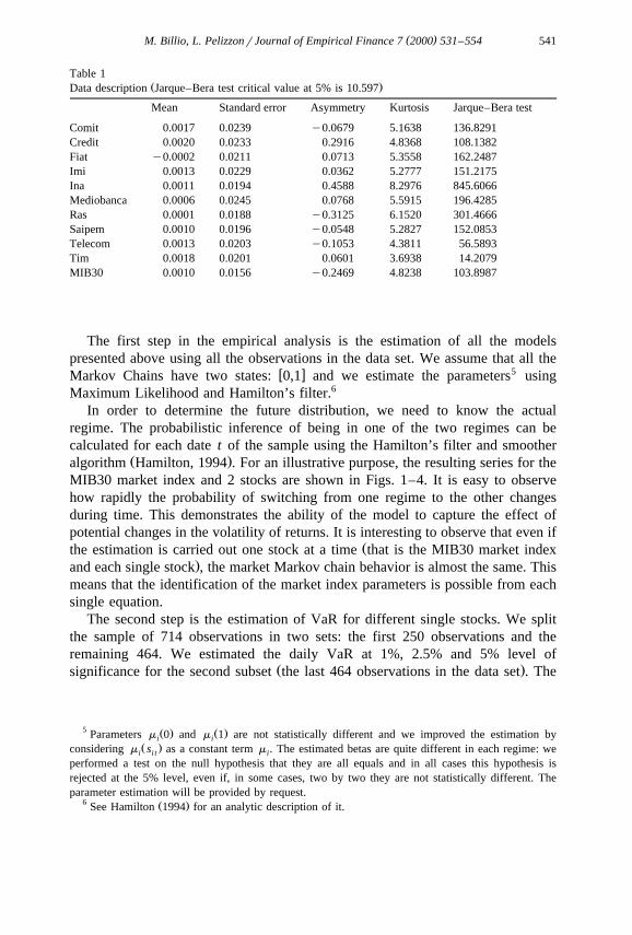
The data used in the empirical analysis are daily returns based on closing priceof 10 Italian Stocks4 and the MIB30 Italian market index. The data cover theperiod from November 29, 1995 to September 30, 1998: a total of 714 dailyobservations. Table 1 gives summary statistics and a normality test: all the seriesfail to pass the Jarque–Bera normality test.

4 Comit, Credit, Fiat, Imi, Ina, Mediobanca, Ras, Saipem, Telecom, Tim.


Table 1Ž .Data description Jarque–Bera test critical value at 5% is 10.597

Mean Standard error Asymmetry Kurtosis Jarque–Bera test

Comit 0.0017 0.0239 y0.0679 5.1638 136.8291Credit 0.0020 0.0233 0.2916 4.8368 108.1382Fiat y0.0002 0.0211 0.0713 5.3558 162.2487Imi 0.0013 0.0229 0.0362 5.2777 151.2175Ina 0.0011 0.0194 0.4588 8.2976 845.6066Mediobanca 0.0006 0.0245 0.0768 5.5915 196.4285Ras 0.0001 0.0188 y0.3125 6.1520 301.4666Saipem 0.0010 0.0196 y0.0548 5.2827 152.0853Telecom 0.0013 0.0203 y0.1053 4.3811 56.5893Tim 0.0018 0.0201 0.0601 3.6938 14.2079MIB30 0.0010 0.0156 y0.2469 4.8238 103.8987

The first step in the empirical analysis is the estimation of all the modelspresented above using all the observations in the data set. We assume that all the

w x 5Markov Chains have two states: 0,1 and we estimate the parameters usingMaximum Likelihood and Hamilton’s filter.6

In order to determine the future distribution, we need to know the actualregime. The probabilistic inference of being in one of the two regimes can becalculated for each date t of the sample using the Hamilton’s filter and smoother

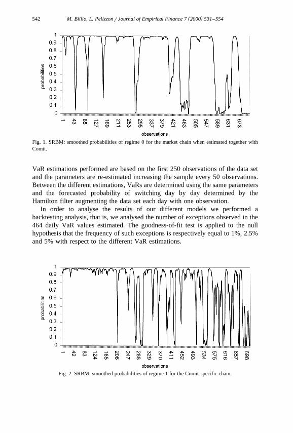
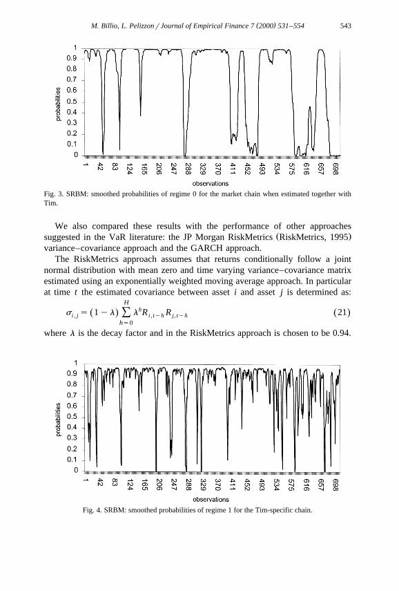
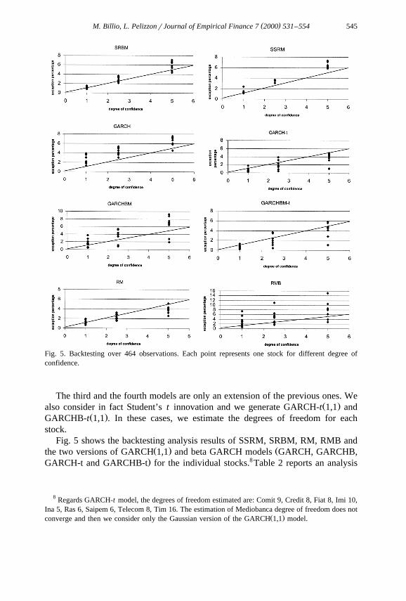
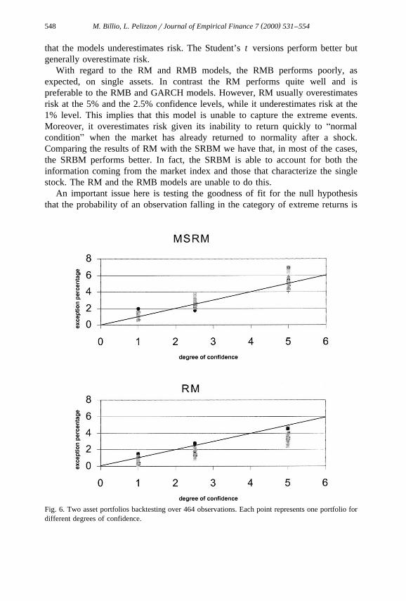
Ž .algorithm Hamilton, 1994 . For an illustrative purpose, the resulting series for theMIB30 market index and 2 stocks are shown in Figs. 1–4. It is easy to observehow rapidly the probability of switching from one regime to the other changesduring time. This demonstrates the ability of the model to capture the effect ofpotential changes in the volatility of returns. It is interesting to observe that even if

Žthe estimation is carried out one stock at a time that is the MIB30 market index.and each single stock , the market Markov chain behavior is almost the same. This

means that the identification of the market index parameters is possible from eachsingle equation.

The second step is the estimation of VaR for different single stocks. We splitthe sample of 714 observations in two sets: the first 250 observations and theremaining 464. We estimated the daily VaR at 1%, 2.5% and 5% level of

Ž .significance for the second subset the last 464 observations in the data set . The

5 Ž . Ž .Parameters m 0 and m 1 are not statistically different and we improved the estimation byi iŽ .considering m s as a constant term m . The estimated betas are quite different in each regime: wei i t i

performed a test on the null hypothesis that they are all equals and in all cases this hypothesis isrejected at the 5% level, even if, in some cases, two by two they are not statistically different. Theparameter estimation will be provided by request.

6 Ž .See Hamilton 1994 for an analytic description of it.


Fig. 1. SRBM: smoothed probabilities of regime 0 for the market chain when estimated together withComit.

VaR estimations performed are based on the first 250 observations of the data setand the parameters are re-estimated increasing the sample every 50 observations.Between the different estimations, VaRs are determined using the same parametersand the forecasted probability of switching day by day determined by theHamilton filter augmenting the data set each day with one observation.

In order to analyse the results of our different models we performed abacktesting analysis, that is, we analysed the number of exceptions observed in the464 daily VaR values estimated. The goodness-of-fit test is applied to the nullhypothesis that the frequency of such exceptions is respectively equal to 1%, 2.5%and 5% with respect to the different VaR estimations.

Fig. 2. SRBM: smoothed probabilities of regime 1 for the Comit-specific chain.


Fig. 3. SRBM: smoothed probabilities of regime 0 for the market chain when estimated together withTim.

We also compared these results with the performance of other approachesŽ .suggested in the VaR literature: the JP Morgan RiskMetrics RiskMetrics, 1995

variance–covariance approach and the GARCH approach.The RiskMetrics approach assumes that returns conditionally follow a joint

normal distribution with mean zero and time varying variance–covariance matrixestimated using an exponentially weighted moving average approach. In particularat time t the estimated covariance between asset i and asset j is determined as:

Hhs s 1yl l R R 21Ž . Ž .Ýi , j i , tyh j , tyh

hs0

where l is the decay factor and in the RiskMetrics approach is chosen to be 0.94.

Fig. 4. SRBM: smoothed probabilities of regime 1 for the Tim-specific chain.


For the RiskMetrics variance–covariance model we considered both the ap-proach suggested by JP Morgan where the VaR for each asset is based on its

Ž .volatility we call this RM and the approach for equities: where the calculation isŽbased on the risk of the Market index and the beta of the stocks we call this

.RMB . Specifically, in the RM model we have:

VaR sF a s 22Ž . Ž .(i i , i

Ž .where: VaR is the VaR of the generic stock i, F a is the cumulate standardi

normal distribution coefficient, s is the asset i variance.i, i

In the RMB model we calculate VaR as:

VaR sb VaR 23Ž .i i ,m m

where: VaR is the VaR of the Market index, b s is the beta of the beta ofm i,m

asset i with respect to the market index.For VaR calculation based on RiskMetrics approach we used a moving window

of 250 observations.Regards the GARCH approach we consider four models. The first is a GARCH

Žmodel with conditional normal distribution and zero mean in line with the.RiskMetrics approach . In particular, we assume that returns follows a

Ž .GARCH 1,1 , that is:

R su sh ´ 24Ž .t t t t

Ž . Ž 2 < . 2 2 2where: ´ ;N 0,1 , E u I 'h saqbu qgh , I is the informationt t ty1 t ty1 ty1 t

set.With this model we have:

VaR sF a h 25Ž . Ž .i tq1

where: h is the GARCH asset i variance.tq1Ž .The second is a beta-GARCH model or one factor model , that we call

GARCHB, with the following return specification:

R sm qu ,mt m mt26Ž .½R sa qb R qu ,i t i i m t i t

Ž . Ž 2 . 2 2 2where: u sh ´ , ´ ;N 0,1 , E u N I 'h saqbu qgh , uit i t i t i t i t ty1 i t i, ty1 i, ty1 m , tŽ . Ž 2 . 2 2 2s s ´ , ´ ; N 0,1 , E u N I ' s s a q b u q g s ,m , t m t mt mt ty1 m , t m m m , ty1 m m , ty1

Ž < .Cov u , R I s0.i t m , t ty1

With this model we have7:

VaR sm qF a s 27Ž . Ž .i i , tq1 i , tq1

Ž < .w here: m s a q b E R I s a q b m , s i , t q 1i , tq 1 i i m , tq 1 t i i m , t2 2 2(s b s qh .I m , tq1 i , tq1

7 Ž .For a derivation of conditional moments in a factor model see Gourieroux 1992, p. 218 .´


Fig. 5. Backtesting over 464 observations. Each point represents one stock for different degree ofconfidence.

The third and the fourth models are only an extension of the previous ones. WeŽ .also consider in fact Student’s t innovation and we generate GARCH-t 1,1 and

Ž .GARCHB-t 1,1 . In these cases, we estimate the degrees of freedom for eachstock.

Fig. 5 shows the backtesting analysis results of SSRM, SRBM, RM, RMB andŽ . Žthe two versions of GARCH 1,1 and beta GARCH models GARCH, GARCHB,

. 8GARCH-t and GARCHB-t for the individual stocks. Table 2 reports an analysis

8 Regards GARCH-t model, the degrees of freedom estimated are: Comit 9, Credit 8, Fiat 8, Imi 10,Ina 5, Ras 6, Saipem 6, Telecom 8, Tim 16. The estimation of Mediobanca degree of freedom does not

Ž .converge and then we consider only the Gaussian version of the GARCH 1,1 model.


Table 2Mean absolute error of a-values over 10 single asset portfolios

) Ž .a % SRBM SSRM GARCH GARCH-t GARCHB GARCHB-t RM RMB

5 0.009 0.014 0.017 0.012 0.025 0.013 0.011 0.0352.5 0.004 0.009 0.019 0.010 0.017 0.009 0.005 0.0261 0.002 0.004 0.014 0.004 0.011 0.004 0.005 0.020

of the mean absolute difference between the observed and theoretical confidencelevel.

Table 3Ž . Žp-Values of the Proportion of Failure test PF for the different models given the poor performance of

.SSRM and RMB models we avoid to present their test value

PF test Degree of SRBM GARCH GARCHB GARCH-t GARCHB-t RMconfidence p-value p-value p-value p-value p-value p-valueŽ . Ž . Ž . Ž . Ž . Ž . Ž .% % % % % % %

Comit 5.0 42.96 96.60 16.50 35.63 55.81 24.972.5 7.02 7.79 2.33 48.92 13.28 68.291.0 1.32 0.04 0.00 86.82 54.38 7.16

Credit 5.0 42.96 3.09 4.90 3.50 1.82 0.882.5 62.62 1.19 21.55 0.91 2.71 25.721.0 86.82 15.52 30.57 41.33 16.48 41.33

Fiat 5.0 13.28 4.90 7.55 79.66 63.41 35.632.5 86.82 13.28 2.33 14.02 85.71 14.021.0 66.86 54.38 15.52 75.97 41.33 75.97

Imi 5.0 3.09 3.09 0.06 16.64 79.66 48.552.5 85.72 21.56 2.33 25.72 42.12 85.721.0 30.58 0.35 54.38 86.82 75.97 7.16

Ina 5.0 16.50 3.09 1.90 35.63 35.63 86.542.5 21.56 0.05 0.05 14.02 14.02 48.921.0 54.38 0.00 0.00 3.95 16.49 0.35

Mediobanca 5.0 16.50 4.36 0.06 16.642.5 21.56 3.02 2.71 62.621.0 86.82 0.33 41.33 75.97

Ras 5.0 37.45 0.27 1.82 0.00 0.00 24.972.5 27.35 0.04 0.91 0.04 0.00 62.621.0 41.82 0.02 16.49 16.49 16.49 54.38

Saipem 5.0 23.36 4.36 0.06 16.64 35.63 33.312.5 13.28 7.16 0.12 25.72 85.72 7.161.0 31.64 0.35 0.14 41.33 75.98 1.32

Telecom 5.0 64.96 4.36 64.96 36.60 79.66 48.552.5 16.50 3.02 16.50 25.72 42.12 85.721.0 31.64 0.35 31.64 41.33 41.33 54.38

Tim 5.0 70.48 11.32 11.32 48.55 42.96 6.252.5 68.29 3.02 7.79 85.72 21.56 86.821.0 30.58 1.32 3.02 41.33 75.97 82.92


From Fig. 5 and Table 2 it is evident that the SRBM performs quite well foralmost every percentile and every stock. In fact the results are close to thetheoretical values and it does not seem that the model persistently either under orover estimates any of the confidence level. In particular, it is interesting to observethat the SRBM performs always better than the SSRM, which suggests that thelink with the market is fundamental to risk estimation.

Moreover, the SRBM performs better than all GARCH models. In fact theGaussian GARCH and GARCHB models do not work very well as the number ofextreme observations deviates significantly from the theoretical values for almostall the stocks. Generally, the values are higher than the theoretical ones and means

Table 4Ž .p-Values of the Time Until First Failure Test TUFF for the different models

TUFF test Degree of SRBM GARCH GARCHB GARCH-t GARCHB-t RMconfidence p-value p-value p-value p-value p-value p-valueŽ . Ž . Ž . Ž . Ž . Ž . Ž .% % % % % % %

Comit 5.0 1.44 1.44 1.44 1.44 1.44 1.442.5 0.24 0.66 0.66 0.66 0.66 0.661.0 62.15 0.24 0.24 87.13 87.13 0.24

Credit 5.0 22.01 1.44 1.44 1.44 1.44 1.442.5 10.99 22.01 0.66 0.00 22.01 0.661.0 36.33 10.99 7.87 4.93 4.93 7.87

Fiat 5.0 6.68 1.44 1.44 1.44 1.44 95.842.5 59.83 50.05 71.84 6.68 6.68 6.681.0 83.83 59.83 59.83 59.83 59.83 59.83

Imi 5.0 46.53 46.53 46.53 44.30 46.42 6.842.5 97.96 97.96 97.96 97.96 97.96 22.011.0 50.86 44.51 44.51 50.86 50.86 77.00

Ina 5.0 91.53 6.84 91.53 91.53 91.53 6.842.5 47.32 47.32 47.32 1.29 1.29 47.321.0 32.61 8.11 26.63 32.61 32.61 8.11

Mediobanca 5.0 2.35 44.30 15.61 77.882.5 32.61 23.52 23.52 23.521.0 87.88 32.61 94.51 32.61

Ras 5.0 81.24 12.26 92.09 92.09 92.09 81.242.5 12.26 12.26 58.07 70.82 70.82 65.811.0 55.73 55.73 27.76 27.76 27.76 25.50

Saipem 5.0 1.44 1.44 1.44 1.44 1.44 1.442.5 0.66 0.66 0.66 0.66 0.66 0.241.0 0.11 0.11 0.24 32.61 0.24 0.11

Telecom 5.0 46.53 6.84 6.84 46.52 46.52 84.722.5 22.01 22.08 22.01 63.26 63.26 63.261.0 24.37 24.37 24.37 24.37 24.37 24.37

Tim 5.0 46.53 46.53 46.53 46.53 46.53 46.532.5 60.62 22.01 22.01 60.62 60.62 60.621.0 32.61 67.60 67.60 32.61 32.61 67.60


that the models underestimates risk. The Student’s t versions perform better butgenerally overestimate risk.

With regard to the RM and RMB models, the RMB performs poorly, asexpected, on single assets. In contrast the RM performs quite well and ispreferable to the RMB and GARCH models. However, RM usually overestimatesrisk at the 5% and the 2.5% confidence levels, while it underestimates risk at the1% level. This implies that this model is unable to capture the extreme events.Moreover, it overestimates risk given its inability to return quickly to AnormalconditionB when the market has already returned to normality after a shock.Comparing the results of RM with the SRBM we have that, in most of the cases,the SRBM performs better. In fact, the SRBM is able to account for both theinformation coming from the market index and those that characterize the singlestock. The RM and the RMB models are unable to do this.

An important issue here is testing the goodness of fit for the null hypothesisthat the probability of an observation falling in the category of extreme returns is

Fig. 6. Two asset portfolios backtesting over 464 observations. Each point represents one portfolio fordifferent degrees of confidence.


Table 5Mean absolute error of a-values over 21 two asset portfolios

) Ž .a % SRBM RM

5 0.007594 0.0145942.5 0.005088 0.0075121 0.002928 0.004093

equal to 1%, 2,5%, 5%, respectively. As discussed earlier we evaluate the differentmodels using two different tests.

The results of the PF, and TUFF tests are shown in Tables 3 and 4. In almostall the cases, Gaussian GARCH and GARCHB models do not perform well, and in

Žmany cases, the null hypothesis is rejected. The Student’s t versions GARCH-t.and GARCHB-t perform better, but they fail to pass tests more frequently than

the RM model.In summary, the SRBM and the RM perform quite well, and, in most of the

cases the SRBM results presents a higher p-value. The test results are consistentwith those shown in Table 2.

Moreover, for the 1% level using the approach adopted by the regulators, theSRBM always falls in the green zone, while, the RM sometimes falls in the yellowzone.

4.2. VaR estimation of a portfolio of assets

We consider 21 different portfolios, constructed by combining the differentstocks previously considered two at a time. Every combination is characterized bythree different combinations of weights: 50%–50%, 80%–20%, 20%–80%. Toevaluate the performance of our model we use the MSRM presented above and the

Ž .multivariate RM approach. We do not consider the GARCH 1,1 models and theRMB given their poor performance in the single asset case.

The results are interesting since, in almost all the portfolios, the MSRMperforms better than the RM approach as reported in Fig. 6 and Table 5. It is easyto observe that the difference in performance between the MSRM and the RM isgreater than in the single asset case. Moreover, the RM model continues to

Table 610 Assets equally weighted portfolio backtesting over 464 observations

) Ž . Ž . Ž .a % One FSRM % RMB %

5 5.8 2.62.5 3.9 1.081 1.7 1.08


Table 7Ž . Ž .p-Values of Failure test PF and Time Until First Failure Test TUFF of the 10 assets equally

weighted portfolio) Ž . Ž . Ž .a % One FSRM p-value % RMB p-value %

PF Test 5 42.96 0.92.5 7.81 2.721 15.56 86.82

TUFF Test 5 46.53 46.532.5 22.01 1.291 38.53 32.61

underestimate risk at the 5% and 2.5% confidence level while the MSRM doesnot.

When we consider the equally weighted portfolio containing all 10 assets theMSRM model cannot be used because the number of parameters, which it isnecessary to estimate is too high. The same reason led JP Morgan to propose theRMB to estimate VaR. The FSRM does not present this problem and, for thisreason, we prefer to use, for the equally weighted portfolio VaR estimation, the

Ž .FSRM with only one factor: the market index one-FSRM . We compare the resultof this model with the RMB model. Tables 6 and 7 give the results.

As the result show, both models perform poorly relative to the previous cases.The one-FSRM underestimates risk for all the confidence level and the RMBoverestimates at the 5% and the 2.5% percentile. However, the tests show that the

Žone-FSRM is always accepted at the 1% p-value while the RMB is not see the.5% percentile of PF test . For the TUFF test, the one FSRM is always better than

the RMB. In summary, the one-FSRM is preferred on a statistical basis to the

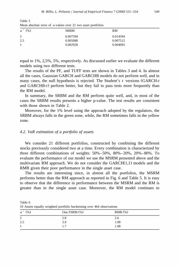
Fig. 7. One FRSM: backtesting VaR values for the equally weighted portfolio at different confidencelevel.


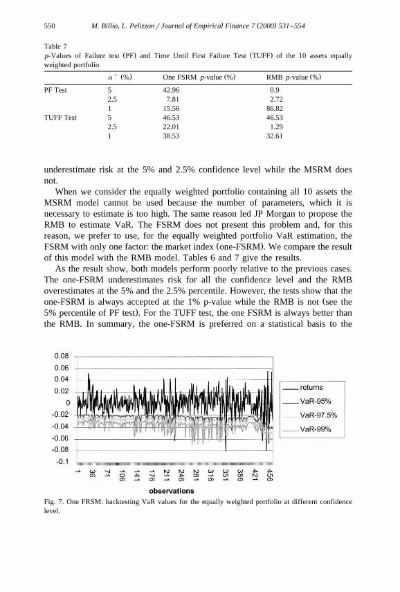
Fig. 8. RMB: backtesting VaR values for the equally weighted portfolio at different confidence level.

RMB. The one-FSRM could be easily improved by increasing the number offactors.

Furthermore, it is interesting to note the implications of the two models forVaR based capital requirements.9 It is evident from Figs. 7 and 8 that theone-FSRM is better than the RMB to capture quickly the changes in volatility ofthe returns. This implies that the former model requires a high capital allocationonly when the market is highly volatile and avoids high capital when marketvolatility returns to normality. In contrast, RMB always requires a high capitaleven when market volatility decreases.

Furthermore, it is interesting to observe that the average VaRs at the differentconfidence levels are: for the FSRM, 2.46%, 3.05% and 3.86% with standarddeviations of 0.62%, 0.77% and 0.89%, respectively; while, for the RMB theVaRs at the different confidence levels are on the average: 2.99%, 3.57% and4.23% with standard deviations 0.87%, 1.04% and 1.23%, respectively. Thismeans that the FSRM leads to a lower level of capital required and smallerrevision to required capital.

5. Conclusion

This paper has analysed the application of switching regime models to measur-ing VaR in order to account for a non-normal return distribution. Four different

9 In Jannuary 1996, the Basle Supervisory Commitee issued a Market Risk Ammendment to theŽ Ž ..1988 Accord Basle Commitee on Banking Supervision 1996 , specyfing a minimum capital

requirement based on bank internal models for market risks. This approach takes daily VaR calcula-tions from the bank’s own risk management system and applies a multiplier to arrive at a requiredcapital set-aside to cover market portfolio risk.


switching models are considered: SSRM, SRBM for one asset, MSRM for twoassets portfolio and the FSRM for an equally weighted portfolio containing 10assets. To illustrate the application of our approach we calculated the VaR for 10individual Italian stocks and for the MIB30 market index. We compared ourresults with those obtained from the variance–covariance RiskMetrics approach

Ž .and two versions of the GARCH 1,1 model.For portfolios with one and two assets the SRBM and MSRM perform well for

almost every percentile and every portfolio. In fact, the results are close to thetheoretical values and it does not seem that models persistently under or overestimate each level of confidence. The SRBM model always performs better thanthe SSRM and this means, as expected, that the link with the market is fundamen-tal for the estimation of equity risk.

The SRBM performs better than GARCH and GARCHB models. In fact theGARCH and GARCHB models do not work well as the number of exceptionsdeviates significantly from the theoretical values for almost all the stocks. Gener-ally, the values are higher than the theoretical ones for the Gaussian version andlower for the Student’s t version. This means that these models always underesti-

Ž . Ž .mate Gaussian or overestimate Student’s t risk.Ž .With regard to the RiskMetrics approach we considered two models: one RM

Ž .based on the variance estimation of the single asset and the other RMB wherethe risk of a single asset is determined by its beta with respect to the market index.The RM performs better that the RMB for all the portfolios. Moreover, RM andRMB usually overestimate the risk at the 5% and the 2.5% confidence levels, andunderestimate the risk at the 1% level. In other words, this approach does notreliably capture the risk of the extreme events. Comparing the RM results with theSRBM for one asset and with the MSRM for the two asset portfolio we find thatin most of the cases the SRBM and MSRM performs better than RM and RMB.These results are confirmed by two tests: the PF test and the TUFF test and by theapproach adopted by regulators for backtesting.

Finally, we estimate VaR for an equally weighted portfolio containing all 10stocks. We use the one-FSRM and the RMB in order to estimate VaR. Bothmodels performs poorly. However, the PF test and the TUFF test indicate that theone-FSRM is statistically preferable to the RMB model. This result is importantand suggests that, with a higher number of factors, the FSRM has the potential toprovide reliance estimates of market risk.

Acknowledgements

We gratefully acknowledge conversations with our supervisors, Alain Monfortand Stephen Schaefer, and help by Tiziana De Antoni. Pelizzon thanks ESRC forfinancial support.


References

Akgiray, V., Booth, G.G., 1988. Mixed diffusion jump process modelling of exchange rate movements.Review of Economics and Statistics 70, 631–637.

Ang, A., Bekaert, G., 1999. International asset allocation with time varying correlations. Mimeo,Graduate School of Business, Stanford University.

Billio, M., Pelizzon, L., 1997. Pricing option with switching regime volatility, Nota di Lavoro 97.07,Dipartimento di Scienze Economiche, University of Venice.

Bollerslev, T., Chou, R.Y., Kroner, K.F., 1992. ARCH modelling in finance. Journal of Econometrics52, 5–59.

Campbell, S.D., Li, C., 1999. Option pricing with unobserved and regime switching volatility, Mimeo,University of Pennsylvania.

Clark, P., 1973. A subordinated stochastic process with finite variance for speculative prices.Econometrica 41, 135–156.

Engel, C., Hamilton, J.D., 1990. Long Swings in the Dollar: are they in the data and do markets knowit? American Economic Review, 80.

Geman, H., Ane, T., 1996. Stochastic subordination. Risk 9, 146–149.´Goldfeld, S.M., Quandt, R.E., 1973. A Markov model for switching regressions. Journal of Economet-

rics 1, 3–15.Goldfeld, S.M., Quandt, R.E., 1975. Estimation in a disequilibrium model and the value of information.

Journal of Econometrics, 3.Gourieroux, C., 1992. Modeles ARCH et applications Financieres. Economica, Paris.´ ` `Hamilton, J.D., 1989. A new approach to the Economic Analysis of nonstationary time series and the

business cycle. Econometrica 57, 357–384.Hamilton, J.D., 1994. Time Series Analysis. Princeton Univ. Press.Hamilton, J.D., Susmel, R., 1994. Autoregressive conditional heteroskedasticity and changes in regime.

Journal of Econometrics 64, 307–333.Hsieh, D.A., 1988. The statistical properties of daily foreign exchange rates: 1974–1983. Journal of

International Economics 24, 129–145.Jeanne, O., Masson, P., 1999. Currency crises, sunspots and Markov switching regimes. Proceedings

FFM99 London.Khabie-Zeitoun, D., Salkin, G., Cristofides, N., 1999. Factor GARCH, regime switching and term

structure models. Proceedings FFM99 London.Kupiec, P.H., 1995. Techniques for verifying the accuracy of risk measurement models. The Journal of

Derivatives, 73–84.Linsmeier, T.J., Pearson, N.D., 1996. Risk Measurement: An introduction to Value at Risk, Working

Paper University of Illinois at Urbana-Champain.Longerstay, J., 1996. An improved methodology for measuring VaR. RiskMetrics Monitor Second

Quarter, J.P. Morgan.Mandelbrot, B., 1963. The variation of certain speculative prices. Journal of Business 36, 394–419.Meese, R.A., 1986. Testing for bubbles in exchange markets: a case of sparkling rates? Journal of

Political Economy 94, 345–373.Muller, U., Dacorogna, M., Davj, R., Olsen, R., Ward, J., 1993. Fractals and Intrinsic Time: A¨

Challenge to Econometricians. Olsen and Associates Publisher, Geneva, Swiss.Pagan, A.R., Schwert, G.W., 1990. Alternative models for conditional stock volatility. Journal of

Econometrics 45, 267–290.Phelan, M.J., 1995. Probability and statistics applied to the practice of financial risk management: the

case of JP Morgan’s RiskMetrics, Working Paper Wharton School.Quandt, R.E., 1958. The estimation of the parameters of a linear regression system obeying two

separate regimes. Journal of the American Statistical Association 53r284, 873–880.RiskMetrics, 1995. Technical Document, JP Morgan. New York, USA.


Rockinger, M., 1994. Regime switching: evidence for the French stock market, Mimeo HEC.Rogalski, R.J., Vinso, J.D., 1978. Empirical properties of foreign exchange rates. Journal of Interna-

tional Business Studies 9, 69–79.Turner, C.M., Startz, R., Nelson, C.R., 1989. A Markov model of heteroschedasticity, risk and learning

in the stock market. Journal of Financial Economics 25, 3–22.van Norden, S., Schaller, H., 1993. Regime Switching in Stock Market returns, Mimeo Bank of Canada

and Carleton University.

value-at-risk: a multivariate switching regime approachsmartquant.com/references/var/var2.pdf ·...

Documents