using normal curves - asq.qualitycampus.comasq.qualitycampus.com/guides/com_000_01130.pdf · area...

Using Normal Curves

Using Normal Curves introduces you to the normal curve. You also learn how to make predictions using the normal curve.

This course contains two lessons:

Lesson 1: What is Normal?

Lesson 1 reviews three characteristics of the normal curve: shape, central tendency and dispersion. You learn how to recognize a normal curve by examining its shape.

Lesson 2: Predicting with Normal Curves

Lesson 2 explains the use of normal curves to predict how much of a population meets specifications.

Page 24 Using Normal Curves

Terms Defined in the Glossary

• Normal Curve

• Parts Per Billion Defective (PPB)

• Parts Per Million Defective (PPM)

• Percent Defective

• Standard Normal Table

Using Normal Curves 5

Lesson 1: What is Normal?

Among the many types of distributions used in manufacturing, the normal distribution is the most widely used and studied. The normal distribution has long been used to describe errors in measurement. Although other distributions also occur in manufacturing, this course focuses on the normal distribution.

Characteristics of the Normal Distribution

The characteristics of shape, central tendency, and dispersion of the normal curve have some special properties that distinguish it from other curves.

1) Shape: The graph of the normal distribution is a bell-shaped curve with a single peak occurring at the mean. The normal curve has tails that extend indefinitely in both directions. The tails come closer and closer to the horizontal axis, but never actually touch it.

µ

Single Peak

Bell-shape

Tail Tail

Figure 34. Normal Curve


In order to determine if a population is normal, you can plot sample data and examine the shape of the emerging histogram. If the shape of the histogram appears bell-shaped, you assume that the population is normal. Let's take a look at some distributions that are not normal and identify what distinguishes them from normal distributions.

The following distribution is not normal because it has more than one peak. Remember, a normal distribution has only one peak occurring at the mean.

Figure 35. Bimodal Curve

The following distribution is not normal because it does not have tails and is not bell-shaped. A normal distribution is bell-shaped and has two tails extending indefinitely in both directions.

Figure 36. Uniform Curve

Looking at the shape of a curve gives you some idea about whether or not a distribution is normal. You can perform mathematical tests to check for normality.

Using Normal Curves Page 27

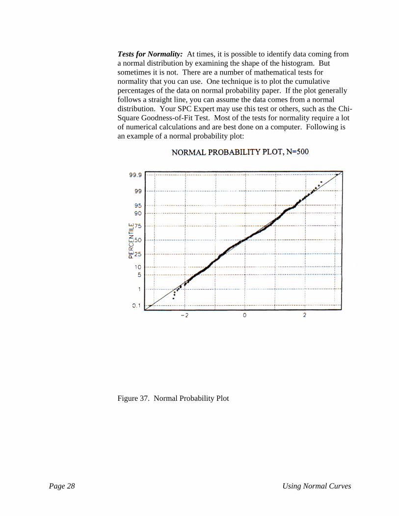
Tests for Normality: At times, it is possible to identify data coming from a normal distribution by examining the shape of the histogram. But sometimes it is not. There are a number of mathematical tests for normality that you can use. One technique is to plot the cumulative percentages of the data on normal probability paper. If the plot generally follows a straight line, you can assume the data comes from a normal distribution. Your SPC Expert may use this test or others, such as the Chi-Square Goodness-of-Fit Test. Most of the tests for normality require a lot of numerical calculations and are best done on a computer. Following is an example of a normal probability plot:

Figure 37. Normal Probability Plot


2) Central Tendency: The middle of the normal curve represents the center of the data, or the central tendency. It is known as the mean or µ. The peak of the curve is located at the mean. Normal curves are symmetrical about the mean. That is, if you divide the curve at the mean, both sections appear to be a mirror image of the other.

Figure 38. Normal Curve

Though the normal curve is symmetrical about the mean, not all distributions are symmetrical. For example, the following curve is lopsided and is not symmetrical about the mean.

Figure 39. Skewed Distribution

If you divided this curve at its mean, each section would not be a mirror image of the other.


x

Estimating the Mean: When using the normal distribution to model a population, you rarely know the mean, µ. Therefore, you estimate µ by using , the mean of the sample.

xTo calculate , you add all the individual values and divide by the total number of values. This can be expressed as:

x sum of all the individual values

=total number of values

Mathematically, this can be written with symbols as:

x

Σ x i=

n

where n is the sample size and Σ x i is the sum of the individual values; and each value is represented by x.

Example: For purposes of this calculation, a small sample size is used. Larger sample sizes are usually used when modeling a population. Here is a sample of measurements:

3 5 8 7 2 5 4 6

First, find the sum of all the individual values:

Σ xi = x1 + x2 + x3 + ………………..+ x8

= 3 + 5 + 8 + 7 + 2 + 5 + 4 + 6

= 40

The total number of values is 8; so n = 8. Therefore, the sample mean is:

x 40

8= 5 =

xRecall, the value of is the sample estimate of the population mean µ.


3) Dispersion: Although all normal curves are bell-shaped, their widths may vary. The dispersion or spread gives an indication of the width of the normal curve.

You measure dispersion in distances called standard deviations. Since you are working with the population, standard deviation is represented by σ (sigma). The greater the dispersion, the larger the standard deviation. The smaller the dispersion, the smaller the standard deviation.

Following are three normal curves that have the same mean, but different standard deviations.

Figure 40. Processes with Different Dispersion

The curve representing Process A, is wider than the other curves. Of the three processes, Process A has the largest standard deviation or σ.


Let's take a closer look at standard deviation. For Process D, both of the distances shown are one standard deviation from the mean.

Figure 41. One Standard Deviation for Process D

Here is another process with a normal distribution. The distances shown here are also one standard deviation from the mean.

Figure 42. One Standard Deviation for Process E

Yet these distances are much less than the distances shown for Process D. This is because the standard deviation for Process E is less than that of Process D.


No matter how wide or narrow the normal curve is, you can locate points on each side of the mean which are 1, 2, 3 or more standard deviations from the mean.

Figure 43. Standard Deviations

Example: Suppose you have a normal curve that has a mean of 70 and a standard deviation of 10.

Figure 44. Normal Curve. µ = 70, σ = 10

The points labeled 60 and 80 are one standard deviation from the mean. The points labeled 50 and 90 are two standard deviations from the mean. And the points labeled 40 and 100 are each three standard deviations from the mean.

Although the normal curve extends indefinitely in both directions, it appears to touch the axis at three standard deviations on each side of the mean. This is true for all normal curves.


Estimating Standard Deviation: Since you rarely know the value of the population standard deviation, σ, you can estimate it by using the sample standard deviation, s.

The formula for s is:

√ n - 1 Σ ( x i - x )

2 =s

xThe formula may look complicated, but the calculation is not that difficult with a small set of data. Using the data from the calculation, calculate s.

The sample data was:

3 5 8 7 2 5 4 6

Remember: The sample mean was calculated. It was 5.

Start with the numerator in the formula for s.

Σ ( x i - x )

2

xSTEP 1: For each value in the sample, calculate the distance between the

value and the mean, .

xx (x - )

3 (3 - 5) = -2

5 (5 - 5) = 0

8 (8 - 5) = 3

7 (7 - 5) = 2

2 (2 - 5) = -3

5 (5 - 5) = 0

4 (4 - 5) = -1

6 (6 - 5) = 1


( xi - x )

Σ ( x i - x ) 2

( xi - x ) 2STEP 2: Next, to calculate , multiply each number from STEP

1 by itself. STEP 2: Next, to calculate , multiply each number from STEP

1 by itself.

That is: That is:

The 2 is called aThe 2 is called a

It tells you to muIt tells you to mu

( xi - x ) 2 ( xi - x ) x ( xi - x )

-2 -2

0 0

3 3

2 2

-3 -3

0 0

-1 -1

1 1

STEP 3: The summation STEP 2.

STEP 3: The summation STEP 2.

Adding these values gives Adding these values gives

Using Normal Curves

=

( xi - x ) 2

n exponent. n exponent.

ltiply the number in parentheses by itself. ltiply the number in parentheses by itself.

(-2) x (-2) = 4 (-2) x (-2) = 4

(0) x (0) = 0 (0) x (0) = 0

(3) x (3) = 9 (3) x (3) = 9

(2) x (2) = 4 (2) x (2) = 4

(-3) x (-3) = 9 (-3) x (-3) = 9

(0) x (0) = 0 (0) x (0) = 0

(-1) x (-1) = 1 (-1) x (-1) = 1

(1) x (1) = 1 (1) x (1) = 1

symbol,Σ , tells you to add the results from symbol,Σ , tells you to add the results from

= 4 + 0 + 9 + 4 + 9 + 0 + 1 + 1 = 4 + 0 + 9 + 4 + 9 + 0 + 1 + 1

= 28 = 28

you 28, the value of the numerator. you 28, the value of the numerator.

Page 35

Next, calculate the denominator.

STEP 4: Take the number of values in the sample and subtract one.

Remember that the number of values in the sample is represented by n.

In this example, the sample size is 8. So, n - 1 = 7.

STEP 5: Divide the numerator by the denominator and take the square root of the result.

√ n 1 -Σ ( x i - x )

2

28

7 √ 4 = 2.0

So for this sample, the standard deviatiohow far the individual values vary from

For large sets of data, this calculation isof calculators and computers, it becomedeviation.

Page 36

=
√
n is 2.0. This te the mean.

very cumbersoms very easy to ge

Usi

=

lls us, on average,

e. With the use t the standard

ng Normal Curves

Using Normal Curves -- Activity 1

Purpose: To provide practice in identifying and describing characteristics of the normal distribution.

Instructions: Answer each of the following questions in the space provided.

1. List at least three characteristics that can be used to tell if a curve is normal.

A. ________________________________________

B. ________________________________________

C. ________________________________________

D. ________________________________________

E. ________________________________________


Use the following diagram to answer questions 2 - 4.

Figure 45. Normal Curves

2. Which of the following best describes these two normal curves?

A. They have the same mean but different standard deviations.

B. They have different means but the same standard deviations.

3. In Process A, a distance that is approximately three standard deviations away from the mean occurs at ____________________

4. Give an estimate for the value of the standard deviation for Process A. __________________

Hint: Use your answer from question 3.


Lesson 2: Predicting with Normal Curves

Lesson 2 shows how to use the normal curve in predicting the amount of parts that meet specifications. The predictions made in this unit assume you have a normally distributed population and estimates for µ and σ.

Area Under the Normal Curve

Lesson 1 showed how to find distances that are 1, 2, 3 or more standard deviations from the mean on a normal curve. This lesson shows how to find the area under the normal curve for those same distances.

The total area under any normal curve is equal to 1. Since the normal curve is symmetrical about its mean, the area on each side of the mean is .5. This is the same as saying that 50% of the area is on each side of the mean in a normal curve.

Figure 46. Area Under the Normal Curve

When the normal distribution models the population, 50% of the population is greater than the mean and 50% is less than the mean.

Now let's find the areas for 1, 2, 3 or more standard deviations on each side of the mean for a normal curve. To do this involves using a special normal curve, the standard normal distribution.


Standard Normal Distribution

The standard normal distribution has a mean of 0 and a standard deviation of 1. That is, µ= 0, and σ = 1. The curve looks like this:

Figure 47. Standard Normal Curve

Like all normal distributions, the curve appears to touch the axis at 3 standard deviations on each side of the mean. Since σ = 1, that would be at the values of +3 and -3.

Given a specific value, it is possible to find the area under the standard normal curve by using a standard normal table.


The Standard Normal Table: There are many formats used to display the standard normal table. Most standard statistical textbooks have a version of the standard normal table. The following table gives the area under the normal curve for a specified area.

Z: The value in this column indicates the number of standard deviations away from the mean.

Area D: The area less than – Z plus the area greater than +Z. Use this column to find the area outside the specification limits.

Area C: The area greater than +Z. Use this column to find the area outside a specification limit. Because the normal curve is a mirror image around its mean, this is also the area less than – Z.

Area B: The area between –Z and +Z values. It is accurate to the number of decimal places shown. Due to rounding, it will not always be twice the value shown in Area A. Use this column to calculate yield or the amount of product that meets specifications.

Area A: The area between the mean and the +Z value. It can also be the area between the mean and -Z since the normal curve is a mirror image around its mean.


Z Area A Area B Area C Area D 0.1 .0398 .0797 .4602 .9203 0.2 .0793 .1585 .4207 .8415 0.3 .1179 .2358 .3821 .7642 0.4 .1554 .3108 .3446 .6892 0.5 .1915 .3829 .3085 .6171 0.6 .2257 .4515 .2743 .5485 0.7 .2580 .5161 .2420 .4839 0.8 .2881 .5763 .2119 .4237 0.9 .3159 .6319 .1841 .3681 1.0 .341345 .6827 .158655 .3173 1.1 .3643 .7287 .1357 .2713 1.2 .3849 .7699 .1151 .2301 1.3 .4032 .8064 .0968 .1936 1.4 .4192 .8385 .0808 .1615 1.5 .4332 .8664 .0668 .1336 1.6 .4452 .8904 .0548 .1096 1.7 .4554 .9109 .0446 .0891 1.8 .4641 .9281 .0359 .0719 1.9 .4713 .9426 .0287 .0574 2.0 .47725 .9545 .02275 .0455 2.1 .4821 .9643 .0179 .0357 2.2 .4861 .9722 .0139 .0288 2.3 .4893 .9786 .0107 .0214 2.4 .4918 .9836 .0082 .0164 2.5 .4938 .9876 .0062 .0124 2.6 .4953 .9907 .0047 .0083 2.7 .4965 .9931 .0035 .0069 2.8 .4974 .9949 .0026 .0051 2.9 .4981 .9963 .0019 .0037 3.0 .49865 .9973 .00135 .0027 3.1 .4990 .9981 .0010 .0019 3.2 .4993 .9986 .0007 .0014 3.3 .4995 .9990 .0005 .0010 3.4 .4997 .9993 .0003 .0007 3.5 .4998 .9995 .0002 .0005 3.6 .49984 .9997 .00016 .0003 3.7 .4999 .9998 .0001 .0002 3.8 .49993 .99986 .0007 .00014 3.9 .49995 .9999 .00005 .0001 4.0 .49997 .999937 .00003 .000063 4.5 .4999966 .9999932 .0000034 .0000068 5.0 .4999997 .99999943 .0000003 .00000057 6.0 .499999999 .999999998 .000000001 .000000002


Using the table, it is easy to find the area under the normal curve for specific values or distances from the mean. Let's see how:

Find the area from the mean to a value that is one standard deviation above the mean. This area is shown below:

Figure 48. Area For One Standard Deviation

Look under the first column in the table for the value of Z that is 1.0. Use the column that gives the desired area. In this case, you want the area listed under Area A. This value is .341345.

Z Area A Area B Area C Area D

1.0 .341345 .6827 .158655 .3173

Since the total area is 1, .341345 represents 34.1345% of the total area under the normal curve. With the normal curve being symmetrical about its mean, the same amount of area is also between the mean and one standard deviation below the mean. Therefore, the total area from -1 to +1 is:

.341345 + .341345 = .68269


When rounded to 4 decimal places, .6827 is the value found for Z = 1.0 in the column labeled AREA B. Thus, 68.27% of the area under the standard normal curve is found within one standard deviation on each side of the mean.

Figure 49. Area Within One Standard Deviation of the Mean

Similarly, you can do this for any value. The following diagram shows the percentage of the area under the standard normal curve for distances that are 1, 2, 3, 4, 5 and 6 standard deviations on each side of the mean.

Figure 50. Area Under Standard Normal Curve


Other Normal Curves

It is possible to relate any normal curve to the standard normal distribution. This makes it very easy to apply the normal curve to many different applications. The areas specified for the standard normal curve are the same for any normal curve. For example, suppose that a population had a mean, µ= 70, a standard deviation σ = 10, and was normally distributed. What percentage of the area would be between the values of 60 and 80? Examine the following diagram:

Figure 51. Normal Curve. µ= 70, σ= 10

Notice, that the points 60 and 80 are each one standard deviation on each side of the mean, 70. The area under this curve is the same as the area under the standard curve between the values of -1 and +1. Using the table, this value is .6827. This is a special property of all normal curves. Any normal curve can be transformed to the standard normal curve.

x - µ

You can use this method with all normal curves to find specific areas. For any given value, just calculate how many standard deviations the value is from the mean. This can be done with a simple formula:

Z

σ=

The result is called a Z score which is used with the standard normal table to find the needed area.

x When applying this formula to populations, you rarely know the values of µ and σ, so use the sample estimates, and s. In this case, the formula would be:

x - x

s =Z


Let's look at applying this concept to the following example involving the length of bolts after variation was reduced.

Example: A bolt manufacturer produces bolts where one critical parameter is the length of the bolts. To meet customer requirements, the specification limits are 22 mm and 28 mm. Bolts shorter than 22 mm are scrap. Bolts longer than 28 mm require rework--cutting them to the required length. The sample estimates for the mean is 25 mm and the standard deviation is 1.0 mm. The control charts for this process are stable and the histogram followed the shape of a normal curve. The following questions need to be answered:

a) What is the yield of this process?

b) How much rework is required?

First, the yield is defined as the percentage of product meeting specifications without rework. This is the percentage of bolts that are between 22 mm and 28 mm in length. The area between the spec limits in this diagram represents the yield:

Figure 52. Normal Curve. µ ≈ 25, σ ≈ 1 (using estimates from sample)


You need to know the total area under this normal curve between the LSL of 22 and the USL of 28. This requires that the Z score for each spec limit is calculated.

For the USL: 28 - 25

1.03.0 =

=Zusl

For the LSL:

22 - 25

1.0-3.0=

=Zlsl

The yield for this process is determined by finding the area under the standard normal curve between the Z scores of -3 and +3. Look at the Standard Normal Table in the row corresponding to +3, under the column Area B. The area is .9973, so the yield is 99.73%.

How much rework is required? This is the percentage of bolts that have a length greater than 28 mm. On the normal curve this is shown as:

Figure 53. Amount of Bolts Requiring Rework

Find the area outside the USL. The Z score for the USL of 28 was already calculated, it was +3. To find the area greater than +3 for the standard normal curve, use column Area C in the table. The value is .0013. Therefore, .13% of the parts will need to be reworked. For small percentages like .13%, it is easier to express this in terms of parts per million or ppm.


Parts Per Million (ppm): To convert a percentage to parts per million, move the decimal point 4 places to the right. For example:

.13% is equivalent to 1300 ppm

In the previous example, 1300 represents the number of bolts out of one million that need to be reworked. Another way of saying this; for every one million bolts produced, 1300 bolts need to be reworked.

PPM is just another way of expressing a ratio;

1300 1,000,000

= .0013

and to convert to a percentage, multiply by 100,

.0013 x 100 = .13 %

So, .13% is equivalent to saying 1300 ppm.

Parts Per Billion (ppb): When quality reaches a certain level, expressing the amount of parts that do not meet spec in ppm is awkward. You can then convert the decimal, percentage, or ppm to ppb.

Let's take a process that has the area outside the specs to be .000000002.

To represent the decimal as a percentage, you multiply the decimal by 100:

.000000002 x 100 = .0000002 %

To represent the decimal as parts per million, you multiply the decimal by 1,000,000.

.000000002 x 1,000,000 = .002 ppm

To represent the decimal as parts per billion, you multiply the decimal by 1,000,000,000.

.000000002 x 1,000,000,000 = 2 ppb

And when the quality level gets even better, you could use parts per trillion!


Summary: In this lesson you learned how to use a mathematical model like the normal distribution to help predict yield and the amount of product that does not meet specifications. Even though the normal distribution cannot be used for all populations, the method of fitting a mathematical model to data and then using that model for prediction is very useful.


Using Normal Curves -- Activity 2

Purpose: Use the normal curve to predict the amount of parts that meet specifications and express the answer as a decimal, percentage or ppm.

Instructions: Answer each of the following questions. Use the standard normal table when needed.

1. Complete the following table by filling in the columns for percentage and ppm for each decimal value shown.

DECIMAL Percentage PPM .0357

.0027

.00006

.0000034

.4554


Use this diagram to answer questions 2 and 3. In this process, µ= 30 and σ = 5 . The distribution

is normal.

Figure 54. Normal Curve. µ= 30, σ = 5

2. Find the area that is outside the specifications limits. The specification limits are 20 and 40. Express your answer as a decimal, a percentage, and in terms of ppm.

3. Express the yield, the area inside the specification limits, as a percentage.


4. The mean for the process shifts to a new value of 35. The standard deviation does not change, σ = 5. The new process is shown in the diagram below. The specification limits are 20 and 40.

Figure 55. Normal Curve. µ = 35, σ = 5

For this process, what is the amount of area that is outside the specifications limits now? Express your answer in parts per million (ppm).


using normal curves - asq.qualitycampus.comasq.qualitycampus.com/guides/com_000_01130.pdf · area...

Documents