using aerial photography and geographic …...practical paper using aerial photography and...
TRANSCRIPT
Practical Paper
Using Aerial Photography and GeographicInformation Systems to Develop Databases forPesticide EvaluationsJames L. Smith, Jesse A. Logan, and Timothy G. GregoireDepartment of Forestry, Virginia Tech, Blacksburg, VA 24061-0324
ABSTRACT: An example of the construction of a spatial and attribute database using aerial photography and GIS isdescribed. Two vegetative layers on two large experimental plots were interpreted on t~e aerial photo?Caphs ,anddigitized. A theme of trap locations was generated and linked to the results of 16 tr,appll~g days sp~nmng penodsbefore and after the application of a pesticide. The GIS was used to calculate val,ues which will be used In a later stU?yto model the effects of the pesticide on the small-mammal community. Both aenal ph?~ography a~d GIS show promisefor improving the efficiency with which data can be gathered and processed for pestiCide evaluahons.
INTRODUCTION AND BACKGROUND
O NE OF THE IMPORTANT TASKS of the U.S. EnvironmentalProtection Agency and other environmental agencies i!i to
evaluate the effect of pesticides on non-targeted floral and faunalpopulations in the treated areas. The analytic techniques neededto perform these assessments are often complex, with intensiveand extensive information requirements, which J;lakes the evaluation process slow and expensive. The technologies of remotesensing and geographic information systems offer promise forstreamlining this evaluation process. There has been ampleprecedent in the literature for using these new technologies tomonitor and evaluate wildlife populations (Agee and Stitt, 1989;Donovan et al., 1987; Heinen and Lyon, 1989; Johnson, 1990;Stutheit, 1989).
A project was initiated to examine the use of aerial photography and GIS for developing spatial databases which could beused in the pesticide evaluation process. In an earlier study ofthe pesticide methamatiphos, which provided the basis for thisproject, four treatment and two control plots were establishedin northeastern Colorado. The pesticide was applied to each ofthe four treatment plots, with two plots receiving a single application, and two a second application. The pesticide was targeted at insect populations, but the interest was on the effectof the pesticide on the remaining small-mammal populationswhich prey on the insects. A small-mammal trap grid was established on each plot, and the results of four trap periods offour days each were recorded. One trap period took place priorto the application of the pesticide, and three following the application over a specified time interval. To analyze this data set,a way to map the vegetation cover efficiently, and a way tocorrelate this vegetation information with the trapping results,was needed.
The power of a GIS resides in its ability to associate locationsand characteristics, and its ability to cross-reference differenttypes of spatial information. We needed both of these abilitiesin this endeavor. Our first need was to quantitatively characterize the vegetation in the vicinity of each trap by methods ofneighborhood analysis. Because different faunal species traveldifferent distances for food, water, and shelter (varying homerange sizes), and these distances were largely unknown in theseareas, it was necessary to characterize the vegetation withinvarying neighborhood sizes to help modelers determine the be-
PHOTOGRAMMETRIC ENGINEERING & REMOTE SENSING,
Vol. 58, No. 10, October 1992, pp. 1447-1452.
havior of the species encountered. Clearly, this required thatthe analyses be easily repeated. Further, because trap locationsand vegetation information were stored as separate themes, allthese analyses would require Boolean combinations of somesort.
The objective of this paper is to describe how aerial photography and GIS were used to develop data sets for use in, assessing the effect of a pesticide on a small-mammal populatlOn.This situation is similar to more traditional uses of GIS in thatit is a spatially oriented problem, with all the requirements andlimitations that implies. However, it is somewhat different fromprevious GIS applications because the data set was specificallydesigned and developed for analysis only. There is not otherwise any need to map experimental plots, except as the m~p
ping applies to the spatial analyses performed. We emphaSizethat the spatial data sets developed in this study were constructed with different objectives in mind than, say, a subdivision or a forest stand database.
METHODS
PLOT DESCRIPTION AND PHOTOINTERPRETATION
Six experimental plots were established in the Colorado PlainsExperimental Range in northeastern Colorado. Each plot was225 metres square, or 5.06 hectares (12.5 acres). This area is anative shortgrass prairie, consisting predominantly of buffalograss (Buchloe dactyloides), blue grama (Boutela gracilis), several midgrasses, and similar species (Stevens, 1989). Taller shrubsor small trees were also present on the plots in highly variableamounts. The topography was flat to gently rolling, and theelevation was approximately 1500 metres. Soils are shallow, sandyloams, and the rainfall was around 5 centimetres per year.
The four corners of each plot were targeted for precise aerialidentification. Because of budgetary and time restrictions, twoof the six plots were selected for examination in this study. Thisselection was based on aerial photo coverage and overall photoquality. Aerial photography was acquired of each plot just following plot establishment using a 9-inch camera carrying normal color film during a period of full-leaf cover. Positives wereenlarged approximately 3 times and printed at a scale of about1:700. Print contrast was reduced by the enlarging and printingprocesses, and scratches and marks on the originals marred the
0099-1112/92/5810-1447$03.00/0©1992 American Society for Photogrammetry
and Remote Sensing
1448 PHOTOGRAMMETRIC ENGINEERING & REMOTE SENSING, 1992
prints. Despite these defects, these photos were used in thisproject. The very large scale was necessary for the proposedphotointerpretation and mapping objectives. Because thesephotographs were acquired during time periods spanned by thetrapping sessions, there was no time lag between field effortsand the subsequent photointerpreted information. Further, thegoal of the interpretation process was relatively simple - thelocation and delineation of shrubs - which should be accurateand consistent on these slightly degraded images.
The enlarged print for each of two plots was monoscopicallyinterpreted using a 5 x monocular magnifier. Because stereocoverage was not available, monoscopic interpretation methodswere utilized. A clear mylar overlay was attached to each print,and all interpreted results were noted on these overlays. Theintent was to map the location of individual shrubby or woodycrowns, and the boundaries of each crown where possible. Although the grass species comprise the majority of the groundcover, it was the woody shrubs which are thought to provideshelter for most activities of the small-mammals. Thus, theirlocation and extent are of primary importance when describinghabitat quality.
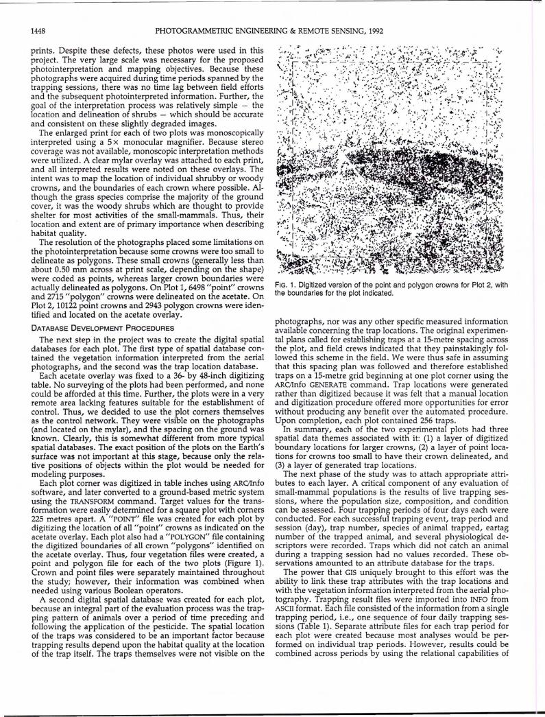
The resolution of the photographs placed some limitations onthe photointerpretation because some crowns were too small todelineate as polygons. These small crowns (generally less thanabout 0.50 mm across at print scale, depending on the shape)were coded as points, whereas larger crown boundaries wereactually delineated as polygons. On Plot 1, 6498 "point" crownsand 2715 "polygon" crowns were delineated on the acetate. OnPlot 2, 10122 point crowns and 2943 polygon crowns were identified and located on the acetate overlay.
DATABASE DEVELOPMENT PROCEDURES
The next step in the project was to create the digital spatialdatabases for each plot. The first type of spatial database contained the vegetation information interpreted from the aerialphotographs, and the second was the trap location database.
Each acetate overlay was fixed to a 36- by 48-inch digitizingtable. No surveying of the plots had been performed, and nonecould be afforded at this time. Further, the plots were in a veryremote area lacking features suitable for the establishment ofcontrol. Thus, we decided to use the plot corners themselvesas the control network. They were visible on the photographs(and located on the mylar), and the spacing on the ground wasknown. Clearly, this is somewhat different from more typicalspatial databases. The exact position of the plots on the Earth'ssurface was not important at this stage, because only the relative positions of objects within the plot would be needed formodeling purposes.
Each plot corner was digitized in table inches using ARC/lnfosoftware, and later converted to a ground-based metric systemusing the TRANSFORM command. Target values for the transformation were easily determined for a square plot with corners225 metres apart. A "poINT" file was created for each plot bydigitizing the location of all "point" crowns as indicated on theacetate overlay. Each plot also had a "POLYGON" file containingthe digitized boundaries of all crown "polygons" identified onthe acetate overlay. Thus, four vegetation files were created, apoint and polygon file for each of the two plots (Figure 1).Crown and point files were separately maintained throughoutthe study; however, their information was combined whenneeded using various Boolean operators.
A second digital spatial database was created for each plot,because an integral part of the evaluation process was the trapping pattern of animals over a period of time preceding andfollowing the application of the pesticide. The spatial locationof the traps was considered to be an important factor becausetrapping results depend upon the habitat quality at the locationof the trap itself. The traps themselves were not visible on the
FIG. 1. Digitized version of the point and polygon crowns for Plot 2, withthe boundaries for the plot indicated.
photographs, nor was any other specific measured informationavailable concerning the trap locations. The original experimental plans called for establishing traps at a IS-metre spacing acrossthe plot, and field crews indicated that they painstakingly followed this scheme in the field. We were thus safe in assumingthat this spacing plan was followed and therefore establishedtraps on a IS-metre grid beginning at one plot corner using theARC/lnfo GENERATE command. Trap locations were generatedrather than digitized because it was felt that a manual locationand digitization procedure offered more opportunities for errorwithout producing any benefit over the automated procedure.Upon completion, each plot contained 256 traps.
In summary, each of the two experimental plots had threespatial data themes associated with it: (1) a layer of digitizedboundary locations for larger crowns, (2) a layer of point locations for crowns too small to have their crown delineated, and(3) a layer of generated trap locations.
The next phase of the study was to attach appropriate attributes to each layer. A critical component of any evaluation ofsmall-mammal populations is the results of live trapping sessions, where the population size, composition, and conditioncan be assessed. Four trapping periods of four days each wereconducted. For each successful trapping event, trap period andsession (day), trap number, species of animal trapped, eartagnumber of the trapped animal, and several physiological descriptors were recorded. Traps which did not catch an animalduring a trapping session had no values recorded. These observations amounted to an attribute database for the traps.
The power that GIS uniquely brought to this effort was theability to link these trap attributes with the trap locations andwith the vegetation information interpreted from the aerial photography. Trapping result files were imported into INFO fromASCII format. Each file consisted of the information from a singletrapping period, i.e., one sequence of four daily trapping sessions (Table 1). Separate attribute files for each trap period foreach plot were created because most analyses would be performed on individual trap periods. However, results could becombined across periods by using the relational capabilities of
-
DATABASES FOR PESTICIDE EVALUATIONS 1449
INFO (or DBASE on pcARC). Because the trapping results werethe trap attributes of interest, and we wanted separate databases for the four trap periods, it was necessary to make fourcopies of the trap location spatial database for each plot, onefor each of the attribute data sets. Once these copies had beenmade, the JOINITEM command was used to permanently link atrap location layer to an appropriate set of trapping results, andthe process was repeated until all trap periods were spatiallyreferenced.
The databases were now complete. The data base for each ofthe two plots consisted of six themes of information. Themes 1and 2 were the vegetation location information interpreted fromthe aerial photographs. The linked attributes for these two layers were the standard values computed by ARClInfo, namely,the area and perimeter of the polygon crowns, and the area andperimeter of the point crowns. Themes 3 to 6 were the four traplocation databases, one each for the four trapping periods. Thelinked attributes for these layers were the trapping results previously described. Note again that it is beyond the scope of thispaper to present the results of the mammal evaluations, although some uses of the GIS in this regard will be briefly described.
SPATIAL ANALYSES
The databases were created for purposes of spatial analysis.Although there was no "mapping" intent in a display sense,we will later describe display products which we believe mayhelpful to the modelers. We discuss in this section how thedatabases were used to calculate values that could be used inan assessment of a faunal population.
Within ARClInfo, the BUFFER command was used to generatecircular proximity zones around each trap location with radii 1metre, 2 metres,S metres, and 7.5 metres. Each zone size wasmaintained as a separate polygon theme in the corporate database. Each zone size theme was then combined with the pointand polygon vegetation themes using the UNION command.This produced new themes which contained all point crownswithin the critical distance, and all crowns or crown portionswithin the specified zone size. Because there were two plotsand four zone sizes, this effort was made more efficient throughthe use of macros developed in the AML facility.
Several numerical descriptors were calculated for each trapusing functions available within ARClInfo. First, the total crownarea within the specified distances was computed by simplysumming the crown areas (as automatically calculated by ARC!Info) in the overlaid files. In order to estimate total crown coverage, we needed to account for the crown area occupied bypoint crowns. These crowns were too small to resolve on thephotography, but they occupy finite area on the ground.
We assumed that the area of individual point crowns wasequal to one-half of the average area of the 150 smallest polygoncrowns (separately done for each plot), then multiplied thisvalue by the number of point crowns to estimate total pointcrown area for each of the two plots. By adding point and polygon crown area, we estimate total woody crown cover withindifferent distances of the trap location. Within each proximityzone, the total number of interpreted point and polygon crownswas tallied and added to the database. This was considered tobe a measure of the total number of stems within specifieddistances of each trap. The distance from each trap location tothe nearest point crown, and the distance from each trap to thenearest crown boundary are, were computed using the NEARcommand within ARClInfo. Although the modelers may identifyother values to be computed using the databases we developed,our plan was complete (Table 2). Note that these calculatedvalues could be linked to the trap history results previouslydiscussed using the relational capabilities of INFO or DBASE. Thepros and cons of this effort will be discussed in a later section.
TABLE 1. EXAMPLE OF THE TRAP HISTORY DATABASE FOR TRAPS 1233 IN PLOT 2 FOR DAYS 1 AND 2 OF THE PRE-TREATMENT TRAPPING
PERIOD.
DAY 1 DAY 2
Weight TagTrap Tag # Species' Sex Age' (grams) # Species Sex Age Weight
12 1,306 PEMA M 1 23.000 0 0 0.000013 0 0 0.0000 0 0 0.000014 0 0 0.0000 0 0 0.000015 1,304 PEMA F 3 15.0000 0 0 0.000016 1,303 PEMA M 1 16.0000 0 0 0.000017 0 0 0.0000 0 0 0.000018 0 0 0.0000 1,318 REMO F 1 12.000019 0 0 0.0000 0 0 0.000020 0 0 0.0000 0 0 0.000021 0 0 0.0000 0 0 0.000022 0 0 0.0000 0 0 0.000023 0 0 0.0000 0 0 0.000024 0 0 0.0000 a a 0.000025 0 0 0.0000 0 0 0.000026 a a 0.0000 a a 0.000027 0 0 0.0000 0 0 0.000028 a a 0.0000 a 0 0.000029 0 0 0.0000 a 0 0.000030 0 0 0.0000 0 0 0.000031 a a 0.0000 a 0 0.000032 a 0 0.0000 a 0 0.000033 1,307 PEMA F 3 13.0000 1,319 PEHI M 1 50.0000
1 PEMA - Peromyscus maniculatus; REMO - Reithrodontomys mon-tanus; PEHI - Perognathus hispidus, 1 = Juvenile; 2 - Subadult; 3 - Adult
As we progressed through the database development process,we began to see other GIS "products" that might be useful tothe modeling process. These additional items were displayproducts created by manipulating the trap history databases, orby merging the various spatial themes and the trap histories.These images of the data are important because in a complexmodeling situation a greater understanding of the relationshipsbetween variables may be discerned with pictures than withraw numbers or statistics.
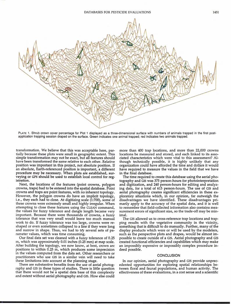
The first type of display product consisted of a trap locationmap, with the various traps labeled with text or different symbols according to important attributes in the trap history database, such as species trapped, or number of animals trappedover the period. This gave a strong indication of the spatialdistribution of the trap results. The second type of display wasa composite map of the two vegetation layers (point and polygon) and the trap locations labeled by attributes which helpedmodelers correlate trap results with vegetative composition. Finally, a third display was a three-dimensional view of the percent vegetative cover of the two plots, with the trap resultsdraped over this surface. This was a capability unique to GIS,and our procedure requires further explanation.
We took a simplistic approach to the creation of the threedimensional crown cover surface because the surface would beused only for viewing, not for calculating other values as isoften done with topographic surfaces. Our approach was to usecrown closure percentages computed from circular 7.5-m proximity zones and assume that they were the cell value for square15-m cells centered on each trap location. This became a simpleraster data set suitable for creating three-dimensional surfaceviews.
We decided to use the IDRISI package for these views for tworeasons: (1) IDRISI uses a file structure that could be easily created, and (2) IDRISI was an inexpensive and widely availablepackage that was more likely to be obtained off-site if local
1450 PHOTOGRAMMETRIC ENGINEERING & REMOTE SENSING, 1992
TABLE 2. EXAMPLES OF THE VALUES CALCULATED WITHIN THE G.IS FOR TRAPS 12-33 IN PLOT 2.
Number and Area of Crownswithin the Specified Distance of Each Trip
1.0 Metre 2.0 Metres 5.0 Metres 7.5 Metres Metres MetresRadius Radiius Radius Radius to to
Nearest NearestArea Area Area Area Point Polygon
Trap Num (M2) Num (M2) Num (W) Num (M2) Crown Crown
12 0 0.0000 0 0.0000 7 0.7466 14 1.7270 3.4 6.113 0 0.0000 0 0.0000 2 0.0517 16 3.1405 3.5 4.414 1 0.1672 2 0.3345 6 0.7207 24 3.7365 0.9 3.215 0 0.0000 1 0.1672 4 0.6690 17 2.5636 1.9 4.716 0 0.0000 1 0.4430 5 1.1120 17 3.3845 3.7 1.017 1 0.0259 4 0.1866 14 1.7176 34 4.6777 0.8 1.318 1 0.0259 3 0.3119 12 0.5447 24 1.3024 0.5 1.119 0 0.0000 1 0.0259 7 0.1811 23 0.7874 1.6 7.120 1 0.2150 2 0.2439 10 0.4508 31 1.1492 1.3 2.421 0 0.0000 3 0.0776 22 0.5691 41 1.3130 1.5 2.922 2 0.3130 2 0.7600 10 0.9670 22 3.6429 2.2 0.323 2 0.1610 4 1.2179 20 1.6318 46 7.6393 1.5 0.624 1 0.1860 2 0.2119 15 0.5482 47 4.7903 1.9 0.225 2 0.0869 5 0.2107 24 0.7022 45 3.2355 0.5 0.026 0 0.0000 0 0.0000 1 0.0259 8 0.6336 2.2 4.127 0 0.0000 1 0.4260 5 0.5295 9 0.9061 2.3 1.328 0 0.0000 1 0.5280 7 0.6832 23 2.1682 2.1 1.129 2 0.1930 3 0.6380 8 0.7673 26 1.9756 3.9 0.430 0 0.0000 0 0.0000 2 0.0517 6 0.5345 3.6 5.531 0 0.0000 1 0.0190 3 0.0707 13 2.1992 2.8 1.932 0 0.0000 1 0.0610 4 0.4214 15 4.4901 3.4 1.833 0 0.0000 1 0.0780 9 1.1332 21 2.9720 2.7 1.8
personnel want to view the results. We found the initial resultsunsatisfactory because of the large cell size. There was littlevariation in the surface, and it was very blocky in appearance.
We recreated the crown closure surface at a 5-m resolutionby first creating a 5-metre grid using the GENERATE commandof ARClInfo, and using the BUFFER command to develop 2.5metre radius proximity zones. We then overlaid this grid overthe point and polygon crown themes, and computed the crowncover percentage in the proximity zone as described above. Thisraster file was imported into lORISI and perspective plots weregenerated. The views generated from the 5-metre cell data wereconsidered to be acceptable and helpful by the modelers. Various trap history files were also linked to the lORISI images throughQUATIRO and draped over the crown cover surface. An exampleis presented in Plate 1.
DISCUSSION
We fulfilled the principal objective of describing how aerialphotography and GIS were used to construct databases designed for use in evaluating a small-mammal population following the application of a pesticide. It is relevant and importantto discuss what we learned about the use of GIS and aerialphotography in this context for the benefit of those who perform similar tasks in the future.
Several problems or difficulties were encountered during thecourse of the project. These accrue from imprecision in the spatial data sets, which creates imprecision in the values computedwith it in order to assess the small-mammal population. Remember, it is the small mammal assessment that is the goal,not the maps or the attributes. In t~s study, database qualitydepended upon the characteristics of the aerial photographs,the skill and effort of the photointerpreters, the digitizing process,and the algorithms used to process the raw data.
The first potential source of spatial inaccuracies was associated with the aerial photography and photointerpretation. Theaerial photography used in this project was of relatively poor
quality. The original positives were scratched, and appeared tobe slightly overexposed. When enlarged and printed, theseproblems were exacerbated. Thus, although the objective of theinterpretation was the simple identification of shrubby or woodyvegetation, there were undoubtedly some errors made by theinterpreters. It is well known that "real" crowns are often missedby photointerpreters, and that "false" crowns are identified andmapped (Needham and Smith, 1987). Although it was likelythat this problem was minimal in this project, we always urgeall who pursue similar aims to use the very best quality photographs available. Photointerpretation accuracy can presentsignificant problems as mapping objectives become more complex.
Besides image quality, image geometry could have createdproblems at these large scales in some situations. Because themapping was performed monoscopically, image displacementcould have been a significant degrading factor on the planimetric accuracy of the spatial data. However, the topographywas generally flat, so even at these low flying altitudes displacement should not be a measureable problem in this project.Although we believe that the quality of the photointerpretedvegetation overlays was acceptable for this project, no formalaccuracy assessment was performed. Clearly, the vegetationoverlays contain mapping errors which will have some impacton the results, although again we believe that this impact wasvery minimal. Future researchers should consider the importance of photographic properties if images are going to serve asthe major source of spatial information.
The digitizing procedure and the processing algorithms alsocreated some difficulties for future researchers to take note of.The first step in the digitizing procedure was to register themap to some ground measuring system. Because a predse Earthreference was not necessary in this project, we used the plotcomers and TRANSFORM command as previously described. Weacknowledge that this is not the most precise procedure forground referencing because this command uses a simple affine
-
DATABASES FOR PESTICIDE EVALUATIONS 1451
PLATE 1. Shrub crown cover percentage for Plot 1 displayed as a three-dimensional surface with numbers of animals trapped in the first postapplication trapping session draped on the surface. Green indicates one animal trapped; red indicates two animals trapped.
transformation. We believe that this was acceptable here, partially because these plots were small in geographic extent. Thissimple transformation may not be exact, but all features shouldhave been transformed the same relative to each other. Relativeposition was important in this project, not absolute position. Ifan absolute, Earth-referenced position is important, a differentprocedure may be necessary. When plots are established, surveying or GPS should be used to establish local control for registration.
Next, the locations of the features (point crowns, polygoncrowns, traps) had to be entered into the spatial database. Pointcrowns and traps are point features, with no inherent topology.However, the polygon crowns do have an implicit topology,Le., they each had to close. At digitizing scale (1:700), some ofthese crowns were extremely small and highly irregular. Whenattempting to close these features using the CLEAN command,the values for fuzzy tolerance and dangle length became veryimportant. Because there were thousands of crowns, a fuzzytolerance that was very small would leave too much manualwork to do. If fuzzy tolerance was too large, crowns were reshaped or even sometimes collapsed to a line if they were longand narrow in shape. Thus, we had to try several sets of parameter values, which was time consuming.
Our final data set was cleaned with a fuzzy tolerance of 0.25m, which was approximately 0.01 inches (0.25 rom) at map scale.After building the topology, we now know, at best, crown arcpositions to within 0.25 m, which produces some imprecisionin the values computed from the data set. Other researchers orpractitioners who use GIS in a similar vein will need to takethese limitations into account at the planning stage.
There are substantive benefits from the use of aerial photography and GIS in these types of studies. There is little questionthat there would not be a spatial data base of this complexityand extent without aerial photography and GIS. How else could
more than 400 trap locations, and more than 22,000 crownslocations be measured and stored, and each linked to its associated characteristics which were vital to this assessment? Although technically possible, it is highly unlikely that anyorganization could have afforded the time and dollars it wouldhave required to measure the values in the field that we havein the final database.
The time required to create this database using the aerial photography and GIS was 375 person-hours for photointerpretationand digitization, and 240 person-hours for editing and analyzing data, for a total of 615 person-hours. The use of GIS andaerial photography creates significant efficiencies in these exploratory situations which, in our opinion, far outweigh thedisadvantages we have identified. These disadvantages primarily apply to the accuracy of the spatial data, and it is wellto remember that field-collected information also contains measurement errors of significant size, so the trade-off may be minimal.
The GIS allowed us to cross-reference trap locations and trapping results with the vegetative community in the vicinity,something that is difficult to do manually. Further, many of thedisplay products which were or will be used by the modelers,such as the perspective plots and drapes, would be almost impossible to create outside of a GIS. Aerial photography and GIScreated functional efficiencies and capabilities which may makean impossibly expensive or impossibly complex procedure indeed possible.
CONCLUSION
In our opinion, aerial photography and GIS provide unprecedented opportunities for exploring spatial relationships between floral and faunal populations, and human activity. Theeffectiveness of these evaluations, in a cost sense and a scientific
1452 PHOTOGRAMMETRIC ENGINEERING & REMOTE SENSING, 1992
sense, can be enhanced through the use of these tools, if theyare well understood and well utilized.
ACKNOWLEDGMENT
Although the research described in this article has been fundedwholly or in part by U.S. Environmental Protection Agencyagreement CR-817661-01-0 to Virginia Tech, it has not been subjected to the Agency's review and therefore does not necessarilyreflect the views of the Agency, and no official endorsementshould be enferred.
REFERENCES
Agee, J. K., and S. C. Stitt, 1989. A geographic analysis of historicalgrizzly bear sightings in the north Cascades. Photogrammetric Engineering & Remote Sensing 55(11):1637-1642.
Donovan, M.L., D. L. Rabe, and C. E. Olson, 1987. Use of geographicinformation systems to develop habitat suitability models. WildlifeSociety Bulletin 15:574-579.
Heinen, J. L., and J. G. Lyon, 1989. The effects of changing weightingfactors on wildlife habitat index values. Photogrammetric Engineering& Remote Sensing 55(12):1445-1447.
Johnson, L. B., 1990. Analyzing spatial and temporal phenomena usinggeographiC information systems. Landscape Ecology 4(1):31-43.
Needham, T. D., and J. L. Smith, 1987. Stem count accuracy and speciesdetermination in loblolly pine plantations using 35-mm aerial photography. Photogrammetric Engineering & Remote Sensing 53(12):16751678.
Stevens, P. D., 1989. Acute Toxicity and Inhibition of Cholinesterase Activityin Small-Mammals Following Exposure to mathamidopbos. M.S. thesis,Department of Fishery and Wildlife Biology. Colorado State University, Fort Collins, Colorado. 51p.
Stutheit, J., 1989. Gap analysis: GIS studies wildlife biodiversity. GISWorld 2(5):40-42.
(Received 9 October 1991; accepted 22 November 1991; revised 25 February 1992)
Forthcoming ArticlesArthur B. Busbey, Ken M. Morgan, and R. Nowell Donovan, Image Processing Approaches Using the Macintosh.Russell G. Congalton and Greg S. Biging, A Pilot Study Evaluating Ground Reference Data Collection Efforts for Use in Forest
Inventory.Dennis N. Grasso, Applications of the IHS Color Transformation for 1:24,OOO-Scale Geologic Mapping: A Low Cost SPOT Alter-
native.Nils N. Haag, Image Matching Using Corresponding Point Measurements.D. Klimes and D. I. Ross, A Continuous Process for the Development of Kodak Aerochrome Infrared Film 2443 as a Negative.Rongxing Li, Building Octree Representations of Three-Dimensional Objects in CAD/CAM by Digital Image Matching Technique.Donald L. Light, The National Aerial Topography Program as a Geographic Information System Resource.Kenneth C. McGwire, Analyst Variability in Labeling of Unsupervised Classifications.Curtis K. Munechika, James S. Warnick, Carl Salvaggio, and John R. Schott, Resolution Enhancement of Multispectral Image Data to
Improve Classification Accuracy.David f. Nowak and Joe R. McBride, Testing Microdensitometric Ability to Determine Monterey Pine Urban Tree Stress.A. H. f. M. Pellemans, R. W. L. Jordans, and R. Allewijn, Merging Multispectral and Panchromatic SPOT Images with Respect to
the Radiometric Properties of the Sensor.Max B. Reid and Butler P. Hine, Terrain Tracking for Lander Guidance Using Binary Phase-Only Spatial Filters.E. Wayne Vickers, Production Procedures for an Oversize Satellite Image Map.William S. Warner, Ward W. Carson, and Knut Bjrkelo, Relative Accuracy of Monoscopic 35-mm Oblique Photography.Ulrich Wieczorek, Scale Reduction and Maximum Information Loss of Different Information Categories.Ilene S. ZeJJ and Carolyn J. Merry, Thematic Mapper Data for Forest Resource Allocation.
November 1992 Special Issue on Geographic Information SystemsJames R. Carter, Perspective on Sharing Data in Geographic Information Systems.John R. Jensen, Sunil Narumalani, Oliver Weatherbee, Keith S. Morris, Jr., and Halkard E. Mackey, Jr., Predictive Modeling of Cattail
and Waterlily Distribution in a South Carolina Reservoir Using GIS.Erwin H. Kienegger, Assessment of a Wastewater Service Charge by Integrating Aerial Photography and GIS.Jae K. Lee, Richard A. Park, and Paul W. Mausel,Application of Geoprocessing and Simulation Modeling to Estimate Impacts of
Sea Level Rise on the Northeast Coast of Florida.David M. Stoms, Effects of Habitat Map Generalization in Biodiversity Assessment.R. Welch, M. Remillard, and J. Alberts, Integration of GPS, Remote Sensing, and GIS Techniques for Coastal Resource Management.Sally Westmoreland and Douglas A. Stow, Category Identification of Changed Land-Use Polygons in an Integrated Image Processiny
Geographic Information System.
To Participate in Your Local Region Activities:Contact: Anne Ryan
301-493-0290, (fax) 301-493-0208.